the Creative Commons Attribution 4.0 License.
the Creative Commons Attribution 4.0 License.
 | 16 Feb 2023
Disentangling methane and carbon dioxide sources and transport across the Russian Arctic from aircraft measurements
Clément Narbaud
Jean-Daniel Paris
Sophie Wittig
Antoine Berchet
Marielle Saunois
Philippe Nédélec
Boris D. Belan
Mikhail Y. Arshinov
Sergei B. Belan
Denis Davydov
Alexander Fofonov
Artem Kozlov
A more accurate characterization of the sources and sinks of methane (CH4) and carbon dioxide (CO2) in the vulnerable Arctic environment is required to better predict climate change. A large-scale aircraft campaign took place in September 2020 focusing on the Siberian Arctic coast. CH4 and CO2 were measured in situ during the campaign and form the core of this study. Measured ozone (O3) and carbon monoxide (CO) are used here as tracers. Median CH4 mixing ratios are fairly higher than the monthly mean hemispheric reference (Mauna Loa, Hawaii, US) with 1890–1969 ppb vs. 1887 ppb respectively, while CO2 mixing ratios from all flights are lower (408.09–411.50 ppm vs. 411.52 ppm). We also report on three case studies. Our analysis suggests that during the campaign the European part of Russia's Arctic and western Siberia were subject to long-range transport of polluted air masses, while the east was mainly under the influence of local emissions of greenhouse gases. The relative contributions of the main anthropogenic and natural sources of CH4 are simulated using the Lagrangian model FLEXPART in order to identify dominant sources in the boundary layer and in the free troposphere. On western terrestrial flights, air mass composition is influenced by emissions from wetlands and anthropogenic activities (waste management, fossil fuel industry, and to a lesser extent the agricultural sector), while in the east, emissions are dominated by freshwater, wetlands, and the oceans, with a likely contribution from anthropogenic sources related to fossil fuels. Our results highlight the importance of the contributions from freshwater and ocean emissions. Considering the large uncertainties associated with them, our study suggests that the emissions from these aquatic sources should receive more attention in Siberia.
- Article
(16852 KB) - Full-text XML
- BibTeX
- EndNote


The increasing greenhouse gas burden in the atmosphere led to a global surface temperature rise. In the last decade (2011–2020), global surface temperature was 1.09 ∘C higher than the last decades of the 19th century (1850–1900) (Masson-Delmotte et al., 2021). The global-mean mixing ratio of carbon dioxide (CO2) reached 413.2 ± 0.20 ppm in 2020 (WMO, 2021). Anthropogenic CO2 sources are dominated by fossil fuel combustion and cement production (9.6 ± 0.5 Gt C yr−1) and land use change (1.6 ± 0.7 Gt C yr−1). While these emissions are steadily increasing, the main sinks of CO2, terrestrial vegetation (3.4 ± 0.9 Gt C yr−1) and oceans (2.5 ± 0.6 Gt C yr−1), have taken up a rather stable proportion (about 56 % yr−1) of emissions from human activities, albeit with regional differences (Friedlingstein et al., 2020; Masson-Delmotte et al., 2021).
Methane (CH4), the second-most abundant anthropogenic greenhouse gas, reached 1889 ± 2 ppb in the atmosphere in 2020 (WMO, 2021) but has a global warming potential about 32 times higher than CO2 on a 100-year horizon (Etminan et al., 2016). Since 2007, the CH4 mixing ratio has been constantly increasing, up to 8–9 ppb yr−1, corresponding to an increase in the atmospheric burden of about 25 Tg CH4 yr−1 (Platt et al., 2018). A total of 576 Tg CH4 yr−1 has been injected into the atmosphere during the 2008–2017 decade, combining anthropogenic and natural sources (Saunois et al., 2020). Anthropogenic emissions represent 60 % of total global methane emissions with agriculture and waste management (191 to 223 Tg CH4 yr−1) and fossil fuel exploitation (113 to 154 Tg CH4 yr−1) (Saunois et al., 2020). On a global scale, wetlands are the largest natural methane emission source (153 to 227 Tg CH4 yr−1) (Kirschke et al., 2013; Lan et al., 2021). Emissions from freshwater have estimates ranging widely between 60 and 180 Tg CH4 yr−1 (Saunois et al., 2016) and are mainly driven by diffusion, ebullition, and release from bubble storage (Matthews et al., 2020). Fluxes from aquatic sources may be underestimated (Rosentreter et al., 2021). Ocean emissions by diffusion and ebullition are estimated to range between 2 and 40 Tg CH4 yr−1. However, these estimated CH4 emissions could potentially be higher due to large gas hydrate reservoirs on the seabed of the Arctic Ocean (Platt et al., 2018). Widely debated emissions attributed to marine sources including methane hydrate dissociation have already been observed in the region (Shakhova et al., 2010; Berchet et al., 2016; Platt et al., 2018; Berchet et al., 2020; Thornton et al., 2020; Steinbach et al., 2021).
Siberia and the Russian Arctic are significant contributors to the CH4 budget. Half of Siberian emissions originate from fossil fuel exploitation (about 17 Tg CH4 yr−1) and one-third from natural wetlands (about 13 Tg CH4 yr−1), and agriculture and waste made a minor contribution (about 5 Tg CH4 yr−1) for a total average of 38 Tg CH4 yr−1 (Saunois et al., 2016). The multiplicity of the sources and the seasonality of emissions (Berchet et al., 2015; Belikov et al., 2019) influence CH4 variability over Siberia. Many uncertainties in the CH4 emissions in Siberia therefore remain (Berchet et al., 2016; Elder et al., 2020; Matthews et al., 2020; Wik et al., 2016; Thornton et al., 2016). Uncertainties are driven by the multitude of adjacent sources present in the region: natural wetlands, freshwater (lakes, ponds, and streams), oceans, anthropogenic activities (leaks from increasing oil and gas extraction and transport as well as regional agriculture and waste management), and biomass burning. In addition to the currently dominant sources, the thawing of continental and submarine permafrost could release a massive amount of carbon in the atmosphere since Siberia is considered to be one of the world's largest terrestrial carbon reservoirs (Belikov et al., 2019). Soils in the permafrost region retain twice as much carbon as the atmosphere does (Turetsky et al., 2019).
To reduce uncertainties at the scale of Siberia, atmospheric measurements have been performed at tower observatories (Belikov et al., 2019; Sasakawa et al., 2010, 2017; Fujita et al., 2020), during oceanographic campaigns (Thornton et al., 2016; Berchet et al., 2020; Steinbach et al., 2021), or even by train (Skorokhod et al., 2017). The YAK-AEROSIB project has been organizing intensive campaigns since 2006 across all of Siberia (Paris et al., 2008, 2010a). These annual campaigns provide measurements of atmospheric concentrations of CO2, CH4, O3, carbon monoxide (CO), and aerosols with the objective to better understand regional sources, dynamical processes, and long-range transport in Siberia (Paris et al., 2008; Berchet et al., 2013). In situ measurements have the potential to document carbon sources and sinks in Siberia and therefore to ultimately establish a more accurate estimation of future greenhouse gas trajectories. The previous campaigns have highlighted several key mechanisms in this poorly studied region by representing vertical profiles of several greenhouse gases to determine the origin and impact of polluted air masses (Paris et al., 2008), identifying the source of upper-tropospheric O3 depletion (Berchet et al., 2013), or also bringing new insights into specific events like the extensive wildfires that occur in Siberia during summer (Paris et al., 2009; Antokhin et al., 2018). In the present work, we analyze data from the last YAK-AEROSIB campaign that took place during September 2020 with a specific focus on northern Russia and the coastal Arctic Ocean. This campaign included 13 flights across Russia with dedicated flights over the northern Barents, Kara, and Laptev seas and the very east of the region with the Bering Strait, the East Siberian Sea, and the Chukchi Sea.
The present study focuses on the distribution of CH4 and CO2. This paper aims more specifically to identify and quantify the respective contributions from regional sources of CH4 during the first half of September 2020 in the Russian Arctic. We document the measurement and data collected during the campaign. Ozone and carbon monoxide are used as tracers for the interpretation of CO2 and CH4 mixing ratio variability. Tropospheric ozone is a harmful pollutant produced from precursors including CO and CH4 (Saunois et al., 2016), while CO is a pollutant and a minor greenhouse gas produced by combustion processes.
In Sect. 2, we first describe the study area and the in situ instrumentation for continuous measurements of CO2, CH4, O3, and CO. We also explain our approach and the inputs to determine the contributions of each CH4 source to the measurements made during the campaign, which is mainly achieved by combining the Lagrangian FLEXible TRAjectory model (FLEXPART) of transport and diffusion with methane flux inventories. In Sect. 3 we present the 47 vertical profiles taken during the campaign with an emphasis on CO2 and CH4 mixing ratios. We then focus on four individual vertical profiles to characterize atmospheric transport of three different regions. We also discuss how the data coincide with simulations of CH4 enhancements linked to anthropogenic and natural sources to give insights into the main CH4 contributions at the time of the flight. We conclude by discussing the respective importance of anthropogenic activities and aquatic sources to CH4 variability over western Russia and northeastern Siberia.
2.1 Description and synoptic situation of the campaign
The flight route of the September 2020 campaign is shown in Fig. 1 and the campaign is described in Table 1. An overview of the campaign can be found in Belan et al. (2022). The aircraft used for the campaign was the “Optik” Tupolev-134A-3M (SKh) operated by the V. E. Zuev Institute of Atmospheric Optics (Tomsk, Russia) (Antokhin et al., 2018; Belan et al., 2022). The maximum range of the plane is 3000 km with an average observed airspeed of 172 m s−1 and a vertical speed of 6.5 m s−1 for both ascents and descents. The plane configuration is illustrated in Fig. 2, and more details can be found in Belan et al. (2022).
The campaign took place between 4 and 17 September 2020. The period of the campaign was chosen to be during summer to have measurements when the ocean is open. While September is not expected to be a period of maximum emissions, it presents minimum sea ice (Fig. A1) and maximum thaw. Thirteen different flights covered Russia from 55 to 76∘ N, between 40∘ E and 172∘ W, for a cumulative ground distance of 25 000 km with altitudes up to 11 km. The flights are grouped in two different categories: (1) loops above lands and oceans to explore specific environments with flight legs at typical altitudes of 200, 500, and 5000 m (these flights are referred to with a prefix “L”) and (2) transit flights between airports (prefix “T”). The campaign started in Novosibirsk and ended in Bogashevo (Tomsk airport). The first flights (T1, L1, T2, L2, and T3) crossed the cities of Arkhangelsk and Naryan-Mar and encompassed different biomes such as taiga (boreal forest), extensive wetlands, and steppe regions (Belikov et al., 2019). Then the plane traveled along the northern shores of the Russian Federation (T4, L3, and T5), above a section of the Arctic Ocean in the Kara, Laptev, and East Siberian seas, crossing the small towns of Sabetta and Tiksi. The Arctic Ocean is at its lowest annual sea ice extent in September, and September 2020 was the second record low in Arctic sea ice extent after 2012 (Fetterer et al., 2017). The seas that were covered by the campaign were essentially free of ice during the campaign (Fig. A1). The East Siberian Arctic Shelf (ESAS) contains up to 40 % of Arctic marine permafrost (Ruppel, 2015). Several loops (L4.1, L4.2, and L4.3) were carried out in the Russian Far East characterized by Arctic deserts, tundra, and forest tundra for the northern regions, while the south is dominated by forests (Petäjä et al., 2021). All these loops used the airport of Ugolny (Anadyr). The final transit flights (T6 and T7) crossed regions covered by forests of coniferous trees and by agricultural lands to the south (Bartalev et al., 2003) and landed at the airports of Yakutsk and Tomsk respectively. Large oil and gas (O&G) infrastructures (Yakutsk pipeline, Kenai terminal in Alaska) and coal mines (Amaam, Vorgashorskaya) are displayed on the map (Global Coal Mine Tracker, 2022; Global Fossil Infrastructure Tracker, 2022).
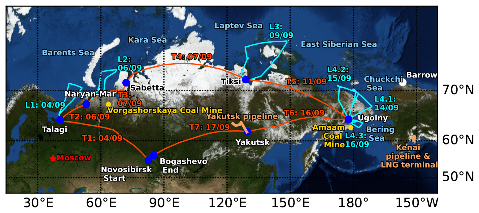
Figure 1September 2020 campaign flight plan. The 13 flights are indicated as either “loop” (prefix L, cyan line) or “transit” (prefix T, orange line). Oil and gas (O&G) infrastructures and coal mines are shown in light orange and yellow respectively (Global Coal Mine Tracker, 2022; Global Fossil Infrastructure Tracker, 2022), the data are under the Creative Commons License, https://globalenergymonitor.org/creative-commons-public-license/ (last access: 19 September 2021). Map background: “Blue Marble Next Generation”, September 2004 (Stöckli et al., 2005).
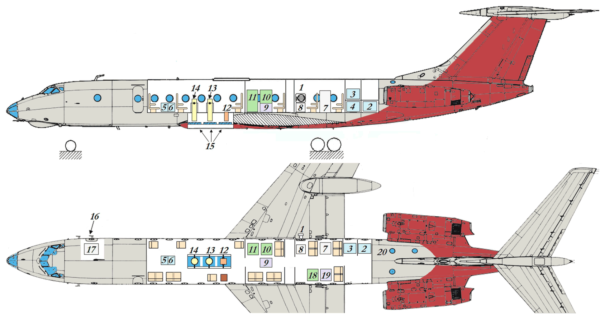
Figure 2Arrangement of the instrument suite on board the OPTIK TU-134 aircraft laboratory: 1 – ambient air inlets and relative humidity–temperature probe; 2 – aircraft electrical power distribution unit (28 V DC); 3, 4, 5, 6 – inverters (28 V DC/220 V AC) and uninterruptible power supplies (UPSs; Delta RT-2K); 7 – aerosol instrument rack (aethalometer, MDA-02; photoelectric aerosol nephelometer, FAN-M); 8 – aerosol instrument rack (diffusional particle sizer, DPS; optical particle counter, Grimm 1.109; filter; and bioaerosol sampling suite); 9 – navigation system (CompaNav-5.2 IAO); 10 – gas analysis rack (CO2–CH4–H2O; Picarro G2301-m); 11 – gas analysis rack (O3, TEI model 49C; CO, TEI model 48C); 12 – spectroradiometer (Spectral Evolution PSR-1100F); 13, 14 – aerosol lidars; 15 – camera hatches; 16 – ambient air inlet; 17 – sampling unit for organic aerosol analysis; 18 – gas analysis rack (NOx; Thermo Scientific model 42i-TL); 19 – main data acquisition system (NI PXI-1042); 20 – GLONASS/GPS antennas. Figure and caption by Belan et al. (2022).
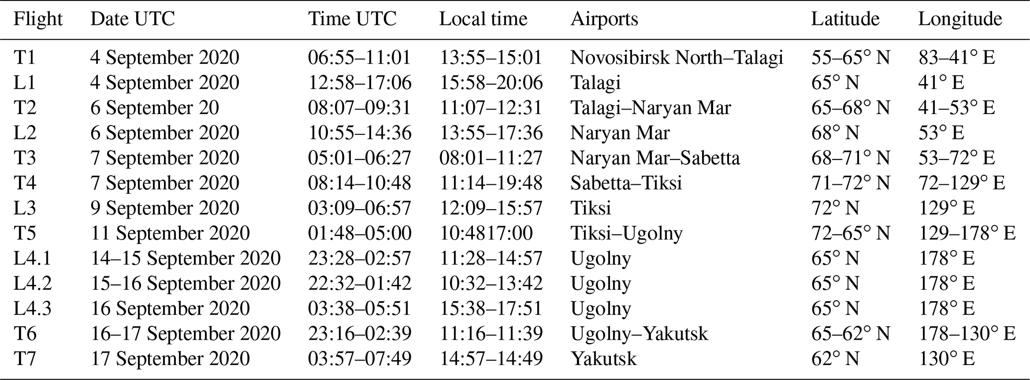
Figure 3 shows the geopotential height at 500 hPa as provided in the dataset ERA5 from the European Centre for Medium-Range Weather Forecasts; (ECMWF; Hersbach et al., 2018) on 6 and 15 September. At the beginning of the campaign (Fig. 3a), there was a low-pressure system over central Siberia (60∘ N, 80∘ E) and a high-pressure ridge coming from western Europe and going in a northeasterly direction to the Barents and Kara seas. The period was characterized by an “Omega” whirling around troughs over eastern Europe and eastern Asia that can be seen distinctly at the end of the campaign (Fig. 3b). The combination of these two events lifted an air mass most likely affected by western European emissions into the free troposphere over Siberia during the campaign. This may have influenced greenhouse gas concentrations as measured during the campaign. Over eastern Siberia (55∘ N, 180∘ E), there was a low-pressure system and winds blown from western Alaska to the Bering Strait (Fig. 3b).
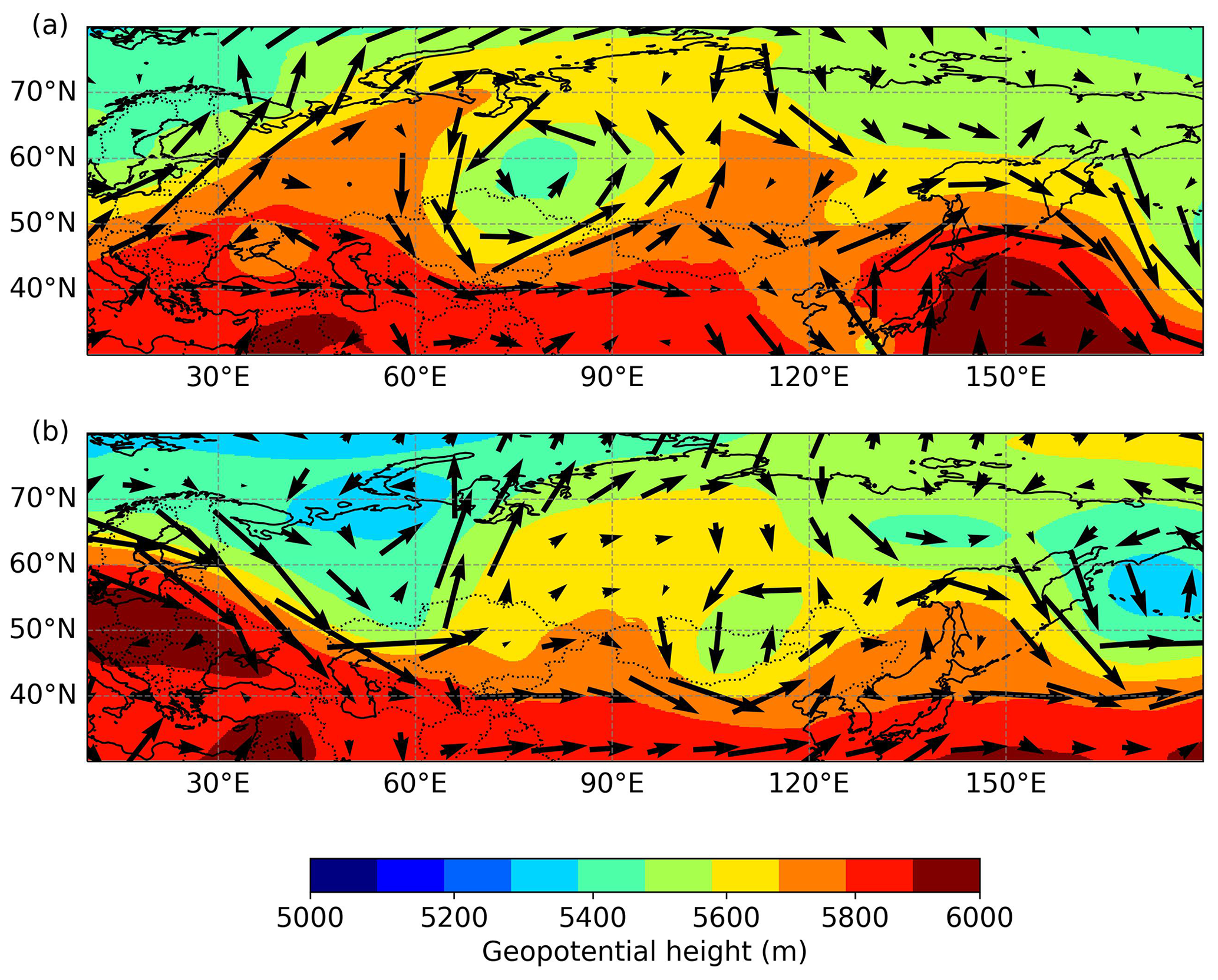
Figure 3(a) Geopotential height and wind (speed and direction) at 500 hPa from ECMWF reanalyses for 6 September at 13:00 UTC. (b) Same as (a) for 15 September at 01:00 UTC.
A series of 47 vertical profiles were collected, each lasting between 20 and 30 min. Loop flights were composed of three ascending and descending profiles. Transit flights had only vertical profiles during take-off and landing and took place at high altitude (about 10 km) in between. The plane stayed at horizontal plateaus when top altitudes were reached between 9000 and 11 000 m, as well as close to the ground at about 200 m and some on descents at 5000 and at 500 m. About 80 % of the data were acquired above 2000 m, which is generally above the planetary boundary layer (BL) at these latitudes and this time of the year. A total of 60 % of the measurements were taken north of the Arctic Circle (>66∘ N).
2.2 Instrumentation of the campaign
For in situ analysis air is sampled from inlets. The length of the tubes between the inlets and instruments was 4.8 m. Mixing ratios of CO2 and CH4 were measured by a Picarro G2301-m greenhouse gas (GHG) analyzer using cavity ring-down spectroscopy. It is a modification of the G2301 model specially conceived for aircraft measurements, which is designed to minimize effects induced by aircraft vibration and roll and is suitable for rapidly changing altitude (up to 1000 m min−1). It has an acquisition rate of 1 Hz and a precision of <0.20 ppm for CO2 and <1.5 ppb for CH4. Water vapor mole fraction is also quantified to include internal water dilution correction and thereby express dry air mixing ratios of carbon dioxide and methane. Three calibration gases are transported in high-pressure cylinders with respective CO2 mixing ratios of 370.91 ± 0.005, 390.33 ± 0.009, and 430.30 ± 0.006 ppm and CH4 mixing ratios of 1814.35 ± 0.150, 1960.99 ± 0.094, and 2205.01 ± 0.106 ppb. Their values were determined before the campaign at Laboratoire des Sciences du Climat et de l'Environnement (LSCE) according to World Meteorological Organization (WMO) standards (Paris et al., 2008). The drift is then corrected according to the difference between the measurements and the calibrated value of the reference gas. The whole campaign has been sampled at an interval of 1 s without data gaps, except for the transit T1 (the first of the series), during which the instrument software froze for the first half of the flight and was restarted after. The calibrated measurements can be compared to values of stations considered to be reference sites for species measured during September 2020:
-
Mauna Loa, Hawaii (19.54∘ N, 155.58∘ W; 3397 m a.s.l.) (Oltmans and Levy, 1994; Dlugokencky et al., 2021a, b) for CO2, CH4, and O3;
-
Mace Head marine sector, Ireland (53.20∘ N, 09.54∘ W; 25 m a.s.l.) (Hazan et al., 2016) for CO2, CH4 and CO (marine sector means that a selection on data based on standard deviation, wind speed, and wind direction has been made to only keep air masses from westerly sectors; Biraud et al., 2000);
-
Barrow, Alaska (71.32∘ N, 156∘ W; 11 m a.s.l.; see Fig. 1) for CO2 and O3.
Ozone was measured by a commercial fast-response ozone analyzer (Thermo Environmental Instruments model 49C USA), with modifications for internal calibration and aircraft operation safety. It is based on UV absorption in two parallel cells and has a precision of 2 ppb for an integration time of 4 s. In practice, values have been acquired with periods that vary between 4 and 10 s. Air is pressurized prior to the detection by a Teflon KNF Neuberger pump model N735 also used for CO. Before the campaign, the instrument was calibrated against a NIST (National Institute of Standards and Technology)-related reference calibrator model 49PS, and verification of the O3 analyzer was made before and after the campaign. The length of the Teflon tubes between the inlet and O3 and CO analyzers was 2 m.
Carbon monoxide is acquired by an instrument based on a commercial infrared absorption correlation gas analyzer (Thermo Electron model 48C, USA). It has been improved with the addition of periodical in-flight accurate zero measurements, a new IR detector, pressure increase and regulation in the absorption cell, increased flow rate to 4 L min−1, a water vapor trap, and an ozone filter. The response time of the instrument is 30 s, and it has a precision of 5 ppb, with a lower detection limit at 10 ppb (YAK-Aerosib Measurements, 2021). For this campaign, the CO data were not post-processed due to technical problems and were therefore of lower quality than in previous studies. We applied a median filter with a kernel size of 75 samples. When computing the statistics for each flight, CO standard deviations ranged between 10 and 35 ppb for mean mixing ratios between 73 and 103 ppb. In the present study, CO measurements are discussed as tracers for analysis of the other gases. To be compared with simulations (see Sect. 3.4), the measured mixing ratios were 1 min averages with the background removed. The background is defined for each flight as follows: (1) only CH4 values in air that had a corresponding O3 mixing ratio <70 ppb were kept to remove influence from air of fresh stratospheric origin, (2) then the 5th percentile of the remaining data was taken as the background value. Background mixing ratios were calculated flight by flight.
2.3 Back trajectories with the Lagrangian model FLEXPART
We used the Lagrangian particle transport and dispersion model FLEXPART (Stohl et al., 1998; Stohl and Thomson, 1999; Stohl et al., 2005; Pisso et al., 2019) for long-range transport analysis and for determining the origin of the polluted air masses measured during the campaign. We adopted the backward (“receptor-oriented”) approach of the model, which is suitable when the number of sources is superior to the number of receptors and designed to quantify the remote contributions in a single plume (Seibert and Frank, 2004). In our configuration FLEXPART computed the position of 2000 particles backwards in time, following the atmospheric conditions with a stochastic contribution representing the diffusion (including small-scale turbulence not included in averaged meteorological fields) (Fleming et al., 2012). These implementations allowed a more realistic representation of transport in the planetary boundary layer. The lifespan of the virtual particles was set to 10 d as the transport precision decreases after 10 d due to accumulated transport errors and insufficient number of particles to represent it (Stohl et al., 1995). The meteorological inputs were ERA5 datasets from ECMWF with a spatial resolution of 1∘ and a temporal resolution of 3 h covering the Northern Hemisphere, limiting the resolution of the output grid to 0.5∘ × 0.5∘. A simulation was performed for each flight, beginning 10 d before the first acquisition and ending with the last acquisition. Receptor (i.e., aircraft) positions every 1 s during the campaign are aggregated in four-dimensional boxes (0.1∘ × 0.1∘ × 100 m × 60 s). The potential emission sensitivity (PES) calculated by the model for each receptor position is defined as the residence time of the backward particles in a grid cell below a threshold altitude (here 500 and 2000 m). We convolved this output with CH4 flux inventories to get maps of potential source contributions that are integrated over the Northern Hemisphere to finally get the simulated mixing ratios of each source every minute.
2.4 Methane flux inventories
For our simulations, five categories of CH4 sources were considered:
-
Emissions of CH4 by anthropogenic activities were characterized with EDGAR v6.0 (Emission Database for Global Atmospheric Research from the PBL Netherlands Environmental Assessment Agency) with a grid resolution of 0.1∘ × 0.1∘ (Crippa et al., 2019). EDGAR inventories are published as yearly or monthly files. We chose to use the month of September 2018 (the last available) to benefit from the seasonality of the emissions. We aggregated the 21 EDGAR sectors into three categories – agriculture, exploitation and use of fossil fuels, and waste management (see grouping definition in Table B1).
-
Biomass burning and wildfire emissions were represented using GFED4.1s (Global Fire Emissions Database) based on van der Werf et al. (2017) at a resolution of 0.25∘ × 0.25∘ for the monthly mean of September 2020.
-
Wetland fluxes were based on the process-based model ORCHIDEE as described in Ringeval et al. (2012) at a horizontal resolution of 0.5∘ × 0.5∘ for September 2017 only for the Northern Hemisphere provided to the Global Carbon Project 2019 (Melton et al., 2013; Wania et al., 2013; Zhang et al., 2021).
-
The representation of freshwater CH4 fluxes, based on the work of Thonat et al. (2017), combined two inventories – the lake biogeochemical model (bLake4Me) (Tan et al., 2015) for sources above 60∘ N and Global Lakes and Wetlands Database (GLWD3) distribution for the rest of the Northern Hemisphere (Lehner and Döll, 2004), with a resolution of 0.25∘ × 0.25∘ based on data from 1971 to 2013.
-
The ocean fluxes were based on the work of Weber et al. (2019), a synthesis of measurements made between 1980 and 2016 with an output grid at 0.25∘ × 0.25∘ resolution from the MarinE MethanE and NiTrous Oxide (MEMENTO) database (Kock and Bange, 2015). The total marine fluxes are provided as diffusive fluxes from sediments to the surface and ebullition of bubbles released from bottom sediments that reached the atmosphere. We combined the two fluxes in one emission map.
When it was possible, we preferred using inventories averaged for September instead of inventories averaged for several months to put an emphasis on the seasonality of emissions. All inventories were re-gridded to 0.5∘ × 0.5∘ in order to be aligned with the grid of the FLEXPART footprints. Figure B1 illustrates the fluxes indexed by inventories from fossil fuel emissions, agriculture, wetlands, freshwater, and oceans in the Northern Hemisphere.
3.1 Distribution of CH4 and CO2 during the campaign
Hereafter we refer to “low altitude” and “high altitude” for data that are respectively acquired below and above an arbitrary altitude threshold of 2000 m. The majority (80 %) of the data have been measured at high altitude. Low-altitude measurements are analyzed separately to highlight sensitivity to local or regional sources. Reported uncertainties are 1σ uncertainties.
3.1.1 CH4 mixing ratios
The average CH4 mixing ratio of the campaign is 1946 ± 45 ppb. This is higher than the monthly mean mixing ratio measured at Mauna Loa of 1887 ppb used as a hemispheric reference. Figure 4a shows that the median value of each flight (except for T6) is above the Mauna Loa mean value. At low altitude, the average mixing ratio is higher, with a value of 2011 ± 33 ppb, and so it exceeds mixing ratios observed at Mauna Loa, Mace Head marine sector (1956 ppb), and Barrow (1991 ppb). This suggests the possible influence of significant regional methane sources. Many flights present a high CH4 variability. Flights in the western Siberian Arctic have the highest 3rd quartile of the campaign (L1, L2, and T2), then followed by the flights in the eastern Arctic (L3, L4.2, and L4.3). Large mixing ratios are expected to be encountered in the boundary layer, linked to regional sources; these are discussed in the Sect. 3.2 by using vertical profiles. Flights T1 and T6 registered the lowest CH4 mixing ratios of the campaign (respectively 1812 and 1777 ppb, with an aircraft altitude above 10 000 m), coming from stratospheric air masses, which results in strong gradients for these two flights.
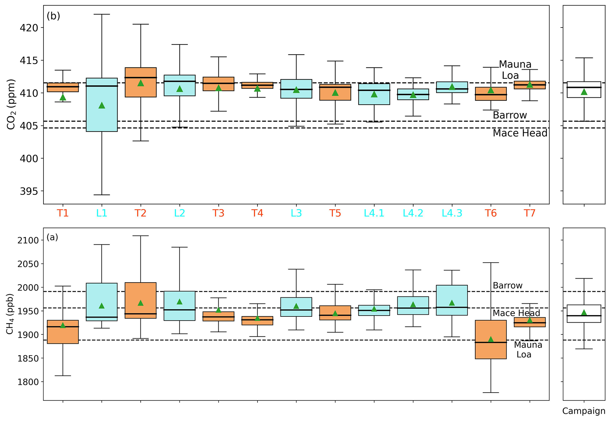
Figure 4(a) CH4 mixing ratio variability by flight. Statistics for the entire campaign are shown in the right panel. The boxplot shows the interquartile range (25 %–75 %) and the median value. The whiskers extend to the lowest and highest values, ignoring outliers beyond 1.5 times the interquartile range. Flight means are shown as green triangles. Dashed lines show respectively the mean monthly mixing ratios at Mauna Loa and Mace Head marine sector during September 2020. (b) Same as (a) for CO2.
Generally, loop flights exhibit a higher first quartile than transit flights for low-altitude values. These specific flights have indeed longer low-altitude legs and overall more frequent passages at low altitude (three ascents and descents for loops versus one ascent and one descent only for transits).
3.1.2 CO2 mixing ratios
The average CO2 mixing ratio of the campaign is 410.17 ± 3.29 ppm, slightly below the seasonal average at Mauna Loa (411.52 ppm) but higher than Mace Head marine sector and Barrow values (respectively 404.62 and 405.67 ppm). Figure 4b presents the mixing ratio statistics for each flight and the whole campaign. Almost all median values are below the Mauna Loa reference, suggesting that air masses observed during the campaign may have intersected with regional CO2 sinks. Candidate areas potentially explaining the sink include all terrestrial biomes in Russia (Bartalev et al., 2003; Belikov et al., 2019; Petäjä et al., 2021). Flight T1 flying over the western Siberian taiga exhibits median values at low and high altitude respectively of 397.73 and 410.92 ppm (with a standard deviation of 4.30 ppm), highlighting the influence of these sinks. This biospheric uptake by Siberian boreal ecosystems (>50∘ N) has already been observed during previous YAK-Aerosib campaigns realized in late August or early September. Vertical profiles for western flights at this time of the year present low CO2 concentrations close to the surface jointly with a positive strong gradient when the altitude is increasing (Paris et al., 2008, 2010a). Paris et al. (2010b) demonstrated based on the relation between measured CO2 concentration and air masses' residence time in the lowest 300 m that for the September campaign, the longer the air masses resided over local areas (boreal and sub-arctic Siberia, >50∘ N), the stronger the CO2 uptake by Siberian ecosystems.
Two flights (L1 and T2) exhibit a large variability compared to the rest. For both flights, there are considerable gradients in CO2 mixing ratios (+15 and +10 ppm for respectively L1 and T2) between high and low altitudes, suggesting the presence of effective sinks (forests and oceans in this case) at low altitude and the presence of “polluted” air masses at high altitude from long-range transport.
The highest mixing ratio measured during the campaign (451.85 ppm) was registered at the end of flight T6, while the aircraft was landing at the airport of Yakutsk. This is most likely driven by local pollution. At the time of landing the airport was fogged in (the aircraft was landed with difficulty due to the absence of enough fuel for flying to an alternate airfield).
3.1.3 Comparing CO2 and CH4 variabilities
When comparing CO2 and CH4 profiles, two different types of flights appear: (1) both CO2 and CH4 present high variability, such as on flights T2, L1, L2, or L3, illustrating active regional sources for both species and a strong uptake for CO2; (2) CH4 presents high variability (with relatively low values), while CO2 is steady, such as on flights T1 and T6. For CH4, it illustrates the influences of strong regional emissions for the highest values and of influx of stratospheric air for the lowest values. The CO2 measured is subject to an attenuated vertical propagation of seasonal surface fluxes as demonstrated in Gerbig et al. (2003), leading to this relatively smaller variability during mostly high-altitude transit flights. To put these limited observations of the greenhouse gas variability into perspective, the following section discusses vertical distribution of mixing ratios.
3.2 Average vertical distribution of the gases
All data were binned every 1000 m in a range of ±500 m to get vertical profiles in Fig. 5. Data were also stratified according to their longitude, separating regions west and east of the 130∘ E meridian. As reported in Sect. 3.1, western flights exhibit a large vertical gradient in mean gas mixing ratios (high- minus low-altitude means ranging between −64 and −109 ppb, +9.10 and +14.80 ppm, and −14 and −29 ppb respectively for CH4, CO2, and O3) compared to eastern flights.
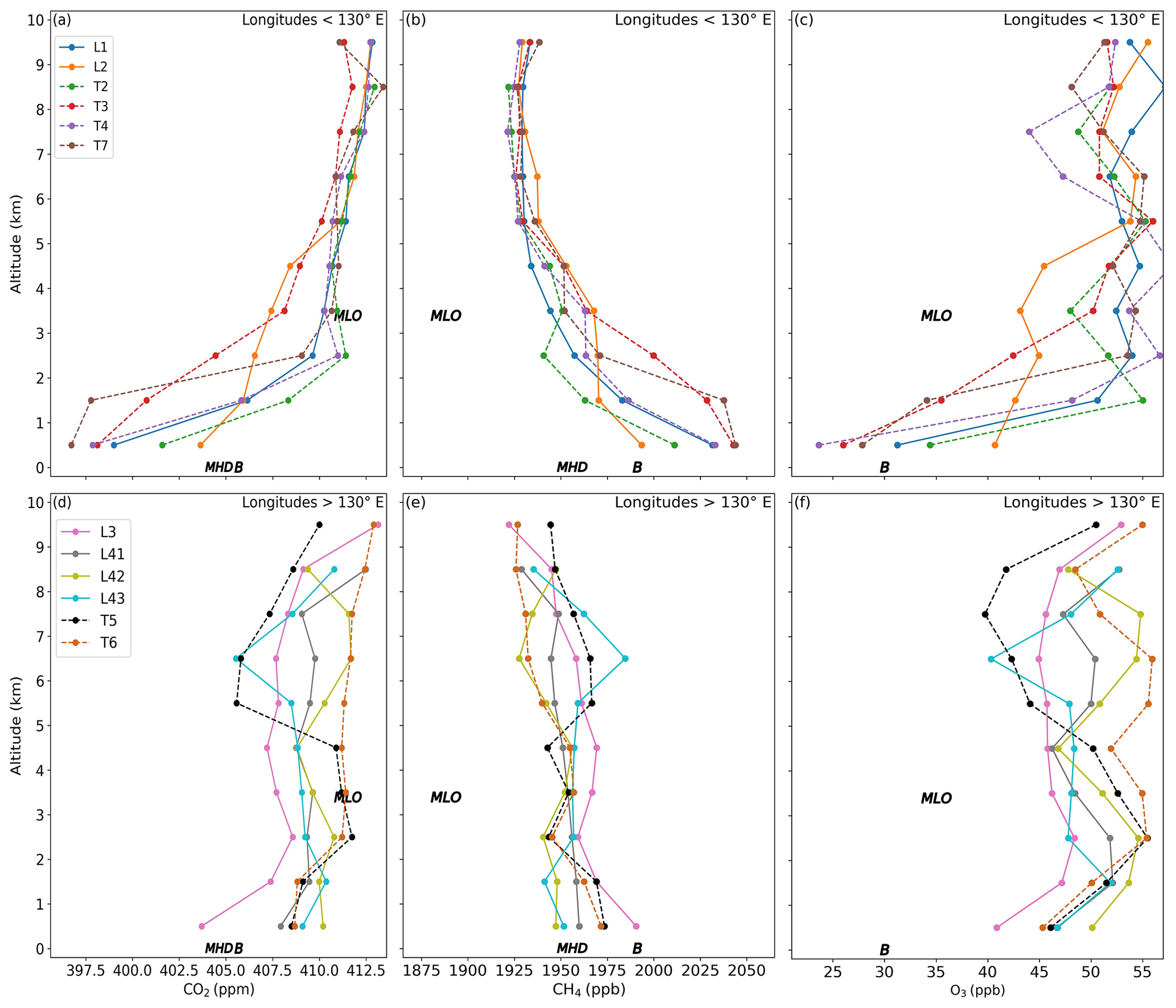
Figure 5Flight mean vertical mixing ratio profiles for CO2 (a, d), CH4 (b, e), and O3 (c, f). Top row shows flights west of 130∘ E, while the bottom row shows flights east of 130∘ E. Flight T1 is not shown due to missing data. Monthly mean values at Mauna Loa (MLO), Mace Head marine sector (MHD), and Barrow (B) in September 2020 are shown in each panel.
For CH4 at low altitude, western flights (Fig. 5b) present higher mixing ratios than eastern flights (Fig. 5e), with the biggest values in T3 and T7, closely followed by L1 and T4. Another feature of western flights is the difference in gradient between low and high altitudes: all western flights except L2 have a much steeper gradient between 0 and 3000 m (ranging from −74 ppb for L1 to −42 ppb for T3 with increasing altitude) than between 3000 and 10 000 m (ranging from +11 ppb for L1 to +38 ppb for L2 with increasing altitude). Combining this information with the observation of the biggest CH4 mixing ratio close to the ground indicates a strong local source, the Ural wetlands, as reported in Belikov et al. (2019). At high altitude, no conclusion on the origin of the influences can be made at this moment. This is investigated in Sect. 3.4.1 using the simulated CH4 enhancements and the footprints. In contrast, low-altitude values for eastern flights (Fig. 5e) are encompassed in a range between 1947 and 1990 ppb. These mixing ratios still represent an enhancement of +60 ppb to +100 ppb compared to the hemispheric reference (Mauna Loa monthly mean) of 1888 ppb. The references of Mace Head marine sector and Barrow respectively at 1956 and 1991 ppb are in the same range as the easternmost flights' low-altitude values but below western flights' low-altitude values. The simulated enhancements presented in Sect. 3.4.1 are also necessary to identify the sources at the origin of the CH4 measured here. For flights T5 and L4.3, a layer of elevated CH4 mixing ratios is crossed in the mid-troposphere between approximately 6 and 8 km altitude (Fig. 5e). On flight L4.3, for example, the vertical CH4 gradient represents an excess of ∼20 ppb between 6500 and 8500 m compared to the underlying layer (between 4500 and 6500 m). This increase in CH4 at top altitudes for flight L4.3 correlates with a decrease in O3 mixing ratio of −10 ppb between 7500 and 8500 m and a decrease in CO2. The possible origin of this high-altitude O3 depletion is investigated in Sect. 3.3.1 using individual vertical profiles that exhibit the same distribution for other flights such as L3 (also T4 or L2, not shown in the study).
O3 vertical profiles generally increase with altitude, especially on the western flights, and follow a trend opposite to that of CH4 mixing ratios. Eastern flights present an enhancement of +10 to +20 ppb as compared to respective Mauna Loa and Barrow mixing ratios of 35 and 30 ppb for the same altitude range, while western mixing ratios agree with the value from Barrow but are above the one from Mauna Loa. O3 and CH4 measurements are above the corresponding reference values and therefore reflect regional variability in transport that need deeper investigation.
For CO2, our measurements are comparable to the Mauna Loa monthly mean (411.52 ppm) in the free-tropospheric altitude range of the site (2000–3000 m). Mean CO2 measured during the western flights in the lowest 1000 m (397–403 ppm) is consistently lower than Mace Head marine sector and Barrow monthly means (respectively 404.62 and 405.67 ppm). As for CH4, all western CO2 vertical profiles (except for L2) have a steeper gradient between 0 and 3000 m (ranging from 6.3 for T3 to 13.1 ppm for T4 with increasing altitude) than between 3000 and 10 000 m (ranging from 0.4 for T7 to 3.2 ppm for T3 with increasing altitude), conjointly supporting the inference made in Sect. 3.1.2 on the strong uptake by Siberian ecosystems. In contrast, eastern flights except L3 present mean CO2 mixing ratios below 1000 m higher than Mace Head marine sector and Barrow means. The four highest mean CO2 mixing ratios close to the ground are collected during eastern profiles (Fig. 5d). These are the three loops of Bering Strait and the transit T6 landing at Yakutsk. For flight T6, half of the low-altitude values were taken in the vicinity of the city of Yakutsk and could be subject to local pollution. Concerning the city of Yakutsk, CH4 also presents high mixing ratios at low altitudes with values of 1972 and 2045 ppb for respective flights T6 and T7. The highest average mixing ratios at low altitudes for CO are also measured during flights T6 and T7, with similar values of 103 and 107 ppb respectively. The loops L4.1, L4.2, and L4.3 in remote marine environments are investigated in Sect. 3.2.2. Flights L4.3 and T5 present a lower-CO2 layer at higher altitude (respectively 6500 and 5500 m) already noted previously.
These observations show that the atmosphere over Siberia is affected by a complex pattern of influences from local emissions and long-range transport of polluted air masses. It highlights the importance of untangling the different influences on atmospheric composition (Petäjä et al., 2021) discussed in the next section.
3.3 Individual vertical profiles and regional atmospheric transport
3.3.1 Northwestern Russia
Figure 6 displays four selected profiles (either ascent or descent) that are representative of vertical distribution of trace gas mixing ratios encountered during the campaign. Figure 6a is a profile of flight L1 characterized by taiga and wetland environments. The flight L1 is highlighted in Sect. 3.1.1. for having the largest CO2 interquartile range of the whole campaign. Figure 6b is a profile of flight L3 close to the ESAS. Figure 6c shows a profile of flight T7 crossing the city of Yakutsk in regions covered by forests of coniferous trees and agricultural lands, and Fig. 6d represents a profile of flight L4.1 located near the Bering Strait in biomes such as Arctic deserts, tundra, and forest tundra.
The vertical profile shown in Fig. 6a presents a large CO2 depletion of 14 ppm in the lowest 2000 m depth layer, highlighting the strong drawdown of CO2 in BL air. Higher-altitude air corresponds to free-tropospheric air masses that mostly resided over western European countries and the United States to finally arrive in Russia from high altitudes (see footprint in Fig. 7a). These regions are important CO2 and CH4 emitters through fossil fuel exploitation and combustion, agriculture, and waste management as documented in the EDGAR inventories (Crippa et al., 2019). This shows that the tropospheric air over the area of flight L1 is dominated by the outflow of European BL air interplaying with CO2 uptake in the BL. Both CH4 and O3 profiles present an inversion corresponding to a “chemical” BL around 1000 m (with gradients respectively −90 and +25 ppb). Below 3000 m, CH4 is anti-correlated with O3, while the two gases present common features above this altitude, with thin positively correlated layers at 4000 and 5000 m.
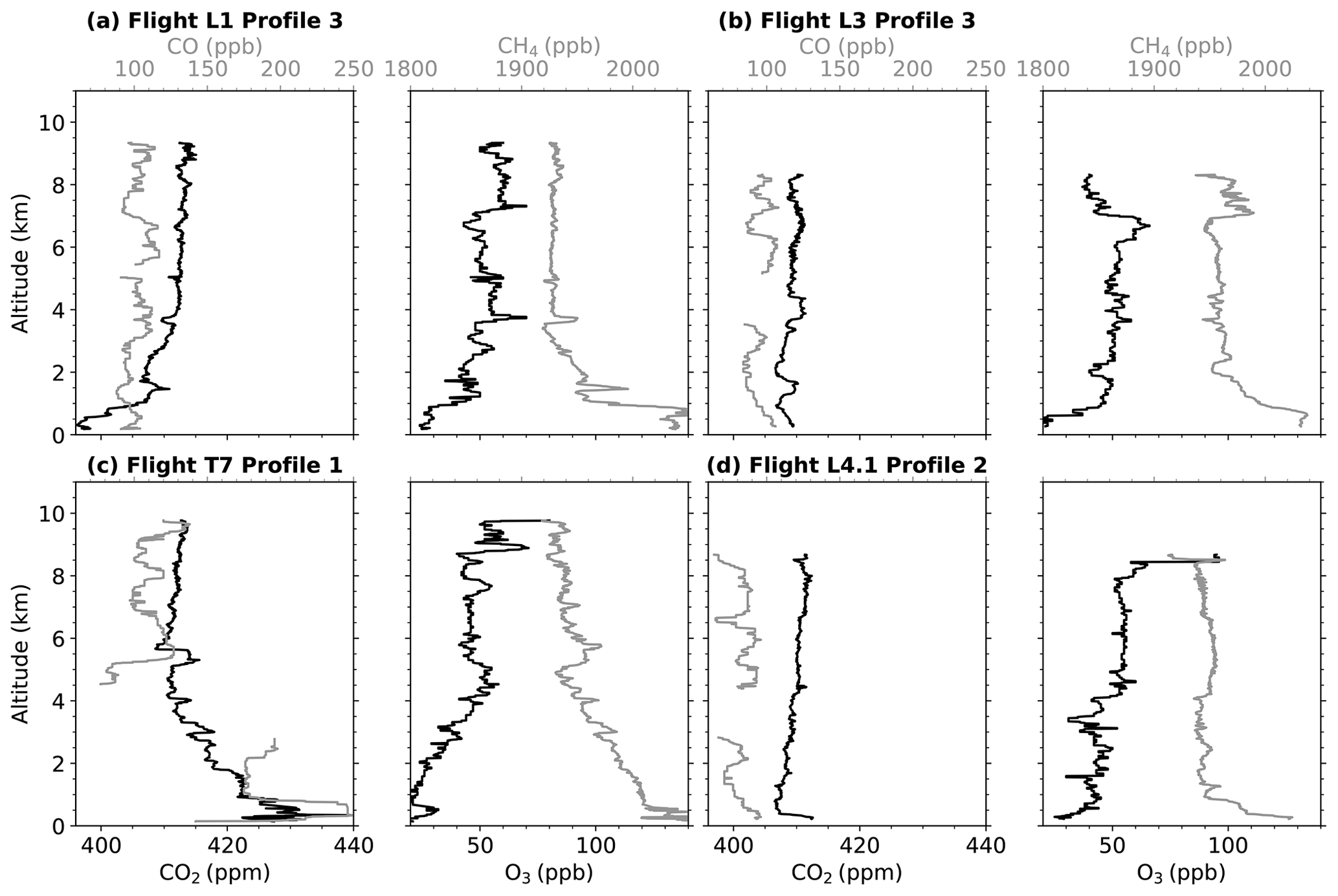
Figure 6Four selected vertical profiles of the campaign. CO2 and CO are respectively in black and gray on each left plot. O3 and CH4 are respectively in black and gray on each right plot.
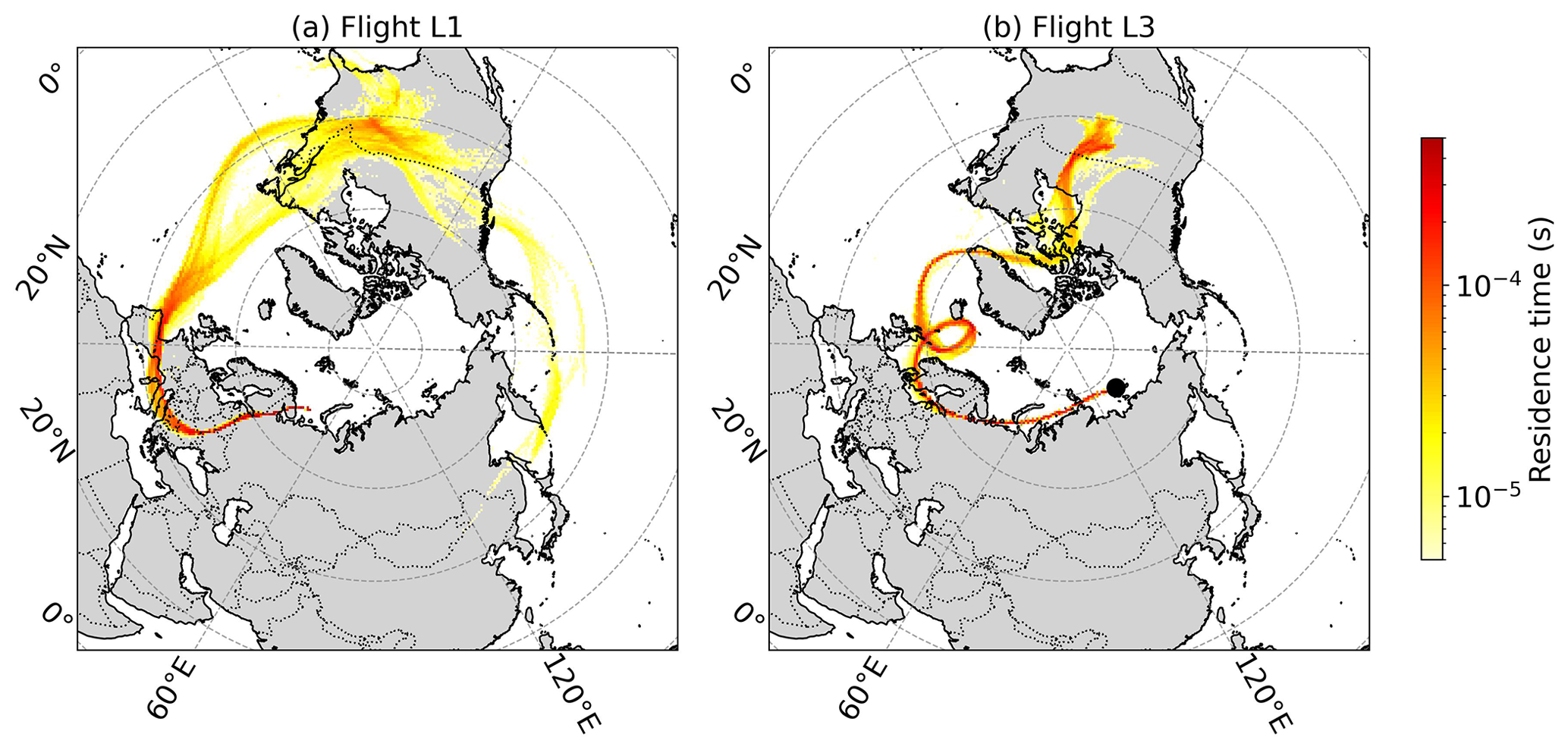
Figure 7Total column footprints for simulated retro-transport of particles released at 14:53 UTC at an altitude of 9324 m during flight L1 (a) and at 05:01 UTC at an altitude of 5256 m during flight L3 (b). The black dot represents the receptor position.
Figure 6b shows the second ascent of L3, in the north of Siberia. Here, CO2 mixing ratio shows less variability than flight L1 profile 3. A slight decrease of −3 ppm of CO2 and −20 ppb of CO with altitude can be observed under 1000 m, possibly indicating the influence of emissions by local combustion, although this ascent does not start at an airport. We can also observe a stratification in the CO2 and CO profiles with mixing ratio changes in stacked layers whose thickness varies between 500 and 1500 m. This stratification has already been observed in previous campaigns (Paris et al., 2008) and is due to slow stirring in the troposphere under reduced vertical mixing. This profile is also characterized by significant sources of CH4 in the BL as suggested by the strong enhancement of 100 ppb close to the ground (Fig. 6b). Among potential sources is methane hydrate degradation from the East Siberian Arctic Shelf (Berchet et al., 2016; Thornton et al., 2016; Berchet et al., 2020). The influence of potential sources is discussed in Sect. 3.4. In the same profile, O3 is anti-correlated with CH4 above 3000 m, except at the top altitude around 8500 m, where O3 mixing ratios unexpectedly decrease closer to the stratosphere. This O3 depletion mentioned in Sect. 3.2. (−24 ppb compared to immediately lower layers) occurs in the air mass whose history is shown in Fig. 7b. The same backward transport simulation with a threshold altitude of 500 m (Appendix Fig. C1) shows an air mass coming from the BL in North America, then crossing the Atlantic Ocean and northern Europe (only visible on the total column footprint). This layer with poor ozone mixing ratio is likely to be an uplift of BL air with the origin of the depletion potentially coming from another location further upstream. The O3 mixing ratio at the top altitude varies from 37 to 40 ppb, which is comparable to local mixing ratio at 2000 m (40 to 42 ppb) of the same flight or flight L1 (41 to 42 ppb just under 2000 m), corresponding to regional BL air.
3.3.2 Yakutsk urban area
Another singular event previously mentioned was a possible pollution enhancement in the area of Yakutsk. The corresponding vertical profile in Fig. 6c shows high CO2, CH4, and CO mixing ratios (respectively 439.60 ppm, 2070 ppb, and 251 ppb) as the aircraft took off from Yakutsk. At low altitude, both CO and CH4 present high correlation with CO2 (respectively R2=0.92 and R2=0.84) as shown in Fig. 8a and b, while there is no correlation at higher altitude. This suggests combustion emissions possibly related to fossil fuel exploitation and/or use. This region is indeed characterized by the presence of operating O&G infrastructures and coal mines (Fig. 1). We can also observe the lowest O3 mixing ratio of the campaign at 2 ppb at the ground level of Yakutsk (value too low to be seen in the figure). Having this O3 near-ground minima over landing air strips in polluted city plumes of Yakutsk suggests a titration of O3 by NO.
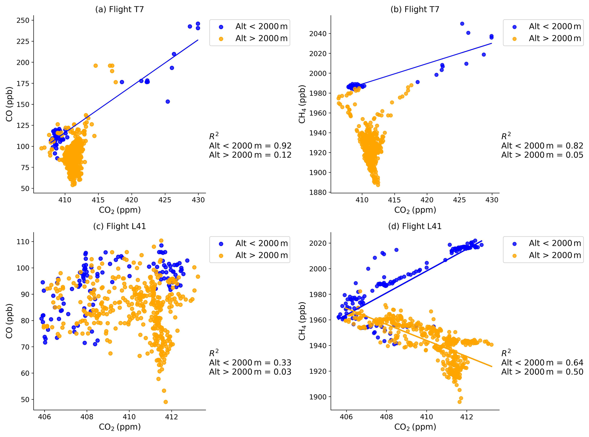
Figure 8Scatterplots of CO2 vs. CO (a) and CO2 vs. CH4 (b) for flight T7. Same for flight L4.1 in (c) and (d). Blue dots and respective regression lines are for data acquired under 2000 m. Orange dots and respective regression lines are for data acquired above 2000 m. Correlation coefficients R2 are displayed for each set.
3.3.3 CO2 enhancement at low altitude in the Far East
Although the average CO2 profiles of flights L4.1, L4.2, and L4.3 show little variability over the Bering Strait, we find significant CO2 enhancements at very low altitude (<500 m; Sect. 3.2). Here we focus our analysis on the loop L4.1 as the three flights have similar features. In the vertical profile of the first descent (second profile), remote from any airport, a high CO2 mixing ratio of 412.5 ppm has been observed close to the surface (200 m), against 407 ppm at 500 m altitude (Fig. 6d). The CH4 mixing ratio also decreases from 2025 to 1980 ppb between 200 and 500 m altitude. On the other hand, CO presents only a small, opposite gradient of about −10 ppb across the same altitude range. Above 500 m, the CO2 profile exhibits a more typical shape of marginally increasing vertical gradient.
Figure 8c shows a scatterplot of CO against CO2 for the whole flight L4.1 (including all six profiles). The correlation coefficient under 2000 m is significant but slightly lower (R2=0.33, ) than correlation coefficients between CO2 and CH4 shown in Fig. 8d (R2=0.64, ), suggesting that the CO2 enhancement may be driven by a mixture of emissions including local combustion processes. The regression slope below 2000 m is 8.5 ppb of CH4 per part per million of CO2. Non-combustion sources emitting both CO2 and CH4 leading to such a signature could include one or several fossil fuel exploitation areas co-emitting the two species. According to the Global Fossil Infrastructure Tracker map from Global Monitor Energy, no operating O&G pipeline or terminal is reported in the eastern Siberian region, and the closest one is the Kenai Alaska liquid natural gas terminal (Fig. 1). Still according to Global Energy Monitor, only Amaam North Coal Mine is active in the eastern Siberian region (Fig. 1), but there are other coal mine activities reported in the Russian Far East (Petäjä et al., 2021). Section 3.4.1 below shows that influences on this part of the flight L4.1 are mostly of natural origin and linked to the potential emission sensitivity of Alaskan emissions. Multiple regional and diffuse sources may be at play in explaining the enhancement observed. Another possibility is an emission from marine CH4 sources. The absence of sea ice at the time of the campaign in the involved area (Fig. A1) (Fetterer et al., 2017) enables air–sea exchange, notably for CH4.
The anti-correlation between CO2 and CH4 above 2000 m (Fig. 8d) could be a residual from active sources for CH4 and active sinks for CO2 during the summer. While the air in this region has been relatively well mixed as shown by the flat vertical profiles of CO2 and CH4 for flights L4.1, L4.2, and L4.3 (Fig. 5) and the reduced value ranges for CO2 and CH4 on the scatterplot of Fig. 8d (compared to the value ranges in Fig. 8b), mixing of air masses affected simultaneously by CO2 sinks and CH4 sources in the past might be incomplete, resulting in this residual anti-correlation. This is better investigated in Sect. 3.4.1 by using the simulated mixing ratios for flight L4.1.
3.4 Untangling the different methane sources with a Lagrangian model
3.4.1 Contributions to measured CH4 by source type and by location
This section aims at identifying the main emissions influencing the CH4 mixing ratios through case studies of selected flights. Figure 9 shows a scatterplot of measured and simulated CH4 enhancements for each flight. Enhancement here refers to the measured mixing ratio minus the background of the flight (background is defined in Sect. 2.3). Correlation coefficient R2 ranges between 0.28 (for flight T5) and 0.86 (for flight L1), with associated p values that are inferior to 10−10 for every flight. For most flights, the agreements between simulations and measurements are satisfactory and enable comparison of simulated source contributions to observed CH4 enhancements. However, the 1:1 dashed line highlights an underestimate of simulated mixing ratios discussed in this section and the next one. For the study, we select one flight in western Siberia, T2, which has a correlation coefficient R2=0.82, and one flight in eastern Siberia, L4.1, which has a correlation coefficient R2=0.67.
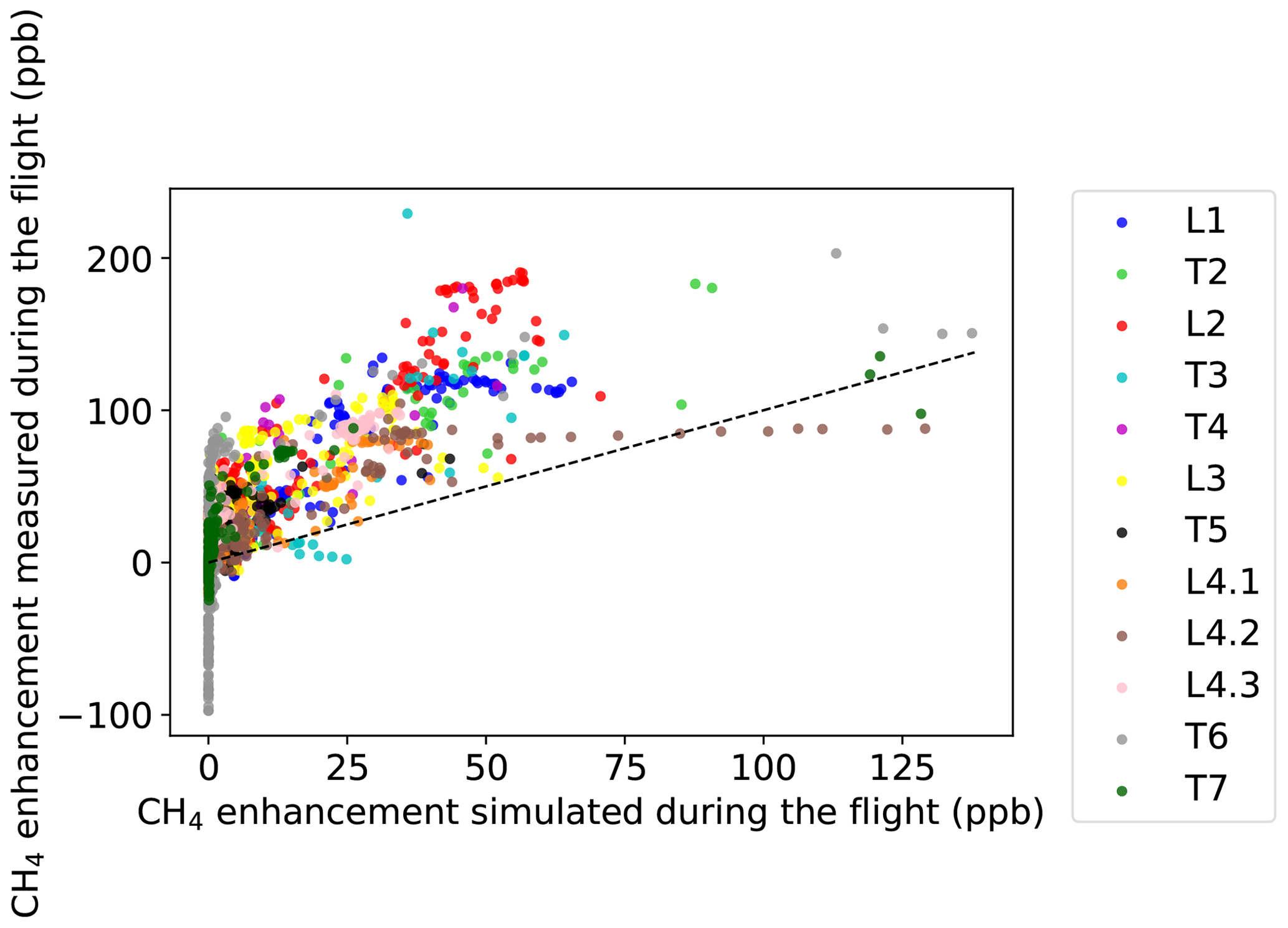
Figure 9Scatterplots of simulated CH4 enhancement vs. measured CH4 for each flight of the campaign except T1 with the 1:1 dashed black line. Data were aggregated into 1 min bins to produce this figure.
Figure 10 shows the simulated CH4 mixing ratios aggregating contributions from tagged sources during flight T2. The simulated signal at the receptor position is compared to measured CH4 enhancement. The CH4 enhancement variability is reasonably well reproduced by the model (Fig. 10a), but there is a consistent underestimation in total enhancement values. The possible reasons of this underestimate are discussed later in Sect. 3.4.2. However, the ability of the model to reproduce the peaks and trough of CH4 during the entire campaign allows some confidence in the comparative tagged tracer analysis intended here.
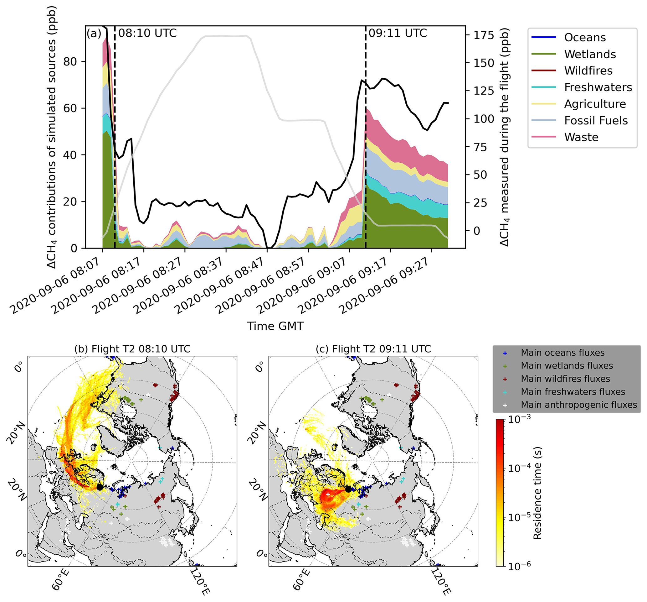
Figure 10(a) Simulated CH4 enhancement (colored stacked plot) and measured CH4 (black line) for flight T2. Note the different y axes. Altitude is shown in gray (bottom at 12 and top at 8963 m). The two vertical dotted lines indicate the measurements represented in the following footprints. (b) The 10 d potential emission sensitivity (PES) for particles released at 08:10 UTC. (c) Same as (b) at 09:11 UTC. The colored “+” symbols represent the fluxes with the biggest intensities derived from each inventory. The black dot represents the receptor position.
Figure 10b and c show PES for two selected positions representative of the flight. The footprint in Fig. 10b corresponds to the beginning of the ascent after leaving the airport (first dotted line at 08:10 UTC in panel a). At this position, an enhancement of 50 ppb was simulated. This enhancement is simulated to originate from a dominant anthropogenic contribution distributed between fossil fuel emissions, agriculture, and waste management for a total of 36 ppb (the next highest contribution being wetlands, with 10 ppb of contribution). The footprint in Fig. 10b shows that the air mass has mostly resided over western Russia; central Europe; the Atlantic; and, to a lesser extent, the USA (although this corresponds to an air mass age close to the limit of particle tracking of 10 d). This is consistent with the dominance of agricultural CH4 fluxes in anthropogenic fluxes in Europe and the USA (Appendix Fig. B1b), while agriculture is much less significant in the Russian emission inventories (Crippa et al., 2019). This documents long-range transport of free-tropospheric air masses with relatively high CH4 (comparable to values encountered in the BL) in western Siberia.
The footprint in Fig. 10c, close to the Arctic Ocean at lower altitude (second dotted line at 09:11 UTC in panel a), corresponds to mixed enhancements of 28 ppb by wetlands and 27 ppb by human activities. The PES is concentrated on western Russia, with a major sensitivity to anthropogenic flux at the core representing the city of Moscow (white-filled “plus” sign in Fig. 10c). The simulated enhancements are driven by the CH4 fluxes from fossil fuel exploitation and use (Appendix Fig. B1a) in western Russia and from wetland fluxes in western Siberia (Appendix Fig. B1c), especially in the Vasyugan swamp.
At the end of the flight, when getting closer to Naryan Mar, Fig. 10a depicts an enhancement of 7 ppb associated with freshwater sources that is represented by the constant light-blue area between 09:11 UTC and the last data at 09:31 UTC. A large number of lakes are present around Naryan Mar and its surroundings (Fig. D1), supporting the importance of freshwater contribution in the atmospheric CH4 burden. Also, it is likely that a part of the simulated enhancements due to wetlands may be associated with freshwater CH4 emissions because there may be some overlap in inventories regarding small lakes and wetland sources, especially in complex regions with the presence of many wetlands, lakes, or rivers like in Naryan Mar's outskirts.
Focusing now on eastern Siberia, Fig. 11 illustrates the simulated and measured CH4 enhancements and two PES footprints associated with two specific positions of the flight. Overall, measured and simulated enhancements are lower than for the western Siberian flight previously discussed. The first case (00:25 UTC during flight L4.1, first dotted line) is a very thin plume of elevated CH4 in the lower free troposphere. It has a simulated enhancement of 14 ppb dominated by contributions due to fossil fuel emissions (7 ppb), agriculture (4 ppb), and waste management (3 ppb). The PES footprint in Fig. 11b shows that the air masses have partially resided over northeastern China, very close to fossil fuel emission sources (see the white “+” sign in Fig. 11b) and where important CH4 fluxes from agriculture are present (Fig. B1). Several fossil fuel extraction infrastructures are located in this region (Global Fossil Infrastructure Tracker, 2022). A large part of the air masses have also resided over the East China Sea and Bering Strait, where there are CH4 fluxes due to offshore fossil fuel according to EDGAR inventories (Appendix Fig. B1), explaining the domination of fossil fuel emission contribution in the selected peak. Overall at altitudes above 2000 m, most contributions are missed by the model, showing that the air in the free troposphere has not been in contact with the surface for more than 10 d. This supports the anti-correlation observed in the Sect. 3.3.3 between CO2 and CH4 for flight 3.1, which is a residual of the active sources and sinks during the past summer.
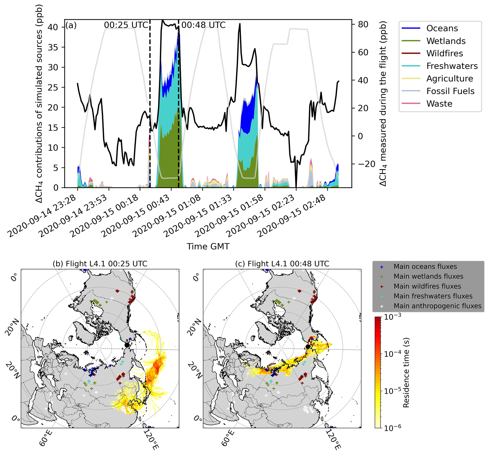
Figure 11(a) Simulated CH4 enhancement (colored stacked plot) and measured CH4 (black line) for flight L4.2. Note the different y axes. Altitude is shown in gray (bottom at 38 and top at 8707 m). The two vertical dotted lines indicate the measurements represented in the following footprints. (b) The 10 d potential emission sensitivity (PES) for particles released at 00:25 UTC. (c) Same as (b) at 00:48 UTC. The colored “+” symbols represent the fluxes with the biggest intensities derived from each inventory. The black dot represents the receptor position.
The second dotted line at 00:48 UTC in Fig. 11a is associated with simulated CH4 enhancement of 38 ppb close to the BL. The simulation indicates that air masses traveled mostly over the Bering Strait, East Siberian Sea, and Laptev Sea (Fig. 11c). The enhancement is dominated (in relative terms) by the freshwater contribution with 15 ppb. Wetlands still play a large role, with simulated mixing ratios that can represent 20 % to 50 % of the peaks at low altitude for this flight. Methane from the Arctic Ocean significantly appears in the simulated low-altitude enhancement but is lower than the other natural sources, with a maximum at 8 ppb on the same flight (Fig. 11a).
Over these two flights, we can observe that the peak-to-peak amplitude of simulated mixing ratios is higher than the peak-to-peak amplitude of measured mixing ratios, indicating that some contributions are likely missing in our model (e.g., the second simulated peak of Fig. 10a, between 08:07 and 08:17 UTC, is missing some contributions). Some simulations though have smaller occurrences of underestimations of observed peaks, such as flight T3. Wildfires have influenced previous campaigns during specific episodes, especially close to the sources, as reported in Paris et al. (2008) and in Antokhin et al. (2018). Here the wildfires are simulated as well, but are not visible since the contributions are negligible compared to the other ones over the whole campaign.
The contributions of the oceanic sources are not dominant in the simulation over any freshwater source in this study. Here, freshwater appears as a dominant term in the CH4 emitter, influencing variability over northern Siberia. Given the modeling uncertainties, it is challenging to attribute missing simulated CH4 to a minor source term. Hence, comparing our simulated and measured CH4 time series does not provide sufficient confidence for assuming that the Weber et al. (2019) marine inventory is underestimated. The two PES footprints reveal a local CH4 production in this part of Siberia, even in polluted air masses at high altitude, whereas in the west they resulted from long-range transport. In addition, there might be a sampling bias due to the campaign observation strategy. CH4 measured from loop flights more often originates from natural sources compared to in-transit flights, which sample BL air essentially in the vicinity of airports. The aircraft flies more frequently at low altitude and over remote areas during the loop flights.
Overall, our model–data comparison indicated that CH4 variability in western Siberia is dominated by a combination of western Siberia wetland sources and human activities largely related to fossil fuel emissions, while eastern Siberia is characterized by strong natural sources such as wetlands; lakes; ponds; and, to a smaller extent, oceans.
3.4.2 Sources of uncertainties and the underestimation of measurements
Although peaks and troughs are well simulated, total CH4 mixing ratios across all flights were consistently underestimated. While FLEXPART performs well at high altitudes in representing the signal variability, it has some limitations in simulating local pollution in the boundary layer. Stohl et al. (1995) reported that the representation of vertical transport leads to greater errors than lateral transport. This might be due either to the low resolution of meteorological data, poor emission inventory accuracy in Siberia, or a simplification of flux densities under the planetary boundary layer (Stohl et al., 1995). In addition, the spatial resolution of 1∘ of the meteorological input data deteriorates the resolution of simulations under the planetary boundary layer.
Vertical transport across the boundary layer may have a significant role in the model underestimation given the trajectory of our aircraft campaign with large changes in altitude. Figure 12 shows the simulated CH4 and measured enhancement for the period of the campaign at Barrow, Alaska (Dlugokencky et al., 2021c), which is obviously not subject to vertical movement of the receptor. Simulated mixing ratios are much less biased compared to the measurements (simulated mean CH4 being at 52 ppb and Barrow CH4 mean at 37 ppb). There are some occasional overestimates that might be due to fluxes included in both freshwater and wetland inventories. At this time of the year, Barrow is dominated by freshwater emissions from Alaska and Canada, whereas anthropogenic emissions are largely absent in the simulation.

Figure 12Comparison of enhancement of measured CH4 (black line) and simulated CH4 (colored stacked plot) at Barrow station during the whole campaign.
For some inventories, the specific month of September 2020 was not available in the data. Previous years were used instead. This could lead to some underestimates as we can expect that emissions from some sources may possibly increase with time (e.g., CH4 from anthropogenic activities) or are subject to high temporal variability (CH4 from natural biogenic sources). Two inventories, EDGAR (anthropogenic fluxes) and ORCHIDEE (fluxes from wetlands), were available for different years. We produced a sensitivity analysis by taking the previous years of these two inventories and producing the simulated mixing ratios for the same period. The time of reference is set to the month of September for the last year available of each inventory (2018 for EDGAR and 2017 for ORCHIDEE), and the mixing ratios of the 2 respective years before were also simulated. The simulations exhibited similar patterns, and we extracted the simulated values of the four peaks studied in Sect. 3.4.1. Enhancement variations induced by changing the year of EDGAR inventories do not exceed 0.4 ppb. Enhancement variations induced by changing the year of ORDCHIDEE inventories can go up to 5 ppb due to the variability in wetland emissions. This parameter ultimately appears to have little influence on our simulations, which only cover a short period.
Another source of error could be the underestimation of fluxes from poorly known natural sources such as the marine ones. The estimation of CH4 emissions by the ocean largely depends on the approach as reported in Weber et al. (2019). However, values vary significantly among the few available studies. For example, methane emissions in the East Siberian Arctic Shelf are still uncertain and are estimated to range between 8 and 17 Tg CH4 yr−1 (Berchet et al., 2016) using an oceanographic approach, while an atmospheric inverse estimation provides a flux estimate not higher than 4.5 Tg CH4 yr−1 (Berchet et al., 2016). As discussed previously, they influence CH4 variability but do not appear to be a dominant term in any part of our flights. Freshwater estimations are also subject to significant variability as it is difficult to be exhaustive in the distribution of the sources, and there are fundamental gaps in the lake model (Matthews et al., 2020). The “snapshot” effect of methane flux measurements in field campaigns may also lead to underestimates (Wik et al., 2016) or biases. Further works may focus on performing simulations with other inventories such as the one used in Matthews et al. (2020) for high-latitude lakes or the submarine seep estimates from Etiope et al. (2019). On the other hand, it is reported in Matthews et al. (2020) that small wetlands are often interwoven with lakes, causing difficulties to distinguish them, which leads to overestimates. ORCHIDEE also may overestimate CH4 net primary production by wetlands due to a lack of wetland-specific plant-functional-type representation (Ringeval et al., 2012; Wania et al., 2013). It could be relevant to test other fluxes estimated on wetlands and quantify the associated variation to check possible overestimates. The present study only captures a precise moment of the atmospheric condition in Siberia, giving an overview of main phenomena at the end of the summer in the year 2020. Therefore, observations should be completed with medium-term and long-term studies, and the aircraft data could be used as validation data for inverse modeling studies.
We have investigated the latest data of the September 2020 aircraft campaign over Russia's Arctic, including Siberia. It comprised 47 vertical profiles split into 13 flights across all of Siberia, giving opportunities to observe CO2 and CH4 emissions and transport in different locations of an imperfectly known region that has a serious impact on the global carbon budget. In situ measurements of CO and O3 have also been performed and are used as complementary tracers in this work.
CO2 mixing ratios (median value of the campaign at 410.83 ± 3.29 ppm) were slightly lower than the Mauna Loa average (411.52 ppm) due to the passage of air masses above CO2 sinks, and CH4 mixing ratios (median value of the campaign at 1939 ± 45 ppb) were higher (Mauna Loa average at 1888 ppb), indicating an accumulation of methane from different sources. Both gases show a high variability over Siberia, especially in the lower and the upper troposphere. Western Siberia exhibits steep mixing ratio gradients in CO2 explained by the presence of effective sinks close to the ground (dense vegetation with taiga), while higher altitudes are characterized by the long-range transport of air masses polluted by anthropogenic activities, mainly related to fossil fuel emissions. Eastern Siberia is subject to local pollution and CH4 emissions from natural sources with less atmospheric transport. Individual vertical profiles also revealed more unique patterns such as the stratification of CO2 and CO mixing ratios with altitude, the O3 depletion at the top altitude in air masses that crossed the Norwegian Sea, and the excess of CO2 in the Bering Strait region. As we wanted to determine if ocean fluxes (and hydrate gas) had a significant role in methane emissions, we simulated the CH4 enhancement by different types of sources present in Siberia. It appeared that emissions are dominated by wetlands, fossil fuel emissions, agriculture, and waste management in the west and by freshwater and wetlands in the east. Aquatic sources may be underestimated, but our measurements are not sufficient to confront existing inventories due to limitations in the numerical models and observational strategy. However, our data suggest that poorly estimated aquatic emissions at the regional scale in Arctic Siberia deserve further research and more measurements. With this insight on the main methane sources in northern Russia at the end of summer, we advocate for further research on aquatic CH4 sources in Siberia to better predict potential positive feedbacks between regional and global warming.
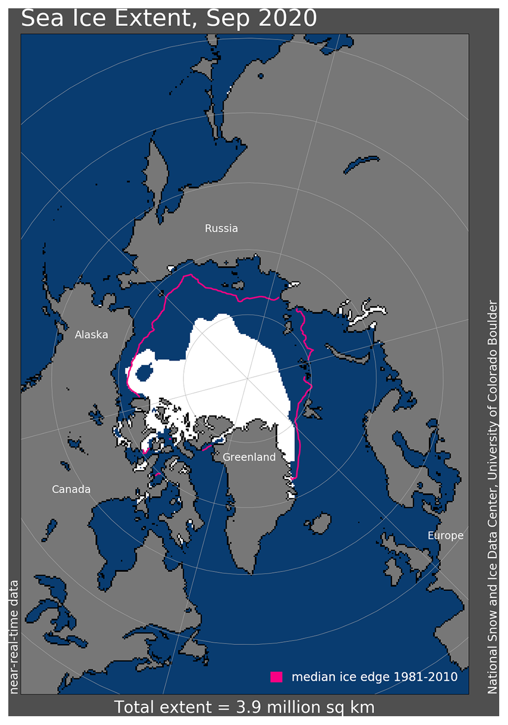
Figure A1Sea ice extent in September 2020. As illustrated, there is no sign of ice in Bering Strait (Fetterer et al., 2017).
B1 EDGAR V6.0 inventories used and sub-categories created
Table B1The 21 EDGAR V6.0 inventories used for the present study regrouped in three different sub-categories.

B2 Graphical representation of the main inventories used
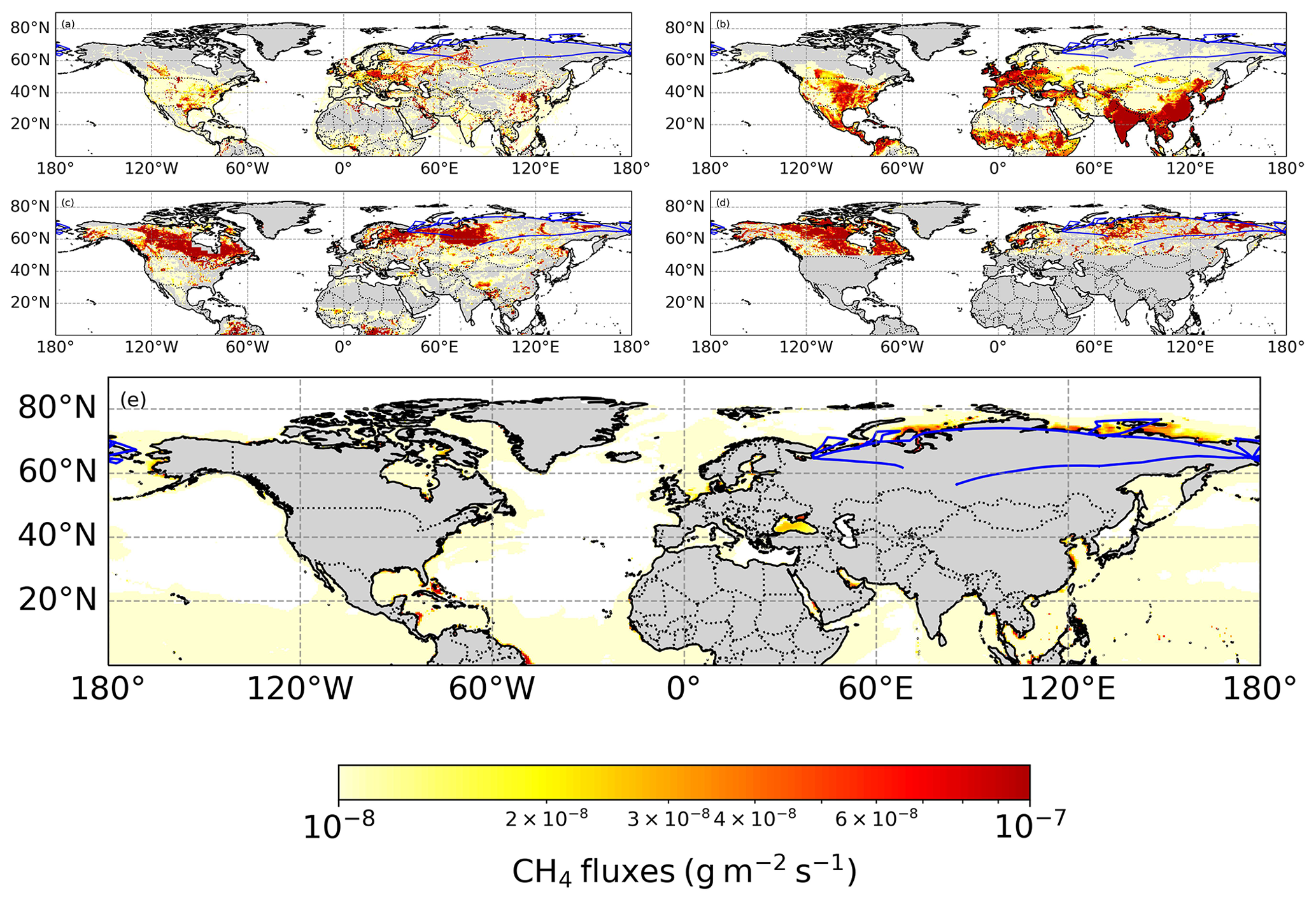
Figure B1(a) Graphical representation of CH4 fluxes due to fossil fuel exploitation as reported in Appendix Table A1 by EDGAR inventories. The trajectory of the campaign is represented by the blue line. (b) Same as (a) for agriculture by EDGAR. (c) Same as (a) for wetlands by ORCHIDEE. (d) Same as (a) for freshwater by bLake4Me and GLWD. (e) Same as (a) for oceans as described in Weber et al. (2019).
Potential emission sensitivity (PES) under 500 m map for flight L3 at 05:01 UTC
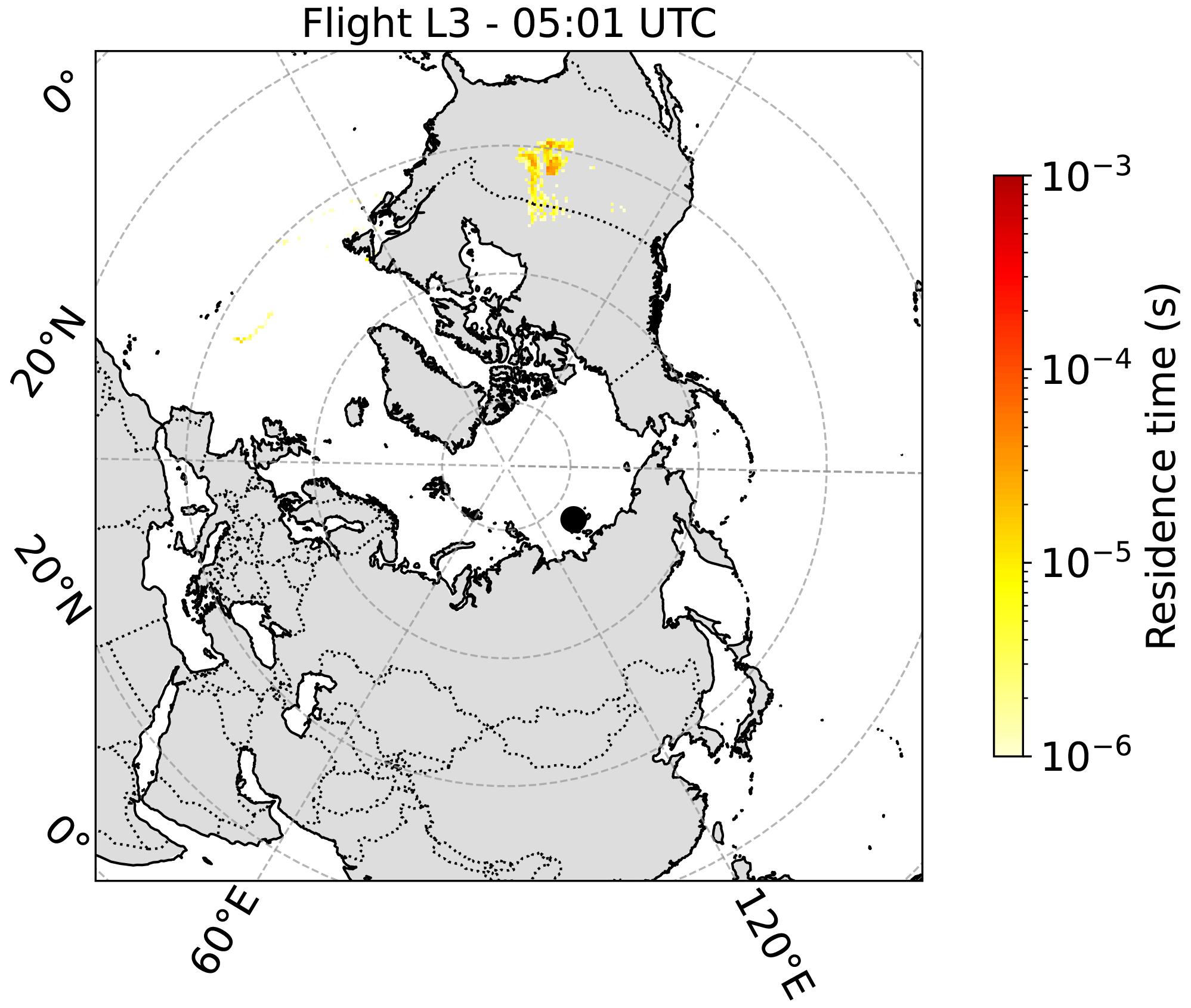
Figure C1The 10 d potential emission sensitivity (PES) with a threshold altitude of 500 m for particles released at 05:01 UTC at an altitude of 5256 m. The black dot represents the position of the receptor.
Tundra around Naryan Mar
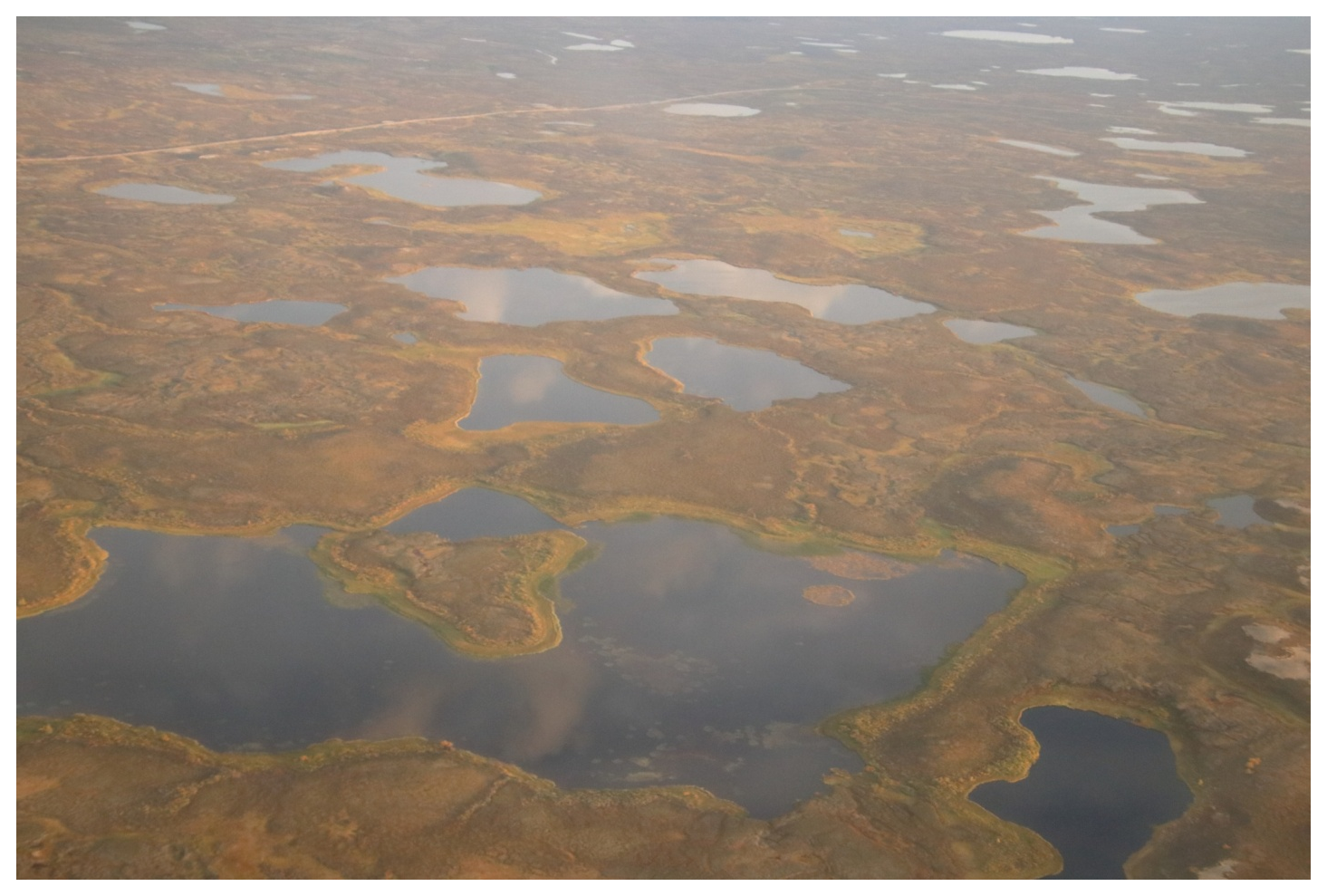
Figure D1An aerial picture of the tundra around Naryan Mar revealing the presence of a huge number of lakes in the region. The picture was provided by Boris D. Belan.
In-flight measurement data are available at https://doi.org/10.5281/zenodo.7642554 (Paris et al., 2023).
CN performed data processing and simulations and analysed the data. JDP designed the study. CN and JDP wrote the first version of the manuscript. AB, SW, and MS helped to perform simulations. BDB, MYA, and SBB designed, organized, and (together with DD, AF, and AK) performed the aircraft campaign and did the trace gas measurements. PN provided CO and O3 data. All contributed to the manuscript.
The contact author has declared that none of the authors has any competing interests.
Publisher’s note: Copernicus Publications remains neutral with regard to jurisdictional claims in published maps and institutional affiliations.
This article is part of the special issue “Pan-Eurasian Experiment (PEEX) – Part II”. It is not associated with a conference.
The aircraft campaign was realized by V. E. Zuev Institute of Atmospheric Optics SB RAS. Data exchange and collaboration were done in the frame of the YAK-AEROSIB MoU. We thank the European Centre for Medium-Range Weather Forecasts (ECMWF) for the provision of ERA-Interim reanalysis data and the FLEXPART development team for the provision of the FLEXPART 9.2 model version. We thank Joel Thanwerdas and Thibaud Thonat for adapting the inventories used in the study. The MEMENTO database is administered by the Kiel Data Management Team at GEOMAR Helmholtz Centre for Ocean Research and supported by the German BMBF project SOPRAN (Surface Ocean Processes in the Anthropocene, http://sopran.pangaea.de, last access: 20 March 2019). The database is accessible through the MEMENTO web page: https://memento.geomar.de (last access: 20 March 2019).
This research has been supported by the Ministry of Science and Higher Education of the Russian Federation (grant no. 075-15-2021-934). Publisher's note: the article processing charges for this publication were not paid by a Russian or Belarusian institution.
This paper was edited by Tanja Schuck and reviewed by David Lowry and one anonymous referee.
Antokhin, P. N., Arshinova, V. G., Arshinov, M. Y., Belan, B. D., Belan, S. B., Davydov, D. K., Ivlev, G. A., Fofonov, A. V., Kozlov, A. V., Paris, J. D., Nedelec, P., Rasskazchikova, T. M., Savkin, D. E., Simonenkov, D. V., Sklyadneva, T. K., and Tolmachev, G. N.: Distribution of Trace Gases and Aerosols in the Troposphere Over Siberia During Wildfires of Summer 2012, J. Geophys. Res-Atmos., 123, 2285–2297, https://doi.org/10.1002/2017JD026825, 2018.
Bartalev, S. A., Belward, A. S., Erchov, D. V., and Isaev, A. S.: A new SPOT4-VEGETATION derived land cover map of Northern Eurasia, Int. J. of Remote. Sens., 24, 1977–1982, https://doi.org/10.1080/0143116031000066297, 2003.
Belan, B. D., Ancellet, G., Andreeva, I. S., Antokhin, P. N., Arshinova, V. G., Arshinov, M. Y., Balin, Y. S., Barsuk, V. E., Belan, S. B., Chernov, D. G., Davydov, D. K., Fofonov, A. V., Ivlev, G. A., Kotel'nikov, S. N., Kozlov, A. S., Kozlov, A. V., Law, K., Mikhal'chishin, A. V., Moseikin, I. A., Nasonov, S. V., Nédélec, P., Okhlopkova, O. V., Ol'kin, S. E., Panchenko, M. V., Paris, J.-D., Penner, I. E., Ptashnik, I. V., Rasskazchikova, T. M., Reznikova, I. K., Romanovskii, O. A., Safatov, A. S., Savkin, D. E., Simonenkov, D. V., Sklyadneva, T. K., Tolmachev, G. N., Yakovlev, S. V., and Zenkova, P. N.: Integrated airborne investigation of the air composition over the Russian sector of the Arctic, Atmos. Meas. Tech., 15, 3941–3967, https://doi.org/10.5194/amt-15-3941-2022, 2022.
Belikov, D., Arshinov, M., Belan, B., Davydov, D., Fofonov, A., Sasakawa, M., and Machida, T.: Analysis of the diurnal,weekly, and seasonal cycles and annual trends in atmospheric CO2 and CH4 at tower network in Siberia from 2005 to 2016, Atmosphere-Basel, 10, 689, https://doi.org/10.3390/atmos10110689, 2019.
Berchet, A., Paris, J. D., Ancellet, G., Law, K. S., Stohl, A., Nédélec, P., Arshinov, M. Y., Belan, B. D., and Ciais, P.: Tropospheric ozone over Siberia in spring 2010: Remote influences and stratospheric intrusion, Tellus B., 65, 1–14, https://doi.org/10.3402/tellusb.v65i0.19688, 2013.
Berchet, A., Pison, I., Chevallier, F., Paris, J.-D., Bousquet, P., Bonne, J.-L., Arshinov, M. Y., Belan, B. D., Cressot, C., Davydov, D. K., Dlugokencky, E. J., Fofonov, A. V., Galanin, A., Lavrič, J., Machida, T., Parker, R., Sasakawa, M., Spahni, R., Stocker, B. D., and Winderlich, J.: Natural and anthropogenic methane fluxes in Eurasia: a mesoscale quantification by generalized atmospheric inversion, Biogeosciences, 12, 5393–5414, https://doi.org/10.5194/bg-12-5393-2015, 2015.
Berchet, A., Bousquet, P., Pison, I., Locatelli, R., Chevallier, F., Paris, J.-D., Dlugokencky, E. J., Laurila, T., Hatakka, J., Viisanen, Y., Worthy, D. E. J., Nisbet, E., Fisher, R., France, J., Lowry, D., Ivakhov, V., and Hermansen, O.: Atmospheric constraints on the methane emissions from the East Siberian Shelf, Atmos. Chem. Phys., 16, 4147–4157, https://doi.org/10.5194/acp-16-4147-2016, 2016.
Berchet, A., Pison, I., Crill, P. M., Thornton, B., Bousquet, P., Thonat, T., Hocking, T., Thanwerdas, J., Paris, J.-D., and Saunois, M.: Using ship-borne observations of methane isotopic ratio in the Arctic Ocean to understand methane sources in the Arctic, Atmos. Chem. Phys., 20, 3987–3998, https://doi.org/10.5194/acp-20-3987-2020, 2020.
Biraud, S., Ciais, P., Ramonet, M., Simmonds, P., Kazan, V., Monfray, P., O'Doherty, S., Spain, T. G., and Jennings, S. G.: European greenhouse gas emissions estimated from continuous atmospheric measurements and radon 222 at Mace Head, Ireland, J. Geophys. Res-Atmos., 105, 1351–1366, https://doi.org/10.1029/1999JD900821, 2000.
Crippa, M., Oreggioni, G., Guizzardi, D., Muntean, M., Schaaf, E., Lo Vullo, E., Solazzo, E., Monforti-Ferrario, F., Olivier, J., and Vignati, E.: Fossil CO2 and GHG emissions of all world countries, Publications Office of the European Union, Luxembourg, https://doi.org/10.2760/687800, 2019.
Dlugokencky, E., Mund, J., Crotwell, A., Crotwell, M., and Thoning, K.: Atmospheric Carbon Dioxide Dry Air Mole Fractions, NOAA GML Carbon Cycle Cooperative Global Air Sampling Network [data set], https://doi.org/10.15138/wkgj-f215, 2021a.
Dlugokencky, E., Mund, J., Crotwell, A., Crotwell, M., and Thoning, K.: Atmospheric Methane Dry Air Mole Fractions, NOAA GML Carbon Cycle Cooperative Global Air Sampling Network [data set], https://doi.org/10.15138/wkgj-f215, 2021b.
Dlugokencky, E., Mund, J., Crotwell, A., Crotwell, M., and Thoning, K: Atmospheric methane from quasi-continuous measurements at Barrow, Alaska and Mauna Loa, Hawaii, 1986–2020, Version: 2021-03, NOAA GML Carbon Cycle Cooperative Global Air Sampling Network [data set], https://doi.org/10.15138/ve0c-be70, 2021c.
Elder, C. D., Thompson, D. R., Thorpe, A. K., Hanke, P., Walter Anthony, K. M., and Miller, C. E.: Airborne Mapping Reveals Emergent Power Law of Arctic Methane Emissions, Geophys. Res. Lett., 47, e2019GL085707, https://doi.org/10.1029/2019GL085707, 2020.
Etiope, G., Ciotoli, G., Schwietzke, S., and Schoell, M.: Gridded maps of geological methane emissions and their isotopic signature, Earth Syst. Sci. Data, 11, 1–22, https://doi.org/10.5194/essd-11-1-2019, 2019.
Etminan, M., Myhre, G., Highwood, E. J., and Shine, K. P.: Radiative forcing of carbon dioxide, methane, and nitrous oxide: A significant revision of the methane radiative forcing, Geophys. Res. Lett., 43, 12614–12623, https://doi.org/10.1002/2016GL071930, 2016.
Fetterer, F., Knowles, K., Meier, W. N., Savoie, M., and Windnagel., A. K.: Sea Ice Index, Version 3. [Sea Ice Extent], National Snow and Ice Data Center (NSIDC) [data set], https://doi.org/10.7265/N5K072F8, 2017.
Fleming, Z. L., Monks, P. S., and Manning, A. J.: Review: Untangling the influence of air-mass history in interpreting observed atmospheric composition, Atmos. Res., 104-105, 1–39, https://doi.org/10.1016/j.atmosres.2011.09.009, 2012.
Friedlingstein, P., O'Sullivan, M., Jones, M. W., Andrew, R. M., Hauck, J., Olsen, A., Peters, G. P., Peters, W., Pongratz, J., Sitch, S., Le Quéré, C., Canadell, J. G., Ciais, P., Jackson, R. B., Alin, S., Aragão, L. E. O. C., Arneth, A., Arora, V., Bates, N. R., Becker, M., Benoit-Cattin, A., Bittig, H. C., Bopp, L., Bultan, S., Chandra, N., Chevallier, F., Chini, L. P., Evans, W., Florentie, L., Forster, P. M., Gasser, T., Gehlen, M., Gilfillan, D., Gkritzalis, T., Gregor, L., Gruber, N., Harris, I., Hartung, K., Haverd, V., Houghton, R. A., Ilyina, T., Jain, A. K., Joetzjer, E., Kadono, K., Kato, E., Kitidis, V., Korsbakken, J. I., Landschützer, P., Lefèvre, N., Lenton, A., Lienert, S., Liu, Z., Lombardozzi, D., Marland, G., Metzl, N., Munro, D. R., Nabel, J. E. M. S., Nakaoka, S.-I., Niwa, Y., O'Brien, K., Ono, T., Palmer, P. I., Pierrot, D., Poulter, B., Resplandy, L., Robertson, E., Rödenbeck, C., Schwinger, J., Séférian, R., Skjelvan, I., Smith, A. J. P., Sutton, A. J., Tanhua, T., Tans, P. P., Tian, H., Tilbrook, B., van der Werf, G., Vuichard, N., Walker, A. P., Wanninkhof, R., Watson, A. J., Willis, D., Wiltshire, A. J., Yuan, W., Yue, X., and Zaehle, S.: Global Carbon Budget 2020, Earth Syst. Sci. Data, 12, 3269–3340, https://doi.org/10.5194/essd-12-3269-2020, 2020.
Fujita, R., Morimoto, S., Maksyutov, S., Kim, H.-S., Arshinov, M., Brailsford, G., Aoki, S., and Nakazawa, T.: Global and Regional CH4 Emissions for 1995–2013 Derived From Atmospheric CH4, δ13C-CH4, and δD-CH4 Observations and a Chemical Transport Model. J. Geophys. Res.-Atmos., 125, e2020JD032903, https://doi.org/10.1029/2020JD032903, 2020.
Gerbig, C., Lin, J. C., Wofsy, S. C., Daube, B. C., Andrews, A. E., Stephens, B. B., Bakwin, P. S., and Grainger, C. A.: Toward constraining regional-scale fluxes of CO2 with atmospheric observations over a continent: 2. Analysis of COBRA data using a receptor-oriented framework, J. Geophys. Res., 108, 4757, https://doi.org/10.1029/2003JD003770, 2003.
Global Coal Mine Tracker: Global Energy Monitor, https://globalenergymonitor.org/projects/global-coal-mine-tracker/ (last access: 19 September 2021), 2022.
Global Fossil Infrastructure Tracker: Global Energy Monitor: https://globalenergymonitor.org/projects/global-fossil-infrastructure-tracker/tracker-map/ (last access: 19 September 2021), 2022.
Hazan, L., Tarniewicz, J., Ramonet, M., Laurent, O., and Abbaris, A.: Automatic processing of atmospheric CO2 and CH4 mole fractions at the ICOS Atmosphere Thematic Centre, Atmos. Meas. Tech., 9, 4719–4736, https://doi.org/10.5194/amt-9-4719-2016, 2016.
Hersbach, H., Bell, B., Berrisford, P., Biavati, G., Horányi, A., Muñoz Sabater, J., Nicolas, J., Peubey, C., Radu, R., Rozum, I., Schepers, D., Simmons, A., Soci, C., Dee, D., and Thépaut, J-N.: ERA5 hourly data on single levels from 1979 to present, Copernicus Climate Change Service (C3S) Climate Data Store (CDS) [data set], https://doi.org/10.24381/cds.adbb2d47 (last access: 4 October 2021), 2018.
Kirschke, S., Bousquet, P., Ciais, P., Saunois, M., Canadell, J. G., Dlugokencky, E. J., Bergamaschi, P., Bergmann, D., Blake, D. R., Bruhwiler, L., Cameron-Smith, P., Castaldi, S., Chevallier, F., Feng, L., Fraser, A., Heimann, M., Hodson, E. L., Houweling, S., Josse, B., Fraser, P. J., Krummel, P. B., Lamarque, J. F., Langenfelds, R. L., Le Quéré, C., Naik, V., O'doherty, S., Palmer, P. I., Pison, I., Plummer, D., Poulter, B., Prinn, R. G., Rigby, M., Ringeval, B., Santini, M., Schmidt, M., Shindell, D. T., Simpson, I. J., Spahni, R., Steele, L. P., Strode, S. A., Sudo, K., Szopa, S., Van Der Werf, G. R., Voulgarakis, A., Van Weele, M., Weiss, R. F., Williams, J. E., and Zeng, G.: Three decades of global methane sources and sinks, Nat. Geosci., 6, 813–823, https://doi.org/10.1038/ngeo1955, 2013.
Kock, A. and Bange, H.: Counting the Ocean's Greenhouse Gas Emissions, Eos, 96, 10–13, https://doi.org/10.1029/2015EO023665, 2015.
Lan, X., Nisbet, E. G., Dlugokencky, E. J., and Michel, S. E.: What do we know about the global methane budget? Results from four decades of atmospheric CH4 observations and the way forward, Philos. T. R. Soc. A, 379, 20200440, https://doi.org/10.1098/rsta.2020.0440, 2021.
Lehner, B. and Döll, P.: Development and validation of a global database of lakes, reservoirs and wetlands, J. Hydrol., 296, 1–22515, https://doi.org/10.1016/j.jhydrol.2004.03.028, 2004.
Masson-Delmotte, V., Zhai, P., Pirani, A., Connors, S. L., Péan, C., Berger, S., Caud, N., Chen, Y., Goldfarb, L., Gomis, M. I., Huang, M., Leitzell, K., Lonnoy, E., Matthews, J. B. R., Maycock, T. K., Waterfield, T., Yelekçi, O., Yu, R., and Zhou, B. (Eds.): Climate Change 2021: The Physical Science Basis. Contribution of Working Group I to the Sixth Assessment Report of the Intergovernmental Panel on Climate Change, Cambridge Univerity Press, Cambridge, in press, 2021.
Matthews, E., Johnson, M. S., Genovese, V., Du, J., and Bastviken, D.: Methane emission from high latitude lakes: methane-centric lake classification and satellite-driven annual cycle of emissions, Sci. Rep-UK, 10, 1–9, https://doi.org/10.1038/s41598-020-68246-1, 2020.
Melton, J. R., Wania, R., Hodson, E. L., Poulter, B., Ringeval, B., Spahni, R., Bohn, T., Avis, C. A., Beerling, D. J., Chen, G., Eliseev, A. V., Denisov, S. N., Hopcroft, P. O., Lettenmaier, D. P., Riley, W. J., Singarayer, J. S., Subin, Z. M., Tian, H., Zürcher, S., Brovkin, V., van Bodegom, P. M., Kleinen, T., Yu, Z. C., and Kaplan, J. O.: Present state of global wetland extent and wetland methane modelling: conclusions from a model inter-comparison project (WETCHIMP), Biogeosciences, 10, 753–788, https://doi.org/10.5194/bg-10-753-2013, 2013.
Oltmans, S. J. and Levy, H.: Surface ozone measurements from a global network, Atmos. Environ., 28, 9–24, https://doi.org/10.1016/1352-2310(94)90019-1, 1994.
Paris, J. D., Ciais, P., Nédélec, P., Ramonet, M., Belan, B. D., Arshinov, M. Y., Golitsyn, G. S., Granberg, I., Stohl, A., Cayez, G., Athier, G., Boumard, F., and Cousin, J. M.: The YAK-AEROSIB transcontinental aircraft campaigns: New insights on the transport of CO2, CO and O3 across Siberia, Tellus B, 60, 551–568, https://doi.org/10.1111/j.1600-0889.2008.00369.x, 2008.
Paris, J.-D., Stohl, A., Nédélec, P., Arshinov, M. Yu., Panchenko, M. V., Shmargunov, V. P., Law, K. S., Belan, B. D., and Ciais, P.: Wildfire smoke in the Siberian Arctic in summer: source characterization and plume evolution from airborne measurements, Atmos. Chem. Phys., 9, 9315–9327, https://doi.org/10.5194/acp-9-9315-2009, 2009.
Paris, J.-D., Ciais, P., Nédélec, P., Stohl, A., Belan, B. D., Arshinov, M. Y., Carouge, C., Golitsyn, G. S., and Granberg, I. G.: New Insights on the Chemical Composition of the Siberian Air Shed From The Yak-Aerosib Aircraft Campaigns, B. Am. Meteorol. Soc., 91, 625–642, https://doi.org/10.1175/2009BAMS2663.1, 2010a.
Paris, J.-D., Stohl, A., Ciais, P., Nédélec, P., Belan, B. D., Arshinov, M. Yu., and Ramonet, M.: Source-receptor relationships for airborne measurements of CO2, CO and O3 above Siberia: a cluster-based approach, Atmos. Chem. Phys., 10, 1671–1687, https://doi.org/10.5194/acp-10-1671-2010, 2010b.
Paris, J.-D., Belan, B. D., Arshinov, M. Yu., Nédélec, P., Belan, S. B., Davydov, D., Fofonov, A., and Kozlov, A.: Arctic campaign 2020 – YAK-AEROSIB – trace gas measurements, Zenodo [data set], https://doi.org/10.5281/zenodo.7642554, 2023.
Petäjä, T., Ganzei, K. S., Lappalainen, H. K., Tabakova, K., Makkonen, R., Räisänen, J., Chalov, S., Kulmala, M., Zilitinkevich, S., Baklanov, P. Y., Shakirov, R. B., Mishina, N. V., Egidarev, E. G., and Kondrat'ev, I. I.: Research agenda for the Russian Far East and utilization of multi-platform comprehensive environmental observations, Int. J. Digit. Earth., 14, 311–337, https://doi.org/10.1080/17538947.2020.1826589, 2021.
Pisso, I., Sollum, E., Grythe, H., Kristiansen, N. I., Cassiani, M., Eckhardt, S., Arnold, D., Morton, D., Thompson, R. L., Groot Zwaaftink, C. D., Evangeliou, N., Sodemann, H., Haimberger, L., Henne, S., Brunner, D., Burkhart, J. F., Fouilloux, A., Brioude, J., Philipp, A., Seibert, P., and Stohl, A.: The Lagrangian particle dispersion model FLEXPART version 10.4, Geosci. Model Dev., 12, 4955–4997, https://doi.org/10.5194/gmd-12-4955-2019, 2019.
Platt, S. M., Eckhardt, S., Ferré, B., Fisher, R. E., Hermansen, O., Jansson, P., Lowry, D., Nisbet, E. G., Pisso, I., Schmidbauer, N., Silyakova, A., Stohl, A., Svendby, T. M., Vadakkepuliyambatta, S., Mienert, J., and Lund Myhre, C.: Methane at Svalbard and over the European Arctic Ocean, Atmos. Chem. Phys., 18, 17207–17224, https://doi.org/10.5194/acp-18-17207-2018, 2018.
Ringeval, B., Decharme, B., Piao, S. L., Ciais, P., Papa, F., de Noblet-Ducoudré, N., Prigent, C., Friedlingstein, P., Gouttevin, I., Koven, C., and Ducharne, A.: Modelling sub-grid wetland in the ORCHIDEE global land surface model: evaluation against river discharges and remotely sensed data, Geosci. Model Dev., 5, 941–962, https://doi.org/10.5194/gmd-5-941-2012, 2012.
Rosentreter, J. A., Borges, A. V., Deemer, B. R., Holgerson, M. A., Liu, S., Song, C., Melack, J., Raymond, P. A., Duarte, C. M., Allen, G. H., Olefeldt, D., Poulter, B., Battin, T. I., and Eyre, B. D.: Half of global methane emissions come from highly variable aquatic ecosystem sources, Nat. Geosci., 14, 225–230, https://doi.org/10.1038/s41561-021-00715-2, 2021.
Ruppel, C.: Permafrost-Associated Gas Hydrate: Is It Really Approximately 1 % of the Global System?, J. Chem. Eng. Data., 60, 429–436, https://doi.org/10.1021/je500770m, 2015.
Sasakawa, M., Shimoyama, K., Machida, T., Tsuda, N., Suto, H., Arshinov, M., Davydov, D., Fofonov, A., Krasnov, O., Saeki, T., Koyama, Y., and Maksyutov, S.: Continuous measurements of methane from a tower network over Siberia, Tellus B, 62, 403–416, https://doi.org/10.1111/j.1600-0889.2010.00494.x, 2010.
Sasakawa, M., Machida, T., Ishijima, K., Arshinov, M., Patra, P. K., Ito, A., Aoki, S., and Petrov, V.: Temporal characteristics of CH4 vertical profiles observed in the West Siberian Lowland over Surgut from 1993 to 2015 and Novosibirsk from 1997 to 2015, J. Geophys. Res.-Atmos., 122, 11,261–11,273, https://doi.org/10.1002/2017JD026836, 2017.
Saunois, M., Bousquet, P., Poulter, B., Peregon, A., Ciais, P., Canadell, J. G., Dlugokencky, E. J., Etiope, G., Bastviken, D., Houweling, S., Janssens-Maenhout, G., Tubiello, F. N., Castaldi, S., Jackson, R. B., Alexe, M., Arora, V. K., Beerling, D. J., Bergamaschi, P., Blake, D. R., Brailsford, G., Brovkin, V., Bruhwiler, L., Crevoisier, C., Crill, P., Covey, K., Curry, C., Frankenberg, C., Gedney, N., Höglund-Isaksson, L., Ishizawa, M., Ito, A., Joos, F., Kim, H.-S., Kleinen, T., Krummel, P., Lamarque, J.-F., Langenfelds, R., Locatelli, R., Machida, T., Maksyutov, S., McDonald, K. C., Marshall, J., Melton, J. R., Morino, I., Naik, V., O'Doherty, S., Parmentier, F.-J. W., Patra, P. K., Peng, C., Peng, S., Peters, G. P., Pison, I., Prigent, C., Prinn, R., Ramonet, M., Riley, W. J., Saito, M., Santini, M., Schroeder, R., Simpson, I. J., Spahni, R., Steele, P., Takizawa, A., Thornton, B. F., Tian, H., Tohjima, Y., Viovy, N., Voulgarakis, A., van Weele, M., van der Werf, G. R., Weiss, R., Wiedinmyer, C., Wilton, D. J., Wiltshire, A., Worthy, D., Wunch, D., Xu, X., Yoshida, Y., Zhang, B., Zhang, Z., and Zhu, Q.: The global methane budget 2000–2012, Earth Syst. Sci. Data, 8, 697–751, https://doi.org/10.5194/essd-8-697-2016, 2016.
Saunois, M., Stavert, A. R., Poulter, B., Bousquet, P., Canadell, J. G., Jackson, R. B., Raymond, P. A., Dlugokencky, E. J., Houweling, S., Patra, P. K., Ciais, P., Arora, V. K., Bastviken, D., Bergamaschi, P., Blake, D. R., Brailsford, G., Bruhwiler, L., Carlson, K. M., Carrol, M., Castaldi, S., Chandra, N., Crevoisier, C., Crill, P. M., Covey, K., Curry, C. L., Etiope, G., Frankenberg, C., Gedney, N., Hegglin, M. I., Höglund-Isaksson, L., Hugelius, G., Ishizawa, M., Ito, A., Janssens-Maenhout, G., Jensen, K. M., Joos, F., Kleinen, T., Krummel, P. B., Langenfelds, R. L., Laruelle, G. G., Liu, L., Machida, T., Maksyutov, S., McDonald, K. C., McNorton, J., Miller, P. A., Melton, J. R., Morino, I., Müller, J., Murguia-Flores, F., Naik, V., Niwa, Y., Noce, S., O'Doherty, S., Parker, R. J., Peng, C., Peng, S., Peters, G. P., Prigent, C., Prinn, R., Ramonet, M., Regnier, P., Riley, W. J., Rosentreter, J. A., Segers, A., Simpson, I. J., Shi, H., Smith, S. J., Steele, L. P., Thornton, B. F., Tian, H., Tohjima, Y., Tubiello, F. N., Tsuruta, A., Viovy, N., Voulgarakis, A., Weber, T. S., van Weele, M., van der Werf, G. R., Weiss, R. F., Worthy, D., Wunch, D., Yin, Y., Yoshida, Y., Zhang, W., Zhang, Z., Zhao, Y., Zheng, B., Zhu, Q., Zhu, Q., and Zhuang, Q.: The Global Methane Budget 2000–2017, Earth Syst. Sci. Data, 12, 1561–1623, https://doi.org/10.5194/essd-12-1561-2020, 2020.
Seibert, P. and Frank, A.: Source-receptor matrix calculation with a Lagrangian particle dispersion model in backward mode, Atmos. Chem. Phys., 4, 51–63, https://doi.org/10.5194/acp-4-51-2004, 2004.
Shakhova, N., Semiletov, I., Salyuk, A., Yusupov, V., Kosmach, D., and Gustafsson, O.: Extensive Methane Venting to the Atmosphere from Sediments of the East Siberian Arctic Shelf, Science, 327, 1246–1250, https://doi.org/10.1126/science.1182221, 2010.
Skorokhod, A. I., Berezina, E. V., Moiseenko, K. B., Elansky, N. F., and Belikov, I. B.: Benzene and toluene in the surface air of northern Eurasia from TROICA-12 campaign along the Trans-Siberian Railway, Atmos. Chem. Phys., 17, 5501–5514, https://doi.org/10.5194/acp-17-5501-2017, 2017.
Steinbach, J., Holmstrand, H., Shcherbakova, K., Kosmach, D., Brüchert, V., Shakhova, N., Salyuk, A., Sapart, C. J., Chernykh, D., Noormets, R., Semiletov, I., and Gustafsson, O.: Source ap- portionment of methane escaping the subsea permafrost system in the outer Eurasian Arctic Shelf, P. Natl. Acad. Sci. USA, 118, e2019672118, https://doi.org/10.1073/pnas.2019672118, 2021.
Stöckli, R., Vermote, E., Saleous, N., Simmon, R., and Herring, D.: The Blue Marble Next Generation-A true color earth dataset including seasonal dynamics from MODIS, published by the NASA Earth Observatory, https://earthobservatory.nasa.gov/ContentFeature/BlueMarble/bmng.pdf (last access: 27 April 2022), 2005.
Stohl, A. and Thomson, D. J.: A Density Correction for Lagrangian Particle Dispersion Models, Bound-Lay. Meteorol., 90, 155–167, https://doi.org/10.1023/A:1001741110696, 1999.
Stohl, A., Wotawa, G., Seibert, P., and Kromp-Kolb, H.: Interpolation Errors in Wind Fields as a Function of Spatial and Temporal Resolution and Their Impact on Different Types of Kinematic Trajectories, J. Appl. Meteorol., 34, 2149–2165, https://doi.org/10.1175/1520-0450(1995)034<2149:IEIWFA>2.0.CO;2, 1995.
Stohl, A., Hittenberger, M., and Wotawa, G.: Validation of the lagrangian particle dispersion model FLEXPART against large-scale tracer experiment data, Atmos. Environ., 32, 4245–4264, https://doi.org/10.1016/S13522310(98)001848, 1998.
Stohl, A., Forster, C., Frank, A., Seibert, P., and Wotawa, G.: Technical note: The Lagrangian particle dispersion model FLEXPART version 6.2, Atmos. Chem. Phys., 5, 2461–2474, https://doi.org/10.5194/acp-5-2461-2005, 2005.
Tan, Z., Zhuang, Q., and Walter Anthony, K.: Modeling methane emissions from arctic lakes: Model development and site-level study, J. Adv. Model. Earth. Sy., 7, 459–483, https://doi.org/10.1002/2014MS000344, 2015.
Thonat, T., Saunois, M., Bousquet, P., Pison, I., Tan, Z., Zhuang, Q., Crill, P. M., Thornton, B. F., Bastviken, D., Dlugokencky, E. J., Zimov, N., Laurila, T., Hatakka, J., Hermansen, O., and Worthy, D. E. J.: Detectability of Arctic methane sources at six sites performing continuous atmospheric measurements, Atmos. Chem. Phys., 17, 8371–8394, https://doi.org/10.5194/acp-17-8371-2017, 2017.
Thornton, B. F., Geibel, M. C., Crill, P. M., Humborg, C., and Mörth, C. M.: Methane fluxes from the sea to the atmosphere across the Siberian shelf seas, Geophys. Res. Lett., 43, 5869–5877, https://doi.org/10.1002/2016GL068977, 2016.
Thornton, B. F., Prytherch, J., Andersson, K., Brooks, I. M., Salisbury, D., Tjernström, M., and Crill, P. M.: Shipborne eddy covariance observations of methane fluxes constrain Arctic sea emissions, Sci. Adv., 6, 1–11, https://doi.org/10.1126/sciadv.aay7934, 2020.
Turetsky, M. R., Jones, M., Walter Anthony, K., Olefeldt, D., Schuur, E. A., Koven, C., Mcguire, A. D., and Grosse, G.: Permafrost collapse is accelerating carbon release, Nature, 569, 32–24, 2019.
van der Werf, G. R., Randerson, J. T., Giglio, L., van Leeuwen, T. T., Chen, Y., Rogers, B. M., Mu, M., van Marle, M. J. E., Morton, D. C., Collatz, G. J., Yokelson, R. J., and Kasibhatla, P. S.: Global fire emissions estimates during 1997–2016, Earth Syst. Sci. Data, 9, 697–720, https://doi.org/10.5194/essd-9-697-2017, 2017.
Wania, R., Melton, J. R., Hodson, E. L., Poulter, B., Ringeval, B., Spahni, R., Bohn, T., Avis, C. A., Chen, G., Eliseev, A. V., Hopcroft, P. O., Riley, W. J., Subin, Z. M., Tian, H., van Bodegom, P. M., Kleinen, T., Yu, Z. C., Singarayer, J. S., Zürcher, S., Lettenmaier, D. P., Beerling, D. J., Denisov, S. N., Prigent, C., Papa, F., and Kaplan, J. O.: Present state of global wetland extent and wetland methane modelling: methodology of a model inter-comparison project (WETCHIMP), Geosci. Model Dev., 6, 617–641, https://doi.org/10.5194/gmd-6-617-2013, 2013.
Weber, T., Wiseman, N. A., and Kock, A.: Global ocean methane emissions dominated by shallow coastal waters, Nat. Commun., 10, 1–10, https://doi.org/10.1038/s41467-019-12541-7, 2019.
Wik, M., Thornton, B. F., Bastviken, D., Uhlbäck, J., and Crill, P. M.: Biased sampling of methane release from northern lakes: A problem for extrapolation, Geophys. Res. Lett., 43, 1256–1262, https://doi.org/10.1002/2015GL066501, 2016.
World Meteorological Organization (WMO): Greenhouse Gas Bulletin No.17: The State of Greenhouse Gases in the Atmosphere Based on Global Observations through 2020, https://public.wmo.int/en/media/press-release/greenhouse-gas-bulletin-another-year-another-record (last access: 7 January 2022), 2021.
AK-Aerosib Measurements: YAK-AEROSIB, https://yak.aeris-data.fr/welcome/measurements/, last access: 19 September 2021.
Zhang, Z., Fluet-Chouinard, E., Jensen, K., McDonald, K., Hugelius, G., Gumbricht, T., Carroll, M., Prigent, C., Bartsch, A., and Poulter, B.: Development of the global dataset of Wetland Area and Dynamics for Methane Modeling (WAD2M), Earth Syst. Sci. Data, 13, 2001–2023, https://doi.org/10.5194/essd-13-2001-2021, 2021.
- Abstract
- Introduction
- Methods
- Results
- Conclusion
- Appendix A: Additional material concerning CO2 enhancements at low altitude in eastern Siberia
- Appendix B: Additional material on inventories
- Appendix C: Additional material concerning flight L3 characterization
- Appendix D: Additional material concerning CH4 freshwater enhancements in the Naryan Mar region
- Data availability
- Author contributions
- Competing interests
- Disclaimer
- Special issue statement
- Acknowledgements
- Financial support
- Review statement
- References