the Creative Commons Attribution 4.0 License.
the Creative Commons Attribution 4.0 License.
 | 14 Feb 2023
On the global relationship between polarimetric radio occultation differential phase shift and ice water content
Estel Cardellach
F. Joseph Turk
The Radio Occultations and Heavy Precipitation (ROHP) experiment aboard the Spanish PAZ satellite was deployed in 2018 with the objective of demonstrating the ability of the polarimetric radio occultation measurement (PRO) concept in detecting rain (liquid-phase precipitation). Analysis of these data has also demonstrated the ability of PRO to detect horizontally oriented frozen-phase precipitation. To verify these observations, a global climatological comparison is performed using the CloudSat (94 GHz) radar as a reference for different heights and taking into account the radio occultation (limb-based) viewing geometry. A robust relationship (e.g., high correlation coefficient) is found between the polarimetric radio occultation observable differential phase shift (ΔΦ) and the integrated ice water content (IWC) along the rays, globally, and for heights above freezing level. PAZ observations capture the major precipitation features and the signatures of the Intertropical Convergence Zone. The correlation coefficients maximize for tropical oceans, for a range of heights between 5 and 12 km. The ratios between ΔΦ and along-ray integrated IWC mean that climatologies are found to be within the range 0.03–0.09 mm kg−1 m2, although uncertainty due to the IWC retrieval algorithm must be noted. Further evaluation of the ratios with single-particle forward-scattering simulations indicate that the scattering by frozen hydrometeors with a combination of effective densities, axis ratios, and tilt angle distribution yield results that agree well with the observations. Overall, the global climatological results obtained in this study show the presence of horizontally oriented particles across the whole globe and for a wide range of height layers.
- Article
(9379 KB) - Full-text XML
- BibTeX
- EndNote


The Radio Occultations and Heavy Precipitation (ROHP) experiment aboard the Spanish PAZ satellite (Cardellach et al., 2014) has demonstrated the ability of the polarimetric radio occultation (PRO) technique to complement well-established RO processing techniques (e.g., Kursinski et al., 1997) with the detection of heavy precipitation (Cardellach et al., 2019; Padullés et al., 2022). The detection is based on the total differential phase shift (ΔΦ) accumulated along the RO ray paths, traveling from the Global Positioning System (GPS) satellite emitter to the dual linearly polarized (H, V) receiver on the PAZ low Earth orbiter (LEO). Being a limb-sounding technique, the rays travel through deeper layers of the atmosphere as the occultation advances, penetrating into the layers where clouds and precipitation are expected. This differential polarimetric-phase measurement, in units of length, is set as the primary observable for PRO. It depends on the hydrometeors encountered along the rays as follows (Cardellach et al., 2014):
where Kdp is the differential phase shift, and L is the traveled distance. The Kdp is defined as follows:
where λ is the wavelength (i.e., in the case of L-band GPS signals, λ=0.192 m, corresponding to 1.575 GHz), Shh,vv are the co-polar components of the scattering amplitude matrix, and N(D) is the particle size distribution as a function of the equivalent particle diameter, D, i.e., the diameter of a sphere having the same mass.
Kdp contains the dependence of PRO observable on a series of microphysics parameters, such as the size, the shape, and the number of hydrometeors. The scattering amplitude matrix (S; 2×2) provides information on the scattered field after propagating through an ensemble of hydrometeors. It depends on the shape and type of the hydrometeors (raindrops, pristine ice crystals, aggregate of ice particles, etc.). The dependence on the shape is often expressed in terms of the axis ratio, i.e., the ratio between the two main axis of the particle. For a perfectly spherical particle, . Kdp also depends on the size of the hydrometeors. This dependence on the size is proportional to its volume, and therefore it is affected by the third moment of the N(D). The water content (WC) is also affected by the third moment of N(D) as follows (e.g., Bringi and Chandrasekar, 2001):
where ρw,i is the density, typically of water or ice. Therefore, it is expected that a relationship exists between Kdp and WC. In fact, the use of Kdp to retrieve WC has been attempted before, for rain (e.g., Jameson, 1985) and for ice (e.g., Vivekanandan et al., 1994; Ryzhkov et al., 1998; Bukovčić et al., 2018; Nguyen et al., 2019), using radar at different frequencies ranging from the S to K bands. However, in the case of ice and snow, there are additional factors that must be taken into account, namely the percentage of horizontally oriented particles with respect to those that are randomly oriented, the effective density, and the shape and composition (i.e., dielectric constant of the ice/air media). In the case that all particles were randomly oriented, Kdp would cancel out, regardless of the amount of WC.
The shape and orientation of ice particles have a direct relationship with the lifecycle of precipitation (e.g., Gong et al., 2020). Furthermore, knowledge of shape and orientation is crucial for space-based retrievals of, for example, total ice water paths (e.g., Kaur et al., 2022) and could help in the assimilation of passive microwave data in the all-sky assimilation schemes (e.g., Barlakas et al., 2021). In this regard, PRO observations have the potential to help constrain the orientation of the hydrometeors globally, with high vertical resolution. Other limb-sounding techniques, such as the Microwave Limb Sounder (MLS), have previously been used to sense ice particles (e.g., Wu et al., 2009) and constrain their orientation (e.g., Davis et al., 2005), but the MLS vertical resolution is low.
In Padullés et al. (2022), the authors showed that the presence of horizontally oriented frozen particles is required in order to explain some of the PAZ PRO observations. In this new paper, we carry out an extensive analysis of the global relationships between ice water content (IWC) and ΔΦ. To do so, a synthetic radio occultation mission is simulated based on ice water properties provided by the CloudSat data products between 2006–2016. That is, a set of actual radio occultation rays are artificially placed, overlaying the CloudSat curtain-like observations, continuously thorough the whole period. In this way, the CloudSat observations, like radar reflectivity, and their retrievals, like IWC, can be analyzed as if they were observed in RO geometry. The statistics gathered from these observations would be equivalent to any other RO mission if this were able to measure such quantities.
This strategy arises from the fact that there are no coincident observations between the CloudSat and PAZ due to different orbit parameters. However, the artificially generated products enable us to compare, in a statistical or climatological way, the PAZ ΔΦ observations with retrievals from CloudSat, such as the IWC.
In this paper, we focus on the spatial correlations between the IWC as would have been sensed by RO geometries in CloudSat measured backgrounds and the ΔΦ from PAZ. If these two quantities are related, the spatial patterns should agree, and the correlation should be high. This paper is therefore structured as follows: in Sect. 2 the artificial products based on CloudSat retrievals and actual RO geometries are described. In Sect. 3, the correlations and relationship between the actual PAZ observations and the generated products are investigated. Finally, in Sect. 4, forward-scattering simulations are used to validate and contextualize the relationships found in the previous section. The paper ends with a discussion on the findings.
The CloudSat satellite was launched in 28 April 2006 and was regularly providing observations until August 2020. It orbits at an approximate height of 715 km in a polar orbit (inclination of 98.2∘), with an equatorial crossing time of about 01:30 and 13:30 LT (local time). It carries a Cloud Profiling Radar (CPR) operating at 94 GHz (W band), aiming at observing and characterizing clouds (Stephens et al., 2008). Its high-frequency radar is particularly good at sensing the frozen part of clouds and precipitation, whereas it has problems with penetrating to the lower altitudes in the deepest convective regions of precipitating systems (e.g., Battaglia et al., 2007). The parameters observed and retrieved from CloudSat, of interest for this study, consist of the radar reflectivity (Ze) in the 2B-GEOPROF product (Marchand et al., 2008), the IWC retrievals from the DARDAR product (Delanoë and Hogan, 2010) version 3 (Cazenave et al., 2019), and the IWC and particle size distribution parameters (Nt and σ) in the 2B-CWC-RO product (Austin et al., 2009). Auxiliary thermodynamic parameters such as temperature and humidity have been obtained from the European Centre for Medium-Range Weather Forecasts (ECMWF) model and provided along the IWC retrievals. All these parameters are obtained with a vertical resolution of 240 m from the surface up to 25–30 km. Since the aim of this study is a comparison with the PRO observations from PAZ, these parameters are transformed to the RO observing frame, as defined below.
In brief, radio occultation observations consist of a low Earth orbiter (LEO) tracking a Global Navigation Satellite System (GNSS)-emitted signal while it is occulting behind the Earth's horizon (e.g., Kursinski et al., 1997; Hajj et al., 2002). This results in electromagnetic waves from GNSS crossing the different layers of the atmosphere tangentially with respect to Earth's surface, which is commonly known as a limb-sounding observation. One implication of this kind of measurement is that rays cross a long portion of the atmosphere, becoming longer as rays approach the surface. In fact, when rays penetrate below 20 km (the region where clouds are expected), then their traveled distance can be as large as ∼800 km. In the particular case of PRO, this has been discussed in Turk et al. (2021). Therefore, direct comparisons between the nadir-looking-radar-obtained parameters with measurements from RO do not provide relevant information in terms of understanding PRO observations.
The approach followed in this study has been to re-map the CloudSat observed and retrieved parameters into the RO geometry. This is accomplished by using a set of actual RO rays and moving and rotating them in order to overlay them on the curtain-like CloudSat observations. RO rays often suffer from a drift as the occultation advances (e.g., the collection of rays does not form a perfectly vertical plane) due to the relative movement of the GNSS satellite and the LEO. However, for this study, the RO rays are collapsed into the CloudSat vertical plane. Each CloudSat orbit is split into 1200 km segments (resulting in approximately 29 segments per orbit), and the RO rays are placed in the middle of each of these segments. The first segment of each orbit is randomly displaced to ensure an even sampling of the Earth. After that, observed and derived CloudSat parameters are interpolated into the RO rays. See Fig. 1a and b for an example of the procedure.

Figure 1Example of half of the CloudSat orbit observations (in this case, derived ice water content), with the RO rays overlapped. The CloudSat orbit granule is 01075. In panel (a) only the CloudSat ice water content being overlapped by RO rays is colored. IWC not being overlapped by RO rays is in grayscale. Panel (b) shows a more detailed image of the CloudSat-derived ice water content interpolated into the RO rays, which corresponds to one of the slices shown in panel (a) and is indicated by the red arrows. In panels (c–e) the corresponding integrated ice water content, distance traveled by the ray within the influence of IWC, and the maximum IWC encountered along the ray, respectively, are shown as a function of each ray tangent height.
This approach permits the consideration of two relevant things. The first is that one can see the actual extent, and therefore the influence area, of the cloud structures as sensed by PRO. The second one is that the amount of IWC along RO rays can be quantified (e.g., in Fig. 1c). Therefore, the integrated IWC along these RO rays can be compared with the PAZ PRO ΔΦ observations. Each RO ray is identified by the height of its lowest point along the ray (i.e., height of what is called the tangent point), so the integrated quantities are expressed as function of such height.
Such an exercise is repeated for all CloudSat orbits between 2009 and 2013, resulting in 342 109 artificial RO observations. For each of these artificial ROs, the following parameters are stored:
-
The location and UTC time of each artificial RO observation are recorded. The location is determined by the latitude and longitude of the tangent point that has an altitude of 5 km. The UTC time is the one corresponding to the CloudSat observation.
-
The integrated IWC along each ray (as a function of tangent height) and the maximum IWC encountered along each ray are computed (e.g., Fig. 1c and e).
-
The distance each ray traveled within the influence of non-zero water content is computed (e.g., Fig. 1d).
-
Additionally, vertical profiles of some thermodynamic parameters at the location of each artificial RO, like the temperature, pressure, and specific humidity, are obtained from the ECMWF auxiliary files.
The resulting data are hereafter called the CloudSat-RO database. Since the focus will be only on the IWC, each CloudSat-RO event is truncated at the freezing level to avoid major contributions from liquid-phase precipitation. For this study, the effect of mixed-phase precipitation is not taken into account.
2.1 Statistics
Given that CloudSat is orbiting on a polar orbit similar to that of the PAZ satellite and that RO rays are obtained from real RO events, the statistics gathered from the artificial collocation exercise should resemble the reality observed by PAZ. Furthermore, the integrated parameters along the RO rays mimic the behavior of ΔΦ observations, also obtained by PAZ as function of the tangent height. Therefore, analysis of the statistics of the artificial CloudSat-ROs provides us with valuable information in order to understand the PAZ observations.
Figure 2 shows statistics of the along-ray integrated IWC, distance (here defined as the distance traveled by each ray within the influence of positive IWC), and maximum IWC encountered along each ray, obtained from the CloudSat-RO database using the DARDAR product and corresponding to the rays whose tangent height is 9 km. The first thing to observe is the large values for the along-ray integrated IWC (e.g., Fig. 2d, with values up to 250 kg m−2). This is due to the long distances that rays travel through IWC. In this geometry, the distance relates more to the size of the storms being observed, as opposed to the vertical water path, which relates more strongly to their intensity. However, the broad range of distances (see Fig 2e) reveals the ambiguity of PRO, i.e., it cannot distinguish between the effects of the intensity of the storm (or amount of water content) and the distance within the influence of such water content (see Eq. 1).
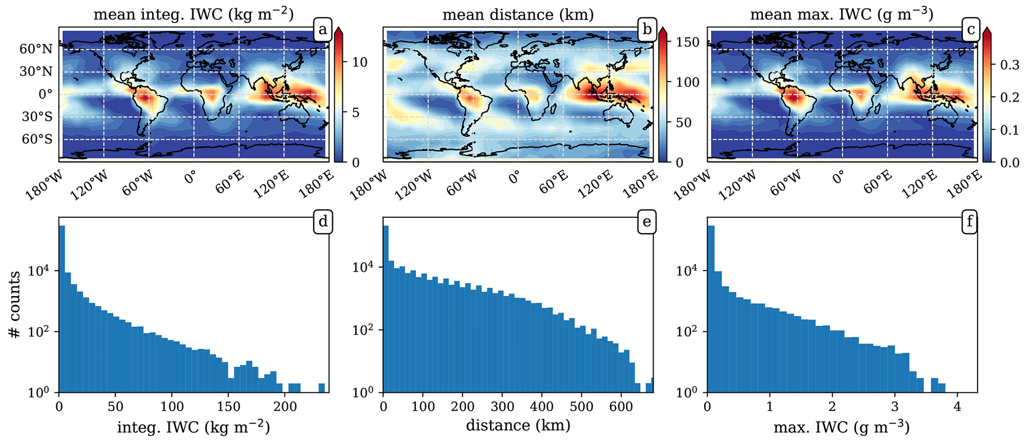
Figure 2Statistics of the CloudSat-RO database corresponding to the rays whose tangent height is 9 km. Panels (a–c) show the mean value climatology for the along-ray integrated IWC, distance (i.e., distance traveled by each ray within the influence of positive IWC), and maximum IWC encountered along the ray, respectively. The used grid is 10×10∘. Panels (d–f) correspond to the histograms for the total values for the same integrated IWC, distance, and maximum IWC, as in the first row. The IWC source is the DARDAR retrieval product.
The spatial/geographical patterns are also relevant. Higher concentrations of IWC at 9 km occur in the tropics (as expected), specially over land (South America and central Africa) and around the western Pacific Warm Pool. Regarding the distance, large values also appear over the mid- and high- latitude oceans. This results agree well with known patterns and the previous characterization of storm features, such as in Liu and Zipser (2015), meaning that the RO geometry does not pose a problem in obtaining these global properties of heavy precipitation systems. Therefore, this database of IWC in RO geometry is well suited to both help understand the features observed in the PAZ ΔΦ and relate them to realistic precipitating systems.
For this study, the DARDAR V3 retrieval has been used as a reference for the cross-comparison with ΔΦ. The choice has been made by taking into account the assumptions in the IWC retrieval of both DARDAR and 2B-CWC-RO. DARDAR V3 has been recently improved with in situ observations to help constrain the particle size distributions (Cazenave et al., 2019). A comparison between the integrated IWC from a CloudSat-RO generated from DARDAR V3 and 2B-CWC-RO products is shown in Fig. A1. The results shown hereafter will refer to those obtained using the CloudSat-RO generated from DARDAR V3.
As discussed in the introduction, both Kdp and WC are affected by the third moment of the N(D). Therefore, a relationship between the two is expected. Since the PRO observable (ΔΦ) is an integral measurement, the integrated IWC along the same ray where ΔΦ has been measured would be the most suitable quantity to be compared with. However, the PAZ satellite is in an 06:00/18:00 LT orbit optimized for its primary sensor, which results in few crossover measurements with the Global Precipitation Measurement (GPM) and CloudSat radars. Therefore, the comparison is performed statistically with the CloudSat-RO database.
For the ΔΦ observations, the whole PAZ mission is used. That is, 189 487 ΔΦ profiles between 10 May 2018 and 31 May 2022. All these profiles have been selected, so they have passed the initial quality controls and calibration (Padullés et al., 2020). PAZ ΔΦ data are available from https://paz.ice.csic.es/ (last access: 10 February 2023).
The noise of the individual ΔΦ observations is thoroughly assessed in Padullés et al. (2020). The noise is normally distributed around 0 mm (for the events with no clouds or precipitation), with a standard deviation that ranges from 1.5–2 mm in the lowest tangent heights (e.g., ∼2 km, where the signal-to-noise ratio of the observations is low) to 0.5 mm above 10 km. The major source of uncertainty for the IWC are the retrieval assumptions, and it has been briefly discussed in Appendix A.
Figure 3 shows the comparison of the mean along-ray-integrated IWC with the mean ΔΦ, as a function of latitude, corresponding to a tangent height of 7 km. It can be seen how the two quantities agree remarkably well when whole datasets are considered (Fig. 3a). The agreement is specially good over ocean (Fig. 3b). In the tropics, the shape of both the along-ray-integrated IWC and ΔΦ capture the global precipitation signature of the Intertropical Convergence Zone (ITCZ) very well (e.g., Marshall et al., 2014; Schneider et al., 2014). Over land (Fig. 3c), the agreement is also good, despite some small deviations between both quantities around the Equator.
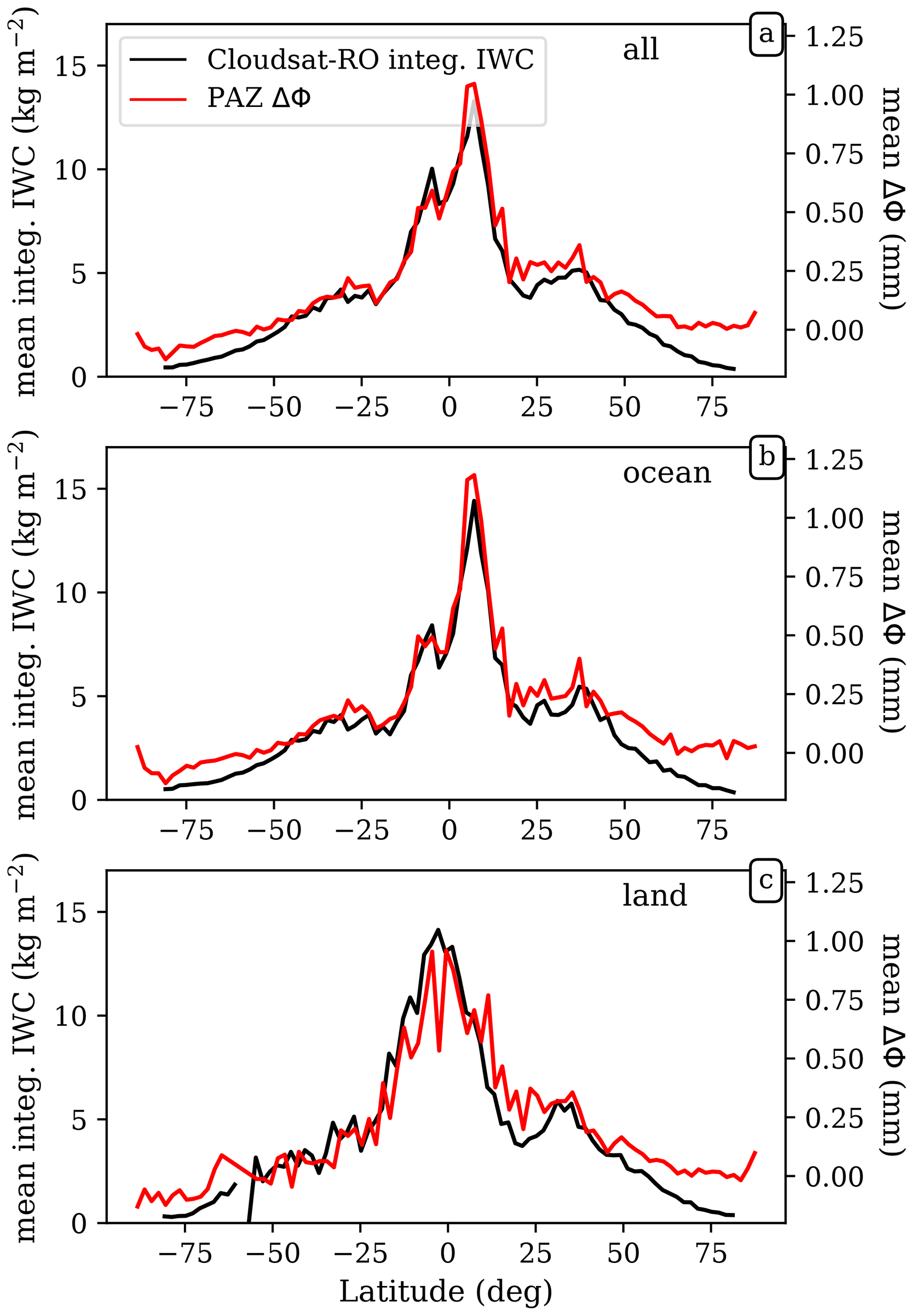
Figure 3Mean values of integrated IWC (left axes) from the CloudSat-RO dataset and mean values of observed ΔΦ from PAZ (right axes), as a function of latitude, for all data (a), over the ocean (b), and on land (c). Data correspond to tangent heights of 7 km. The mean values are computed for every 2∘ latitude bands.
On a map, the gridded mean (or climatology) of ΔΦ can be seen in Fig. 4. Figure 4a corresponds to the mean ΔΦ at a tangent height of 7 km and Fig. 4b at a tangent height of 9 km. The latter can be compared with Fig. 2a to investigate whether the spatial patterns are equivalent or not. In order to quantify the spatial relationship between the two (e.g., PAZ ΔΦ and CloudSat-RO IWC), the mean of both quantities is computed on the same grid. The chosen grid is 15×15∘, so that spatial patterns of precipitation arise, and there are enough PAZ observations to achieve significant statistics. The values for the mean of PAZ ΔΦ and integrated CloudSat-RO IWC obtained at the same grid cells are compared against each other (e.g., Fig. 5a). For the case of data corresponding to a tangent height of 9 km, the relationship follows a linear trend. The Pearson's correlation coefficient is 0.84 (e.g., r2=0.7), therefore exhibiting a robust relationship. The correlation coefficient for the spatial relationship between the mean PAZ ΔΦ and mean integrated CloudSat-RO IWC is computed for heights between 2 and 17 km.
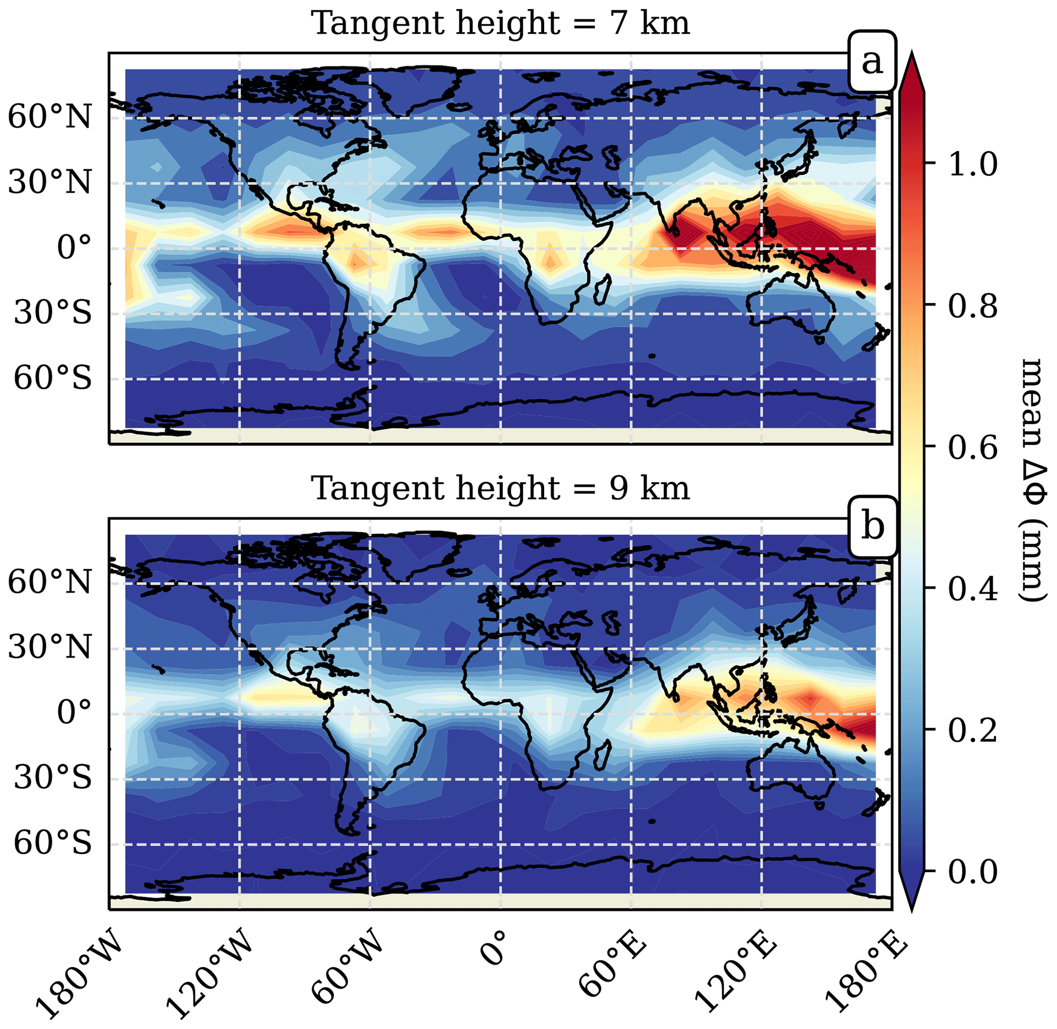
Figure 4Global climatology maps for the mean PAZ ΔΦ observations corresponding to a tangent height of 7 km (a) and 9 km (b). The grid size, where the means are computed, is 15×15∘.
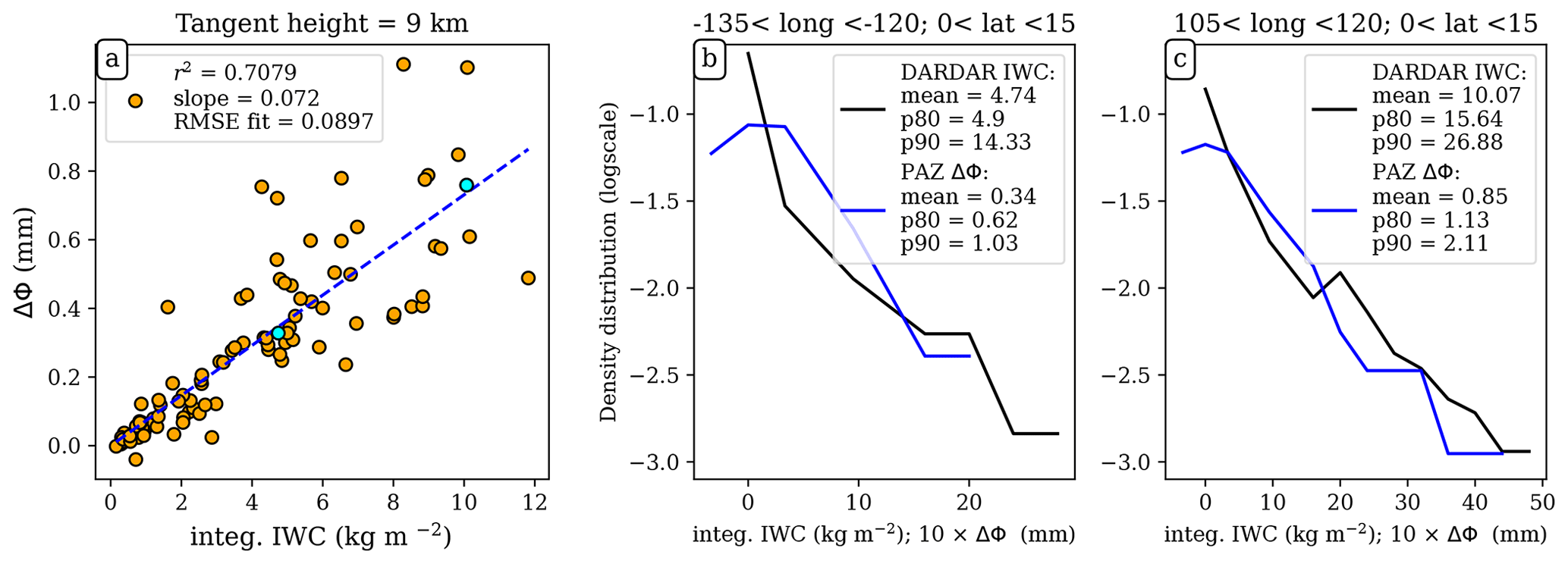
Figure 5Panel (a) shows the scatterplot of the mean climatologies of CloudSat-RO-integrated IWC vs. the PAZ ΔΦ obtained at the same grid cell, for the data corresponding to a tangent height of 9 km and over tropical ocean. Therefore, it is the comparison between the tropical ocean cells in Figs. 4b and 2a. Panels (b) and (c) show the distribution of CloudSat-RO-integrated IWC (black) and PAZ ΔΦ (blue) for two different grid cells at a tangent height of 9 km. The grid cells correspond to the two cyan points in panel (a), and its location is identified in the panel title, with the corresponding longitude and latitude ranges.
In addition to the mean, the 80th and 90th percentiles of both datasets are also computed at the same grid cells. That is, for each grid cell, the distribution for ΔΦ and for the CloudSat-RO-integrated IWC is represented, and the 80th and 90th percentiles of such distributions are computed. This results in a climatology for the 80th and 90th percentiles of ΔΦ and CloudSat-RO-integrated IWC. The approach is shown for two grid cells in Fig. 5b and c. The comparison between the 80th and 90th percentiles climatologies of ΔΦ and CloudSat-RO-integrated IWC is performed in order to check if the relationships stands at the higher ends of the distributions. That is, to check whether there is a good agreement between ΔΦ and integrated CloudSat-RO IWC for the whole distribution (and not only for the mean). The results are shown in Fig. 6.
Along with the correlation coefficient, the ratio between the PAZ ΔΦ mean climatology and the CloudSat-RO-integrated IWC mean climatology (i.e., ratio = ) is also computed at the same heights as the correlation coefficients and is shown in Fig. 7. It is computed from the linear fit between the mean PAZ ΔΦ and mean CloudSat-RO integrated IWC at different cells (e.g., see Fig. 5a, where we assume that the intercept is zero).
3.1 Correlations
The correlation coefficients in Fig. 6 quantify the agreement between the spatial or geographical patterns of the two datasets. High correlations can be understood as the two datasets observing the same kind of precipitation structures. One thing to note before digging deeper into the results is that the correlation coefficient is computed assuming a linear relationship between the two quantities.
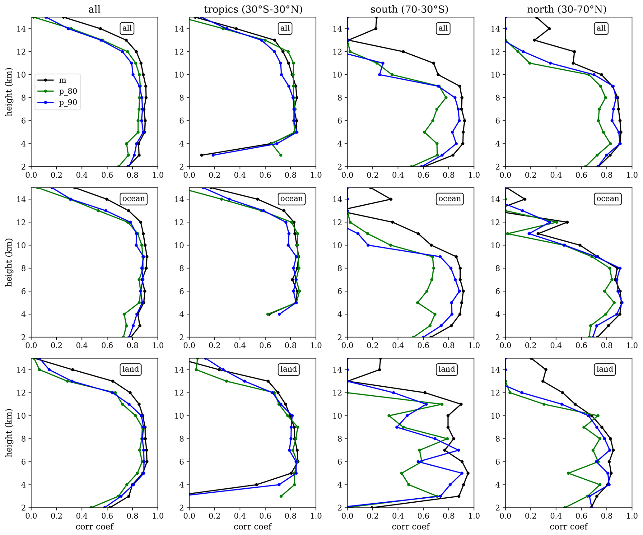
Figure 6Correlation coefficients between PAZ ΔΦ and CloudSat-RO IWC, as a function of height (y axis), for different areas across the globe (all globe, tropics, southern extratropics, and northern extratropics) and different surfaces (all, ocean, and land). The black lines correspond to the mean climatologies, the green lines to the 80th percentile, and the blue lines to the 90th percentile climatology.
The results, in general (e.g., Fig. 6 – first row), show a very high correlation coefficient (i.e., cc>0.8) among most of the considered heights. The correlation is particularly high over the oceans, although over land the agreement is also good. This is true for the three statistics being considered, i.e., the mean climatology and the climatologies for the 80th and 90th percentile of the distributions. However, the correlation coefficient corresponding to the mean tends to be slightly higher than the other two.
When the data are split in different regions (e.g., tropics vs. extratropics), then more detailed features can be explored. The first relevant one is the fact that the correlation coefficient in the tropics (Fig. 6 – second column) is higher for a wider range of heights than for the extratropical cases (Fig. 6 – third and fourth columns). Also, it can be seen how, for heights below ∼4 km, the correlation in the tropics drops due to the fact that the profiles have been truncated below the freezing level, and therefore, there are almost no data below ∼4 km. The second relevant feature is that the correlation for the climatologies of the 80th and 90th percentiles are lower outside the tropics. Finally, one must note that the panel corresponding to land in the Southern Hemisphere (70–30∘ S) is contributed by a relatively small number of data points, hence exhibiting a large dispersion of the correlation coefficients among different heights.
3.2 Ratios
The ratio between the mean climatologies of PAZ ΔΦ and CloudSat-RO-integrated IWC provides an empirical relationship between the two quantities, and it is shown in Fig. 7 (black line). Furthermore, the uncertainty of such a ratio (e.g., defined here as the root mean squared error around the linear fit) is obtained at each height when performing the linear regression between the mean climatologies (e.g., as shown in Fig. 5a).
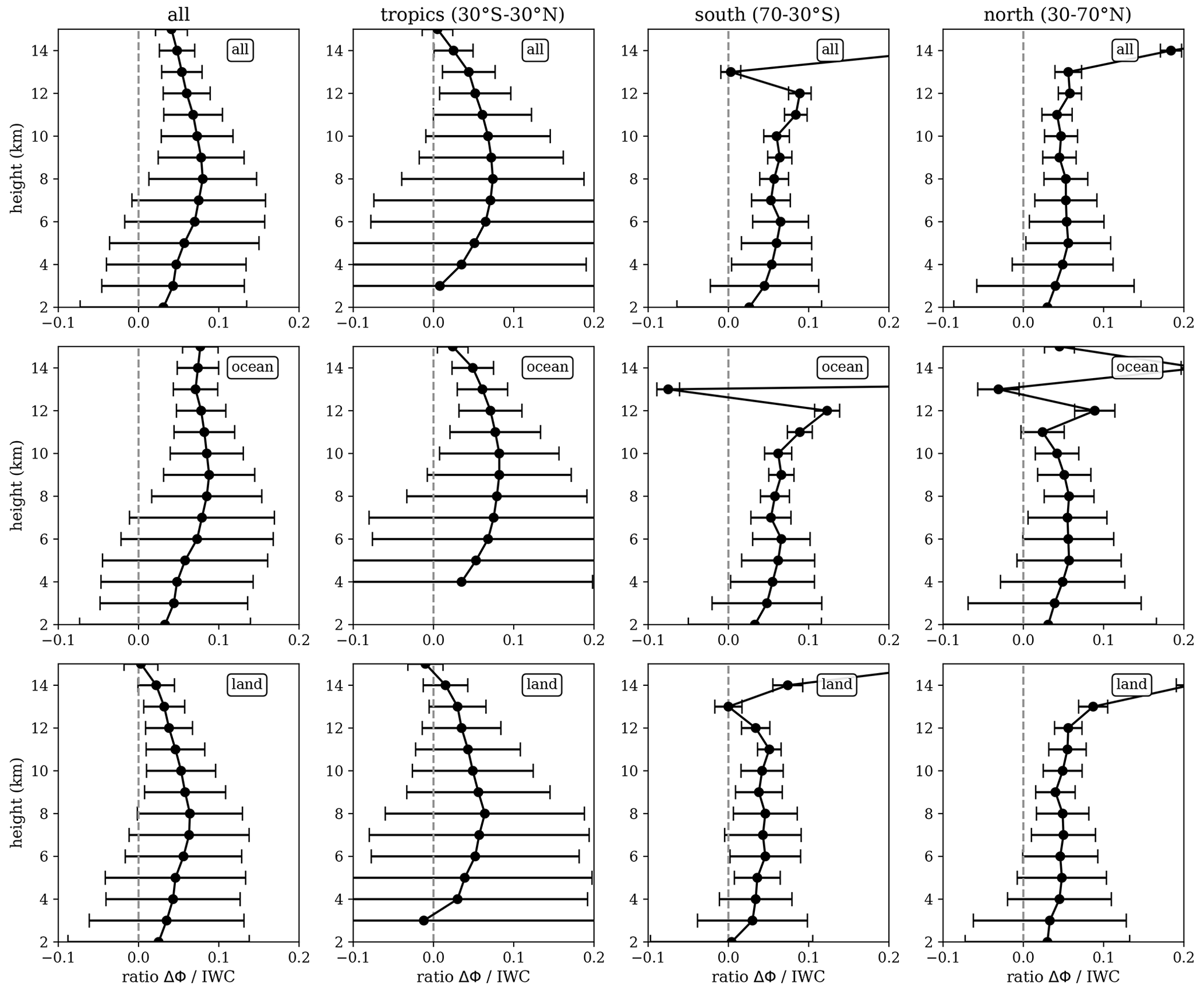
Figure 7Ratio between PAZ ΔΦ mean climatology and CloudSat-RO-integrated IWC mean climatology, as a function of height (y axis), for different areas across the globe (all globe, tropics, southern extratropics, and northern extratropics), and different surfaces (all, ocean, and land). The x axis error bars show the root mean squared error around the fit from which we obtain the ratio (e.g., see Fig. 5).
The ratio is considered meaningful in the heights and regions where the correlation coefficient is high (e.g., cc>0.8). The values obtained for the ratio of the mean climatologies in such regions and heights ranges from 0.03–0.09 mm kg−1 m2. It can be seen how it has a trend with height. In general, the ratio tends to maximize at around km in the tropics and at a lower heights in the extratropics.
The correlation coefficients obtained in Sect. 3.1 indicate a robust relationship between ΔΦ and integrated IWC, especially over tropical ocean. However, the meaning of the ratio between ΔΦ and integrated IWC depends on more factors. The aim of this section is to determine whether the ratios in Sect. 3.2 are physically meaningful or not. That is, to determine if the ratios are compatible with the characteristics of hydrometeors that are known to be present in clouds.
For this, the idea is to compute the Kdp–IWC relationship for a series of different hydrometeors and ice particle habits. This relationship can then be compared with the ratios in Fig. 7. To perform such comparison, first, the scattering amplitude matrix S is computed for a set of different single hydrometeors and ice particle habits. Then, a set of particle size distributions from 1 week of CloudSat observations are used to generate the corresponding Kdp and IWC using Eqs. (2) and (3). Note that, for this study, only single-particle scattering is considered.
4.1 Hydrometeors and ice particle habits
The forward-scattering simulations used for this study have been done using Rayleigh approximation. This formulation assumes that the particles can be approximated as oblate spheroids, with a certain axis ratio and effective density. The list of hydrometeors and ice particle habits that have been used are pristine ice crystals, aggregates of pristine ice, and wet snow. The adequacy of using Rayleigh approximations is justified by the long wavelength of GNSS signals, i.e., ∼190.3 mm, which is much larger than the typical size of frozen hydrometeors. For Rayleigh approximations, the formulations in Ryzhkov et al. (2011) and Bringi and Chandrasekar (2001) have been followed. That is, the forward-scattering amplitude co-polar components are computed using
where ϵ is the dielectric constant, and Lhh,vv are the shape parameters.
where ar is the axis ratio of the particle. For the dielectric constant, the Maxwell–Garnett formula is used in order to account for the effective density of the particles as mixtures of ice, air, and water (Maxwell Garnett, 1904). Below, there are the specific details for each of the hydrometeors and habits used in this study.
4.1.1 Pristine ice crystals
The simplest type of particles used in this study are pristine ice dendrites and thick plates. For the Rayleigh computation, the density of solid ice is used, and the values in Ryzhkov et al. (2011, Table 1) are used for the axis ratio. A fully horizontal orientation of the particles is assumed.
4.1.2 Aggregates
For more complex shapes, we use aggregates of pristine ice particles. For the Rayleigh approximation, a spheroid of air filled with portions of ice is used, following Ryzhkov et al. (2011) and taking different values for the effective density and axis ratio. The computation is performed for effective densities ranging from 0.1 to 0.9 g cm−3 and axis ratios ranging from 0.2 to 0.9. Note that using an effective density of 0.9 means that the spheroid is filled with ice, approaching a pristine ice particle. The results using the Rayleigh method for fixed densities and fixed-axis ratios for the whole range of equivalent diameters are called dry aggregates.
4.1.3 Wet snow
Finally, wet snow aims to represent frozen particles at the initial stages of melting. For this, the same spheroids as in the previous subsection are used, but for this case, a mass fraction of liquid water of a 10 % of the total mass is used, in addition to pure ice and air, to compute ϵ. The presence of water in the particle enhances ϵ, which in turn increases the Kdp with respect to the dry aggregates with same parameters (of equivalent density and ar).
4.2 Orientation angle distribution
The results for pristine ice, aggregates, and wet snow are computed using single-particle scattering and forcing the different particles to be horizontally oriented. This is unlikely to be the case in real clouds and storms, where the orientation of these particles is more complex. To account for different orientation angles, we assume a Gaussian distribution of tilt (or canting) angles centered at 0∘ (hence, the mean angle of β=0∘) with a certain standard deviation σ. This implies that, by varying σ, we can range from total horizontal orientation (σ=0∘) to completely random orientation (large σ). To keep the computations simple, we can use the horizontal orientation values and multiply them by a factor that accounts for such canting (Oguchi, 1983):
4.3 Simulations results
Using 1 week of CloudSat-retrieved N(D) at different heights above the freezing level, the IWC and Kdp are computed using the same particle type. This results in a set of Kdp vs. IWC relationships for different hydrometeors or ice particle habits and different properties such as effective density (ρ) and axis ratios. In addition, for each combination of particle type, ρ, and ar, the corresponding result at different distributions of tilt angles are performed. In Fig. 8, the variability in the Kdp vs. IWC relationship is shown, for dry aggregates (and wet snow), when one of the properties is varied (e.g., distribution of tilt angles – Fig. 8a; effective density – Fig. 8b; axis ratio – Fig. 8c; effective density for wet snow – Fig. 8d).
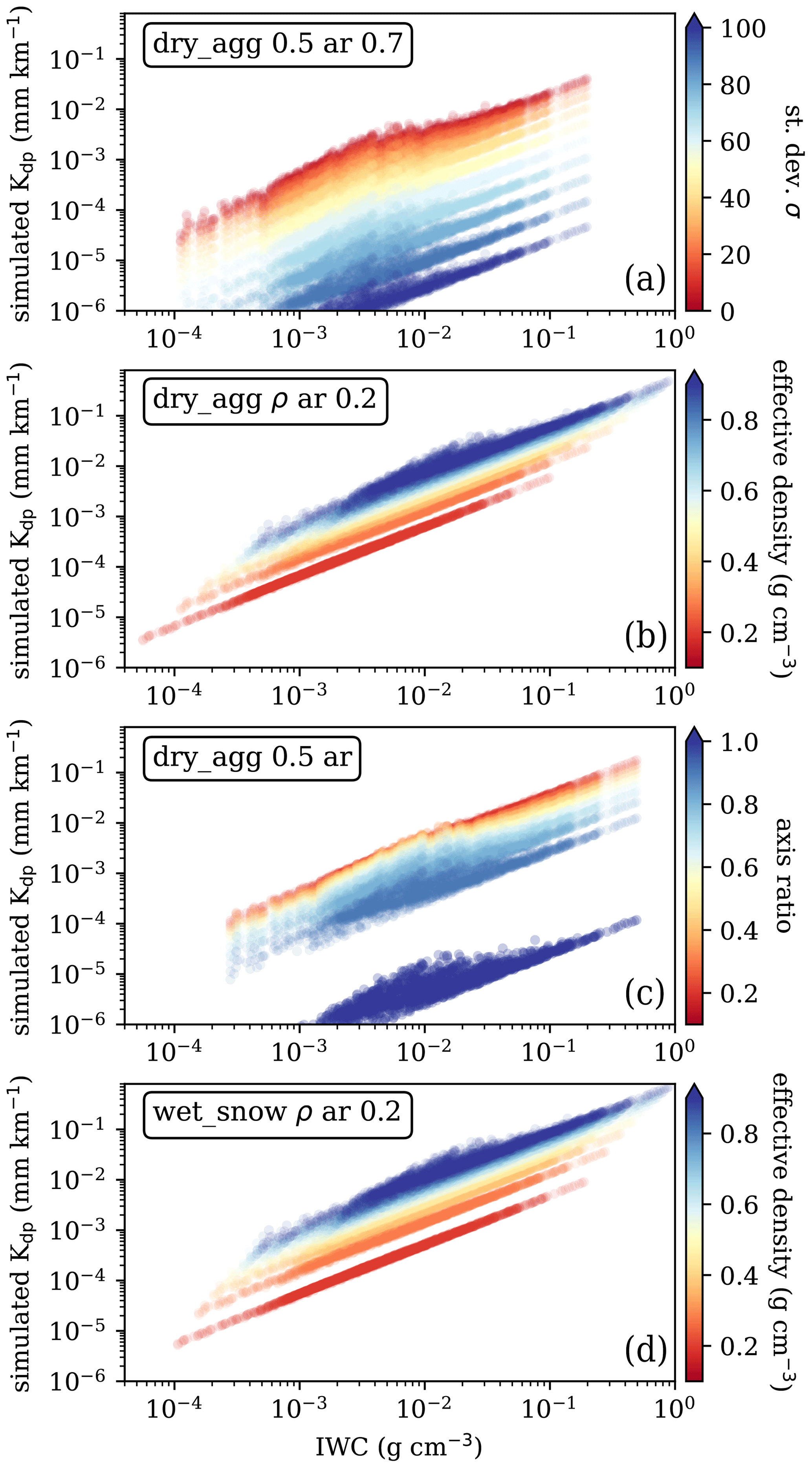
Figure 8Results of simulated Kdp as a function of IWC for dry aggregates (a–c) and wet snow (d), varying the standard deviation of the tilt angle distribution (a), the effective density (b), the axis ratio (c), and the effective density of wet snow (d).

Figure 9Results of the distributions of simulated ΔΦ vs. integrated IWC (a–c) and vs. the observed ΔΦ (d–f) compared at the same grid bins (same approach and same grid bins as in Fig. 4) and accounting for all heights. Panels (a) and (d) show the results obtained using a single type of particle at all locations and heights, where the dry aggregates have an effective density of 0.2 g cm−3 and an axis ratio of 0.7. Panels (b) and (e) correspond to results using dry aggregates with an effective density of 0.9 g cm−3 and an axis ratio of 0.2, and panels (c) and (f) correspond to results using dry aggregates with an effective density of 0.5 g cm−3 and an axis ratio of 0.5. The different colors of the contours correspond to a different standard deviation in the distribution of tilt angles, as described in the legend. The dashed contours (in panels a–c) correspond to the observed relationships (as obtained in Sect. 3). The dashed line (in panels d–f) indicates the perfect 1:1 agreement. The same color inner and outer contours represent the contour containing 30 % and 70 % of the data, respectively.
The ratios between the Kdp and IWC for a subset of particles and different properties are shown in Table 1. The ratios with a value within the range [0.03–0.09] are highlighted in bold. These are the values agreeing with the reported ratios between ΔΦ and integrated IWC in Sect. 3.
Table 1Ratio between Kdp and IWC for the different hydrometeors shown in Fig. 8 when a certain standard deviation is assumed in the orientation distribution (Gaussian distribution centered at 0∘ and σ), and σ=0∘ represents the scenario in which all particles are horizontally oriented, while for large σ, all particles would be randomly oriented (see Eq. 7). In bold, the ratios within the range [0.03–0.09] are shown, which is in agreement with the observed ratios in Fig. 6.
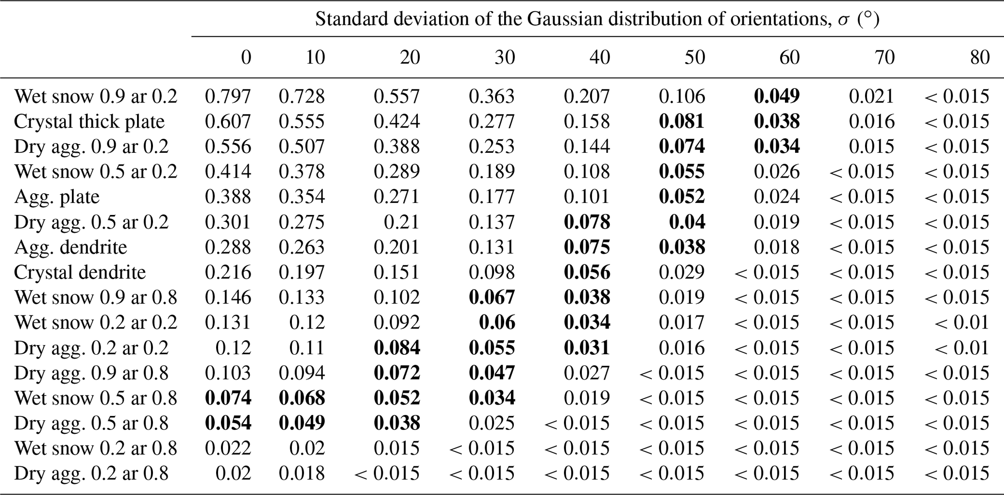
In these results, it can be seen how, for more pristine and thin particles, a certain canting angle is required (e.g., fully horizontal orientation is overestimating the observed Kdp), whereas, for more complex particles, these are required to stay more horizontally oriented to better match the actual data. It can also be observed that very low-density particles with high-axis ratios (i.e., approaching empty spheres) alone cannot explain the observations.
To further validate observations and results obtained in Sect. 3 and allow for a more equivalent comparison between the results, a simple exercise is performed. It consists of computing the integrated IWC and ΔΦ using the simulations just described and proceeding with the same procedure followed in Sect. 3 in order to obtain the same relationships, i.e., to compute the mean climatological values at the same grid bins and heights, but in this case, for the simulated ΔΦ values. The obtained values for ΔΦ at all grid bins and heights are shown as a function of the corresponding integrated IWC at the same grid bins and heights in Fig. 9 (top row). This is done for dry aggregates with a different combination of ρ and ar and for a different tilt angle distribution. The same approach is used to compare the simulated ΔΦ with the observed one, as shown in Fig. 9 (bottom row).
For simplicity, these results are obtained assuming the same hydrometeor type at all heights for all situations, which is unrealistic. Similarly, the same effective density has been assumed for each hydrometeor at different sizes, while a more realistic approach would be to assume that the density decreases with particle size. However, these simulations can be used to explain the bulk of the observations and further assess the effect of considering more or fewer tilted particles in the simulations in reproducing the observations. Comparing the simulated results with the observations (represented in the top row of Fig. 9 as a dashed black contour), it can be seen how the bulk observations can be reproduced using dry aggregated particles with a diversity of effective densities and axis ratios, depending on the tilt angle distribution. For example, dry aggregates with ρ=0.9 g cm−3 and ar=0.2 must have a standard deviation of the tilted angle distribution which is larger than 50∘ in order to explain the observed relationships.
5.1 Observations
The relationship between the PRO-observable ΔΦ and ice water content has been investigated in a global and statistical (or climatological) way. For this purpose, retrievals from the CloudSat mission have been used. These have been remapped into the RO observation geometry so that comparisons take into account the important features of the observation geometry of PRO. An important one is the long distances that rays traveling from the GNSS satellites to the receivers in the low Earth orbit spend in the lower layers of the troposphere. Such remapping allows an evaluation of the geometry itself. Thus, it can be assessed whether a limb-sounding measurement like PRO is able to capture important features of precipitation or not.
The results in Fig. 2 show the agreement between the climatology of the along-ray-integrated ice water content (and related products, such as the distance rays traveled within areas of non-zero ice water content or the maximum ice water content encountered per ray) with known and previously studied heavy precipitation features (e.g., Liu and Zipser, 2015). This is further confirmed with the results in Fig. 3 (showing the mean climatology as a function of latitude for water content; solid black line), which agrees very well with the signature of the ITCZ. Therefore, the good climatological agreement enables the use of the CloudSat-based artificially collocated RO database of along-ray-integrated ice water content for understanding the PRO observations of precipitating cloud structures. For this study, only ice water content retrievals are used, and the RO profiles are truncated at the freezing level. The use of ice-only retrievals is justified because CloudSat observations in the liquid region of deep-cloud structures (such as those specifically targeted by the ROHP experiment) may be degraded due to the high frequency and penetration issues.
The PRO-observable ΔΦ is the integrated Kdp along each RO ray. Both Kdp and water content are affected by the third moment of the N(D), and therefore, a relationship between them is to be expected. Such a relationship is investigated by evaluating the correlation coefficient between the geographical patterns of the high and low concentrations of ΔΦ and along-ray-integrated IWC, which is split in different regions and heights. Overall, correlation coefficients (e.g., Fig. 6) are high for the heights where frozen particles are expected (which changes by region; e.g., tropics vs. outside tropics). The correlation coefficients maximize for tropical oceans.
When the correlation coefficient is evaluated for the higher ends of the distribution (i.e., the climatologies for the 80th and 90th percentiles), then similar behavior is observed in the tropics, whereas differences between the mean climatology and the higher percentiles are observed in the mid-latitudes, especially over the southern oceans. This means that the features exhibited in the tail of the distribution of the retrieved IWC in this region are not well captured by PAZ ΔΦ. One hypothesized explanation could relate to the retrievals within mixed-phase clouds in the Southern Ocean (which are present in the lower heights in these areas) that have posed a long-standing issue for observations (e.g., Mace et al., 2021). Hence, further work must be carried out to assess whether the discrepancies between PAZ ΔΦ and CloudSat-retrieved ice water content in these areas are due to microphysical reasons (smaller ice particles, lack of preferred orientation, etc.), observational errors, or still unaccounted for factors.
The ratio between the mean climatology of ΔΦ and CloudSat-RO-integrated IWC aims at quantifying the empirical relationship between both. Results in Fig. 7 show the empirical relationship, along with its uncertainty, at each height and for different regions. The found ratio lies between 0.03 and 0.09 mm kg−1 m2. The uncertainties show the variation in the ratio around its mean, and it shows how, even for mean climatological values, there is a large dispersion that may be explained in part by the non-unique relationships between ΔΦ and integrated IWC.
This has in fact been observed in Gong and Wu (2017), where a decrease in the passive microwave polarimetric brightness temperature difference at 166 and 89 GHz is seen at very cold brightness temperatures associated with very deep convective areas. An extreme example of such a scenario applied here could be a region of large IWC with totally randomly oriented particles, where the ratio between ΔΦ and IWC would tend to 0, despite having high IWC. This effect would be masked in the mean climatology but could appear in individual observations. A more detailed study should be conducted to assess these situations, desirably with coincident observations between PRO and radars.
Another interesting feature of the ratio between ΔΦ and IWC shown in Fig. 7 is that it is, in general, not constant with height. This could be associated with the presence of different particles at different heights, consistent with particle shape dependence on temperature and supersaturation (e.g., Bailey and Hallett, 2009). Furthermore, differences in the ratio trend with height can be observed between over-ocean and over-land results, especially in the tropics, where a decrease in the correlation coefficient is observed at lower heights than for over the ocean. Two main hypothesis could explain the differences, i.e., (1) differences in the microphysics over ocean and over land impacting the shape and orientation of the frozen particles and (2) differences owing to different local time observations between PAZ (06:00/18:00 LT) and CloudSat (01:30/13:00 LT). The latter would have a stronger effect over land, but to discern between the two hypotheses, more observations at different orbital planes are needed.
The robust relationships between PRO ΔΦ and integrated IWC has an implicit and important implication; it demonstrates the systematic presence of horizontally oriented frozen particles thorough the different vertical cloud layers (above freezing level) globally. This conclusion expands upon results in Defer et al. (2014), Gong and Wu (2017), and Zeng et al. (2019), where the presence of horizontally oriented particles was observed globally using the Microwave Analysis and Detection of Rain and Atmospheric Structures (MADRAS) instrument on board the Megha-Tropiques satellite and the Global Precipitation Mission (GPM) Microwave Imager (GMI) polarization differences (PDs) at 157, 89, and 166 GHz. Thanks to the off-nadir-looking instrument, the PDs can be related to differential extinction by asymmetric particles. Also, similar to ΔΦ, using PDs from passive microwave radiometers provide a single-column measurement but in the quasi-vertical direction. Here, however, we can include the vertical information lacking in off-nadir-looking microwave measurements.
5.2 Simulations
Seeking to assess the feasibility of the results in Sect. 3, single-particle forward-scattering simulations have been used to assess whether the relationships obtained between ΔΦ and ice water content are reliable, according to the typical types of hydrometeors found in clouds. The assumptions made for the simulations are quite simple, e.g., mostly focused on dry aggregates with a range of ρ, ar, and tilt angle distributions.
Using a subset of N(D) and the simulated S, the relationship between IWC and Kdp is shown in Fig. 8, where a wide diversity of combinations of tilt angle distributions, effective densities, and axis ratios are computed. Many different combinations yield similar results in the relationship of Kdp vs. IWC, revealing the large number of degrees of freedom in ice particle forward-scattering simulations.
The results of the ratio between Kdp and IWC for a subset of particles with some combinations of ρ, ar, and tilt angle distributions are summarized in Table 1. These are also compared with the results in Sect. 3.2. The comparison allows us to corroborate that the observed ratios in the regions with high correlation coefficients can be explained with the simulations using simple approximations and could potentially help constraining the plausible distributions of ice crystals that can reproduce the ratios. For example, particles with large-axis ratios (e.g., approaching spheres) cannot reproduce the bulk of observed ratios between ΔΦ and IWC. Similarly, thin, solid ice particles would need to be oriented with a large dispersion in the tilt angle for the ratios to be consistent with observations.
Statistically comparing the simulated and observed ΔΦ and IWC relationship, repeating the approach followed in Sect. 3 but using the simulated Kdp (Fig. 9), a fairly good agreement is also reached with simple assumptions about the particles and changing of the tilt angle distributions. However, the dispersion in Fig. 9 (bottom row), when comparing simulated with observed gridded mean ΔΦ, is probably indicating that using the same particle assumptions for all regions and heights is not realistic. A better simulation exercise would be required, e.g., with numerical weather prediction model outputs with detailed information about the hydrometeor species, to further constrain the valid particle shapes and tilt angle distributions that better match the observations (similar to what is done in Brath et al., 2020). However, and despite the simplicity, the results obtained here seem compatible with those by Brath et al. (2020). They showed how previously observed relationships between passive microwave brightness temperatures and their polarization differences could be explained to account for tilted large, thin snow plates or less tilted, more complex, snow aggregates.
An important note to add is that the results presented here are valid for the chosen IWC retrieval algorithm (in this case, the DARDAR V3) and are therefore dependent on that choice. In particular, the DARDAR V3 algorithm assumes non-spherical ice particle shapes (Delanoë and Hogan, 2010; Cazenave et al., 2019) as opposed to the 2B-CWC-RO algorithm, which uses spherical solid ice particles (Austin et al., 2009). However, none of them explicitly takes into account the orientation of such particles. As can be seen in Appendix A, differences between IWC retrieved in the 2B-CWC-RO product and DARDAR can be large at some heights. This results (not shown) in differences in the computed correlation coefficients at lower heights (i.e., near the freezing level), where the results using DARDAR exhibit larger values for a wider range of heights for most regions. Some differences also appear in the values of the ratios, as can be deduced from Fig. A1b and c. As a consequence, the combination of ρ, ar, and tilt angle distributions that explain the observed ratios would change, but for most of the cases considered in this study (i.e., above the freezing level), they would remain within equivalent ranges.
This study assessed the global relationship between polarimetric radio-occultation-observable ΔΦ and ice water content retrieved by CloudSat. First of all, the integrated IWC retrievals from CloudSat have been remapped into the RO-like geometry. This has been used to demonstrate that RO-type limb-sounding observations can be used to sense and detect known precipitation features globally.
The global climatology of CloudSat-retrieved integrated IWC has been compared to the ΔΦ climatology from PAZ. It has been shown how the spatial/geographical correlation between the two datasets is high (cc>0.8) for a wide range of heights, including both ocean and land areas. This means that the IWC concentration patterns are well captured by PRO observations, both globally and at different heights. The correlation coefficient maximizes, and it is particularly good over tropical oceans for a range of heights ranging from 5 to 12 km.
The ratios between the mean ΔΦ and the mean integrated IWC climatologies are found to be within the range 0.03–0.09 mm kg−1 m2. Their analysis yields interesting results as well. First of all, the existence of such a relationship between both quantities implies the systematic presence of horizontally oriented hydrometeors contributing to IWC, both globally and at all heights. Second, the dispersion and differences at different heights indicate that different particles do indeed have a different ratio.
Furthermore, forward-scattering simulations of simple snow aggregates accounting for a range of effective densities, axis ratios, and tilt angle distributions can explain the bulk of the ratios (i.e., the mean climatological values). The simulation framework described here, although being very simple, can easily scale in complexity for arbitrary complex inputs of ice particle habits from, e.g., numerical weather prediction models or to account for more realistic assumptions about the effective density.
Despite the high correlation between the mean values of ΔΦ and integrated IWC, further work must be pursued to explore individual simultaneous observations of ΔΦ and IWC and assess when and under which scenarios the relationship holds (i.e., horizontally oriented particles contribute to the IWC) or does not apply (i.e., mostly non-oriented ice contributing to IWC). This is enabled by the fact that ΔΦ observations inherently provide unique information on the orientation of hydrometeors.
A comparison of the integrated IWC from the CloudSat retrieval using the 2B-CWC-RO and DARDAR V3 products has been performed and is shown in Fig. A1. The differences, in general, are shown in Fig. A1a. A more detailed view of the comparison between DARDAR V3 and 2B-CWC-RO-integrated IWC at different heights is shown in Fig. A1b, representing the fractional difference between the two datasets. The differences are positive (i.e., DARDAR V3 > 2B-CWC-RO) and larger at lower layers and shift to negative (i.e., DARDAR V3 < 2B-CWC-RO) at upper layers. A map showing how the differences are distributed in the grid cells used throughout the paper is given in Fig. A1c, for a tangent height of 6 km.
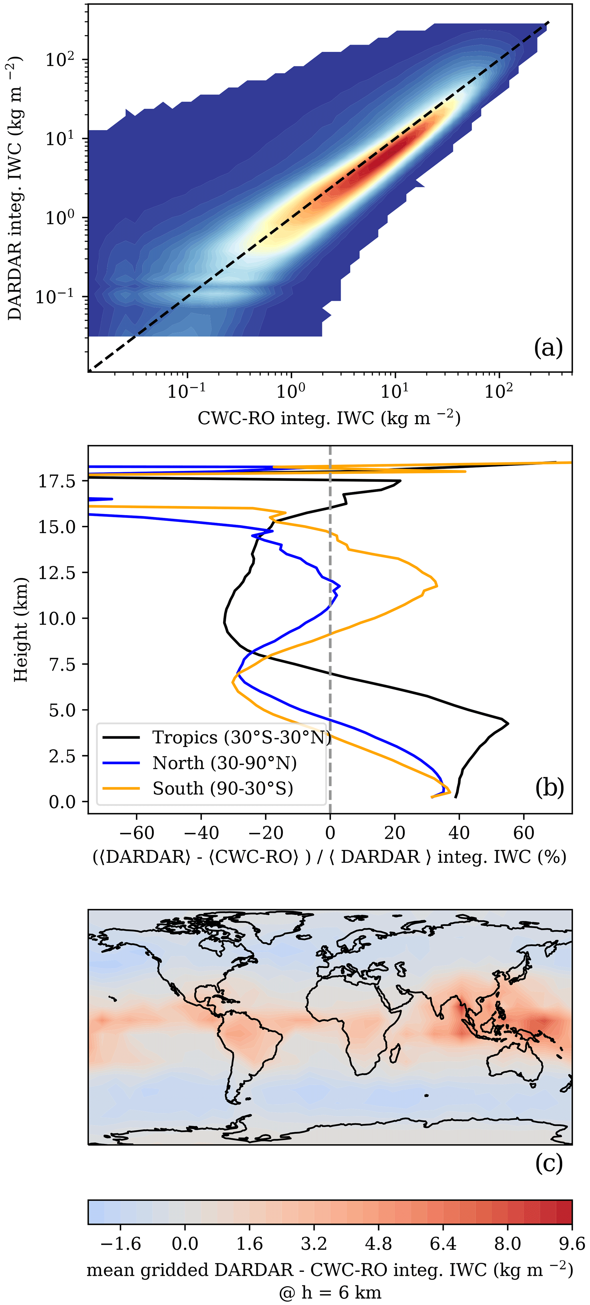
Figure A1Comparison between the integrated IWC from the CloudSat retrieval using the 2B-CWC-RO and DARDAR V3. Panel (a) shows the relationship between integrated IWC from the 2B-CWC-RO (x axis) and DARDAR V3 (y axis) for all observations, regardless of height. Panel (b) shows the fractional difference between the mean DARDAR V3 and 2B-CWC-RO-integrated IWC as a function of height, for three different latitudinal bands (see the legend). Panel (c) shows the gridded mean DARDAR–2B-CWC-RO-integrated IWC corresponding to a tangent height of 6 km.
The differences arise from different assumptions regarding the treatment of the CloudSat observations near the freezing level and the assumptions about the particle size distributions, and DARDAR includes Cloud-Aerosol Lidar and Infrared Pathfinder Satellite Observation (CALIPSO) observations to complement CloudSat observations (Delanoë and Hogan, 2008, 2010; Austin et al., 2009; Cazenave et al., 2019).
The differences in the integrated IWC would change the results from Sect. 3. The correlation coefficient exhibits lower values for heights near the freezing level when 2B-CWC-RO is used, and regions over land also exhibit a lower correlation coefficient with 2B-CWC-RO. The ratios between the ΔΦ and the integrated IWC change according to the differences between the two IWC products, since ΔΦ would be the same (e.g., see Fig. A1b).
The datasets used for this work are the PAZ polarimetric radio occultation data, which can be obtained from https://paz.ice.csic.es (ICE-CSIC/IEEC, 2023). The DARDAR dataset can be obtained from https://www.icare.univ-lille.fr/ (ICARE, 2023). The CloudSat 2B-CWC-RO dataset can be obtained from https://www.cloudsat.cira.colostate.edu/data-products/2b-cwc-ro (NASA, 2023).
All co-authors have reviewed, discussed, and agreed to the final version of the paper. RP, EC, and FJT conceptualized the paper. RP analyzed the data and prepared the original draft. The investigation was led by RP, EC, and FJT. RP reviewed and edited the paper with EC and FJT, who also acquired the funding.
The contact author has declared that none of the authors has any competing interests.
Publisher's note: Copernicus Publications remains neutral with regard to jurisdictional claims in published maps and institutional affiliations.
The authors would like to thank Patrick Eriksson and one anonymous reviewer, for their comments and suggestions, which definitely helped to improve the paper.
Ramon Padullés has received funding from the postdoctoral fellowship program, Beatriu de Pinós, funded by the Secretary of Universities and Research (Government of Catalonia) and by the Horizon 2020 Research and Innovation program of the European Union under the Marie Skłodowska-Curie Actions. The ROHP-PAZ project is funded by the Spanish Ministry of Science and Innovation and by the European Regional Development Fund (ERDF), as part of “A way of making Europe” for the European Union. Part of the investigations has been done under the EUMETSAT ROM SAF CDOP4 and is based upon work from CSIC-PTI TELEDETECT members. F. Joseph Turk acknowledges support from NASA under the U.S. Participating Investigator (USPI) program. The work performed by F. Joseph Turk has been conducted at the Jet Propulsion Laboratory, California Institute of Technology, under contract with NASA.
This research has been supported by the Agència de Gestió d'Ajuts Universitaris i de Recerca (grant no. 2019 BP 00110), the H2020 Marie Skłodowska-Curie Actions (grant no. 801370), and the Agencia Estatal de Investigación (grant nos. RTI2018-099008-B-C22, PID2021-126436OB, and MCIN/AEI/10.13039/501100011033). This work has also been partially supported by the program Unidad de Excelencia María de Maeztu (grant no. CEX2020-001058-M).
We acknowledge support of the publication fee by the CSIC Open Access Publication Support Initiative through its Unit of Information Resources for Research (URICI).
This paper was edited by Thijs Heus and reviewed by Patrick Eriksson and one anonymous referee.
Austin, R. T., Heymsfield, A. J., and Stephens, G. L.: Retrieval of ice cloud microphysical parameters using the CloudSat millimeter-wave radar and temperature, J. Geophys. Res.-Atmos., 114, 1–19, https://doi.org/10.1029/2008JD010049, 2009. a, b, c
Bailey, M. and Hallett, J.: A Comprehensive Habit Diagram for Atmospheric Ice Crystals: Confirmation from the Laboratory, AIRS II, and Other Field Studies, J. Atmos. Sci., 66, 2888–2899, https://doi.org/10.1175/2009JAS2883.1, 2009. a
Barlakas, V., Geer, A. J., and Eriksson, P.: Introducing hydrometeor orientation into all-sky microwave and submillimeter assimilation, Atmos. Meas. Tech., 14, 3427–3447, https://doi.org/10.5194/amt-14-3427-2021, 2021. a
Battaglia, A., Ajewole, M. O., and Simmer, C.: Evaluation of radar multiple scattering effects in Cloudsat configuration, Atmos. Chem. Phys., 7, 1719–1730, https://doi.org/10.5194/acp-7-1719-2007, 2007. a
Brath, M., Ekelund, R., Eriksson, P., Lemke, O., and Buehler, S. A.: Microwave and submillimeter wave scattering of oriented ice particles, Atmos. Meas. Tech., 13, 2309–2333, https://doi.org/10.5194/amt-13-2309-2020, 2020. a, b
Bringi, V. N. and Chandrasekar, V.: Polarimetric doppler weather radar: principles and applications, Cambridge University Press, Cambridge, ISBN 0-521-62384-7, 2001. a, b
Bukovčić, P., Ryzhkov, A. V., Zrnić, D. S., and Zhang, G.: Polarimetric radar relations for quantification of snow based on disdrometer data, J. Appl. Meteorol. Clim., 57, 103–120, https://doi.org/10.1175/JAMC-D-17-0090.1, 2018. a
Cardellach, E., Tomás, S., Oliveras, S., Padullés, R., Rius, A., de la Torre-Juárez, M., Turk, F. J., Ao, C. O., Kursinski, E. R., Schreiner, W. S., Ector, D., and Cucurull, L.: Sensitivity of PAZ LEO Polarimetric GNSS Radio-Occultation Experiment to Precipitation Events, IEEE T. Geosci. Remote, 53, 190–206, https://doi.org/10.1109/TGRS.2014.2320309, 2014. a, b
Cardellach, E., Oliveras, S., Rius, A., Tomás, S., Ao, C. O., Franklin, G. W., Iijima, B. A., Kuang, D., Meehan, T. K., Padullés, R., de la Torre-Juárez, M., Turk, F. J., Hunt, D. C., Schreiner, W. S., Sokolovskiy, S. V., Van Hove, T., Weiss, J. P., Yoon, Y., Zeng, Z., Clapp, J., Xia-Serafino, W., and Cerezo, F.: Sensing heavy precipitation with GNSS polarimetric radio occultations, Geophys. Res. Lett., 46, 1024–1031, https://doi.org/10.1029/2018GL080412, 2019. a
Cazenave, Q., Ceccaldi, M., Delanoë, J., Pelon, J., Groß, S., and Heymsfield, A. J.: Evolution of DARDAR-CLOUD ice cloud retrievals: New parameters and impacts on the retrieved microphysical properties, Atmos. Meas. Tech., 12, 2819–2835, https://doi.org/10.5194/amt-12-2819-2019, 2019. a, b, c, d
Davis, C. P., Wu, D. L., Emde, C., Jiang, J. H., Cofield, R. E., and Harwood, R. S.: Cirrus induced polarization in 122 GHz aura Microwave Limb Sounder radiances, Geophys. Res. Lett., 32, 1–4, https://doi.org/10.1029/2005GL022681, 2005. a
Defer, E., Galligani, V. S., Prigent, C., and Jimenez, C.: First observations of polarized scattering over ice clouds at close-to-millimeter wavelengths (157 GHz) with MADRAS on board the Megha-Tropiques mission, J. Geophys. Res.-Atmos., 119, 12301–12316, https://doi.org/10.1002/2014JD022353, 2014. a
Delanoë, J. and Hogan, R. J.: A variational scheme for retrieving ice cloud properties from combined radar, lidar, and infrared radiometer, J. Geophys. Res.-Atmos., 113, 1–21, https://doi.org/10.1029/2007JD009000, 2008. a
Delanoë, J. and Hogan, R. J.: Combined CloudSat-CALIPSO-MODIS retrievals of the properties of ice clouds, J. Geophys. Res., 115, D00H29, https://doi.org/10.1029/2009JD012346, 2010. a, b, c
Gong, J. and Wu, D. L.: Microphysical properties of frozen particles inferred from Global Precipitation Measurement (GPM) Microwave Imager (GMI) polarimetric measurements, Atmos. Chem. Phys., 17, 2741–2757, https://doi.org/10.5194/acp-17-2741-2017, 2017. a, b
Gong, J., Zeng, X., Wu, D. L., Munchak, S. J., Li, X., Kneifel, S., Liao, L., and Barahona, D.: Linkage among Ice Crystal Microphysics, Mesoscale Dynamics and Cloud and Precipitation Structures Revealed by Collocated Microwave Radiometer and Multi-frequency Radar Observations, Atmos. Chem. Phys., 20, 12633–12653, https://doi.org/10.5194/acp-20-12633-2020, 2020. a
Hajj, G. A., Kursinski, E. R., Romans, L. J., Bertiger, W. I., and Leroy, S. S.: A Technical Description of Atmospheric Sounding By Gps occultation, J. Atmos. Sol.-Terr. Phy., 64, 451–469, https://doi.org/10.1016/S1364-6826(01)00114-6, 2002. a
ICARE: CloudSat DARDAR-CLOUD product, https://www.icare.univ-lille.fr/, last access: 10 February 2023. a
ICE-CSIC/IEEC: ROHP-PAZ dataset, https://paz.ice.csic.es, last access: 10 February 2023. a
Jameson, A. R.: Microphysical Interpretation of Multiparameter Radar Measurements in Rain. Part III: Interpretation and Measurement of Propagation Differential Phase Shift between Orthogonal Linear Polarizations, J. Atmos. Sci., 42, 607–614, https://doi.org/10.1175/1520-0469(1985)042<0607:MIOMRM>2.0.CO;2, 1985. a
Kaur, I., Eriksson, P., Barlakas, V., Pfreundschuh, S., and Fox, S.: Fast Radiative Transfer Approximating Ice Hydrometeor Orientation and Its Implication on IWP Retrievals, Remote Sens. 14, 1–33, https://doi.org/10.3390/rs14071594, 2022. a
Kursinski, E. R., Hajj, G. A., Schofield, J. T., Linfield, R. P., and Hardy, K. R.: Observing Earth's atmosphere with radio occultation measurements using the Global Positioning System, J. Geophys. Res., 102, 23429–23465, https://doi.org/10.1029/97JD01569, 1997. a, b
Liu, C. and Zipser, E. J.: The global distribution of largest, deepest, and most intense precipitation systems, Geophys. Res. Lett., 42, 3591–3595, https://doi.org/10.1002/2015GL063776, 2015. a, b
Mace, G. G., Protat, A., and Benson, S.: Mixed-Phase Clouds Over the Southern Ocean as Observed From Satellite and Surface Based Lidar and Radar, J. Geophys. Res.-Atmos., 126, e2021JD034569, https://doi.org/10.1029/2021JD034569, 2021. a
Marchand, R., Mace, G. G., Ackerman, T., and Stephens, G. L.: Hydrometeor detection using Cloudsat - An earth-orbiting 94-GHz cloud radar, J. Atmos. Ocean. Tech., 25, 519–533, https://doi.org/10.1175/2007JTECHA1006.1, 2008. a
Marshall, J., Donohoe, A., Ferreira, D., and McGee, D.: The ocean's role in setting the mean position of the Inter-Tropical Convergence Zone, Clim. Dynam., 42, 1967–1979, https://doi.org/10.1007/s00382-013-1767-z, 2014. a
Maxwell Garnett, J. C.: Colours in Metal Glasses and in Metallic Films, Philos. T. Roy. Soc. Lond., 203, 385–420, https://doi.org/10.1098/rsta.1904.0024, 1904. a
NASA: CloudSat 2B-CWC-RO product, https://www.cloudsat.cira.colostate.edu/data-products/2b-cwc-ro, last access: 10 February 2023. a
Nguyen, C. M., Wolde, M., and Korolev, A. V.: Determination of Ice Water Content (IWC) in tropical convective clouds from X-band dual-polarization airborne radar, Atmos. Meas. Tech., 12, 5897–5911, https://doi.org/10.5194/amt-12-5897-2019, 2019. a
Oguchi, T.: Electromagnetic wave propagation and scattering in rain and other hydrometeors, Proc. IEEE, 71, 1029–1078, https://doi.org/10.1109/PROC.1983.12724, 1983. a
Padullés, R., Ao, C. O., Turk, F. J., de la Torre-Juárez, M., Iijima, B. A., Wang, K. N., and Cardellach, E.: Calibration and Validation of the Polarimetric Radio Occultation and Heavy Precipitation experiment Aboard the PAZ Satellite, Atmos. Meas. Tech., 13, 1299–1313, https://doi.org/10.5194/amt-13-1299-2020, 2020. a, b
Padullés, R., Cardellach, E., Turk, F. J., Ao, C. O., de la Torre-Juárez, M., Gong, J., and Wu, D. L.: Sensing Horizontally Oriented Frozen Particles With Polarimetric Radio Occultations Aboard PAZ: Validation Using GMI Coincident Observations and Cloudsat aPriori Information, IEEE T. Geosci. Remote, 60, 1–13, https://doi.org/10.1109/TGRS.2021.3065119, 2022. a, b
Ryzhkov, A. V., Zrnić, D. S., and Gordon, B. A.: Polarimetric method for ice water content determination, J. Appl. Meteorol., 37, 125–134, https://doi.org/10.1175/1520-0450(1998)037<0125:PMFIWC>2.0.CO;2, 1998. a
Ryzhkov, A. V., Pinsky, M., Pokrovsky, A., and Khain, A. P.: Polarimetric radar observation operator for a cloud model with spectral microphysics, J. Appl. Meteorol. Clim., 50, 873–894, https://doi.org/10.1175/2010JAMC2363.1, 2011. a, b, c
Schneider, T. L., Bischoff, T., and Haug, G. H.: Migrations and dynamics of the intertropical convergence zone, Nature, 513, 45–53, https://doi.org/10.1038/nature13636, 2014. a
Stephens, G. L., Vane, D. G., Tanelli, S., Im, E., Durden, S. L., Rokey, M., Reinke, D., Partain, P., Mace, G. G., Austin, R. T., L'Ecuyer, T., Haynes, J., Lebsock, M., Suzuki, K., Waliser, D. E., Wu, D. L., Kay, J., Gettelman, A., Wang, Z., and Marchand, R.: CloudSat mission: Performance and early science after the first year of operation, J. Geophys. Res.-Atmos., 113, 1–18, https://doi.org/10.1029/2008JD009982, 2008. a
Turk, F. J., Padullés, R., Cardellach, E., Ao, C. O., Wang, K.-N., Morabito, D. D., de la Torre-Juárez, M., Oyola, M., Hristova-Veleva, S. M., and Neelin, J. D.: Interpretation of the Precipitation Structure Contained in Polarimetric Radio Occultation Profiles Using Passive Microwave Satellite Observations, J. Atmos. Ocean. Tech., 38, 1727–1745, https://doi.org/10.1175/jtech-d-21-0044.1, 2021. a
Vivekanandan, J., Bringi, V. N., Hagen, M., and Meischner, P.: Polarimetric radar studies of atmospheric ice particles, IEEE T. Geosci. Remote, 32, 1–10, https://doi.org/10.1109/36.285183, 1994. a
Wu, D. L., Austin, R. T., Deng, M., Durden, S. L., Heymsfield, A. J., Jiang, J. H., Lambert, A., Li, J. L., Livesey, N. J., McFarquhar, G. M., Pittman, J. V., Stephens, G. L., Tanelli, S., Vane, D. G., and Waliser, D. E.: Comparisons of global cloud ice from MLS, CloudSat, and correlative data sets, J. Geophys. Res.-Atmos., 114, 1–20, https://doi.org/10.1029/2008JD009946, 2009. a
Zeng, X., Skofronick-Jackson, G., Tian, L., Emory, A. E., Olson, W. S., and Kroodsma, R. A.: Analysis of the global microwave polarization data of clouds, J. Climate, 32, 3–13, https://doi.org/10.1175/JCLI-D-18-0293.1, 2019. a
- Abstract
- Introduction
- CloudSat retrievals projected to RO geometries
- Relationship between PAZ ΔΦ and CloudSat ice water content
- Forward-scattering simulations of ice and snow
- Summary and discussion
- Conclusions
- Appendix A: Comparison between DARDAR and 2B-CWC-RO integrated IWC profiles
- Data availability
- Author contributions
- Competing interests
- Disclaimer
- Acknowledgements
- Financial support
- Review statement
- References