Impact of formulations of the homogeneous nucleation rate on ice nucleation events in cirrus

Homogeneous freezing of solution droplets is an important pathway of ice formation in the tropopause region. The nucleation rate can be parameterized as a function of water activity, based on empirical fits and some assumptions on the underlying properties of super-cooled water, although a general theory is missing. It is not clear how nucleation events are influenced by the exact formulation of the nucleation rate or even their inherent uncertainty. In this study we investigate the formulation of the nucleation rate of homogeneous freezing of solution droplets (1) to link the formulation to the nucleation rate of pure water droplets, (2) to derive a robust and simple formulation of the nucleation rate, and (3) to determine the impact of variations in the formulation on nucleation events. The nucleation rate can be adjusted, and the formulation can be simplified to a threshold description. We use a state-of-the-art bulk ice microphysics model to investigate nucleation events as driven by constant cooling rates; the key variables are the final ice crystal number concentration and the maximum supersaturation during the event. The nucleation events are sensitive to the slope of the nucleation rate but only weakly affected by changes in its absolute value. This leads to the conclusion that details of the nucleation rate are less important for simulating ice nucleation in bulk models as long as the main feature of the nucleation rate (i.e. its slope) is represented sufficiently well. The weak sensitivity of the absolute values to the nucleation rate suggests that the amount of available solution droplets also does not crucially affect nucleation events. The use of only one distinct nucleation threshold function for analysis and model parameterization should be reinvestigated, since it corresponds to a very high nucleation rate value, which is not reached in many nucleation events with low vertical updrafts. In contrast, the maximum supersaturation and thus the nucleation thresholds reached during an ice nucleation event depend on the vertical updraft velocity or cooling rate. This feature might explain some high supersaturation values during nucleation events in cloud chambers and suggests a reformulation of ice nucleation schemes used in coarse models based on a purely temperature-dependent nucleation threshold.

1 Introduction

Clouds are one of the most important components in the Earth–atmosphere system. They influence the hydrological cycle and Earth's energy balance via interaction with radiation. Clouds can cool the system by partly scattering and reflecting incoming solar radiation (albedo effect) but also warm the atmosphere by absorbing and re-emitting thermal radiation as emitted by the Earth's surface (greenhouse effect). While for liquid clouds a net cooling effect can be derived, the radiative effect for clouds containing ice crystals is still under debate. In particular, for pure ice clouds (so-called cirrus clouds) at high altitudes in the low temperature range (T<235 K), the albedo effect and greenhouse effect are of the same order of magnitude but have different signs, leading to different net effects (see, for example, Fusina et al., 2007; Joos et al., 2014; Gasparini et al., 2017). Thus, details in microphysical properties of ice crystals might decide about a net warming or cooling of cirrus clouds, as can be seen in former model studies (e.g. Zhang et al., 1999). A key aspect of ice crystals is their size which directly affects the scattering and absorption of radiation. Smaller crystals scatter incoming solar light more effectively; thus the optical depth τ is directly dependent on the size, as can be seen in the usual approximation (see, for example, Fu and Liou, 1993)

$$\begin{array}{}\text{(1)}& \mathit{\tau }=\mathrm{IWC}\cdot \mathrm{\Delta }z\cdot \left(a+{\displaystyle \frac{b}{D_{\mathrm{e}}}}\right),\end{array}$$

where D_e denotes the effective diameter of the crystal, IWC is the ice water content, Δz represents the vertical extent of the cloud, and a and b are empirically derived constants. Since the available water vapour is mainly determined by thermodynamic conditions, the pathway of ice nucleation often determines the ice crystal number concentration in cirrus clouds and thus their effective size (assuming a certain amount of available water vapour).

Ice crystals can be formed by very different nucleation processes, which can be grouped into two major pathways, namely in situ and liquid origin ice formation (e.g. Krämer et al., 2016; Luebke et al., 2016; Wernli et al., 2016). The overall term “in situ formation” refers to ice formation at humidities below water saturation, whereas “liquid origin formation” subsumes all formation processes where cloud droplets are present and humidity is close to water saturation (e.g. freezing of cloud droplets); see the definition in Wernli et al. (2016). It is well known that the ice crystal number concentration varies crucially as a function of the underlying nucleation process, leading to potentially strong changes in the resulting radiative effect (see, for example, Krämer et al., 2020).

Despite the availability of many observational data and laboratory experiments (e.g. Hoose and Möhler, 2012), and also the development of new theoretical models (e.g. the soccer ball model; see Niedermeier et al., 2011), the details of ice nucleation at the molecular scale are still unknown.

A special situation occurs for the so-called homogeneous freezing of super-cooled solution droplets (also short: homogeneous nucleation) at cold temperatures below 235 K. This process describes the spontaneous freezing of super-cooled aqueous solution particles containing a small amount of (usually inorganic) substances. Although the details of this freezing process are also not completely understood on a molecular scale, reproducible laboratory experiments allowed for the formulation of an empirical fit for the nucleation rate (Koop et al., 2000). Such a fit bears inherent but maybe also unknown uncertainty, since we have no generally accepted theory for comparison. Other fits or a change in the fit parameters might also lead to different formulations of nucleation rates.

A priori, it is not clear how large the impact of the formulation of nucleation rates might be on simulating nucleation events in models resolving nucleation events in time. This issue is the starting point of our investigation. We want to address three different aspects. First, we want to link the former formulation by Koop et al. (2000) to recent findings on pure water in order to formulate a consistent framework for our models. Second, we want to derive a robust and simple formulation of the homogeneous nucleation rates, which can be used for analytical as well as numerical investigations. Third, we want to investigate the impact of variations of nucleation rates (based on the new formulation) on nucleation events, i.e. on the resulting ice crystal number concentrations.

From theory (e.g. Baumgartner and Spichtinger, 2019) and former idealized box model simulations (e.g. Kärcher and Lohmann, 2002; Ren and Mackenzie, 2005; Spichtinger and Gierens, 2009), we know that ice crystal numbers as produced in homogeneous nucleation events driven by a constant cooling rate (equivalent to a constant vertical velocity) crucially depend on several parameters and, thus, also affect the radiative properties of the formed ice cloud (see, for example, calculations in Krämer et al., 2020; Joos et al., 2009). Therefore, it is of high importance to understand the impact of the formulation of nucleation rates on the resulting ice crystal number concentrations.

We emphasize that all our investigations are meant in a bulk sense; i.e. only integrated quantities such as the ice crystal number and (total) ice crystal mass are considered. Using this approach, we consider the case of a newly forming cirrus cloud and do not focus on the freezing or forming details of single ice crystals.

The study is structured as follows. In the next section, we present the fit by Koop et al. (2000) and its empirical basis, as related to water theories. In Sect. 3 we describe the simple model used for idealized simulations for testing the impact of different formulations of nucleation rates. In Sect. 4 the more compact formulation of the nucleation rate along with several approximations is discussed. The consequences of using the proposed approximations are explored by idealized numerical simulations. In Sect. 5 we investigate the impact of a recently proposed formulation of the saturation vapour pressure over super-cooled liquid water on the nucleation events (Nachbar et al., 2019). In Sect. 6 a new formulation of the nucleation rate based on results for freezing of pure super-cooled water (Koop and Murray, 2016) is presented, and its impact on the number concentration of nucleated ice crystals is discussed. In Sect. 7 we investigate thresholds of ice nucleation as well as the peak values of supersaturation during nucleation events, Finally, we summarize the results and draw some conclusions in Sect. 8.

2 Empirical fit of the nucleation rate

Nucleation events are investigated in the phase space spanned by temperature and water activity of the aqueous solution. The latter is defined as the ratio of saturation pressures of water vapour over the solution p_sol and pure water p_liq, as $a_{\mathrm{w}}:=\frac{p_{\mathrm{sol}}}{p_{\mathrm{liq}}}$. In this representation, the melting curve for different inorganic solutions turns out to be solely temperature-dependent; i.e. $a_{\mathrm{w}}^i\left(T\right):=a_{\mathrm{w}}\left(T_{\mathrm{m}}\right)=\frac{p_{\mathrm{ice}}\left(T\right)}{p_{\mathrm{liq}}\left(T\right)}$ (see Koop, 2015, his Eq. 5), where p_ice denotes the saturation vapour pressure over ice. The important insight here is that the freezing and nucleation events also collapse to a single line in the diagram (see Koop et al., 2000; Koop, 2004, 2015), which can be fitted by shifting the melting curve (deviation Δa_w∼0.305). This also means that the nucleation events do not depend on the solute, which is at least true for most inorganic substances (see, for example, Koop, 2004). Thus, the nucleation rate can be solely parameterized as a function of $\mathrm{\Delta }{a}_{\mathrm{w}}=a_{\mathrm{w}}-a_{\mathrm{w}}^i$. For the fitting procedure in Koop et al. (2000), a polynomial of degree 3 is used and results in the formulation

$$\begin{array}{}\text{(2)}& J_{\mathrm{sol}}\left(\mathrm{\Delta }{a}_{\mathrm{w}}\right)={\mathrm{10}}^{p_{\mathrm{3}}\left(\mathrm{\Delta }{a}_{\mathrm{w}}\right)}\mathrm{with}{p}_{\mathrm{3}}\left(x\right)=\sum _{k=\mathrm{0}}^{\mathrm{3}}{a}_k{x}^k\end{array}$$

of the homogeneous nucleation rate coefficient J_sol. The nucleation rate coefficient is used to formulate the probability of freezing of aqueous solution droplets. The fit was used in the spirit of the representation of the nucleation rate for pure water as derived by Pruppacher (1995). During this time, three water theories were available, and the nucleation rate (as a cubic polynomial) was chosen according to the stability limit hypothesis (e.g. Mishima and Stanley, 1998), leading to an unlimited increase in the rate (see, for example, Pruppacher, 1995, his Fig. 3). However, meanwhile this water theory can be ruled out by experimental evidence; thus only the two other water theories remain (singularity-free hypothesis vs. liquid–liquid critical point; see Gallo et al., 2019, 2016), which do not imply an unlimited increase in nucleation rates of pure water (see, for example, Koop and Murray, 2016). Thus, the heuristic basis for choosing a cubic polynomial as a fit is not valid anymore.

Note that for atmospheric relevant conditions, both remaining water theories produce essentially the same results. Only at very low temperatures T<150 K, where highly viscous or even glassy states of water occur, is a different behaviour predicted. Such temperatures are not relevant for investigations of ice clouds in the tropopause region, where homogeneous freezing of solution droplets takes place. However, these theories provide the basis for the formulation of the saturation vapour pressure over super-cooled water in no man's land (Murphy and Koop, 2005), combining heat capacities of liquid water and amorphous ice.

Finally, using the assumption of solution droplets being in equilibrium with their environment and neglecting size effects, water activity equals the liquid water saturation ratio S_liq due to

$$\begin{array}{}\text{(3)}& a_{\mathrm{w}}={\displaystyle \frac{p_{\mathrm{sol}}}{p_{\mathrm{liq}}}}\stackrel{\mathrm{in}\mathrm{eq}.}{=}{\displaystyle \frac{p_{\mathrm{v}}}{p_{\mathrm{liq}}}}=S_{\mathrm{liq}},\end{array}$$

where p_v denotes the partial water vapour pressure. Using this representation of a_w together with the ice saturation ratio $S_{\mathrm{i}}=\frac{p_{\mathrm{v}}}{p_{\mathrm{ice}}}$, the computation

$$\begin{array}{}\text{(4)}& \begin{array}{rl}\mathrm{\Delta }{a}_{\mathrm{w}}& =a_{\mathrm{w}}-a_{\mathrm{w}}^i={\displaystyle \frac{p_{\mathrm{v}}}{p_{\mathrm{liq}}\left(T\right)}}-{\displaystyle \frac{p_{\mathrm{ice}}\left(T\right)}{p_{\mathrm{liq}}\left(T\right)}}\\ & =(S_{\mathrm{i}}-\mathrm{1}){\displaystyle \frac{p_{\mathrm{ice}}\left(T\right)}{p_{\mathrm{liq}}\left(T\right)}}=(S_{\mathrm{i}}-\mathrm{1})a_{\mathrm{w}}^i\left(T\right)\end{array}\end{array}$$

shows that Δa_w only depends on the ice saturation ratio and temperature.

Note that although recent measurements (Pathak et al., 2021) corroborate the procedure in the study by Murphy and Koop (2005), in a recent study by Nachbar et al. (2019) the combination of liquid water and amorphous ice is called into question, leading to a different formulation of the saturation vapour pressure over super-cooled water and thus a different water activity. In the following investigations, we will also use this formulation in order to determine the sensitivity of the nucleation events to the choice of a saturation vapour pressure formulation. Note that for each choice, the water activity $a_{\mathrm{w}}^i\left(T\right)$ must be recalculated.

3 Model description

We begin with the description of the governing equations for the relevant ice processes in a nucleation event, i.e. homogeneous nucleation and diffusional growth. Both processes are key for determining the properties of the nucleation event, such as the number of nucleated ice crystals and the evolution of the ice saturation ratio (e.g. its peak value). Of course, other processes such as sedimentation and aggregation of ice crystals are important for the evolution of ice clouds but usually act on longer timescales, e.g. when the particles are grown to larger sizes. Thus, we omit these processes and concentrate on nucleation and growth, as in former studies (e.g. Kärcher and Lohmann, 2002; Baumgartner and Spichtinger, 2019).

We formulate the model in terms of averaged quantities for ice crystal mass and number concentration (q_i, n_i), i.e. as a two-moment scheme. Additionally, the saturation ratio with respect to hexagonal ice, $S_{\mathrm{i}}=\frac{p_{\mathrm{v}}}{p_{\mathrm{ice}}\left(T\right)}$, is used, with the partial water vapour pressure, p_v, and the saturation water vapour pressure over hexagonal ice, p_ice(T). Thus, the complete set of equations for an adiabatically ascending air parcel can be represented as

$$\begin{array}{}\text{(5)}& {\displaystyle }{\dot{n}}_{\mathrm{i}}={\mathrm{Nuc}}_n\text{(6)}& {\displaystyle }{\dot{q}}_{\mathrm{i}}={\mathrm{Nuc}}_q+{\mathrm{Dep}}_q\text{(7)}& {\displaystyle }{\dot{S}}_{\mathrm{i}}=\mathrm{Cool}+{\mathrm{Dep}}_s\text{(8)}& {\displaystyle }\begin{array}{rl}\dot{T}& ={\displaystyle \frac{\mathrm{d}T}{\mathrm{d}t}}{|}_{\mathrm{adiabatic}}+{\displaystyle \frac{\mathrm{d}T}{\mathrm{d}t}}{|}_{\mathrm{diabatic}}=-{\displaystyle \frac{g}{c_p}}w+{\displaystyle \frac{L}{c_p}}{\displaystyle \frac{\mathrm{d}{q}_{\mathrm{i}}}{\mathrm{d}t}}{|}_{\mathrm{phase}}\\ & =-{\displaystyle \frac{g}{c_p}}w+{\displaystyle \frac{L}{c_p}}\left({\mathrm{Nuc}}_q+{\mathrm{Dep}}_q\right)\end{array}\end{array}$$

$$\begin{array}{}\text{(9)}& \dot{p}={\displaystyle \frac{\mathrm{d}p}{\mathrm{d}t}}{|}_{\mathrm{adiabatic}}=-g\mathit{\rho }w,\end{array}$$

including changes of temperature T and pressure p. In these equations, w denotes the vertical velocity of the air parcel, c_p is the specific heat capacity of dry air (assumed as a constant; see Baumgartner et al., 2020), L denotes the (constant) latent heat of sublimation, and ρ is the air density. The assumption of an ideal gas is adopted for air and water vapour. The terms Nuc_n and Nuc_q denote changes due to nucleation, and the terms Dep_q and Dep_s describe changes due to diffusional growth of ice crystals. The term “Cool” denotes the impact of adiabatic expansion due to upward motion with velocity w; this is also reflected in the change of temperature and pressure, using adiabatic lapse rate and hydrostatic pressure, respectively. For temperature, we would have to consider diabatic changes due to latent heat release in phase changes.

Computing the total derivative of the saturation ratio using the representation $S_{\mathrm{i}}=\frac{p{q}_{\mathrm{v}}}{{\mathit{\epsilon }}_{\mathrm{0}}{p}_{\mathrm{si}}\left(T\right)}$, where ε₀ denotes the ratio of molar masses of water and dry air, together with the Clausius–Clapeyron equation yields

$$\begin{array}{}\text{(10)}& \begin{array}{rl}\mathrm{Cool}& ={\displaystyle \frac{\partial S_{\mathrm{i}}}{\partial T}}{\displaystyle \frac{\mathrm{d}T}{\mathrm{d}t}}{|}_{\mathrm{adiabatic}}+{\displaystyle \frac{\partial S_{\mathrm{i}}}{\partial p}}{\displaystyle \frac{\mathrm{d}p}{\mathrm{d}t}}{|}_{\mathrm{adiabatic}}\\ & =\left[{\displaystyle \frac{Lg}{c_p{R}_{\mathrm{v}}{T}^{\mathrm{2}}}}-{\displaystyle \frac{g}{R_{\mathrm{a}}T}}\right]S_{\mathrm{i}}w\end{array}\end{array}$$

and

$$\begin{array}{}\text{(11)}& \begin{array}{rl}{\mathrm{Dep}}_s& ={\displaystyle \frac{\partial S_{\mathrm{i}}}{\partial T}}{\displaystyle \frac{\mathrm{d}T}{\mathrm{d}t}}{|}_{\mathrm{diabatic}}+{\displaystyle \frac{\partial S_{\mathrm{i}}}{\partial q_{\mathrm{v}}}}\left({\mathrm{Nuc}}_q+{\mathrm{Dep}}_q\right)\\ & =-\left[{\displaystyle \frac{L^{\mathrm{2}}}{c_p{R}_{\mathrm{v}}{T}^{\mathrm{2}}}}+{\displaystyle \frac{\mathrm{1}}{q_{\mathrm{v}}}}\right]S_{\mathrm{i}}\left({\mathrm{Nuc}}_q+{\mathrm{Dep}}_q\right).\end{array}\end{array}$$

To a good approximation, for cold temperatures the first term in the brackets in Eq. (11), which describes latent heat release due to phase changes, can be omitted. In the following, we will omit the evolution in Eqs. (8) and (9) for temperature and pressure; i.e. we assume these to be constant during the nucleation event. Thus, we arrive at

$$\begin{array}{}\text{(12)}& {\mathrm{Dep}}_s\approx -{\displaystyle \frac{p}{{\mathit{\epsilon }}_{\mathrm{0}}{p}_{\mathrm{si}}}}\left({\mathrm{Nuc}}_q+{\mathrm{Dep}}_q\right).\end{array}$$

As a result of assuming temperature and pressure as being constant, only the vertical velocity w is an external parameter for the supersaturation. For the terms Nuc_x and Dep_x (x=n, q, s), we have to keep temperature and pressure as fixed parameters: T=T_env and p=p_env. This approach was also used in former investigations (see, for example, Spreitzer et al., 2017; Baumgartner and Spichtinger, 2019).

The nucleation term can be described as

$$\begin{array}{}\text{(13)}& {\mathrm{Nuc}}_n=J_{\mathrm{nuc}}{V}_{\mathrm{d}}{n}_{\mathrm{a}},{\mathrm{Nuc}}_q=m_{\mathrm{0}}{\mathrm{Nuc}}_n,\end{array}$$

where V_d is the mean volume of a super-cooled solution droplet, n_a is the number concentration of solution droplets, and m₀ is the mean mass of a newly frozen solution droplet, which can be set to $m_{\mathrm{0}}={\mathrm{10}}^{-\mathrm{16}}$ kg. The nucleation rate for the homogeneous freezing of solution droplets is denoted by J_nuc. For comparison with former investigations (Kärcher and Lohmann, 2002; Spichtinger and Gierens, 2009), we set the number concentration of the background aerosol to quite a large value of n_aρ=10⁴ cm⁻³ = 10¹⁰ m⁻³; since the resulting ice crystal number concentration as produced in nucleation events is usually some orders of magnitude smaller, we do not have to care about a possible consumption of a major part fraction of solution droplets. We will later discuss the impact of this value in terms of nucleation events.

The diffusional growth of ice crystals is determined by the growth rate

$$\begin{array}{}\text{(14)}& {\mathrm{Dep}}_q=n_{\mathrm{i}}\cdot \mathrm{4}\mathit{\pi }{D}_{\mathrm{v}}^{\ast }C{G}_{\mathrm{v}}(S_{\mathrm{i}}-\mathrm{1})f_{\mathrm{v}},\end{array}$$

with the diffusion constant for water vapour in air $D_{\mathrm{v}}^{\ast }=D_{\mathrm{v}}(p,T)f_D$ as corrected by the factor f_D for the kinetic regime, the capacity of ice crystals, C, assuming columnar shape, the Howell factor G_v(p,T) describing the impact of latent heat, and the ventilation correction f_v, respectively. Note that the capacity also depends on the mean mass of the ice crystal ensemble; i.e. $C=C\left(\stackrel{\mathrm{‾}}{m}\right)=C(n_{\mathrm{i}},q_{\mathrm{i}})$. The details of the formulation are given in Appendix A.

Combining the expressions from above, the reduced system of equations reads

$$\begin{array}{}\text{(15)}& {\displaystyle }{\dot{n}}_{\mathrm{i}}={\mathrm{Nuc}}_n\text{(16)}& {\displaystyle }{\dot{q}}_{\mathrm{i}}={\mathrm{Nuc}}_q+{\mathrm{Dep}}_q\text{(17)}& {\displaystyle }{\dot{S}}_{\mathrm{i}}=\left[{\displaystyle \frac{Lg}{c_p{R}_{\mathrm{v}}{T}^{\mathrm{2}}}}-{\displaystyle \frac{g}{R_{\mathrm{a}}T}}\right]S_{\mathrm{i}}w+{\displaystyle \frac{p}{{\mathit{\epsilon }}_{\mathrm{0}}{p}_{\mathrm{si}}}}\left({\mathrm{Nuc}}_q+{\mathrm{Dep}}_q\right)\end{array}$$

Here we make the following remarks:

1. As shown in Spreitzer et al. (2017), it is possible to determine and characterize the steady states of the reduced system, which additionally includes sedimentation. This leads to a nonlinear oscillator with a bifurcation diagram, depending on the updraft velocity w and on the temperature T.

2. The usefulness of this simple double-moment scheme depends on the scales of the scenarios. We generally found good agreement with such parcel models and also on an LES (large eddy simulation) scale (and even coarser resolution) with observations, more sophisticated models, and also theory (see, for example, Spichtinger and Gierens, 2009; Spichtinger, 2014; Baumgartner et al., 2022).

4 Investigations of the nucleation rates

Investigations of ice clouds in the cold temperature regime (T<235 K) need to include the nucleation process of homogeneous freezing of aqueous solution droplets. As pointed out in Sect. 1, the formulation by Koop et al. (2000) based on water activity is a meaningful fit to experimental data. However, for theoretical investigations and the use in reduced order models, a simpler but still accurate approximation would be helpful. In the following we present a way to derive such an approximation based on the original fit through measurements by Koop et al. (2000) in addition to recent observations for pure super-cooled water.

4.1 Correction of the nucleation rate

In the study by Koop and Murray (2016) a parameterization of the nucleation rate of pure super-cooled water J_pure liq(T) was derived, based on recent measurements. Thus, in the context of homogeneous freezing of solution droplets, the nucleation rate for pure water particles should coincide with the nucleation rate of solution droplets J_sol at water saturation; i.e. the condition

$$\begin{array}{}\text{(18)}& J_{\mathrm{sol}}\left(\mathrm{\Delta }{a}_{\mathrm{w}}^{\ast }\right)\stackrel{\mathrm{RH}=\mathrm{1}}{\equiv }{J}_{\mathrm{pure}\mathrm{liq}}\left(T\right)\end{array}$$

should hold for a value $\mathrm{\Delta }{a}_{\mathrm{w}}^{\ast }$ at water saturation, as claimed and already used in the study by Koop et al. (2000). However, evaluating these two formulations of the nucleation rates at water saturation shows a similar qualitative behaviour down to temperatures T∼235K but a quantitative disagreement; see the blue and black curve in Fig. 1. A reasonable requirement is that the values of both formulations should match in the temperature range 235 K ≤ T ≤ 240 K, since this range is relevant for the freezing of pure water cloud droplets with reasonable sizes. This temperature range at water saturation is equivalent to the range of water activity difference $\mathrm{0.27}\le \mathrm{\Delta }{a}_{\mathrm{w}}\le \mathrm{0.31}$. The offset between the curves can be corrected by shifting the logarithm of the nucleation rate for solution droplets by a constant value. The value of the shift was calculated by minimizing the square distance between the curves in the respective temperature range. Thus, the corrected nucleation rate for aqueous solution droplets reads

$$\begin{array}{}\text{(19)}& {\log }_{\mathrm{10}}\left(J_{\mathrm{sol},\mathrm{new}}\left(\mathrm{\Delta }{a}_{\mathrm{w}}\right)\right)={\log }_{\mathrm{10}}\left(J_{\mathrm{sol}}\left(\mathrm{\Delta }{a}_{\mathrm{w}}\right)\right)+\mathit{\delta },\end{array}$$

with $\mathit{\delta }=-\mathrm{1.522}$. The nucleation rates are given in SI units (as used for all quantities throughout this study); i.e. $\left[J\right]={\mathrm{m}}^{-\mathrm{3}}{\mathrm{s}}^{-\mathrm{1}}$ (per cubic metre per second).

Figure 1 Nucleation rates for pure super-cooled water droplets (Koop and Murray, 2016, red) and aqueous solution droplets (Koop et al., 2000) at water saturation (i.e. infinitely dissolved); original values by Koop et al. (2000) in blue and shifted values ($\mathit{\delta }=-\mathrm{1.522}$) in black (new reference nucleation rate J_sol,new). For the calculation, the saturation vapour pressure formulae by Murphy and Koop (2005) are used.

We make the following remarks:

• The nucleation rate of pure water droplets can be used for a direct parameterization of the nucleation rate of aqueous solution droplets. This will be carried out in Sect. 6.1.

• The (new) disagreement (or small shift) of the rates solely stems from the comparison with the new formulation of Koop and Murray (2016), since originally the nucleation rate for solution droplets was chosen in agreement with measurements of nucleation rates for pure water droplets (Koop et al., 2000).

• In the following we will refer to the corrected nucleation rate as the “reference” nucleation rate, since, to the best of our knowledge, it provides the best and most recent fit for the homogenous nucleation rate of solution particles.

4.2 Nucleation rate as a function of T and S_i

The general strategy of the study is to represent the exponent of the nucleation rate by low-order polynomials in a thermodynamic variable x; i.e.

$$\begin{array}{}\text{(20)}& J={\mathrm{10}}^{p_n\left(x\right)},p_n\left(x\right):=\sum _{k=\mathrm{0}}^n{a}_k{x}^k,\mathrm{deg}{p}_n=n.\end{array}$$

For instance, the formulation of the nucleation rate for aqueous solution droplets by Koop et al. (2000) is based on a polynomial of degree 3; i.e.

$$\begin{array}{}\text{(21)}& J_{\mathrm{sol}}\left(\mathrm{\Delta }{a}_{\mathrm{w}}\right)={\mathrm{10}}^{p_{\mathrm{3}}\left(\mathrm{\Delta }{a}_{\mathrm{w}}\right)},p_{\mathrm{3}}\left(x\right)=\sum _{k=\mathrm{0}}^{\mathrm{3}}{a}_k{x}^k\end{array}$$

using the thermodynamic quantity $x=\mathrm{\Delta }{a}_{\mathrm{w}}=a_{\mathrm{w}}-a_{\mathrm{w}}^i$.

Note that the nucleation rate J_pure liq for pure water droplets is also based on the same structure; i.e. log ₁₀(J_pure liq) is a polynomial of order 6 in the thermodynamic variable T (see Koop and Murray, 2016). For analytical investigations of the homogeneous nucleation, it is desirable to represent log ₁₀(J) by a polynomial of low degree. As will be shown in the following, the formulation

$$\begin{array}{}\text{(22)}& {\log }_{\mathrm{10}}\left(J\right)\approx p_n\left(x\right),n=\mathrm{deg}{p}_n\le \mathrm{2}\end{array}$$

with a polynomial yields sufficient agreement with the reference. For analytical investigations (e.g. using asymptotic analysis), it is helpful to represent the nucleation rate using a threshold for the humidity to account for the explosive character of nucleation events as used in the analysis by Baumgartner and Spichtinger (2019). Thus, for the nucleation rate for super-cooled solution droplets, we make the following ansatz:

$$\begin{array}{}\text{(23)}& J={\mathrm{10}}^{p_n\left(x\right)}=\exp \left(A\left(T\right)(S_{\mathrm{i}}-S_{\mathrm{c}})+B\left(T\right)(S_{\mathrm{i}}-S_{\mathrm{c}}{)}^{\mathrm{2}}\right),\end{array}$$

where S_c=S_c(T) is the temperature-dependent threshold value for the saturation ratio. Note that the ansatz is consistent (or even equivalent) with condition Eq. (22). In order to describe J as a function of S_i and T, we reformulate Δa_w as

$$\begin{array}{}\text{(24)}& \begin{array}{rl}\mathrm{\Delta }{a}_{\mathrm{w}}& =(S_{\mathrm{i}}-\mathrm{1})a_{\mathrm{w}}^i\left(T\right)\\ & =(S_{\mathrm{i}}-S_{\mathrm{c}})a_{\mathrm{w}}^i\left(T\right)+(S_{\mathrm{c}}-\mathrm{1})a_{\mathrm{w}}^i\left(T\right)\end{array}\end{array}$$

using a threshold S_c(T) that corresponds to a fixed value J₀ of the nucleation rate; i.e. $J\left(S_{\mathrm{c}}\right(T),T)=J_{\mathrm{0}}$. Taking the logarithm, this equality implies $p_n\left(x_{\mathrm{0}}\right)=j_{\mathrm{0}}={\log }_{\mathrm{10}}\left(J_{\mathrm{0}}\right)$, with x=Δa_w. As in former studies (see, for example, Koop et al., 2000; Kärcher and Lohmann, 2002), we choose $J_{\mathrm{0}}={\mathrm{10}}^{\mathrm{16}}{\mathrm{m}}^{-\mathrm{3}}{\mathrm{s}}^{-\mathrm{1}}={\mathrm{10}}^{\mathrm{10}}{\mathrm{cm}}^{-\mathrm{3}}{\mathrm{s}}^{-\mathrm{1}}$. Note that this choice for the parameterization is quite arbitrary and has no strict physical interpretation, although one can argue with the cooling rates of the underlying experiments and thus with the probability of the freezing of droplets with a given volume within a certain predefined time interval (Koop et al., 2000).

Evaluating Eq. (24) at S_i=S_c, we arrive at

$$\begin{array}{}\text{(25)}& \begin{array}{rl}{p}_n^{-\mathrm{1}}\left(j_{\mathrm{0}}\right)& =x_{\mathrm{0}}=(S_{\mathrm{i}}-S_{\mathrm{c}})a_{\mathrm{w}}^i\left(T\right)+(S_{\mathrm{c}}-\mathrm{1})a_{\mathrm{w}}^i\left(T\right)\\ & \stackrel{S_{\mathrm{i}}=S_{\mathrm{c}}}{=}(S_{\mathrm{c}}-\mathrm{1})a_{\mathrm{w}}^i\left(T\right),\end{array}\end{array}$$

leading to a description of the threshold

$$S_{\mathrm{c}}={\displaystyle \frac{\mathrm{1}}{a_{\mathrm{w}}^i\left(T\right)}}{p}_n^{-\mathrm{1}}\left(j_{\mathrm{0}}\right)+\mathrm{1}$$

and

$$\begin{array}{}\text{(26)}& \mathrm{\Delta }{a}_{\mathrm{w}}=(S_{\mathrm{i}}-S_{\mathrm{c}})a_{\mathrm{w}}^i\left(T\right)+p_n^{-\mathrm{1}}\left(j_{\mathrm{0}}\right)\end{array}$$

if the polynomial p_n(x) can be inverted in the relevant range $\mathrm{0.26}\le \mathrm{\Delta }{a}_{\mathrm{w}}\le \mathrm{0.34}$. Combining the equations from above, the nucleation rate can be represented as

$$\begin{array}{}\text{(27)}& {\log }_{\mathrm{10}}J=p\left(\mathrm{\Delta }{a}_{\mathrm{w}}\right)=p_n\left((S_{\mathrm{i}}-S_{\mathrm{c}})a_{\mathrm{w}}^i\left(T\right)+p_n^{-\mathrm{1}}\left(j_{\mathrm{0}}\right)\right),\end{array}$$

which is a threshold description using the thermodynamic variables S_i and T. This representation amounts to a reformulation of the original approximation, if the inverse function $p_n^{-\mathrm{1}}\left(x\right)$ exists in the relevant range (i.e. p_n(x) is strictly monotonic). In the following, we consider the case of linear and quadratic polynomials, as determined by ansatz (23).

1. First, we consider the case of a linear polynomial $p_{\mathrm{1}}\left(x\right)=a_{\mathrm{0}}+a_{\mathrm{1}}x$.
   The inverse function of p₁(x)=y is given by $p_{\mathrm{1}}^{-\mathrm{1}}\left(y\right)=\frac{y-a_{\mathrm{0}}}{a_{\mathrm{1}}}$, implying the threshold

   $$\begin{array}{}\text{(28)}& S_{\mathrm{c}}\left(T\right)={\displaystyle \frac{\mathrm{1}}{a_{\mathrm{w}}^i\left(T\right)}}{\displaystyle \frac{j_{\mathrm{0}}-a_{\mathrm{0}}}{a_{\mathrm{1}}}}+\mathrm{1}.\end{array}$$

   Substituting Eq. (28) into expression (27) yields

   $$\begin{array}{}\text{(29)}& \begin{array}{rl}{\log }_{\mathrm{10}}J(S_{\mathrm{i}},T)& =j(S_{\mathrm{i}},T)\\ & =j_{\mathrm{0}}+a_{\mathrm{1}}{a}_{\mathrm{w}}^i\left(T\right)(S_{\mathrm{i}}-S_{\mathrm{c}}(T\left)\right)\\ & =j_{\mathrm{0}}+A\left(T\right)(S_{\mathrm{i}}-S_{\mathrm{c}}(T\left)\right),\end{array}\end{array}$$

   where $A\left(T\right)=a_{\mathrm{1}}{a}_{\mathrm{w}}^i\left(T\right)$. The coefficients a₀ and a₁ can be determined in different ways; see Sect. 4.3. Furthermore, approximations to the functions A(T) and S_c(T) can be investigated.

2. Second, we consider the case of a quadratic polynomial
   $p_{\mathrm{2}}\left(x\right)=b_{\mathrm{0}}+b_{\mathrm{1}}x+b_{\mathrm{2}}{x}^{\mathrm{2}}=a(x-b{)}^{\mathrm{2}}+c$.
   Since a quadratic function is not strictly monotonic in general, inverting the quadratic polynomial leads to two functions; i.e.

   $$\begin{array}{}\text{(30)}& p_{\mathrm{2}}^{-\mathrm{1}}\left(y\right)=b\pm \sqrt{{\displaystyle \frac{y-c}{a}}}.\end{array}$$

   If one solution can be ruled out (e.g. due to physical constraints), we can formulate

   $$\begin{array}{}\text{(31)}& {\log }_{\mathrm{10}}J=p_{\mathrm{2}}\left((S_{\mathrm{i}}-S_{\mathrm{c}}(T\left)\right)a_{\mathrm{w}}^i\left(T\right)+p_{\mathrm{2}}^{-\mathrm{1}}\left(j_{\mathrm{0}}\right)\right)\end{array}$$

   using the threshold description

   $$\begin{array}{}\text{(32)}& S_{\mathrm{c}}\left(T\right)=\left(b\pm \sqrt{{\displaystyle \frac{j_{\mathrm{0}}-c}{a}}}\right){\displaystyle \frac{\mathrm{1}}{a_{\mathrm{w}}^i\left(T\right)}}+\mathrm{1}.\end{array}$$

   Equivalently, we can derive a formulation

   $$\begin{array}{}\text{(33)}& \begin{array}{rl}{\log }_{\mathrm{10}}J=c_{\mathrm{0}}& +q_{\mathrm{1}}\left(T\right)(S_{\mathrm{i}}-S_{\mathrm{c}}(T\left)\right)\\ & +q_{\mathrm{2}}\left(T\right)(S_{\mathrm{i}}-S_{\mathrm{c}}(T){)}^{\mathrm{2}}\end{array}\end{array}$$

   with appropriate functions q₁ and q₂, which might be useful for analytic investigations.
   We will use this quadratic ansatz again for a direct approximation of the nucleation rate of pure water droplets (see Sect. 6.1).

4.3 Linear polynomial fit for the nucleation rate

In this section we investigate approximations of the exponent of the nucleation rate of aqueous solution droplets J_sol and their impact on nucleation events in an idealized scenario. We concentrate on the reference formulation (Koop et al., 2000). Since the polynomial p₃(x) in the original formulation

$$\begin{array}{}\text{(34)}& J_{\mathrm{sol}}\left(\mathrm{\Delta }{a}_{\mathrm{w}}\right)={\mathrm{10}}^{p_{\mathrm{3}}\left(\mathrm{\Delta }{a}_{\mathrm{w}}\right)},p_{\mathrm{3}}\left(x\right)=\sum _{k=\mathrm{0}}^{\mathrm{3}}{a}_k{x}^k\end{array}$$

nearly behaves as a linear polynomial in the relevant range $\mathrm{0.26}\le \mathrm{\Delta }{a}_{\mathrm{w}}\le \mathrm{0.34}$, it can be easily approximated by a linear relation; i.e. $p_{\mathrm{3}}\left(x\right)\approx b_{\mathrm{0}}+b_{\mathrm{1}}x$. For this we can use two different approaches: (i) using a least-squares fit and (ii) a Taylor expansion at a prescribed value y₀. While the first approach is just a fitting procedure in the relevant range $\mathrm{0.26}\le \mathrm{\Delta }{a}_{\mathrm{w}}\le \mathrm{0.34}$, the second approach relies on an a priori choice for the evaluation point $y_{\mathrm{0}}\in [\mathrm{0.26},\mathrm{0.34}]$, and it is not evident from the outset which value should be used to provide an accurate approximation. For this, we investigate the sensitivity of p₃ to a small perturbation $\mathit{\epsilon }=y-y_{\mathrm{0}}$; i.e. we consider

$$\begin{array}{}\text{(35)}& {\displaystyle }{p}_{\mathrm{3}}\left(y\right)=p_{\mathrm{3}}(y_{\mathrm{0}}+\mathit{\epsilon })& {\displaystyle }=p_{\mathrm{3}}\left(y_{\mathrm{0}}\right)+{\displaystyle \frac{\mathrm{d}{p}_{\mathrm{3}}}{\mathrm{d}x}}{|}_{y_{\mathrm{0}}}\mathit{\epsilon }+\mathcal{O}\left({\mathit{\epsilon }}^{\mathrm{2}}\right)\text{(36)}& {\displaystyle }& {\displaystyle }\approx b_{t\mathrm{0}}+b_{t\mathrm{1}}\cdot y=p_{t,y_{\mathrm{0}}}\left(y\right)\end{array}$$

with the coefficients

$$b_{t\mathrm{0}}=p_{\mathrm{3}}\left(y_{\mathrm{0}}\right)-{\displaystyle \frac{\mathrm{d}{p}_{\mathrm{3}}}{\mathrm{d}x}}{|}_{y_{\mathrm{0}}}\cdot y_{\mathrm{0}}$$

and

$$\begin{array}{}\text{(37)}& b_{t\mathrm{1}}={\displaystyle \frac{\mathrm{d}{p}_{\mathrm{3}}}{\mathrm{d}x}}{|}_{y_{\mathrm{0}}}.\end{array}$$

The Taylor approximation provides a range for the slope of the linear approximation; these values motivate the sensitivity analysis in Sect. 4.5.2. In the relevant range $\mathrm{0.26}\le y\le \mathrm{0.34}$, for y=Δa_w we obtain slopes in the range $\mathrm{221}\le b_{t\mathrm{1}}\le \mathrm{453}$. This investigation gives us a hint about possible variations in the slope, which will be used later for the sensitivity analysis in Sect. 4.5.2.

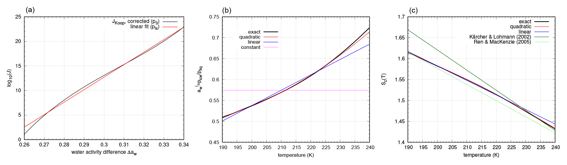
Figure 2 Polynomial approximations of the nucleation rate (a), the ice water activity $a_{\mathrm{w}}^i\left(T\right)=\frac{p_{\mathrm{ice}}\left(T\right)}{p_{\mathrm{liq}}\left(T\right)}$ (b), and the saturation ratio threshold S_c(T) (c), respectively. Panel (b) also includes the approximations by Kärcher and Lohmann (2002) and Ren and Mackenzie (2005).

In contrast, using a least-squares fitting routine for $\mathrm{0.26}\le \mathrm{\Delta }{a}_{\mathrm{w}}\le \mathrm{0.34}$, we obtain a linear function

$$\begin{array}{}\text{(38)}& p_{\mathrm{ls}}\left(x\right)=b_{\mathrm{ls},\mathrm{0}}+b_{\mathrm{ls},\mathrm{1}}\cdot x,\end{array}$$

with $b_{\mathrm{ls},\mathrm{0}}=-\mathrm{62.19267}$ and $b_{\mathrm{ls},\mathrm{1}}=\mathrm{254.7749}$. For further investigations, we only use the linear fit from Eq. (38). We observe that the linear fit p_ls(x) best approximates p₃ close to the inflection point x_infl≈0.30756 (see Fig. 2, left panel).

For each linear approximation $p\left(x\right)=b_{\mathrm{0}}+b_{\mathrm{1}}\cdot x$ of p₃(x), the exponent of the nucleation rate and the saturation ratio threshold become, as demonstrated in Sect. 4.2,

$$\begin{array}{}\text{(39)}& \begin{array}{rl}& j(S_{\mathrm{i}},T)=j_{\mathrm{0}}+\underset{:=A\left(T\right)}{\underbrace{b_{\mathrm{1}}{a}_{\mathrm{w}}^i\left(T\right)}}(S_{\mathrm{i}}-S_{\mathrm{c}}(T\left)\right),\\ & S_{\mathrm{c}}\left(T\right)={\displaystyle \frac{\mathrm{1}}{a_{\mathrm{w}}^i\left(T\right)}}{\displaystyle \frac{j_{\mathrm{0}}-b_{\mathrm{0}}}{b_{\mathrm{1}}}}+\mathrm{1}.\end{array}\end{array}$$

Since $a_{\mathrm{w}}^i$ is a rather complicated function of temperature, it is particularly useful in the context of analytical investigations to have simpler approximations of this quantity. This motivates us to approximate $a_{\mathrm{w}}^i$ and its inverse $\frac{\mathrm{1}}{a_{\mathrm{w}}^i}$ in the relevant temperature range $\mathrm{190}\le T\le \mathrm{230}$ K by polynomials q(T) of degree deg(q)≤2. Similarly, we can approximate the nucleation threshold S_c(T) by polynomials s(T) of degree deg(s)≤2. For the approximations we use a least-squares procedure within the temperature range $\mathrm{190}\le T\le \mathrm{230}$ K. The results are presented in Fig. 2 (middle and right panels).

Combining the approximations q(T) and s(T) yields the formulation

$$\begin{array}{}\text{(40)}& \begin{array}{rl}j(S_{\mathrm{i}},T)& =j_{\mathrm{0}}+b_{\mathrm{1}}q\left(T\right)(S_{\mathrm{i}}-s(T\left)\right)\\ & \approx j_{\mathrm{0}}+A\left(T\right)(S_{\mathrm{i}}-S_{\mathrm{c}}(T\left)\right)\end{array}\end{array}$$

of log ₁₀(J). As can be seen in Fig. 2, the nucleation threshold is accurately approximated by a linear relation (deviation is smaller than 0.3 %). In former studies (e.g. Kärcher and Lohmann, 2002; Ren and Mackenzie, 2005) linear fits were derived for the nucleation thresholds; however, these fits deviate significantly more from the reference in comparison to ours (see Fig. 2). The deviation depends on the respective formulation (or approximation) of $a_{\mathrm{w}}^i$.

4.4 Thresholds for prescribed nucleation rate values

The threshold description in Sect. 4.3 was based on the choice j₀=16, corresponding to a nucleation rate $J={\mathrm{10}}^{\mathrm{16}}{\mathrm{m}}^{-\mathrm{3}}{\mathrm{s}}^{-\mathrm{1}}$. As already mentioned, the choice of j₀ is quite arbitrary, and these high values of J are very often not reached in the numerical simulations (see Sect. 4.5). For a better diagnostics of the nucleation events and the relative strength of nucleation events, we introduce a similar concept for nucleation thresholds, based on a prescribed nucleation rate value $J\sim {\mathrm{10}}^{x_{\mathrm{0}}}$. For this purpose we use Eq. (40) of the nucleation threshold based on the linear approximation of the nucleation rate with a fixed but arbitrary value x₀>0 for the nucleation rate value; hence, we can write

$$\begin{array}{}\text{(41)}& \begin{array}{rl}{x}_{\mathrm{0}}& =j(S_{\mathrm{0}},T)=j_{\mathrm{0}}+A\left(T\right)\left(S_{\mathrm{0}}-S_{\mathrm{c}}\left(T\right)\right)\\ & \iff S_{\mathrm{c}x\mathrm{0}}\left(T\right)=S_{\mathrm{0}}={\displaystyle \frac{x_{\mathrm{0}}-j_{\mathrm{0}}}{A\left(T\right)}}+S_{\mathrm{c}}\left(T\right),\end{array}\end{array}$$

where the function $A\left(T\right)=b_{\mathrm{1}}{a}_{\mathrm{w}}^i\left(T\right)$ only depends on the linear approximation of J, as stated in Sect. 4.2. Note that obviously S_cx0(T)=S_c(T) for x₀=j₀. This leads to the formulation of the nucleation rate

$$\begin{array}{}\text{(42)}& j(S_{\mathrm{i}},T)=x_{\mathrm{0}}+A\left(T\right)\left(S_{\mathrm{i}}-S_{\mathrm{c}x\mathrm{0}}\left(T\right)\right),\end{array}$$

with a general nucleation value x₀ and its associated threshold function S_cx0(T). The threshold function is just shifted by the value $\frac{x_{\mathrm{0}}-j_{\mathrm{0}}}{A\left(T\right)}$; i.e. the type of the threshold function remains the same. This formulation will be used for the theoretical investigations using small perturbations (see Sect. 4.6)

4.5 Numerical simulations of nucleation events for different approximations

In the following we investigate the impact of our approximations of log ₁₀(J) on nucleation events. The setup is as follows: we use the simple bulk ice physics model as described by the set of ordinary differential equations (15), (16), and (17) in Sect. 3. A nucleation event is ensured by assuming a constant vertical velocity, which directly translates into a constant adiabatic cooling of the air parcel and, thus, an initially increasing saturation ratio. Instead of changing the temperature adiabatically, we directly control the supersaturation as described in Sect. 3; this allows us to control the nucleation event without the need to disentangle the different contributions of temperature and supersaturation.

The nucleation event always shows the same qualitative behaviour: due to the supersaturation source ∼wS_i with a constant updraft w, the variable S_i increases, and the nucleation term produces ice crystals, which can grow by water vapour diffusion, constituting a sink for supersaturation. The peak value of S_i is reached once the source and sink of supersaturation balance. Afterwards the variable S_i decreases due to diffusional growth and thus shuts off the nucleation term. The peak value depends crucially on the number of nucleated ice crystals that are needed, to balance the source for S_i by the diffusional growth (depending on the product of number concentration and mean radius of ice crystals). The number concentration of ice crystals produced in the nucleation event clearly depends on the vertical velocity w (source term) and the environmental conditions (diffusion depends on temperature and pressure). For details of the time evolution of nucleation events, see Appendix B.

4.5.1 Standard approximation

We compare the following four different representations of the nucleation rate using numerical simulations:

1. We represent the nucleation rate in the water activity formulation by Koop et al. (2000) with the correction as described in Sect. 4.1 (reference nucleation rate).

2. We represent the water activity approximated by the linear fit as described in Sect. 4.3 (see Eq. 38, linear regression).

3. We represent the nucleation rate as a function of S_i an T as described in Sect. 4.2, based on the formulation

   $$\begin{array}{}\text{(43)}& {\log }_{\mathrm{10}}J=j_{\mathrm{0}}+A\left(T\right)(S_{\mathrm{i}}-S_{\mathrm{c}}(T\left)\right)\end{array}$$

   of the exponent of the nucleation rate. We compare the following two sets of approximations for A(T) and S_c(T):

   • a.

     A linear approximation is used for A(T) and a quadratic approximation for S_c(T), respectively.

   • b.

     A constant approximation is used for A(T) and a linear approximation for S_c(T), respectively.

These are specific cases; however arbitrary combinations of approximations for A(T) and S_c(T) might be used.

Figure 3 Different approximations of nucleation rate for different temperatures (a: T=196 K, b: T=216 K, c: T=236 K). Black – reference nucleation rate; red – linear fit to reference nucleation rate; blue – threshold description due to Eq. (43), using a linear approximation for $a_{\mathrm{w}}^i$ and a quadratic threshold function S_c; green – threshold description due to Eq. (43), using a constant for $a_{\mathrm{w}}^i$ and a linear threshold function S_c.

Figure 3 shows the approximated exponents of the nucleation rate together with the (corrected) reference formulation by Koop et al. (2000) for the three temperatures T=196, 216, and 236 K as functions of Δa_w. These temperatures are chosen for direct comparison with former studies (Kärcher and Lohmann, 2002; Spichtinger and Gierens, 2009). Evidently, the linear fit with respect to water activity is very close to the reference, and the same is true for the case of a linear function A(T) and a quadratic approximation S_c(T). For the simplest approximation (constant function A(T) and linear approximation S_c(T)), larger deviations from the reference nucleation rate can be seen. At T=196 K, there is a strong underestimation in the lower range of Δa_w, whereas for T=236 K the underestimation is most pronounced for higher values of Δa_w (green vs. black curves). In both cases, we expect deviations in the number concentrations of nucleated ice crystals during the nucleation event and the maximum saturation ratio attained.

We investigate standard nucleation events in terms of (i) the resulting ice crystal number concentration at the end of the simulation as in former studies (e.g. Kärcher and Lohmann, 2002; Spichtinger and Gierens, 2009) and (ii) the maximum (peak) supersaturation, which was reached during the nucleation event. Although the latter is usually not considered, it is of interest for comparisons with real measurements, for example, in cloud chambers.

Figure 4 shows the results of the numerical simulations, i.e. the number of nucleated ice crystals (top panel) and the maximum saturation ratio (bottom panel) at environmental pressure p=200 hPa (the results are similar for other environmental conditions).

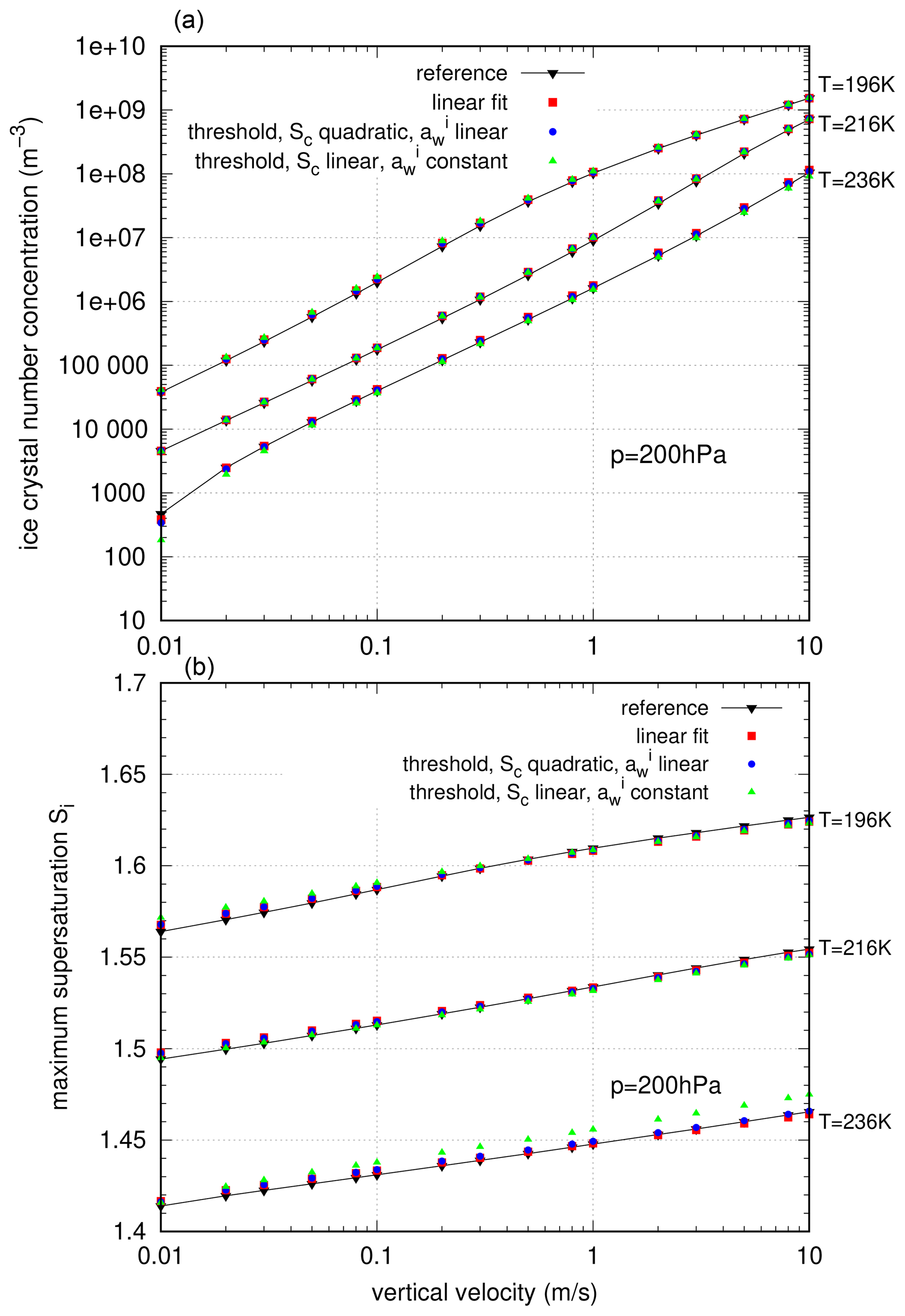
Figure 4 Comparison of different approximations of the nucleation rate by Koop et al. (2000) for standard nucleation events driven by a constant vertical velocity w. (a) Ice crystal number concentration and (b) maximum supersaturation.

Comparing the number of nucleated ice crystals and the maximum saturation ratio, it is evident that the difference between the reference calculation, based on the corrected nucleation rate by Koop et al. (2000), and the simulations using the approximated nucleation rates is rather small.

For almost all nucleation events, the deviation from the reference simulations is not larger than ±15 %. To assess these deviations, one should keep in mind that measurements of ice crystal number concentrations are quite difficult, and the uncertainties are usually larger than 15 %. For instance, for the forward-scattering spectrometer probe instrument, which was used in many flight campaigns (e.g. Voigt et al., 2017), the uncertainty is estimated by about ∼ 10 % (de Reus et al., 2009). Thus, the deviations in our simulations and the uncertainties of realistic measurements are roughly of the same order. This fact renders it presumably impossible to decide on the correctness of any of the different formulations and approximations of the nucleation rate based on the available observations.

Finally, we conclude that a linear approximation of the reference nucleation rate by Koop et al. (2000) is accurate enough to represent nucleation events in a physically meaningful way. Thus, we can use this description as well as the derived formulations of the nucleation rate as a function of temperature T and saturation ratio S_i in order to investigate which parameters of the nucleation rates significantly affect the outcome of nucleation events. This will be carried out in the next section.

4.5.2 Impact of the parameters of the linear approximation

Generally, we are interested in the impact of the formulation of the nucleation rate on nucleation events. The original parameterization by Koop et al. (2000) is based on a cubic polynomial, which has slopes in the range $\mathrm{221}\le b\le \mathrm{453}$; see Sect. 4.3. The linear approximation is sufficiently good for representing the reference rate; thus, we now use this simple linear representation ${\log }_{\mathrm{10}}J=b_{\mathrm{0}}+b_{\mathrm{1}}\cdot \mathrm{\Delta }{a}_{\mathrm{w}}$ in order to test the sensitivity of nucleation events on the two parameters b₀, b₁. Parameter b₀ controls the absolute value of the nucleation rate, while parameter b₁ accounts for its steepness, i.e. the slope.

In a first step, we investigate the impact of the slope of the nucleation rate given by coefficient b₁. One should keep in mind that during the nucleation event, the value of $\mathrm{\Delta }{a}_{\mathrm{w}}=(S_{\mathrm{i}}-\mathrm{1})a_{\mathrm{w}}^i\left(T\right)$ is increasing as S_i increases; thus the exponent of the nucleation rate basically grows linearly. Consequently, an increase in the saturation ratio immediately translates into an increase in Δa_w; hence the abscissa in Fig. 5 may be thought of as representing the saturation ratio. If high values of the nucleation rate are already reached at lower supersaturation values, the nucleation is triggered earlier in comparison to the reference scenario.

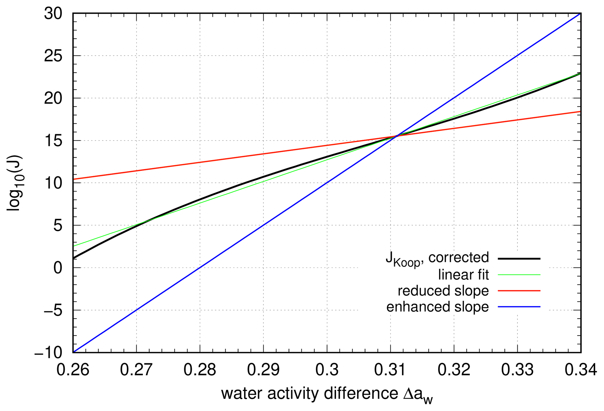
Figure 5 Artificial change in the slope of the linear function in the exponent of the nucleation rate. The fit to the reference curve is indicated by the green line (slope b₁∼250), a reduced slope (b₁∼100) is displayed in red, and an enhanced slope (b₁∼500) is displayed in blue.

However, an earlier onset of ice nucleation implies that the newly nucleated ice crystals already start to grow by diffusion. Consequently, the growing ice crystals tend to decrease the saturation ratio and, if they are sufficiently numerous, prematurely stop the nucleation event. In this case, fewer ice crystals will nucleate, and a smaller maximum saturation ratio will be reached compared to the reference. The opposite mechanism is expected for smaller values of the nucleation ratio in comparison to the reference; i.e. higher ice crystal concentrations will occur together with a larger maximal saturation ratio.

In order to illustrate this mechanism more quantitatively, we artificially changed the slope of the linear function. The reference slope b₁≈255 is either reduced to a value of b₁=100 or enhanced to a value b₁=500, which is motivated by the values of the Taylor approximation, derived in Sect. 4.3. In both cases, the parameter b₀ of the linear function is adapted such that the inflection point of the polynomial p₃(Δa_w) at Δa_w∼0.311 is met for better comparison with the reference simulations. The resulting nucleation rates are displayed in Fig. 5, while the number of nucleated ice crystals and the maximum ice saturation ratio during the nucleation event are summarized in Fig. 6: the top panel shows the concentrations of nucleated ice crystals, and the bottom panel shows the maximum saturation ratio during the nucleation events.

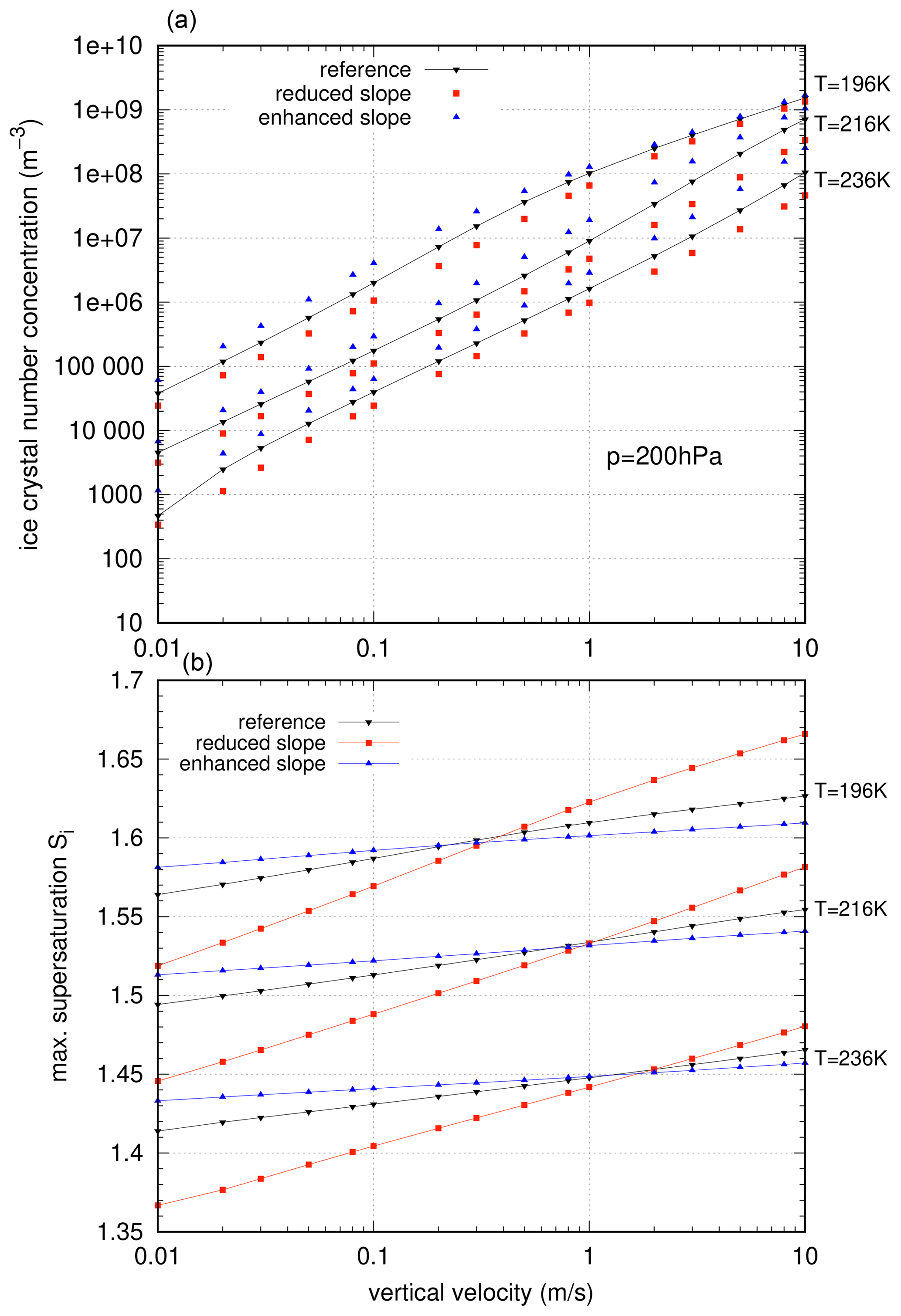
Figure 6 Impact of the slope on the idealized nucleation events. (a) Ice crystal number concentrations and (b) maximum supersaturation values. The colours are chosen as in Fig. 5; i.e. red squares indicate a reduced slope, and blue triangles indicate an enhanced slope, respectively.

In the case of the enhanced or reduced slope, as indicated in Fig. 5, we see the theoretically proposed behaviour in the ice crystal number concentration exactly: the values are reduced for reduced slopes and enhanced for enhanced slopes. The reductions are by up to a factor of 0.4, the enhancements are by up to a factor of 2.4, and the largest changes can be seen at the highest temperature T=236 K.

In the bottom panel of Fig. 6, a dependency on temperature and vertical velocity is seen. For very low vertical velocities, the maximum supersaturation behaves as expected, i.e. reduced values for the reduced slope and enhanced values for the enhanced slope. For very high vertical velocities, this behaviour is reversed; i.e. we see reduced values of S_i,max for enhanced slopes and enhanced values of S_i,max for reduced slopes. The transition slightly depends on the temperature. This can be explained as follows: for low vertical velocities, Δa_w (and thus the supersaturation) is always below the inflection point Δa_w∼0.311. Thus the nucleation rate is always smaller for the enhanced slope in comparison to the reference, while it is always larger in comparison to the reference for the reduced slope. Therefore, in the case of an enhanced slope, the nucleation starts later compared to the reference. This leads to the behaviour as described above. However, beyond the inflection point, the behaviour is reversed, and thus the resulting maximum supersaturation is now enhanced for a reduced slope, and it is reduced for an enhanced slope. The inflection point is reached at different vertical velocities for different temperatures, i.e. for lower temperatures at lower values of w and for higher temperatures at higher values of w. Note that only the maximum supersaturation is affected upon Δa_w crossing the inflection point, while no influence on the number concentration of ice crystals is seen.

After having varied the slope of the nucleation rate, we now turn to its absolute values and modify coefficient b₀, which translates into a change of values of J by ${\mathrm{10}}^{b_{\mathrm{0}}}$. In order to investigate the sensitivity, we add a constant value $\mathrm{\Delta }b\in \mathit{\{}-\mathrm{6},-\mathrm{3},\mathrm{3},\mathrm{6}\mathit{\}}$ to the coefficient b₀, resulting in an increase or decrease in the absolute value of the nucleation rate by a factor of 10^Δb. In Fig. 7 the results in terms of ice crystal number concentration and maximum supersaturation are displayed.

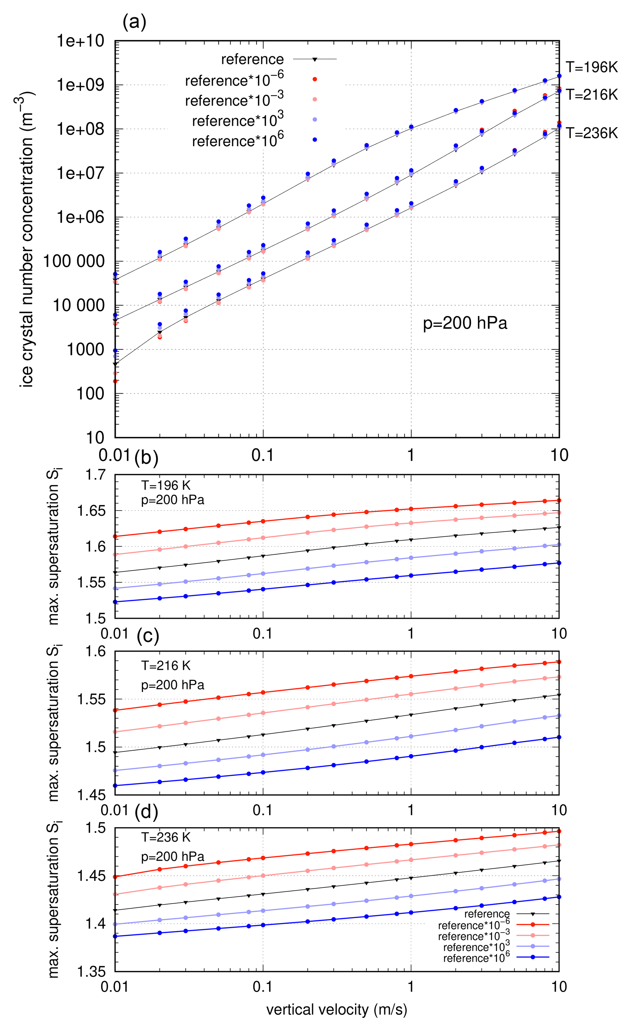
Figure 7 Comparison of ice crystal number concentrations (a) and maximum supersaturation (b–d, temperature T=196, 216, and 236 K) for absolute changes in the nucleation rate by a factor 10^Δb, with $\mathrm{\Delta }b\in \mathit{\{}-\mathrm{6},-\mathrm{3},\mathrm{3},\mathrm{6}\mathit{\}}$.

Maybe surprisingly, the absolute values of the number concentrations of ice crystals in comparison to the reference formulation are not crucially affected (see Fig. 7, top panel), although some deviations occur (up to a factor of 2). The strongest deviations can be seen for warm temperatures (T=236 K) at very low vertical velocities. Overall, the relative deviations from the reference events in variables n_i and peak values of S_i are within the interval [0.4, 2], but for vertical velocities in the range $w\ge \mathrm{0.05}\mathrm{m}{\mathrm{s}}^{-\mathrm{1}}$, the relative deviation is within the interval [0.8, 1.4].

Comparing the influence of a scaling of the absolute values of the nucleation rate and the steepness of the rate, we conclude that the correct steepness of the nucleation rate is much more important than the absolute value of J. Even changes by orders of magnitude in the values of the nucleation rate have a minor impact on the number of nucleated ice crystals. A similar conclusion was also drawn in the theoretical study by Baumgartner and Spichtinger (2019). In that study, the authors investigated a slightly simplified system of equations by means of asymptotic analysis. The simplified system describes the temporal evolution of the number concentration of ice crystals and the saturation ratio, and an approximate asymptotic solution was constructed. To leading order, the approximate solution for the number concentration of ice crystals was completely independent of the precise values of the nucleation rate, but the steepness contributed directly. The only necessary condition on the values of the nucleation rate was that it attains large values, i.e. significantly larger than the other coefficients within the equations.

For the maximum supersaturation values, the impact of the absolute value of J is much more pronounced. As expected, upon reduction of the nucleation rate by a factor of 10^Δb with $\mathrm{\Delta }b\in \mathit{\{}-\mathrm{6},-\mathrm{3}\mathit{\}}$ the supersaturation reaches much higher values of S_i until the values of the rescaled nucleation rate become large enough to initiate the nucleation of ice crystals. For the enhancement of the absolute values of the nucleation rate, the results are reversed: the maximum supersaturation is reduced, since the enhanced nucleation rate attains values that allow for the production of ice crystals for smaller saturation ratios. This behaviour is represented in the bottom panels of Fig. 7.

We remark that this idealized enhancement of the nucleation rate can also be seen in the connection with the aerosol number concentration n_a. A change of n_a by some orders of magnitudes while no changes in J are applied has the same effect as changing the absolute value of the nucleation rate (or the parameter b₀ in the argument of the exponential function). Thus, a strong reduction or enhancement of the available solution droplets will only slightly change the amount of ice crystals in a nucleation event. Therefore, we can conclude that for a meaningful approximation of the nucleation rate, the exact number concentration of available aerosols is also not crucial for the strength of the homogeneous nucleation event but perhaps for the starting time of the event. Including size effects of the solution droplets might additionally change the picture quantitatively (see, for example, Baumgartner et al., 2020).

4.6 Impact of perturbations in S_i and T on the nucleation rate

In this section we investigate the impact of changes in S_i and/or T on the nucleation rate by employing a perturbation analysis. A short explanation of this technique is given in Appendix D. In the real atmosphere, variations of the temperature due to dynamical processes will introduce such changes, for example, from a passing or even breaking gravity wave. In numerical simulations, these variations (also often called fluctuations) are often artificially introduced (e.g. Jensen and Pfister, 2004). In any case, the impact of such changes is investigated using perturbation analysis (also called asymptotic analysis).

We start with the linear approximation of the nucleation rate as formulated in Eq. (40) with $A\left(T\right)=b_{\mathrm{1}}{a}_{\mathrm{w}}^i\left(T\right)$. We can estimate the usual values of the function A(T) in the temperature range $\mathrm{190}\mathrm{K}\le T\le \mathrm{230}$ K using $\mathrm{0.51}\le a_{\mathrm{w}}^i\left(T\right)\le \mathrm{0.66}$ such that $\mathrm{129}\le A\left(T\right)\le \mathrm{169}$. For a very simple but still sufficiently accurate constant approximation of $a_{\mathrm{w}}^i\left(T\right)$, we can set $a_{\mathrm{w}\mathrm{0}}^i=\mathrm{0.574312}$ (see Fig. 2, pink line), such that $A\left(T\right)\approx A_{\mathrm{0}}=b_{\mathrm{1}}{a}_{\mathrm{w}\mathrm{0}}^i=\mathrm{146.32}$. Finally we can state $A\left(T\right)=\mathcal{O}\left({\mathit{\epsilon }}^{-\mathrm{2}}\right)$ with the usual perturbation approach ε∼0.1, such that we set $A\left(T\right)=A^{\ast }{\mathit{\epsilon }}^{-\mathrm{2}}$ with $A^{\ast }=\mathcal{O}\left(\mathrm{1}\right)$ as ε→0. For the non-dimensionalization of the threshold function in the linear approximation $S_{\mathrm{c}}\left(T\right)\approx s_{\mathrm{0}}+s_{\mathrm{1}}T$, we have to estimate the order of the coefficients for the relevant temperature range. Using $\mathrm{190}\mathrm{K}\le T_{\mathrm{ref}}\le \mathrm{230}$ K and the definition T=T_refϑ with the nondimensional temperature ϑ, we find

$$\begin{array}{}\text{(44)}& S_{\mathrm{c}}\left(T\right)=s_{\mathrm{c}}\left(\mathit{\vartheta }\right)=s_{\mathrm{0}}+s_{\mathrm{1}}T=s_{\mathrm{0}}+s_{\mathrm{1}}{T}_{\mathrm{ref}}\mathit{\vartheta }={\mathit{\sigma }}_{\mathrm{0}}-{\mathit{\sigma }}_{\mathrm{1}}\mathit{\vartheta },\end{array}$$

with ${\mathit{\sigma }}_{\mathrm{1}}=-s_{\mathrm{1}}{T}_{\mathrm{ref}}$. Obviously, $s_{\mathrm{0}}={\mathit{\sigma }}_{\mathrm{0}}=\mathrm{2.27697}=\mathcal{O}\left(\mathrm{1}\right)$ and $\mathrm{0.66}\le {\mathit{\sigma }}_{\mathrm{1}}\le \mathrm{0.8}$, such that σ₁=𝒪(1). Using the simplest approximation A(T)=A₀ and $S_{\mathrm{c}}\left(T\right)=s_{\mathrm{0}}+s_{\mathrm{1}}T$ for the general formulation of the threshold function S_cx0 (see Eq. 41), we can simplify the expression as

$$\begin{array}{}\text{(45)}& \begin{array}{rl}{S}_{\mathrm{c}x\mathrm{0}}\left(T\right)& ={\displaystyle \frac{x_{\mathrm{0}}-j_{\mathrm{0}}}{A_{\mathrm{0}}}}+s_{\mathrm{0}}+s_{\mathrm{1}}T\\ & =\underset{=:s_{x\mathrm{0}}}{\underbrace{\left({\displaystyle \frac{x_{\mathrm{0}}-j_{\mathrm{0}}}{A_{\mathrm{0}}}}+s_{\mathrm{0}}\right)}}+s_{\mathrm{1}}T\\ & =s_{x\mathrm{0}}+s_{\mathrm{1}}T.\end{array}\end{array}$$

Using non-dimensionalization, we end up with the following representation:

$$\begin{array}{}\text{(46)}& S_{\mathrm{c}x\mathrm{0}}\left(T\right)=s_{\mathrm{c}x\mathrm{0}}\left(\mathit{\vartheta }\right)=s_{x\mathrm{0}}+s_{\mathrm{1}}T={\mathit{\sigma }}_{x\mathrm{0}}-{\mathit{\sigma }}_{\mathrm{1}}\mathit{\vartheta },\end{array}$$

where σ_x0=s_x0 and ${\mathit{\sigma }}_{\mathrm{1}}=-s_{\mathrm{1}}{T}_{\mathrm{ref}}$. Finally, we use the estimation $A_{\mathrm{0}}=A^{\ast }{\mathit{\epsilon }}^{-\mathrm{2}}$ to obtain

$$\begin{array}{}\text{(47)}& {\mathit{\sigma }}_{x\mathrm{0}}={\left(A^{\ast }\right)}^{-\mathrm{1}}{\mathit{\epsilon }}^{\mathrm{2}}(x_{\mathrm{0}}-j_{\mathrm{0}})+{\mathit{\sigma }}_{\mathrm{0}}=\mathit{\delta }+{\mathit{\sigma }}_{\mathrm{0}}.\end{array}$$

Since $j_{\mathrm{0}}=\mathcal{O}\left({\mathit{\epsilon }}^{-\mathrm{1}}\right)$ and x₀=𝒪(ε^β) with $\mathit{\beta }\ge -\mathrm{1}$, we find ${\mathit{\sigma }}_{x\mathrm{0}}=\mathit{\delta }+{\mathit{\sigma }}_{\mathrm{0}}=\mathcal{O}\left(\mathit{\epsilon }\right)+\mathcal{O}\left(\mathrm{1}\right)=\mathcal{O}\left(\mathrm{1}\right)$. After non-dimensionalizing the argument in the nucleation rate, we can now investigate the response of the nucleation rate upon a perturbation (i) in the saturation ratio (i.e. in the same way as the numerical simulations are set up), (ii) in temperature, and (iii) in adiabatic changes of temperature driving changes in the saturation ratio simultaneously. In reality, case (iii) is almost exclusively relevant.

First, we estimate the increase of J due to variations of S_i at a constant temperature T=T_ref. For this purpose we start at a given value of the saturation ratio S_i, which corresponds to a certain threshold x₀ via the relation (41). We choose this value as a reference value $S_{\mathrm{ref}}=S_{\mathrm{c}x\mathrm{0}}\left(T_{\mathrm{ref}}\right)=s_{\mathrm{c}x\mathrm{0}}\left(\mathrm{1}\right)={\mathit{\sigma }}_{\mathrm{0}}-{\mathit{\sigma }}_{\mathrm{1}}$; this corresponds to a reference value of the nucleation rate $J=J_{\mathrm{ref}}=J_{\mathrm{unit}}\cdot {\mathrm{10}}^{x_{\mathrm{0}}}$ (with $J_{\mathrm{unit}}=\mathrm{1}{\mathrm{m}}^{-\mathrm{3}}{\mathrm{s}}^{-\mathrm{1}}$). Assuming the expansion

$$\begin{array}{}\text{(48)}& S_{\mathrm{i}}=S_{\mathrm{0}}+\mathit{\epsilon }{S}_{\mathrm{1}}+{\mathit{\epsilon }}^{\mathrm{2}}{S}_{\mathrm{2}}+{\mathit{\epsilon }}^{\mathrm{3}}{S}_{\mathrm{3}}+\mathcal{O}\left({\mathit{\epsilon }}^{\mathrm{4}}\right)\end{array}$$

for the saturation ratio, where $S_{\mathrm{0}}=S_{\mathrm{ref}}{\mathit{\sigma }}_{x\mathrm{0}}-{\mathit{\sigma }}_{\mathrm{1}}$, we investigate the impact of such a perturbation on the exponent j. Keeping the temperature fixed as in the numerical simulations, we arrive at

$$\begin{array}{}\text{(49)}& \begin{array}{rl}j(S_{\mathrm{i}},T)& =j(s,t)=x_{\mathrm{0}}+A_{\mathrm{0}}\left(S_{\mathrm{i}}-S_{\mathrm{ref}}\right)\\ & =x_{\mathrm{0}}+A^{\ast }{\mathit{\epsilon }}^{-\mathrm{2}}(S_{\mathrm{ref}}\\ & +\mathit{\epsilon }{S}_{\mathrm{1}}+{\mathit{\epsilon }}^{\mathrm{2}}{S}_{\mathrm{2}}+{\mathit{\epsilon }}^{\mathrm{3}}{S}_{\mathrm{3}}+\mathcal{O}\left({\mathit{\epsilon }}^{\mathrm{4}}\right)-S_{\mathrm{ref}})\\ & =x_{\mathrm{0}}+{\mathit{\epsilon }}^{-\mathrm{1}}{A}^{\ast }{S}_{\mathrm{1}}+A^{\ast }{S}_{\mathrm{2}}+\mathit{\epsilon }{A}^{\ast }{S}_{\mathrm{3}}+\mathcal{O}\left({\mathit{\epsilon }}^{\mathrm{2}}\right).\end{array}\end{array}$$

We are interested in the relative change of the nucleation rates $\frac{J(S_{\mathrm{i}},T)}{J_{\mathrm{ref}}}$, which translates into $j(S_{\mathrm{i}},\mathrm{1})-j(S_{\mathrm{ref}},\mathrm{1})$. By definition, we have $x_{\mathrm{0}}=j(S_{\mathrm{ref}},\mathrm{1})$; thus we obtain

$$\begin{array}{}\text{(50)}& \begin{array}{rl}j(S_{\mathrm{i}},\mathrm{1})-j(S_{\mathrm{ref}},\mathrm{1})=& {\mathit{\epsilon }}^{-\mathrm{1}}{A}^{\ast }{S}_{\mathrm{1}}+A^{\ast }{S}_{\mathrm{2}}+\mathit{\epsilon }{A}^{\ast }{S}_{\mathrm{3}}\\ & +\mathcal{O}\left({\mathit{\epsilon }}^{\mathrm{2}}\right).\end{array}\end{array}$$

Inspecting Eq. (50), it is evident that a nonzero perturbation term S_α in Eq. (48) is connected with the factor ε^α−2; hence a change of order 𝒪(ε^α) in supersaturation translates into a change of order 𝒪(ε^α−2) in the exponent of J. For instance, a change by S_i∼0.01 translates into a change of 𝒪(1) in j and thus in a change by a factor of 10 in the nucleation rate J.

Second, we consider perturbations of temperature without changing the saturation ratio, although this might not happen in the atmosphere. Using the approach above with a constant reference value of saturation, i.e. $S_{\mathrm{ref}}=s_{\mathrm{c}x\mathrm{0}}\left(\mathrm{1}\right)={\mathit{\sigma }}_{\mathrm{0}}-{\mathit{\sigma }}_{\mathrm{1}}$ and temperature perturbations $\mathit{\vartheta }=\mathrm{1}+\mathit{\epsilon }{\mathit{\vartheta }}_{\mathrm{1}}+{\mathit{\epsilon }}^{\mathrm{2}}{\mathit{\vartheta }}_{\mathrm{2}}+{\mathit{\epsilon }}^{\mathrm{3}}{\mathit{\vartheta }}_{\mathrm{3}}+\mathcal{O}\left({\mathit{\epsilon }}^{\mathrm{4}}\right)$, we find the following expression:

$$\begin{array}{}\text{(51)}& \begin{array}{rl}& j(s_{\mathrm{ref}},\mathit{\vartheta })=x_{\mathrm{0}}+A_{\mathrm{0}}\left(S_{\mathrm{ref}}\right.\\ & \left.-\left({\mathit{\sigma }}_{\mathrm{0}}-{\mathit{\sigma }}_{\mathrm{1}}\left(\mathrm{1}+\mathit{\epsilon }{\mathit{\vartheta }}_{\mathrm{1}}+{\mathit{\epsilon }}^{\mathrm{2}}{\mathit{\vartheta }}_{\mathrm{2}}+{\mathit{\epsilon }}^{\mathrm{3}}{\mathit{\vartheta }}_{\mathrm{3}}+\mathcal{O}\left({\mathit{\epsilon }}^{\mathrm{4}}\right)\right)\right)\right)\\ & =x_{\mathrm{0}}+A^{\ast }{\mathit{\epsilon }}^{-\mathrm{2}}\left(\mathit{\epsilon }{\mathit{\vartheta }}_{\mathrm{1}}+{\mathit{\epsilon }}^{\mathrm{2}}{\mathit{\sigma }}_{\mathrm{1}}{\mathit{\vartheta }}_{\mathrm{2}}+{\mathit{\epsilon }}^{\mathrm{3}}{\mathit{\sigma }}_{\mathrm{1}}{\mathit{\vartheta }}_{\mathrm{3}}+\mathcal{O}\left({\mathit{\epsilon }}^{\mathrm{4}}\right)\right)\\ & =x_{\mathrm{0}}+{\mathit{\epsilon }}^{-\mathrm{1}}{A}^{\ast }{\mathit{\sigma }}_{\mathrm{1}}{\mathit{\vartheta }}_{\mathrm{1}}+A^{\ast }{\mathit{\sigma }}_{\mathrm{1}}{\mathit{\vartheta }}_{\mathrm{2}}+\mathit{\epsilon }{A}^{\ast }{\mathit{\sigma }}_{\mathrm{1}}{\mathit{\vartheta }}_{\mathrm{3}}+\mathcal{O}\left({\mathit{\epsilon }}^{\mathrm{2}}\right).\end{array}\end{array}$$

The relative change of the nucleation rate is then given by

$$\begin{array}{}\text{(52)}& \begin{array}{rl}j(S_{\mathrm{ref}},\mathit{\vartheta })-j(S_{\mathrm{ref}},\mathrm{1})=& x_{\mathrm{0}}+{\mathit{\epsilon }}^{-\mathrm{1}}{A}^{\ast }{\mathit{\sigma }}_{\mathrm{1}}{\mathit{\vartheta }}_{\mathrm{1}}+A^{\ast }{\mathit{\sigma }}_{\mathrm{1}}{\mathit{\vartheta }}_{\mathrm{2}}\\ & +A^{\ast }{\mathit{\sigma }}_{\mathrm{1}}{\mathit{\vartheta }}_{\mathrm{3}}\mathit{\epsilon }+\mathcal{O}\left({\mathit{\epsilon }}^{\mathrm{2}}\right).\end{array}\end{array}$$

Thus, a temperature perturbation ϑ_α of order 𝒪(ε^α) leads to a relative change in j of order 𝒪(ε^α−2). Note the sign of the perturbations, which turns into the opposite sign in the change of j. Because of the strictly monotonic decrease of the threshold function S_cx0(T), a negative temperature change leads to a higher threshold and in turn to a lower nucleation rate at a given saturation ratio.

Instead of perturbing the saturation ratio and the temperature individually, these quantities are connected in the real world. To a good approximation, their joint variation is through a purely adiabatic change. Therefore, we finally investigate the impact of adiabatic temperature changes on the saturation ratio and in turn on the nucleation rate. For this purpose, we have to consider the dependence of S_i on adiabatic temperature changes. We start with the cooling source term of the saturation ratio

$$\begin{array}{}\text{(53)}& \mathrm{d}{S}_{\mathrm{i}}=\left({\displaystyle \frac{\mathrm{1}}{\mathit{\kappa }}}-{\displaystyle \frac{L}{R_{\mathrm{v}}T}}\right)S_{\mathrm{i}}{\displaystyle \frac{\mathrm{d}T}{T}}.\end{array}$$

The term $\mathit{\gamma }\left(T\right)=\frac{\mathrm{1}}{\mathit{\kappa }}-\frac{L}{R_{\mathrm{v}}T}$ within the brackets has the values $-\mathrm{28.8}\le \mathit{\gamma }\left(T\right)\le -\mathrm{23.2}$ for $\mathrm{190}\mathrm{K}\le T\le \mathrm{230}$ K, such that we find $\mathit{\gamma }\left(T\right)=\mathcal{O}\left({\mathit{\epsilon }}^{-\mathrm{1}}\right)={\mathit{\gamma }}^{\ast }{\mathit{\epsilon }}^{-\mathrm{1}}$ and ${\mathit{\gamma }}^{\ast }\sim -\mathrm{2.5}<\mathrm{0}$. Approximating the total differential in Eq. (53) with finite differences ΔS_i and ΔT, we arrive at

$$\begin{array}{}\text{(54)}& {\displaystyle \frac{\mathrm{\Delta }{S}_{\mathrm{i}}}{S_{\mathrm{i}}}}={\mathit{\gamma }}^{\ast }{\mathit{\epsilon }}^{-\mathrm{1}}{\displaystyle \frac{\mathrm{\Delta }T}{T}}.\end{array}$$

We set as an approximation S_i=S_ref and T=T_ref, such that we can set

$$\begin{array}{}\text{(55)}& {\displaystyle \frac{\mathrm{\Delta }{S}_{\mathrm{i}}}{S_{\mathrm{ref}}}}={\mathit{\epsilon }}^l{S}_l+\mathcal{O}\left({\mathit{\epsilon }}^{l+\mathrm{1}}\right)=\mathcal{O}\left({\mathit{\epsilon }}^l\right),\end{array}$$

with S_l=𝒪(1). We assume l≥1 since we do not consider changes of the saturation ratio of order 𝒪(1). The analogous expansion for the temperature reads

$$\begin{array}{}\text{(56)}& \begin{array}{rl}& {\displaystyle \frac{\mathrm{\Delta }T}{T_{\mathrm{ref}}}}={\mathit{\epsilon }}^k{\mathit{\vartheta }}_k+\mathcal{O}\left({\mathit{\epsilon }}^{k+\mathrm{1}}\right)=\mathcal{O}\left({\mathit{\epsilon }}^k\right)\\ & \mathrm{with}{\mathit{\vartheta }}_k=\mathcal{O}\left(\mathrm{1}\right)\forall k\ge \mathrm{1}.\end{array}\end{array}$$

Combining these expansions, Eq. (53) becomes

$$\begin{array}{}\text{(57)}& \begin{array}{rl}{\displaystyle \frac{\mathrm{\Delta }{S}_{\mathrm{i}}}{S_{\mathrm{ref}}}}& ={\mathit{\gamma }}^{\ast }{\mathit{\epsilon }}^{-\mathrm{1}}{\displaystyle \frac{\mathrm{\Delta }T}{T_{\mathrm{ref}}}}={\mathit{\gamma }}^{\ast }{\mathit{\epsilon }}^{-\mathrm{1}}\left({\mathit{\epsilon }}^k{\mathit{\vartheta }}_k+\mathcal{O}\left({\mathit{\epsilon }}^{k+\mathrm{1}}\right)\right)\\ & ={\mathit{\gamma }}^{\ast }{t}_k{\mathit{\epsilon }}^{k-\mathrm{1}}+\mathcal{O}\left({\mathit{\epsilon }}^k\right)\end{array}\end{array}$$

or equivalently

$$\begin{array}{}\text{(58)}& {\mathit{\epsilon }}^l{S}_l=\mathrm{\Delta }{S}_{\mathrm{i}}=S_{\mathrm{ref}}{\mathit{\gamma }}^{\ast }{\mathit{\vartheta }}_k{\mathit{\epsilon }}^{k-\mathrm{1}}+\mathcal{O}\left({\mathit{\epsilon }}^k\right).\end{array}$$

The only non-trivial balance is achieved for $l=k-\mathrm{1}$; i.e.

$$\begin{array}{}\text{(59)}& S_{k-\mathrm{1}}=S_{\mathrm{ref}}{\mathit{\gamma }}^{\ast }{\mathit{\vartheta }}_k\iff S_k=S_{\mathrm{ref}}{\mathit{\gamma }}^{\ast }{\mathit{\vartheta }}_{k+\mathrm{1}}.\end{array}$$

Note that $l=k-\mathrm{1}\ge \mathrm{1}$; i.e. we have to consider k≥2 for the perturbation of temperature. This is a meaningful restriction since we are interested in small changes of temperature in the cold temperature regime, i.e. a change in the temperature in the order of ∼1 K in physical units. Hence, we would not expect adiabatic temperature changes of order 𝒪(ε), corresponding to changes of order ∼10 K. Thus, we assume an asymptotic expansion

$$\begin{array}{}\text{(60)}& \mathit{\vartheta }=\mathrm{1}+{\mathit{\epsilon }}^{\mathrm{2}}{\mathit{\vartheta }}_{\mathrm{2}}+{\mathit{\epsilon }}^{\mathrm{3}}{\mathit{\vartheta }}_{\mathrm{3}}+\mathcal{O}\left({\mathit{\epsilon }}^{\mathrm{4}}\right)\end{array}$$

for the temperature perturbation. We are generally interested in adiabatic expansions due to vertical upward motion, which in turn leads to decreasing temperatures; hence we conclude ϑ_k<0 for k≥2. Since ${\mathit{\gamma }}^{\ast }<\mathrm{0}$, Eq. (59) leads to positive changes in the saturation ratio s_k>0 for ϑ_k<0. Generally, warming due to adiabatic compression can be studied in the same way by setting ϑ_k>0.

Now we consider the nucleation rate in the formulation for arbitrary thresholds x₀ in the nucleation rate using $S_{\mathrm{ref}}={\mathit{\sigma }}_{x\mathrm{0}}-{\mathit{\sigma }}_{\mathrm{1}}=s_{\mathrm{c}x\mathrm{0}}\left(\mathrm{1}\right)$:

$$\begin{array}{}\text{(61)}& \begin{array}{rl}j(S_{\mathrm{i}},T)& =j(S_{\mathrm{i}},t)=x_{\mathrm{0}}+A^{\ast }{\mathit{\epsilon }}^{-\mathrm{2}}\left(S_{\mathrm{i}}-s_{\mathrm{c}x\mathrm{0}}\left(\mathit{\vartheta }\right)\right)\\ & =x_{\mathrm{0}}+A^{\ast }{\mathit{\epsilon }}^{-\mathrm{2}}\left(S_{\mathrm{ref}}+\mathit{\epsilon }{S}_{\mathrm{1}}+{\mathit{\epsilon }}^{\mathrm{2}}{S}_{\mathrm{2}}+{\mathit{\epsilon }}^{\mathrm{3}}{S}_{\mathrm{3}}\right.\\ & \left.-\left({\mathit{\sigma }}_{x\mathrm{0}}-{\mathit{\sigma }}_{\mathrm{1}}\left(\mathrm{1}+{\mathit{\epsilon }}^{\mathrm{2}}{\mathit{\vartheta }}_{\mathrm{2}}+{\mathit{\epsilon }}^{\mathrm{3}}{\mathit{\vartheta }}_{\mathrm{3}}\right)\right)+\mathcal{O}\left({\mathit{\epsilon }}^{\mathrm{4}}\right)\right)\\ & =x_{\mathrm{0}}+A^{\ast }{\mathit{\epsilon }}^{-\mathrm{2}}\left(\mathit{\epsilon }{S}_{\mathrm{1}}+{\mathit{\epsilon }}^{\mathrm{2}}{S}_{\mathrm{2}}+{\mathit{\epsilon }}^{\mathrm{3}}{S}_{\mathrm{3}}+{\mathit{\epsilon }}^{\mathrm{2}}{\mathit{\sigma }}_{\mathrm{1}}{\mathit{\vartheta }}_{\mathrm{2}}\right.\\ & \left.+{\mathit{\epsilon }}^{\mathrm{3}}{\mathit{\sigma }}_{\mathrm{1}}{\mathit{\vartheta }}_{\mathrm{3}}+\mathcal{O}\left({\mathit{\epsilon }}^{\mathrm{4}}\right)\right)\\ & =x_{\mathrm{0}}+A^{\ast }{\mathit{\epsilon }}^{-\mathrm{2}}\left(\mathit{\epsilon }{S}_{\mathrm{ref}}{\mathit{\gamma }}^{\ast }{\mathit{\vartheta }}_{\mathrm{2}}+{\mathit{\epsilon }}^{\mathrm{2}}{S}_{\mathrm{ref}}{\mathit{\gamma }}^{\ast }{\mathit{\vartheta }}_{\mathrm{3}}\right.\\ & \left.+{\mathit{\epsilon }}^{\mathrm{3}}{S}_{\mathrm{ref}}{\mathit{\gamma }}^{\ast }{\mathit{\vartheta }}_{\mathrm{4}}+{\mathit{\epsilon }}^{\mathrm{2}}{\mathit{\sigma }}_{\mathrm{1}}{\mathit{\vartheta }}_{\mathrm{2}}+{\mathit{\epsilon }}^{\mathrm{3}}{\mathit{\sigma }}_{\mathrm{1}}{\mathit{\vartheta }}_{\mathrm{3}}+\mathcal{O}\left({\mathit{\epsilon }}^{\mathrm{4}}\right)\right)\\ & =x_{\mathrm{0}}+A^{\ast }{\mathit{\epsilon }}^{-\mathrm{2}}\left(\mathit{\epsilon }{S}_{\mathrm{ref}}{\mathit{\gamma }}^{\ast }{\mathit{\vartheta }}_{\mathrm{2}}+{\mathit{\epsilon }}^{\mathrm{2}}\left(S_{\mathrm{ref}}{\mathit{\gamma }}^{\ast }{\mathit{\vartheta }}_{\mathrm{3}}+{\mathit{\sigma }}_{\mathrm{1}}{\mathit{\vartheta }}_{\mathrm{2}}\right)\right.\\ & \left.+{\mathit{\epsilon }}^{\mathrm{3}}\left(S_{\mathrm{ref}}{\mathit{\gamma }}^{\ast }{\mathit{\vartheta }}_{\mathrm{4}}+{\mathit{\sigma }}_{\mathrm{1}}{\mathit{\vartheta }}_{\mathrm{3}}\right)+\mathcal{O}\left({\mathit{\epsilon }}^{\mathrm{4}}\right)\right)\\ & =x_{\mathrm{0}}+A^{\ast }{S}_{\mathrm{ref}}{\mathit{\gamma }}^{\ast }{\mathit{\vartheta }}_{\mathrm{2}}{\mathit{\epsilon }}^{-\mathrm{1}}+A^{\ast }\left(S_{\mathrm{ref}}{\mathit{\gamma }}^{\ast }{\mathit{\vartheta }}_{\mathrm{3}}+{\mathit{\sigma }}_{\mathrm{1}}{\mathit{\vartheta }}_{\mathrm{2}}\right)\\ & +A^{\ast }\left(s_{\mathrm{ref}}{\mathit{\gamma }}^{\ast }{\mathit{\vartheta }}_{\mathrm{4}}+{\mathit{\sigma }}_{\mathrm{1}}{\mathit{\vartheta }}_{\mathrm{3}}\right)\mathit{\epsilon }+\mathcal{O}\left({\mathit{\epsilon }}^{\mathrm{2}}\right).\end{array}\end{array}$$

Thus, for k≥2 we find terms of the form $A^{\ast }\left(s_{\mathrm{ref}}{\mathit{\gamma }}^{\ast }{\mathit{\vartheta }}_{k+\mathrm{1}}+{\mathit{\sigma }}_{\mathrm{1}}{\mathit{\vartheta }}_k\right){\mathit{\epsilon }}^{k-\mathrm{2}}$ of order 𝒪(ε^k−2). Comparing the nucleation rates, we find for the relative change

$$\begin{array}{}\text{(62)}& \begin{array}{rl}& j(S_{\mathrm{i}},T)-j(S_{\mathrm{ref}},T_{\mathrm{ref}})\\ & =j(S_{\mathrm{i}},t)-j(S_{\mathrm{ref}},\mathrm{1})\\ & =A^{\ast }{S}_{\mathrm{ref}}{\mathit{\gamma }}^{\ast }{\mathit{\vartheta }}_{\mathrm{2}}{\mathit{\epsilon }}^{-\mathrm{1}}+A^{\ast }\left(S_{\mathrm{ref}}{\mathit{\gamma }}^{\ast }{\mathit{\vartheta }}_{\mathrm{3}}+{\mathit{\sigma }}_{\mathrm{1}}{\mathit{\vartheta }}_{\mathrm{2}}\right)\\ & +A^{\ast }\left(S_{\mathrm{ref}}{\mathit{\gamma }}^{\ast }{\mathit{\vartheta }}_{\mathrm{4}}+{\mathit{\sigma }}_{\mathrm{1}}{t}_{\mathrm{3}}\right)\mathit{\epsilon }+\mathcal{O}\left({\mathit{\epsilon }}^{\mathrm{2}}\right).\end{array}\end{array}$$

For the relative impact of these terms, we use the estimations ${\mathit{\gamma }}^{\ast }<-\mathrm{2.3}$ and σ₁≤0.8. We have to distinguish two scenarios for perturbations ϑ_k<0:

1. ϑ_k<0 for all k≥2. In this case we can assume

   $$\begin{array}{}\text{(63)}& S_{\mathrm{ref}}{\mathit{\gamma }}^{\ast }{\mathit{\vartheta }}_{k+\mathrm{1}}+{\mathit{\sigma }}_{\mathrm{1}}{\mathit{\vartheta }}_k>\mathrm{0}.\end{array}$$

   Therefore, an adiabatic temperature perturbation ϑ_k of order 𝒪(ε^k) (k≥2) leads to relative changes in j of order 𝒪(ε^k−3). Note that the changes in saturation ratio are always dominant and larger than the changes in the threshold, which changes j by order 𝒪(ε^k−2) in the opposite direction.

2. ϑ_k<0 and ${\mathit{\vartheta }}_{k+\mathrm{1}}=\mathrm{0}$ for a distinct k≥2. In this case, the previously discussed temperature effect can be seen; i.e. the nucleation threshold is changed, leading to a reduction of the nucleation rate exponent. This effect is merely academic, since we have to switch off higher perturbations in temperature, which is quite unlikely.

One should keep in mind that we investigated the relative increase in the exponent of the nucleation rate. A relative change of order 𝒪(ε^k) in the exponent translates into a relative change of order ​​​​​​​$\mathcal{O}\left({\mathrm{10}}^{{\mathit{ϵ}}^k}\right)$ in the nucleation rate J, thus ranging over several orders of magnitudes. For instance, in the first scenario, changes of temperature of order ∼1K lead to changes in j of about ∼10, which in turn translate into a change of the nucleation rate J by a factor of 10¹⁰.

Overall, we can state that changes in S_i are most important for changing j, either stemming from adiabatic temperature changes or driven directly as in our numerical studies.

5 Impact of saturation vapour pressure formulation

Since the formulation of the nucleation rate by Koop et al. (2000) relies on the water activity, and thus on the function $a_{\mathrm{w}}^i\left(T\right)=\frac{p_{\mathrm{ice}}\left(T\right)}{p_{\mathrm{liq}}\left(T\right)}$, the saturation vapour pressure over liquid water (i.e. in no man's land) plays an important role. In this section we investigate the impact of choosing another formulation for p_liq(T) on the nucleation rate and thus on the nucleation events.

5.1 New representation of saturation water vapour

In the formulation by Murphy and Koop (2005), the extrapolation of the saturation vapour pressure into the no man's land of the phase diagram of water is based on the assumption that the state of amorphous ice is thermodynamically equivalent to super-cooled liquid water. Therefore, the specific heat of liquid water can be extended in the super-cooled regime using measurements of amorphous ice. This leads to the established formulation in Murphy and Koop (2005).

Recently, a new representation of the saturation vapour pressure over super-cooled liquid water was proposed by Nachbar et al. (2019). In this study, the authors consider different states of water in the low temperature range. They conclude that amorphous ice is thermodynamically different from super-cooled water; thus they provide a different extrapolation for the saturation vapour pressure (Nachbar et al., 2019).

Although the deviation between the two curves is very small – even in the low temperature range less than 10 % – its impact on saturation ratios as well as on the nucleation thresholds is quite large, as can be seen in Fig. 8.

Figure 8 Water saturation $\left(S_{\mathrm{i}}=\frac{p_{\mathrm{liq}}}{p_{\mathrm{ice}}}\right)$ and nucleation threshold (for $J={\mathrm{10}}^{\mathrm{16}}{\mathrm{m}}^{-\mathrm{3}}{\mathrm{s}}^{-\mathrm{1}}$) for different formulations of saturation vapour pressure over super-cooled water – Murphy and Koop (2005) vs. Nachbar et al. (2019).

The curves of water saturation as well as the nucleation thresholds are systematically shifted to higher values. In addition, the new curves have a more linear shape than the curves resulting from Murphy and Koop (2005). The ratio of the saturation pressures over ice and liquid (i.e. the functions $a_{\mathrm{w}}^i\left(T\right)$ and $\frac{\mathrm{1}}{a_{\mathrm{w}}^i\left(T\right)}$ behave differently), $a_{\mathrm{w}}^i\left(T\right)$, is much closer to a quadratic curve, as can be seen in the top panel of Fig. 9. These new fits were used for the formulation of the approximated nucleation rate. Thus, we do not change the general approach for approximating the nucleation rate, etc.; we only use a different representation of the function $a_{\mathrm{w}}^i\left(T\right)$.

Figure 9 (a) Function $a_{\mathrm{w}}^i\left(T\right)=\frac{p_{\mathrm{ice}}\left(T\right)}{p_{\mathrm{liq}}\left(T\right)}$ (black line) and polynomial approximations (red – quadratic, blue – linear, and pink – constant). (b) Nucleation threshold S_c(T) (black line) and polynomial approximations (red – quadratic and blue – linear). Note that the former approximation by Kärcher and Lohmann (2002) (dark green) is now very close to the new formulation, whereas the fit by Ren and Mackenzie (2005) (turquoise) deviates significantly.

5.2 Numerical simulations of nucleation events

In Fig. 10 the results of the nucleation events using the new representation of the saturation vapour pressure due to Nachbar et al. (2019) are shown. As for former experiments, the ice crystal number concentration (top panel) and the maximum supersaturation values (bottom panel) are shown.

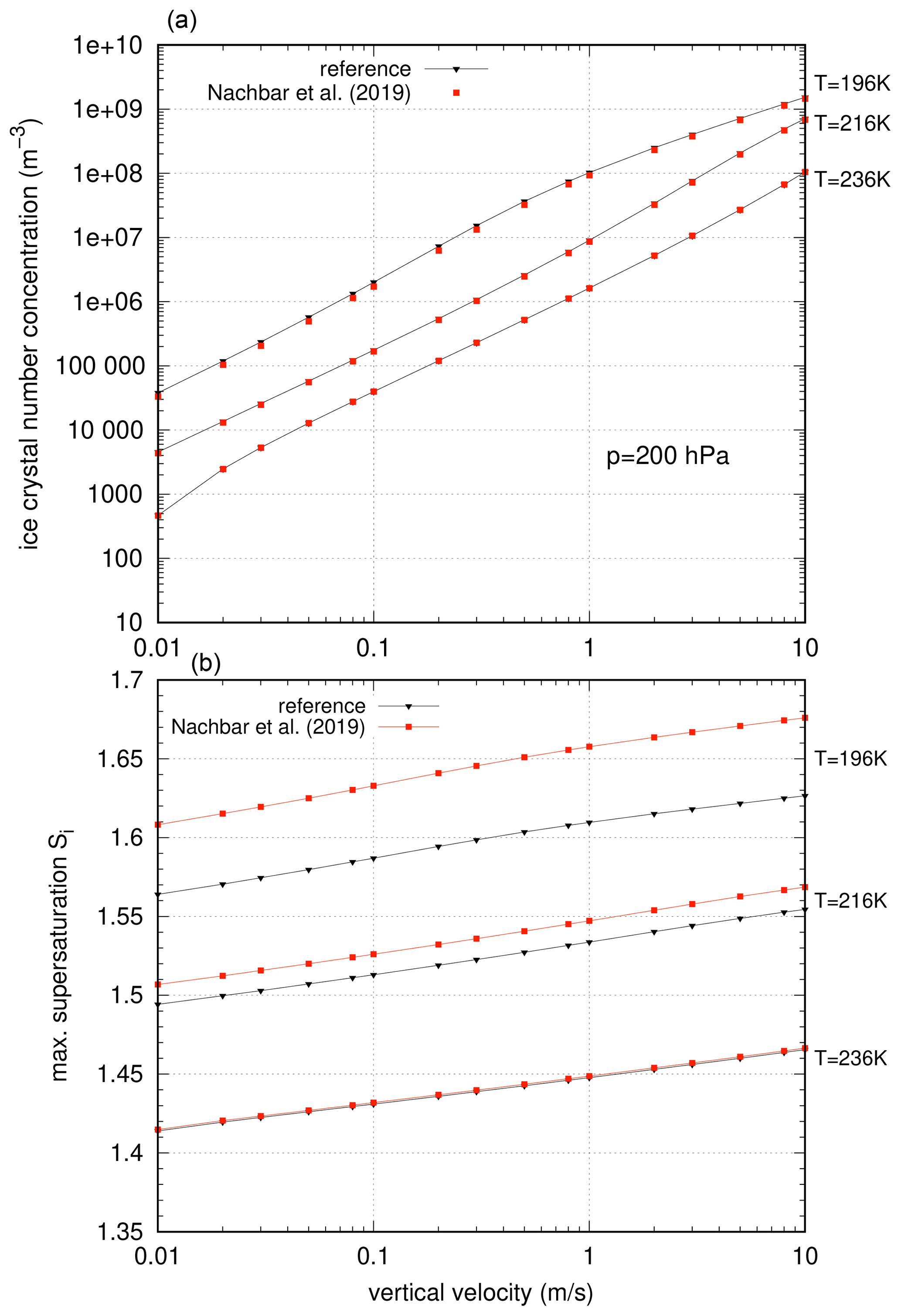
Figure 10 Impact of the formulation of the saturation vapour pressure by Nachbar et al. (2019) on the idealized nucleation events. (a) Ice crystal number concentrations and (b) maximum supersaturation values. The relative differences in number concentrations are always smaller than 15 %.

For the ice crystal number concentration, the impact of the new formulation of p_liq is small; the relative deviation from the reference simulations using the original vapour pressure formulation by Murphy and Koop (2005) is always smaller than 15 %. The deviation increases with decreasing temperature and is most prominent for lower vertical updrafts ($w<\mathrm{1}\mathrm{m}{\mathrm{s}}^{-\mathrm{1}}$).

For the maximum saturation ratio, the change as compared to the reference simulations is much more prominent. As can be seen in Fig. 8 the nucleation thresholds for a value of $J={\mathrm{10}}^{\mathrm{16}}{\mathrm{m}}^{-\mathrm{3}}{\mathrm{s}}^{-\mathrm{1}}$ are increasing with decreasing temperature with a larger slope compared to the reference case. This behaviour can clearly be seen in the maximum supersaturation; for decreasing temperature the maximum supersaturation is increasing to higher values in comparison to the reference simulations (Fig. 10, bottom panel). The increase does not depend on the vertical velocities.

We remark that at the moment it is not clear which thermodynamic hypothesis and thus which resulting approximation for the saturation vapour pressure over liquid water is physically correct; however the formulation by Murphy and Koop (2005) seems to agree with recent measurements (Pathak et al., 2021). In particular, it is not clear if the formulation of Nachbar et al. (2019) can be extrapolated to values T<200 K. Thus, we cannot recommend using a certain formulation.

6 Another approach to formulate the nucleation rate

Up to now we have always employed the reference nucleation rate in our computations, i.e. the formulation as in Koop et al. (2000) but corrected by a constant offset (see Sect. 4.1), in order to match the nucleation rate for pure water droplets by Koop and Murray (2016) in a certain temperature range. In this section we take a different point of view, assuming that we can just directly adopt the formulation by Koop and Murray (2016) for the nucleation rate of aqueous solution droplets, providing an exact match of both curves by definition. In the following we discuss the consequences of using such a direct approach in terms of nucleation events.

6.1 Direct fit to nucleation rate of pure water

In order to arrive at a direct fit, we assume that at water saturation, the freezing of pure water droplets should behave as the freezing of solution droplets at super-cooled states. To avoid a complicated reformulation of the formula from Koop and Murray (2016), in terms of the water activity Δa_w, we use a quadratic polynomial fit to the original formulation J_hom(T) at water saturation; see Appendix C for details. Figure 11 presents the original data (black curve) together with the quadratic fit (red curve) and the corrected formulation of Koop et al. (2000) (blue curve) from Sect. 4.1. In contrast to the (corrected) formulation by Koop et al. (2000), the nucleation rate reaches a maximum at Δa_w∼0.345 and decreases afterwards. As a result, there is a significant deviation between the two nucleation rates (J_K2000>J_KM2016) for the range Δa_w>0.32. Thus, we can expect that for cold temperatures and/or high upward motions, there will be large deviations in the ice crystal number concentrations produced within nucleation events.

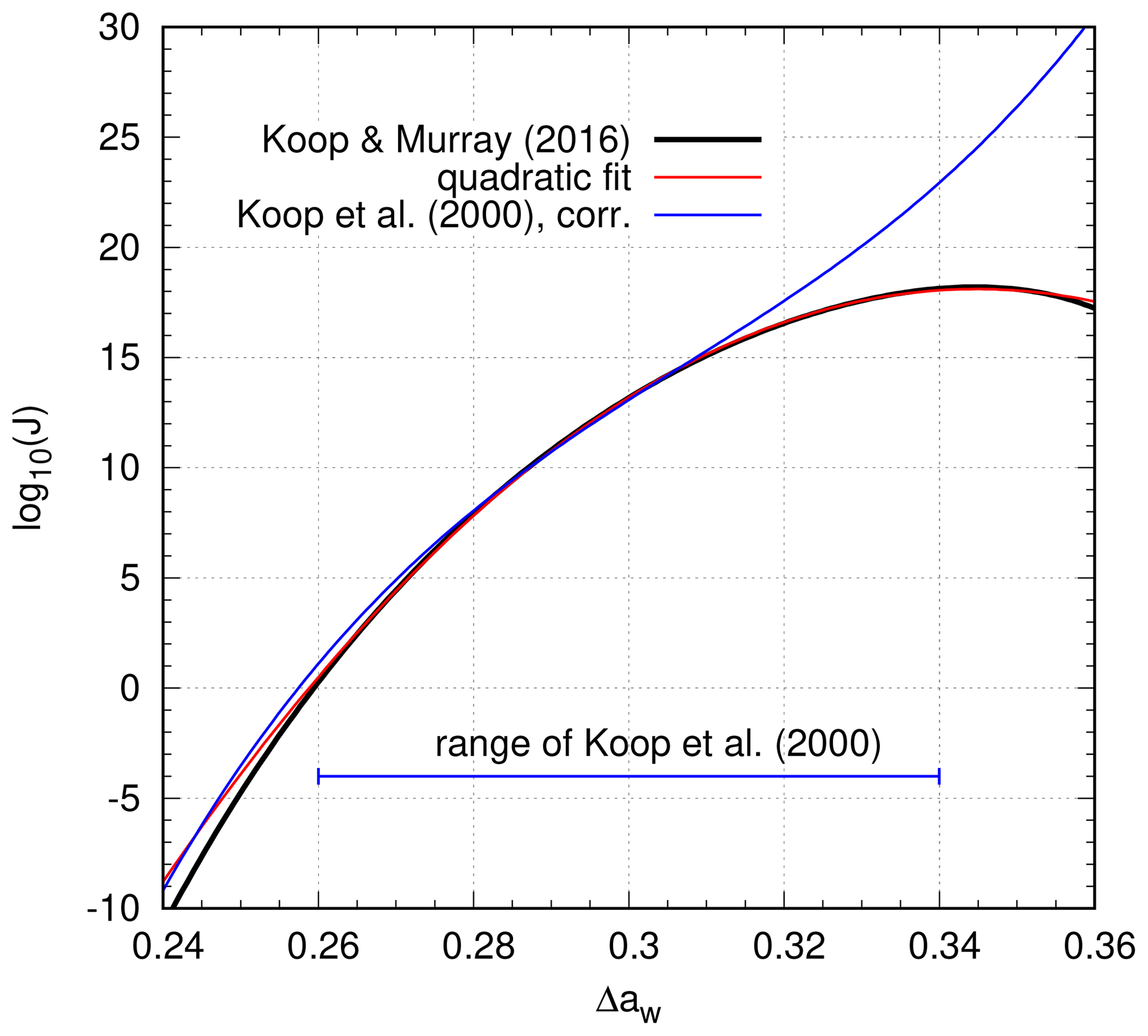
Figure 11 Freezing rate of water droplets (Koop and Murray, 2016, black), a polynomial fit (red), and the nucleation rate of solution droplets (Koop et al., 2000, corrected, blue), all depending on Δa_w.

It should be kept in mind that the range of the parameterization of the nucleation rate as given in Koop et al. (2000) is restricted to the interval $\mathrm{0.26}\le \mathrm{\Delta }{a}_{\mathrm{w}}\le \mathrm{0.34}$. As a result, it is not clear if the parameterization works well for values Δa_w>0.34. However, there are measurements (see Laksmono et al., 2015) for the freezing of pure water droplets that also show a kind of plateau at cold temperatures (corresponding to high values of Δa_w). Thus, for higher values Δa_w>0.34, we use the value J_KM2016(Δa_w)=J_KM2016(0.34) to (a) mimic the plateau in the measurements and (b) avoid numerical issues in the simulations. Assuming that the nucleation rate does not depend on quantities other than water activity, it may now be used in numerical simulations of homogeneous nucleation events.

6.2 Numerical simulations of nucleation events

After having obtained the direct formulation of the nucleation rate of Koop and Murray (2016), we now investigate its impact on nucleation events using numerical simulations as before. For completeness, two different types of simulations are done: (1) simulations using the standard formulation of p_liq by Murphy and Koop (2005) and (2) simulations using the new formulation of p_liq by Nachbar et al. (2019). The results of the simulations are shown in Fig. 12.

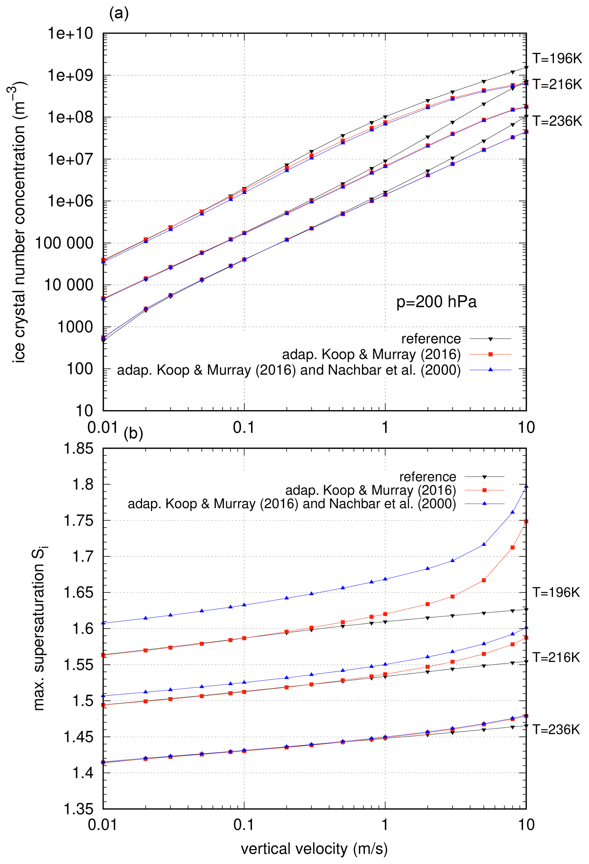
Figure 12 Impact of the direct formulation of the nucleation rate based on Koop and Murray (2016) on the idealized nucleation events. Black triangles and lines indicate the reference simulation, red squares and lines denote the use of the nucleation rate based on Koop and Murray (2016), and blue squares and lines represent the use of the nucleation rate based on Koop and Murray (2016) together with the saturation vapour pressure due to Nachbar et al. (2019). (a) Ice crystal number concentrations and (b) maximum supersaturation values.

First we consider the ice crystal number concentrations (top panel). For low vertical updrafts, the values of n_i are only slightly affected in case of using the adapted nucleation rate. For higher vertical velocities, there is a reduction in the produced ice crystal number concentrations; this reduction increases with increasing vertical updrafts. This effect can be explained as follows. The nucleation rates differ significantly for higher values Δa_w≥0.31; i.e. the slope of the adapted rate is (much) smaller than the original nucleation rate by Koop et al. (2000). For higher updrafts, the supersaturation reaches higher values, which is equivalent to higher values of Δa_w. Thus, the nucleation rates differ for these high updraft events, and fewer ice crystals are produced when using the adapted nucleation rate. Apart from the influence at high vertical velocities, there is almost no difference in the ice crystal number concentrations between the nucleation events using the different formulations.

Considering the values of maximum supersaturation (bottom panel), there is a similar behaviour as for n_i. At low vertical velocities there is almost no difference between the reference nucleation rate and the newly adapted rate. In the case of using the saturation vapour pressure according to Nachbar et al. (2019), the observed shift in the maximum supersaturation values stems from the increased difference between the values of the saturation vapour pressures at low temperatures; see Sect. 5. At higher updrafts ($w>\mathrm{0.5}\mathrm{m}{\mathrm{s}}^{-\mathrm{1}}$), the maximum supersaturation values increase nonlinearly. For the coldest temperature (T=196 K), we note a dramatic increase up to very high values ($S_{\mathrm{i},\max }\sim \mathrm{1.8}$). However, note that in all cases the values of the maximum supersaturation stays below water saturation; hence no liquid origin ice formation would occur.

7 Thresholds of ice nucleation

For the evaluation of measurements of ice clouds, the possible range of supersaturation is often estimated using the so-called Koop line, i.e. the supersaturation threshold S_c(T) which corresponds to a nucleation rate value $J={\mathrm{10}}^{\mathrm{16}}{\mathrm{m}}^{-\mathrm{3}}{\mathrm{s}}^{-\mathrm{1}}={\mathrm{10}}^{\mathrm{10}}{\mathrm{cm}}^{-\mathrm{3}}{\mathrm{s}}^{-\mathrm{1}}$. In many investigations (see, for example, Krämer et al., 2009), this function is used as an upper bound for possible values of S_i inside and also outside of ice clouds. However, from our investigations in this study so far, we have to carefully consider two different aspects from a purely theoretical point of view:

1. The nucleation threshold assigned to the frequently used value j₀=16 is arbitrary chosen; there is no convincing physical justification for using this particular value. In Koop et al. (2000) different values $J={\mathrm{10}}^{j_{\mathrm{0}}}{\mathrm{m}}^{-\mathrm{3}}{\mathrm{s}}^{-\mathrm{1}}$, with $j_{\mathrm{0}}\in [\mathrm{1},\mathrm{17}]$, are used, but for testing the impact of droplet sizes, they used the value j₀=16. Nucleation of ice crystals is not a switching process; it occurs gradually and smoothly, although the nucleation rates are very steep functions of the supersaturation. The size or strength of the nucleation event cannot be determined just by the maximum of the supersaturation; the amount of ice crystals as formed in the nucleation event is determined by the integral over the supersaturation curve (see, for example, the discussion in Dinh et al., 2016). Thus, it is possible to form many crystals in lower updrafts, even if the high nucleation threshold is not reached. From our simulations, we observe that the peak supersaturation for nucleation events depends crucially on the vertical velocity, i.e. on the temperature rate, which is prescribed during the event. This is quite obvious from the differential equation determining the change of S_i: the peak value is given by $\frac{\mathrm{d}{S}_{\mathrm{i}}}{\mathrm{d}t}=\mathrm{0}$, i.e. when source and sink terms balance each other. Since the source includes the vertical velocity linearly, the dependence of the peak supersaturation on w is obvious, although it is not linear.

2. As described above in Sect. 5, it is still not clear which formulation of the saturation vapour pressure is physically correct. However, the use of the formulation by Nachbar et al. (2019) leads to a higher saturation vapour pressure and thus to a higher nucleation threshold, even for arbitrary values j₀ and its associated nucleation threshold S_cx0(T).

Taking these two aspects into account, we can observe the following behaviour. In Fig. 13 (top panel), we compare the nucleation thresholds for the saturation vapour pressure according to Murphy and Koop (2005) for j₀=10 (red curve) and j₀=16 (dark blue curve), with the range of peak supersaturations for vertical velocities $\mathrm{0.01}\mathrm{m}{\mathrm{s}}^{-\mathrm{1}}\le w\le \mathrm{2}\mathrm{m}{\mathrm{s}}^{-\mathrm{1}}$ (black vertical bar) and the maximum value for a very unrealistic value $w=\mathrm{10}\mathrm{m}{\mathrm{s}}^{-\mathrm{1}}$ (black crosses). For comparison, the well-known Koop line as fit and proposed by Kärcher and Lohmann (2002) is plotted (light blue curve). It is quite obvious that for typical vertical velocity values the “classical” Koop line is not reached; i.e. the peak supersaturation is below the threshold. Nevertheless, for strong cooling rates (very high vertical velocities), as are used in experiments in cloud chambers, high supersaturations are reached, which still partly remain below the Koop line. If we change the saturation vapour pressure to the formulation by Nachbar et al. (2019), the qualitative picture remains the same (bottom panel in Fig. 13): even for high vertical updrafts the high nucleation rates are reached; for moderate and small updrafts, the peak supersaturation stays well below the classical nucleation threshold. However, the nucleation thresholds are generally shifted to higher values of supersaturation due to the different saturation vapour pressure formulation. It seems that these values fit better to the experiments in the AIDA cloud chamber as reported in Baumgartner et al. (2022) and Schneider et al. (2021). This might be interpreted as a hint that the formulation by Nachbar et al. (2019) might be the more appropriate formulation for the saturation vapour pressure, although the formulation by Murphy and Koop (2005) agrees well with recent measurements (Pathak et al., 2021). In any case, one has to consider the impact of the cooling rate on the peak supersaturation in a nucleation event. Therefore, the use of the Koop line in the currently applied way is misleading and does not correspond to the actual physics of nucleation events. Note that the temperature-dependent threshold is used in some parameterizations of ice clouds in climate and numerical weather prediction models (see, for example, Kärcher et al., 2006; Köhler and Seifert, 2015). A simple but albeit more realistic extension of such schemes would be a threshold depending on both vertical velocity w and temperature T; a 2D fit to the maximum supersaturation data from our simulations might be a first attempt in this direction.

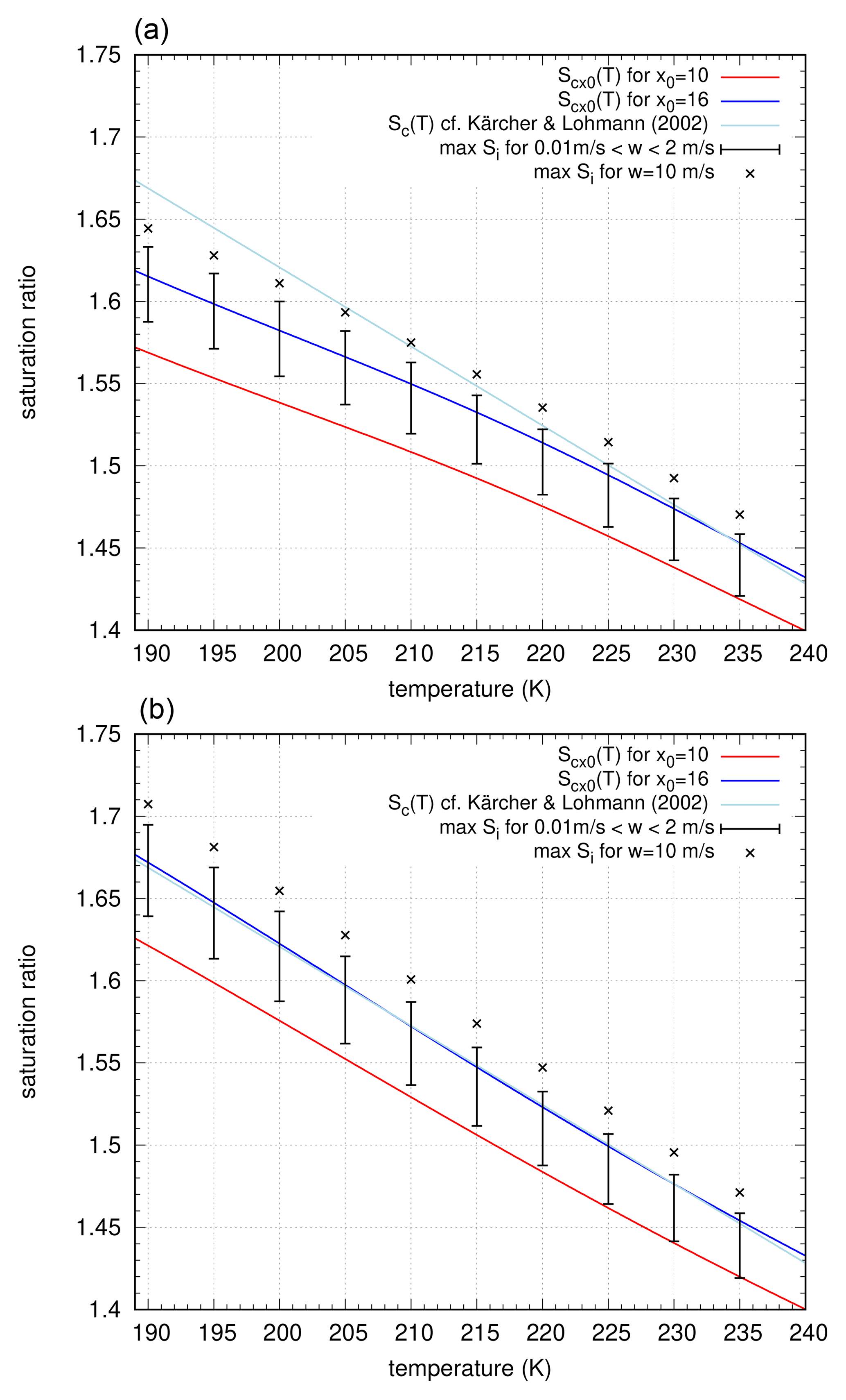
Figure 13 Comparison of nucleation thresholds (red curve: x₀=10, blue curve x₀=16) and the classical Koop line (light blue curve). The black vertical bars indicate the range of peak supersaturation ratios within the nucleation events, computed using vertical velocities ranging from 0.01 to 2 m s⁻¹. The black cross corresponds to the peak supersaturation ratio for the vertical velocity of 10 m s⁻¹. (a) Curves based on the water activity using the saturation vapour pressure formulation by Murphy and Koop (2005) and (b) the same for the saturation vapour pressure formulation by Nachbar et al. (2019).

Finally, we can also investigate the peak supersaturation values for the new empirical nucleation rate formulation, as derived in Sect. 6.1. Generally, we see the same behaviour as for the reference simulations, with a monotonic increase of peak supersaturation values with increasing vertical velocity (see Fig. 14). The use of the saturation vapour pressure formulation by Nachbar et al. (2019) additionally enhances the peak values as seen before. However, the peak values for cold temperatures and very high vertical velocities are strongly enhanced in comparison with the reference simulations. Also these high values are still in line with the measurements in the AIDA chamber, as reported by Baumgartner et al. (2022) and Schneider et al. (2021).

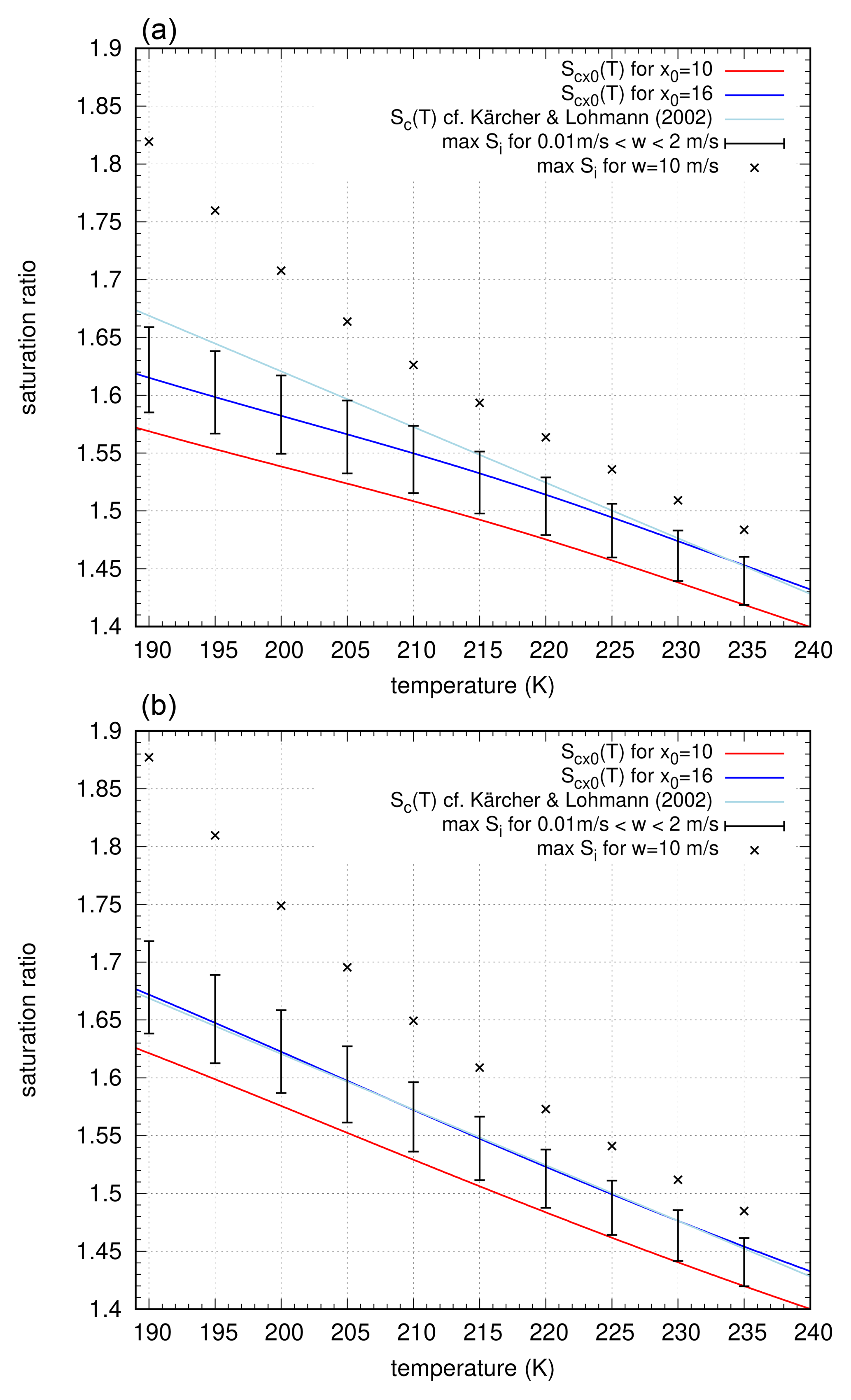
Figure 14 Same as in Fig. 13 but using the nucleation rate as empirically derived in Sect. 6.1. (a) Curves based on the water activity using the saturation vapour pressure formulation by Murphy and Koop (2005) and (b) the same for the saturation vapour pressure formulation by Nachbar et al. (2019).

8 Summary and outlook

We have investigated the impact of the representation of nucleation rates and diffusional growth on idealized nucleation events, as driven by a constant vertical updraft (i.e. a constant cooling rate). In a first step, we have investigated the original formulation of the nucleation rate for homogeneous freezing of aqueous solution droplets in the formulation by Koop et al. (2000); for a better agreement with the nucleation rate of pure water droplets, a simple shift could be applied. For analytical purposes and simple model calculations, a less complicated formulation is desired. We showed that a linear fit to the original formulation depending on the difference in water activity $\mathrm{\Delta }{a}_{\mathrm{w}}=a_{\mathrm{w}}-a_{\mathrm{w}}^i$ is accurate enough to reproduce the ice crystal number concentrations quantitatively. Based on this linearization approach, we derived a threshold formulation of the nucleation rate, which can be used for analytical investigations, as already presented in Baumgartner and Spichtinger (2019). Again, the new formulations are good enough to represent nucleation events quantitatively as compared to the reference nucleation formulation.

Using the linear approximation as a starting point, we investigated the impact of different formulations on idealized nucleation events, changing the two relevant parameters (slope and constant offset). These investigations led to the first major results:

• The absolute values of the nucleation rate only have a marginal impact on the resulting ice crystal number concentrations in a nucleation event. Even a scaling by up to 6 orders of magnitudes did not severely affect the resulting number concentrations. However, the maximum supersaturations changed, and the resulting deviations range up to a few percent of relative humidity. In addition, the time of nucleation onset is slightly shifted.

• The slope of the nucleation rate (or more precisely in the argument of the exponential function) has a much larger impact on the resulting nucleation event and the ice crystal number concentration. Variations in the slope change the number concentrations in the nucleation events by up to a factor of 2.5 (in both directions). Also, the maximum supersaturation is affected by a deviation of a few percent of relative humidity.

As a final conclusion of this part of our work, we can state that the shape of the nucleation rate is of high importance for the representation of the nucleation process, whereas the absolute strength of the rate is almost negligible, if the values are high enough. This shows that the nucleation process (homogeneous freezing of solution droplets) itself is a quite robust process; thus the accurate formulation is maybe less critical than we thought. Also the amount of available solution droplets as controlled by the background aerosol does not affect the nucleation events itself; it can be seen as a scaling factor of the nucleation rate, in the same sense as in the sensitivity analysis of changing the absolute values of nucleation rates. As long as the amount of aerosol particles is some orders of magnitude larger than the ice crystal number concentration as predicted for a nucleation event, this does not play a role for the nucleation events, and we do not have to care about exhausting the reservoir of solution droplets.

We also investigated the impact of a recently published formulation of the water saturation pressure based on a thermodynamic assumption of different phases of water in the very low temperature range (Nachbar et al., 2019). This new formulation leads to changes in the function $a_{\mathrm{w}}^i$, which directly affected the nucleation rate based on Δa_w. Following the derivations of the threshold description, approximations were constructed. The new resulting functions $a_{\mathrm{w}}^i\left(T\right)$ and S_c(T) can be accurately approximated with polynomials of smaller degrees, as compared to the standard formulation. The new formulation of p_liq only marginally changed the resulting ice crystal number concentrations. However, the impact on the maximum supersaturations increased with decreasing temperature up to few percent of relative humidity. Overall, the two different representations of the saturation vapour pressure over liquid water produced very similar, even almost identical, results. Thus, a decision about the validity of a certain formulation must be left to extensive experimental measurements.

In a more speculative part of the study, we adapted the nucleation rate of homogeneous freezing of pure water droplets (Koop and Murray, 2016) as a new parameterization for homogeneous freezing of aqueous solution droplets. This representation is quite similar for low values of Δa_w to the original formulation by Koop et al. (2000) and its approximations. However, for very high water activities (i.e. high supersaturations as driven by large vertical updrafts), there is a significant deviation from the reference nucleation rate. Thus, for some cases in the parameter space (high updrafts and low temperatures), there is a significant deviation in the number concentrations and, more obviously, in the maximum supersaturations, which almost reach water saturation in some cases. This approach showed that the shape of the nucleation rate is important for the resulting nucleation events; strong deviations of the shape from its reference affect the results of the nucleation event significantly. Whether this representation of the nucleation rate is a more accurate approximation to the actual physics of ice nucleation remains an open question and might be an objective for experimental investigations.

Finally, we investigated the commonly used threshold for homogeneous nucleation (Koop line) in the light of peak supersaturation values during nucleation events. This threshold corresponds to a nucleation rate of $J={\mathrm{10}}^{\mathrm{16}}{\mathrm{m}}^{-\mathrm{3}}{\mathrm{s}}^{-\mathrm{1}}$ but is only rarely reached during nucleation events. Nucleation itself starts usually at much lower values of S_i, corresponding to lower values of the nucleation rate. The peak supersaturation during a nucleation event, characterized as an equilibrium between sources and sinks of supersaturation, depends on temperature and vertical velocity. The peak supersaturation is a much more physical quantity to investigate the strength of a nucleation event. The peak supersaturation as diagnosed from the numerical simulations might be a more physical representation of ice nucleation in coarse-resolution models in comparison to the frequently used nucleation threshold.

It should be emphasized that all the results and conclusions are meant in a bulk sense, i.e. for a large collection of ice crystals such as a newly forming cirrus cloud. If one is interested in the details of ice formation for a single or only a small number of particles, then all details of the nucleation rate might be equally important. In that respect, our study shows that homogeneous cirrus formation is a robust physical process.

Appendix A: Model description – details

In this appendix, we present the details of the model as used for the numerical simulations of the nucleation events. Note that we use the mathematical (and also programming) notation of logarithms; i.e. log denotes the natural logarithm (to base e).

A1 Background aerosol

For the aqueous solution droplets in the tropopause region, we assume a size distribution of log-normal type:

$$\begin{array}{}\text{(A1)}& f_{\mathrm{sol}}\left(r\right)={\displaystyle \frac{n_{\mathrm{a}}}{\sqrt{\mathrm{2}\mathit{\pi }}\log {\mathit{\sigma }}_r}}\exp \left(-{\displaystyle \frac{\mathrm{1}}{\mathrm{2}}}{\left({\displaystyle \frac{\log (r/r_{\mathrm{sol}})}{\log {\mathit{\sigma }}_r}}\right)}^{\mathrm{2}}\right){\displaystyle \frac{\mathrm{1}}{r}}\end{array}$$

with a modal radius $r_{\mathrm{sol}}=\mathrm{75}\cdot {\mathrm{10}}^{-\mathrm{9}}\mathrm{m}$ and a geometric standard deviation σ_r=1.5. These values are adapted from the more complex model by Spichtinger and Gierens (2009), using the fact that the dry aerosol population, as used in Spichtinger and Gierens (2009), has grown to larger sizes by water vapour uptake (i.e. assuming Köhler theory; see, for example, Köhler, 1936). The mean volume of the solution droplets

$$\begin{array}{}\text{(A2)}& V_{\mathrm{d}}=V_{\mathrm{sol}}={\displaystyle \frac{\mathrm{4}}{\mathrm{3}}}\mathit{\pi }{r}_{\mathrm{sol}}^{\mathrm{3}}\cdot \exp \left({\displaystyle \frac{\mathrm{9}}{\mathrm{2}}}{\left(\log {\mathit{\sigma }}_r\right)}^{\mathrm{2}}\right)\end{array}$$

is calculated from the third moment of the log-normal distribution.

A2 Mass distribution for ice crystals

For the ice crystals, we assume a mass distribution of log-normal type

$$\begin{array}{}\text{(A3)}& f\left(m\right)={\displaystyle \frac{n_{\mathrm{i}}}{\sqrt{\mathrm{2}\mathit{\pi }}\log {\mathit{\sigma }}_m}}\exp \left(-{\displaystyle \frac{\mathrm{1}}{\mathrm{2}}}\left({\displaystyle \frac{\log (m/m_m)}{\log {\mathit{\sigma }}_m}}\right)\right){\displaystyle \frac{\mathrm{1}}{m}}\end{array}$$

with a parameter

$$\begin{array}{}\text{(A4)}& r_{\mathrm{0}}=\exp \left((\log {\mathit{\sigma }}_m{)}^{\mathrm{2}}\right),\stackrel{\mathrm{‾}}{m}=m_m\sqrt{r_{\mathrm{0}}}=\mathrm{3}\end{array}$$

representing the width of the distribution, as described in Spichtinger and Gierens (2009). This distribution is used for the derivation of the rates in the system of ordinary differential equations for the mean quantities of ice mass and number concentration. The integration of weighting functions of the type $m^k,k\in {\mathbb{R}}_{+}$ leads to general moments, which can be computed analytically:

$$\begin{array}{}\text{(A5)}& \begin{array}{rl}\mathit{\mu }[m{]}_k& :=\underset{\mathrm{0}}{\overset{\mathrm{\infty }}{\int }}{m}^{k}f\left(m\right)\mathrm{d}m\\ & =n_{\mathrm{i}}\cdot m_m^k\exp \left({\displaystyle \frac{\mathrm{1}}{\mathrm{2}}}{\left(k\log {\mathit{\sigma }}_m\right)}^{\mathrm{2}}\right)\\ & =n_{\mathrm{i}}\cdot {\stackrel{\mathrm{‾}}{m}}^k{r}_{\mathrm{0}}^{\frac{k(k-\mathrm{1})}{\mathrm{2}}}.\end{array}\end{array}$$

Note that for the averaged quantities, we obtain n_i=μ[m]₀, q_i=μ[m]₁, respectively. Thus, we use a double-moment scheme in our model.

A3 Diffusion constant

For the diffusion of water vapour in dry air, we use the following expression

$$\begin{array}{}\text{(A6)}& D_{\mathrm{v}}=D_{\mathrm{v}\mathrm{0}}{\left({\displaystyle \frac{T}{T_{\mathrm{0}}}}\right)}^{\mathrm{1.94}}\left({\displaystyle \frac{p_{\mathrm{0}}}{p}}\right),\end{array}$$

which is an empirical fit to measurement data (Hall and Pruppacher, 1976). Note that the valid temperature range is different in the book (Pruppacher and Klett, 2010) and in the original article (Hall and Pruppacher, 1976). For analytical investigations, a representation using a quadratic temperature dependence constitutes a good approximation for a restricted temperature range. For the kinetic correction, we use the function

$$\begin{array}{}\text{(A7)}& f_D(r,a,b)={\displaystyle \frac{\mathrm{1}}{\frac{r}{r+a}+\frac{b}{r}}}={\displaystyle \frac{r^{\mathrm{2}}+ar}{r^{\mathrm{2}}+br+ab}},\end{array}$$

where r denotes the radius of the ice crystal (using a bulk density of ice ${\mathit{\rho }}_{\mathrm{b}}=\mathrm{0.81}\mathrm{kg}{\mathrm{m}}^{-\mathrm{3}}$), and the parameters are given by

$$\begin{array}{}\text{(A8)}& a=\mathit{\lambda }\cdot C_{\mathrm{cunn}},b={\displaystyle \frac{\mathrm{4}{D}_{\mathrm{v}}}{{\mathit{\alpha }}_m{\stackrel{\mathrm{‾}}{c}}_{\mathrm{v}}}}\end{array}$$

using the mean free path of water molecules in air λ (acc. to Pruppacher and Klett, 2010), the Cunningham correction factor C_cunn=0.7, and the mean velocity of water molecules ${\stackrel{\mathrm{‾}}{c}}_{\mathrm{v}}$. We set the accommodation coefficient α_m=0.5 for comparison with former investigations (Kärcher and Lohmann, 2002); this value is also within the range as recommended in recent work by Skrotzki et al. (2013).

For representing the growth rates for the ensemble of ice crystals, by comparison with numerical integration we find that using a shifted mean mass $m_{\mathrm{1}}=c_{\mathrm{1}}\cdot \stackrel{\mathrm{‾}}{m}$, c₁≈0.819 in the kinetic correction function $f(r_{\mathrm{1}},a,b)$ is a good approximation.

A4 Howell factor

Latent heat release due to phase changes during diffusional growth changes the surface temperature of the ice crystal. For taking this into account, we use the Howell factor

$$\begin{array}{}\text{(A9)}& \begin{array}{rl}{G}_{\mathrm{v}}& ={\left[\left({\displaystyle \frac{L}{R_{v}T}}-\mathrm{1}\right){\displaystyle \frac{L}{T}}{\displaystyle \frac{D_{\mathrm{v}}^{\ast }}{K_T^{\ast }}}+{\displaystyle \frac{R_{v}T}{p_{\mathrm{si}}}}\right]}^{-\mathrm{1}}\\ & \approx {\left[\left({\displaystyle \frac{L}{R_{v}T}}-\mathrm{1}\right){\displaystyle \frac{L}{T}}{\displaystyle \frac{D_{\mathrm{v}}}{K_T}}+{\displaystyle \frac{R_{v}T}{p_{\mathrm{si}}}}\right]}^{-\mathrm{1}}.\end{array}\end{array}$$

In the approximation, we neglect the kinetic corrections for diffusion coefficient D_v and heat conductivity of air K_T.

A5 Capacity of ice crystals

For ice crystals, we assume spherical shape for small crystals and columnar shape for large crystals as in Spichtinger and Gierens (2009); thus the shape factor, or capacity, can be determined exactly using the electrostatic analogy (McDonald, 1963), using a prolate spheroid with semi axes a and b; the capacity can be analytically expressed by

$$\begin{array}{}\text{(A10)}& C={\displaystyle \frac{L{\mathit{ϵ}}^{\prime }}{\log \left(\frac{\mathrm{1}+{\mathit{ϵ}}^{\prime }}{\mathrm{1}-{\mathit{ϵ}}^{\prime }}\right)}}\end{array}$$

using the eccentricity ${\mathit{ϵ}}^{\prime }=\sqrt{\mathrm{1}-{\left(\frac{b}{a}\right)}^{\mathrm{2}}}$ and the length L of the crystal, which in turn is a function of the crystal mass. Note that the eccentricity changes with crystal growth since the aspect ratio is changing (see Spichtinger and Gierens, 2009, their Eq. 17). We find a very good approximation to the piece-wise definition of the capacity by Spichtinger and Gierens (2009) depending on the ice crystal mass

$$\begin{array}{}\text{(A11)}& C\left(m\right)\approx a_{\mathrm{1}}\cdot m^{b_{\mathrm{1}}}+a_{\mathrm{2}}\cdot m^{b_{\mathrm{2}}}\end{array}$$

with constants

$$\begin{array}{}\text{(A12)}& \begin{array}{rl}{a}_{\mathrm{1}}& =\mathrm{0.015755}\mathrm{m}{\mathrm{kg}}^{\frac{\mathrm{1}}{{\mathrm{b}}_{\mathrm{1}}}},b_{\mathrm{1}}=\mathrm{0.3},\\ a_{\mathrm{2}}& =\mathrm{0.33565}\mathrm{m}{\mathrm{kg}}^{\frac{\mathrm{1}}{{\mathrm{b}}_{\mathrm{2}}}},b_{\mathrm{2}}=\mathrm{0.43}.\end{array}\end{array}$$

The representation of the capacity in the ice crystal ensemble is given by the integration, leading to general moments $\mathit{\mu }[m{]}_{b_i}$.

A6 Ventilation correction

The empirical ventilation corrections usually depend on the use of two dimensionless numbers, i.e. the Schmidt number N_Sc and the Reynolds number N_Re

$$\begin{array}{}\text{(A13)}& N_{\mathit{Sc}}={\displaystyle \frac{\mathit{\mu }}{D_{\mathrm{v}}\mathit{\rho }}},N_{\mathit{Re}}={\displaystyle \frac{\mathit{\rho }}{\mathit{\mu }}}{v}_{\mathrm{t}}L\end{array}$$

using the dynamic viscosity of air μ (e.g. Dixon, 2007). Thus, the size of the ice crystal L is influencing the Reynolds number via the product v_t(m)L, using the terminal velocity v_t for an ice crystal of mass m. The effect of ventilation, i.e. the additional uptake of water vapour by the airflow around the particle, crucially depends on the shape of the particles. For columnar-shaped ice crystals, we adapt the empirical quadratic fit by Liu et al. (2003) to the simulation data (Ji and Wang, 1999) as follows:

$$\begin{array}{}\text{(A14)}& f_{\mathrm{v}}=\mathrm{1}+c_{\mathit{\chi }}\cdot {\mathit{\chi }}^{\mathrm{2}},c_{\mathit{\chi }}=\mathrm{0.14856},\mathit{\chi }=N_{\mathit{Sc}}^{\frac{\mathrm{1}}{\mathrm{3}}}{N}_{\mathit{Re}}^{\frac{\mathrm{1}}{\mathrm{2}}}.\end{array}$$

For the formulation of the terminal velocity of columnar-shaped ice crystals, v_t(m), we use the formulation by Spichtinger and Gierens (2009), including also the correction for temperature and pressure, respectively. For representing the ensemble of ice crystals, by comparison with the numerical integration, we find that using a shifted mean mass $m_{\mathrm{2}}=c_{\mathrm{2}}\cdot \stackrel{\mathrm{‾}}{m}$ with c₂=1.5 in the formulation of the Reynolds number leads to a very good agreement.

Appendix B: Reference simulation results

In this section we report on the results of the reference simulations, using the corrected formulation of the nucleation rate for super-cooled aqueous solution droplets by Koop et al. (2000). For evaluating the quality of the simplified model, we compare the number concentration of ice crystals as obtained from standard nucleation events with results from literature, i.e. with a model using sophisticated particle physics (Kärcher and Lohmann, 2002) and a complex bulk physics scheme (Spichtinger and Gierens, 2009). In Fig. B1 the results are represented for the temperatures T=196, 216, and 236 K at pressure p=200 hPa, as prescribed in Kärcher and Lohmann (2002).

In comparison, we see an overall good agreement of our simple model with the more sophisticated models (Kärcher and Lohmann, 2002; Spichtinger and Gierens, 2009). However, we have to remark here that the deviation in the results for temperature T=236 K at low vertical velocities is the result of the neglect of the ventilation correction in the model by Kärcher and Lohmann (2002). In summary, our simplified approach compares very well with the results of the other studies.

In Fig. B2 a typical nucleation event is shown. Here, two different nucleation parameterizations are used, the reference by Koop et al. (2000) (black line) and the linear fit (red line). There are small differences in the time evolution of the variables saturation ratio S_i (left panel), number concentration n_i (middle panel), and mean mass m (right panel), but in general there is the same behaviour in both cases.

The source of supersaturation (i.e. cooling by vertical updraft and adiabatic expansion) leads to an increase in S_i until nucleation starts at about t_start∼40 s, i.e. at very low values of the nucleation rate. S_i is still increasing since the sink of depositional growth is not strong enough to reduce water vapour efficiently; thus, the ice crystal number concentration is further increasing due to permanent ice nucleation. At the peak supersaturation, the source and sink of supersaturation are balanced (t_peak∼110 s); after this time, S_i is decreasing due to the dominant growth term. The number concentration does not change much from this time on, but as long as the values of S_i are large enough, ice nucleation still takes place. At about t∼125 s the nucleation event is complete, and no further nucleation takes place, since the nucleation rate is too small. Note that during the time interval [t_start,t_peak] the mean mass m is almost constant (this feature is more prominent in the linear fit case), whereas for t>t_peak the mass increases. For t<t_peak the nucleation is dominant; thus diffusional growth just compensates for the number increase by mass, whereas afterwards crystal growth is dominant over nucleation. This feature was already seen in former investigations, which leads to a model reduction for analytical investigations (Baumgartner and Spichtinger, 2019). The different nucleation parameterizations agree qualitatively for a nucleation event; however, the nonlinear reference rate leads to some variations. While for the linear fit case, the increase in n_i is approximately an exponential growth n_i(t)∼exp (αt), and in turn the mean mass is almost constant in the relevant time interval, for the reference case the change deviates slightly from exponential growth.

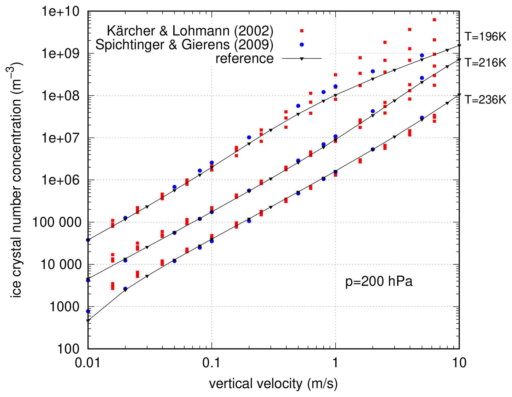
Figure B1 Comparison of ice crystal number concentrations as obtained for typical nucleation events from different models. Red squares – particle model by Kärcher and Lohmann (2002); blue circles – complex two moment bulk scheme by Spichtinger and Gierens (2009); and black line and triangles – simpler bulk model from this study, indicated as new reference.

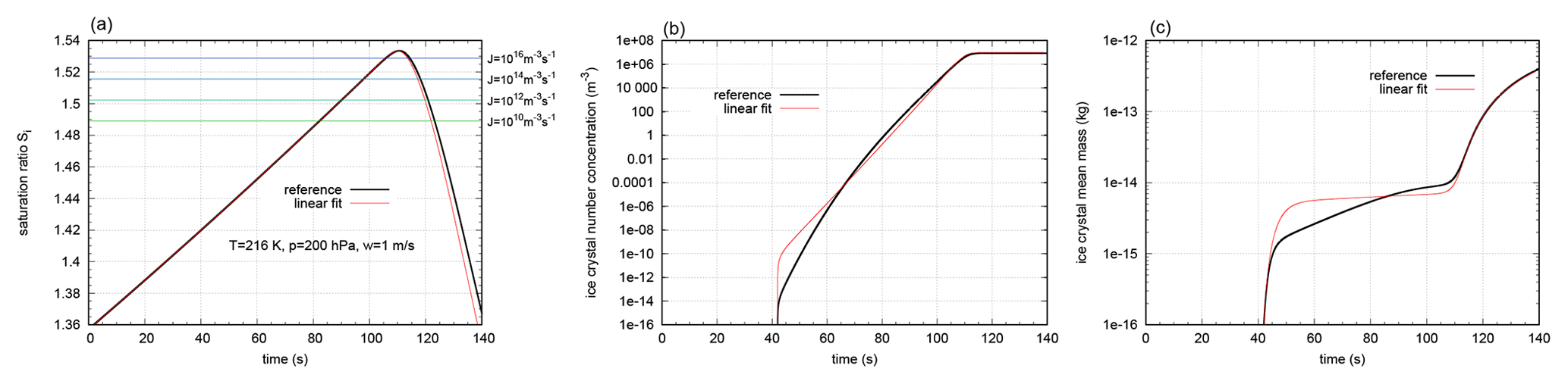
Figure B2 Representative example for a typical nucleation event for temperature T=216 K and pressure p=200 hPa with a forcing of $w=\mathrm{1}\mathrm{m}{\mathrm{s}}^{-\mathrm{1}}$. Red line – reference nucleation rate after Koop et al. (2000) and black line – nucleation rate approximated by linear function as given in Eq. (38). (a) Saturation ratio, (b) ice crystal number concentration, and (c) mean mass.

Note that the thresholds of constant nucleation rates in Fig. B2 (left panel) can be calculated from Eq. (39) using the respective values for j₀ (i.e. $j_{\mathrm{0}}\in \mathit{\{}\mathrm{10},\mathrm{12},\mathrm{14},\mathrm{16}\mathit{\}}$) in the formulation of the supersaturation threshold.

Appendix C: Simple fit for nucleation rate of pure water droplets

In Koop and Murray (2016) a polynomial of degree 6 is used for fitting the experimental values of the nucleation rate for pure super-cooled water. Since polynomials of high degree are difficult to evaluate numerically, we present fits with polynomials of lower degrees, which are still accurate in the relevant temperature range. The original formulation of the nucleation rate is

$$\begin{array}{}\text{(C1)}& \begin{array}{rl}& J_{\mathrm{hom}}\left(T\right)={\mathrm{10}}^{p_n\left(x\right)},p_n\left(x\right)=\sum _{i=\mathrm{0}}^n{c}_i\cdot x^i,\\ & x=T-T_{\mathrm{m}}.\end{array}\end{array}$$

with a polynomial p_n(x) of degree n=6 using the melting temperature of pure water T_m=273.15 K. The coefficients c_i are reported in Koop and Murray (2016, Table VII), where the nucleation rate is given in units of cubic centimetres per second (${\mathrm{cm}}^{-\mathrm{3}}{\mathrm{s}}^{-\mathrm{1}}$). We reformulate the nucleation rate in SI units (i.e. $\left[J\right]={\mathrm{m}}^{-\mathrm{3}}{\mathrm{s}}^{-\mathrm{1}}$) by a factor of 10⁶ and approximate the logarithmic values log ₁₀(J) by polynomials of degree 2 and 4, respectively; i.e.

$$\begin{array}{}\text{(C2)}& \begin{array}{rl}& p_{\mathrm{2}}\left(T\right)=a_{\mathrm{0}}+a_{\mathrm{1}}\cdot T+a_{\mathrm{2}}\cdot T^{\mathrm{2}},\\ & p_{\mathrm{4}}\left(T\right)=a_{\mathrm{0}}+a_{\mathrm{1}}\cdot T+a_{\mathrm{2}}\cdot T^{\mathrm{2}}+a_{\mathrm{3}}\cdot T^{\mathrm{3}}+a_{\mathrm{4}}\cdot T^{\mathrm{4}}.\end{array}\end{array}$$

The coefficients are given in Table C1. For this purpose, we use a least-squares fit for the temperature range $\mathrm{225}\le T\le \mathrm{245}$ K, for which super-cooled water droplets can still exist (see, for example, Fig. 4 in Koop and Murray, 2016). In Fig. C1 (top panel) the approximations are shown in comparison with the original fit, while the ratio $r=\frac{p_i\left(T\right)}{p\left(x\right)}$ is shown in the bottom panel.

Table C1 Coefficients for the polynomial fits of the nucleation rate by Koop and Murray (2016) as given in Eq. (C2).

Figure C1 Polynomial fits of low degrees for the nucleation rate as given by Koop and Murray (2016). (a) Reference and fits p₂(T) and p₄(T) and (b) ratio of reference and fits p₂(T) and p₄(T).

As can be seen, the relative error for the polynomial fit p₄(T) is less than 0.25 %, while even for the quadratic fit p₂(T), the error is smaller than 2 %. For practical applications in the relevant temperature range $\mathrm{225}\le T\le \mathrm{240}$ K, the quadratic fit might be sufficient. If the original polynomial is used, a sophisticated evaluation of the polynomial is recommended (e.g. Horner scheme).

Appendix D: Perturbation analysis

The perturbation analysis or asymptotic analysis as applied in Sect. 4.6 is a well-known technique to investigate the impact of perturbations on a mathematical object such as a mathematical expression or the solution of an equation. A good general introduction is given in Holmes (2013), and an application in meteorology is explained in Klein (2010).

The basic idea is to introduce a small parameter ε, to expand the quantity of interest in powers of ε, i.e. ε, ε², …, and to substitute this expansion into the mathematical object of interest (see Eq. 48 for such an expansion). Since the resulting expression should hold for any value of ε and even in the limit ε→0, all the contributions from the various powers of ε may be considered individually. Given that the parameter ε is assumed as being small, effects that stem from terms with higher powers of ε will only have a small impact, whereas effects with a lower power of ε will be dominant.

For practical applications, it is common to also scale coefficients and parameters of the mathematical expression in powers of ε. This step ensures that the mutual magnitudes of the parameters stay consistent, even in the limit ε→0. This task involves usually some free choices, and is known as distinguished limit.

In the spirit of the works of Klein and Majda, the scaling of the parameters is often done by assuming ε∼0.1; i.e. substituting this value of ε into the scaling of the parameters yields a realistic value of the parameters (see, for example, Hittmeir and Klein, 2018; Baumgartner and Spichtinger, 2019; Klein and Majda, 2006). As an example, the parameter $A\left(T\right)\approx A_{\mathrm{0}}=b_{\mathrm{1}}{a}_{w\mathrm{0}}^i\approx \mathrm{149.32}$ is written as $A_{\mathrm{0}}=A^{\ast }{\mathit{\epsilon }}^{-\mathrm{2}}$, with $A^{\ast }=\mathcal{O}\left(\mathrm{1}\right)$, where the latter may be understood as A^∗ being independent of ε. With $A^{\ast }\approx \mathrm{1.4932}$, the value ε∼0.1 restores the original value of A₀.

In essence, the goal is to determine the nonzero parts of the expansion of the mathematical expression, and the respective power of ε indicates how strong this contribution is. As an example, if the final expansion is found to be ${\mathit{\epsilon }}^{-\mathrm{1}}{\mathit{\omega }}_{-\mathrm{1}}+{\mathit{\omega }}_{\mathrm{0}}+\mathit{\epsilon }{\mathit{\omega }}_{\mathrm{1}}+\mathcal{O}\left({\mathit{\epsilon }}^{\mathrm{2}}\right)$, then the term ω₋₁ will be dominant since this term is associated with the lowest power of ε. If the result would be the expansion ${\mathit{\omega }}_{\mathrm{0}}+\mathit{\epsilon }{\mathit{\omega }}_{\mathrm{1}}+\mathcal{O}\left({\mathit{\epsilon }}^{\mathrm{2}}\right)$, then we may conclude that ω₀ is the dominant part, and all ω_k values for k≥1 only contribute small corrections (since ε is small).

Another fruitful use of perturbation analysis is to allow an equation to determine the possible matching powers of ε, i.e. to answer the following question: which powers of ε are needed to achieve a balance in the equation at hand? As an example, from physical considerations we know that equation Eq. (59) holds. As a consequence, after having expanded both sides of the equation in powers of ε, the expansions on both sides must agree (otherwise the equation would not hold). This is only possible if the powers of ε match; hence the appropriate powers for ε may be inferred.