the Creative Commons Attribution 4.0 License.
the Creative Commons Attribution 4.0 License.
 | 07 Feb 2023
Characterization of errors in satellite-based HCHO ∕ NO2 tropospheric column ratios with respect to chemistry, column-to-PBL translation, spatial representation, and retrieval uncertainties
Amir H. Souri
Matthew S. Johnson
Glenn M. Wolfe
James H. Crawford
Alan Fried
Armin Wisthaler
William H. Brune
Donald R. Blake
Andrew J. Weinheimer
Tijl Verhoelst
Steven Compernolle
Gaia Pinardi
Corinne Vigouroux
Bavo Langerock
Sungyeon Choi
Lok Lamsal
Shuai Sun
Ronald C. Cohen
Kyung-Eun Min
Changmin Cho
Sajeev Philip
Xiong Liu
Kelly Chance
The availability of formaldehyde (HCHO) (a proxy for volatile organic compound reactivity) and nitrogen dioxide (NO2) (a proxy for nitrogen oxides) tropospheric columns from ultraviolet–visible (UV–Vis) satellites has motivated many to use their ratios to gain some insights into the near-surface ozone sensitivity. Strong emphasis has been placed on the challenges that come with transforming what is being observed in the tropospheric column to what is actually in the planetary boundary layer (PBL) and near the surface; however, little attention has been paid to other sources of error such as chemistry, spatial representation, and retrieval uncertainties. Here we leverage a wide spectrum of tools and data to quantify those errors carefully.
Concerning the chemistry error, a well-characterized box model constrained by more than 500 h of aircraft data from NASA's air quality campaigns is used to simulate the ratio of the chemical loss of HO2 + RO2 (LROx) to the chemical loss of NOx (LNOx). Subsequently, we challenge the predictive power of ratios (FNRs), which are commonly applied in current research, in detecting the underlying ozone regimes by comparing them to . FNRs show a strongly linear (R2=0.94) relationship with , but only on the logarithmic scale. Following the baseline (i.e., ln() = −1.0 ± 0.2) with the model and mechanism (CB06, r2) used for segregating NOx-sensitive from VOC-sensitive regimes, we observe a broad range of FNR thresholds ranging from 1 to 4. The transitioning ratios strictly follow a Gaussian distribution with a mean and standard deviation of 1.8 and 0.4, respectively. This implies that the FNR has an inherent 20 % standard error (1σ) resulting from not accurately describing the ROx–HOx cycle. We calculate high ozone production rates (PO3) dominated by large HCHO × NO2 concentration levels, a new proxy for the abundance of ozone precursors. The relationship between PO3 and HCHO × NO2 becomes more pronounced when moving towards NOx-sensitive regions due to nonlinear chemistry; our results indicate that there is fruitful information in the HCHO × NO2 metric that has not been utilized in ozone studies. The vast amount of vertical information on HCHO and NO2 concentrations from the air quality campaigns enables us to parameterize the vertical shapes of FNRs using a second-order rational function permitting an analytical solution for an altitude adjustment factor to partition the tropospheric columns into the PBL region. We propose a mathematical solution to the spatial representation error based on modeling isotropic semivariograms. Based on summertime-averaged data, the Ozone Monitoring Instrument (OMI) loses 12 % of its spatial information at its native resolution with respect to a high-resolution sensor like the TROPOspheric Monitoring Instrument (TROPOMI) (> 5.5 × 3.5 km2). A pixel with a grid size of 216 km2 fails at capturing ∼ 65 % of the spatial information in FNRs at a 50 km length scale comparable to the size of a large urban center (e.g., Los Angeles). We ultimately leverage a large suite of in situ and ground-based remote sensing measurements to draw the error distributions of daily TROPOMI and OMI tropospheric NO2 and HCHO columns. At a 68 % confidence interval (1σ), errors pertaining to daily TROPOMI observations, either HCHO or tropospheric NO2 columns, should be above 1.2–1.5 × 10¹⁶ molec. cm−2 to attain a 20 %–30 % standard error in the ratio. This level of error is almost non-achievable with the OMI given its large error in HCHO.
The satellite column retrieval error is the largest contributor to the total error (40 %–90 %) in the FNRs. Due to a stronger signal in cities, the total relative error (< 50 %) tends to be mild, whereas areas with low vegetation and anthropogenic sources (e.g., the Rocky Mountains) are markedly uncertain (> 100 %). Our study suggests that continuing development in the retrieval algorithm and sensor design and calibration is essential to be able to advance the application of FNRs beyond a qualitative metric.
- Article
(12248 KB) - Full-text XML
-
Supplement
(8262 KB) - BibTeX
- EndNote


Accurately representing the near-surface ozone (O3) sensitivity to its two major precursors, nitrogen oxides (NOx) and volatile organic compounds (VOCs), is an imperative step in understanding the nonlinear chemistry associated with ozone production rates in the atmosphere. While it is often tempting to characterize an air shed as NOx- or VOC-sensitive, both conditions are expected as VOC-sensitive (ozone production rates sensitive to VOC) conditions near NOx sources transition to NOx-sensitive (ozone production rates sensitive to NOx) conditions downwind as NOx dilutes. Thus, reducing the footprint of ozone production can mostly be achieved through NOx reductions. VOCs are key to determining both the location and peak in ozone production, which varies nonlinearly with the NOx abundance. Thus, knowledge of the relative levels of NOx and VOCs informs the trajectory of ozone production and expectations of where peak ozone will occur as emissions change. While a large number of surface stations regularly monitor the near-surface ambient nitrogen dioxide (NO2) concentrations, the measurements of several VOCs with different reactivity rates with respect to hydroxyl (OH) are not routinely available. As such, our knowledge of where and when ozone production rates are elevated and their quantitative dependence on a long list of ozone precursors is fairly limited, except for observationally rich air quality campaigns. This limitation has prompted several studies, such as Sillman et al. (1990), Tonnesen and Dennis (2000a, b), and Sillman and He (2002), to investigate whether the ratio of certain measurable compounds can diagnose ozone regime meaning if the ozone production rate is sensitive to NOx (i.e., NOx-sensitive) or VOC (i.e., VOC-sensitive). Sillman and He (2002) suggested that was a robust, measurable ozone indicator as this ratio could well describe the chemical loss of HO2 + RO2 (LROx) to the chemical loss of NOx (LNOx) controlling the O3–NOx–VOC chemistry (Kleinman et al., 2001). Nonetheless, both H2O2 and HNO3 measurements are limited to a few spatially sparse air quality campaigns.
Formaldehyde (HCHO) is an oxidation product of VOCs, and its relatively short lifetime (∼ 1–9 h) makes the location of its primary and secondary sources rather identifiable (Seinfield and Pandis, 2006; Fried et al., 2020). Fortunately, monitoring HCHO abundance in the atmosphere has been a key goal of many ultraviolet–visible (UV–Vis)-viewing satellites for decades (Chance et al., 1991, 1997, 2000; González Abad et al., 2015; De Smedt et al., 2008, 2010, 2012, 2015, 2018, 2021) with reasonable spatial coverage. Additionally, the strong absorption of NO2 in the UV–Vis range has permitted measurements of NO2 columns from space (Martin et al., 2002; Boersma et al., 2004, 2007, 2018).
Advancements in satellite remote sensing of these two key compounds have encouraged many studies to elucidate whether the ratio of (hereafter FNR) could be a robust ozone indicator (Tonnensen and Dennis, 2000b; Martin et al., 2004; Duncan et al., 2010). Most studies using the satellite-based FNR columns attempted to provide a qualitative view of the underlying chemical regimes (e.g., Choi et al., 2012; Choi and Souri, 2015a, b; Jin and Holloway, 2015; Souri et al., 2017; Jeon et al., 2018; Lee et al., 2022). Relatively few studies (Duncan et al., 2010; Jin et al., 2017; Schroeder et al., 2017; Souri et al., 2020) have carefully tried to provide a quantitative view of the usefulness of the ratio. For the most part, the inhomogeneous vertical distribution of FNRs in columns has been emphasized. Jin et al. (2017) and Schroeder et al. (2017) showed that differing vertical shapes of HCHO and NO2 can cause the vertical shapes of FNRs to be inconsistent throughout the troposphere, leading to a variable relationship between what is being observed from the satellite and what is actually occurring in the lower troposphere. Jin et al. (2017) calculated an adjustment factor to translate the column to the surface using a relatively coarse global chemical transport model. The adjustment factor showed a clear seasonal cycle stemming from spatial and temporal variability associated with the vertical sources and sinks of HCHO and NO2 in addition to the atmospheric dynamics. In a more data-driven approach, Schroeder et al. (2017) found that the detailed differences in the boundary layer vertical distributions of HCHO and NO2 lead to a wide range of ambiguous ratios. Additionally, ratios were shown to shift on high ozone days, raising questions regarding the value of satellite averages over longer timescales. Our research aims to put together an integrated and data-driven mathematical formula to translate the tropospheric column to the planetary boundary layer (PBL), exploiting the abundant aircraft measurements available during ozone seasons.
Using observationally constrained box models, Souri et al. (2020) demonstrated that there was a fundamentally inherent uncertainty related to the ratio originating from the chemical dependency of HCHO on NOx (Wolfe et al., 2016a). In VOC-rich (VOC-poor) environments, the transitioning ratios from NOx-sensitive to VOC-sensitive occurred in larger (smaller) values than the conventional thresholds defined in Duncan et al. (2010) due to an increased (dampened) HCHO production induced by NOx. To account for the chemical feedback and to prevent a wide range of thresholds from segregating NOx-sensitive and VOC-sensitive regions, Souri et al. (2020) suggested using a first-order polynomial matched to the ridgeline in P(O3) isopleths. Their study illuminated the fact that the ratio suffers from an inherent chemical complication. However, Souri et al. (2020) did not quantify the error, and their work was limited to a subset of atmospheric conditions. To challenge the predictive power of FNRs from a chemistry perspective, we will take advantage of a large suite of datasets to make maximum use of varying meteorological and chemical conditions.
Not only are satellite-based column measurements unable to resolve the vertical information of chemical species in the tropospheric column, but they are also unable to resolve the horizontal spatial variability due to their spatial footprint. The larger the footprint is, the more horizontal information is blurred out. For instance, Souri et al. (2020) observed a substantial spatial variance (information) in FNR columns at the spatial resolution of 250 × 250 m2 observed by an airborne sensor over Seoul, South Korea. It is intuitively clear that a coarse-resolution sensor would lose a large degree of spatial variance (information). This error, known as the spatial representation error, has not been studied with respect to FNRs. We will leverage what we have learned from Souri et al. (2022), which modeled the spatial heterogeneity in discrete data using geostatistics, to quantify the spatial representation error in the ratio over an urban environment.
A longstanding challenge is to have a reliable estimate of the satellite retrieval errors of tropospheric column NO2 and HCHO. Significant efforts have been made recently to assemble, analyze, and estimate the retrieval errors for two key satellite sensors, the TROPOspheric Monitoring Instrument (TROPOMI) and the Ozone Monitoring Instrument (OMI), using various in situ measurements (Verhoelst et al., 2021; Vigouroux et al., 2020; Choi et al., 2020; Laughner et al., 2019; Zhu et al., 2020). This study will exploit paired comparisons from some of these new studies to propagate individual uncertainties in HCHO and NO2 to the FNR errors.
The overarching science goal of this study is to address the fact that the accurate diagnosis of surface O3 photochemical regimes is impeded by numerous uncertainty components, which will be addressed in the current paper and which can be classified into four major categories: (i) inherent uncertainties associated with the approach of FNRs to diagnose local O3 production and sensitivity regimes, (ii) translation of tropospheric column satellite retrievals to represent PBL- or surface-level chemistry, (iii) spatial representativity of ground pixels of satellite sensors, and (iv) uncertainties associated with satellite-retrieved column-integrated concentrations of HCHO and NO2. We will address all of these sources of uncertainty using a broad spectrum of data and tools.
Our paper is organized into the following sections. Section 2 describes the chemical box model setup and data applied. Section 3.1 to 3.4 deal with the chemistry aspects of FNRs and show the results from a box model. Section 3.5 introduces a data-driven framework to transform the FNR tropospheric columns to the PBL region. Section 3.6 offers a new way of quantifying the spatial representation error in satellites. Section 3.7 deals with the satellite error characterization and its impacts on the ratio. Section 3.8 summarizes the fractional contribution of each error to the combined error. Finally, Sect. 4 provides a summary and conclusions of the study.
To quantify the uncertainty of FNRs from a chemistry perspective and to obtain several imperative parameters, including the calculated ozone production rates and the loss of NOx (LNOx) and ROx (LROx), we utilize the Framework for 0-D Atmospheric Modeling (F0AM) v4 (Wolfe et al., 2016b). We adopt the Carbon Bond 6 (CB06, r2) chemical mechanism, and heterogenous chemistry is not considered in our simulations. The model is initialized with the measurements of several compounds, many of which constrain the model by being held constant for each time step (see Table 1).
Table 1The box model configurations and inputs.
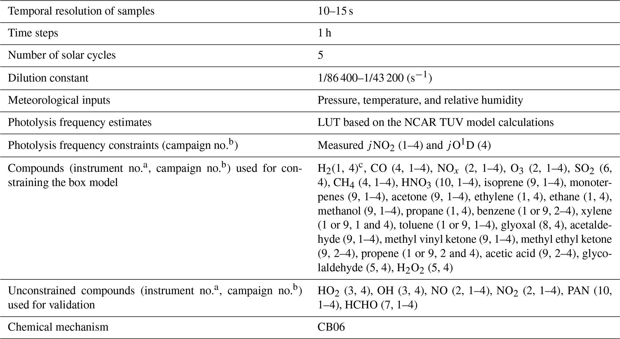
a (1) UC Irvine's Whole Air Sampler (WAS), (2) NCAR's 4-Channel Chemiluminescence, (3) Penn State's Airborne Tropospheric Hydrogen Oxides Sensor (ATHOS), (4) NASA Langley's DACOM tunable diode laser spectrometer, (5) Caltech's single mass analyzer, (6) Georgia Tech's ionization mass spectrometer, (7) the University of Colorado at Boulder's Compact Atmospheric Multi-species Spectrometer (CAMS), (8) Korean Airborne Cavity Enhanced Spectrometer, (9) University of Innsbruck's PTR-TOF-MS instrument, and (10) UC Berkeley's TD-LIF. b (1) DISCOVER-Baltimore-Washington, (2) DISCOVER-Texas-Houston, (3) DISCOVER-Colorado, and (4) KORUS-AQ. c In the absence of measurements, a default value of 550 ppbv is specified.
Figure 1 shows the map of data points from Deriving Information on Surface Conditions from Column and Vertically Resolved Observations Relevant to Air Quality (DISCOVER-AQ) Baltimore-Washington (2011), DISCOVER-AQ Houston-Texas (2013), DISCOVER-AQ Colorado (2014), and the Korea United States Air Quality Study (KORUS-AQ) (2016). Meteorological inputs come from the observed pressure, temperature, and relative humidity. The measurements of photolysis rates are not available for all photolysis reactions; therefore, our initial guess of those rates comes from a look-up table populated by the National Center for Atmospheric Research (NCAR) Tropospheric Ultraviolet And Visible (TUV) model calculations. These values are a function of solar zenith angle, total ozone column density, surface albedo, and altitude. We set the total ozone column and the surface albedo to fixed numbers of 325 DU (Dobson units) and 0.15, respectively. The initial guess is then corrected by applying the ratio of observed photolysis rates of NO2+hv (jNO2) and/or O3+hv (jO1D) to the calculated ones for all j values (i.e., wavelength-independent). If both observations of jNO2 and jO1D are available, the correction factor is averaged. The KORUS-AQ campaign is the only one that provides jO1D measurements; therefore, the use of the wavelength-independent correction factor based on the ratio of observed to calculated jNO2 values for all j values is a potential source of error in the model, especially when aerosols are present. The model calculations are based on the observations merged to a temporal resolution varying from 10 to 15 s. Each calculation was run for 5 consecutive days with an integration time of 1 h to approach the diel steady state. We test the number of solar cycles against 10 d on the KORUS-AQ setup and observe no noticeable difference in simulated OH and HCHO (Fig. S1 in the Supplement), indicating that five solar cycles suffice. Some secondarily formed species must be unconstrained for the purpose of model validation. Therefore, the concentrations of several secondarily formed compounds, such as HCHO and peroxyacetyl nitrate (PAN), are unconstrained. Nitric oxide (NO) and NO2 are also allowed to cycle, while their sum (i.e., NOx) is constrained. Because the model does not consider various physical loss pathways, including deposition and transport, which vary by time and space, we oversimplify their physical loss through a first-order dilution rate set to 400– 200 s−1 (i.e., 24 or 12 h lifetime), which in turn prevents relatively long-lived species from accumulating over time. Our decision on unconstraining HCHO, a pivotal compound impacting the simulation of HOx, may introduce some systematic biases into the simulation of radicals determining ozone chemistry (Schroeder et al., 2020). Therefore, to mitigate the potential bias in HCHO, we set the dilution factor to maintain the campaign-averaged bias in the simulated HCHO with respect to observations of less than 5 %. However, it is essential to recognize that HCHO can fluctuate freely for each point measurement because the dilution constraint is set to a fixed value for an individual campaign. Each time tag is independently simulated, meaning we do not initialize the next run using the simulated values from the previous one; this in turn permits parallel computation. Regarding the KORUS-AQ campaign where HOx observations were available, we only ran the model for data points with HOx measurements. Similarly to Souri et al. (2020), we filled gaps in VOC observations with a bilinear interpolation method with no extrapolation allowed. In complex polluted atmospheric conditions such as that over Seoul, South Korea, Souri et al. (2020) observed that this simple treatment yielded comparable results with respect to the NASA LaRC model (Schroeder et al., 2020), which incorporated a more comprehensive data harmonization. Table 1 lists the major configurations along with the observations used for the box model.
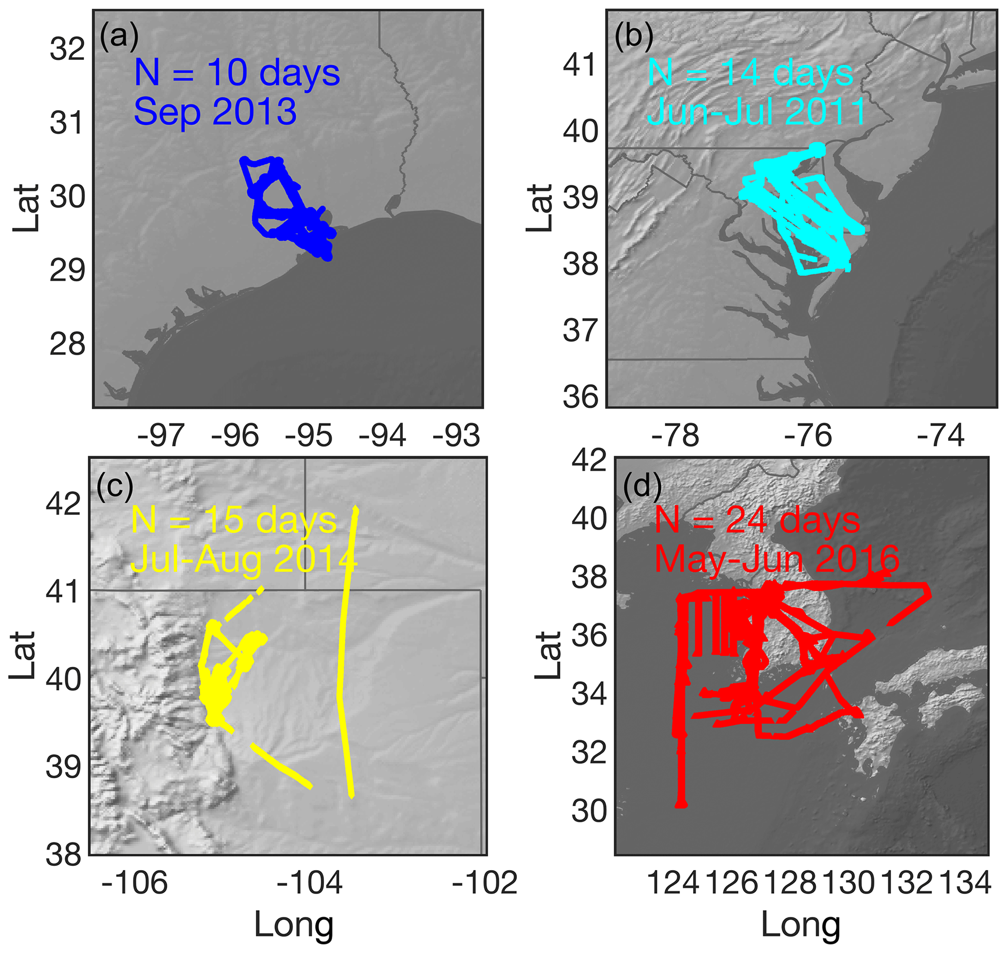
Figure 1The spatial distributions of aircraft measurements collected during NASA's (a) DISCOVER-AQ Houston-Texas, (b) DISCOVER-AQ Baltimore-Washington, (c) DISCOVER-AQ Colorado, and (d) KORUS-AQ. The duration of each campaign is based on how long the aircraft was in the air.
Several parameters are calculated based on the box model outputs. LROx is defined through the sum of primarily radical–radical reactions:
where k is the reaction rate constant. LNOx mainly occurs via the NO2+ OH reaction:
where M is a third body. We calculate P(O3) by subtracting the ozone loss pathways dictated by HOx (HO + HO2), NO2 + OH, O3 photolysis, ozonolysis, and the reaction of O(1D) with water vapor from the formation pathways through the removal of NO via HO2 and RO2:
3.1 Box model validation
There are uncertainties associated with the box model (e.g., Brune et al., 2022; Zhang et al., 2021; Lee et al., 2021), which can be attributed to (i) the lack of inclusion of physical processes such as entrainment/detrainment and diffusion, (ii) discounting the heterogeneous chemistry, (iii) invalid assumption of the diel steady state in areas close to large emission sources or in photochemically less active environments (Thornton et al., 2002; Souri et al., 2021), (iv) errors in the chemical mechanism, and (v) errors in the measurements. These limitations necessitate a thorough validation of the model using unconstrained observations. While models have been known for a long time not to be 100 % accurate (Box, 1976), it is important to characterize whether the model can effectively represent reality. For instance, if the simulated HCHO is poorly correlated with observations and/or displayed large magnitude biases, it will be erroneous to assume that the sources of HCHO, along with the relevant chemical pathways, are appropriate. It is important to acknowledge that the VOC constraints for these model calculations are incomplete, especially for the DISCOVER-AQ campaigns, which lacked comprehensive VOC observations. Nevertheless, we will show that the selected VOCs are sufficient to reproduce a large variance (> 70 %) in observed HCHO.
We diagnose the performance of the box model by comparing the simulated values of six compounds to observations: HCHO, NO, NO2, PAN, hydroperoxyl radical (HO2), and OH. Figure 2 depicts the scatterplot of the comparisons along with several statistics. HCHO observations are usually constrained in box models to improve the representation of HO2 (Schroeder et al., 2017; Souri et al., 2020; Brune et al., 2022); however, this constraint may mask the realistic characterization of the chemical mechanism with respect to the treatment of VOCs. Additionally, it is important to know whether the sources of HCHO are adequate. Therefore, we detach the model from this constraint to perform a fairer and more stringent validation.
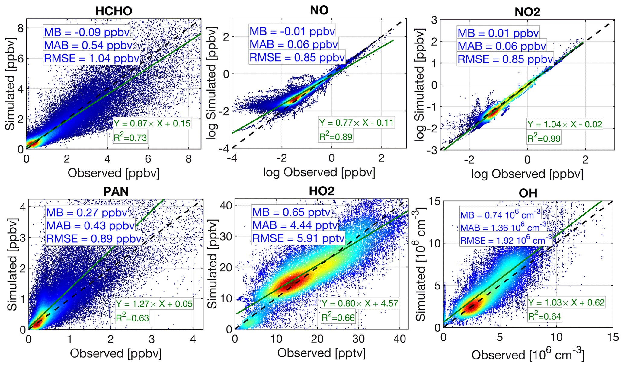
Figure 2The comparisons of the observed concentrations of several critical compounds to those simulated by our F0AM box model. Each subplot contains the mean bias (MB), mean absolute bias (MAB), and root mean square error (RMSE). The least-squares fit to the paired data and the coefficient of determination (R2) are also individually shown for each compound. Note that we do not account for the observation errors on the x axis. The concentrations of NO and NO2 are log-transformed.
Concerning HCHO, our model does have considerable skill in reproducing the variability of observed HCHO (R2=0.73). To evaluate whether this agreement is accidentally caused by the choice of the dilution factor and to identify whether our VOC treatment is inferior compared to the one adopted in the NASA LaRC (Schroeder et al., 2020), we conducted three sets of sensitivity tests for the KORUS-AQ campaign, including ones with and without considering a dilution factor and another one without HNO3 and H2O2 constraints (Fig. S2). The lack of consideration of a dilution factor results in no difference in the variance in HCHO captured by our model (R2=0.81). Our model without the dilution factor is still skillful in replicating the magnitude of HCHO with less than 12 % bias. This is why the optimal dilution factor for each campaign is within 12 to 24 h, which is not different from other box modeling studies (e.g., Brune et al., 2022; Miller and Brune, 2022). We observe no difference in the simulated HCHO when HNO3 and H2O2 values are not constrained. The unconstrained NASA LaRC setup oversampled at 10 s frequency captures 86 % variance in the measurements, only slightly (6 %) outperforming our result. However, the unconstrained NASA LaRC setup greatly underestimates the magnitude of HCHO compared to our model results.
The model performs well with regard to the simulation of NO (R2=0.89) and NO2 (R2=0.99) on the logarithmic scale. Immediately evident is the underestimation of NO in highly polluted regions, in contrast to an overestimation in clean ones. This discrepancy leads to an underestimation (overestimation) of in polluted (clean) regions. The primary drivers of are jNO2 and O3, both of which are constrained in the model. What can essentially deviate the partitioning between NO and NO2 from that of observations in polluted areas is the assumption of the diel steady state, which is rarely strictly valid where measurements are close to large emitters. The overestimation of NO in low-NOx areas is often blamed on the lack of chemical sink pathways of NO in chemical mechanisms (e.g., Newland et al., 2021). The relatively reasonable performance of PAN (R2=0.63) is possibly due to constraining some of the oxygenated VOCs, such as acetaldehyde. Xu et al. (2021) observed a strong dependency of PAN concentrations on ratios. Smaller ratios are usually associated with larger PAN mixing ratios because NO can effectively remove peroxyacetyl radicals. We observe an overestimated PAN (0.27 ppbv), possibly due to an underestimation of . Moreover, we should not rule out the impact of the first-order dilution factor, which was only empirically set in this study. For instance, if we ignore the dilution process for the KORUS-AQ campaign, the bias of the model in terms of PAN will increase by 33 %, resulting in poor performance (R2=0.40) (Fig. S3). We notice that this poor performance primarily occurs for high-altitude measurements where PAN is thermally stable (Fig. S4); therefore, this does not impact the majority of rapid atmospheric chemistry occurring in the lower troposphere, such as the formation of HCHO. Schroeder et al. (2020) found that proper simulation of PAN in the polluted PBL during KORUS-AQ required a first-order loss rate based on thermal decomposition at the average PBL temperature, which was more realistic than the widely varying local PAN lifetimes associated with temperature gradients between the surface and the top of the PBL. This solution is computationally equivalent to the dilution rate used in this study.
KORUS-AQ was the only field campaign providing OH and HO2 measurements. Concerning HO2, former studies such as Schroeder et al. (2017), Souri et al. (2020), and Brune et al. (2022) managed to reproduce HO2 mixing ratios with R2 ranging from 0.6 to 0.7. The performance of our model (R2=0.66) is similar to these past studies, with nearly negligible biases (< 1 %). One may argue that the absence of the HO2 uptake by aerosols is contributing to some of the discrepancies we observe in the HO2 comparison. Brune et al. (2022) provided compelling evidence showing that considering the HO2 uptake made their results significantly inconsistent with the observations, suggesting that the HO2 uptake might have been inconsequential during the campaign. Our model manages to reproduce 64 % of the variance of observed OH, outperforming the simulations presented in Souri et al. (2020) and Brune et al. (2022) by > 10 %. The slope (= 1.03) is not too far from the identity line, indicating that our box model systematically overestimates OH by 0.62×106 cm−3. This may be attributed to a missing OH sink in the mechanism or the lack of inclusion of some VOCs. A sensitivity test involving removing the first-order dilution process demonstrates that the simulation of HOx is rather insensitive to this parameter (Fig. S5). In general, the model performance is consistent, or outperforms, results from recent box modeling studies, indicating that it is at least roughly representative of the real-world ozone chemistry and sensitivity regimes.
3.2 Can HCHO NO2 ratios fully describe the HOx–ROx cycle?
Kleinman et al. (2001) demonstrated that is the most robust ozone regime indicator. Thus, the predictive power of FNRs in detecting the underlying chemical conditions can be challenged by comparing FNRs to . Ideally, if they show a strong degree of correspondence (i.e., R2=1.0), we can confidently say that FNRs can realistically portray the chemical regimes. Any divergence of these two quantities indicates the inadequacy of the FNR indicator. Souri et al. (2020) observed a strong linear relationship between the logarithmic-transformed FNRs and those of . Our analysis in this study will be based on the simulated values to ensure that the relationship is coherent based on a realization from the well-characterized box model. As pointed out by Schroeder et al. (2017) and Souri et al. (2020), a natural logarithm of roughly equal to −1.0 (i.e., = 0.35–0.37) perceptibly separates VOC-sensitive from NOx-sensitive regimes, which would make this threshold the baseline of our analysis.
Figure 3 demonstrates the log–log relationship of , FNRs, and P(O3) from all four air quality campaigns. The log–log relationships from each individual campaign are shown in Figs. S6–S9. We overlay the baseline threshold along with two commonly used thresholds for FNRs suggested by Duncan et al. (2010); they defined VOC-sensitive regimes if FNR < 1 and NOx-sensitive ones if FNR > 2. Any region undergoing a value between these thresholds is unlabeled and considered to be in a transitional regime. The size of each data point is proportional to the HCHO × NO2 concentration magnitude. One striking finding from this plot is that there is indeed a strong linear relationship between the logarithmic-transformed and the FNR (R2=0.91). A strong linear relationship between the two quantities in the log–log scale indicates a power law dependence (i.e., y=axb). A strong power law dependence means that these two quantities have a poor correlation at their low and high values. This is mainly caused by the fact that HCHO does not fully describe VOC reactivity rates in environments with high and low VOC concentrations (Souri et al., 2020). The question is what range of FNRs will fall in ln() = −1.0 ± 0.2. Following the baseline, the transitioning ratios follow a normal distribution with a mean of 1.8, a standard deviation of 0.4, and a range from 1 to 4 (Fig. S10). We define the chemical error in the application of FNRs to separate the chemical regimes as the relative error standard deviation (i.e., ) of the transitioning ratios leading to ∼ 20 %. These numbers are based on a single model realization and can change if a different mechanism is used; nonetheless, the model has considerable skill in reproducing many different unconstrained compounds, especially OH, suggesting that it is a rather reliable realization. Comparing the transitioning FNRs to the NO2 concentrations suggests no correlation (r=0.02), whereas there is a linear correlation between the transitioning ratios and the HCHO concentrations (r=0.56). This tendency reinforces the study of Souri et al. (2020), who, primarily due to the HCHO–NO2 feedback, observed a larger FNR threshold in VOC-rich environments to be able to detect the chemical regimes.
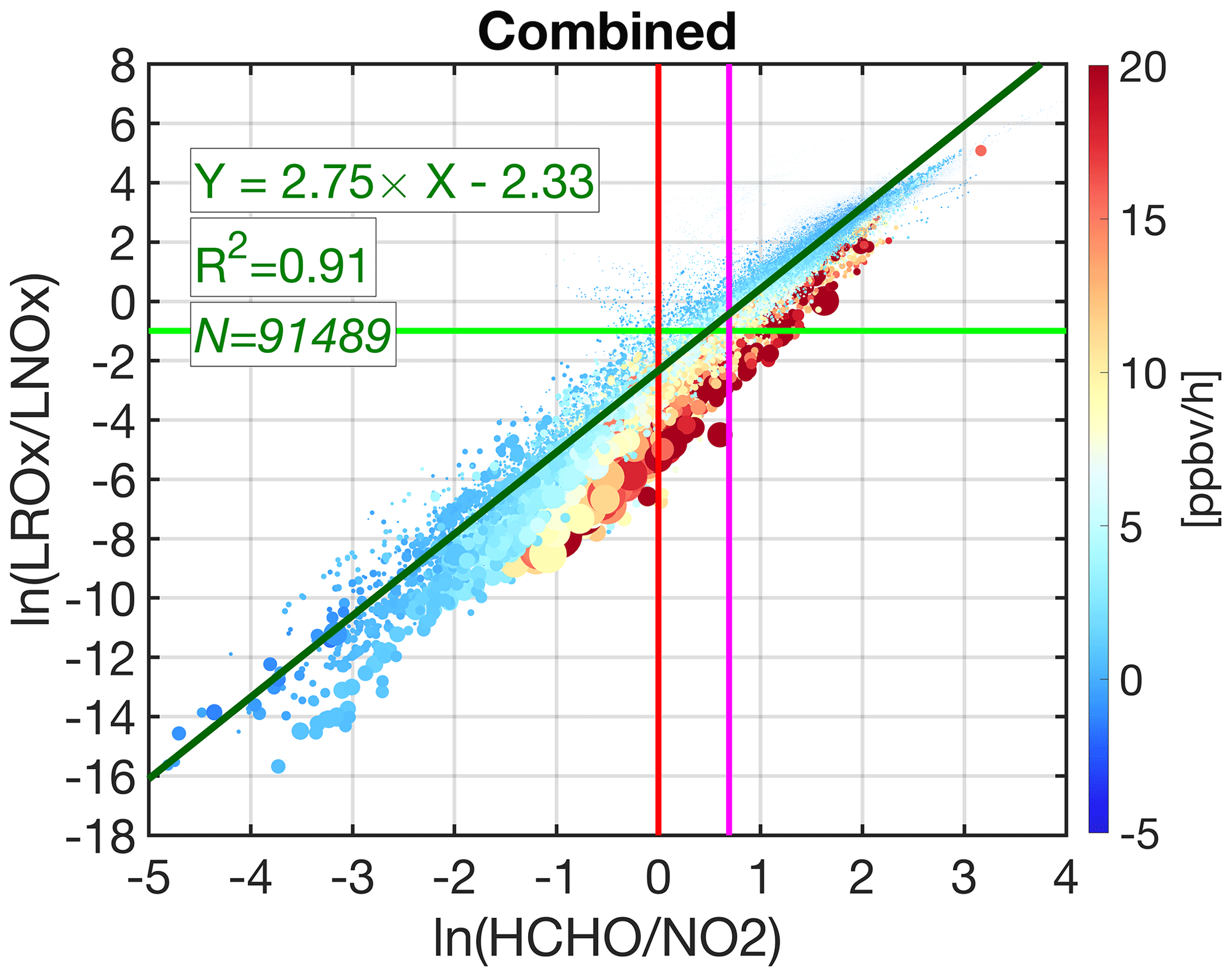
Figure 3The scatterplot of natural logarithm-transformed versus based on the simulated values performed by the F0AM box model. The heat color indicates the calculated ozone production rates (PO3). The size of each data point is proportional to HCHO × NO2. The black line is the baseline separator of NOx-sensitive (above the line) and VOC-sensitive (below the line) regimes. We overlay and as red and purple lines, respectively. The dashed dark green line indicates the least-squares fit to the paired data. The .8 with a 20 % error is the optimal transitioning point based on this result.
3.3 Large PO3 rates occur in regions with large HCHO × NO2 concentrations when moving towards NOx-sensitive regions
A striking and perhaps intuitive tendency observed from Fig. 3 is that large PO3 rates are mostly tied to higher HCHO × NO2. However, this relationship gradually weakens as we move towards VOC-sensitive regions (smaller ratios). This is a textbook example of nonlinear ozone chemistry. In VOC-sensitive areas, PO3 can be strongly inhibited by NO2+ OH and the formation of organic nitrates despite the abundance of the precursors. In the application of remote sensing of ozone precursors, the greatest unused metric describing the mass of the ozone precursors is HCHO × NO2. However, this metric should only be used in conjunction with FNRs. To demonstrate this, based on what the baseline () suggests against thresholds on FNRs defined by Duncan et al. (2010), we group the data into four regions: NOx-sensitive–NOx-sensitive, NOx-sensitive–transitional, VOC-sensitive–transitional, and VOC-sensitive–VOC-sensitive. A different perspective on this categorization is that the transitional regimes are a weaker characterization of the main regime; for instance, NOx-sensitive–transitional regions are less NOx-sensitive than NOx-sensitive–NOx-sensitive. Subsequently, the cumulative distribution functions (CDFs) of PO3 and HCHO × NO2 with respect to the aforementioned groups are calculated, which is shown in Fig. 4. Regarding NOx-sensitive–NOx-sensitive regions, we see the PO3 CDF very quickly converging to the probability of 100 %, indicating that the distribution of PO3 is skewed towards very low values. The median of PO3 for this particular regime (where CDF = 50 %) is only 0.25 ppbv h−1. This agrees with previous studies such as Martin et al. (2002), Choi et al. (2012), Jin et al. (2017), and Souri et al. (2017) reporting that NOx-sensitive regimes dominate in pristine areas. The PO3 CDFs between NOx-sensitive–transitional and VOC-sensitive–VOC-sensitive are not too distinct, whereas their HCHO × NO2 CDFs are substantially different. The nonlinear ozone chemistry suppresses PO3 in highly VOC-sensitive areas such that those values are not too different from those in mildly polluted areas (NOx-sensitive–transitional). Perhaps the most interesting conclusion from this figure is that elevated PO3 values (median = 4.6 ppbv h−1), a factor of 2 larger than two previous regimes, are mostly found in VOC-sensitive–transitional. This is primarily due to two causes: (i) this particular regime is not strongly inhibited by the nonlinear chemistry, particularly NO2+ OH, and (ii) it is associated with abundant precursors evident in the median of HCHO × NO2 being 3 times as large of those in NOx-sensitive–transitional. This tendency illustrates the notion of nonlinear chemistry and how this may affect regulations. Simply knowing where the regimes are might not suffice to pinpoint the peak of PO3, as this analysis suggests that we need to consider both the FNR and HCHO × NO2; both metrics are readily accessible from satellite remote-sensing sensors.
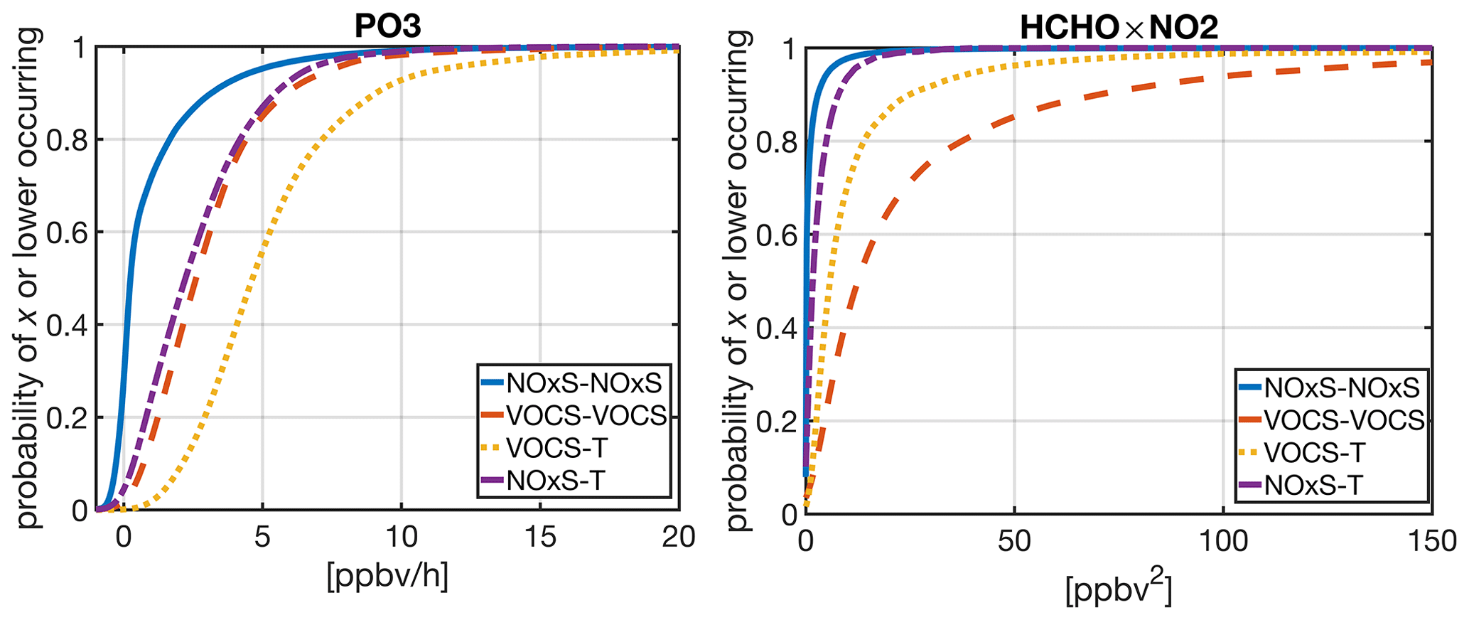
Figure 4Cumulative distribution functions of PO3 and HCHO × NO2 simulated by the box model constrained by NASA's aircraft observations. Four regions are shown: NOx-sensitive–NOx-sensitive, NOx-sensitive–transitional, VOC-sensitive–transitional, and VOC-sensitive–VOC-sensitive. The first name of the regime is based on the baseline (ln() .0), whereas the second one follows those defined in Duncan et al. (2010): VOC-sensitive if < 1, transitional if 1 < < 2, and NOx-sensitive if > 2.
3.4 Can we estimate PO3 using the information from HCHO NO2 and HCHO × NO2?
It may be advantageous to construct an empirical function fitted to these two quantities and elucidate the maximum variance (information) we can potentially gain to recreate PO3. After several attempts, we found a bilinear function () to be a good fit without overparameterization. Due to the presence of extreme values in both the FNR and HCHO × NO2, we use a weighted least-squares method for the curve fitting based on the distance of the fitted curve to the data points (known as bi-squares weighting). The best fit with R2 equals 0.94, and an RMSE of 0.60 ppbv h−1 is
where x and y are the FNR (unitless) and HCHO × NO2 (ppbv2), respectively. The residual of the fit is shown in Fig. S11. The gradients of PO3 with respect to x and y are
An apparent observation arises from these equations: i.e., the derivative of PO3 to each metric depends on the other one underscoring their interconnectedness. For instance, Eq. (6) suggests that larger FNRs (x) result in a larger gradient of PO3 to the abundance of HCHO × NO2(y). In very low FNRs, this gradient can become very small, rendering PO3 insensitive to (or in extreme cases, negatively correlated with) HCHO × NO2. This analysis provides encouraging results about the future application of the satellite-derived HCHO × NO2; however, the wide class of problems relating to the application of satellite-derived FNR columns, such as satellite errors in columns or the translation between columns to the PBL, is also present in Eq. (4), even in a more pronounced way due to HCHO × NO2 and HCHO2 (=xy). This new perspective on PO3 estimation deserves a separate study.
3.5 Altitude dependency and its parametrization
A lingering concern over the application of satellite-based FNR tropospheric columns is that the vertical distributions of HCHO and NO2 are integrated into columns; thus, this vertical information is permanently lost. Here, we provide insights into the vertical distribution of FNRs within the tropospheric column. This task requires information about the differences between (i) the vertical shape of HCHO and that of NO2 and (ii) the vertical shape in the sensitivity of the retrievals to the different altitude layers (described as scattering weights). Ideally, if both compounds show an identical relative shape, the FNR columns will be valid for every air parcel along the vertical path (i.e., a straight line). Previous studies such as Jin et al. (2017) and Schroeder et al. (2017) observed a large degree of vertical inhomogeneity in both HCHO and NO2 concentrations, suggesting that this ideal condition cannot be met. We do not always have precise observations of HCHO and NO2 vertical distributions, but we can constitute some degree of generalization by leveraging the measurements made during the aircraft campaigns. As for the differences in the vertical shapes (i.e., the curvature) of the sensitivity of the retrievals between HCHO and NO2 channels (i.e., ∼ 340 and ∼ 440 nm), under normal atmospheric and viewing geometry conditions, several studies such as Nowlan et al. (2018) and Lorente et al. (2017) showed small differences in the vertical shapes of the scattering weights in the first few kilometers in altitude above the surface, where the significant fluctuations in FNRs usually take place. Therefore, our analysis does not consider the varying vertical shapes in the scattering weights. However, this assumption might not hold for excessive aerosol loading with variable extinction efficiency between ∼ 340 and ∼ 440 nm wavelengths or extreme solar zenith angles.
Figure 5 demonstrates the violin plot of the afternoon (> 12:00 LT) vertical distribution of HCHO, NO2, and FNRs observed by NASA's aircraft during the four field campaigns analyzed in this study superimposed by the simulated PO3 rates. The vertical layers are grouped into 16 altitudes ranging from 0.25 to 7.75 km. Each vertical layer incorporates measurements ±0.25 km of the mid-layer height. The observations do not follow a normal distribution, particularly in the lower parts of the atmosphere; thus, medians are preferred to represent the central tendency. While the largest PO3 rates tend to occur in areas close to the surface (< 2 km a.g.l.), non-negligible fractions of the elevated PO3 rates are also observed in other parts of the atmosphere, such as in the free troposphere.
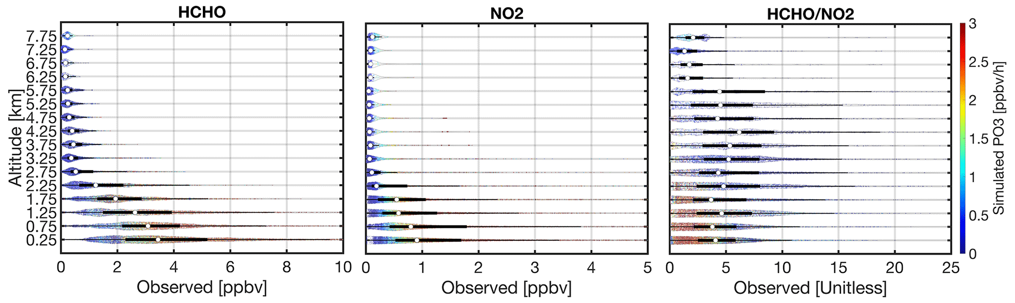
Figure 5The violin plots of the afternoon vertical distribution of HCHO, NO2, and observations collected during the DISCOVER-AQ Texas, Colorado, Maryland, and KORUS-AQ campaigns. The violin plots demonstrate the distribution of data (i.e., a wider width means a higher frequency). White dots show the median. A solid black line shows both the 25th and 75th percentiles. The heatmap denotes the simulated ozone production rates.
Several intriguing features are observed in Fig. 5. First, up to the 5.75 km range, which encompasses the PBL area and a large portion of the free troposphere, NO2 concentrations tend to decrease more quickly than those of HCHO, in line with previous studies such as Schroeder et al. (2017), Jin et al. (2017), Chan et al. (2019), and Ren et al. (2022). Second, above 5.75 km, HCHO levels off, whereas NO2 shows an increasing trend. Finally, due to their different vertical shapes, we observe non-uniformities in the vertical distribution of FNRs: they become more NOx-sensitive with altitude up to a turning point at 5.75 km and then shift back to the VOC-sensitive direction.
It is attractive to model these shapes and apply parameterizations to understand how their shapes will complicate the use of tropospheric column retrieval from satellites. First-order rational functions are a good candidate to use. Concerning the vertical dependency of HCHO and NO2, we find a reasonable fit (R2=0.73) as
where z is altitude in kilometers. ai () are fitting parameters. From this equation it is determined that FNRs follow a second-order rational function:
where bi () are fitting parameters. One can effortlessly fit this function to different bounds of the vertical distribution of FNRs such as the 25th and 75th percentiles and subsequently estimate the first moment of the resultant polygon along z divided by the total area bounded to the polygon (the centroid G) via
where A is the area of the polygon bounded by the 75th percentiles, f(z)75th, and 25th percentiles (f(z)25th) of FNRs (shown in Fig. 5 as solid black lines). We define an altitude adjustment factor (fadj) such that one can translate observed FNR tropospheric column ratios, such as those retrieved from satellites, to a defined altitude and below that point (zt) through
where zt can be interchanged to match the planetary boundary layer height (PBLH). This definition is more beneficial than using the entire tropospheric column to surface conversion (e.g., Jin et al., 2017) because ozone can form in various vertical layers. Using the observations collected during the campaign, we estimate Eq. (10) along with ±1σ boundaries shown in Fig. 6. To determine the adjustment factor error, we reestimate Eq. (9) with the ±1σ level in the coefficients obtained from Eq. (8). The resultant error is shown in the dashed red line in Fig. 6. This error results from uncertainties associated with assuming that the second-order rational function can explain the vertical distribution of FNRs. The shape of the resulting adjustment factor is in line with the vertical distribution of FNRs (see Fig. 5): the adjustment factor curve closer to the surface has values smaller than 1, increases to values larger than 1 in the mid-troposphere, and finally converges to 1 near the top of measured concentrations. If one picks out an altitude pertaining to a PBLH, one can easily apply fadj to the observed FNR columns to estimate the corresponding ratio for that specific PBLH. A more evolved PBLH (i.e., a large zt) results in stronger vertical mixing, rendering fadj closer to 1. The standard error deviation of this conversion is around 19 %. The relatively low fluctuations in the adjustment factor around 1 suggest that under the observed atmospheric conditions (clear-sky afternoon summers), the columnar tropospheric ratios do not poorly represent the chemical conditions in the PBL region.

Figure 6The adjustment factor is the ratio of the centroid of the polygon-bounding 25th and 75th percentiles of the observed columns by NASA's aircraft between the surface and 8 km to the ones between the surface and the desired altitude. This factor can be easily applied to the observed columns to translate the value to the desired altitude stretching down to the surface (i.e., PBLH). The optimal curve follows a quadratic function formulated in Eq. (11).
It is beneficial to model this curve to make this data-driven conversion easier for future applications. A second-order polynomial can well describe (R2=0.97) this curve:
Although Eq. (11) does not include observations above 8 km, the area bounded between f(z)75th and f(z)25th at higher altitudes is too small to make a noticeable impact on this adjustment factor.
One may object that since we estimated the adjustment factor based on two boundaries (25th and 75th percentiles) of the data, we are no longer really dealing with 50 % of features observed in the vertical shapes of FNRs. This valid critique can be overcome by gradually relaxing the lower and upper limits and examining the resulting change in fadj. When we reduce the lower limit in Eq. (9) from the 25th to 1st percentiles, the optimal curve is similar to the one shown in Fig. 6 (Fig. S12). However, when we extend the upper limit from the 75th percentile to greater values, we see the fit becoming less robust above the 80th percentile, indicating that the formulation applies to ∼ 80 % of the data. The reason behind the poor representation of the adjustment factor for the upper tail of the population is the extremely steep turning point between 5.5 and 6.0 km, necessitating a higher-order rational function to be used for Eqs. (7) and (8). We prefer to limit this analysis to both boundaries and the order defined in Eqs. (8) and (9) because extreme value predictions usually lack robustness.
A caveat with these results is that our analysis is limited to afternoon observations because we focus on afternoon low-orbiting sensors such as OMI and TROPOMI. Nonetheless, Schroeder et al. (2017) and Crawford et al. (2021) observed large diurnal variability in these profiles due to diurnal variability in sinks and sources of NO2 and HCHO and atmospheric dynamics. The diurnal cycle has an important implication for geostationary satellites such as Tropospheric Emissions indeed: Monitoring of Pollution (TEMPO) (Chance et al., 2019). Limiting the observations to morning time results in a smaller adjustment factor for altitudes close to the surface resulting from steeper vertical gradients of (Figs. S13 and S14). This tendency agrees with Jin et al. (2017), who observed a larger deviation from 1 in an adjustment factor used for the column–surface conversion in winter.
Another important caveat with our analysis is that it is based upon four air quality campaigns in warm seasons that avoid times/areas with convective transport; as such, our analysis needs to be made aware of the vertical shapes of FNRs during convective activities and cold seasons. However, a few compelling assumptions can minimize these oversights: first, it is very atypical to encounter elevated ozone production rates during cold seasons, with few exceptions (Ahmadov et al., 2015; Rappenglück et al., 2014); second, the notion of ozone regimes is only appropriate in photochemically active environments where the ROx–HOx cycle is active. An example of this can be found in Souri et al. (2021), who observed an enhancement of surface ozone in central Europe during a lockdown in April 2020 (up to 5 ppbv) compared to a baseline which was explainable by the reduced O3 titration through NO in place of the photochemically induced production. An exaggerated extension to this example is the nighttime chemistry where NO–O3–NO2 partitioning is the primary driver of negative ozone production rates; at night, the definition of NOx-sensitive or VOC-sensitive is meaningless, so it is in photochemically less active environments. Third, it is rarely advisable to use cloudy scenes in satellite UV–Vis gas retrievals due to the arguable assumption about Lambertian clouds and a highly uncertain cloud optical centroid and albedo. Accordingly, atmospheric convection occurring during storms or fires is commonly masked in satellite-based studies. Therefore, the limitations associated with the adjustment factor are mild compared to the advantages.
3.6 Spatial heterogeneity
The spatial representation error resulting from unresolved processes and scales (Janjić et al., 2018; Valin et al., 2011; Souri et al., 2022) refers to the amount of information lost due to satellite footprint or unresolved inputs used in satellite retrieval algorithms. Unfortunately, this source of error cannot be determined when we do not know the true state of the spatial variability. There is, however, a practical way of resolving this by conducting multi-scale intercomparisons of a coarse spatial resolution output against a finer one. Yet despite the absence of the truth in this approach, we tend to find their comparisons useful in giving us an appreciation of the error.
We build the reference data on qualified pixels (qa_value > 0.75) of the offline TROPOMI tropospheric NO2 version 2.2.0 (van Geffen et al., 2022; Boersma et al., 2018) and total HCHO columns version 2.02.01 (De Smedt et al., 2018) oversampled at 3 × 3 km2 in summer 2021 over the US. Figure 7 shows the map of those tropospheric columns as well as FNRs. Encouragingly, the small footprint and relatively low detection limit of TROPOMI compared to its predecessor satellite sensors (e.g., OMI) enable us to have possibly one of the finest maps of HCHO over the US to date. Large values of HCHO columns are found in the southeast due to strong isoprene emissions (e.g., Zhu et al., 2016; Wells et al., 2020). Cities like Houston (Boeke et al., 2011; Zhu et al., 2014; Pan et al., 2015; Diao et al., 2016), Kansas City, Phoenix (Nunnermacker et al., 2004), and Los Angeles (de Gouw et al., 2018) also show pronounced enhancements of HCHO possibly due to anthropogenic sources. Expectedly, large tropospheric NO2 columns are often confined to cities and some coal-fired power plants along the Ohio River basin. Concerning FNRs, low values dominate cities, whereas high values are found in remote regions. An immediate tendency observed from these maps is that the length scale of HCHO columns is longer than that of NO2. This indicates that NO2 columns are more heterogeneous. Because of this, we observe a large degree of spatial heterogeneity with respect to FNRs.

Figure 7Oversampled TROPOMI total HCHO columns (a), tropospheric NO2 columns (b), and the ratio (c) at 3 × 3 km2 from June till August 2021 over the US. The ratio map is derived from the averaged maps shown in panels (a) and (b).
Here we limit our analysis to Los Angeles due to computational costs imposed by the subsequent experiment. To quantify the spatial representation errors caused by satellite footprint size, we upscale the FNRs by convolving the values with four low-pass box filters with sizes of 13 × 24, 36 × 36, 108 × 108, and 216 × 216 km2, shown in the first column of Fig. 8. Subsequently, to extract the spatial variance (information), we follow the definition of the experimental semivariogram (Matheron, 1963):
where Z(xi) and Z(xj) are discrete pixels of FNRs, and N(h) is the number of paired pixels separated by the vector of h. The operator indicates the length of a vector. The condition of is to permit a certain tolerance for differences in the length of the vector. Here, we ignore the directional dependence in γ(h) which makes the vector of h a scalar (). Moreover, we bin γ values in 100 evenly spaced intervals ranging from 0 to 5∘. To remove potential outliers (such as noise), it is wise to model the semivariogram using an empirical regression model. To model the semivariogram, we follow the stable Gaussian function used by Souri et al. (2022):
where r and s are fitting parameters. For the most part, geophysical quantities become spatially uncorrelated at a certain distance called the range, and the variance associated with that distance is called the sill. The fitting parameters, r, and s, describe these two quantities as long as the stable Gaussian function can well fit the shape of a semivariogram. The semivariograms and the fits associated with each map are depicted in the second column of Fig. 8.
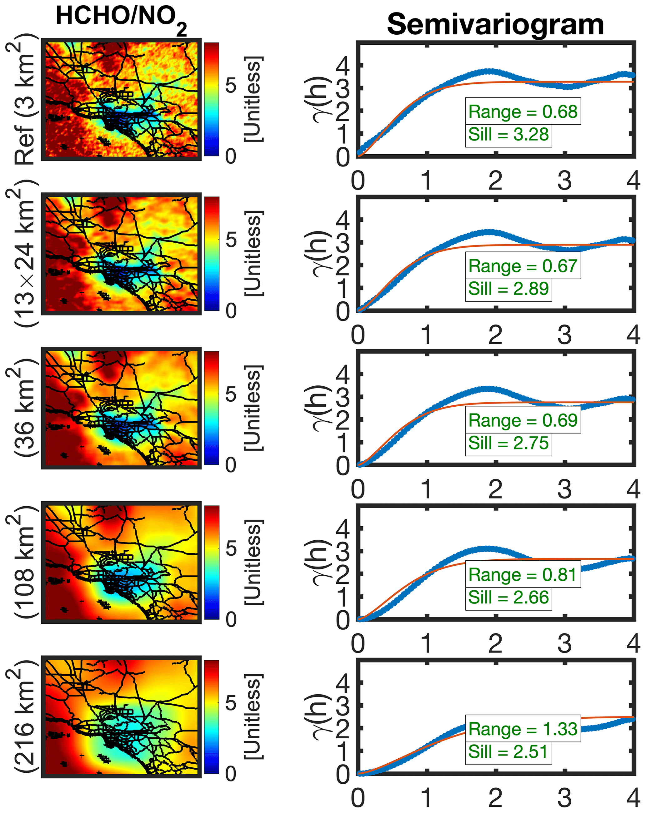
Figure 8The first column represents the spatial map of ratios over Los Angeles from June till August 2021 at different spatial resolutions. To upscale each map to a coarser footprint, we use an ideal box filter tailored to the target resolution. The second column shows the semivariograms corresponding to the left map along with the fitted curve (red line). The sill and the range are computed based on the fitted curve. The x axis in the semivariogram is in degrees (1∘ ∼ 110 km).
The modeled semivariograms suggest that a coarser field comes with a smaller sill, implying a loss in the spatial information (variance). The length scale (i.e., the range) only sharply increases at coarser footprints (> 36 × 36 km2). This indicates that several coarse-resolution satellite sensors, such as OMI (13 × 24 km2), are rather able to determine the length scales of FNRs over a major city such as Los Angeles. By leveraging the modeled semivariograms, we can effortlessly determine the spatial representation error for a specific scale (e.g., h=10 km) through
where γ(h) and γref(h) are the modeled semivariogram of the target and the reference fields (3 × 3 km2). This equation articulates the amount of information lost in the target field compared to the reference. Accordingly, the proposed formulation of the spatial representation error is relative. Figure 9 depicts the representation errors for various footprints. For the most part, the OMI nadir pixel (13 × 24 km2) only has a ∼ 12 % loss of spatial variance. By contrast, a grid box with a size of 216 × 216 km2 fails at capturing ∼ 65 % of the spatial information in FNRs with a 50 km length scale comparable to the extent of Los Angeles. The advantage of our method is that we can mathematically describe the spatial representation error as a function of the length of our target. The present method can be easily applied to other atmospheric compounds and locations. We have named this method the SpaTial Representation Error EstimaTor (STREET), which is publicly available as an open-source package (Souri, 2022).
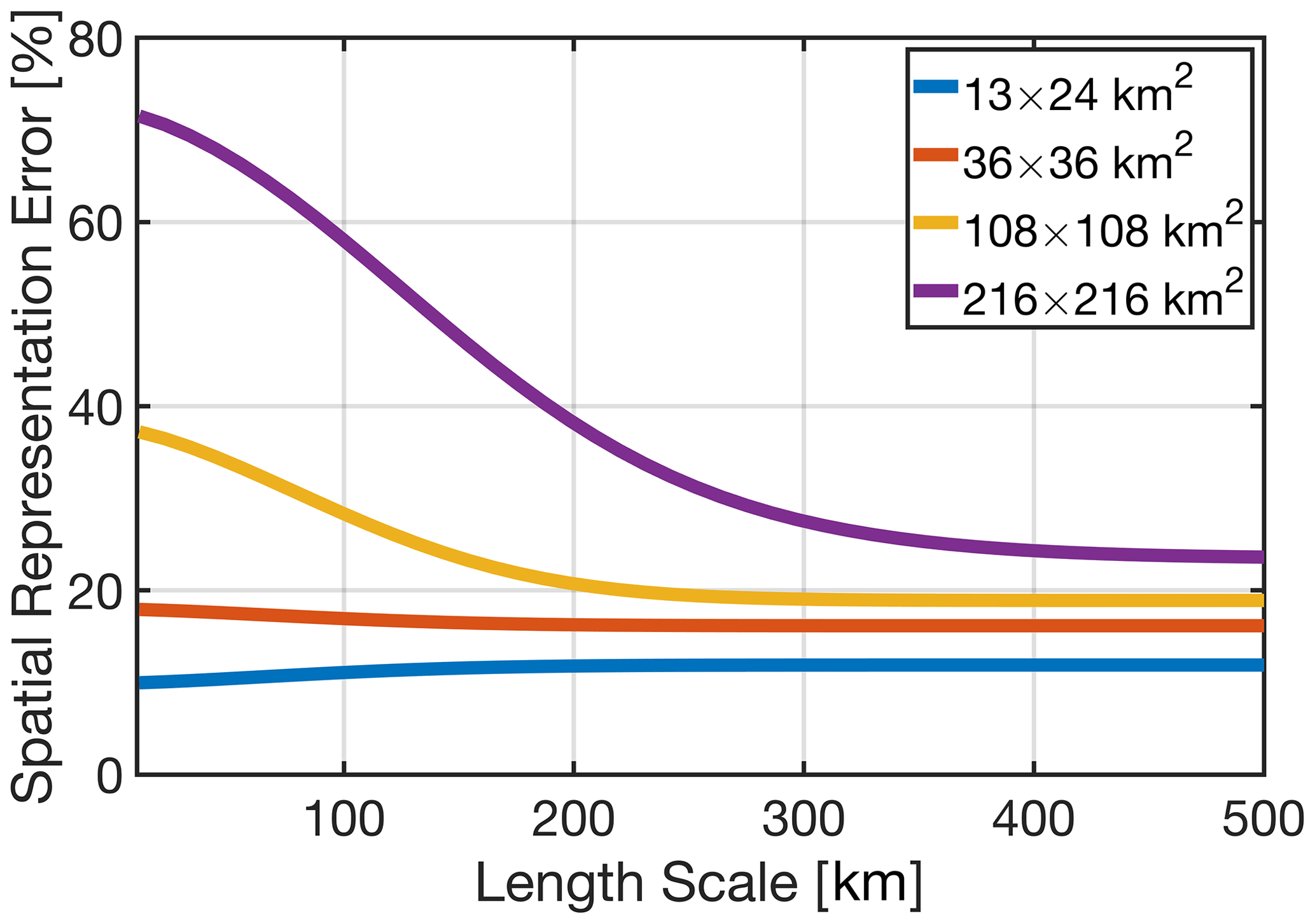
Figure 9The spatial representation errors quantified based on the proposed method in this study. The error explains the spatial loss (or variance) due to the footprint of a hypothetical sensor at different length scales. To put this error into perspective, a grid box with 216 × 216 km2 will naturally lose 65 % of the spatial variance existing in the ratio at the scale of Los Angeles, which is roughly 50 km wide. All of these numbers are in reference to the TROPOMI 3 × 3 km2.
An oversight in the above experiment lies in its lack of appreciation of unresolved physical processes in the satellite measurements: a weak sensitivity of some retrievals to the near-surface pollution due to the choice of spectral windows used for fitting (Yang et al., 2014), using 1-D air mass factor calculation instead of 3-D (Schwaerzel et al., 2020), and neglecting the aerosol effect on the light path are just a few examples to point out. To account for the unresolved processes, one can recalculate Eqs. (12)–(14) using outputs from different retrieval frameworks, which is beyond the scope of this study.
3.7 Satellite errors
3.7.1 Concept
Two types of retrieval errors can affect our analysis: systematic errors (bias) and unsystematic ones (random errors). In theory, it is very compelling to understand their differences. In reality, the distinction between random and systematic errors is not as clear-cut as it seems. For example, one may wish to establish the credibility of a satellite retrieval by comparing it to a sky-radiance measurement over time. Because each measurement is made at a different time, their comparison is not a repetition of the same experiment; each time, the atmosphere differs in some aspects, so each comparison is unique. Adding more sky-radiance measurements will add new experiments. For each paired data point, many unique issues contribute differently to errors; as such, our problem is grossly underdetermined (i.e., more unknowns for a given observation). Here, we do not attempt to separate random from systematic errors in the subsequent analysis, thereby limiting this study to the total uncertainty.
We focus on analyzing the statistical errors drawn from the differences between the benchmark and the retrievals on a daily basis. Two sensors are used for this analysis: TROPOMI and OMI. To propagate individual uncertainties in HCHO and NO2 to FNRs, we follow an analytical approach involving Jacobians of the ratio to HCHO and NO2. Assuming that errors in HCHO and NO2 are uncorrelated, the relative error of the ratio can be estimated by
where σHCHO and are total uncertainties of HCHO and NO2 observations. It is important to recognize that the errors in HCHO and NO2 are not strictly uncorrelated due to assumptions made in their air mass factor calculations.
3.7.2 Error distributions in TROPOMI and OMI
We begin our analysis with the error distribution of daily TROPOMI tropospheric NO2 columns (v1.02.02) against 22 MAX-DOAS instruments from May to September in 2018–2021. The data are paired based on the criteria defined in Verhoelst et al. (2021). The spatial locations of the stations are mapped in Fig. S15. Figure 10a shows the histogram of the TROPOMI minus MAX-DOAS instruments. The first observation from this distribution is that it is skewed towards lower differences, evident in the skewness parameter around −4.6. As a result of the skewness, the median should better represent the central tendency, which is around −1 × 10¹⁵ molec. cm−2. In general, TROPOMI tropospheric NO2 columns show a low bias. We fit a normal distribution to the data using the nonlinear Levenberg–Marquardt method. This fitted normal distribution (R2=0.94) is used to approximate for different confidence intervals and to minimize blunders. To understand how many of these disagreements are caused by systematic errors as opposed to random errors, we redo the histogram using monthly-based observations (Fig. S16). A slight change in the dispersions between the daily and monthly-basis analyses indicates the significance of unresolved systematic (or relative) biases. This tendency suggests that when conducting the analysis on a monthly basis, the relative bias cannot be mitigated by averaging. Verhoelst et al. (2021) rigorously studied the potential root cause of some discrepancies between MAX-DOAS and TROPOMI. An important source of error stems from the fundamental differences in the vertical sensitivities of MAX-DOAS (more sensitive to the lower-tropospheric region) and TROPOMI (more sensitive to the upper-tropospheric area). This systematic error can only be mitigated using reliably high-resolution vertical shape factors instead of spatiotemporal averaging of the satellite data.
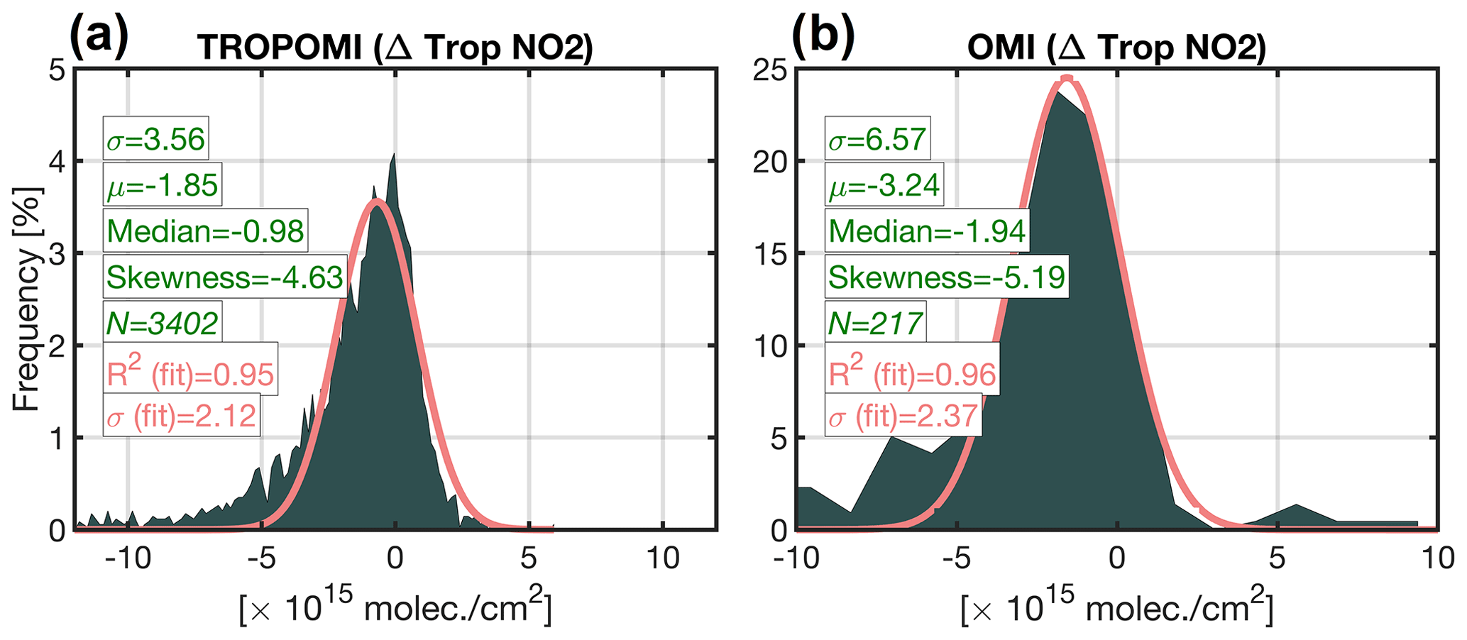
Figure 10The histogram of the differences between TROPOMI and OMI and benchmarks. MAX-DOAS and integrated aircraft spirals are the TROPOMI and OMI benchmarks, respectively. The data curation and relevant criteria on how they have been paired can be found in Verholest et al. (2021) and Choi et al. (2020). The statistics in green are based on all data, whereas those in pink are based on the fitted Gaussian function.
The error analysis for OMI follows the same methods applied for TROPOMI, however with different benchmarks. We follow the comparisons made between the operational product version 3.1 and measured columns derived from NCAR's NO2 measurements integrated along aircraft spirals during four NASA air quality campaigns. More information regarding this data comparison can be found in Choi et al. (2020). Figure 10b shows the histogram of OMI minus the integrated spirals. Compared to TROPOMI, the OMI bias is worse by a factor of 2. The standard deviation calculated from a Gaussian fit (2.31 × 10¹⁵ molec. cm−2) is not substantially different from that of TROPOMI (2.11 × 10¹⁵ molec. cm−2).
As for the error distribution of TROPOMI HCHO columns, version 1.1.(5–7), we use 24 FTIR measurements during the same time period based on the criteria specified in Vigouroux et al. (2020). The stations are mapped in Fig. S15. The frequency of the paired data is daily. Figure 11a depicts the error distribution. The distribution is slightly broader compared to that of NO2, manifested in a larger standard deviation of 4.32 × 10¹⁵ molec. cm−2. This is primarily due to two facts: (i) HCHO optical depths generally peak in the UV range (< 380 nm), where the large optical depths of ozone and Rayleigh scattering result in weaker and noisier signals (González Abad et al., 2019), and (ii) the broader and stronger NO2 optical depths in the Vis range (400–500 nm), where the signal-to-noise ratio is typically more outstanding, permitting better-quality retrievals. Similarly to the NO2, we fit a normal distribution (R2=0.90) to specify σHCHO for different confidence intervals.
Concerning OMI HCHO columns from SAO version 3 (González Abad et al., 2015), we follow the intercomparison approach proposed in Zhu et al. (2020). Based on this approach, the benchmarks come from GEOS-Chem-simulated HCHO columns corrected by in situ aircraft measurements. The measurements were made during ozone seasons from the KORUS-AQ, DISCOVERs, FRAPPE, NOMADSS, and SENEX campaigns (see Table 1 in Zhu et al., 2020). OMI values ranging from −0.5 × 10¹⁵ to 1.0 × 10¹⁷ molec. cm−2 with an effective cloud fraction between 0.0 and 0.3 and solar zenith angle between 0 and 60∘ are only considered in the comparison. Any pixels from OMI and grid boxes from the corrected GEOS-Chem simulation that fall into a polygon enclosing the campaign domain are used to create the error distribution shown in Fig. 11b. The distribution has much denser data because the model output covers a large portion of the satellite swath. The error distribution suggests that OMI HCHO is inferior to TROPOMI, evident in the larger bias and standard deviation. The OMI bias is twice as large as that of TROPOMI. De Smedt et al. (2021) observed the same level of bias from their comparisons of OMI/TROPOMI with MAX-DOAS instruments (see Table 3 in their paper). Moreover, their OMI versus MAX-DOAS comparisons were severely scattered. Likewise, we observe the standard deviation of OMI from the fitted Gaussian function to be roughly 5 times as large as that of TROPOMI. This can be primarily due to a weaker signal-to-noise ratio (and sensor degradation) in OMI. It is for this reason that OMI HCHO should be averaged over several months. Another possible reason for the large standard deviation is the fact that the benchmark arises from a modeling experiment whose ability to resolve spatiotemporal variations in HCHO may be uncertain. This partly leads to the performance of OMI looking poor.

Figure 11The histogram of the differences between TROPOMI and OMI and benchmarks. FTIR and corrected GEOS-Chem simulations are the TROPOMI and OMI benchmarks. The data curation and relevant criteria on how they have been paired can be found in Vigouroux et al. (2021) and Zhu et al. (2020). The statistics in green color are based on all data, whereas those in pink are based on the fitted Gaussian function.
3.7.3 The impact of retrieval error on the ratio
Following Eq. (15), we calculate the standard error for a wide range of NO2 and HCHO columns at a 68 % confidence interval (1σ) for both TROPOMI and OMI derived from the fitted Gaussian function to the histograms; the standard errors are shown in Fig. 12. We observe smaller errors to be associated with larger tropospheric column concentrations. As for TROPOMI, either daily HCHO or tropospheric NO2 columns should be above 1.2–1.5 × 10¹⁶ molec. cm−2 to achieve 20 %–30 % standard error. The TROPOMI errors start diminishing the application of FNRs when both measurements are below this threshold. Regarding OMI, it is nearly impossible to get the standard error below 20 %–30 % given its problematically large HCHO standard deviation. For 50 % error, the daily HCHO columns should be above 3.2 × 10¹⁶ molec. cm−2. This range of error can also be achieved if OMI tropospheric NO2 columns are above 8 × 10¹⁵ molec. cm−2.
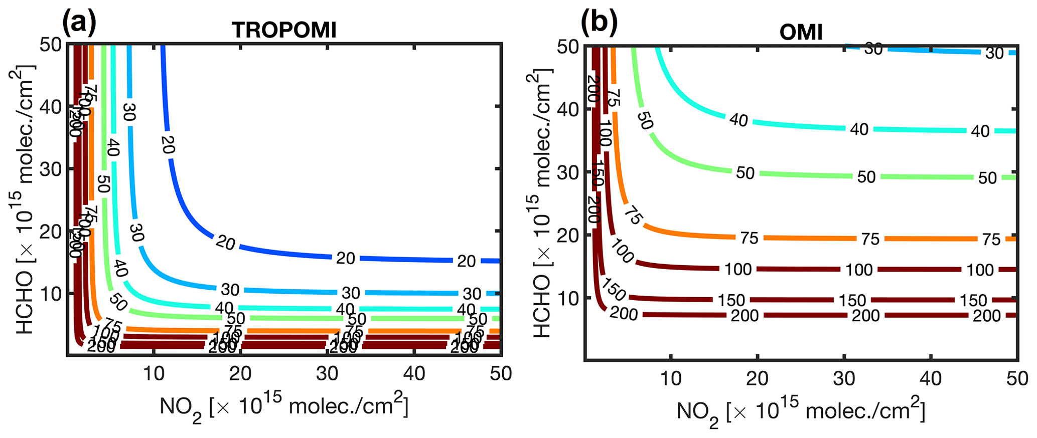
Figure 12The contour plots of the relative errors in TROPOMI (a) and OMI (b) based on dispersions derived from Figs. 10 and 11. The errors used for these estimates are based on daily observations.
3.8 The fractional errors to the combined error
The ultimate task is to compile the aforementioned errors to gauge how each individual source of error contributes to the overall error. Although each error is different in nature, combined they explain the uncertainties of one quantity (FNR) and can be roughly considered independent; therefore, the combined error is given by
σCol2PBL is the error in the adjustment factor defined in this study. We calculated a 19 % standard error for a wide range of PBLHs. Therefore, σCol2PBL equals 19 % of the observed ratio (i.e., magnitude-dependent). σSpatialRep is more complex. It is a function of the footprint of the satellite (or a model), the spatial variability of the reference field, which varies from environment to environment, and the length scale of our target (e.g., a district, a city, or a state). Equation (14) explicitly quantifies this error. The product of the square root of that value and the observed ratio defines σSpatialRep. The last error depends on the magnitude of HCHO and NO2 tropospheric columns. It can be estimated from Eq. (15) times the observed ratio. We did not include the chemistry error in Eq. (16) because it was suited only for segregating the chemical conditions; it does not describe the level of uncertainty that comes with the observed columnar ratio. Figure 13 shows the total relative error given the observed TROPOMI ratio seen in Fig. 7. We consider the OMI spatial representation error (13 % variance loss) for this case that was computed in a city environment. The retrieval errors are based on TROPOMI sigma values. Areas associated with relatively small errors (< 50 %) are mostly seen in cities due to a stronger signal (smaller σRetreival). Places with low vegetation and anthropogenic sources (i.e., the Rocky Mountains) possess the largest errors (> 100 %).
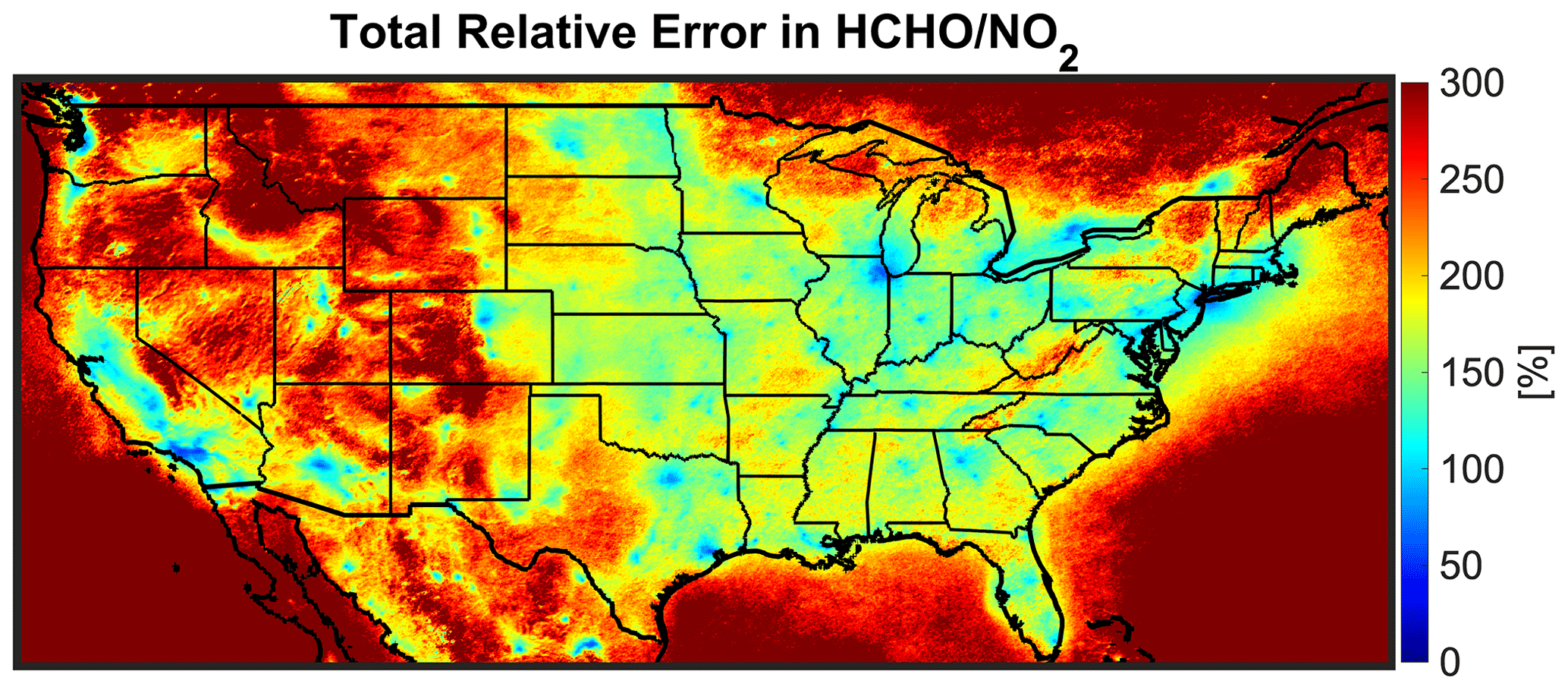
Figure 13The total relative error for observed TROPOMI ratios considering the daily TROPOMI retrieval errors (.11 × 1015 molec. cm−2 and σHCHO= 2.97 × 10¹⁵ molec. cm−2), the spatial representation pertaining to the OMI footprint over a city environment (13 % loss in the spatial variance), and the column-to-PBL translation parameterization (19 %) proposed in this study. Please note that the observed FNR is based on mean values from June to August 2021, while the uncertainties used for error calculation are on a daily basis.
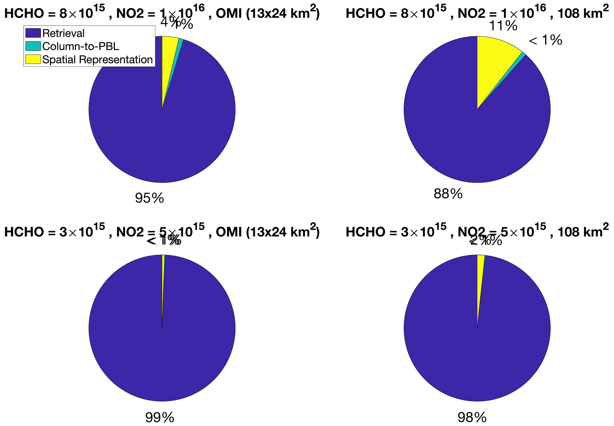
To produce some examples of the fractional errors and the combined error, we focus on two different environments with two different sets of HCHO and NO2 columns. One represents a heavily polluted area, and the other one is a moderately polluted region. We also include two footprints: OMI (13 × 24 km2) and a 108 × 108 km2 pixel. Finally, we calculate the percentage of each error component for both OMI and TROPOMI sensors. Figure 14 shows the pie charts describing the percentage of each individual error in the total error for TROPOMI. Unless the footprint of the sensor is coarse enough (e.g., 108 km2) to give rise to the spatial representation error dominance, the retrieval error stands out. New satellites are not expected to have very large footprints; as such, retrieval errors appear to be the major obstacle to using FNRs in a robust manner. Figure 15 shows the same calculation but using OMI errors; the retrieval errors massively surpass other errors. This motivates us to do one more experiment: we recalculate the HCHO error distribution in OMI using monthly-averaged data instead of daily data (Fig. S17). This experiment suggests a standard deviation of 9.4 × 10¹⁵ molec. cm−2, with which we again observe the retrieval error to be the largest contributor (> 80 %) to the combined error (Fig. S18). A recent study (Johnson et al., 2022) also suggests that retrieval errors can result in considerable disagreement between FNRs from various sensors and retrieval frameworks.
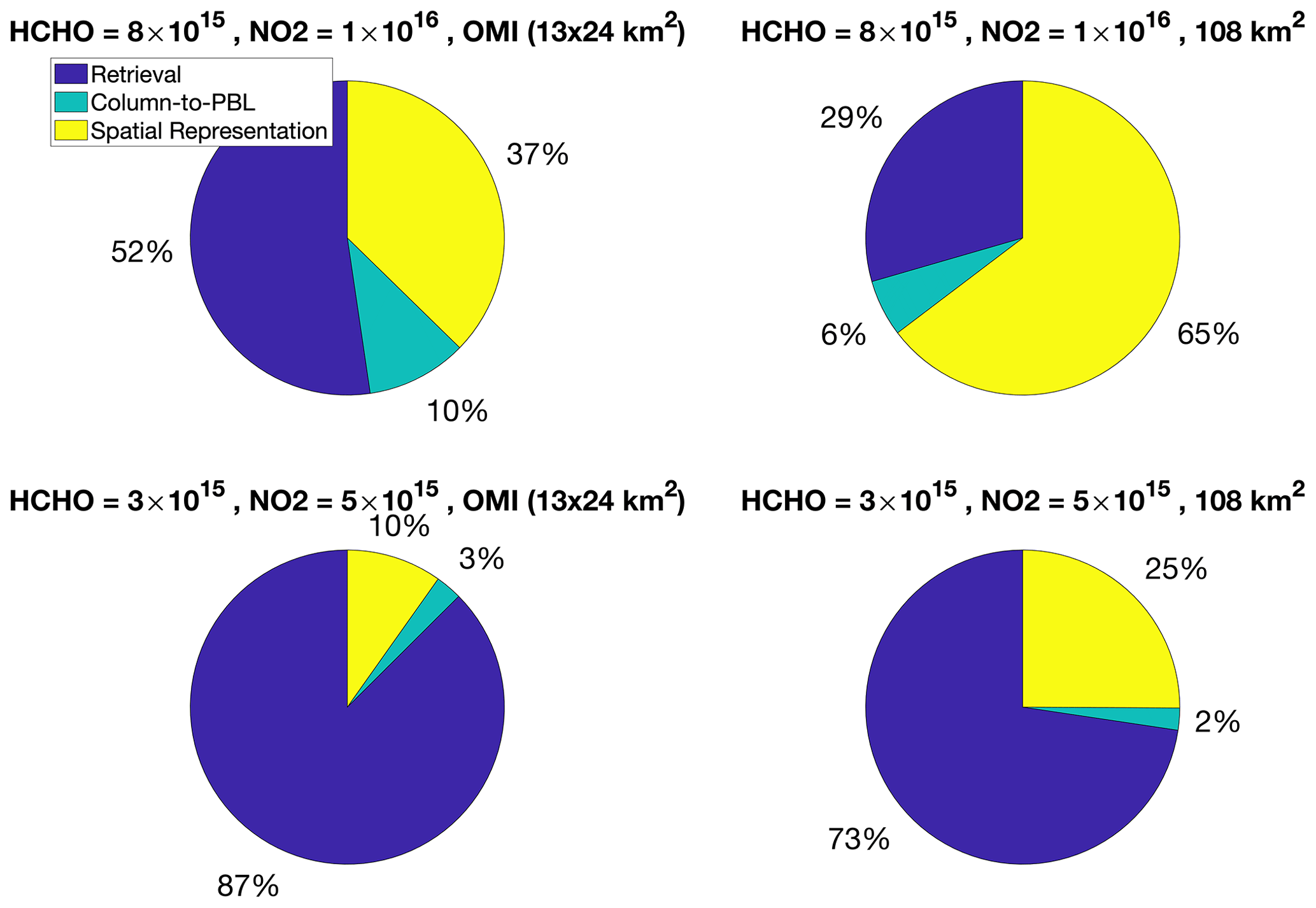
Figure 14The fractional errors of retrieval (blue), column-to-PBL translation (green), and spatial representation (yellow) of the total error budget for different concentrations and footprints based on TROPOMI sigma values. The retrieval error used for the error budget is on a daily basis.
The main goal of this study was to characterize the errors associated with the ratio of satellite-based HCHO to NO2 columns, which has been widely used for ozone sensitivity studies. From the realization of the complexity of the problem, we now know that four major errors should be carefully quantified so that we can reliably represent the underlying ozone regimes. The errors are broken down into (i) the chemistry error, (ii) the column-to-PBL translation, (iii) the spatial representation error, and (iv) the retrieval error. Each error has its own dynamics and has been tackled differently by leveraging a broad spectrum of tools and data.
The chemistry error refers to the predictive power of the ratio (hereafter FNR) in describing the HOx–ROx cycle, which can be well explained by the ratio of the chemical loss of HO2+RO2 (LROx) to the chemical loss of NOx (LNOx). Because those chemical reactions are not directly observable, we set up a chemical box model constrained with a large suite of in situ aircraft measurements collected during the DISCOVER-AQ and KORUS-AQ campaigns (∼ 500 h of flight). Our box model showed a reasonable performance in recreating some unconstrained key compounds such as OH (R2=0.64, bias = 17 %), HO2 (R2=0.66, bias < 1 %), and HCHO (R2=0.73). Subsequently, we compared the simulated FNRs to . They showed a high degree of correspondence (R2=0.93), but only on the logarithmic scale; this indicated that FNRs do not fully describe the HOx–ROx cycle (i.e., the sensitivity of ozone production rates to NOx and VOC) for heavily polluted environments and pristine ones. Following a robust baseline indicator (ln() = −1.0 ± 0.2) segregating NOx-sensitive from VOC-sensitive regimes, we observed a diverse range of FNRs ranging from 1 to 4. These transitioning ratios had a Gaussian distribution with a mean of 1.8 and a standard deviation of 0.4. This implied that the relative standard error associated with the ratio from the chemistry perspective at a 68 % confidence interval was 20 %. Although this threshold with its error was based on a single model realization and can be different for a different chemical mechanism, it provided a useful universal baseline derived from various chemical and meteorological conditions. At a 68 % confidence level, any uncertainty beyond 20 % in the ozone regime identification from FNRs likely originates from other sources of error, such as the retrieval error.
Results from the box model showed that ozone production rates in extremely polluted regions (VOC-sensitive) were not significantly different from those in pristine ones (NOx-sensitive) due to nonlinear chemical feedback mostly imposed by NO2 + OH. Indeed, the largest PO3 rates (median = 4.6 ppbv h−1) were predominantly seen in VOC-sensitive regimes tending towards the transitional regime. This was primarily caused by the abundance of ozone precursors (i.e., HCHO × NO2) and the diminished negative chemical feedback. We also revealed that HCHO × NO2 could be used as a sensible proxy for the ozone precursors' abundance. In theory, this metric, in conjunction with the ratio, provided reasonable estimates of PO3 rates (RMSE = 0.60 ppbv h−1).
We then analyzed the afternoon vertical distribution of HCHO, NO2, and their ratio observed from aircraft during the air quality campaigns binned from the near surface to 8 km. For altitudes below 5.75 km, HCHO concentration steadily decreased with altitude but at a lower rate than NO2. Above that altitude, NO2 concentrations stabilized and slightly increased due to lightning and stratospheric sources. The dissimilarity between the vertical shape of NO2 versus HCHO resulted in a rather nonlinear shape of FNRs. This nonlinear shape necessitated a mathematical formulation to transform an observed columnar ratio to a ratio at a desired vertical height expanding from the surface. We fit a second-order rational function to the profile and formulated the altitude adjustment factor, which followed a second-order polynomial function starting from values below 1 for lower altitudes, following values above 1 for some high altitudes, and finally converging to 1 at 8 km. This behavior means that the ozone regime tends to get pushed slightly towards the VOC-sensitive regime near the surface for a given tropospheric columnar ratio. This tendency was more pronounced in morning times when the nonlinear shape of FNRs was stronger. This data-driven adjustment factor exclusively derived from afternoon aircraft profiles during warm seasons under nonconvective conditions had a standard error of 19 %.
An important error in the satellite-based observations stemmed from unresolved spatial variability in trace gas concentrations within a satellite pixel (Souri et al., 2022; Tang et al., 2021). The amount of unresolved spatial variability (the spatial representation error) can in principle be modeled if we base our reference on a distribution map made from a high spatial resolution dataset. We modeled semivariograms (or spatial autocorrelation) computed for a reference map of FNRs observed by TROPOMI at 3 × 3 km2 over Los Angeles. Subsequently, we coarsened the map to 13 × 24, 36 × 36, 108 × 108, and 216 × 216 km2 and modeled their semivariograms. As for 13 × 24 km2, which is equivalent to the OMI nadir spatial resolution, around 12 % of spatial information (variance) was lost due to its footprint. The larger the footprint, the bigger the spatial representation error. For instance, a grid box with a size of 216 × 216 km2 lost 65 % of the spatial information in the ratio at a 50 km length scale. Our method is compelling to understand and easy to apply for other products and different atmospheric environments. Based on this approach, we developed an open-source package called the SpaTial Representation Error EstimaTor (STREET) (Souri, 2022).
We presented estimates of retrieval errors associated with daily TROPOMI and OMI tropospheric NO2 columns by comparing them against a large suite of MAX-DOAS (Verhoelst et al., 2021) and vertically integrated measurements from aircraft spirals (Choi et al., 2020). Both products were smaller than the benchmark. Furthermore, they show a relatively consistent dispersion at a 68 % confidence level (∼ 2 × 10¹⁵ molec. cm−2) suggested by fitting a normal function (R2 > 0.9) to their error distributions. As for daily TROPOMI and OMI HCHO products, we used global FTIR observations (Vigouroux et al., 2020) and data-constrained GEOS-Chem outputs from multiple campaigns (Zhu et al., 2020), respectively. TROPOMI HCHO indeed outperforms OMI HCHO with respect to bias and dispersion on a daily basis. The standard deviation of OMI HCHO was found to be roughly 5 times as large compared to TROPOMI. While this error can be partly reduced by oversampling over a span of a month or a season, it is critical to recognize that ozone events are episodic; thus, daily observations should be the standard mean for understanding the chemical pathways for the formation of tropospheric ozone. After combining the daily biases from both HCHO and NO2 TROPOMI comparisons, we concluded that either daily HCHO or tropospheric NO2 columns should be above 1.2–1.5 × 10¹⁶ molec. cm−2 to achieve 20 %–30 % standard error in the ratio. Due to the large error in daily OMI HCHO, it was nearly impossible to achieve 20 %–30 % standard error given the observable range of HCHO and NO2 columns over our planet. To reach 50 % error using daily OMI data, HCHO columns should be above 3.2 × 10¹⁶ molec. cm−2 or tropospheric NO2 columns should be above 8 × 10¹⁵ molec. cm−2.
To build intuition in the significance of the errors above, we finally calculated the combined error in the ratio by linearly combining the root sum of the squares of the TROPOMI retrieval errors, the spatial representation error pertaining to the OMI nadir footprint over a city-like environment, and the altitude adjustment error for a wide range of observed HCHO and NO2 columns over the US. These observations were based on TROPOMI in the summertime of 2021. The total errors were relatively mild (< 50 %) in cities due to a stronger signal, whereas they easily exceeded 100 % in regions with low vegetation and anthropogenic sources (i.e., the Rocky Mountains). The retrieval error was the dominant source of the combined error (40 %–90 %).
All of these aspects highlight the necessity of improving the trace gas satellite retrieval algorithms in conjunction with sensor calibration, although with the realization that a better retrieval is somewhat limited by the advancements made in other disciplines, such as atmospheric modeling and molecular spectroscopy.
The FTIR and MAXDOAS data used in this publication were partly obtained from the Network for the Detection of Atmospheric Composition Change (NDACC) and are available through the NDACC (2022) website at http://www.ndacc.org. The spatial representation error is estimated based on a publicly available package, the SpaTial Representation Error EstimaTor (STREET) (https://github.com/ahsouri/STREET, last access: 10 January, https://doi.org/10.5281/zenodo.7497106, Souri, 2022). DISCOVER-AQ and KORUS-AQ aircraft data can be downloaded from https://www-air.larc.nasa.gov/missions/discover-aq/discover-aq.html (DISCOVER-AQ, 2022) and https://www-air.larc.nasa.gov/missions/korus-aq/ (KORUS-AQ, 2022). TROPOMI NO2 and HCHO data can be downloaded from https://doi.org/10.5270/S5P-s4ljg54 (Koninklijk Nederlands Meteorologisch Instituut (KNMI), 2018) and https://doi.org/10.5270/S5P-tjlxfd2 (German Aerospace Center (DLR), 2019). The box model results can be obtained by contacting the corresponding author at a.souri@nasa.gov.
The supplement related to this article is available online at: https://doi.org/10.5194/acp-23-1963-2023-supplement.
AHS designed the research, analyzed the data, conducted the simulations, made all the figures, and wrote the paper. MSJ, SP, XL, and KC helped with conceptualization, fund raising, and analysis. GMW helped with configuring the box model. AF, AW, WB, DRB, AJW, RCC, KM, and CC measured various compounds during the air quality campaigns. JHC orchestrated all these campaigns and contributed to the model interpretation. TV, SC, and GP provided paired MAX-DOAS and TROPOMI tropospheric NO2 observations. CV and BL provided paired FTIR and TROPOMI HCHO observations. SC and LL provided paired integrated aircraft spirals and OMI tropospheric NO2 observations. LZ and SS provided the paired observations between the corrected GEOS-Chem HCHO and OMI HCHO columns. All the authors contributed to the discussion and edited the paper.
The contact author has declared that none of the authors has any competing interests.
Publisher's note: Copernicus Publications remains neutral with regard to jurisdictional claims in published maps and institutional affiliations.
The PTR-MS instrument team (Philipp Eichler, Lisa Kaser, Tomas Mikoviny, and Markus Müller) are thanked for their support with field work and data processing. We thank the FTIR HCHO measurement team of Thomas Blumenstock, Martine De Mazière, Michel Grutter, James W. Hannigan, Nicholas Jones, Rigel Kivi, Erik Lutsch, Emmanuel Mahieu, Maria Makarova, Isamu Morino, Isao Murata, Tomoo Nagahama, Justus Notholt, Ivan Ortega, Mathias Palm, Amelie Röhling, Matthias Schneider, Dan Smale, Wolfgang Stremme, Kim String, Youwen Sun, Ralf Sussmann, Yao Té, and Pucai Wang. We thank the Meteorological Service Suriname and Cornelis Becker for their support. The MAX-DOAS data used in this publication were obtained from Alkis Bais, John Burrows, Ka Lok Chan, Michel Grutter, Cheng Liu, Hitoshi Irie, Vinod Kumar, Yugo Kanaya, Ankie Piters, Claudia Rivera-Cárdenas, Andreas Richter, Michel Van Roozendael, Robert Ryan, Vinayak Sinha, and Thomas Wagner. Fast delivery of MAX-DOAS data tailored to the S5P validation was organized through S5PVT AO project NID-FORVAL. We thank the IISER Mohali atmospheric chemistry facility for supporting the MAX-DOAS measurements at Mohali, India. We thank Glenn Diskin for providing CO, CO2, and CH4 measurements. We thank Paul Wennberg for H2O2 and HNO3 measurements.
This study was funded by NASA’s Aura Science Team (grant no. 80NSSC21K1333). PTR-MS measurements were supported by the Austrian Federal Ministry for Transport, Innovation, and Technology (bmvit, FFG-ALR-ASAP). The measurements at Paramaribo have been supported by the BMBF (German Ministry of Education and Research) in project ROMIC-II’s subproject TroStra (01LG1904A). The NDACC FTIR stations Bremen, Garmisch, Izaña, Ny-Ålesund, Paramaribo, and Karlsruhe have been supported by the German Bundesministerium für Wirtschaft und Energie (BMWi) via DLR5 under grants 50EE1711A, B, and D. The measurements and data analysis at Bremen are supported by the Senate of Bremen. The NCAR FTS observation programs at Thule, GR, Boulder, CO, and Mauna Loa, HI, are supported under contract by the National Aeronautics and Space Administration (NASA). The National Center for Atmospheric Research is sponsored by the National Science Foundation. The Thule effort is also supported by the NSF Office of Polar Programs (OPP). Operations at the Rikubetsu and Tsukuba FTIR sites are supported in part by the GOSAT series project. The Paris TCCON site has received funding from Sorbonne Université, the French research center CNRS, and the French space agency CNES. The Jungfraujoch FTIR data are primarily available thanks to the support provided by the F.R.S. FNRS (Brussels), the GAW-CH program of MeteoSwiss (Zürich), and the HFSJG.ch Foundation (Bern). IUP-Bremen ground-based measurements are funded by DLR-Bonn and received through project 50EE1709A. KNMI ground-based measurements in De Bilt and Cabauw are partly supported by the Ruisdael Observatory project, Dutch Research Council (NWO) contract 184.034.015, by the Netherlands Space Office (NSO) for Sentinel-5p/TROPOMI validation, and by ESA via the EU CAMS project. Lei Zhu and Shuai Sun were supported by grants from the Guangdong Basic and Applied Basic Research Foundation (2021A1515110713) and Shenzhen Science and Technology Program (JCYJ20210324104604012). The TROPOMI validation work was supported by BELSPO/ESA through ProDEx project TROVA-E2 (grant no. PEA 4000116692). Tijl Verhoelst was supported by BELSPO through BRAIN-BE 2.0 project LEGO-BEL-AQ (contract B2/191/P1/LEGO-BEL-AQ).
This paper was edited by Andreas Richter and reviewed by two anonymous referees.
Ahmadov, R., McKeen, S., Trainer, M., Banta, R., Brewer, A., Brown, S., Edwards, P. M., de Gouw, J. A., Frost, G. J., Gilman, J., Helmig, D., Johnson, B., Karion, A., Koss, A., Langford, A., Lerner, B., Olson, J., Oltmans, S., Peischl, J., Pétron, G., Pichugina, Y., Roberts, J. M., Ryerson, T., Schnell, R., Senff, C., Sweeney, C., Thompson, C., Veres, P. R., Warneke, C., Wild, R., Williams, E. J., Yuan, B., and Zamora, R.: Understanding high wintertime ozone pollution events in an oil- and natural gas-producing region of the western US, Atmos. Chem. Phys., 15, 411–429, https://doi.org/10.5194/acp-15-411-2015, 2015.
Boeke, N. L., Marshall, J. D., Alvarez, S., Chance, K. V., Fried, A., Kurosu, T. P., Rappenglück, B., Richter, D., Walega, J., Weibring, P., and Millet, D. B.: Formaldehyde columns from the Ozone Monitoring Instrument: Urban versus background levels and evaluation using aircraft data and a global model, J. Geophys. Res., 116, D05303, https://doi.org/10.1029/2010JD014870, 2011.
Boersma, K. F., Eskes, H. J., and Brinksma, E. J.: Error analysis for tropospheric NO2 retrieval from space, J. Geophys. Res., 109, D04311, https://doi.org/10.1029/2003JD003962, 2004.
Boersma, K. F., Eskes, H. J., Veefkind, J. P., Brinksma, E. J., van der A, R. J., Sneep, M., van den Oord, G. H. J., Levelt, P. F., Stammes, P., Gleason, J. F., and Bucsela, E. J.: Near-real time retrieval of tropospheric NO2 from OMI, Atmos. Chem. Phys., 7, 2103–2118, https://doi.org/10.5194/acp-7-2103-2007, 2007.
Boersma, K. F., Eskes, H. J., Richter, A., De Smedt, I., Lorente, A., Beirle, S., van Geffen, J. H. G. M., Zara, M., Peters, E., Van Roozendael, M., Wagner, T., Maasakkers, J. D., van der A, R. J., Nightingale, J., De Rudder, A., Irie, H., Pinardi, G., Lambert, J.-C., and Compernolle, S. C.: Improving algorithms and uncertainty estimates for satellite NO2 retrievals: results from the quality assurance for the essential climate variables (QA4ECV) project, Atmos. Meas. Tech., 11, 6651–6678, https://doi.org/10.5194/amt-11-6651-2018, 2018.
Box, G. E. P.: Science and Statistics, J. Am. Stat. Assoc., 71, 791–799, https://doi.org/10.1080/01621459.1976.10480949, 1976.
Brune, W. H., Miller, D. O., Thames, A. B., Brosius, A. L., Barletta, B., Blake, D. R., Blake, N. J., Chen, G., Choi, Y., Crawford, J. H., Digangi, J. P., Diskin, G., Fried, A., Hall, S. R., Hanisco, T. F., Huey, G. L., Hughes, S. C., Kim, M., Meinardi, S., Montzka, D. D., Pusede, S. E., Schroeder, J. R., Teng, A., Tanner, D. J., Ullmann, K., Walega, J., Weinheimer, A., Wisthaler, A., and Wennberg, P. O.: Observations of atmospheric oxidation and ozone production in South Korea, Atmos. Environ., 269, 118854, https://doi.org/10.1016/j.atmosenv.2021.118854, 2022.
Chan, K. L., Wang, Z., Ding, A., Heue, K.-P., Shen, Y., Wang, J., Zhang, F., Shi, Y., Hao, N., and Wenig, M.: MAX-DOAS measurements of tropospheric NO2 and HCHO in Nanjing and a comparison to ozone monitoring instrument observations, Atmos. Chem. Phys., 19, 10051–10071, https://doi.org/10.5194/acp-19-10051-2019, 2019.
Chance, K., Palmer, P. I., Spurr, R. J. D., Martin, R. V., Kurosu, T. P., and Jacob, D. J.: Satellite observations of formaldehyde over North America from GOME, Geophys. Res. Lett., 27, 3461–3464, https://doi.org/10.1029/2000GL011857, 2000.
Chance, K., Liu, X., Miller, C. C., Abad, G. G., Huang, G., Nowlan, C., Souri, A., Suleiman, R., Sun, K., Wang, H., Zhu, L., Zoogman, P., Al-Saadi, J., Antuña-Marrero, J.-C., Carr, J., Chatfield, R., Chin, M., Cohen, R., Edwards, D., Fishman, J., Flittner, D., Geddes, J., Grutter, M., Herman, J. R., Jacob, D. J., Janz, S., Joiner, J., Kim, J., Krotkov, N. A., Lefer, B., Martin, R. V., Mayol-Bracero, O. L., Naeger, A., Newchurch, M., Pfister, G. G., Pickering, K., Pierce, R. B., Cárdenas, C. R., Saiz-Lopez, A., Simpson, W., Spinei, E., Spurr, R. J. D., Szykman, J. J., Torres, O., and Wang, J.: TEMPO Green Paper: Chemistry, physics, and meteorology experiments with the Tropospheric Emissions: monitoring of pollution instrument, in: Sensors, Systems, and Next-Generation Satellites XXIII, Sensors, Systems, and Next-Generation Satellites XXIII, 56–67, https://doi.org/10.1117/12.2534883, 2019.
Chance, K. V., Burrows, J. P., and Schneider, W.: Retrieval and molecule sensitivity studies for the global ozone monitoring experiment and the scanning imaging absorption spectrometer for atmospheric chartography, in: Remote Sensing of Atmospheric Chemistry, Remote Sens. Atmos. Chem., 1491, 151–165, https://doi.org/10.1117/12.46657, 1991.
Chance, K. V., Burrows, J. P., Perner, D., and Schneider, W.: Satellite measurements of atmospheric ozone profiles, including tropospheric ozone, from ultraviolet/visible measurements in the nadir geometry: a potential method to retrieve tropospheric ozone, J. Quant. Spectrosc. Ra., 57, 467–476, https://doi.org/10.1016/S0022-4073(96)00157-4, 1997.
Choi, S., Lamsal, L. N., Follette-Cook, M., Joiner, J., Krotkov, N. A., Swartz, W. H., Pickering, K. E., Loughner, C. P., Appel, W., Pfister, G., Saide, P. E., Cohen, R. C., Weinheimer, A. J., and Herman, J. R.: Assessment of NO2 observations during DISCOVER-AQ and KORUS-AQ field campaigns, Atmos. Meas. Tech., 13, 2523–2546, https://doi.org/10.5194/amt-13-2523-2020, 2020.
Choi, Y. and Souri, A. H.: Chemical condition and surface ozone in large cities of Texas during the last decade: Observational evidence from OMI, CAMS, and model analysis, Remote Sens. Environ., 168, 90–101, https://doi.org/10.1016/j.rse.2015.06.026, 2015a.
Choi, Y. and Souri, A. H.: Seasonal behavior and long-term trends of tropospheric ozone, its precursors and chemical conditions over Iran: A view from space, Atmos. Environ., 106, 232–240, https://doi.org/10.1016/j.atmosenv.2015.02.012, 2015b.
Choi, Y., Kim, H., Tong, D., and Lee, P.: Summertime weekly cycles of observed and modeled NOx and O3 concentrations as a function of satellite-derived ozone production sensitivity and land use types over the Continental United States, Atmos. Chem. Phys., 12, 6291–6307, https://doi.org/10.5194/acp-12-6291-2012, 2012.
Crawford, J. H., Ahn, J.-Y., Al-Saadi, J., Chang, L., Emmons, L. K., Kim, J., Lee, G., Park, J.-H., Park, R. J., Woo, J. H., Song, C.-K., Hong, J.-H., Hong, Y.-D., Lefer, B. L., Lee, M., Lee, T., Kim, S., Min, K.-E., Yum, S. S., Shin, H. J., Kim, Y.-W., Choi, J.-S., Park, J.-S., Szykman, J. J., Long, R. W., Jordan, C. E., Simpson, I. J., Fried, A., Dibb, J. E., Cho, S., and Kim, Y. P.: The Korea–United States Air Quality (KORUS-AQ) field study, Elem. Sci. Anth., 9, 00163, https://doi.org/10.1525/elementa.2020.00163, 2021.
de Gouw, J. A., Gilman, J. B., Kim, S.-W., Alvarez, S. L., Dusanter, S., Graus, M., Griffith, S. M., Isaacman-VanWertz, G., Kuster, W. C., Lefer, B. L., Lerner, B. M., McDonald, B. C., Rappenglück, B., Roberts, J. M., Stevens, P. S., Stutz, J., Thalman, R., Veres, P. R., Volkamer, R., Warneke, C., Washenfelder, R. A., and Young, C. J.: Chemistry of Volatile Organic Compounds in the Los Angeles Basin: Formation of Oxygenated Compounds and Determination of Emission Ratios, J. Geophys. Res.-Atmos., 123, 2298–2319, https://doi.org/10.1002/2017JD027976, 2018.
De Smedt, I., Müller, J.-F., Stavrakou, T., van der A, R., Eskes, H., and Van Roozendael, M.: Twelve years of global observations of formaldehyde in the troposphere using GOME and SCIAMACHY sensors, Atmos. Chem. Phys., 8, 4947–4963, https://doi.org/10.5194/acp-8-4947-2008, 2008.
De Smedt, I., Stavrakou, T., Müller, J.-F., van der A, R. J., and Van Roozendael, M.: Trend detection in satellite observations of formaldehyde tropospheric columns, Geophys. Res. Lett., 37, L18808, https://doi.org/10.1029/2010GL044245, 2010.
De Smedt, I., Stavrakou, T., Hendrick, F., Danckaert, T., Vlemmix, T., Pinardi, G., Theys, N., Lerot, C., Gielen, C., Vigouroux, C., Hermans, C., Fayt, C., Veefkind, P., Müller, J.-F., and Van Roozendael, M.: Diurnal, seasonal and long-term variations of global formaldehyde columns inferred from combined OMI and GOME-2 observations, Atmos. Chem. Phys., 15, 12519–12545, https://doi.org/10.5194/acp-15-12519-2015, 2015.
De Smedt, I., Theys, N., Yu, H., Danckaert, T., Lerot, C., Compernolle, S., Van Roozendael, M., Richter, A., Hilboll, A., Peters, E., Pedergnana, M., Loyola, D., Beirle, S., Wagner, T., Eskes, H., van Geffen, J., Boersma, K. F., and Veefkind, P.: Algorithm theoretical baseline for formaldehyde retrievals from S5P TROPOMI and from the QA4ECV project, Atmos. Meas. Tech., 11, 2395–2426, https://doi.org/10.5194/amt-11-2395-2018, 2018.
De Smedt, I., Pinardi, G., Vigouroux, C., Compernolle, S., Bais, A., Benavent, N., Boersma, F., Chan, K.-L., Donner, S., Eichmann, K.-U., Hedelt, P., Hendrick, F., Irie, H., Kumar, V., Lambert, J.-C., Langerock, B., Lerot, C., Liu, C., Loyola, D., Piters, A., Richter, A., Rivera Cárdenas, C., Romahn, F., Ryan, R. G., Sinha, V., Theys, N., Vlietinck, J., Wagner, T., Wang, T., Yu, H., and Van Roozendael, M.: Comparative assessment of TROPOMI and OMI formaldehyde observations and validation against MAX-DOAS network column measurements, Atmos. Chem. Phys., 21, 12561–12593, https://doi.org/10.5194/acp-21-12561-2021, 2021.
Diao, L., Choi, Y., Czader, B., Li, X., Pan, S., Roy, A., Souri, A. H., Estes, M., and Jeon, W.: Discrepancies between modeled and observed nocturnal isoprene in an urban environment and the possible causes: A case study in Houston, Atmos. Res., 181, 257–264, https://doi.org/10.1016/j.atmosres.2016.07.009, 2016.
DISCOVER-AQ: Deriving Information on Surface Conditions from COlumn and VERtically Resolved Observations Relevant to Air Quality (DISCOVER-AQ), NASA Langley Research Center, VA, USA [data set], https://www-air.larc.nasa.gov/missions/discover-aq/discover-aq.html, last of access: 5 June 2022.
Duncan, B. N., Yoshida, Y., Olson, J. R., Sillman, S., Martin, R. V., Lamsal, L., Hu, Y., Pickering, K. E., Retscher, C., Allen, D. J., and Crawford, J. H.: Application of OMI observations to a space-based indicator of NOx and VOC controls on surface ozone formation, Atmos. Environ., 44, 2213–2223, https://doi.org/10.1016/j.atmosenv.2010.03.010, 2010.
Fried, A., Walega, J., Weibring, P., Richter, D., Simpson, I. J., Blake, D. R., Blake, N. J., Meinardi, S., Barletta, B., Hughes, S. C., Crawford, J. H., Diskin, G., Barrick, J., Hair, J., Fenn, M., Wisthaler, A., Mikoviny, T., Woo, J.-H., Park, M., Kim, J., Min, K.-E., Jeong, S., Wennberg, P. O., Kim, M. J., Crounse, J. D., Teng, A. P., Bennett, R., Yang-Martin, M., Shook, M. A., Huey, G., Tanner, D., Knote, C., Kim, J., Park, R., and Brune, W.: Airborne formaldehyde and volatile organic compound measurements over the Daesan petrochemical complex on Korea's northwest coast during the Korea-United States Air Quality study: Estimation of emission fluxes and effects on air quality, Elem. Sci. Anth., 8, 121, https://doi.org/10.1525/elementa.2020.121, 2020.
German Aerospace Center (DLR): Copernicus Sentinel data processed by ESA, Sentinel-5P TROPOMI Tropospheric Formaldehyde HCHO 1-Orbit L2 7km x 3.5km, Greenbelt, MD, USA, Goddard Earth Sciences Data and Information Services Center (GES DISC) [data set], https://doi.org/10.5270/S5P-tjlxfd2, 2019.
González Abad, G., Liu, X., Chance, K., Wang, H., Kurosu, T. P., and Suleiman, R.: Updated Smithsonian Astrophysical Observatory Ozone Monitoring Instrument (SAO OMI) formaldehyde retrieval, Atmos. Meas. Tech., 8, 19–32, https://doi.org/10.5194/amt-8-19-2015, 2015.
González Abad, G., Souri, A. H., Bak, J., Chance, K., Flynn, L. E., Krotkov, N. A., Lamsal, L., Li, C., Liu, X., Miller, C. C., Nowlan, C. R., Suleiman, R., and Wang, H.: Five decades observing Earth's atmospheric trace gases using ultraviolet and visible backscatter solar radiation from space, J. Quant. Spectrosc. Ra., 238, 106478, https://doi.org/10.1016/j.jqsrt.2019.04.030, 2019.
Janjić, T., Bormann, N., Bocquet, M., Carton, J. A., Cohn, S. E., Dance, S. L., Losa, S. N., Nichols, N. K., Potthast, R., Waller, J. A., and Weston, P.: On the representation error in data assimilation, Q. J. Roy. Meteor. Soc., 144, 1257–1278, https://doi.org/10.1002/qj.3130, 2018.
Jeon, W., Choi, Y., Souri, A. H., Roy, A., Diao, L., Pan, S., Lee, H. W., and Lee, S.-H.: Identification of chemical fingerprints in long-range transport of burning induced upper tropospheric ozone from Colorado to the North Atlantic Ocean, Sci. Total Environ., 613–614, 820–828, https://doi.org/10.1016/j.scitotenv.2017.09.177, 2018.
Jin, X. and Holloway, T.: Spatial and temporal variability of ozone sensitivity over China observed from the Ozone Monitoring Instrument, J. Geophys. Res.-Atmos., 120, 7229–7246, https://doi.org/10.1002/2015JD023250, 2015.
Jin, X., Fiore, A. M., Murray, L. T., Valin, L. C., Lamsal, L. N., Duncan, B., Folkert Boersma, K., De Smedt, I., Abad, G. G., Chance, K., and Tonnesen, G. S.: Evaluating a Space-Based Indicator of Surface Ozone-NOx-VOC Sensitivity Over Midlatitude Source Regions and Application to Decadal Trends, J. Geophys. Res.-Atmos., 122, 10439–10461, https://doi.org/10.1002/2017JD026720, 2017.
Johnson, M. S., Philip, S., Kumar, R., Naeger, A., Souri, A. H., Geddes, J., Judd, L., Janz, S., and Sullivan, J.: Satellite remote-sensing capability to assess tropospheric column ratios of formaldehyde and nitrogen dioxide: case study during the LISTOS 2018 field campaign, Atmos. Meas. Tech. Discuss. [preprint], https://doi.org/10.5194/amt-2022-237, in review, 2022.
Kleinman, L. I., Daum, P. H., Lee, Y.-N., Nunnermacker, L. J., Springston, S. R., Weinstein-Lloyd, J., and Rudolph, J.: Sensitivity of ozone production rate to ozone precursors, Geophys. Res. Lett., 28, 2903–2906, https://doi.org/10.1029/2000GL012597, 2001.
Koninklijk Nederlands Meteorologisch Instituut (KNMI): Copernicus Sentinel data processed by ESA, Sentinel-5P TROPOMI Tropospheric NO2 1-Orbit L2 7km x 3.5km, Greenbelt, MD, USA, Goddard Earth Sciences Data and Information Services Center (GES DISC) [data set], https://doi.org/10.5270/S5P-s4ljg54, 2018.
KORUS-AQ: The Korean and United States (KORUS), NASA Langley Research Center, VA, USA [data set], https://www-air.larc.nasa.gov/missions/korus-aq/, last access: 5 June 2022.
Laughner, J. L., Zhu, Q., and Cohen, R. C.: Evaluation of version 3.0B of the BEHR OMI NO2 product, Atmos. Meas. Tech., 12, 129–146, https://doi.org/10.5194/amt-12-129-2019, 2019.
Lee, H.-J., Chang, L.-S., Jaffe, D. A., Bak, J., Liu, X., Abad, G. G., Jo, H.-Y., Jo, Y.-J., Lee, J.-B., Yang, G.-H., Kim, J.-M., and Kim, C.-H.: Satellite-Based Diagnosis and Numerical Verification of Ozone Formation Regimes over Nine Megacities in East Asia, Remote Sens., 14, 1285, https://doi.org/10.3390/rs14051285, 2022.
Lee, Y., Huey, L. G., Wang, Y., Qu, H., Zhang, R., Ji, Y., Tanner, D. J., Wang, X., Tang, J., Song, W., Hu, W., and Zhang, Y.: Photochemistry of Volatile Organic Compounds in the Yellow River Delta, China: Formation of O3 and Peroxyacyl Nitrates, J. Geophys. Res. Atmos., 126, e2021JD035296, https://doi.org/10.1029/2021JD035296, 2021.
Lorente, A., Folkert Boersma, K., Yu, H., Dörner, S., Hilboll, A., Richter, A., Liu, M., Lamsal, L. N., Barkley, M., De Smedt, I., Van Roozendael, M., Wang, Y., Wagner, T., Beirle, S., Lin, J.-T., Krotkov, N., Stammes, P., Wang, P., Eskes, H. J., and Krol, M.: Structural uncertainty in air mass factor calculation for NO2 and HCHO satellite retrievals, Atmos. Meas. Tech., 10, 759–782, https://doi.org/10.5194/amt-10-759-2017, 2017.
Martin, R. V., Chance, K., Jacob, D. J., Kurosu, T. P., Spurr, R. J. D., Bucsela, E., Gleason, J. F., Palmer, P. I., Bey, I., Fiore, A. M., Li, Q., Yantosca, R. M., and Koelemeijer, R. B. A.: An improved retrieval of tropospheric nitrogen dioxide from GOME, J. Geophys. Res., 107, 4437, https://doi.org/10.1029/2001JD001027, 2002.
Martin, R. V., Fiore, A. M., and Van Donkelaar, A.: Space-based diagnosis of surface ozone sensitivity to anthropogenic emissions, Geophys. Res. Lett., 31, L06120, https://doi.org/10.1029/2004GL019416, 2004.
Matheron, G.: Principles of geostatistics, Econ. Geol., 58, 1246–1266, https://doi.org/10.2113/gsecongeo.58.8.1246, 1963.
Miller, D. O. and Brune, W. H.: Investigating the Understanding of Oxidation Chemistry Using 20 Years of Airborne OH and HO2 Observations, J. Geophys. Res.-Atmos., 127, e2021JD035368, https://doi.org/10.1029/2021JD035368, 2022.
Newland, M. J., Bryant, D. J., Dunmore, R. E., Bannan, T. J., Acton, W. J. F., Langford, B., Hopkins, J. R., Squires, F. A., Dixon, W., Drysdale, W. S., Ivatt, P. D., Evans, M. J., Edwards, P. M., Whalley, L. K., Heard, D. E., Slater, E. J., Woodward-Massey, R., Ye, C., Mehra, A., Worrall, S. D., Bacak, A., Coe, H., Percival, C. J., Hewitt, C. N., Lee, J. D., Cui, T., Surratt, J. D., Wang, X., Lewis, A. C., Rickard, A. R., and Hamilton, J. F.: Low-NO atmospheric oxidation pathways in a polluted megacity, Atmos. Chem. Phys., 21, 1613–1625, https://doi.org/10.5194/acp-21-1613-2021, 2021.
NDACC: Network for the Detection of Atmospheric Composition Change, NDACC [data set], http://www.ndacc.org, last access: 5 June 2022.
Nowlan, C. R., Liu, X., Janz, S. J., Kowalewski, M. G., Chance, K., Follette-Cook, M. B., Fried, A., González Abad, G., Herman, J. R., Judd, L. M., Kwon, H.-A., Loughner, C. P., Pickering, K. E., Richter, D., Spinei, E., Walega, J., Weibring, P., and Weinheimer, A. J.: Nitrogen dioxide and formaldehyde measurements from the GEOstationary Coastal and Air Pollution Events (GEO-CAPE) Airborne Simulator over Houston, Texas, Atmos. Meas. Tech., 11, 5941–5964, https://doi.org/10.5194/amt-11-5941-2018, 2018.
Nunnermacker, L. J., Weinstein-Lloyd, J., Kleinman, L., Daum, P. H., Lee, Y. N., Springston, S. R., Klotz, P., Newman, L., Neuroth, G., and Hyde, P.: Ground-based and aircraft measurements of trace gases in Phoenix, Arizona (1998), Atmos. Environ., 38, 4941–4956, https://doi.org/10.1016/j.atmosenv.2004.04.033, 2004.
Pan, S., Choi, Y., Roy, A., Li, X., Jeon, W., and Souri, A. H.: Modeling the uncertainty of several VOC and its impact on simulated VOC and ozone in Houston, Texas, Atmos. Environ., 120, 404–416, https://doi.org/10.1016/j.atmosenv.2015.09.029, 2015.
Rappenglück, B., Ackermann, L., Alvarez, S., Golovko, J., Buhr, M., Field, R. A., Soltis, J., Montague, D. C., Hauze, B., Adamson, S., Risch, D., Wilkerson, G., Bush, D., Stoeckenius, T., and Keslar, C.: Strong wintertime ozone events in the Upper Green River basin, Wyoming, Atmos. Chem. Phys., 14, 4909–4934, https://doi.org/10.5194/acp-14-4909-2014, 2014.
Ren, B., Xie, P., Xu, J., Li, A., Qin, M., Hu, R., Zhang, T., Fan, G., Tian, X., Zhu, W., Hu, Z., Huang, Y., Li, X., Meng, F., Zhang, G., Tong, J., Ren, H., Zheng, J., Zhang, Z., and Lv, Y.: Vertical characteristics of NO2 and HCHO, and the ozone formation regimes in Hefei, China, Sci. Total Environ., 823, 153425, https://doi.org/10.1016/j.scitotenv.2022.153425, 2022.
Schroeder, J. R., Crawford, J. H., Fried, A., Walega, J., Weinheimer, A., Wisthaler, A., Müller, M., Mikoviny, T., Chen, G., Shook, M., Blake, D. R., and Tonnesen, G. S.: New insights into the column CH2O/NO2 ratio as an indicator of near-surface ozone sensitivity, J. Geophys. Res.-Atmos., 122, 8885–8907, https://doi.org/10.1002/2017JD026781, 2017.
Schroeder, J. R., Crawford, J. H., Ahn, J.-Y., Chang, L., Fried, A., Walega, J., Weinheimer, A., Montzka, D. D., Hall, S. R., Ullmann, K., Wisthaler, A., Mikoviny, T., Chen, G., Blake, D. R., Blake, N. J., Hughes, S. C., Meinardi, S., Diskin, G., Digangi, J. P., Choi, Y., Pusede, S. E., Huey, G. L., Tanner, D. J., Kim, M., and Wennberg, P.: Observation-based modeling of ozone chemistry in the Seoul metropolitan area during the Korea-United States Air Quality Study (KORUS-AQ), Elem. Sci. Anth., 8, 3, https://doi.org/10.1525/elementa.400, 2020.
Schwaerzel, M., Emde, C., Brunner, D., Morales, R., Wagner, T., Berne, A., Buchmann, B., and Kuhlmann, G.: Three-dimensional radiative transfer effects on airborne and ground-based trace gas remote sensing, Atmos. Meas. Tech., 13, 4277–4293, https://doi.org/10.5194/amt-13-4277-2020, 2020.
Seinfeld, J. H. and Pandis, S. N.: Atmospheric Chemistry and Physics: From Air Pollution to Climate Change, 2nd Edn., Wiley-Interscience, Hoboken, N.J., ISBN 978-1-118-94740-1, 2006.
Sillman, S. and He, D.: Some theoretical results concerning O3-NOx-VOC chemistry and NOx-VOC indicators, J. Geophys. Res., 107, 4659, https://doi.org/10.1029/2001JD001123, 2002.
Sillman, S., Logan, J. A., and Wofsy, S. C.: The sensitivity of ozone to nitrogen oxides and hydrocarbons in regional ozone episodes, J. Geophys. Res., 95, 1837–1851, https://doi.org/10.1029/JD095iD02p01837, 1990.
Souri, A. H.: ahsouri/STREET: STREET 0.0.3 (0.0.3), Zenodo [code], https://doi.org/10.5281/zenodo.7497106, 2022.
Souri, A. H., Choi, Y., Jeon, W., Woo, J.-H., Zhang, Q., and Kurokawa, J.: Remote sensing evidence of decadal changes in major tropospheric ozone precursors over East Asia, J. Geophys. Res.-Atmos., 122, 2474–2492, https://doi.org/10.1002/2016JD025663, 2017.
Souri, A. H., Nowlan, C. R., Wolfe, G. M., Lamsal, L. N., Chan Miller, C. E., Abad, G. G., Janz, S. J., Fried, A., Blake, D. R., Weinheimer, A. J., Diskin, G. S., Liu, X., and Chance, K.: Revisiting the effectiveness of HCHO/NO2 ratios for inferring ozone sensitivity to its precursors using high resolution airborne remote sensing observations in a high ozone episode during the KORUS-AQ campaign, Atmos. Environ., 224, 117341, https://doi.org/10.1016/j.atmosenv.2020.117341, 2020.
Souri, A. H., Chance, K., Bak, J., Nowlan, C. R., González Abad, G., Jung, Y., Wong, D. C., Mao, J., and Liu, X.: Unraveling pathways of elevated ozone induced by the 2020 lockdown in Europe by an observationally constrained regional model using TROPOMI, Atmos. Chem. Phys., 21, 18227–18245, https://doi.org/10.5194/acp-21-18227-2021, 2021.
Souri, A. H., Chance, K., Sun, K., Liu, X., and Johnson, M. S.: Dealing with spatial heterogeneity in pointwise-to-gridded- data comparisons, Atmos. Meas. Tech., 15, 41–59, https://doi.org/10.5194/amt-15-41-2022, 2022.
Tang, W., Edwards, D. P., Emmons, L. K., Worden, H. M., Judd, L. M., Lamsal, L. N., Al-Saadi, J. A., Janz, S. J., Crawford, J. H., Deeter, M. N., Pfister, G., Buchholz, R. R., Gaubert, B., and Nowlan, C. R.: Assessing sub-grid variability within satellite pixels over urban regions using airborne mapping spectrometer measurements, Atmos. Meas. Tech., 14, 4639–4655, https://doi.org/10.5194/amt-14-4639-2021, 2021.
Thornton, J. A., Wooldridge, P. J., Cohen, R. C., Martinez, M., Harder, H., Brune, W. H., Williams, E. J., Roberts, J. M., Fehsenfeld, F. C., Hall, S. R., Shetter, R. E., Wert, B. P., and Fried, A.: Ozone production rates as a function of NOx abundances and HOx production rates in the Nashville urban plume, J. Geophys. Res., 107, ACH 7-1–ACH 7-17, https://doi.org/10.1029/2001JD000932, 2002.
Tonnesen, G. S. and Dennis, R. L.: Analysis of radical propagation efficiency to assess ozone sensitivity to hydrocarbons and NOx: 1. Local indicators of instantaneous odd oxygen production sensitivity, J. Geophys. Res., 105, 9213–9225, https://doi.org/10.1029/1999JD900371, 2000a.
Tonnesen, G. S. and Dennis, R. L.: Analysis of radical propagation efficiency to assess ozone sensitivity to hydrocarbons and NOx: 2. Long-lived species as indicators of ozone concentration sensitivity, J. Geophys. Res., 105, 9227–9241, https://doi.org/10.1029/1999JD900372, 2000b.
Valin, L. C., Russell, A. R., Hudman, R. C., and Cohen, R. C.: Effects of model resolution on the interpretation of satellite NO2 observations, Atmos. Chem. Phys., 11, 11647–11655, https://doi.org/10.5194/acp-11-11647-2011, 2011.
van Geffen, J., Eskes, H., Compernolle, S., Pinardi, G., Verhoelst, T., Lambert, J.-C., Sneep, M., ter Linden, M., Ludewig, A., Boersma, K. F., and Veefkind, J. P.: Sentinel-5P TROPOMI NO2 retrieval: impact of version v2.2 improvements and comparisons with OMI and ground-based data, Atmos. Meas. Tech., 15, 2037–2060, https://doi.org/10.5194/amt-15-2037-2022, 2022.
Verhoelst, T., Compernolle, S., Pinardi, G., Lambert, J.-C., Eskes, H. J., Eichmann, K.-U., Fjæraa, A. M., Granville, J., Niemeijer, S., Cede, A., Tiefengraber, M., Hendrick, F., Pazmiño, A., Bais, A., Bazureau, A., Boersma, K. F., Bognar, K., Dehn, A., Donner, S., Elokhov, A., Gebetsberger, M., Goutail, F., Grutter de la Mora, M., Gruzdev, A., Gratsea, M., Hansen, G. H., Irie, H., Jepsen, N., Kanaya, Y., Karagkiozidis, D., Kivi, R., Kreher, K., Levelt, P. F., Liu, C., Müller, M., Navarro Comas, M., Piters, A. J. M., Pommereau, J.-P., Portafaix, T., Prados-Roman, C., Puentedura, O., Querel, R., Remmers, J., Richter, A., Rimmer, J., Rivera Cárdenas, C., Saavedra de Miguel, L., Sinyakov, V. P., Stremme, W., Strong, K., Van Roozendael, M., Veefkind, J. P., Wagner, T., Wittrock, F., Yela González, M., and Zehner, C.: Ground-based validation of the Copernicus Sentinel-5P TROPOMI NO2 measurements with the NDACC ZSL-DOAS, MAX-DOAS and Pandonia global networks, Atmos. Meas. Tech., 14, 481–510, https://doi.org/10.5194/amt-14-481-2021, 2021.
Vigouroux, C., Langerock, B., Bauer Aquino, C. A., Blumenstock, T., Cheng, Z., De Mazière, M., De Smedt, I., Grutter, M., Hannigan, J. W., Jones, N., Kivi, R., Loyola, D., Lutsch, E., Mahieu, E., Makarova, M., Metzger, J.-M., Morino, I., Murata, I., Nagahama, T., Notholt, J., Ortega, I., Palm, M., Pinardi, G., Röhling, A., Smale, D., Stremme, W., Strong, K., Sussmann, R., Té, Y., van Roozendael, M., Wang, P., and Winkler, H.: TROPOMI–Sentinel-5 Precursor formaldehyde validation using an extensive network of ground-based Fourier-transform infrared stations, Atmos. Meas. Tech., 13, 3751–3767, https://doi.org/10.5194/amt-13-3751-2020, 2020.
Wells, K. C., Millet, D. B., Payne, V. H., Deventer, M. J., Bates, K. H., de Gouw, J. A., Graus, M., Warneke, C., Wisthaler, A., and Fuentes, J. D.: Satellite isoprene retrievals constrain emissions and atmospheric oxidation, Nature, 585, 225–233, https://doi.org/10.1038/s41586-020-2664-3, 2020.
Wolfe, G. M., Kaiser, J., Hanisco, T. F., Keutsch, F. N., de Gouw, J. A., Gilman, J. B., Graus, M., Hatch, C. D., Holloway, J., Horowitz, L. W., Lee, B. H., Lerner, B. M., Lopez-Hilifiker, F., Mao, J., Marvin, M. R., Peischl, J., Pollack, I. B., Roberts, J. M., Ryerson, T. B., Thornton, J. A., Veres, P. R., and Warneke, C.: Formaldehyde production from isoprene oxidation across NOx regimes, Atmos. Chem. Phys., 16, 2597–2610, https://doi.org/10.5194/acp-16-2597-2016, 2016a.
Wolfe, G. M., Marvin, M. R., Roberts, S. J., Travis, K. R., and Liao, J.: The Framework for 0-D Atmospheric Modeling (F0AM) v3.1, Geosci. Model Dev., 9, 3309–3319, https://doi.org/10.5194/gmd-9-3309-2016, 2016b.
Xu, W., Zhang, G., Wang, Y., Tong, S., Zhang, W., Ma, Z., Lin, W., Kuang, Y., Yin, L., and Xu, X.: Aerosol Promotes Peroxyacetyl Nitrate Formation During Winter in the North China Plain, Environ. Sci. Technol., 55, 3568–3581, https://doi.org/10.1021/acs.est.0c08157, 2021.
Yang, K., Carn, S. A., Ge, C., Wang, J., and Dickerson, R. R.: Advancing measurements of tropospheric NO2 from space: New algorithm and first global results from OMPS, Geophys. Res. Lett., 41, 4777–4786, https://doi.org/10.1002/2014GL060136, 2014.
Zhang, K., Duan, Y., Huo, J., Huang, L., Wang, Y., Fu, Q., Wang, Y., and Li, L.: Formation mechanism of HCHO pollution in the suburban Yangtze River Delta region, China: A box model study and policy implementations, Atmos. Environ., 267, 118755, https://doi.org/10.1016/j.atmosenv.2021.118755, 2021.
Zhu, L., Jacob, D. J., Mickley, L. J., Marais, E. A., Cohan, D. S., Yoshida, Y., Duncan, B. N., Abad, G. G., and Chance, K. V.: Anthropogenic emissions of highly reactive volatile organic compounds in eastern Texas inferred from oversampling of satellite (OMI) measurements of HCHO columns, Environ. Res. Lett., 9, 114004, https://doi.org/10.1088/1748-9326/9/11/114004, 2014.
Zhu, L., Jacob, D. J., Kim, P. S., Fisher, J. A., Yu, K., Travis, K. R., Mickley, L. J., Yantosca, R. M., Sulprizio, M. P., De Smedt, I., González Abad, G., Chance, K., Li, C., Ferrare, R., Fried, A., Hair, J. W., Hanisco, T. F., Richter, D., Jo Scarino, A., Walega, J., Weibring, P., and Wolfe, G. M.: Observing atmospheric formaldehyde (HCHO) from space: validation and intercomparison of six retrievals from four satellites (OMI, GOME2A, GOME2B, OMPS) with SEAC4RS aircraft observations over the southeast US, Atmos. Chem. Phys., 16, 13477–13490, https://doi.org/10.5194/acp-16-13477-2016, 2016.
Zhu, L., González Abad, G., Nowlan, C. R., Chan Miller, C., Chance, K., Apel, E. C., DiGangi, J. P., Fried, A., Hanisco, T. F., Hornbrook, R. S., Hu, L., Kaiser, J., Keutsch, F. N., Permar, W., St. Clair, J. M., and Wolfe, G. M.: Validation of satellite formaldehyde (HCHO) retrievals using observations from 12 aircraft campaigns, Atmos. Chem. Phys., 20, 12329–12345, https://doi.org/10.5194/acp-20-12329-2020, 2020.