the Creative Commons Attribution 4.0 License.
the Creative Commons Attribution 4.0 License.
 | 02 Feb 2023
Potential impact of shipping on air pollution in the Mediterranean region – a multimodel evaluation: comparison of photooxidants NO2 and O3
Matthias Karl
Volker Matthias
Sonia Oppo
Richard Kranenburg
Jeroen Kuenen
Jana Moldanova
Sara Jutterström
Jukka-Pekka Jalkanen
Elisa Majamäki
Shipping has a significant share in the emissions of air pollutants such as NOx and particulate matter (PM), and the global maritime transport volumes are projected to increase further in the future. The major route for short sea shipping within Europe and the main shipping route between Europe and East Asia are found in the Mediterranean Sea. Thus, it is a highly frequented shipping area, and high levels of air pollutants with significant potential impacts from shipping emissions are observed at monitoring stations in many cities along the Mediterranean coast.
The present study is part of the EU H2020 project SCIPPER (Shipping contribution to Inland Pollution Push for the Enforcement of Regulations). Five different regional chemistry transport models (CAMx – Comprehensive Air Quality Model with Extensions, CHIMERE, CMAQ, EMEP – European Monitoring and Evaluation Programme, LOTOS-EUROS) were used to simulate the transport, chemical transformation and fate of atmospheric pollutants in the Mediterranean Sea for 2015. Shipping emissions were calculated with the Ship Traffic Emission Assessment Model (STEAM) version 3.3.0, and land-based emissions were taken from the CAMS-REG v2.2.1 dataset for a domain covering the Mediterranean Sea at a resolution of 12 km × 12 km (or ). All models used their standard setup for further input. The potential impact of ships was calculated with the zero-out method. The model results were compared to each other and to measured background data at monitoring stations.
The model results differ regarding the time series and pattern but are similar concerning the overall underestimation of NO2 and overestimation of O3. The potential impact from ships on the total NO2 concentration was especially high on the main shipping routes and in coastal regions (25 % to 85 %). The potential impact from ships on the total O3 concentration was lowest in regions with the highest NO2 impact (down to −20%). CAMx and CHIMERE simulated the highest potential impacts of ships on the NO2 and O3 air concentrations. Additionally, the strongest correlation was found between CAMx and CHIMERE, which can be traced back to the use of the same meteorological input data. The other models used different meteorological input due to their standard setup. The CMAQ-, EMEP- and LOTOS-EUROS-simulated values were within one range for the NO2 and O3 air concentrations. Regarding simulated deposition, larger differences between the models were found when compared to air concentration. These uncertainties and deviations between models are caused by deposition mechanisms, which are unique within each model. A reliable output from models simulating ships' potential impacts can be expected for air concentrations of NO2 and O3.
- Article
(10723 KB) - Full-text XML
-
Supplement
(1886 KB) - BibTeX
- EndNote


Shipping activity and freight transport via ships are growing, and previous studies have shown that the relative potential impact from shipping to total air pollution will also increase (Brandt et al., 2013). Once in the atmosphere, these emissions are transported over several hundreds of kilometers, with 70 % of shipping emissions occurring less than 400 km from the coast (Eyring et al., 2010; Endresen et al., 2003). Several previous studies have pointed out the negative effect of shipping emissions on the concentration of air pollutants, playing a role as greenhouse gases, impacting human health, or contributing to acidification and eutrophication (Tysro and Berge, 1997; Corbett and Fischbeck, 1997; Corbett et al., 1999). An overview over the current knowledge of effects of shipping on air quality and the human health worldwide is given in a review by Contini et al. (2021). Nevertheless, maritime transport plays a vital role in the international trade of goods worldwide as well as in the European Union (EU). The Eurostat Press Office (2016) stated that for 2015, the value of EU trade of goods with non-EU countries transported by the sea was approximately 51 % of EU traded goods. The Mediterranean Sea serves as both the primary shipping route between Europe and East Asia and the principal route for short sea shipping within Europe. It is the region in Europe with maximal impact from shipping emissions to gaseous pollutants, in addition to the North Sea (Viana et al., 2014).
Additionally, as one of the fastest growing sources of greenhouse gas emissions, shipping emissions directly result in health problems and have adverse effects on ecosystems (Brandt et al., 2013). The wide range of gaseous pollutants, such as nitrogen oxides (), coming from shipping emissions have negative impacts by forming smog and acid rain and contribute to eutrophication (Jägerbrand et al., 2019; Brandt et al., 2013; Karl et al., 2019a; Matthias et al., 2010).
Moreover, NOx, as a primary pollutant, plays an important role in the formation of O3 and in the deposition of reactive nitrogen compounds (Eyring et al., 2010). The oxidation of VOCs (volatile organic compounds) produces ozone in the troposphere when NOx and sunlight are present. O3 can inflame and damage the respiratory system, make the lungs more susceptible to infection, and intensify lung diseases (EPA, 2021). Although it is not directly emitted, O3 is an important compound in photochemistry. Especially in the Mediterranean Sea during summer, when radiation is high, the contribution of shipping emissions to mean surface O3 concentrations can be significant (Aksoyoglu et al., 2016).
Atmospheric nitrogen deposition mainly comes from agricultural activities and combustion processes such as those in shipping (Aksoyoglu et al., 2016). This increase in bioavailable nitrogen deposition causes eutrophication (Jägerbrand et al., 2019). The deposition of O3 affects a plant's stomata, damages plants, changes water and carbon cycling, and reduces crop yields (Clifton et al., 2020).
Chemistry transport models (CTMs) can be applied to simulate the transport of air pollutants as well as chemical transformation and deposition. These models can be used at different scales, depending on the domain they cover and the question to be answered.
Although shipping emissions have a significant impact on air pollution by NO2 in the Mediterranean Sea (Marmer and Langmann, 2005), few regional-scale chemistry transport modeling studies have focused on this domain. A literature review study focusing on the assessment of the impacts of shipping emissions on air quality in European coastal areas by Viana et al. (2014) showed that studies regarding shipping emissions in the Mediterranean Sea emphasize PM levels and their chemical composition instead of gaseous pollutants. Marmer and Langmann (2005) investigated the Mediterranean Sea but on a larger scale or without the comparison of different CTMs. Other studies focus on smaller domains over the Iberian Peninsula (Baldasano et al., 2011; Nunes et al., 2020), the eastern part of the Mediterranean Sea with the Arabian Peninsula (Večeřa et al., 2008; Tadic et al., 2020; Celik et al., 2020; Friedrich et al., 2021), or the urban scale and harbor cities (Schembari et al., 2012; Donateo et al., 2014; Prati et al., 2015). However, none of these studies modeled the potential impact of ships on a regional scale with a subsequent model comparison of different CTMs. A comparison of results of regional-scale chemistry transport models has been performed for the Baltic Sea and for all of Europe (Karl et al., 2019b; Im et al., 2015a) but not exclusively for the western Mediterranean region.
Dry deposition is a substantial sink for atmospheric pollutants. Furthermore, it determines the net flux of pollutants to the Earth's surface (Galmarini et al., 2021). Accurate estimates of dry deposition are required for reliable predictions of atmospheric concentrations, since it is an important loss process scaling with concentrations close to the ground (Emerson et al., 2020; Vivanco et al., 2018). NO2 deposition contributes to eutrophication, followed by biodiversity loss, whereas O3 dry deposition injures plant tissues and reduces plant productivity (Vivanco et al., 2018; Clifton et al., 2020). The deposition of N and S was investigated in previous studies (i.e., Vivanco et al., 2018; Jutterström et al., 2021; Galmarini et al., 2021). Nevertheless, few studies have performed model intercomparison for dry deposition; thus far, none of the studies have focused on ship impact over the western part of the Mediterranean Sea. Comparing the dry-deposition mechanisms of different models is essential since these mechanisms are unique for each model. In Galmarini et al. (2021), deposition schemes of different models were compared, including LOTOS-EUROS and CMAQ, which are also part of the present study. They showed, e.g., differences in surface resistance calculation and deposition pathways. LOTOS-EUROS uses a single deposition pathway to soil. In comparison, CMAQ uses two deposition pathways for deposition to soil (one for vegetation-covered and one for bare soil).
Additionally, another important factor is the land use–land cover (LUCL), on which dry deposition strongly depends but which is unique in each model. This was also stated by Vivanco et al. (2018), explaining that even if models apply similar algorithms in their deposition schemes, they may use different land use or leaf index area data. Thus, mainly over land areas, differences in model simulations are to be expected. A similar mechanism and model results for dry deposition is expected over water and therefore over most of the considered domain in the present study.
The Ship Traffic Emission Assessment Model (STEAM) has been previously applied to evaluate shipping emissions in different regions, such as the North Sea or Baltic Sea (Jalkanen et al., 2009; Jonson et al., 2015; Aulinger et al., 2016; Barregard et al., 2019) or the Iberian Peninsula (Nunes et al., 2020) as well as in European (Jalkanen et al., 2016) and global regions (Johansson et al., 2017). However, the model has not been previously used in a study focusing entirely on the western Mediterranean Sea region.
In addition, the Mediterranean Sea is not yet an ECA (Emission Control Area). The contracting parties of the Barcelona Convention agreed to designate the Mediterranean Sea as an Emission Control Area for Sulfur emissions (MedECA) by 2025. Nevertheless, although SO2 emissions must be reduced by 50 % to 80 % by 2030, NOx emissions from ships will grow without further control and likely exceed emissions from land-based sources in the European Union after 2030 (Cofala et al., 2018). Furthermore, the current state of air pollution is calculated to have a basis for investigating the effects of additional legislation. It is important to simulate the potential impact of ships on several air pollutants to show the impact of ships in a larger area.
The Horizon 2020 SCIPPER project (Shipping Contributions to Inland Pollution Push for the Enforcement of Regulations) aims to determine how existing regulations ensure compliance with the legislation on emissions to air from ships. One part of this project was to focus on CTMs and their possible supportive effects in the monitoring of the compliance of threshold levels.
The present study compares and evaluates five different CTMs concerning their predictions of the dispersion and transformation of air pollutants. The main focus of this study is to compare the results of model simulations regarding the potential ship impact on atmospheric concentrations and dry deposition of NO2 and O3. Using this comparison, important differences in the photochemical processing between the CTMs and the balance of photochemistry in the models focusing on shipping will be highlighted. Furthermore, the model performance was quantified by comparing the simulated data to the measured data of air pollutants at background stations in coastal areas of the Mediterranean Sea. The performance of the models was compared based on statistical indicators.
By using five different CTMs in this part of the SCIPPER project, a more robust estimate of the potential ship impact on the air pollution can be given. To date, the present study is the first multimodel study to compare potential ship impacts on five regional-scale CTMs in the Mediterranean Sea.
2.1 Models
Five different regional-scale CTMs were used for this study, run by four institutions: CAMx (Comprehensive Air Quality Model with Extensions) and CHIMERE by AtmoSud, CMAQ by the Helmoltz Centre Hereon, EMEP (European Monitoring and Evaluation Programme) by the IVL Swedish Environmental Research Institute and LOTOS-EUROS by the TNO Netherlands Organization for applied scientific research.
The goal was to have a model setup that is as similar as possible for all models to receive comparable simulations. As a base, an inner and outer domain with a grid resolution were established. Additionally, the emissions were provided for 1 year. The method for calculating the potential ship impact was of particular importance in the present study.
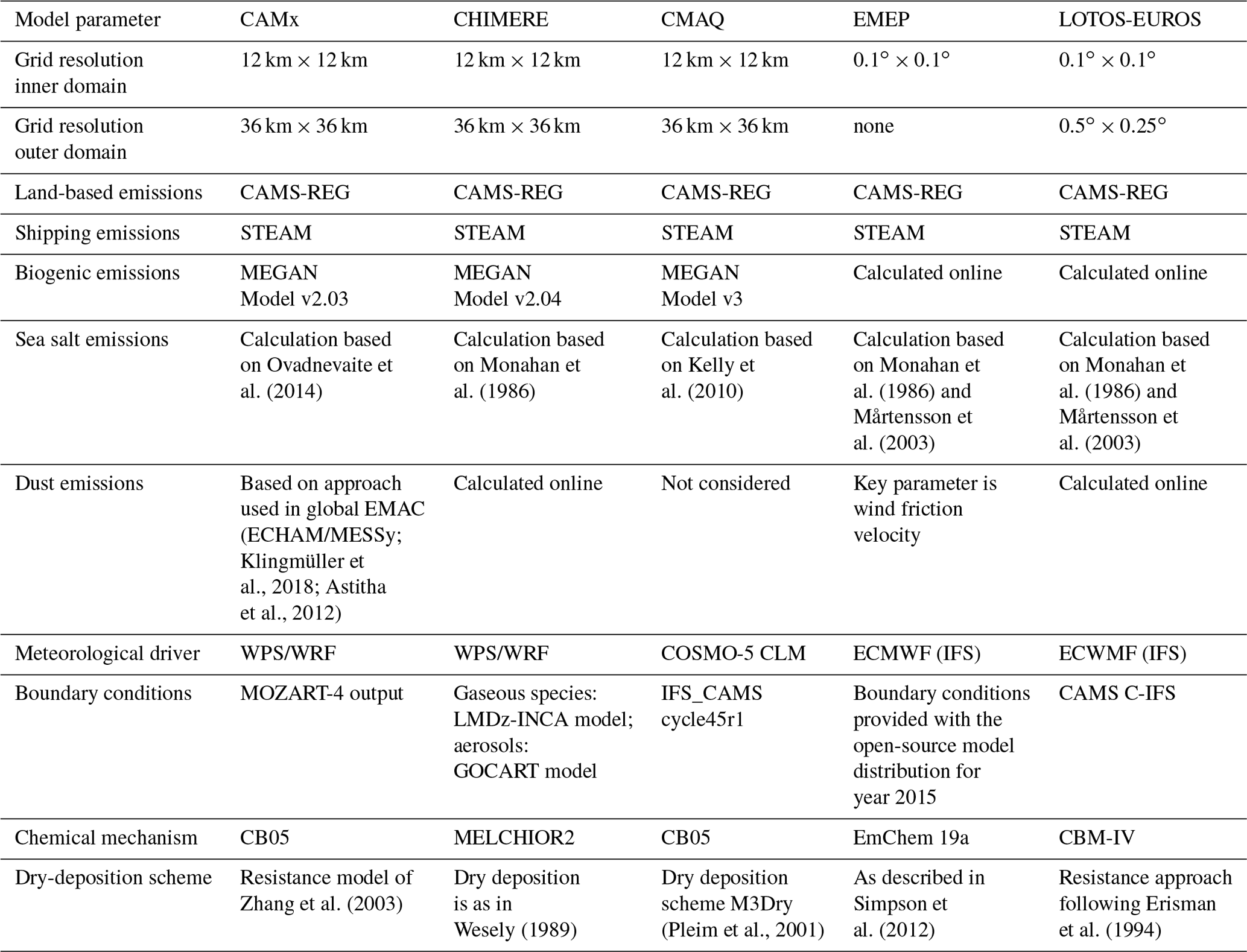
An overview of the input data is shown in Table 1. Input data were the same for shipping emissions using STEAM (version 3.3.0; Jalkanen et al., 2009, 2012; Johansson et al., 2013, 2017), land-based emissions (CAMS-REG, v2.0) and projection (WGS84_lonlat), domain (Mediterranean Sea), resolution (, 12 km × 12 km) and the modeled year (2015). Input data were different for meteorological input data and boundary and initial conditions because the CTMs used their standard setup.
Table 1Main model parameters and input data for the five chemical transport models.
The model simulation runs should all contain NO2 and O3 in grams per cubic meter at an hourly resolution on a 2-D grid from the lowest layer and be provided as a netcdf file following CF conventions. The lowest layer on the ground was used in the present study.
With all CTMs, a reference run for the current air quality situation was performed, including all emissions (base case). Furthermore, all models did one run without the emissions from shipping (no-ship case). The difference between the calculations with all emissions and the calculation without shipping emissions is used to determine the potential impacts of ships on the ambient pollutant concentration. This method shows the change in an emission reduction and the maximal effect, by having a complete switch-off from shipping activity in the no-ship run. Thus, it is referred to as the zero-out method. This was done for all five models.
2.1.1 Model description CAMx
CAMx (Comprehensive Air Quality Model with Extensions) is an Eulerian photochemical dispersion model developed by Ramboll Environ. Version CAMx v6.50 of the model was used in the present study.
For this study, a first domain with a 36 km resolution was defined at the European scale. A second nested domain was defined and named MEDI12 (147×249 points), which covered the center of Europe with a resolution of 12 km. Both meteorological and chemical transport simulations were provided for these domains. WRFv3.9 was run for the simulation of meteorological conditions with 28 vertical layers up to 50 hPa, with FNL data for initial conditions.
For the CAMx simulation, boundary conditions from MOZART-4 were used.
Sea salt emissions are calculated in the SEASALT pre-processor of CAMx. This program generates aerosol emissions of sodium, sulfate and chloride and gaseous emissions of chlorine using CAMx-ready meteorological and land use files. The sea salt emissions program calculates the flux of sea salt over the open ocean using parameterizations developed by Ovadnevaite et al. (2014). The surf zone aerosol flux is calculated by using the Gong (2003) open-ocean approach with an assumed 100 % whitecap coverage. Biogenic emissions were calculated separately with MEGANv2.03 (Model of Emissions of Gases and Aerosols from Nature; Guenther et al., 2006) and then included in the land-based emissions. WBDUST pre-processors deliver dust emissions in CAMx and generate gridded windblown dust emissions. The scheme is based on an updated approach used in the global EMAC (ECHAM/MESSy) atmospheric chemistry–climate model (Klingmüller et al., 2018; Astitha et al., 2012). The mechanism for lightning NOx was not activated in CAMx.
The gas phase chemical mechanism is Carbon Bond 5 (CB05), in which the NMVOC emissions are split into 13 species (TERP, ISOP, XYL, TOL, ETOH, MEOH, IOLE, OLE, ETH, ALD2, PAR, ETHA and FORM) and describe approximately 156 reactions. For semivolatile inorganic species (sulfate, nitrate and ammonium), the equilibrium concentration is calculated using the thermodynamic model ISORROPIA (Nenes et al., 1998). Fourteen vertical levels are simulated with a first layer height of approximately 10 m.
2.1.2 Model description CHIMERE
CHIMERE is an offline chemistry transport model developed by LMD-IPSL/CNRS (Menut et al., 2013). The CHIMERE2017r4 version of the model was used in this study.
WRFv3.9 (Weather Research and Forecasting Model) was run for the simulation of meteorological conditions with 28 vertical layers up to 50 hPa, with FNL data for initial conditions.
Concerning the CHIMERE simulation, boundary conditions are monthly mean climatologies taken from the LMDz-INCA model (Laboratoire de Météorologie Dynamique General Circulation Model – INteraction with Chemistry and Aerosols; Schultz et al., 2006) for gaseous species and from the GOCART model (Global zone Chemistry Aerosol Radiation and Transport; Ginoux et al., 2001) for aerosols (desert dust, carbonaceous species and sulfate). Sea salt emissions were calculated as described in Monahan et al. (1986). MEGANv2.04 calculated biogenic emissions (Guenther et al., 2006). MEGAN is run directly by CHIMERE code, and biogenic emissions are just generated before the air quality run. The mineral dust emissions are calculated on-line. The soil is represented by relative percentages of sand, silt and clay with the USGS soil texture (https://www.usgs.gov/, last access: 20 January 2023). The aeolian roughness length used in CHIMERE is the GARLAP (Global Aeolian Roughness Lengths from ASCAT and PARASOL) dataset as in Prigent et al. (2012). There is no treatment of NOx lightning in CHIMERE.
The gas phase chemical mechanism is MELCHIOR2 (Modele Lagrangien de Chimie de l'Ozone a l'echelle Regionale), in which the NMVOC emissions are split into 10 species (C2H6, NC4H10, C2H4, C3H6, C5H8, OXYL, HCHO, CH3CHO, CH3COE and APINEN) and describe approximately 120 reactions. For semivolatile inorganic species (sulfate, nitrate and ammonium), the equilibrium concentration is calculated using the thermodynamic model ISORROPIA (Nenes et al., 1998). Nine vertical levels are selected with a first layer height at 20 to 25 m.
2.1.3 Model description CMAQ
On the basis of emission input data, the CMAQ Model v5.2 with the AERO6 model calculates air concentration as well as deposition fluxes of atmospheric gases and aerosols (Byun and Schere, 2006; Appel et al., 2017). Atmospheric chemistry is used by the chemical Carbon Bond 5 (CB05) mechanism (Sarwar et al., 2008) cb05tucl with updated toluene chemistry (Whitten et al., 2010), including the chlorine chemistry extension (CB05-TUCL; https://www.airqualitymodeling.org/index.php/CMAQv5.0_Chemistry_ Notes, last access: 20 January 2023). The aerosol scheme AERO6 is used for the formation of secondary inorganic aerosols. Sulfuric acid (H2SO4), nitric acid (HNO3), hydrochloric acid (HCl) and ammonia (NH3) gas-phase–aerosol partition equilibria are solved by the ISORROPIA mechanism (Fountoukis and Nenes, 2007; Nenes et al., 1998). Contained within is the formation of secondary organic aerosol (SOA) from isoprene, terpenes, benzene, toluene, xylene and alkanes (Carlton et al., 2010; Pye and Pouliot, 2012).
Sea salt emissions were calculated as described in Kelly et al. (2010). Biogenic emissions (NMVOC from vegetation and soil NO) were calculated previously with MEGANv3 (Guenther et al., 2012) and then included in the land-based emissions. Emissions of windblown dust were not considered. CMAQ models 30 vertical layers, with the lowest layer from 0 to 42 m and the second layer from 42 to 85 m. The NOx lightning treatment in CMAQ was not activated for the present study.
The COSMO model simulated the meteorological data for CMAQ, applying the version COSMO5-CLM16 (Schultze and Rockel, 2018; Petrik et al., 2021). The MCIP (Meteorology-Chemistry Interface Processor) processed meteorological model output into the input format required for CMAQ. The vertical resolution of the meteorological model was 40 terrain-following geometric height levels up to 22 km. The boundary condition driver used was IFS-CAMS cycle45r1 (Integrated Forecasting System – Copernicus Atmosphere Monitoring Service; Inness et al., 2019) with a vertical resolution of 60 sigma levels up to 65 km.
To prevent the effects from initial conditions on the simulated atmospheric concentrations in 2015, the model run started with a spinup run in mid-December 2014. The grid size of the Mediterranean Sea domain was 12 km × 12 km, nested in a 36 km × 36 km domain covering all of Europe.
2.1.4 Model description EMEP
The EMEP MSC-W (European Monitoring and Evaluation Programme, Meteorological Synthesizing Centre – West, https://www.emep.int/mscw/index.html, last access: 20 January 2023) model is a limited-area, terrain-following hybrid coordinate model designed to calculate air concentrations and deposition fields for major acidifying and eutrophying pollutants, photooxidants and particulate matter (Simpson et al., 2012, 2020).
In this study, a resolution grid on a long–lat projection and with 20 vertical levels was used. The meteorological input data are based on forecast experiment runs with the Integrated Forecast System (IFS), a global operational forecasting model from the European Centre for Medium-Range Weather Forecasts (ECMWF). The meteorological fields are retrieved on long–lat coordinates. Vertically, the fields on 60 eta (η) levels from the IFS model are interpolated onto the 20 EMEP eta levels.
The model version used was rv4.34 with chemical mechanism EmChem 19a (Simpson et al., 2012, 2020). The mechanism builds on surrogate VOC species (Simpson et al., 2012; extended with benzene and toluene) and has 171 gas phase and heterogeneous reactions. The model always assumes equilibrium between the gas and aerosol phases using the MARS equilibrium module (Model for an Aerosol Reacting System) of Binkowski and Shankar (1995). For secondary organic aerosol (SOA), a so-called volatility basis set (VBS) approach (Robinson et al., 2007; Donahue et al., 2009; Bergström et al., 2012) is used. All primary organic aerosol (POA) emissions are treated as nonvolatile to keep emission totals of both PM and VOC components the same as in the official emission inventories, while the semivolatile ASOA and BSOA species are assumed to oxidize (age) in the atmosphere by OH reactions (Simpson et al., 2012).
The generation of sea salt aerosol over oceans is driven by the surface wind, and the EMEP model's parameterization scheme for calculating sea salt generation is based on two source functions: those of Monahan et al. (1986) and Mårtensson et al. (2003). The following natural emissions are calculated in the model for each grid cell and at every model time step: biogenic emissions of isoprene and monoterpenes use near-surface air temperature and photosynthetically active radiation. Soil NO emissions from soils of seminatural ecosystems are specified as a function of N deposition and temperature. The key parameter driving dust emissions is wind friction velocity. Additionally, daily emissions from forest and vegetation fires are taken from the “Fire INventory from NCAR version 1.0” (FINNv1; Wiedinmyer et al., 2011). Emissions of NOx from lightning are included as monthly averages of global 3-D fields on a T21 () resolution (Köhler et al., 1997). For this study, the initial and boundary conditions provided with the open-source model distribution for 2015 were used.
2.1.5 Model description LOTOS-EUROS
LOTOS-EUROS is an Eulerian chemistry transport model (Manders et al., 2017). The model simulates air pollution in the lower troposphere and is of intermediate complexity, allowing ensemble-based simulations and assimilation studies. LOTOS-EUROS performs hourly model output using ECMWF (European Centre for Medium-Range Weather Forecasts) meteorological data. The gas phase chemistry follows the TNO CBM-IV scheme (Schaap et al., 2008).
For sea salt two parametrizations are used for online calculation of emissions: Mårtensson et al. (2003) for fine particles and Monahan et al. (1986) for coarse particles. Biogenic emissions are calculated online during the CTM run. For isoprene, a tree-species-dependent emission factor was used (Schaap et al., 2008; Beltman et al., 2013). NO emissions from soil were calculated as in Novak and Pierce (1993). Dust emissions are also calculated online for three sources of dust. Desert dust follows Mokhtari et al. (2012), and road resuspension and dust from agricultural processes follow a module developed by Schaap et al. (2008). There is no treatment of NOx lightning in LOTOS-EUROS.
LOTOS-EUROS has a dynamical vertical layer structure with five layers in total. The first layer is at 25 m, while the second layer follows the meteorological boundary layer. On top of that, two evenly distributed reservoir layers are defined: one up to 3500 m and one top layer up to 5000 m above sea level. The model has participated in multiple model intercomparison studies (Bessagnet et al., 2016; Colette et al., 2017), showing overall good performance.
2.2 Model domains and nesting
The domain for the intercomparison of a section of the Mediterranean Sea covered a spatial extent from a longitude of −0.95 to 29.95∘ and a latitude of 33.8 to 44.95∘. The grid cell size used was 12 km × 12 km interpolated on a grid nested in a larger 36 km × 36 km grid (except EMEP) covering all of Europe, as shown in Fig. 1. Computational domains of the CTMs can be found in Table S1 in the Supplement.
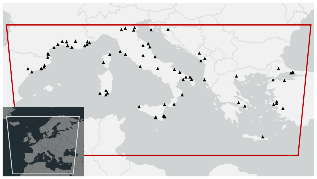
Figure 1Domains and measurement stations. Red trapeze displays the 12 km × 12 km domain; black triangles are locations of measurement stations. At the bottom left, the larger 36 km × 36 km domain is displayed.
2.3 Emissions
2.3.1 Land-based emissions
Annual anthropogenic land-based gridded emissions for 2015 obtained from the CAMS-REG v2.2 emission inventory were used as input by all five compared models. Gridded emission files contain GNFR (Gridded Nomenclature for Reporting) emission sectors for each country for the air pollutants NOx, SO2, NMVOC, NH3, CO, PM10, PM2.5 and CH4. The emissions are provided at a spatial resolution of in longitude and latitude (i.e., ∼6 km × 6 km over central Europe).
The height distribution of emissions per GNFR sector was determined as described in Bieser et al. (2011b). The temporal distribution was determined by separating the annual emissions of each sector into hourly emission data with data splitting as described in Granier et al. (2019). PM was split as described in Bieser et al. (2011a); NOx was split according to Manders-Groot et al. (2016). NMVOC emissions were given for different sectors, using the GNFR, and were separated country-wise. This split was used as provided in the CAMS-REG v2.2 emission inventory (Granier et al., 2019). The species were afterwards split within each CTM according to their chemical mechanism. Information on biogenic emission totals for the whole model domain can be found in Table S20.
2.3.2 Shipping emissions
The shipping emission dataset produced with the STEAM model has a spatial resolution of 12 km × 12 km and a temporal resolution of 1 h. The STEAM emissions are divided into two vertical layers (0 to 36 m; 36 to 1000 m) and are provided for mineral ash, carbon monoxide (CO), carbon dioxide (CO2), elemental carbon (EC), NOx, organic carbon (OC), PM2.5, particle number count (PNC), sulfate (SO4), SOx (containing SO2 and SO3) and VOC. To reduce the number of generated emission maps and the computational resources needed to run the STEAM model, VOC emissions were divided into four categories based on how their emission factors change as a function of the engine load. Emissions of individual VOC species were calculated afterwards based on their mass fractions of the total emissions in the VOC group. Emission factors for VOC are based on the average values taken from various publications (Agrawal et al., 2008, 2010; Sippula et al., 2014; Reichle et al., 2015).
In CAMx, all shipping emissions are put in the first layer. For CHIMERE, all shipping emissions above 36 m and 88 % of the emissions below 36 m have been added to the second layer. Only 12 % of the emissions below 36 m were emitted in the first layer of the model. This was calculated based on the STEAM emission dataset and the stack heights contained therein. Additionally, in CMAQ, shipping emissions were distributed in the two lowest layers, emissions below 36 m were attributed to the lowest layer, and emissions above 36 m were in the second layer. For EMEP simulations, the STEAM emissions were summed from hourly to daily emissions and attributed to the lowest layer (up to 90 m). In LOTOS-EUROS, ∼70 % of emissions below 36 m are assigned to the first layer, which is 25 m thick, and ∼30 % to the second layer. Emissions above 36 m are divided over different height classes: 30 % between 36 and 90 m, 30 % between 90 and 170 m, 30 % between 170 to 310 m, and 10 % between 310 cm and 470 m. Due to the dynamic second model layer (following the meteorological boundary layer), those emissions are put in the second and/or third model layer. In the case of a well-mixed and vertically extended meteorological boundary layer (above 470 m), all emissions are in this second layer, whereas when the boundary layer is shallow, some emissions are put in the third layer.
2.4 Deposition mechanisms
Deposition velocities for gaseous species in CHIMERE, CMAQ and LOTOS-EUROS are based on the formula introduced by Wesely (1989). This formula is the reciprocal sum of aerodynamic resistance (Ra), quasi-laminar sublayer resistance (Rb) and surface resistance (Rc). Nevertheless, all models differ in calculating the single variables. Ra depends on meteorology and surface roughness, which is model dependent. Rb is determined by the friction velocity, depending on the surface type. Rc is the bulk surface resistance, containing different components, i.e., leaf stomata, soil, leaf litter, etc. All of these components use input data that are unique for each model.
In CHIMERE, Rb is estimated following Hicks et al. (1987). The resistance Rc formulation follows Erisman et al. (1994) and the developments made in the EMEP model (Emberson et al., 2000; Simpson et al., 2003, 2012). It uses a variety of additional resistances, mostly to account for stomatal and surface processes, both of which depend on the land use type and season. In CMAQ, the m3dry mechanism was used, which takes Ra and Rb from the provided meteorological data. Rc is calculated in CMAQ as described in Pleim and Ran (2011).
In EMEP quasi-laminar layer resistance Rb follows Hicks et al. (1987). Surface (or canopy) resistance, Rc, is the most complex variable in the deposition model, the calculation of which is described in Simpson et al. (2012). The resistance Rb in LOTOS-EUROS is described following the EDACS system (Erisman et al., 1994). In van Zanten et al. (2010), the parametrizations of different resistances Rc that contribute to resistance for dry deposition of NO2 and O3 are described, depending on land use type. The Deposition of Acidifying Compounds (DEPAC) 3.11 module was used in LOTOS-EUROS, following the resistance approach (van Zanten et al., 2010; Wichink Kruit et al., 2012).
CAMx uses the gas resistance model of Zhang et al. (2003), which is very similar to the Wesely formulations with regard to Ra and Rb. However, the Rc is expressed as several more serial and parallel resistances, based on Wesely (1989), but with some adjustments within CAMx (Ramboll Environment and Health, 2020).
2.5 Observational data, statistical analysis and model results
Model results for total surface concentrations of NO2 and O3 from the five CTMs are evaluated against available measurements of the air quality monitoring network taken from the download service of air quality of the European Environment Agency EEA (https://discomap.eea.europa.eu/map/fme/AirQualityExport.htm, last access: 20 January 2023). NO2 concentrations are monitored at 62 and O3 at 48 background stations. Figure 1 shows the locations of the measurement stations and detailed information on the stations is given in Appendix B.
The criteria for the selection of the stations were as follows: (i) station type is “background”, (ii) elevation is below 1000 m, and (iii) data for more than one of the pollutants NO2, O3 or PM2.5 are available. The PM2.5 measurements were chosen for further evaluation in this intercomparison project. Preferably, stations close to the sea were chosen since simulating potential ship impacts was the major focus of this study. There was no exact threshold for the distance to the coastline assumed, but preferably stations at a distance <30 km from the coast were chosen. Some stations further inland were chosen to check the model performance. Furthermore, the domain was divided into four parts (“west”, “north”, “south”, “east”), and a roughly equal number of stations should be in each parcel (map in Fig. S2). The measured concentrations at the stations were compared to the results of simulations of the CTMs. For this purpose, the grid cell of the respective monitoring station was determined, and modeled concentrations were taken from there.
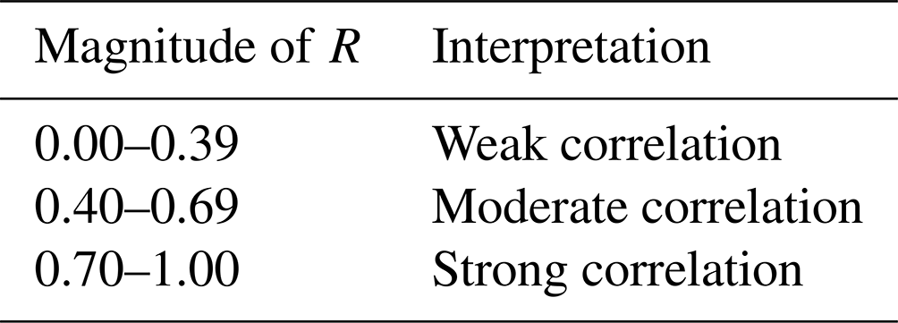
To quantify the CTMs performance, the root mean square error in the modeled values (RMSE), normalized mean bias (NMB) and Spearman's correlation coefficient (R) were calculated for each monitoring station, as described in Appendix A. A categorization for correlation was performed as described in Schober et al. (2018), adjusted and displayed in Table 2.
Table 2Interpretation of the correlation coefficient (R), as described in Schober et al. (2018) (adjusted).
Time series were used to compare the modeled daily mean concentrations to observations at exemplary stations. In addition, the annual mean ship impact was calculated based on hourly data. For a graphical comparison of the model performances R, NMB and RMSE, boxplots were used based on annual values calculated from hourly data at each station. For the intercomparison spatial distribution, annual mean values based on the hourly data are used. The correlation R between models was calculated for each grid cell based on hourly data.
In the following section, the results for NO2 and O3 model performance and spatial distribution will be shown. Afterward, Ox and NOx will be displayed for a more detailed investigation of the photochemistry and lifetime of the species. The results of dry deposition of NO2 and O3 will be considered in Sect. 3.4.
3.1 Model performance and intercomparison
To evaluate the performance of the CTMs, simulated concentrations considering all emission sectors (base case) for annual values of 2015 were compared to actual measured data of NO2 and O3. Based on the results of the five models for the cases with (base case) and without shipping emissions (no-ship case), potential impacts of the shipping sector on the NO2 and O3 concentrations were estimated. Figures of spatial distribution display the annual mean values for 2015 and the potential relative ship impacts. With this setup, the model performance and potential ship impact of the different models can be directly compared.
3.1.1 NO2 model performance
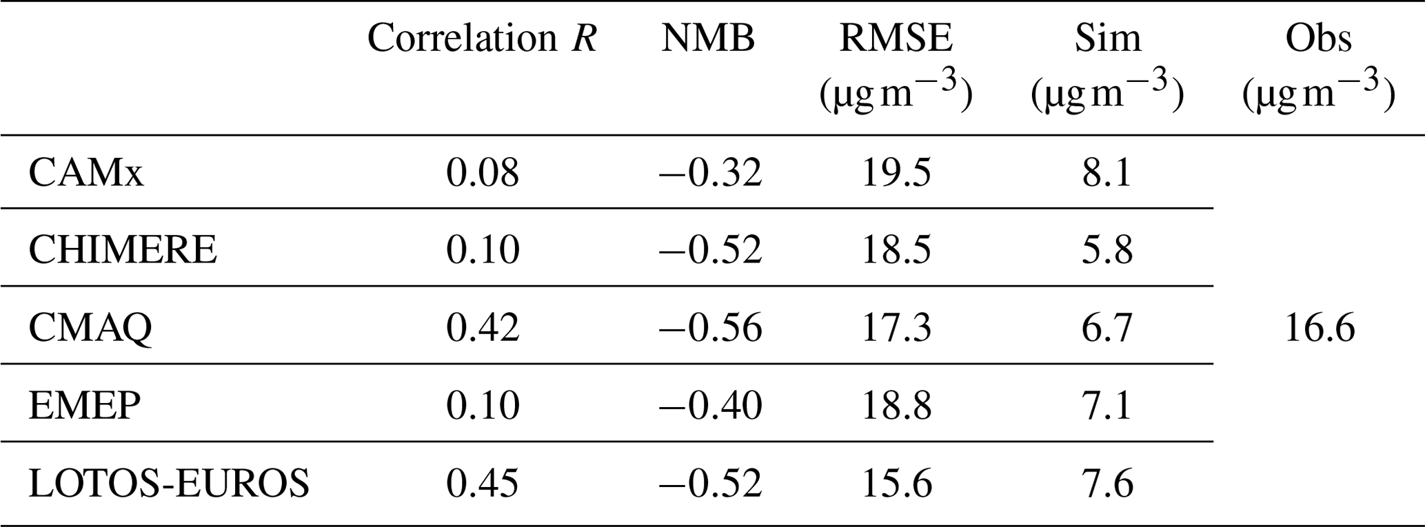
Table 2 contains R, NMB and RMSE based on the annual time series for NO2 at all stations. The highest correlation across all 62 stations showed LOTOS-EUROS followed by CMAQ with a slightly lower correlation (LOTOS-EUROS: R=0.45; CMAQ: R=0.42), whereas for CHIMERE, EMEP and CAMx, non-existent to weak correlation was found (R=0.08 to R=0.10). The NMB suggests that all five CTMs underestimate the annual mean concentrations at most measurement sites; the NMB for all stations is negative for all models. The RMSE is within the same range for all models (RMSE =15.6 to 19.5 µg m−3; Table 3).
Table 3Correlation, normalized mean bias (NMB), root mean square error (RMSE), and observational (obs) and simulated (sim) mean values of NO2 for 2015: first data were averaged station-wise and then averaged for all 62 stations.
Time series for three example stations show the temporal variations between measured and modeled data (Appendix C). The supplements provide an overview of the mean values of stations in each map parcel (west, north, south, east; Fig. S2). Figure C1 displays a time series at an urban background station in France (fr08614, “Gauzy”; lat 43.8344, long 4.374219), which was chosen because southern France will be investigated in greater detail as part of this study. Figure C2 shows a rural background station in Italy (it1773a, “Genga – Parco Gola della Rossa”; lat 43.46806, long 12.95222), which was chosen due to its central location in the domain and the high number of stations in Italy. Figure C3 displays the time series at a station in Greece (gr0035a, “Lykovrysi”; lat 38.06963, long 23.77689) to include a station in the eastern part of the domain.
Measurements at the French station show the highest NO2 values in winter, with peaks between 40 and 55 µg m−3 (Fig. C1). LOTOS-EUROS and EMEP underestimate the values throughout the year. Moderate correlation was calculated for CMAQ (R=0.6) and LOTOS-EUROS (R=0.65) at this station. The simulated ship impact has annual mean values from 0.2 µg m−3 (EMEP, CAMx) to 0.6 µg m−3 (CMAQ) at station fr08614. Shipping emissions have a potential relative impact between 1.8 % (EMEP) and 6.7 % (CMAQ) on the total concentration in the annual mean. The highest potential ship impact at this station was modeled by CMAQ. At the Italian station, it1773a lower NO2 concentrations were measured compared to the station in France. The highest peaks are approximately 20 µg m−3 in winter. At station it1773a, the potential ship impact on the total NO2 concentration has annual mean values between 0.07 µg m−3 (LOTOS-EUROS) and 0.5 µg m−3 (CAMx). The highest relative potential ship impact was 7.9 % and was modeled by CAMx. At station gr0035a, the lowest simulated values are shown by CMAQ and LOTOS-EUROS. The highest values display EMEP at this station, also with the highest correlation between measured and simulated data (R=0.55). The potential ship impact at the Greek station is between 5.0 % (EMEP) and 15.3 % (CAMx), which is higher than the potential ship impact at the other two stations.
All CTMs underestimate the actual measured total NO2 values at both stations, except for LOTOS-EUROS in Italy. None of the models is able to model matching peak values. Neither at the station in France, Italy nor Greece did models show seasonal variation in concentrations, whereas NO2 usually has higher values in winter and lower values in summer, mainly because of lower photolytical degradation and suppressed vertical mixing, as described, e.g., in Ordóñez (2006).
Differences in potential ship impacts between the stations are caused by the location and station type (fr08614: urban background; it1773a: rural background; gr0035a: suburban background). At the French station, the traffic-related NO2 concentration might supersede the ship-related NO2. The station in Italy is not located in a city, so the NO2 concentration caused by ships comes to the fore. The highest potential ship impact was simulated at the station in Greece because it is suburban but close to the Port of Piraeus, which is one of the largest ports in the Mediterranean Sea. As expected, the average potential ship impact is low at stations that are not directly located on the coast or near a harbor.
To compare the correlation R, NMB and RMSE at all measurement stations for all models, the results of the comparison are divided by country and displayed in boxplots (Fig. 2). Each dot displays one measurement station. The correlation measured against the simulated annual mean NO2 is highest for LOTOS-EUROS and CMAQ in all countries, reflecting the results shown in Table 3 for correlation. Nevertheless, boxplots for NMB and, in particular, for RMSE show that differences among countries are larger than differences among the models (Fig. 2b, c). This means that all models show good or bad performance at some stations, which was not found to be statistically relevant.
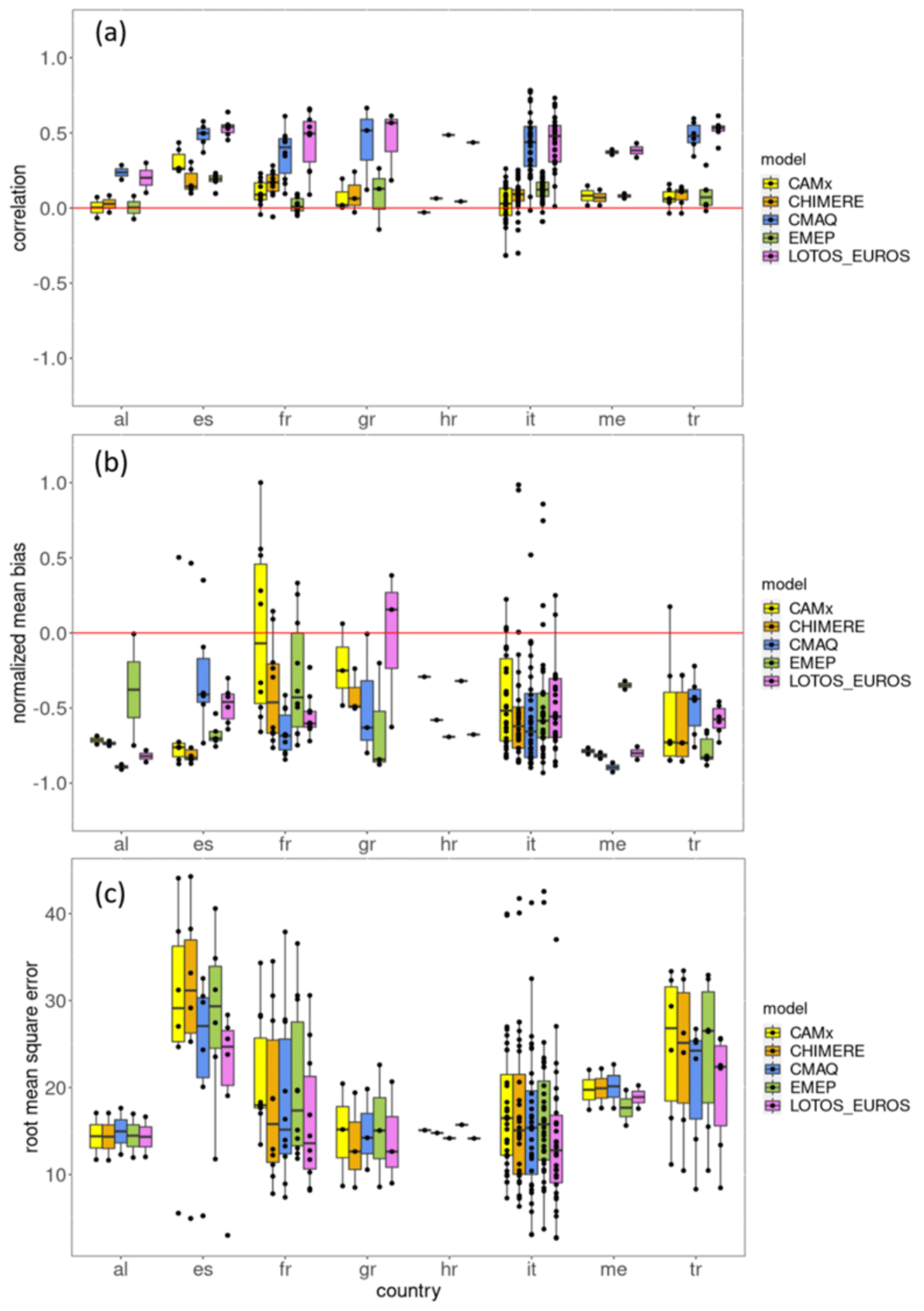
Figure 2(a) Correlation, (b) NMB and (c) RMSE for annual mean NO2 concentration based on hourly data. Dots display annual mean values at measurement stations for the respective countries (al: Albania; es: Spain; fr: France; gr: Greece; hr: Croatia; it: Italy; me: Montenegro; tr: Turkey). Boxplots are for the models with the boxes displaying the interquantile range (IQR) between the 25th (Q1) and 75th (Q3) percentile, the black line displays the median (Q2), and whiskers are calculated as Q1 (minimum) and Q3 (maximum).
Underestimations by models of NO2 at urban sites were found in other studies (Karl et al., 2019b; Giordano et al., 2015), despite differences in grid size. Karl et al. (2019b) used a grid resolution of 4 km, and Giordano et al. (2015) used a grid resolution of ∼0.25∘ (27 to 28 km). The underestimation might be due to too low emissions in the inventory used by the models and the heterogeneity of emissions. Regional CTMs cannot display small-scale spatial heterogeneity; coarse grid cells are not representative of the measurement location. Giordano et al. (2015) suggested in their study that the underestimation of NO2 could be caused by either an underestimation of the chemical lifetime of NOx, excessively high dry deposition, an underestimation of natural emissions at rural and remote stations, or a combination of these factors. Differences in radical concentrations and reactive nitrogen might be additional reasons for underestimation (Knote et al., 2015).
The model performance of NO2 has shown that differences in time series between the models occur, caused by the differences in meteorology and large grid size. Large grid sizes can cause errors insofar as, in simulations, the land areas are not seen as such but as water areas. This is especially problematic when having measurement stations located close to the sea.
3.1.2 NO2 spatial distribution
The simulated annual mean NO2 concentrations considering all emission sectors are similar for all CTMs, with a median ensemble mean of ∼2.5 µg m−3 (Fig. 3a). Regarding the spatial distribution CAMx and CHIMERE have the largest areas, with values exceeding 5.0 µg m−3, especially along the main shipping routes and in urban areas (Fig. 4). The CMAQ, EMEP and LOTOS-EUROS figures look similar, which is in good agreement with the displayed time series in Sect. 3.1, where the results are within the same range.
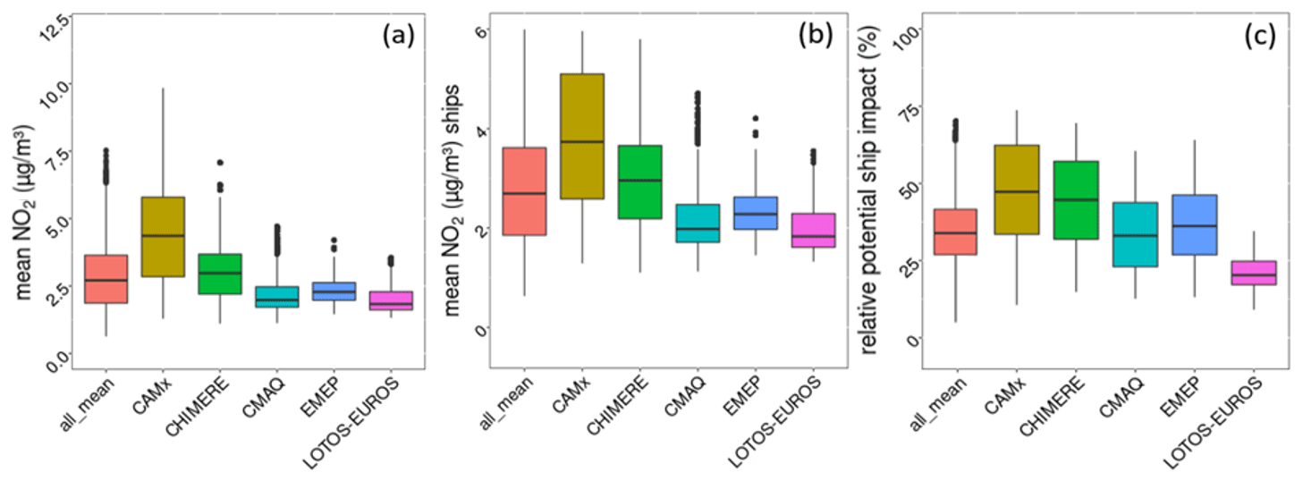
Figure 3Annual mean for all grid cells in the whole model domain. (a) Mean NO2 for all emission sectors (base case); (b) mean NO2 for shipping only; (c) relative potential ship impact on total NO2 concentration. All_mean is the mean value of all models, with a median of (a) 2.8 µg m−3, (b) 0.7 µg m−3 and (c) 27.7 µg m−3.
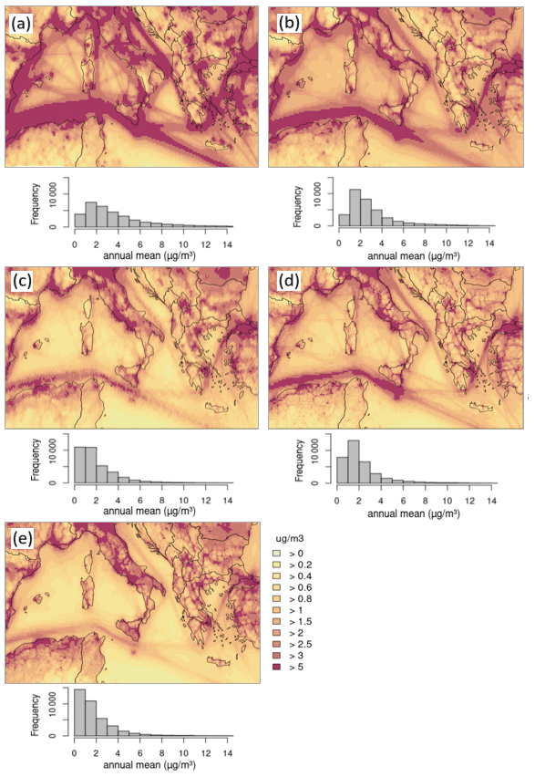
Figure 4Annual mean NO2 total concentration. (a) CAMx; (b) CHIMERE; (c) CMAQ; (d) EMEP; (e) LOTOS-EUROS. Below the domain figure the respective frequency distribution is displayed for the annual mean NO2 concentration, referring to the whole model domain.
Over land area, all model simulations display a concentration pattern ranging within 1 order of magnitude. Nevertheless, the frequency distributions of the CMAQ, EMEP and LOTOS-EUROS simulations show the highest frequency between 1.0 and 2.0 µg m−3, whereas for CAMx and CHIMERE, they are more equally distributed. Higher values of NO2 concentrations simulated by CAMx and CHIMERE might indicate a longer lifetime of NO2 in the atmosphere. NO2 reacts quickly with hydroxyl radicals (OH) and forms HNO3, or NO2 photolysis creates O3 during the daytime. The annual mean HNO3 concentrations are between 2.0 to 5.0 µg m−3 for CAMx and CHIMERE over water areas and are 0.8 to 2.0 µg m−3 over water areas for CMAQ, EMEP and LOTOS-EUROS (Fig. S11). Over land areas, the HNO3 concentrations are within one range for all models. A lower HNO3 concentration is expected for CTMs with a longer lifetime of atmospheric NO2. Nevertheless, there can be a misinterpretation when both concentrations are high. Therefore the data were normalized by using the HNO3:NO2 ratio (Fig. S12). Differences are displayed especially along the main shipping routes. There, values are lower in CAMx and EMEP compared to the other models. This can be explained by the lower HNO3 formation by these models along the shipping routes.
Also the meteorology might influence the vertical mixing of NO2. This leads to differences between the models or explains the similarity between CAMx and CHIMERE due to the use of the same meteorology. Nevertheless, this point will not be discussed here in detail since in the present study only the lowest layer was considered and the vertical mixing processes were not evaluated.
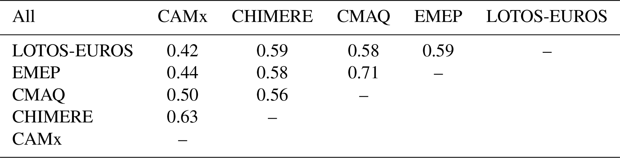
The correlation between the models for total NO2 concentration was calculated based on hourly data (Table 4). The highest correlation was found between CAMx and CHIMERE (R=0.80). Weak correlations were found between LOTOS-EUROS and CAMx (R=0.31) and LOTOS-EUROS and CHIMERE (R=0.36). This weak correlation is due to the differences in frequency distribution, with LOTOS-EUROS showing most values below 1.0 µg m−3, whereas for CAMx and CHIMERE, more values are located in the higher value ranges. Overall, the models can give a robust estimate regarding the base run of the annual mean of NO2.
Table 4Correlation for the NO2 base run between models for the whole domain (all grid cells), based on hourly data for NO2 total concentration.

The highest potential impact of ships on total NO2 concentrations was found on the main shipping routes, with values >85 % (Fig. 5). Similar values were found for the Baltic Sea (Karl et al., 2019b) and for the Iberian Peninsula (Nunes et al., 2020). CHIMERE and CAMx model the highest values over the sea region, with a potential ship impact on NO2 between 60 % and 85 %. CMAQ, LOTOS-EUROS and EMEP have similar patterns for ship impacts over the sea.
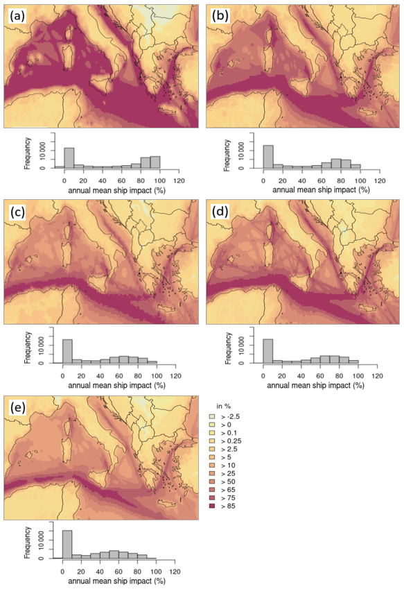
Figure 5Annual mean NO2 potential ship impact. (a) CAMx; (b) CHIMERE; (c) CMAQ; (d) EMEP; (e) LOTOS-EUROS. Below the domain figure the respective frequency distribution is displayed for the annual mean NO2 potential ship impact, referring to the whole model domain.
On the Mediterranean coastline, CMAQ, CHIMERE, LOTOS-EUROS and EMEP simulate a similar potential impact, with 25 % to 45 % potential ship impacts on total NO2. Merico et al. (2017) found similar results in a study with an NO2 shipping impact of up to 32.5 % regarding four port cities in the Adriatic–Ionian Sea. CAMx reveals a higher impact with >85 % at the coastline. The potential ship impact displayed in the time series in Sect. 3.1 was lower, although the measurement stations were not far from the coast. This shows that although the potential impact from ships reaches regions far from the coast, the highest impact is over the sea area. The frequency distribution for the relative ship impact shows that all models simulate the most values between 0 % and 5.0 % of the potential ship impact. Interestingly, the distribution is lowest at values between 20 % and 40 % (CMAQ, EMEP, LOTOS-EUROS) and 60 % (CAMx, CHIMERE) and then increases again at higher values, showing a bimodal distribution. This is due to large areas with high potential impacts over water and large areas with low potential impacts over land or near harbors.
Over land in the northeast area of the domain, slightly negative potential ship impacts are derived from the CMAQ, CAMx, LOTOS-EUROS and EMEP results. CHIMERE shows only very few negative values but in the same region. Negative potential ship impacts on NO2 concentrations may arise when the zero-out method is applied. They are a consequence of the nonlinear NOx gas phase chemistry. Especially in areas where the impact of NOx emissions from shipping is very low, less NO oxidation takes place because the additional NO from shipping in other areas has already consumed the oxidants (e.g., O3).
The boxplots in Fig. 3 display the annual mean values for the whole model domain of NO2. Model results vary for the base run but also for the potential ship impact. This variability needs to be taken into account when the predictive power of CTMs is considered. The “all_mean” boxplot displays the mean of all models and shows that in comparison with other models, CAMx has high values. It further helps to show which CTM tends to simulate higher or lower values compared to others. The all_mean boxplots show similar ranges as boxplots for CMAQ and EMEP, particularly regarding absolute and relative potential ship impacts. Additionally, models simulating a higher overall concentration of pollutants also tend to simulate a higher potential ship impact. The relative potential ship impact is highest for CAMx and CHIMERE and lowest for LOTOS-EUROS.
3.1.3 O3 model performance
The tropospheric O3 concentrations are strongly connected to the NO2 concentration and to the oxidized nitrogen chemistry in the atmosphere. O3 can be both an initiator and a product of photochemistry; thus, it is crucial in tropospheric chemistry.
Simulated versus measured data of 1-year daily mean O3 time series show a weak (EMEP: R=0.38) to moderate correlation (CAMx: R=0.40; CHIMERE: R=0.47; CMAQ: R=0.60; LOTOS-EUROS: R=0.69; Table 5).
Table 5Correlation, normalized mean bias (NMB), root mean square error (RMSE), and observational (obs) and simulated (sim) of O3 as the mean values for 2015: the first data were averaged station-wise and then averaged for all 48 stations.

Selected time series represent these differences in correlation (Appendix D). Nevertheless, for the first months of the year CHIMERE, CAMx and CMAQ overestimate the actual measured O3 values (Fig. D1: station fr08614; Fig. D2: station it1773a; Fig. D3: gr0035a).
During summer months, O3 shows the highest values due to increased photochemical activity. The simulated potential ship impact is between 1.1 µg m−3 (CAMx) and 2.8 µg m−3 (LOTOS-EUROS) at station fr08614 and has a relative potential impact between 1.3 % (CAMx) and 4.0 % (CHIMERE) on the total concentration. At station it1773a, the mean O3 potential ship impact is between 1.0 µg m−3 (CAMx) and 3.0 µg m−3 (CHIMERE), and the relative potential impact ranges from 1.1 % (CAMx) to 3.5 % (LOTOS-EUROS). The potential ship impact of station gr0035s ranges from −0.1 µg m−3 (CAMx) to 3.7 µg m−3 (CMAQ; LOTOS-EUROS), which is a relative potential impact of −0.1 % (CAMx) and 3.7 % (CMAQ).
The O3 potential ship impact is within the same range at both stations and for all five CTMs. Figure 6 shows that CMAQ has the smallest bias compared to the other models (NMB =0.28), followed by LOTOS-EUROS (NMB =0.36). The RMSE is lowest for CMAQ (RMSE =31.2 µg m−3) and LOTOS-EUROS (RMSE =32.6 µg m−3), along with the lower NMB compared to the other models. The performance analysis revealed that all five models predict higher O3 concentrations than those measured at almost all stations (NMB >0). The overestimation of actual measured O3 by the models is in line with results from previous studies (Karl et al., 2019b; Appel et al., 2017; Im et al., 2015a, b). Im et al. (2015a) showed that O3 concentrations above 140 µg m−3 are underestimated, while concentrations below 50 µg m−3 are overestimated by 40 % to 80 % in all considered models. This overestimation of O3 by the models is likely linked to the chemical boundary conditions used in the regional CTMs. Analyses of the boundary conditions revealed that, especially in winter, O3 levels are mostly driven by transport instead of local production due to limited photochemistry (Giordano et al., 2015).
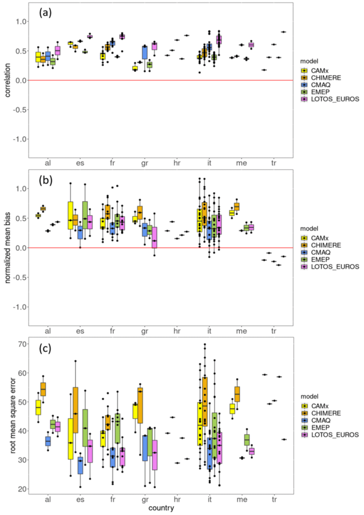
Figure 6(a) Correlation, (b) NMB and (c) RMSE for annual mean O3 concentration. Dots display values at measurement stations for the respective countries (al: Albania; es: Spain; fr: France; gr: Greece; hr: Croatia; it: Italy; me: Montenegro; tr: Turkey). Boxplots are for the models with the boxes displaying the interquantile range (IQR) between the 25th (Q1) and 75th (Q3) percentile, the black line displays the median (Q2), and whiskers are calculated as Q1 (minimum) and Q3 (maximum).
CHIMERE uses boundary conditions from monthly mean climatologies simulated with the LMDz-INCA model, CAMx uses MOZART-4 output, LOTOS-EUROS and CMAQ use IFS-CAMS reanalysis data, and the EMEP model uses ozone boundary conditions provided with the open-source model distribution for 2015. These differences in input for the boundary conditions can be seen as the reason for the varying results in O3 (Figs. S13 to S16).
All CTMs performed relatively well and are able to represent the course of the year, with higher values in summer and lower values in winter. Nevertheless, in some cases, the values in spring are overestimated.
3.1.4 O3 spatial distribution
The annual mean concentration of O3 considering all emission sectors is between 60 and 120 µg m−3 for all models (Fig. 8). This is consistent with the measurements displayed in the time series in Sect. 3.2.1. CHIMERE, CAMx and LOTOS-EUROS show particularly high O3 concentrations over the sea. Interestingly, EMEP results are similarly high over the sea area, but in comparison with other CTMs, concentrations are lower over land, and even values below 60 µg m−3 can be seen in the Po valley (Fig. 8d). Regarding the correlation between the models for total concentration over the whole domain, it is highest between CMAQ and EMEP (R=0.71) and lowest for CAMx and LOTOS-EUROS (R=0.42), but predominantly moderate correlations were found among the models (Table 6).
Table 6Correlation between models for the whole domain (all grid cells) based on hourly data for O3 total concentration.
In general, all CTMs show high annual mean concentrations over the sea areas and low annual mean concentrations over land areas. This is due to lower dry deposition over sea and the overall higher emissions over land. Furthermore, high values of O3 are expected to enter the domain from the eastern part of the Mediterranean Sea. This point will be discussed in Sect. 4. The frequency distribution of the annual mean total concentration of O3 has a bimodal distribution for CHIMERE, CMAQ and EMEP. This reflects photochemical O3 depletion or production, with high values over water areas and lower values over land. Over water, low O3 depletion is expected during the night. A comparison of diurnal cycles of O3 over water and over land shows that this presumption is reflected by CMAQ and EMEP results, showing more pronounced cycles of O3 in grid cells over land (Fig. S17). However, the diurnal cycles of CAMx, CHIMERE and LOTOS-EUROS do not show differences in amplitude over land and water. Despite this, over water, all models show a higher spread of values within diurnal cycles, displaying that there is more variability in the course of the year over water than over land.
The potential relative impact of ships on total O3 concentrations is lowest in areas with a high potential impact of shipping on total NO2 (Fig. 9). It decreases to −20 % in areas with high NO2 concentrations in all model results, displaying a local-scale titration of O3 by NO, which is emitted by ships. This reverse relationship between NO2 and O3 was already shown in other studies (e.g., Karl et al., 2019a). Measurement studies also indicate that emissions of NO lead to local reduction in O3 concentration and showed that there could be an increase at larger distances (Merico et al., 2016). Consequently, the largest areas with O3 destruction for the CAMx and CHIMERE coincide with areas where the models show the highest potential impact of shipping on NO2. The comparison with the time series shows the highest potential ship impact on the total O3 concentration in summer. Likewise, in Sect. 3.1.4 the lowest potential ship impact was found for CAMx.
Figure 7 shows boxplots with annual mean values of the models for the whole domain. It shows that CAMx, CHIMERE and LOTOS-EUROS are within one range regarding the annual mean total concentration. The CMAQ and EMEP simulations are lowest for the annual mean O3 total concentration. Regarding potential ship impact, all CTMs except CAMx are within one range.
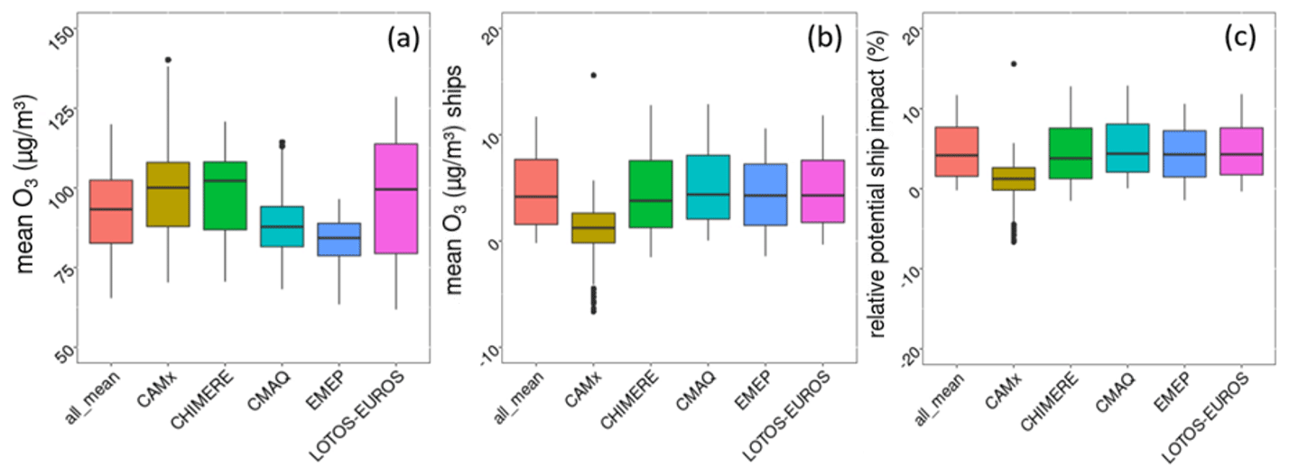
Figure 7Annual mean for the whole model domain. (a) Mean O3 for all emission sectors (base case); (b) mean O3 for shipping only; (c) relative potential ship impact on total O3 concentration. All_mean is the mean value of all models, with a median of (a) 92.4 µg m−3, (b) 4.0 µg m−3 and (c) 4.2 µg m−3.
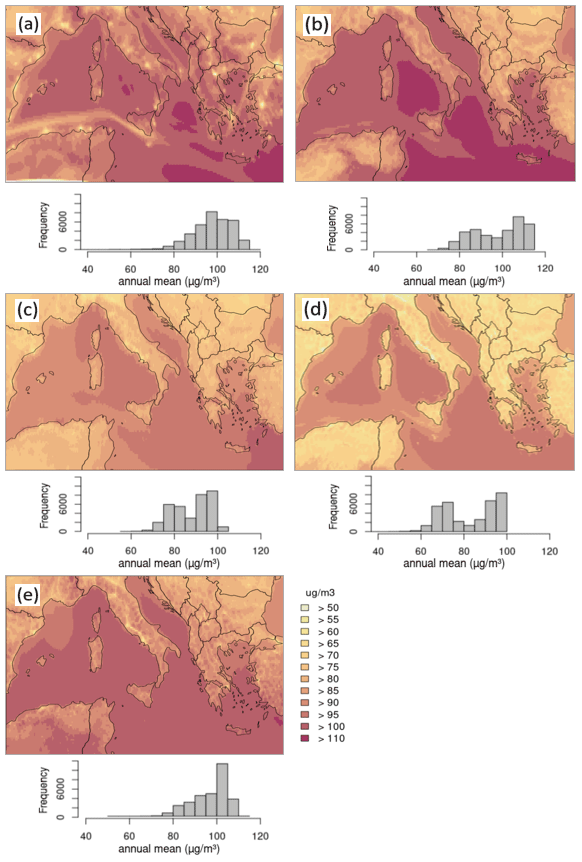
Figure 8Annual mean O3 total concentration. (a) CAMx; (b) CHIMERE; (c) CMAQ; (d) EMEP; (e) LOTOS-EUROS; the panels show the emisbase spatial distribution and the annual mean value, and white areas contain values below 60 µg m−3. Below the domain figure the respective frequency distribution is displayed for the annual mean O3 concentration, referring to the whole model domain.
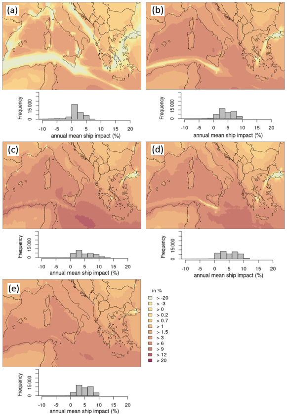
Figure 9Annual mean O3 potential ship impact. (a) CAMx; (b) CHIMERE; (c) CMAQ; (d) EMEP; (e) LOTOS-EUROS; white areas in the panels display values below −20 %. Below the domain figure the respective frequency distribution is displayed for the annual mean O3 potential ship impact, referring to the whole model domain.
The present study does not contain the parts of the Mediterranean Sea furthest east due to the focus of the project on the western Mediterranean Sea with its harbor cities as well as due to the limited extent of the WRF domain. A more detailed investigation of the boundary conditions of CMAQ has shown high O3 values in the eastern part of the domain. A high O3 production over the eastern Mediterranean Sea and a steep west–east gradient of O3 were described in previous studies (i.e., Doche et al., 2014; Safieddine et al., 2014; Liu et al., 2009). This production influences the amount of O3 in the western part of the Mediterranean Sea. Safieddine et al. (2014) found an increase of up to 22 % in O3 in the eastern part of the Mediterranean Basin compared to the middle of the basin. Doche et al. (2014) described a steep west–east O3 gradient with the highest concentrations over the eastern part of the Mediterranean Basin.
Overall, all models showed a relatively good performance for O3 but differed in simulating spatial distribution and potential ship impact mainly over water. Although boxplots for annual mean values of O3 differ, for relative potential ship impact they show that CHIMERE, CMAQ, EMEP and LOTOS-EUROS are within one range. Diurnal cycles did not reveal differences in O3 depletion over water and land among the models.
3.2 Ox spatial distribution
The oxidation of VOCs produces O3 in the troposphere when nitrogen oxides (NO; NO2) and sunlight are present. Central to understanding this production is the photostationary state formed between NO, NO2 and O3 in sunlight. In emission-free air, a steady equilibrium would be expected; nevertheless, emission sources disturb this equilibrium. In areas with high NO emissions, O3 destruction is expected, resulting in lower O3 concentrations along the main shipping routes, in urban areas and in harbor cities.
The results show that all five CTMs tend to underestimate NO2 and overestimate O3 but at different magnitudes. For a better understanding of photochemical air pollution and chemical coupling, the oxidant levels () were calculated and displayed for all emission sources and for the potential ship impact. Clapp and Jenkin (2001) showed that the concentration of Ox levels can be described as an NOx-independent regional impact, where the Ox impact equates to the O3 background, and an NOx-dependent local impact. The NOx-dependent impact correlates with the primary pollution, coming from direct NO2 emissions or VOC, which promote conversion from NO to NO2 (Clapp and Jenkin, 2001).
In comparison with the O3 spatial distribution and frequency distribution, the annual mean concentration of Ox displays a similar pattern between the results (Fig. 10). As was the case for O3, CHIMERE and CAMx show the highest values over the sea area, and EMEP shows the lowest values over land areas. The frequency distribution shows bimodally distributed values for CHIMERE, CMAQ and EMEP, as for O3. Thus, Ox levels are mainly NOx-independent.
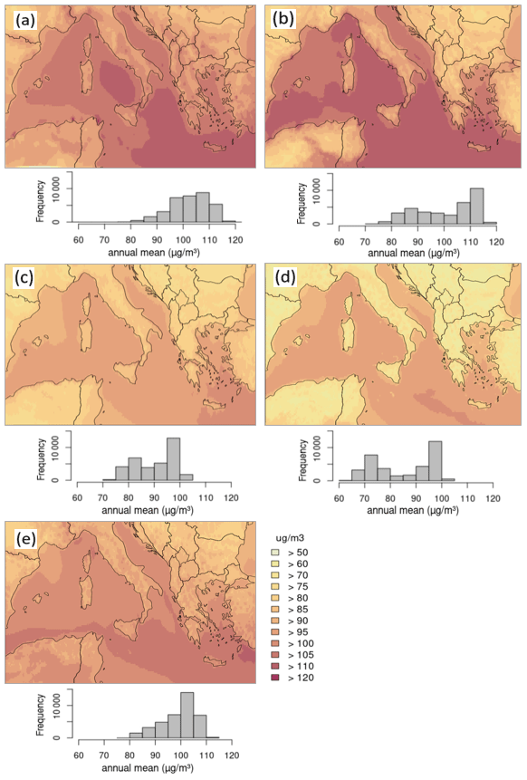
Figure 10Annual mean Ox () concentration. (a) CAMx; (b) CHIMERE; (c) CMAQ; (d) EMEP; (e) LOTOS-EUROS. Below the domain figure the respective frequency distribution is displayed for the annual mean Ox concentration, referring to the whole model domain.
Nevertheless, NOx-dependent Ox formation can also be seen in the potential ship impact on the total Ox concentration (Fig. 11). The relative potential impact of Ox displays how much substances from ships are added to the atmosphere. Ox shows a strong conversion of NO2 and O3; thus the shipping lanes are no longer visible. High Ox potential impacts over water areas for CHIMERE, CMAQ, EMEP and LOTOS-EUROS indicate the local potential impact from shipping emissions (NO2 and VOC), which cause high Ox levels in these areas. For CAMx, the Ox potential impact was lower. This might be traced back to the overall higher concentration of NO2 and O3 in CAMx, leading to a lower proportion of other substances. Also, the differences between the Ox results among the models can occur due to the difference in O3 that in turn results from the input from the boundaries. Here, CAMx displays an overall high input of O3 from the boundary.
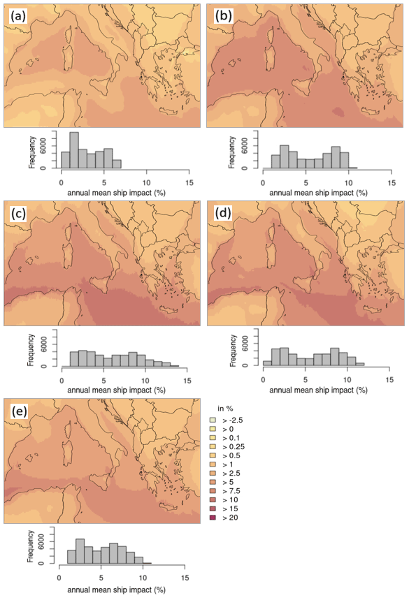
Figure 11Annual mean Ox () potential ship impact. (a) CAMx; (b) CHIMERE; (c) CMAQ; (d) EMEP; (e) LOTOS-EUROS. Below the domain figure the respective frequency distribution is displayed for the annual mean Ox potential ship impact, referring to the whole model domain.
3.3 NOx spatial distribution
To gain further insight into the differences in the lifetime of NO2 in the models, NOx () was calculated and displayed (Appendix E). Differences in NOx provide suggestions regarding the lifetimes because of the reaction of NO2 with OH to HNO3. The latter forms ammonium nitrate aerosol together with ammonia; thus, NO2 is no longer in the gaseous phase. Another explanation is the dry deposition of NO2, which also causes a loss and consequently differences in the NOx pattern due to different deposition mechanisms. The spatial distribution of the annual mean NOx and potential ship impact on the total NOx concentration have shown a very similar pattern as for NO2. The values of CAMx and CHIMERE are within one range, displaying higher values compared to CMAQ, EMEP and LOTOS-EUROS. These three models show results within one range.
To see the chemical fate of NO2 the dry deposition could provide an indication and will be considered in the following Sect. 3.4.
3.4 Dry deposition
In the present study, dry deposition of NO2 and O3 are displayed for the base and the no-ship case for CAMx, CHIMERE, CMAQ and LOTOS-EUROS. EMEP does not deliver separate NO2 and O3 deposition files but does deliver oxidized and reactive nitrogen. Thus, EMEP is not considered in this chapter.
3.4.1 Dry deposition of NO2
The annual mean NO2 dry deposition of all four compared CTMs displays similar values over land areas (Fig. 12). In cities and densely populated regions, all models show high NO2 dry deposition, with values over 300 mg m−2 yr−1. Nevertheless, the frequency distribution of all values shows that this is mainly the case for CAMx and LOTOS-EUROS. Additionally, over the sea, the pattern of annual mean dry deposition of NO2 is also similar for CAMx and LOTOS-EUROS.
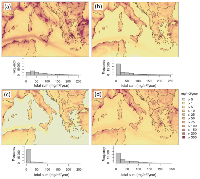
Figure 12Annual total dry deposition of NO2. (a) CAMx; (b) CHIMERE; (c) CMAQ; (d) LOTOS-EUROS. Below the domain figure the respective frequency distribution is displayed for the annual mean NO2 dry deposition, referring to the whole model domain.
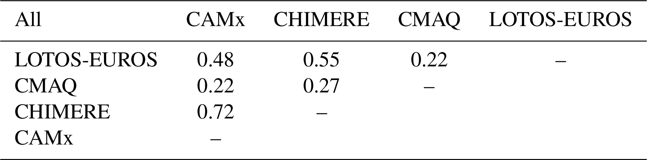
Table 7 shows that the correlation was strongest between CHIMERE and CAMx (R=0.72). Similarities and strong correlations in the output of both models were also found for the NO2 concentration in Sect. 3.1.2. This can be traced back to the same meteorology data that were used by both CTMs.
Table 7Correlation between models for the whole domain (all grid cells) based on daily data for NO2 total dry deposition.
The relative potential ship impact on the annual dry deposition of NO2 is displayed in Fig. 13. The lowest potential ship impact on NO2 dry deposition is simulated by CMAQ and LOTOS-EUROS. In particular, CMAQ shows large areas with negative (−2.5 %) potential ship impacts over land. The CHIMERE simulations looks similar to the CAMx simulations over land. Along the coastline, CMAQ and LOTOS-EUROS show a potential impact of ships between 10 % and 25 %; CAMx and CHIMERE expect a potential ship impact on the total annual deposition of 25 % to 75 %. The highest potential impact is displayed by CAMx.
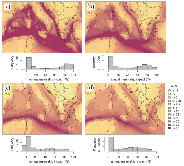
Figure 13Annual mean dry deposition of NO2 relative potential ship impact. (a) CAMx; (b) CHIMERE; (c) CMAQ; (d) LOTOS-EUROS. Below the domain figure the respective frequency distribution is displayed for the annual mean NO2 dry deposition potential ship impact, referring to the whole model domain.
Differences in NO2 dry-deposition model results can be due to the dry-deposition velocities but also due to the different meteorology data used by the models (Wichink Kruit et al., 2014). Dry-deposition velocities of NO2 (Fig. S18) show that deposition velocities of CHMIERE and CMAQ are within one range and are lower compared to CAMx and LOTOS-EUROS deposition velocities. Velocities of the latter two are within one range. High velocities might lead to higher deposition rates, leading to high annual mean deposition. This is reflected in the annual dry deposition of NO2, where CAMx and LOTOS-EUROS simulate the highest values. Overall, the models have more differences in NO2 dry deposition than in air concentration. As was the case for NO2 concentration, CAMx simulated the highest values in dry deposition. The lowest values in NO2 dry deposition are displayed by CMAQ. In addition, the correlation between CMAQ and the other models was lowest.
High NO2 deposition over water areas caused by ships contributes to eutrophication (Vivanco et al., 2018). A study by Im et al. (2013) showed values of approximately 500 kg (N) m−2 yr−1 ( mg m−2 yr−1) over the Mediterranean Sea, which means an exceedance of the critical load of 2 g to 3 g (N) m−2 yr−1 ( 2000 to 3000 mg m−2 yr−1) to marine and coastal habitats (Bobbink and Hettelingh, 2011). The present study focused on NO2 dry deposition; thus, a direct comparison with critical load levels or with other studies regarding total N deposition would not be possible. A subsequent calculation of N showed that the simulated values in the present study do not exceed the critical loads (Appendix F). Nevertheless, NO2 dry deposition from ships contributes to the total N deposition budget, thus increasing with ship traffic and affecting the ecosystems in the Mediterranean Sea.
3.4.2 Dry deposition O3
Dry deposition is a major sink for O3 in the lowest model layer. O3 has high destruction rates on vegetated surfaces through plant stomata and lower rates on surfaces such as water or snow (Clifton et al., 2020). Spatial patterns of annual total O3 dry deposition confirm this distribution. Over sea annual totals are lower (250 to 1000 mg m−2 yr−1) compared to values over land (2500 to 10 000 mg m−2 yr−1; Fig. 14). The correlation for the annual total concentration of O3 dry deposition is highest between CHIMERE and CAMx, showing a moderate correlation (R=0.57; Table 8).
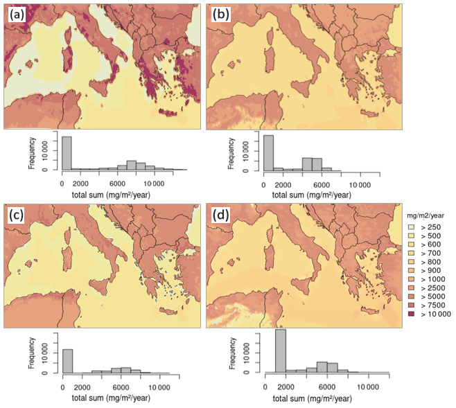
Figure 14Annual total dry deposition of O3. (a) CAMx; (b) CHIMERE; (c) CMAQ; (d) LOTOS-EUROS. Below the domain figure the respective frequency distribution is displayed for the annual mean O3 dry deposition, referring to the whole model domain.
Table 8Correlation between models for the whole domain (all grid cells) based on daily data for O3 total dry deposition.

Figure 15 shows the potential ship impact on the total dry deposition of O3. CMAQ and LOTOS-EUROS are within a similar range, with potential impacts of ships of 5 % to 10 % over water surfaces. The lowest potential impact of −5 % in the main shipping lanes is simulated by CAMx, showing a similar pattern as for the O3 potential ship impact. Over land areas, ships contribute to dry O3 deposition from 0.25 % to 2.5 %.
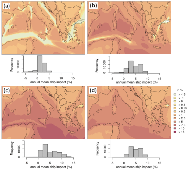
Figure 15Annual mean dry deposition of O3 relative potential ship impact. (a) CAMx; (b) CHIMERE; (c) CMAQ; (d) LOTOS-EUROS. Below the domain figure the respective frequency distribution is displayed for the annual mean O3 dry-deposition potential ship impact, referring to the whole model domain.
In addition to the impact of O3 dry deposition on plant stomata, it is important to explain differences in surface O3 concentration results. The O3 concentration is sensitive to the deposition velocity (Clifton et al., 2020), which differs among the four CTMs. This can be confirmed by studies comparing deposition schemes, where differences in O3 concentration between models are caused by the variety of processes (Clifton et al., 2020). In particular, the variability in deposition velocities across models, as discussed in Sect. 3.3.1, is seen as an originator leading to uncertainties in tropospheric O3 (Wild, 2007). Deposition velocities for the models in the present study (Fig. S19) show the lowest velocities for CMAQ. Highest velocities were found for CAMx over land areas. The deposition velocities go along with the annual dry deposition, with high velocities in areas with high dry deposition.
A model comparison study with 15 models by Hardacre et al. (2015) found the greatest differences in total O3 dry deposition occurring in areas where deposition velocities and O3 concentrations are highest. Additionally, soil moisture has an important impact on O3 deposition and concentration. An evaluation study within the CHIMERE model found that especially in southern Europe, where soil is close to the wilting point during summer and affects stomatal opening, O3 dry deposition declines (Anav et al., 2018). This in turn affects the concentration of gases in the lower atmosphere and thus has an impact on O3 concentrations.
The potential impact of ships on air pollution by NO2 and O3 the Mediterranean Sea region was simulated with five different regional-scale CTMs (CAMx, CHIMERE, CMAQ, EMEP, LOTOS-EUROS). An evaluation of the results for NO2 and O3 concentrations is presented here. By using different CTMs, a more robust estimate of the potential ship impact on atmospheric concentrations and deposition can be obtained compared to single CTM runs.
The emission data, simulated year and domain were the same for all models. The models were run in their standard setup. The CTM simulations were evaluated by comparing the simulated data against the measurements from urban and rural background stations around the Mediterranean Sea.
The focus of the study was the comparison of model simulations concerning the concentration of regulatory pollutants and the calculation of potential ship impacts on air pollution concentrations.
Concerning the results for NO2, the model performance showed differences in the time series among the models, caused by the large grid size and the differences in meteorology. All five CTMs underestimated the actual measured NO2 concentration data at most stations, along with results from previous studies (e.g., Karl et al., 2019b; Giordano et al., 2015; Knote et al., 2015). The potential ship impact on the concentration of NO2 at the measurement stations over land differed among the models. It varied between 1.0 % and 15.3 % at the presented stations. Mean values of the potential impacts of ships on NO2 at several stations in one area, as shown in Figs. S3–S10, display values of up to 48.1 %. This was found in the eastern part of the domain (Fig. S7), where the main shipping routes are close to the shore. Previous studies regarding the North and Baltic seas found similar results because shipping lanes are located closer to the shore and have a higher potential impact on the total NO2 concentration in coastal regions (Matthias et al., 2010; Karl et al., 2019b). Nevertheless, over water, the model results in the present study display a potential ship impact >85 % on the main shipping routes. High values are also expected for the African coast since the main shipping route is close, but all measurement stations considered here are in continental Europe; no measurements were available for northern Africa.
The potential ship impact was similar to the annual mean concentration of NO2. In both cases, CAMx and CHIMERE displayed the highest annual mean concentration and highest relative potential ship impact. CMAQ, EMEP and LOTOS-EUROS simulated values within one range, which could be confirmed by similarities in the respective frequency distributions.
A relatively good model performance for O3 was shown by all five CTMs, but the simulations differed in spatial distribution and potential ship impact over water. An overestimation of simulated O3 concentrations was found at almost all stations. The overestimation of actual measured O3 by the models agrees with results found in other studies (Appel et al., 2017; Im et al., 2015a, b). Although boxplots for annual mean values of O3 vary, for relative potential ship impact they show that CHIMERE, CMAQ, EMEP and LOTOS-EUROS are within the same range. The relative potential impact of ships on total O3 decreases to −20 % in areas with high NO2 concentrations in all model outputs but mostly for CAMx. Diurnal cycles did not reveal differences in O3 depletion over water and land among the models.
The focus of the second part of the present study was dry deposition of NO2 and O3. The motivation to examine the dry deposition of NO2 and O3 more closely was to potentially explain the model differences found for O3 and NO2. Investigations of dry deposition are crucial to explain the conservation of mass and fate of these substances. A connection can be seen between a high concentration and low deposition when the deposition velocity is low. This indicates that the substance stays in the atmosphere for longer (i.e., CHIMERE). On the other hand, if the deposition rate and deposition are high, the concentration is lower (i.e., LOTOS-EUROS).
Regarding NO2 dry deposition and the potential ship impact, CAMx showed the highest values. CMAQ displayed the lowest values for NO2 dry deposition. Along the shoreline, CMAQ and LOTOS-EUROS reveal a potential ship impact between 10 % and 25 %; CAMx and CHIMERE expect a potential ship impact on total annual NO2 dry deposition of 25 % to 75 %, in some regions also along the coast. These differences are caused by mechanisms to calculate dry-deposition velocities, which are unique for each model, as well as differing inputs, such as land use data (Wichink Kruit et al., 2014; Vivanco et al., 2018). The deposition velocities have shown that the highest annual mean NO2 dry deposition was found for CAMx and LOTOS-EUROS, which also had the highest deposition velocities.
The potential ship impact on the total dry deposition of O3 displays the highest impact with values between 75 % and 85 % simulated with CHIMERE. CMAQ and LOTOS-EUROS are within a similar range, with potential ship impacts mainly 5 % to 10 % over water areas. The lowest potential impact of −5 % in the main shipping lanes was simulated by CAMx. The correlation of the annual total deposition of O3 dry deposition was the highest for CHIMERE and CAMx. Nevertheless, low to medium correlation was found for all other models. The deposition velocities for O3 dry deposition have shown a similar pattern as for NO2: the highest velocities were simulated by CAMx and LOTOS-EUROS.
In general, more deviations between the dry-deposition model results were found compared to the modeled simulations of the air concentration of pollutants. This is because NO2 and O3 in the atmosphere are formed more or less “directly” from the emission data, but dry deposition differs because there are other, model-specific mechanisms behind it.
Overall, in the present study the models were run in their standard setup; a complete harmonization was not the goal. Nevertheless, emissions were harmonized to exclude the source of uncertainty coming from the emission input dataset. This was done to shed light on what other factors except the emission data lead to differences between individual model results.
Furthermore, possible limitations and over- and underestimations of model outputs were pointed out through this intercomparison. Large grid sizes can cause errors insofar as in simulations the land areas are not seen as such but as water areas and vice versa. This is especially problematic when having measurement stations located close to the sea. NO2 simulations regarding the relative potential ship impact differed more among models compared to the O3 simulations. Limitations were traced back to the large grid sizes. In addition, model-specific chemistry mechanisms lead to differences in simulated concentrations.
A more reliable estimate of potential ship impacts on the atmospheric concentration as well as deposition can be achieved through an ensemble mean with standard deviations based on different model results. Previous studies have shown that using only one chemistry transport model leads to statistical bias, underestimations of model uncertainties and overconfidence of results (e.g., Solazzo et al., 2018; Riccio et al., 2012; Solazzo et al., 2018). This indicates that the aim should be to use a model ensemble. This is of importance, especially regarding the policy point of the study: if model simulations should help in decisions for regulations regarding shipping, the uncertainty of single models should be considered. In the present study, the focus was laid on shipping emissions and their impact on NO2 and O3 concentrations. It was found that the shipping impact in many coastal areas of the Mediterranean Sea is smaller compared to the shipping impact in the North and Baltic seas. This is because the most intensively used shipping lanes are typically further from the coast.
In an additional investigation of potential ship contribution impacts on air pollution, aerosol particles and wet deposition need to be considered, which is the next step in the current intercomparison study. The aerosol formation mechanisms differ among the CTMs; therefore, a detailed investigation of PM2.5 and its chemical composition is necessary and will be part of further investigations in the SCIPPER project. Another open question that future studies might answer is the comparison of vertical structures of pollution transport. The present study considered the lowest simulated layer, but also mixing of pollutants to higher layers can deliver explanations for differences in lowest layer concentrations.
where M and O stand for model and observation results, respectively. The time average is indicated over n time intervals (number of observations). The time average is done for 1 year.
RMSE is a measure of accuracy and allows prediction errors of different models to be compared for a particular dataset.
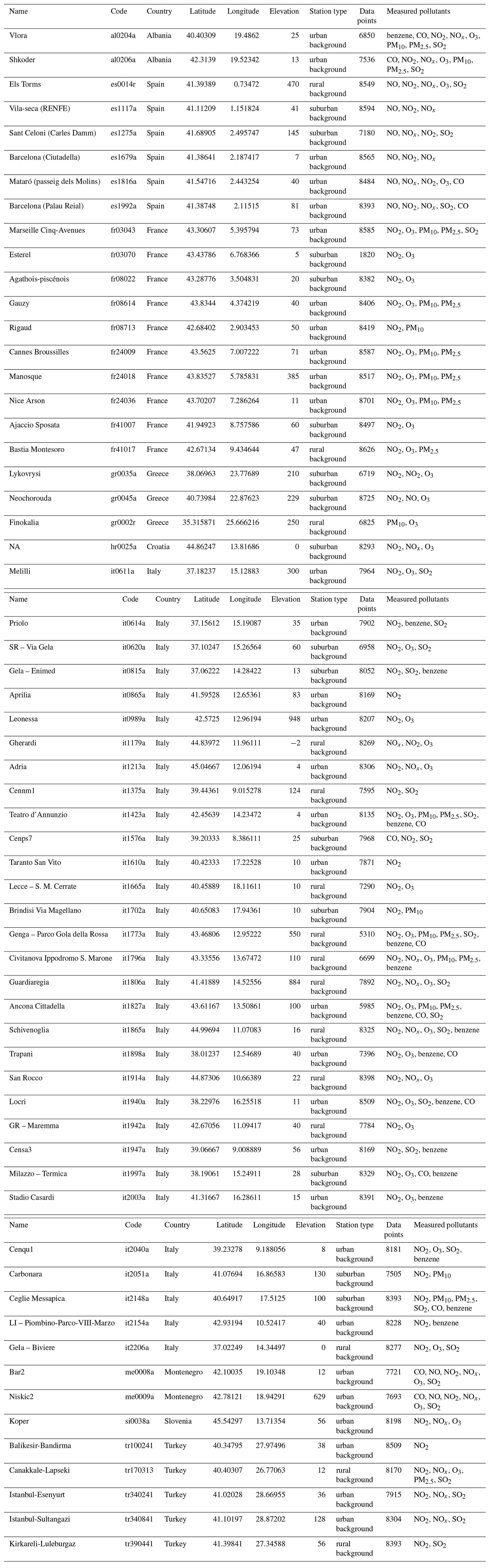
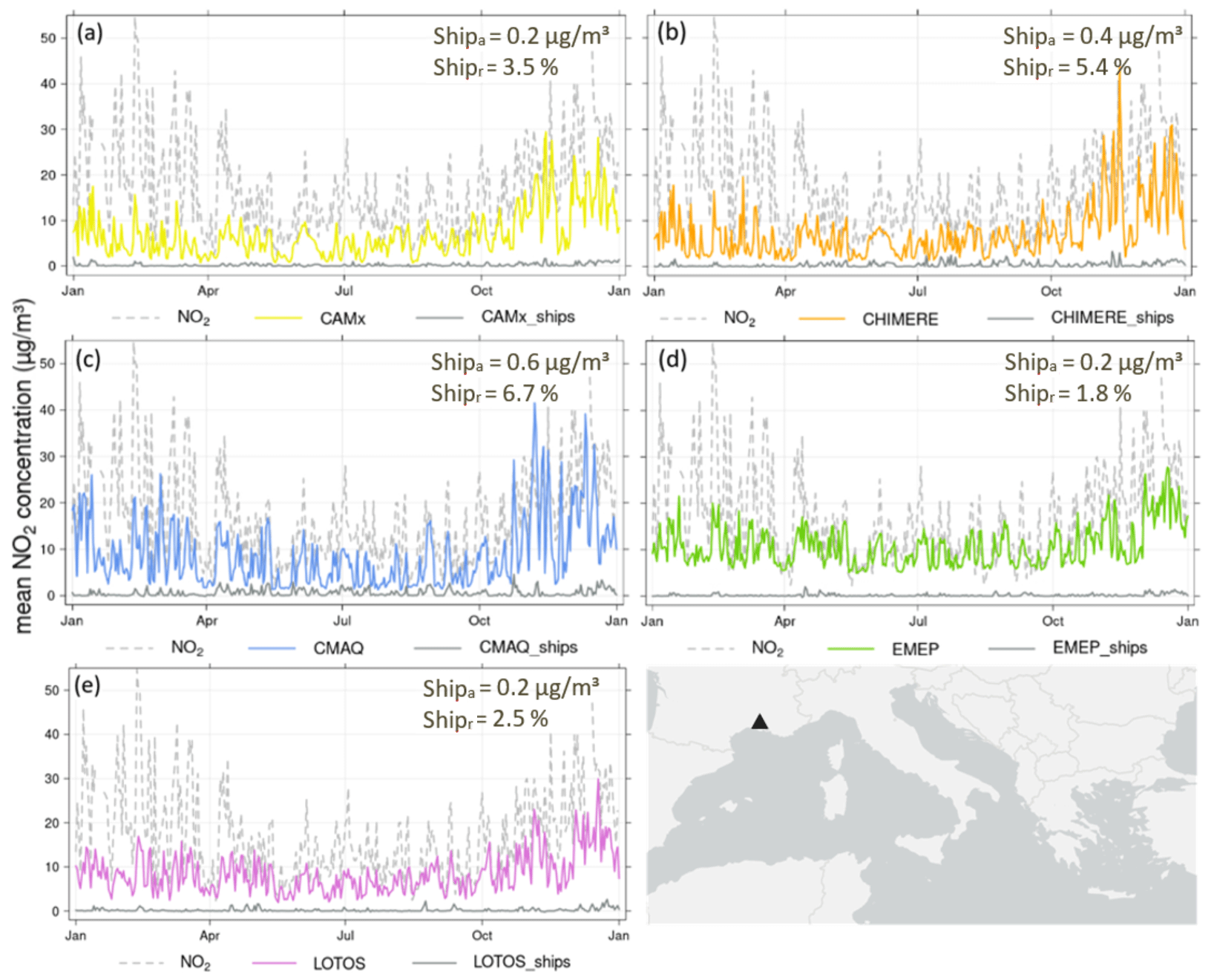
Figure C1Time series with daily mean NO2 concentrations in 2015 at station fr08614 in France. The black triangle on the map (bottom right) displays the location of the station. (a) CAMx; (b) CHIMERE; (c) CMAQ; (d) EMEP; (e) LOTOS-EUROS. Dashed gray line – measured data; colored lines – modeled data; gray line – modeled potential ship impact. Correlation between modeled and measured data for hourly total emission data for 2015: CAMx =0.23; CHIMERE =0.20; CMAQ =0.60; EMEP =0.02; LOTOS-EUROS =0.65. Shipa: potential absolute ship impact; Shipr: potential relative ship impact of the respective model.
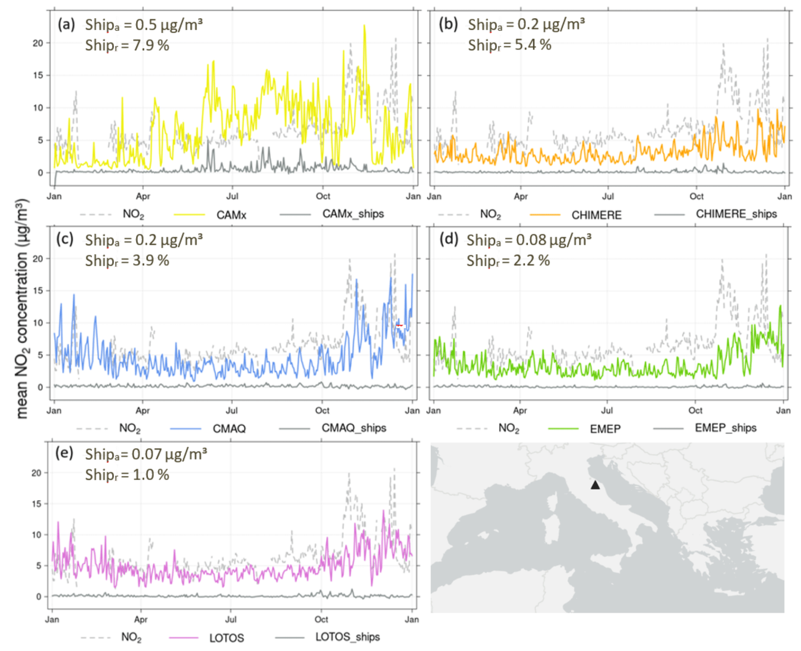
Figure C2Time series with daily mean NO2 concentration in 2015 at station it1773a in Italy. The black triangle on the map (bottom right) displays the location of the station. (a) CAMx; (b) CHIMERE; (c) CMAQ; (d) EMEP; (e) LOTOS-EUROS. Dashed gray line – measured data; colored lines – modeled data; gray line – modeled potential ship impact. Correlation between modeled and measured data for hourly total emission data for 2015: CAMx =0.03; CHIMERE =0.03; CMAQ =0.20; EMEP ; LOTOS-EUROS =0.14 Shipa: potential absolute ship impact; Shipr: potential relative ship impact of the respective model.

Figure C3Time series with daily mean NO2 concentration in 2015 at station gr0035a in Greece. The black triangle on the map (bottom right) displays the location of the station. (a) CAMx; (b) CHIMERE; (c) CMAQ; (d) EMEP; (e) LOTOS-EUROS. Dashed gray line – measured data; colored lines – modeled data; gray line – modeled potential ship impact. Correlation between modeled and measured data for hourly total emission data for 2015: CAMx =0.15; CHIMERE =0.20; CMAQ =0.28; EMEP =0.55; LOTOS-EUROS =0.38. Shipa: potential absolute ship impact; Shipr: potential relative ship impact of the respective model.
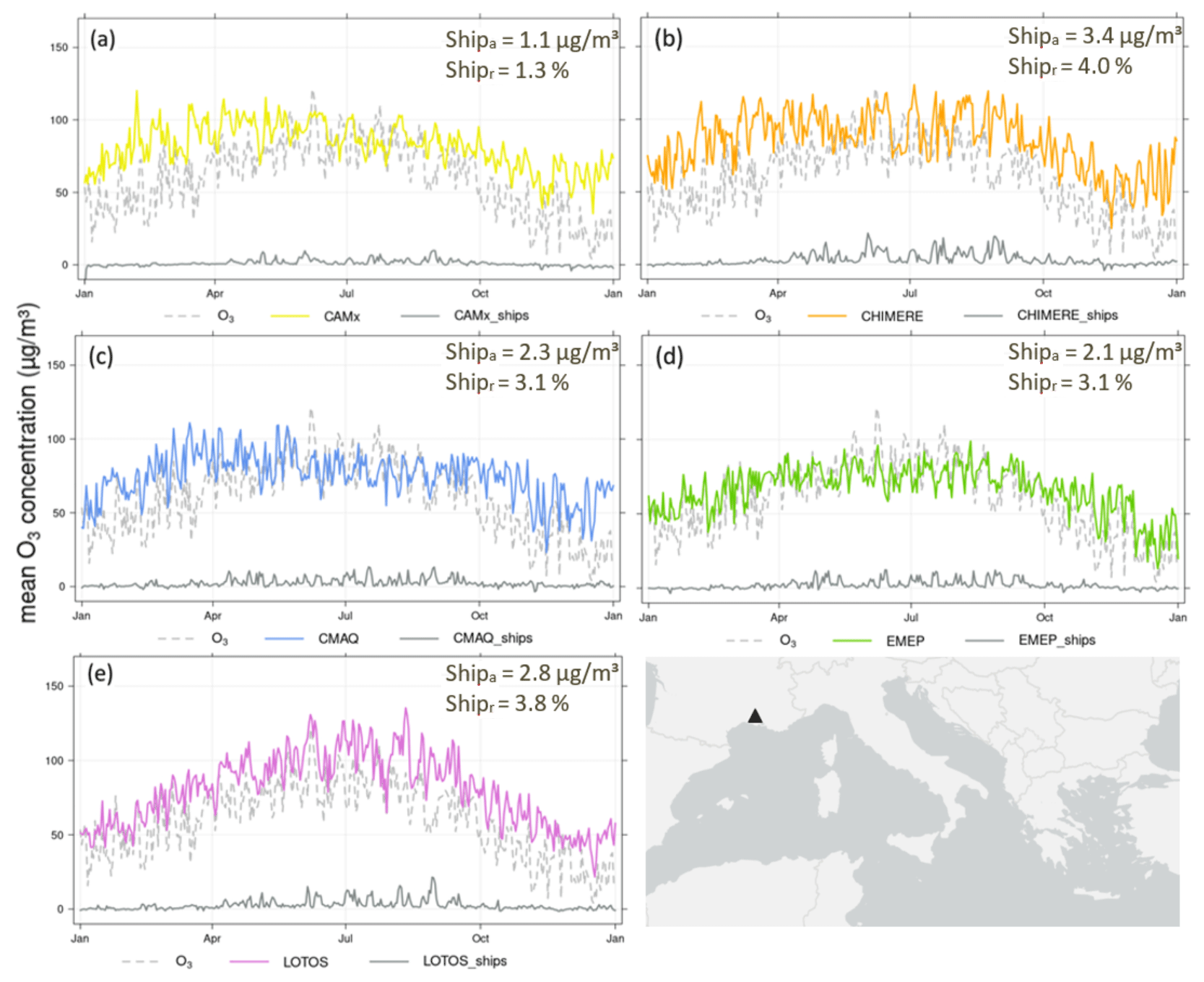
Figure D1Time series with daily mean O3 concentration in 2015 at station fr08614 in France. The black triangle on the map (bottom right) displays the location of the station. (a) CAMx; (b) CHIMERE; (c) CMAQ; (d) EMEP; (e) LOTOS-EUROS. Dashed gray line – measured data; colored lines – modeled data; gray line – modeled potential ship impact. Correlation between modeled and measured data for hourly total emission data for 2015: CAMx =0.57; CHIMERE =0.6; CMAQ =0.71; EMEP =0.39; LOTOS-EUROS =0.78. Shipa: potential absolute ship impact; Shipr: potential relative ship impact of the respective model.

Figure D2Time series with daily mean O3 concentration in 2015 at station it1773a in Italy. The black triangle on the map (bottom right) displays the location of the station. (a) CAMx; (b) CHIMERE; (c) CMAQ; (d) EMEP; (e) LOTOS-EUROS. Dashed gray line – measured data; colored lines – modeled data; gray line – modeled potential ship impact. Correlation between modeled and measured data for hourly total emission data for 2015: CAMx =0.37; CHIMERE =0.4; CMAQ =0.58; EMEP =0.35; LOTOS-EUROS =0.7. Shipa: potential absolute ship impact; Shipr: potential relative ship impact of the respective model.
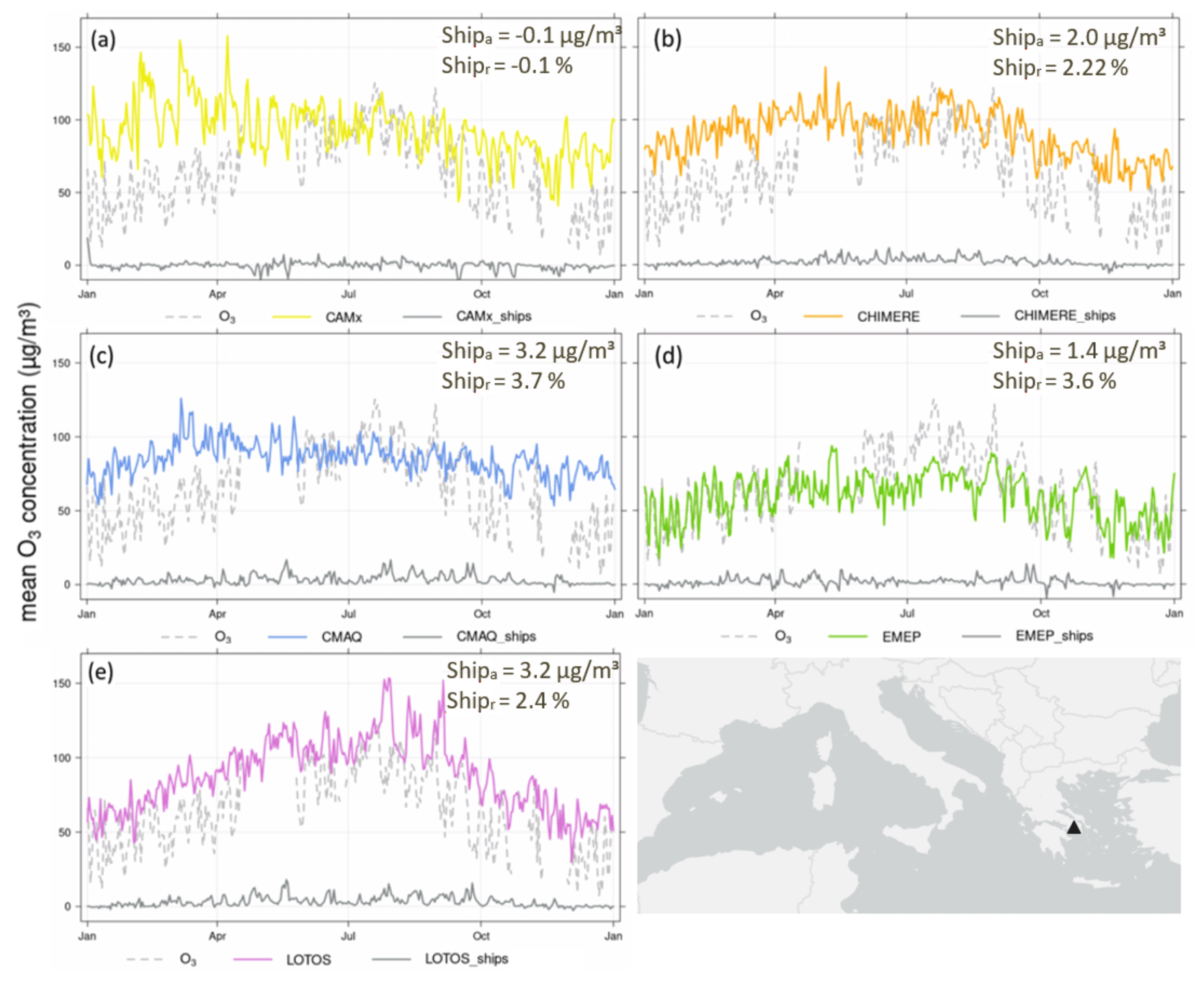
Figure D3Time series with daily mean O3 concentration in 2015 at station gr0035a in Greece. The black triangle on the map (bottom right) displays the location of the station. (a) CAMx; (b) CHIMERE; (c) CMAQ; (d) EMEP; (e) LOTOS-EUROS. Dashed gray line – measured data; colored lines – modeled data; gray line – modeled potential ship impact. Correlation between modeled and measured data for hourly total emission data for 2015: CAMx =0.29; CHIMERE =0.46; CMAQ =0.50; EMEP =0.71; LOTOS-EUROS =0.57. Shipa: potential absolute ship impact; Shipr: potential relative ship impact of the respective model.

Figure E1Annual mean of NOx total concentration. (a) CAMx; (b) CHIMERE; (c) CMAQ; (d) LOTOS-EUROS. Below the domain figure the respective frequency distribution is displayed for the annual mean NOx concentration, referring to the whole model domain.

Figure E2Annual mean relative potential ship impact of NOx. (a) CAMx; (b) CHIMERE; (c) CMAQ; (d) LOTOS-EUROS. Below the domain figure the respective frequency distribution is displayed for the annual mean relative potential ship impact of NOx, referring to the whole model domain.
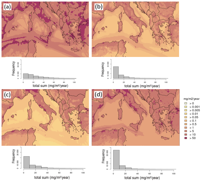
Figure F1Annual total dry deposition of N. (a) CAMx; (b) CHIMERE; (c) CMAQ; (d) LOTOS-EUROS.
CAMx source code and documentation can be downloaded from https://camx-wp.azurewebsites.net/download/source/ (last access: 19 January 2023; Ramboll, 2023) and the Chimere website (https://www.lmd.polytechnique.fr/chimere/2020_getcode.php, last access: 19 January 2023). CMAQ version 5.2, which was used here, is available at https://doi.org/10.5281/zenodo.1167892 (US EPA Office of Research and Development, 2017). EMEP is available at https://doi.org/10.5281/zenodo.3647990 (EMEP MSC-W, 2020), LOTOS-EUROS is available at https://lotos-euros.tno.nl/open-source-version/ (last access: 19 January 2023; TNO, 2023), and WPS/WRF is available from WPS (2022; https://github.com/wrf-model/WPS, last access: 19 January 2023) and WRF Community (2000, https://doi.org/10.5065/D6MK6B4K). The COSMO software is available at https://www.cosmo-model.org/content/support/software/default.htm#models (last access: 24 January 2023; COSMO, 2023) and ecmwf-ifs/ifs-scripts at https://github.com/ecmwf-ifs (last access: 19 January 2023; ECMWF, 2023).
Data on measurement stations from EEA can be downloaded at https://discomap.eea.europa.eu/map/fme/AirQualityExport.htm (last access: 20 January 2023). CTM model results are available upon request.
The supplement related to this article is available online at: https://doi.org/10.5194/acp-23-1825-2023-supplement.
LF: CMAQ model runs, evaluation and analysis of model results, preparation and writing of the paper. MK: Analysis of the results, revision of the text. VM: Supervision, analysis of the results, revision of the text. SO: CAMx and CHIMERE model runs, discussion of the results. RK and JK: LOTOS-EUROS model runs, land-based emissions data provision, discussion of the results. JM and SJ: EMEP model runs, discussion of the results. JPJ and EM: STEAM model runs, shipping emissions data provision, discussion of the results.
The contact author has declared that none of the authors has any competing interests.
Publisher’s note: Copernicus Publications remains neutral with regard to jurisdictional claims in published maps and institutional affiliations.
This was work supported by the SCIPPER project, which has received funding from the European Union's Horizon 2020 research and innovation program under grant agreement no. 814893.
The Community Multiscale Air Quality Modeling System (CMAQ) is developed and maintained by the USEPA. Its use is gratefully acknowledged. Ronny Petrik from Helmholtz Centre Hereon is acknowledged for providing meteorology and boundary conditions for CMAQ runs.
The computations for the regional modeling using the EMEP model was enabled by resources provided by the Swedish National Infrastructure for Computing (SNIC), partially funded by the Swedish Research Council through grant agreement no. 2018-05973.
Support from the Meteorological Synthesizing Center–West of EMEP at the Norwegian Meteorological Institute, especially from Peter Wind and David Simpson, for the implementation of emissions and meteorological fields used in this paper in the EMEP open-source model is gratefully acknowledged.
This research has been supported by the European Union's Horizon 2020 (SCIPPER (grant no. 814893)) and the Swedish Research Council (grant agreement no. 2018-05973).
The article processing charges for this open-access publication were covered by the Helmholtz-Zentrum Hereon.
This paper was edited by Andrea Pozzer and reviewed by two anonymous referees.
Agrawal, H., Welch, W. A., Miller, J. W., and Cockert, D. R.: Emission measurements from a crude oil tanker at sea, Environ. Sci. Technol., 42, 7098–7103, https://doi.org/10.1021/es703102y, 2008.
Agrawal, H., Welch, W. A., Henningsen, S., Miller, J. W., and Cocker, D. R.: Emissions from main propulsion engine on container ship at sea, J. Geophys. Res., 115, D23205, https://doi.org/10.1029/2009JD013346, 2010.
Aksoyoglu, S., Baltensperger, U., and Prévôt, A. S. H.: Contribution of ship emissions to the concentration and deposition of air pollutants in Europe, Atmos. Chem. Phys., 16, 1895–1906, https://doi.org/10.5194/acp-16-1895-2016, 2016.
Anav, A., Proietti, C., Menut, L., Carnicelli, S., De Marco, A., and Paoletti, E.: Sensitivity of stomatal conductance to soil moisture: implications for tropospheric ozone, Atmos. Chem. Phys., 18, 5747–5763, https://doi.org/10.5194/acp-18-5747-2018, 2018.
Appel, K. W., Napelenok, S. L., Foley, K. M., Pye, H. O. T., Hogrefe, C., Luecken, D. J., Bash, J. O., Roselle, S. J., Pleim, J. E., Foroutan, H., Hutzell, W. T., Pouliot, G. A., Sarwar, G., Fahey, K. M., Gantt, B., Gilliam, R. C., Heath, N. K., Kang, D., Mathur, R., Schwede, D. B., Spero, T. L., Wong, D. C., and Young, J. O.: Description and evaluation of the Community Multiscale Air Quality (CMAQ) modeling system version 5.1, Geosci. Model Dev., 10, 1703–1732, https://doi.org/10.5194/gmd-10-1703-2017, 2017.
Astitha, M., Lelieveld, J., Abdel Kader, M., Pozzer, A., and de Meij, A.: Parameterization of dust emissions in the global atmospheric chemistry-climate model EMAC: impact of nudging and soil properties, Atmos. Chem. Phys., 12, 11057–11083, https://doi.org/10.5194/acp-12-11057-2012, 2012.
Aulinger, A., Matthias, V., Zeretzke, M., Bieser, J., Quante, M., and Backes, A.: The impact of shipping emissions on air pollution in the greater North Sea region – Part 1: Current emissions and concentrations, Atmos. Chem. Phys., 16, 739–758, https://doi.org/10.5194/acp-16-739-2016, 2016.
Baldasano, J. M., Pay, M. T., Jorba, O., Gassó, S., and Jiménez-Guerrero, P.: An annual assessment of air quality with the CALIOPE modeling system over Spain, Sci. Total Environ., 409, 2163–2178, https://doi.org/10.1016/j.scitotenv.2011.01.041, 2011.
Barregard, L., Molnàr, P., Jonson, J. E., and Stockfelt, L.: Impact on Population Health of Baltic Shipping Emissions, Int. J. Environ. Res. Pu., 16, 1954, https://doi.org/10.3390/ijerph16111954, 2019.
Beltman, J. B., Hendriks, C., Tum, M., and Schaap, M.: The impact of large scale biomass production on ozone air pollution in Europe, Atmos. Environ., 71, 352–363, https://doi.org/10.1016/j.atmosenv.2013.02.019, 2013.
Bergström, R., Denier van der Gon, H. A. C., Prévôt, A. S. H., Yttri, K. E., and Simpson, D.: Modelling of organic aerosols over Europe (2002–2007) using a volatility basis set (VBS) framework: application of different assumptions regarding the formation of secondary organic aerosol, Atmos. Chem. Phys., 12, 8499–8527, https://doi.org/10.5194/acp-12-8499-2012, 2012.
Bessagnet, B., Pirovano, G., Mircea, M., Cuvelier, C., Aulinger, A., Calori, G., Ciarelli, G., Manders, A., Stern, R., Tsyro, S., García Vivanco, M., Thunis, P., Pay, M.-T., Colette, A., Couvidat, F., Meleux, F., Rouïl, L., Ung, A., Aksoyoglu, S., Baldasano, J. M., Bieser, J., Briganti, G., Cappelletti, A., D'Isidoro, M., Finardi, S., Kranenburg, R., Silibello, C., Carnevale, C., Aas, W., Dupont, J.-C., Fagerli, H., Gonzalez, L., Menut, L., Prévôt, A. S. H., Roberts, P., and White, L.: Presentation of the EURODELTA III intercomparison exercise – evaluation of the chemistry transport models' performance on criteria pollutants and joint analysis with meteorology, Atmos. Chem. Phys., 16, 12667–12701, https://doi.org/10.5194/acp-16-12667-2016, 2016.
Bieser, J., Aulinger, A., Matthias, V., Quante, M., and Builtjes, P.: SMOKE for Europe – adaptation, modification and evaluation of a comprehensive emission model for Europe, Geosci. Model Dev., 4, 47–68, https://doi.org/10.5194/gmd-4-47-2011, 2011a.
Bieser, J., Aulinger, A., Matthias, V., Quante, M., and Denier van der Gon, H. A. C.: Vertical emission profiles for Europe based on plume rise calculations, Environ. Pollut., 159, 2935–2946, https://doi.org/10.1016/j.envpol.2011.04.030, 2011b.
Binkowski, F. S. and Shankar, U.: The Regional Particulate Matter Model: 1. Model description and preliminary results, J. Geophys. Res., 100, 26191–26209, https://doi.org/10.1029/95JD02093, 1995.
Bobbink, R. and Hettelingh, J.-P. (Eds.): Review and revision of empirical critical loads and dose-response relationships, RIVM report: 680359002, 246 pp., https://www.rivm.nl/bibliotheek/rapporten/680359002.pdf (last access: 20 January 2023), 2011.
Brandt, J., Silver, J. D., Christensen, J. H., Andersen, M. S., Bønløkke, J. H., Sigsgaard, T., Geels, C., Gross, A., Hansen, A. B., Hansen, K. M., Hedegaard, G. B., Kaas, E., and Frohn, L. M.: Contribution from the ten major emission sectors in Europe and Denmark to the health-cost externalities of air pollution using the EVA model system – an integrated modelling approach, Atmos. Chem. Phys., 13, 7725–7746, https://doi.org/10.5194/acp-13-7725-2013, 2013.
Byun, D. and Schere, K. L.: Review of the Governing Equations, Computational Algorithms, and Other Components of the Models-3 Community Multiscale Air Quality (CMAQ) Modeling System, Appl. Mech. Rev., 2, 51–77, https://doi.org/10.1115/1.2128636, 2006.
Carlton, A. G., Bhave, P. V., Napelenok, S. L., Edney, E. O., Sarwar, G., Pinder, R. W., Pouliot, G. A., and Houyoux, M.: Model representation of secondary organic aerosol in CMAQv4.7, Environ. Sci. Technol., 44, 8553–8560, https://doi.org/10.1021/es100636q, 2010.
Celik, S., Drewnick, F., Fachinger, F., Brooks, J., Darbyshire, E., Coe, H., Paris, J.-D., Eger, P. G., Schuladen, J., Tadic, I., Friedrich, N., Dienhart, D., Hottmann, B., Fischer, H., Crowley, J. N., Harder, H., and Borrmann, S.: Influence of vessel characteristics and atmospheric processes on the gas and particle phase of ship emission plumes: in situ measurements in the Mediterranean Sea and around the Arabian Peninsula, Atmos. Chem. Phys., 20, 4713–4734, https://doi.org/10.5194/acp-20-4713-2020, 2020.
Chimere: Download source code and databases, https://www.lmd.polytechnique.fr/chimere/2020_getcode.php, last access: 19 January 2023.
Clapp, L. J. and Jenkin, M. E.: Analysis of the relationship between ambient levels of O3, NO2 and NO as a function of NOx in the UK, Atmos. Environ., 35, 6391–6405, https://doi.org/10.1016/S1352-2310(01)00378-8, 2001.
Clifton, O. E., Fiore, A. M., Massman, W. J., Baublitz, C. B., Coyle, M., Emberson, L., Fares, S., Farmer, D. K., Gentine, P., Gerosa, G., Guenther, A. B., Helmig, D., Lombardozzi, D. L., Munger, J. W., Patton, E. G., Pusede, S. E., Schwede, D. B., Silva, S. J., Sörgel, M., Steiner, A. L., and Tai, A. P. K.: Dry Deposition of Ozone over Land: Processes, Measurement, and Modeling, Rev. Geophys., 58, e2019RG000670, https://doi.org/10.1029/2019RG000670, 2020.
Cofala., J., Amann, M., Borken-Kleefeld, J., Gomez-Sanabria, A., Heyes, C., Kiesewetter, G., Sander, R., Schoepp, W., Holland, M., Fagerli, H., and Nyiri, A.: The potential for cost-effective air emission reductions from international shipping through designation of further Emission Control Areas in EU waters with focus on the Mediterranean Sea, Final Report, IIASA, Austria, https://previous.iiasa.ac.at/web/home/research/researchPrograms/air/Shipping_emissions_reductions_main.pdf (last access: 20 January 2023), 2018.
Colette, A., Andersson, C., Manders, A., Mar, K., Mircea, M., Pay, M.-T., Raffort, V., Tsyro, S., Cuvelier, C., Adani, M., Bessagnet, B., Bergström, R., Briganti, G., Butler, T., Cappelletti, A., Couvidat, F., D'Isidoro, M., Doumbia, T., Fagerli, H., Granier, C., Heyes, C., Klimont, Z., Ojha, N., Otero, N., Schaap, M., Sindelarova, K., Stegehuis, A. I., Roustan, Y., Vautard, R., van Meijgaard, E., Vivanco, M. G., and Wind, P.: EURODELTA-Trends, a multi-model experiment of air quality hindcast in Europe over 1990–2010, Geosci. Model Dev., 10, 3255–3276, https://doi.org/10.5194/gmd-10-3255-2017, 2017.
Contini, D. and Merico, E.: Recent Advances in Studying Air Quality and Health Effects of Shipping Emissions, Atmosphere, 12, 92, https://doi.org/10.3390/atmos12010092, 2021.
Corbett, J. J. and Fischbeck, P.: Emissions from ships, Science, 278, 823–824, 1997.
Corbett, J. J., Fischbeck, P., and Pandis, S.: Global nitrogen and sulfur inventories for oceangoing ships, J. Geophys. Res.-Atmos., 104, 3457–3470, 1999.
COSMO: COSMO software, COSMO [code], https://www.cosmo-model.org/content/support/software/default.htm#models, last access: 24 January 2023.
Doche, C., Dufour, G., Foret, G., Eremenko, M., Cuesta, J., Beekmann, M., and Kalabokas, P.: Summertime tropospheric-ozone variability over the Mediterranean basin observed with IASI, Atmos. Chem. Phys., 14, 10589–10600, https://doi.org/10.5194/acp-14-10589-2014, 2014.
Donahue, N. M., Robinson, A. L., and Pandis, S. N.: Atmospheric organic particulate matter: From smoke to secondary organic aerosol, Atmos. Environ, 43, 94–106, https://doi.org/10.1016/j.atmosenv.2008.09.055, 2009.
Donateo, A., Gregoris, E., Gambaro, A., Merico, E., Giua, R., Nocioni, A., and Contini, D.: Contribution of harbour activities and ship traffic to PM2.5, particle number concentrations and PAHs in a port city of the Mediterranean Sea (Italy), Environ. Sci. Pollut. Res., 21, 9415–9429, https://doi.org/10.1007/s11356-014-2849-0, 2014.
ECMWF: ecmwf-ifs/ifs-scripts, GitHub, https://github.com/ecmwf-ifs, last access: 19 January 2023.
EEA: Download of air quality data, EEA [data set], https://discomap.eea.europa.eu/map/fme/AirQualityExport.htm, last access: 20 January 2023.
Emberson, L. D., Simpson, D., Tuovinen, J.-P., Ashmore, M. R., and Cambridge, H. M.: Towards a Model of Ozone Deposition and Stomatal Uptake over Europe, Norwegian Meteorological Institute, Oslo, EMEP/MSC-W Note 6/00, 57 pp., 2000.
EMEP MSC-W: metno/emep-ctm: OpenSource rv4.34 (202001), Version rv4_34, Zenodo [software], https://doi.org/10.5281/zenodo.3647990, 2020.
Emerson, E. W., Hodshire, A. L., DeBolt, H. M., Bilsback, K. R., Pierce, J. R., McMeeking, G. R., and Farmer, D. K.: Revisiting particle dry deposition and its role in radiative effect estimates, P. Natl. Acad. Sci. USA, 117, 26076–26082, https://doi.org/10.1073/pnas.2014761117, 2020.
Endresen, Ø., Sørgård, E., Sundet, J. K., Dalsøren, S. B., Isaksen, I. S., Berglen, T. F., and Gravir, G.: Emission from international sea transportation and environmental impact, J. Geophys. Res., 108, 4560, https://doi.org/10.1029/2002JD002898, 2003.
EPA: Health Effects of Ozone Pollution, https://www.epa.gov/ground-level-ozone-pollution/health-effects-ozone-pollution (last access: 23 March 2022), 2021.
Erisman, J. W., van Pul, A., and Wyers, P.: Parametrization of surface resistance for the quantification of atmospheric deposition of acidifying pollutants and ozone, Atmos. Environ., 28, 2595–2607, https://doi.org/10.1016/1352-2310(94)90433-2, 1994.
Eurostat Press Office: World Maritime Day. Half of EU trade in goods is carried by sea, Eurostat Press Office, News Release 184/2016, https://ec.europa.eu/eurostat/documents/2995521/7667714/6-28092016-AP-EN.pdf (last access: 20 January 2023), 2016.
Eyring, V., Isaksen, I. S.A., Berntsen, T., Collins, W. J., Corbett, J. J., Endresen, O., Grainger, R. G., Moldanova, J., Schlager, H., and Stevenson, D. S.: Transport impacts on atmosphere and climate: Shipping, Atmos. Environ., 44, 4735–4771, https://doi.org/10.1016/j.atmosenv.2009.04.059, 2010.
Fountoukis, C. and Nenes, A.: ISORROPIA II: a computationally efficient thermodynamic equilibrium model for K+–Ca2+–Mg2+–NH4+–Na+–SO–NO–Cl−–H2O aerosols, Atmos. Chem. Phys., 7, 4639–4659, https://doi.org/10.5194/acp-7-4639-2007, 2007.
Friedrich, N., Eger, P., Shenolikar, J., Sobanski, N., Schuladen, J., Dienhart, D., Hottmann, B., Tadic, I., Fischer, H., Martinez, M., Rohloff, R., Tauer, S., Harder, H., Pfannerstill, E. Y., Wang, N., Williams, J., Brooks, J., Drewnick, F., Su, H., Li, G., Cheng, Y., Lelieveld, J., and Crowley, J. N.: Reactive nitrogen around the Arabian Peninsula and in the Mediterranean Sea during the 2017 AQABA ship campaign, Atmos. Chem. Phys., 21, 7473–7498, https://doi.org/10.5194/acp-21-7473-2021, 2021.
Galmarini, S., Makar, P., Clifton, O. E., Hogrefe, C., Bash, J. O., Bellasio, R., Bianconi, R., Bieser, J., Butler, T., Ducker, J., Flemming, J., Hodzic, A., Holmes, C. D., Kioutsioukis, I., Kranenburg, R., Lupascu, A., Perez-Camanyo, J. L., Pleim, J., Ryu, Y.-H., San Jose, R., Schwede, D., Silva, S., and Wolke, R.: Technical note: AQMEII4 Activity 1: evaluation of wet and dry deposition schemes as an integral part of regional-scale air quality models, Atmos. Chem. Phys., 21, 15663–15697, https://doi.org/10.5194/acp-21-15663-2021, 2021.
Ginoux, P., Chin, M., Tegen, I., Prospero, J. M., Holben, B., Dubovik, O., and Lin, S.-J.: Sources and distributions of dust aerosols simulated with the GOCART model, J. Geophys. Res., 106, 20255–20273, https://doi.org/10.1029/2000JD000053, 2001.
Giordano, L., Brunner, D., Flemming, J., Hogrefe, C., Im, U., Bianconi, R., Badia, A., Balzarini, A., Baró, R., Chemel, C., Curci, G., Forkel, R., Jiménez-Guerrero, P., Hirtl, M., Hodzic, A., Honzak, L., Jorba, O., Knote, C., Kuenen, J.J.P., Makar, P. A., Manders-Groot, A., Neal, L., Pérez, J. L., Pirovano, G., Pouliot, G., San José, R., Savage, N., Schröder, W., Sokhi, R. S., Syrakov, D., Torian, A., Tuccella, P., Werhahn, J., Wolke, R., Yahya, K., Žabkar, R., Zhang, Y., and Galmarini, S.: Assessment of the MACC reanalysis and its influence as chemical boundary conditions for regional air quality modeling in AQMEII-2, Atmos. Environ., 115, 371–388, https://doi.org/10.1016/j.atmosenv.2015.02.034, 2015.
Gong, S. L.: A parameterization of sea-salt aerosol source function for sub- and super-micron particles, Global Biogeochem. Cy., 17, 1097, https://doi.org/10.1029/2003gb002079, 2003.
Granier, C., Darras, S., van der Denier Gon, H., Doubalova, J., Elguindi, N., Galle, B., Gauss, M., Guevara, M., Jalkanen, J.-P., Kuenen, J., Liousse, C., Quack, B., Simpson, D., and Sindelarova, K.: The Copernicus Atmosphere Monitoring Service global and regional emissions: (April 2019 version), Copernicus Atmosphere Monitoring Service (CAMS) report, https://doi.org/10.24380/d0bn-kx16, 2019.
Guenther, A., Karl, T., Harley, P., Wiedinmyer, C., Palmer, P. I., and Geron, C.: Estimates of global terrestrial isoprene emissions using MEGAN (Model of Emissions of Gases and Aerosols from Nature), Atmos. Chem. Phys., 6, 3181–3210, https://doi.org/10.5194/acp-6-3181-2006, 2006.
Guenther, A. B., Jiang, X., Heald, C. L., Sakulyanontvittaya, T., Duhl, T., Emmons, L. K., and Wang, X.: The Model of Emissions of Gases and Aerosols from Nature version 2.1 (MEGAN2.1): an extended and updated framework for modeling biogenic emissions, Geosci. Model Dev., 5, 1471–1492, https://doi.org/10.5194/gmd-5-1471-2012, 2012.
Hardacre, C., Wild, O., and Emberson, L.: An evaluation of ozone dry deposition in global scale chemistry climate models, Atmos. Chem. Phys., 15, 6419–6436, https://doi.org/10.5194/acp-15-6419-2015, 2015.
Hicks, B. B., Baldocchi, D. D., Meyers, T. P., Hosker, R. P., and Matt, D. R.: A preliminary multiple resistance routine for deriving dry deposition velocities from measured quantities, Water Air Soil Pollut., 36, 311–330, https://doi.org/10.1007/BF00229675, 1987.
Im, U., Christodoulaki, S., Violaki, K., Zarmpas, P., Kocak, M., Daskalakis, N., Mihalopoulos, N., and Kanakidou, M.: Atmospheric deposition of nitrogen and sulfur over southern Europe with focus on the Mediterranean and the Black Sea, Atmos. Environ., 81, 660–670, https://doi.org/10.1016/j.atmosenv.2013.09.048, 2013.
Im, U., Bianconi, R., Solazzo, E., Kioutsioukis, I., Badia, A., Balzarini, A., Baró, R., Bellasio, R., Brunner, D., Chemel, C., Curci, G., Flemming, J., Forkel, R., Giordano, L., Jiménez-Guerrero, P., Hirtl, M., Hodzic, A., Honzak, L., Jorba, O., Knote, C., Kuenen, J. J.P., Makar, P. A., Manders-Groot, A., Neal, L., Pérez, J. L., Pirovano, G., Pouliot, G., San Jose, R., Savage, N., Schroder, W., Sokhi, R. S., Syrakov, D., Torian, A., Tuccella, P., Werhahn, J., Wolke, R., Yahya, K., Zabkar, R., Zhang, Y., Zhang, J., Hogrefe, C., and Galmarini, S.: Evaluation of operational on-line-coupled regional air quality models over Europe and North America in the context of AQMEII phase 2. Part I: Ozone, Atmos. Environ., 115, 404–420, https://doi.org/10.1016/j.atmosenv.2014.09.042, 2015a.
Im, U., Bianconi, R., Solazzo, E., Kioutsioukis, I., Badia, A., Balzarini, A., Baró, R., Bellasio, R., Brunner, D., Chemel, C., Curci, G., van der Denier Gon, H., Flemming, J., Forkel, R., Giordano, L., Jiménez-Guerrero, P., Hirtl, M., Hodzic, A., Honzak, L., Jorba, O., Knote, C., Makar, P. A., Manders-Groot, A., Neal, L., Pérez, J. L., Pirovano, G., Pouliot, G., San Jose, R., Savage, N., Schroder, W., Sokhi, R. S., Syrakov, D., Torian, A., Tuccella, P., Wang, K., Werhahn, J., Wolke, R., Zabkar, R., Zhang, Y., Zhang, J., Hogrefe, C., and Galmarini, S.: Evaluation of operational online-coupled regional air quality models over Europe and North America in the context of AQMEII phase 2. Part II: Particulate matter, Atmos. Environ., 115, 421–441, https://doi.org/10.1016/j.atmosenv.2014.08.072, 2015b.
Inness, A., Ades, M., Agustí-Panareda, A., Barré, J., Benedictow, A., Blechschmidt, A.-M., Dominguez, J. J., Engelen, R., Eskes, H., Flemming, J., Huijnen, V., Jones, L., Kipling, Z., Massart, S., Parrington, M., Peuch, V.-H., Razinger, M., Remy, S., Schulz, M., and Suttie, M.: The CAMS reanalysis of atmospheric composition, Atmos. Chem. Phys., 19, 3515–3556, https://doi.org/10.5194/acp-19-3515-2019, 2019.
Jägerbrand, A. K., Brutemark, A., Barthel Svedén, J., and Gren, I.-M.: A review on the environmental impacts of shipping on aquatic and nearshore ecosystems, Sci. Total Environ., 695, 133637, https://doi.org/10.1016/j.scitotenv.2019.133637, 2019.
Jalkanen, J.-P., Brink, A., Kalli, J., Pettersson, H., Kukkonen, J., and Stipa, T.: A modelling system for the exhaust emissions of marine traffic and its application in the Baltic Sea area, Atmos. Chem. Phys., 9, 9209–9223, https://doi.org/10.5194/acp-9-9209-2009, 2009.
Jalkanen, J.-P., Johansson, L., Kukkonen, J., Brink, A., Kalli, J., and Stipa, T.: Extension of an assessment model of ship traffic exhaust emissions for particulate matter and carbon monoxide, Atmos. Chem. Phys., 12, 2641–2659, https://doi.org/10.5194/acp-12-2641-2012, 2012.
Jalkanen, J.-P., Johansson, L., and Kukkonen, J.: A comprehensive inventory of ship traffic exhaust emissions in the European sea areas in 2011, Atmos. Chem. Phys., 16, 71–84, https://doi.org/10.5194/acp-16-71-2016, 2016.
Johansson, L., Jalkanen, J.-P., Kalli, J., and Kukkonen, J.: The evolution of shipping emissions and the costs of regulation changes in the northern EU area, Atmos. Chem. Phys., 13, 11375–11389, https://doi.org/10.5194/acp-13-11375-2013, 2013.
Johansson, L., Jalkanen, J.-P., and Kukkonen, J.: Global assessment of shipping emissions in 2015 on a high spatial and temporal resolution, Atmos. Environ., 167, 403–415, https://doi.org/10.1016/j.atmosenv.2017.08.042, 2017.
Jonson, J. E., Jalkanen, J. P., Johansson, L., Gauss, M., and Denier van der Gon, H. A. C.: Model calculations of the effects of present and future emissions of air pollutants from shipping in the Baltic Sea and the North Sea, Atmos. Chem. Phys., 15, 783–798, https://doi.org/10.5194/acp-15-783-2015, 2015.
Jutterström, S., Moldan, F., Moldanová, J., Karl, M., Matthias, V., and Posch, M.: The impact of nitrogen and sulfur emissions from shipping on the exceedance of critical loads in the Baltic Sea region, Atmos. Chem. Phys., 21, 15827–15845, https://doi.org/10.5194/acp-21-15827-2021, 2021.
Karl, M., Bieser, J., Geyer, B., Matthias, V., Jalkanen, J.-P., Johansson, L., and Fridell, E.: Impact of a nitrogen emission control area (NECA) on the future air quality and nitrogen deposition to seawater in the Baltic Sea region, Atmos. Chem. Phys., 19, 1721–1752, https://doi.org/10.5194/acp-19-1721-2019, 2019a.
Karl, M., Jonson, J. E., Uppstu, A., Aulinger, A., Prank, M., Sofiev, M., Jalkanen, J.-P., Johansson, L., Quante, M., and Matthias, V.: Effects of ship emissions on air quality in the Baltic Sea region simulated with three different chemistry transport models, Atmos. Chem. Phys., 19, 7019–7053, https://doi.org/10.5194/acp-19-7019-2019, 2019b.
Kelly, J. T., Bhave, P. V., Nolte, C. G., Shankar, U., and Foley, K. M.: Simulating emission and chemical evolution of coarse sea-salt particles in the Community Multiscale Air Quality (CMAQ) model, Geosci. Model Dev., 3, 257–273, https://doi.org/10.5194/gmd-3-257-2010, 2010.
Klingmüller, K., Metzger, S., Abdelkader, M., Karydis, V. A., Stenchikov, G. L., Pozzer, A., and Lelieveld, J.: Revised mineral dust emissions in the atmospheric chemistry–climate model EMAC (MESSy 2.52 DU_Astitha1 KKDU2017 patch), Geosci. Model Dev., 11, 989–1008, https://doi.org/10.5194/gmd-11-989-2018, 2018.
Knote, C., Tuccella, P., Curci, G., Emmons, L., Orlando, J. J., Madronich, S., Baró, R., Jiménez-Guerrero, P., Luecken, D., Hogrefe, C., Forkel, R., Werhahn, J., Hirtl, M., Pérez, J. L., San José, R., Giordano, L., Brunner, D., Yahya, K., and Zhang, Y.: Influence of the choice of gas-phase mechanism on predictions of key gaseous pollutants during the AQMEII phase-2 intercomparison, Atmos. Environ., 115, 553–568, https://doi.org/10.1016/j.atmosenv.2014.11.066, 2015.
Köhler, I., Sausen, R., and Reinberger, R.: Contributions of aircraft emissions to the atmospheric NOx content, Atmos. Environ., 31, 1801–1818, https://doi.org/10.1016/S1352-2310(96)00331-7, 1997.
Liu, J. J., Jones, D. B. A., Worden, J. R., Noone, D., Parrington, M., and Kar, J.: Analysis of the summertime buildup of tropospheric ozone abundances over the Middle East and North Africa as observed by the Tropospheric Emission Spectrometer instrument, J. Geophys. Res., 114, D05304, https://doi.org/10.1029/2008JD010993, 2009.
Manders, A. M. M., Builtjes, P. J. H., Curier, L., Denier van der Gon, H. A. C., Hendriks, C., Jonkers, S., Kranenburg, R., Kuenen, J. J. P., Segers, A. J., Timmermans, R. M. A., Visschedijk, A. J. H., Wichink Kruit, R. J., van Pul, W. A. J., Sauter, F. J., van der Swaluw, E., Swart, D. P. J., Douros, J., Eskes, H., van Meijgaard, E., van Ulft, B., van Velthoven, P., Banzhaf, S., Mues, A. C., Stern, R., Fu, G., Lu, S., Heemink, A., van Velzen, N., and Schaap, M.: Curriculum vitae of the LOTOS–EUROS (v2.0) chemistry transport model, Geosci. Model Dev., 10, 4145–4173, https://doi.org/10.5194/gmd-10-4145-2017, 2017.
Manders-Groot, A., Segers, A., and Jonkers, S.: LOTOS-EUROS v2.0 Reference Guide, TNO Report, TNO 2016 R10898, 77 pp., https://lotos-euros.tno.nl/media/10360/reference_guide_v2-0_r10898.pdf (last access: 20 January 2023), 2016.
Marmer, E. and Langmann, B.: Impact of ship emissions on the Mediterranean summertime pollution and climate: A regional model study, Atmos. Environ., 39, 4659–4669, https://doi.org/10.1016/j.atmosenv.2005.04.014, 2005.
Mårtensson, E. M., Nilsson, E. D., de Leeuw, G., Cohen, L. H., and Hansson, H.-C.: Laboratory simulations and parameterization of the primary marine aerosol production, J. Geophys. Res., 108, 4297, https://doi.org/10.1029/2002JD002263, 2003.
Matthias, V., Bewersdorff, I., Aulinger, A., and Quante, M.: The contribution of ship emissions to air pollution in the North Sea regions, Environ. Pollut., 158, 2241–2250, https://doi.org/10.1016/j.envpol.2010.02.013, 2010.
Menut, L., Bessagnet, B., Khvorostyanov, D., Beekmann, M., Blond, N., Colette, A., Coll, I., Curci, G., Foret, G., Hodzic, A., Mailler, S., Meleux, F., Monge, J.-L., Pison, I., Siour, G., Turquety, S., Valari, M., Vautard, R., and Vivanco, M. G.: CHIMERE 2013: a model for regional atmospheric composition modelling, Geosci. Model Dev., 6, 981–1028, https://doi.org/10.5194/gmd-6-981-2013, 2013.
Merico, E., Donateo, A., Gambaro, A., Cesari, D., Gregoris, E., Barbaro, E., Dinoi, A., Giovanelli, G., Masieri, S., and Contini, D.: Influence of in-port ships emissions to gaseous atmospheric pollutants and to particulate matter of different sizes in a Mediterranean harbour in Italy, Atmos. Environ., 139, 1–10, https://doi.org/10.1016/j.atmosenv.2016.05.024, 2016.
Merico, E., Gambaro, A., Argiriou, A., Alebic-Juretic, A., Barbaro, E., Cesari, D., Chasapidis, L., Dimopoulos, S., Dinoi, A., Donateo, A., Giannaros, C., Gregoris, E., Karagiannidis, A., Konstandopoulos, A. G., Ivošević, T., Liora, N., Melas, D., Mifka, B., Orlić, I., Poupkou, A., Sarovic, K., Tsakis, A., Giua, R., Pastore, T., Nocioni, A., and Contini, D.: Atmospheric impact of ship traffic in four Adriatic-Ionian port-cities: Comparison and harmonization of different approaches, Transport. Res. D-Tr. E., 50, 431–445, https://doi.org/10.1016/j.trd.2016.11.016, 2017.
Mokhtari, M., Gomes, L., Tulet, P., and Rezoug, T.: Importance of the surface size distribution of erodible material: an improvement on the Dust Entrainment And Deposition (DEAD) Model, Geosci. Model Dev., 5, 581–598, https://doi.org/10.5194/gmd-5-581-2012, 2012.
Monahan, E. C., Spiel, D. E., and Davidson, K. L.: A Model of Marine Aerosol Generation Via Whitecaps and Wave Disruption, edited by: Monahan, E. C. and Niocaill, G. M., Oceanic Whitecaps. Oceanographic Sciences Library (OCSL,), Springer, Dordrecht, 2, 8 pp., https://doi.org/10.1007/978-94-009-4668-2_16, 1986.
Nenes, A., Pandis, S. N., and Pilinis, C.: ISORROPIA: A New Thermodynamic Equilibrium Model for Multiphase Multicomponent Inorganic Aerosols, Aquat. Geochem., 4, 123–152, https://doi.org/10.1023/A:1009604003981, 1998.
Novak, J. H. and Pierce, T. E.: Natural emissions of oxidant precursors, Water Air Soil Poll., 67, 57–77, https://doi.org/10.1007/BF00480814, 1993.
Nunes, R. A. O., Alvim-Ferraz, M. C. M., Martins, F. G., Calderay-Cayetano, F., Durán-Grados, V., Moreno-Gutiérrez, J., Jalkanen, J.-P., Hannuniemi, H., and Sousa, S. I. V.: Shipping emissions in the Iberian Peninsula and the impacts on air quality, Atmos. Chem. Phys., 20, 9473–9489, https://doi.org/10.5194/acp-20-9473-2020, 2020.
Ordóñez, C., Richter, A., Steinbacher, M., Zellweger, C., Nüß, H., Burrows, J. P., and Prévôt, A. S. H.: Comparison of 7 years of satellite-borne and ground-based tropospheric NO2 measurements around Milan, Italy, J. Geophys. Res., 111, D05310, https://doi.org/10.1029/2005JD006305, 2006.
Ovadnevaite, J., Manders, A., de Leeuw, G., Ceburnis, D., Monahan, C., Partanen, A.-I., Korhonen, H., and O'Dowd, C. D.: A sea spray aerosol flux parameterization encapsulating wave state, Atmos. Chem. Phys., 14, 1837–1852, https://doi.org/10.5194/acp-14-1837-2014, 2014.
Petrik, R., Geyer, B., and Rockel, B.: On the diurnal cycle and variability of winds in the lower planetary boundary layer: evaluation of regional reanalyses and hindcasts, Tellus A,, 73, 1804294, https://doi.org/10.1080/16000870.2020.1804294, 2021.
Pleim, J. and Ran, L.: Surface Flux Modeling for Air Quality Applications, Atmosphere, 2, 271–302, https://doi.org/10.3390/atmos2030271, 2011.
Pleim, J. E., Xiu, A., Finkelstein, P. L., and Otte, T. L.: A Coupled Land-Surface and Dry Deposition Model and Comparison to Field Measurements of Surface Heat, Moisture, and Ozone Fluxes, Water Air Soil Pollut.: Focus, 1, 243–252, https://doi.org/10.1023/A:1013123725860, 2001.
Prati, M. V., Costagliola, M. A., Quaranta, F., and Murena, F.: Assessment of ambient air quality in the port of Naples, J. Air Waste Manag. Assoc., 65, 970–979, https://doi.org/10.1080/10962247.2015.1050129, 2015.
Prigent, C., Jiménez, C., and Catherinot, J.: Comparison of satellite microwave backscattering (ASCAT) and visible/near-infrared reflectances (PARASOL) for the estimation of aeolian aerodynamic roughness length in arid and semi-arid regions, Atmos. Meas. Tech., 5, 2703–2712, https://doi.org/10.5194/amt-5-2703-2012, 2012.
Pye, H. O. T. and Pouliot, G. A.: Modeling the role of alkanes, polycyclic aromatic hydrocarbons, and their oligomers in secondary organic aerosol formation, Environ. Sci. Technol., 46, 6041–6047, https://doi.org/10.1021/es300409w, 2012.
Ramboll: CAMx Source Code and Documentation, Ramboll [code], https://camx-wp.azurewebsites.net/download/source/, last access: 19 January 2023.
Ramboll Environment and Health: COMPREHENSIVE AIR QUALITY MODEL WITH EXTENSIONS: Version 7.10, User's Guide, https://camx-wp.azurewebsites.net/Files/CAMxUsersGuide_v7.10.pdf (last access: 20 January 2023), 2020.
Reichle, L. J., Cook, R., Yanca, C. A., and Sonntag, D. B.: Development of organic gas exhaust speciation profiles for nonroad spark-ignition and compression-ignition engines and equipment, J. Air Waste Manag. Assoc., 65, 1185–1193, https://doi.org/10.1080/10962247.2015.1020118, 2015.
Riccio, A., Ciaramella, A., Giunta, G., Galmarini, S., Solazzo, E., and Potempski, S.: On the systematic reductionof data complexity in multimodel atmospheric dispersion ensemble modeling, J. Geophys. Res., 117, D05314, https://doi.org/10.1029/2011JD016503, 2012.
Robinson, A. L., Donahue, N. M., Shrivastava, M. K., Weitkamp, E. A., Sage, A. M., Grieshop, A. P., Lane, T. E., Pierce, J. R., and Pandis, S. N.: Rethinking organic aerosols: semivolatile emissions and photochemical aging, Science, 315, 1259–1262, https://doi.org/10.1126/science.1133061, 2007.
Safieddine, S., Boynard, A., Coheur, P.-F., Hurtmans, D., Pfister, G., Quennehen, B., Thomas, J. L., Raut, J.-C., Law, K. S., Klimont, Z., Hadji-Lazaro, J., George, M., and Clerbaux, C.: Summertime tropospheric ozone assessment over the Mediterranean region using the thermal infrared IASI/MetOp sounder and the WRF-Chem model, Atmos. Chem. Phys., 14, 10119–10131, https://doi.org/10.5194/acp-14-10119-2014, 2014.
Sarwar, G., Luecken, D., Yarwood, G., Whitten, G. Z., and Carter, W. P. L.: Impact of an Updated Carbon Bond Mechanism on Predictions from the CMAQ Modeling System: Preliminary Assessment, J. Appl. Meteorol. Clim., 47, 3–14, https://doi.org/10.1175/2007JAMC1393.1, 2008.
Schaap, M., Timmermans, R. M. A., Roemer, M., Boersen, G. A. C., Builtjes, P. J. H., Sauter, F. J., Velders, G. J. M., and Beck, J. P.: The LOTOS EUROS model: Description, validation and latest developments, Int. J. Environ. Pollut., 32, 270–290, https://doi.org/10.1504/IJEP.2008.017106, 2008.
Schembari, C., Cavalli, F., Cuccia, E., Hjorth, J., Calzolai, G., Pérez, N., Pey, J., Prati, P., and Raes, F.: Impact of a European directive on ship emissions on air quality in Mediterranean harbours, Atmos. Environ., 61, 661–669, https://doi.org/10.1016/j.atmosenv.2012.06.047, 2012.
Schober, P., Boer, C., and Schwarte, L. A.: Correlation Coefficients: Appropriate Use and Interpretation, Anesth. Analg., 126, 1763–1768, https://doi.org/10.1213/ANE.0000000000002864, 2018.
Schultze, M. and Rockel, B.: Direct and semi-direct effects of aerosol climatologies on long-term climate simulations over Europe, Clim. Dynam., 50, 3331–3354, https://doi.org/10.1007/s00382-017-3808-5, 2018.
Simpson, D., Fagerli, H., Jonson, J. E., Tsyro, S., and Wind, P.: Transboundary Acidification, Eutrophication and Ground Level Ozone in Europe, PART I, Unified EMEP Model Description, EMEP Report 1/2003, 104 pp., https://www.emep.int/publ/reports/2003/emep_report_1_part1_2003.pdf (last access: 20 January 2023), 2003.
Simpson, D., Benedictow, A., Berge, H., Bergström, R., Emberson, L. D., Fagerli, H., Flechard, C. R., Hayman, G. D., Gauss, M., Jonson, J. E., Jenkin, M. E., Nyíri, A., Richter, C., Semeena, V. S., Tsyro, S., Tuovinen, J.-P., Valdebenito, Á., and Wind, P.: The EMEP MSC-W chemical transport model – technical description, Atmos. Chem. Phys., 12, 7825–7865, https://doi.org/10.5194/acp-12-7825-2012, 2012.
Simpson, D., Bergström, R., Briolat, A., Imhof, H., Johansson, J., Priestley, M., and Valdebenito, A.: GenChem v1.0 – a chemical pre-processing and testing system for atmospheric modelling, Geosci. Model Dev., 13, 6447–6465, https://doi.org/10.5194/gmd-13-6447-2020, 2020.
Sippula, O., Stengel, B., Sklorz, M., Streibel, T., Rabe, R., Orasche, J., Lintelmann, J., Michalke, B., Abbaszade, G., Radischat, C., Gröger, T., Schnelle-Kreis, J., Harndorf, H., and Zimmermann, R.: Particle emissions from a marine engine: chemical composition and aromatic emission profiles under various operating conditions, Environ. Sci. Technol., 48, 11721–11729, https://doi.org/10.1021/es502484z, 2014.
Solazzo, E., Riccio, A., van Dingenen, R., Valentini, L., and Galmarini, S.: Evaluation and uncertainty estimation of the impact of air quality modelling on crop yields and premature deaths using a multi-model ensemble, Sci. Total Environ., 633, 1437–1452, https://doi.org/10.1016/j.scitotenv.2018.03.317, 2018.
Tadic, I., Crowley, J. N., Dienhart, D., Eger, P., Harder, H., Hottmann, B., Martinez, M., Parchatka, U., Paris, J.-D., Pozzer, A., Rohloff, R., Schuladen, J., Shenolikar, J., Tauer, S., Lelieveld, J., and Fischer, H.: Net ozone production and its relationship to nitrogen oxides and volatile organic compounds in the marine boundary layer around the Arabian Peninsula, Atmos. Chem. Phys., 20, 6769–6787, https://doi.org/10.5194/acp-20-6769-2020, 2020.
TNO: LOTOS-EUROS - OPEN-SOURCE VERSION, https://lotos-euros.tno.nl/open-source-version/, last access: 19 January 2023.
Tysro, S. G. and Berge, E.: The Contribution of Ship Emission from the North Sea and the North-eastern Atlantic Ocean to Acidification in Europe, EMEP (European Monitoring and Evaluation Programme), MSC-West (Meteorological Synthesizing Centre-West), Norwegian Meteorological Institute, Oslo, Report, EMEP/MSC-W Note 4/97, https://emep.int/publ/reports/1997/EMEP_1997_N4.pdf (last access: 20 January 2023), 1997.
US EPA Office of Research and Development: CMAQ, Version 5.2, Zenodo [code], https://doi.org/10.5281/zenodo.1167892, 2017.
van Zanten, M. C., Sauter, F. J., Wichink Kruit, R. J., van Jaarsveld, J. A., and van Pul, W. A. J.: Description of the DEPAC module: Dry deposition modelling with DEPAC_GCN2010, RIVM Report 680180001/2010, https://www.rivm.nl/bibliotheek/rapporten/680180001.pdf (last access: 20 January 2023), 2010.
Večeřa, Z., Mikuška, P., Smolík, J., Eleftheriadis, K., Bryant, C., Colbeck, I., and Lazaridis, M.: Shipboard Measurements of Nitrogen Dioxide, Nitrous Acid, Nitric Acid and Ozone in the Eastern Mediterranean Sea, Water Air Soil Pollut.: Focus, 8, 117–125, https://doi.org/10.1007/s11267-007-9133-y, 2008.
Viana, M., Hammingh, P., Colette, A., Querol, X., Degraeuwe, B., de Vlieger, I., and van Aardenne, J.: Impact of maritime transport emissions on coastal air quality in Europe, Atmos. Environ., 90, 96–105, https://doi.org/10.1016/j.atmosenv.2014.03.046, 2014.
Vivanco, M. G., Theobald, M. R., García-Gómez, H., Garrido, J. L., Prank, M., Aas, W., Adani, M., Alyuz, U., Andersson, C., Bellasio, R., Bessagnet, B., Bianconi, R., Bieser, J., Brandt, J., Briganti, G., Cappelletti, A., Curci, G., Christensen, J. H., Colette, A., Couvidat, F., Cuvelier, C., D'Isidoro, M., Flemming, J., Fraser, A., Geels, C., Hansen, K. M., Hogrefe, C., Im, U., Jorba, O., Kitwiroon, N., Manders, A., Mircea, M., Otero, N., Pay, M.-T., Pozzoli, L., Solazzo, E., Tsyro, S., Unal, A., Wind, P., and Galmarini, S.: Modeled deposition of nitrogen and sulfur in Europe estimated by 14 air quality model systems: evaluation, effects of changes in emissions and implications for habitat protection, Atmos. Chem. Phys., 18, 10199–10218, https://doi.org/10.5194/acp-18-10199-2018, 2018.
Wesely, M. L.: Parameterization of surface resistances to gaseous dry deposition in regional-scale numerical models, Atmos. Environ., 23, 1293–1304, https://doi.org/10.1016/0004-6981(89)90153-4, 1989.
Whitten, G. Z., Heo, G., Kimura, Y., McDonald-Buller, E., Allen, D. T., Carter, W. P. L., and Yarwood, G.: A new condensed toluene mechanism for Carbon Bond: CB05-TU, Atmos. Environ., 44, 5346–5355, https://doi.org/10.1016/j.atmosenv.2009.12.029, 2010.
Wichink Kruit, R. J., Schaap, M., Sauter, F. J., van Zanten, M. C., and van Pul, W. A. J.: Modeling the distribution of ammonia across Europe including bi-directional surface–atmosphere exchange, Biogeosciences, 9, 5261–5277, https://doi.org/10.5194/bg-9-5261-2012, 2012.
Wichink Kruit, R. W., Schaap, M., Segers, A., Heslinga, D., Builtjes, P., Branzhaf, S., and Scheuschner, T.: Modelling and mapping of atmospheric nitrogen and sulphur deposition and critical loads for ecosystem specific assessment of threats to biodiversity in Germany – PINETI (Pollutant INput and EcosysTem Impact) Substudy Report 1, Umweltbundesamt – Federal Environment Agency Germany, 97 pp., https://www.umweltbundesamt.de/sites/default/files/medien/1410/publikationen/2017-08-15_texte_62-2017_pineti2-teil1.pdf (last access: 20 January 2023), 2014.
Wiedinmyer, C., Akagi, S. K., Yokelson, R. J., Emmons, L. K., Al-Saadi, J. A., Orlando, J. J., and Soja, A. J.: The Fire INventory from NCAR (FINN): a high resolution global model to estimate the emissions from open burning, Geosci. Model Dev., 4, 625–641, https://doi.org/10.5194/gmd-4-625-2011, 2011.
Wild, O.: Modelling the global tropospheric ozone budget: exploring the variability in current models, Atmos. Chem. Phys., 7, 2643–2660, https://doi.org/10.5194/acp-7-2643-2007, 2007.
WPS: wrf-model/WPS, GitHub [code], https://github.com/wrf-model/WPS (last access: 19 January 2023), 2022.
WRF Community: Weather Research and Forecasting (WRF) Model, UCAR/NCAR [code], https://doi.org/10.5065/D6MK6B4K, 2000.
Zhang, L., Brook, J. R., and Vet, R.: A revised parameterization for gaseous dry deposition in air-quality models, Atmos. Chem. Phys., 3, 2067–2082, https://doi.org/10.5194/acp-3-2067-2003, 2003.
- Abstract
- Introduction
- Materials and methods
- Results and discussion
- Summary and conclusion
- Appendix A: Definitions of NMB, R and RMSE
- Appendix B:
- Appendix C: Example time series for NO2
- Appendix D: Example time series for O3
- Appendix E: NOx spatial distribution
- Appendix F: Annual total dry deposition of N
- Code and data availability
- Author contributions
- Competing interests
- Disclaimer
- Acknowledgements
- Financial support
- Review statement
- References
- Supplement