the Creative Commons Attribution 4.0 License.
the Creative Commons Attribution 4.0 License.
 | 22 Dec 2023
The suitability of atmospheric oxygen measurements to constrain western European fossil-fuel CO2 emissions and their trends
Christian Rödenbeck
Karina E. Adcock
Markus Eritt
Maksym Gachkivskyi
Christoph Gerbig
Samuel Hammer
Armin Jordan
Ralph F. Keeling
Ingeborg Levin
Fabian Maier
Andrew C. Manning
Heiko Moossen
Saqr Munassar
Penelope A. Pickers
Michael Rothe
Yasunori Tohjima
Sönke Zaehle
Atmospheric measurements of the ratio and the CO2 mole fraction (combined into the conceptual tracer “Atmospheric Potential Oxygen”, APO) over continents have been proposed as a constraint on CO2 emissions from fossil-fuel burning. Here we assess the suitability of such APO data to constrain anthropogenic CO2 emissions in western Europe, with particular focus on their decadal trends. We use an inversion of atmospheric transport to estimate spatially and temporally explicit scaling factors on a bottom-up fossil-fuel emissions inventory. Based on the small number of currently available observational records, our CO2 emissions estimates show relatively large apparent year-to-year variations, exceeding the expected uncertainty of the bottom-up inventory and precluding the calculation of statistically significant trends. We were not able to trace the apparent year-to-year variations back to particular properties of the APO data. Inversion of synthetic APO data, however, confirms that data information content and degrees of freedom are sufficient to successfully correct a counterfactual prior. Larger sets of measurement stations, such as the recently started APO observations from the Integrated Carbon Observation System (ICOS) European research infrastructure, improve the constraint and may ameliorate possible problems with local signals or with measurement or model errors at the stations. We further tested the impact of uncertainties in the O2:CO2 stoichiometries of fossil-fuel burning and land biospheric exchange and found they are not fundamental obstacles to estimating decadal trends in fossil-fuel CO2 emissions, though further work on fossil-fuel O2:CO2 stoichiometries seems necessary.
- Article
(4095 KB) - Full-text XML
- BibTeX
- EndNote


Anthropogenic carbon dioxide (CO2) emissions from the burning of fossil fuels (coal, petroleum, natural gas) and from cement production are the primary cause of the rising CO2 burden in the atmosphere causing recent climate change. Reducing these CO2 emissions has therefore become an important political target. While the emissions are still rising globally from each year to the next, they already decreased in 24 countries during the decade 2012–2021, including in the European Union (Friedlingstein et al., 2022). The ability to trace such decadal trends in CO2 emissions is a prerequisite to gain confidence in the effectiveness of any political reduction measures.
Fossil-fuel CO2 emissions are typically quantified by inventories based on energy or economic data combined with emission factors (e.g. CDIAC (Andres et al., 2016), EDGAR (Janssens-Maenhout et al., 2019), TNO (Denier van der Gon et al., 2017), GridFED (Jones et al., 2022)). Even though such a quantification is generally considered quite accurate, it is inherently complex due to the variety of combustion processes and fuel types. Existing differences between the various inventories reflect uncertainties, e.g. from possible omission or double-counting of contributions. Further uncertainty is related to the input data, including emission factors and national emissions totals based on self-reporting by industries or individual countries. Andres et al. (2014) report an uncertainty of 8.4 % (2σ) for the global fossil-fuel CO2 emissions in the CDIAC inventory. In an uncertainty analysis for the TNO estimates, Super et al. (2020) found an uncertainty of 1 % for the total of all considered CO2 emissions within their study area comprising several highly industrialized European countries; however, this does not include uncertainties due to “incompleteness of the emission inventory (i.e. if sources are missing) or double-counting errors”. When disaggregating larger-scale emissions totals (primarily known on the country level, e.g. from energy use statistics) onto smaller spatial and temporal scales according to chosen proxy variables, uncertainties can increase considerably (Peylin et al., 2011; Super et al., 2020). Decadal trends in the emissions, particularly relevant with regard to emissions reduction targets, might be affected by specific uncertainties depending on whether the trends in all input quantities have been considered correctly. For all these reasons, independent validation of emissions inventories is highly desirable and recommended by the “2019 Refinement to the 2006 IPCC Guidelines for National Greenhouse Inventories” (Calvo Buendia et al., 2019).
Atmospheric measurements of oxygen (O2) and carbon dioxide (CO2) over continents (combined into the conceptual tracer APO; see Sect. 2.1 below) have been proposed as a constraint on CO2 emissions from fossil-fuel (FF) burning (Pickers et al., 2022). As a proof of the concept, the relative reduction in fossil-fuel emissions due to the COVID-19 lockdowns in 2020 could clearly be identified in the APO record from the WAO (Weybourne Atmospheric Observatory, East Anglia, UK). In order to use the APO signals to infer absolute FF CO2 emissions over a given region, however, the atmospheric transport from the locations of the emissions to the measurement locations needs to be taken into account quantitatively. A technique widely used for this purpose in the context of greenhouse gases (e.g. CO2, CH4) or air pollutants is the “atmospheric transport inversion” pioneered by Newsam and Enting (1988). It has also been applied to APO (Rödenbeck et al., 2008), though so far with a focus on estimating interannual variations in the sea–air oxygen exchange in order to diagnose variability in ocean-internal processes relevant to oceanic CO2 exchange. In that context, the flux estimation was constrained from APO observations at remote marine locations, and the fossil-fuel emissions were prescribed as given by an inventory.
However, APO has also been measured at several locations on the European continent for more than a decade (Figs. 1, 2). In this study, we consider whether and how these data can be used to quantitatively assess fossil-fuel CO2 emissions in Europe. We particularly focus on decadal trends in the fossil-fuel CO2 emissions on subcontinental spatial scales, as both being relevant in the context of emissions reduction targets and expected to be accessible to constraint by atmospheric data. Specifically, we present first FF CO2 emissions estimates for Europe (focusing on a western part encompassing the UK, France, the Netherlands, Belgium, Switzerland, and parts of western Germany; see magenta colour in Fig. 1) based on available European APO time series (Sect. 3.1), test the potential information content of available or hypothetical sets of measurement stations (Sect. 3.2), and assess the magnitude of influences from uncertainty in the O2:CO2 stoichiometry of FF burning (Sect. 3.3) and of CO2 and O2 exchanges by the land biosphere (Sect. 3.4). On the basis of these results, we discuss the current situation and possible ways forward (Sect. 4).
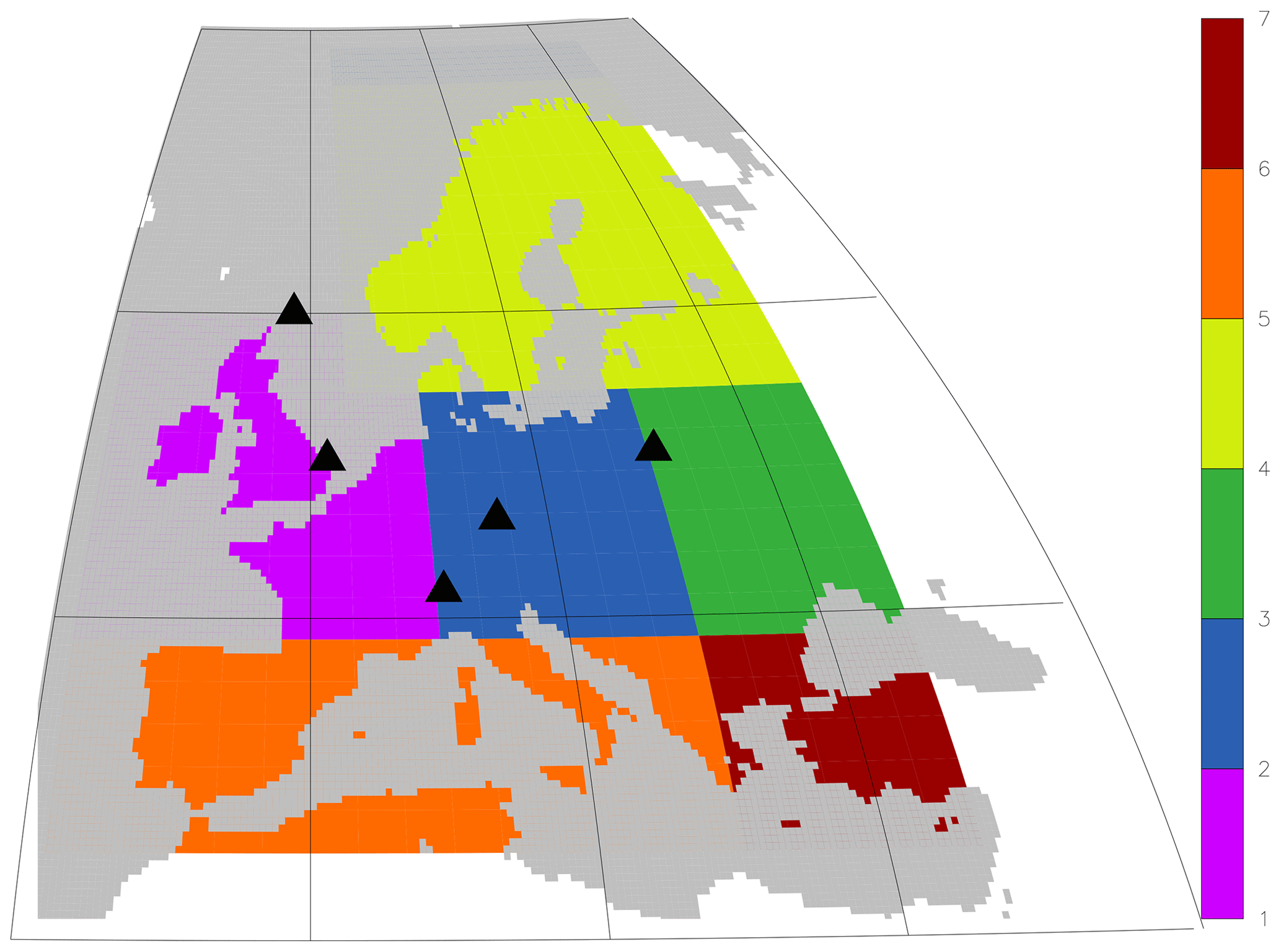
Figure 1Symbols: locations of the European APO measurement stations used in the APO inversion (set B; see Table 1). Colours: regions over which the estimated gridded FF fluxes are integrated for time series figures (“western Europe”: magenta).
2.1 The APO flux – definition and contributions
The original definition of APO as a conceptual atmospheric tracer by Stephens et al. (1998) combines measurements of the atmospheric O2 and CO2 abundances. To very good approximation, this definition can be translated into the notion of a surface–atmosphere APO flux:
(Appendix A of Rödenbeck et al., 2008). Here, and are the surface–atmosphere fluxes of O2 and CO2, respectively. The last term of Eq. (1) represents a small contribution proportional to the surface–atmosphere nitrogen flux (involving the reference mole fractions X0 of O2 and N2 in air), arising because the atmospheric O2 abundance is reported as a molar ratio of O2 to N2. The only relevant N2 flux originates from the ocean due to solubility variations with temperature.
The total surface–atmosphere O2 and CO2 fluxes comprise contributions by fossil-fuel burning (, ), the terrestrial biosphere (, (net ecosystem exchange)), and the ocean (, ). The contributions by fossil-fuel burning and by the terrestrial biosphere occur in stoichiometric proportions denoted by
and
respectively. Their contributions to the total APO flux thus are
and
(both processes are not associated with any N2 flux). To the extent that the terrestrial biospheric stoichiometry is (Severinghaus, 1995), the contribution according to Eq. (5) vanishes. This leaves the fossil-fuel APO flux as the only contribution on land and thus makes it accessible to inverse estimation based on atmospheric APO data over continents.
2.2 Atmospheric APO inversion
We use an extension of the APO inversion presented in Rödenbeck et al. (2008). As mostly done in atmospheric inversion calculations (Newsam and Enting, 1988), the surface–atmosphere flux field f is estimated by minimizing the mismatch between the measured atmospheric tracer abundance and the corresponding abundance simulated by an atmospheric tracer transport model using f. The mismatch is gauged by a quadratic cost function. The cost function also contains Bayesian a priori contributions meant to regularize the inversion, akin to Ridge regression (Hoerl and Kennard, 1970). Here we use the CarboScope inversion software described in Rödenbeck (2005, updated).
As the APO inversion of Rödenbeck et al. (2008) was targeting the sea–air oxygen flux, it had degrees of freedom to adjust only. All other contributions to the total APO flux (, , , ) had been prescribed. In particular, the FF CO2 emissions had been taken from a bottom-up inventory, and the corresponding FF O2 consumption had been calculated from the CO2 emissions assuming a constant global (Keeling, 1988). Here, this APO inversion of Rödenbeck et al. (2008) has been extended by
-
using a more realistic (in particular, spatially and temporally explicit) FF stoichiometry αFF, calculated via Eq. (2) from the inventory-based a priori and fields;
-
adding some degrees of freedom (DoF) to adjust the fossil-fuel emissions in Europe as detailed below;
-
adding observational records from European continental stations (Sect. 2.3); and
-
for inversions of real data, using a regional transport model with higher resolution over Europe, nested into the global inversion (Appendix A).
The a priori and fields are taken from GridFEDv2022.2 (Jones et al., 2022), which uses fuel-type specific oxidative ratios as in Steinbach et al. (2011) to obtain the O2 consumption from the CO2 emissions. The additional DoFs scale the fossil-fuel fluxes on land away from their a priori values (fossil-fuel emissions over the ocean, being much smaller than those on land, are not scaled). Both and are scaled by the same factors, such that the FF stoichiometry αFF of the a posteriori estimate remains identical to that of the prior. The adjustable scaling factors are allowed to vary in space (with an isotropic correlation length scale of about 380 km) and in time (with a correlation length scale of about a year (filter “Filt1T” in CarboScope notation); the yearly timescale means that the seasonal and any faster variations of the prior remain essentially unchanged). The scaling of the fossil-fuel fluxes is only done within Europe west of 35∘ E and north of 33∘ N (coloured area in Fig. 1). We verified that the results for the European fossil-fuel fluxes presented in this paper do not appreciably depend on whether or not the inversion set-up also includes any DoFs to scale the non-European fossil-fuel emissions (tests not shown). APO fluxes in non-European land regions cannot be constrained anyway because almost no continental APO data exist outside of Europe so far.
Further technical details of the APO inversion are given in Appendix A.
2.3 APO data
The APO inversion has been constrained by data from a set of global stations (referred to as set A, Table 1) plus additional stations in central and north-western Europe (set B). The locations of the European stations can be seen in Fig. 1 (symbols).
Table 1Monitoring stations measuring atmospheric O2 and CO2 abundance used in the APO inversions presented here. Stations have been grouped into sets A, B, C, and D, and ordered within each set by either latitude or longitude.
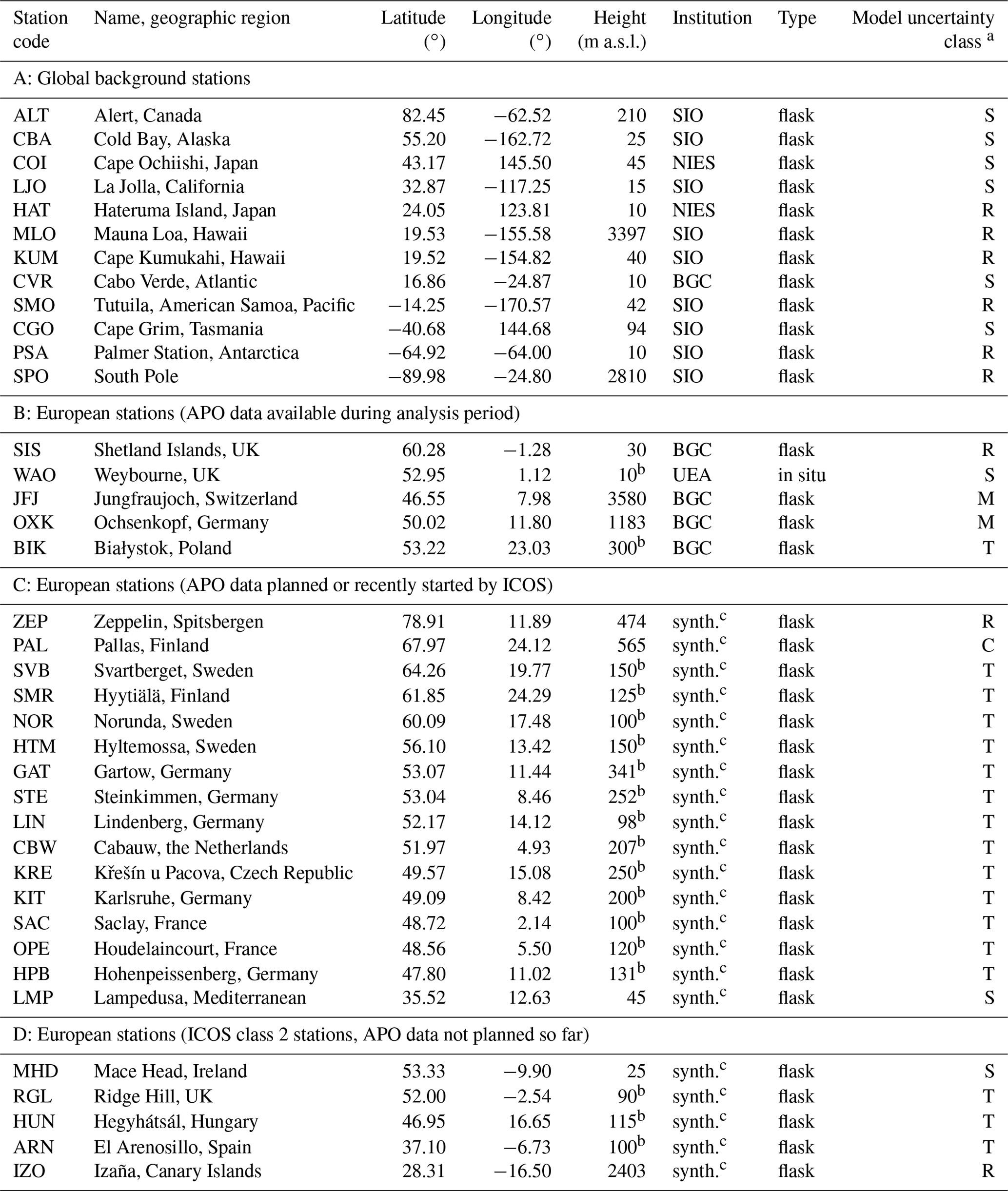
a Model uncertainty class (C – continental, M – mountain, R – remote, S – shore, T – tower; see Appendix A). b Height above ground. c Using synthetic data only; BGC: Max Planck Institute for Biogeochemistry, NIES: National Institute for Environmental Studies (Tohjima et al., 2019), SIO: Scripps Institution of Oceanography, UEA: University of East Anglia (Adcock et al., 2023).
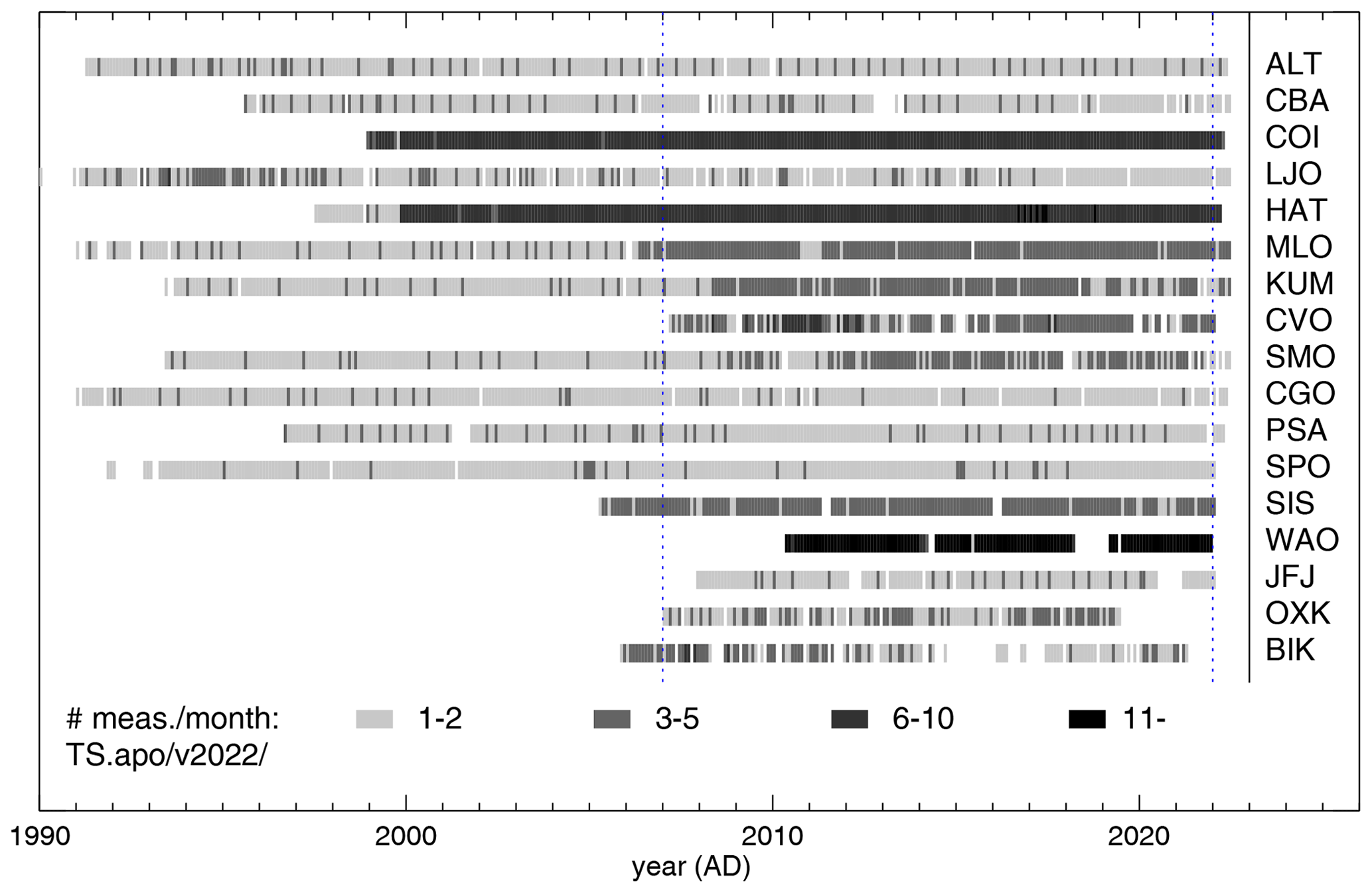
Figure 2 shows the periods over which APO data are available. The blue vertical dotted lines delimit the analysis period 2007–2021 (inclusive) of this study, chosen to comprise the years when essentially all stations have data, such that temporal variations can be constrained. The influence of gaps in the data records (such as the record at WAO starting mid 2010 or at OXK ending mid 2019) is assessed by additional model runs omitting the individual stations in turn.
Most stations provide flask measurements about once per week. Where hourly in situ time series are available (here only at WAO), only daytime values (11:00–17:00 LT) have been used, because during this time the atmospheric transport model is expected to have lowest uncertainty as the atmospheric boundary layer is well-mixed.
In order to jointly use the APO data from different laboratories in the inverse calculation, and to account for some measurement issues, some data selection or adjustment was necessary, as motivated and described in Appendix B.
2.4 Diagnostics
In order to test to what extent the decadal trend in FF CO2 emissions can be estimated by the APO inversion independently of the trend already present in the bottom-up inventory used as a prior, we performed test inversions using a manipulated (counterfactual) prior
with a scaling factor increasing linearly by β= 1 % yr−1 starting at t0= 1 January 2007. The increase has been chosen such that the decadal emissions reduction in western European is partly compensated. The oxygen consumption is scaled in the same way, such that the stoichiometry αFF of the manipulated prior is identical to that of the original prior. Due to the manipulation, after 10 years (on 1 January 2017, towards the end of our analysis period) the counterfactual prior has emissions 10 % higher than the original FF inventory. We will consider to what extent the inversion is able to compensate this scaling on the basis of the information in the APO data.
The manipulated prior has mainly been used in synthetic inversions. These are based on pseudo-data effectively created by a forward transport model simulation from the original a priori fluxes, to be compared with the original a priori fluxes as a “known truth”. As a complement, we also ran test inversions (based on the real data) using the manipulated prior, to be compared with the results of the main inversion using the original prior.
3.1 FF emissions estimated from available APO data
The dark blue line in Fig. 3 represents the results of our base APO inversion, scaling the CO2 emissions of the bottom-up inventory (black) based on the APO data from station sets A + B (Table 1, symbols in Fig. 1). Similarly, the other colour lines show inversion results where the APO data from each individual station in set B were discarded in turn.
On the year-to-year timescale, the inversion estimates contain considerably more variations than reported in the FF inventory. If taken at face value, this would suggest corrections clearly exceeding the expected uncertainty of the inventory. However, the set of runs reveals that most year-to-year features only depend on a single one of the measurement stations. For example, the steeper decreasing trend after about 2016 solely depends on the signals from the WAO station, while the lower fluxes at the beginning of the period and in about 2012 decisively depend on the OXK station. The variability is unlikely to be caused by the incomplete data coverage (Fig. 2) because large anomalies also exist within 2011–2018 when the data records are mostly available. The large variability calls for great care in interpreting the CO2 emissions estimated from the currently available data.
Concerning decadal trends, the large year-to-year variability currently precludes calculating a statistically significant trend. Even if calculating a temporal slope anyway, we find a strong dependence on the chosen stations.
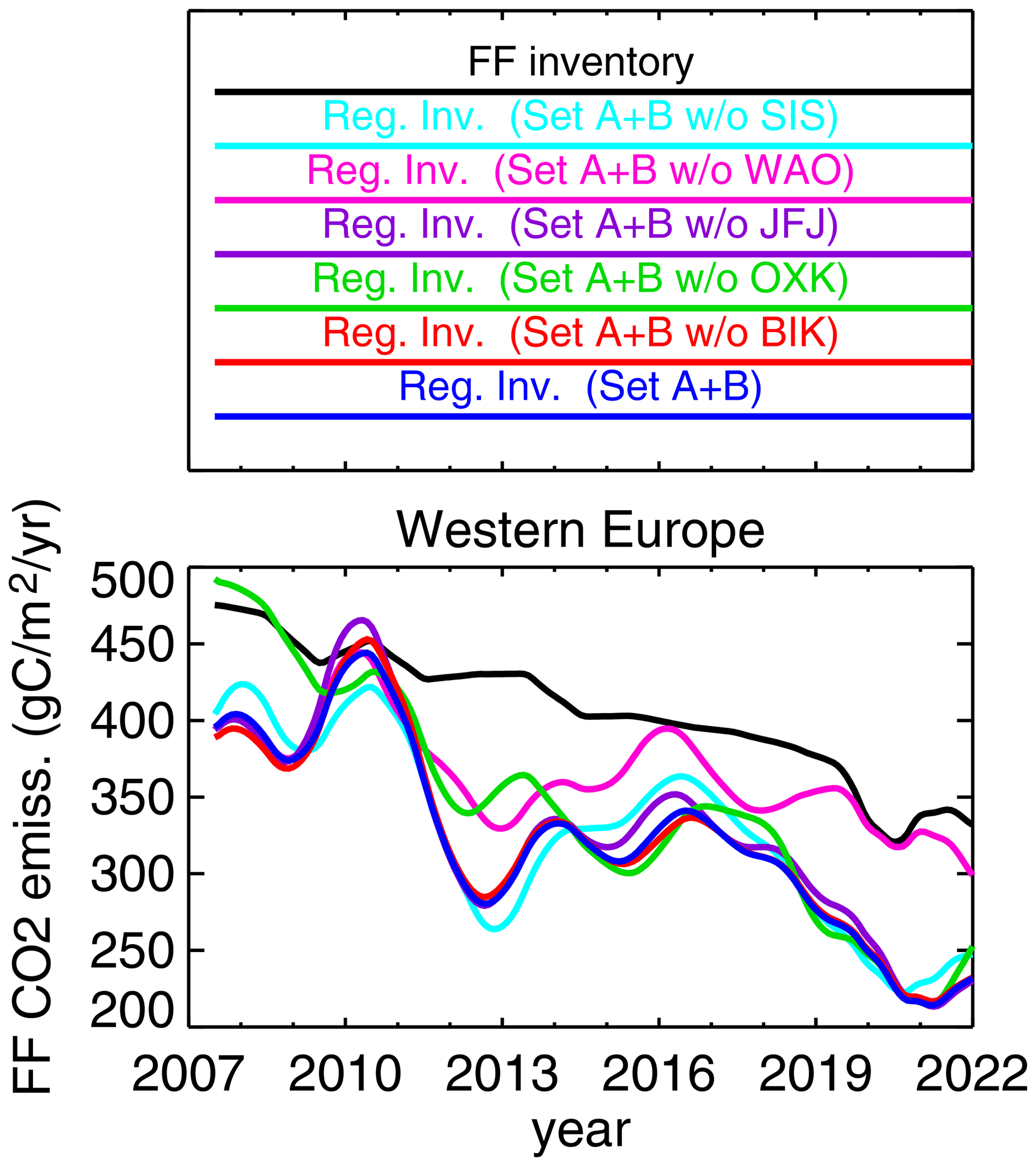
Figure 3Estimated interannual variations in the FF emissions (deseasonalized by running annual averaging and further smoothed on a 3-monthly scale) integrated over the “western Europe” region of Fig. 1. Dark blue shows the results of the regional APO inversion based on station set A + B, while the other colour lines omit individual stations of set B (see Table 1). Black shows the original FF inventory used as a prior.
The strong dependence of flux variability on individual stations may reflect local signals spuriously interpreted as regional signals, as well as measurement errors, transport model errors, or gaps in the data records. Transport model errors are generally found to play a substantial role based on various intercomparisons in the literature (e.g. Monteil et al., 2020; Munassar et al., 2023). Indeed, the results of the global inversion (Appendix A1, results not shown) differ considerably from those of the regional inversion (Appendix A2, Fig. 3), their difference mainly being the transport model.
Trying to disentangle the possible error influences, we next investigate whether the information content of the data and the degrees of freedom built into the inversion set-up would in principle allow us to estimate decadal trends in the European fossil-fuel emissions.
3.2 The potential of available and additional APO measurement stations
Because of the very small network of currently available stations with APO data, we assessed the potential of several station sets using inversions with synthetic data. As synthetic inversions do not involve measurement or model errors, they isolate the effects of data information content and degrees of freedom. The synthetic inversions start from a manipulated (counterfactual) prior described in Sect. 2.4 and try to reconstruct the bottom-up inventory (“known truth”) through the information contained in the synthetic data.
According to Fig. 4, the station set A + B can reduce the gap between the counterfactual prior (grey) and the “known truth” (black) in western Europe by more than a third (solid blue). This is consistent with the behaviour of the real-data inversion if starting from the counterfactual prior as well: the difference in a posteriori estimates is reduced by about the same factor compared to the difference in prior (tests not shown). In contrast to station set A + B, a synthetic inversion with set A alone does not move the result away from the counterfactual prior (test not shown).
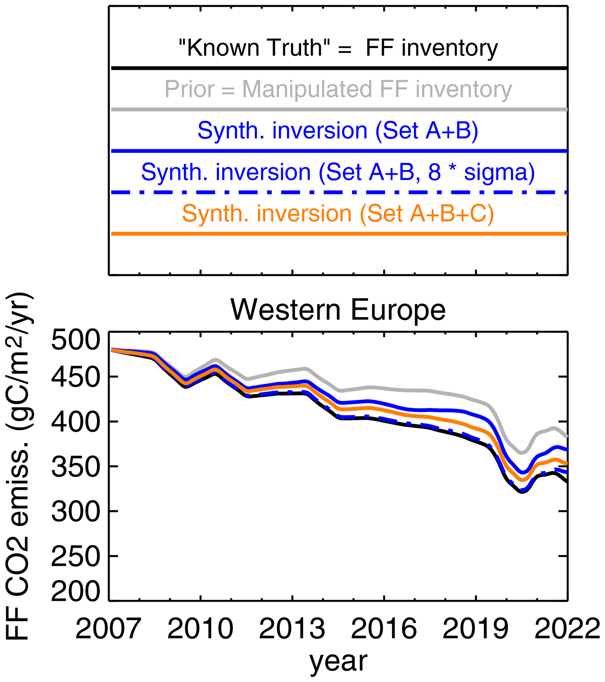
Figure 4Synthetic-data test: starting from a counterfactual prior with less emissions reduction (manipulated FF inventory defined in Sect. 2.4, grey) the synthetic inversions try to reconstruct the “known truth” (original FF inventory, black) from pseudo-data created by an atmospheric transport simulation for the same locations and times as the real data. The colour lines represent synthetic APO inversions using the same inversion set-up as Fig. 3 (solid) or a less regularized set-up (8-fold a priori uncertainty of the fossil-fuel-related degrees of freedom) having more freedom to match the data (“8-fold sigma”, broken). The colour hue indicates the station set used.
While Fig. 4 considers the average over the western European region, parts of this area may in fact be better constrained. To investigate this, Fig. 5 shows the local metric
where denotes the “known truth” identical to the normal prior, the manipulated (counterfactual) prior, and the synthetic estimate. By construction, this metric equals 100 % at pixels where the estimate fully reconstructs the “known truth” despite the deviation of the prior (indicating full constraint), and drops towards zero where the estimate remains close to the prior (indicating absence of data constraint). The metric has been calculated from yearly averaged fluxes at the test time tx= 2017. This test time has been chosen because this is the most recent year with more or less complete data coverage at the European station set B (see Fig. 2). In the base case (station set A + B and standard uncertainty settings), Fig. 5a reveals that the strongest constraint (ϱ≈ 50 %) is found in the area in between the stations of set B. This is expected because it is the gradients between the stations that determine the fluxes at any location. However, ϱ may also be enhanced there because of the large FF emissions in this same area, which allow the inversion to achieve a particularly large change in fluxes for the same change in scaling factors; indeed we find somewhat larger ϱ values in the same area even if only one of the stations has been used (additional tests not shown).
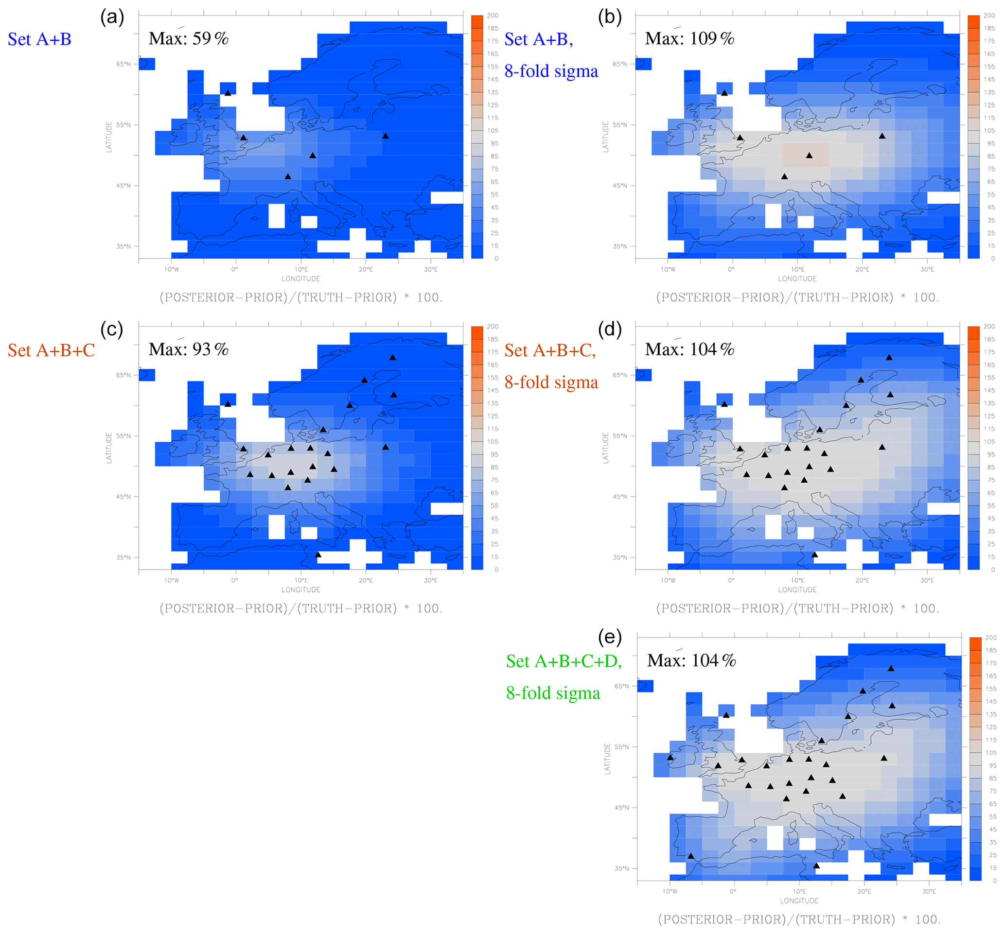
Figure 5Maps of the agreement ϱ of the synthetic inversions as in Fig. 4 with the “known truth”, relative to the difference between the “known truth” and the prior (Eq. 7). Values around 100 % (grey) indicate complete correction of the counterfactual prior. The black symbols indicate the European APO measurement stations used in the respective run.
The synthetic-data inversions also allow testing inversion set-ups with less regularization, such that the FF emissions have more freedom to be adjusted to match the atmospheric data. Such a set-up could not be used with the real data so far, because the increased freedom leads to even larger year-to-year variations than in Fig. 3, being even less likely to be true (not shown). As the synthetic-data inversions are less affected by transport model errors, measurement errors, or local signals, however, they do not have this problem. As shown by the broken blue line in Fig. 4, a synthetic-data inversion with increased freedom is better able to reconstruct the “known truth” from the data: multiplying the a priori uncertainty of the DoFs adjusting the FF fluxes by 8 (“8-fold sigma”) already matches the “known truth” almost completely in the regional average over western Europe. This confirms that there should be no fundamental obstacle against estimating FF emissions in European subregions from a logistically feasible set of atmospheric stations like set B.
In the spatially explicit view of Fig. 5b, using the more free inversion set-up (8-fold sigma) is seen to achieve essentially perfect reconstruction (ϱ≈ 100 %) almost everywhere in between the stations of set B. Some pixels slightly above 100 % compensate others slightly below 100 %, as the data can only constrain the sum of fluxes along the path of the air from station to station.
The synthetic-data inversions further allow assessing how the constraint could be improved by additional stations from which APO data are not yet available. We test a set C of European stations where APO measurements have recently been started by the Integrated Carbon Observation System (ICOS) infrastructure but are not yet available over a period sufficiently long for the inversion. In the synthetic inversion, we assume that data at the stations of set C were already available throughout the inversion calculation (one flask on day 5, 10, 15, 20, 25, and 30 of each month, local noon). The additional stations clearly improve the match in the western European FF emissions estimates, even for the tighter regularization of the standard set-up (Fig. 4, orange). In the area surrounded by the highest station density, the local constraint reaches 100 % (Fig. 5c).
In the less regularized set-up (8-fold sigma), the additional stations of set C slightly further homogenize the match in space (Fig. 5d compared to b). The additional stations located further away (Scandinavia, Mediterranean) extend the constrained area, though the gain in power to match the “known truth” seems to stay behind the central area. Possibly, the geometry of the station set C in northern and southern Europe does not sufficiently embrace larger emissions hotspots by covering upwind and downwind locations, as it does not have much west–east coverage at any given latitude. However, the smaller gain in ϱ may also just reflect the lower FF emissions (see above). The more freedom is given to the inversion, the better the performance is also in these areas (not shown). Adding further stations outside the geographical range of set C (station set D consisting of ICOS class 2 stations where APO measurements are not yet planned, Fig. 5e) similarly extends the better-constrained area towards Wales and the Iberian Peninsula.
As a general pattern in the various synthetic inversion results, the addition of stations and the decrease in regularization strength have roughly similar effects. This is also because additional data also exert a greater total power in the cost function. From our present results, therefore, we cannot yet make firm statements on a desirable station density. Such statements would also depend on the actual heterogeneity of the FF emissions signals, which in turn would need to be reflected properly in the chosen a priori spatial correlation lengths in the inversion calculation (here we only picked a correlation length rather arbitrarily). A deeper investigation seems only possible in a few years from now when multi-year time series observed at the stations of set C will be available.
As the ocean fluxes in the “known truth” have been chosen identical to the ocean prior (Sect. 2.4), any deviations of the a posteriori ocean fluxes away from the prior are spurious signals misattributed from land where prior and “known truth” are different. Among our synthetic-data inversion runs with different station sets and uncertainty settings, those that reconstruct the FF fluxes on land less well also deviate more in their ocean APO fluxes (not shown). Further, in test inversions where the ocean fluxes are fixed, the FF fluxes can be reconstructed more easily (test not shown; note that such inversions are unrealistic as they pretend the ocean flux to be known). Both these findings illustrate the presence of a posteriori anti-correlations between the errors of land and ocean fluxes, limiting the capability to correctly attribute the atmospheric APO signals to land or ocean. This means that part of the variability in Fig. 3 may also be misattributed ocean variability. The situation is consistent with forward transport simulations by Chawner et al. (2023), who find the influence of oceanic APO signals at UK stations including WAO to partially be as strong as the signals related to FF emissions. (An incomplete capability to separate land and ocean fluxes is also a widely known limitation of global atmospheric CO2 inversions where station-to-station gradients tend to span both land and ocean, Peylin et al., 2013.) As confirmed by the expansion of the well-constrained area in between the stations in Fig. 5, the availability of more and more continental stations alleviates this dependence on the ocean flux, because the inversion can more and more rely on APO gradients within the continent being less influenced by the ocean fluxes.
3.3 Uncertainties related to the O2:CO2 stoichiometry of FF emissions
The APO data primarily constrain the FF-related APO flux . In our inversion algorithm, this APO flux is linked in a fixed way to the FF CO2 emissions via Eq. (4) using the O2:CO2 stoichiometry αFF,pri as given in the bottom-up inventory. We can however re-compute the FF CO2 emissions from the estimated APO flux under the assumption of modified stoichiometries αFF,mod by
In the uncertainty assessment of this section, we used the inventory as a proxy for an APO inversion result, as the actual inversion results of Fig. 3 seem too noisy for this purpose.
Figure 6 compares the FF CO2 emissions as it would directly come from the APO inversion using the original O2:CO2 stoichiometry αFF,pri (solid blue) with recomputed FF CO2 emissions assuming constant stoichiometries αFF,mod of −1.50 (green) or −1.55 (cyan), respectively. We first notice that the solid blue line roughly agrees with the green one in the earlier years but approaches and even crosses the cyan line in the later years. This reflects that the FF stoichiometry αFF,pri according to the bottom-up inventory (in a flux-weighted average sense for “western Europe”) changed from about −1.50 to beyond −1.55 over the course of our analysis period, compatible with the increasing share of natural gas in the fuel mix. It also shows, however, that a shift in the assumed FF stoichiometry αFF by the same 0.05 difference would alter the inferred FF CO2 emissions by an amount more than half of the emissions reduction over this period. As noted above, this alteration in the CO2 emissions estimate occurs despite the estimated APO flux being identical for all three lines of Fig. 6. This means that the FF stoichiometry αFF,pri and its temporal changes need to be known to an uncertainty well below 0.05.
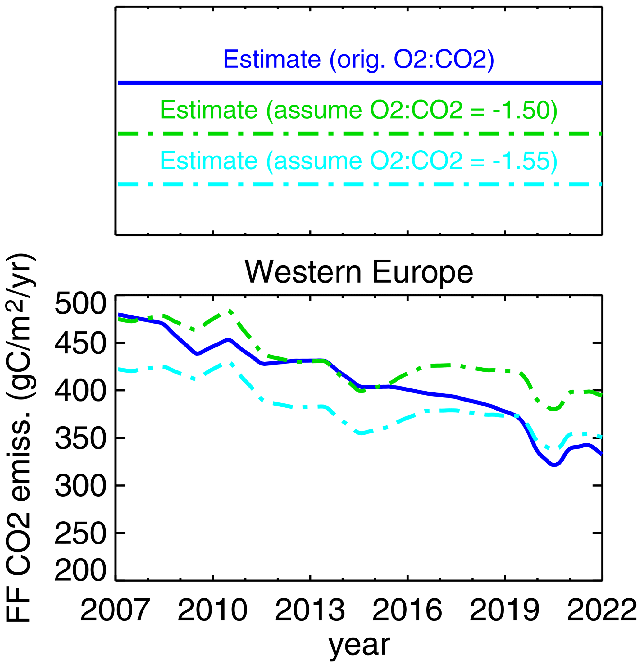
Figure 6Importance of the O2:CO2 stoichiometry of FF emissions (αFF,pri) used in the APO inversion: a given FF CO2 emissions estimate based on the original time and space varying αFF,pri from the bottom-up inventory (blue, here using the FF inventory as a proxy for an inversion result) is compared to CO2 emissions re-computed from the corresponding APO flux assuming constant stoichiometries of −1.50 (green) or −1.55 (cyan), respectively.
3.4 Uncertainties related to the O2:CO2 stoichiometry of exchanges from the land biosphere
According to Eq. (5), the APO flux associated with photosynthesis and respiration on land vanishes only if the stoichiometry is exactly αNEE= −1.1 as assumed in the APO definition (Stephens et al., 1998). However, recent measurements of atmospheric O2 and CO2 variations closer to or within the canopy suggest that the actual stoichiometry αNEE may be smaller in absolute value and depend on time of day and vegetation state (e.g. Seibt et al., 2004), even though it remains unclear what this means for the large-scale effective stoichiometry relevant here. As the APO data constrain the sum of all surface–atmosphere APO fluxes, any presence of a non-zero would lead to a compensating bias , which translates into a bias
in the estimated FF CO2 emissions. We calculated this bias for an assumed biospheric stoichiometry , using (the approximate current value for “western Europe”; see Sect. 3.3) and an NEE flux field estimated from atmospheric CO2 data (CarboScope atmospheric CO2 inversion s10oc_v2022, update of Rödenbeck et al., 2018).
Again using the inventory as a proxy for an APO inversion result, Fig. 7 compares the estimated FF CO2 emissions without (blue) and with (green) this bias added. On the yearly timescale (Fig. 7a) mainly considered in this study, the bias only leads to a small shift compared to the year-to-year variations or decadal trend. Therefore, uncertainties in the biospheric O2:CO2 stoichiometry on the order of 0.05 should not be problematic in the APO-based estimation of yearly FF CO2 emissions and their trend.
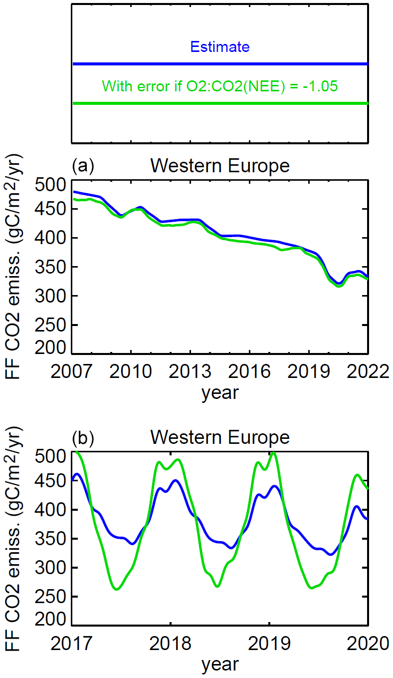
Figure 7What if the true O2:CO2 stoichiometry of terrestrial biosphere was −1.05, rather than −1.1 as assumed in the APO definition? For a given FF CO2 emissions estimate (blue, here using the FF inventory as a proxy for an inversion result), the difference between the green and blue lines represents the corresponding error as calculated from Eq. (9). (a) Yearly fluxes as in Fig. 3; (b) fluxes on the original daily time resolution for 3 example years.
For seasonal variations however (Fig. 7b), due to the large seasonal cycle of NEE, the impact of the associated bias turns out to be as large as the signal itself. To the extent that the chosen shift in the biospheric O2:CO2 stoichiometry by 0.05 represents its uncertainty, this implies that our APO-based estimates cannot make any meaningful statements on the seasonality of FF CO2 emissions. (If the real O2:CO2 stoichiometry of NEE significantly changed with seasons, there might additionally be some rectification of the seasonal NEE bias, which could even have an effect on the yearly mean bias. We do not know so far whether this is the case.)
Many of the results presented here are encouraging regarding the use of APO data to constrain yearly FF CO2 emissions in European subregions. Our inversions with synthetic data demonstrate that a logistically realistic set of stations suffice to constrain large-scale emissions including decadal trends (Sect. 3.2). Though the actual O2:CO2 stoichiometry αNEE of land-biospheric fluxes may deviate from the value of 1.1 assumed in the APO definition (see Eq. 1) and rather be in the range of 1.0 to 1.1 and possibly beyond (see a summary of values in Keeling and Manning, 2014), this does not seem to pose a fundamental obstacle on the yearly timescale (Sect. 3.4); nevertheless, a better characterization of αNEE on the space and timescales relevant here would be useful for accurate FF emission estimation from APO data.
More problematically, uncertainties in the O2:CO2 stoichiometry αFF of the FF emissions need to be well below 0.05 on the regional scale (Sect. 3.3). Keeling and Manning (2014) (their Table 2) give uncertainties of the O2:CO2 stoichiometry for individual fuel types of ±0.03 or ±0.04. In the αFF values used here, calculated from the CO2 and O2 fluxes from the bottom-up inventory, there is additional uncertainty related to possible errors in the fuel mix. Thus, more work is needed to determine the O2:CO2 stoichiometry of FF emissions sufficiently accurately.
The largest problem to date are strong interannual variations implied by the APO data available within Europe for the past 1–2 decades (Sect. 3.1). Even in our standard APO inversion set-up where adjustments of the FF emissions are regularized so strongly that – according to our synthetic inversion – it becomes difficult to constrain trends, the implied interannual variations still exceed the expected uncertainty of the bottom-up inventory. We therefore consider these strong interannual variations as spurious. Unfortunately, they mostly mask the information on decadal trends.
As in any atmospheric inversion, spurious interannual variations could conceivably arise from systematic time-dependent measurement or transport model errors or from small-scale signals being interpreted by the inversion as regional signals. If systematic measurement errors or local signals played a role, we would expect them to depend on the use of specific stations. Indeed, we did not find much coherence between the variations inferred from the small number of existing European stations (Sect. 3.1). Unfortunately, despite our attempts for example looking at the model–data residuals of the inversion runs using different station sets, we did not find any specific clues how to tackle this problem.
We expect that clearer answers can be given as soon as the upcoming or recently started APO data from the ICOS stations (set C) cover several years. To the extent that the variations reflect random errors in data and transport model, the larger station set will help to average these out. Possibly, the availability of more stations will also allow us to establish the reliability of the variations by confirming that they are resolved using different independent combinations of stations (as in Rödenbeck et al., 2008). This approach requires redundancy in the network, i.e. the ability of different combinations of stations to resolve fluxes over essentially the same domain. Unfortunately, the coverage at present is too sparse.
A larger set of APO measurement stations will also more adequately represent the spatial heterogeneity of FF emissions and their trends. In our tests based on a counterfactual prior, we only implemented a spatially uniform deviation from the original inventory. In reality, the decadal trends of FF emissions are spatially very inhomogeneous (not shown) reflecting the build-up or decommissioning of industrial infrastructure in the course of time. Consequently, the errors of bottom-up inventories may also be expected to be spatially heterogeneous, as the proxy data used to disaggregate country totals will not perfectly reflect such changes. By neglecting this heterogeneity, our tests pose an easier challenge to the inversion. The issue should be revisited in the light of the upcoming more dense station network in a few years from now. Such work should also include tests to find out which spatial and temporal correlations are appropriate to be implemented in the inversion set-up, as a denser station network may allow constraining degrees of freedom on a less coarse spatial resolution. We note that this situation also applies in general to other top-down methods for FF quantification, such as radiocarbon. This means that development work regarding any of these tracers may have co-benefits for other tracers as well.
By using a flux representation on daily time steps, our calculation neglects possible complications related to diurnal variations. Diurnal co-variations in fluxes and atmospheric transport may lead to biases also on longer temporal scales (often called “rectification effects”). Similarly, biases may arise from diurnal co-variations in fluxes and the oxidative ratios (αFF or αNEE). Unfortunately, there is no easy solution, because the diurnal variations in most fluxes and oxidative ratios can neither be inferred from the atmospheric data nor are they well known a priori. More work is needed to quantify and possibly correct the impact of the diurnal rectification effects on the FF emissions estimates. However, regarding decadal trends as targeted in this paper, these effects may be less problematic to the extent that the diurnal variations stay similar over time.
Regarding CO2 emissions from cement production, these emissions are somewhat special among the anthropogenic emissions as there is no associated O2 consumption. However, as they are part of the bottom-up inventory, they are properly reflected in the overall stoichiometry αFF used here. In Europe, the share of cement production in the total anthropogenic CO2 emissions is low anyway; however this issue may need more attention for APO-based studies in other parts of the world.
A possible complication in future uses of continental APO data may be the production of hydrogen (H2) as a fuel, as the electrolysis of water also produces O2. Though the same amount of O2 is consumed later in H2 oxidation during fuel use, its location will generally differ from that of H2 production and thus have an impact on the APO observations.
From the assessments presented here we conclude that the estimation of decadal trends in fossil-fuel CO2 emissions in subcontinental regions from sustained APO measurements on at least weekly frequency should be feasible in practice. Even though our estimates based on a small number of existing measurement locations involved too large apparent year-to-year variations to infer decadal trends, more stable estimates seem possible as soon as a denser network of APO observations over several years become available. We therefore believe that ongoing measurement efforts, including those recently started within the European ICOS research infrastructure, are valuable investments in future capabilities to independently verify fossil-fuel CO2 emissions inventories.
Although this study is only considering fluxes within Europe, the inversion of atmospheric data is an intrinsically global problem. Due to the computational requirements, global inversions as in Rödenbeck et al. (2008) are limited to relatively coarse resolution of the atmospheric tracer transport simulation, involving relatively large model errors. Regional inversions offer a way to increase the resolution within the target region, however at the cost of additional complexity to properly transfer the global signals across the regional boundary. As a further problem, if simulating the regional atmospheric transport via pre-computed “footprints” as done here (see Appendix A2), additional hypothetical data points as in our synthetic inversions cannot easily be included. Therefore, all synthetic inversions (Figs. 4 and 5, being not very sensitive to transport errors anyway) have been done as global calculations in this study, while the results using real APO data (Fig. 3) have been refined by regional nesting.
A1 Global inversion
The global inversion has been done with the TM3 atmospheric transport model (Heimann and Körner, 2003) on a resolution of 5∘ longitude × about 4∘ latitude. TM3 has been driven by meteorological fields from the NCEP reanalysis (Kalnay et al., 1996). The pixel size of the global flux field is 2.5∘ longitude × 2∘ latitude.
In the previous set-up (version v2021) of the APO inversion, the a priori uncertainties of the long-term and seasonal DoFs of the oceanic APO flux had been enhanced compared to the non-seasonal interannual DoFs. This uncertainty enhancement has been removed, as it had worsened the mutual misattribution of land and ocean signals as revealed by synthetic-data tests (not shown). Using non-enhanced uncertainties for the oceanic seasonal cycle DoFs also improves the agreement with the extratropical seasonal cycles of the independent ocean O2 fluxes by Garcia and Keeling (2001) based on heat fluxes (not shown).
As in Rödenbeck et al. (2008) (and in the CarboScope inversions in general; Rödenbeck, 2005), the Bayesian uncertainty of the model–data mismatch has been chosen depending on an assumed model uncertainty class of each station (Table 1) as R (remote), 1.5 ppm; S (shore), 2.25 ppm; M (mountain), 2.25 ppm; T (tower), 4.5 ppm; and C (continental), 4.5 ppm. To this assumed model uncertainty, an assumed measurement uncertainty of 0.4 ppm is added quadratically. This value, slightly larger than in the CarboScope CO2 inversion, may seem small for APO measurements but has been kept nevertheless in light of the model uncertainty being larger and barely known anyway. Further, a “data-density weighting” (Sect. 2.3.3 of Rödenbeck, 2005) has been applied, assuming that data points within time intervals of a week may not add new information due to the temporal correlations in synoptic transport and in the flux representation. This data-density weighting also leads to comparable weights of flask or in situ stations despite their dramatically different data density.
Finally, data outliers have been removed by an “nσ selection” (similar to an “iteratively re-weighted least squares” algorithm). As described in Sect. A1.3 of Rödenbeck et al. (2018), pre-runs of the inversion based on all available data points have been done. Separately for every station, the standard deviations (σ) of the a posteriori residuals of these pre-runs have been determined, and any data point with a residual larger than nσ has been discarded in all the main inversion runs. In contrast to Rödenbeck et al. (2018), a slightly stricter threshold of n=1.5 (rather than n=2) has been used. Moreover, the selection of the individual stations of set B has been done according to separate pre-runs using station set A and only the considered station of set B. This was done in light of the partially contradicting signals from the individual stations (see Fig. 3), which would otherwise also remove data points that cannot be fit because the inversion has to compromise between the stations.
A2 Regional inversion
In order to reduce transport model uncertainty at the continental stations of set B, we also performed higher-resolution regional inversions within our target region, using the regional transport model STILT (Lin et al., 2003; Trusilova et al., 2010). The regional flux field covers 15∘ W–35∘ E and 33–73∘ N with a pixel size of 0.25∘ longitude × 0.25∘ latitude.
The regional inversion has been nested into the global inversion using the “two-step scheme” introduced in Rödenbeck et al. (2009). Each regional inversion uses the far-field contributions from a global inversion run based on the same set of stations. (In principle, one may consider to use the same far-field contributions (e.g. from a global inversion based on the maximum station set) for all regional runs. This does change the result, even though by a difference smaller than the difference between the station sets in Fig. 3 (tests not shown). We chose identical station sets in global and regional inversion runs as having the greatest mutual consistency.)
In terms of data, a priori fluxes, and uncertainties, the regional inversion is done like the global inversion. We do not perform a new “nσ” outlier detection (Rödenbeck et al., 2018) for the regional run but use the data as selected by the “nσ” outlier detection from the global runs, even though there is a chance that some data points discarded for not being well represented by TM3 can now be better represented by STILT and thus could be kept. However, using far-field contributions simulated by TM3 for these data points may also pose a risk. Unfortunately, the choice of outlier detection in the regional inversion does appreciably influence its results (tests not shown), comparable to the choice of station set in Fig. 3.
B1 Data by UEA
At WAO station (Adcock et al., 2023), all values flagged as 2 (insecure values during build-up phase until May 2010) or 3 (contamination due to a leaking pump from 1 March 2018 to 22 March 2019) have been discarded.
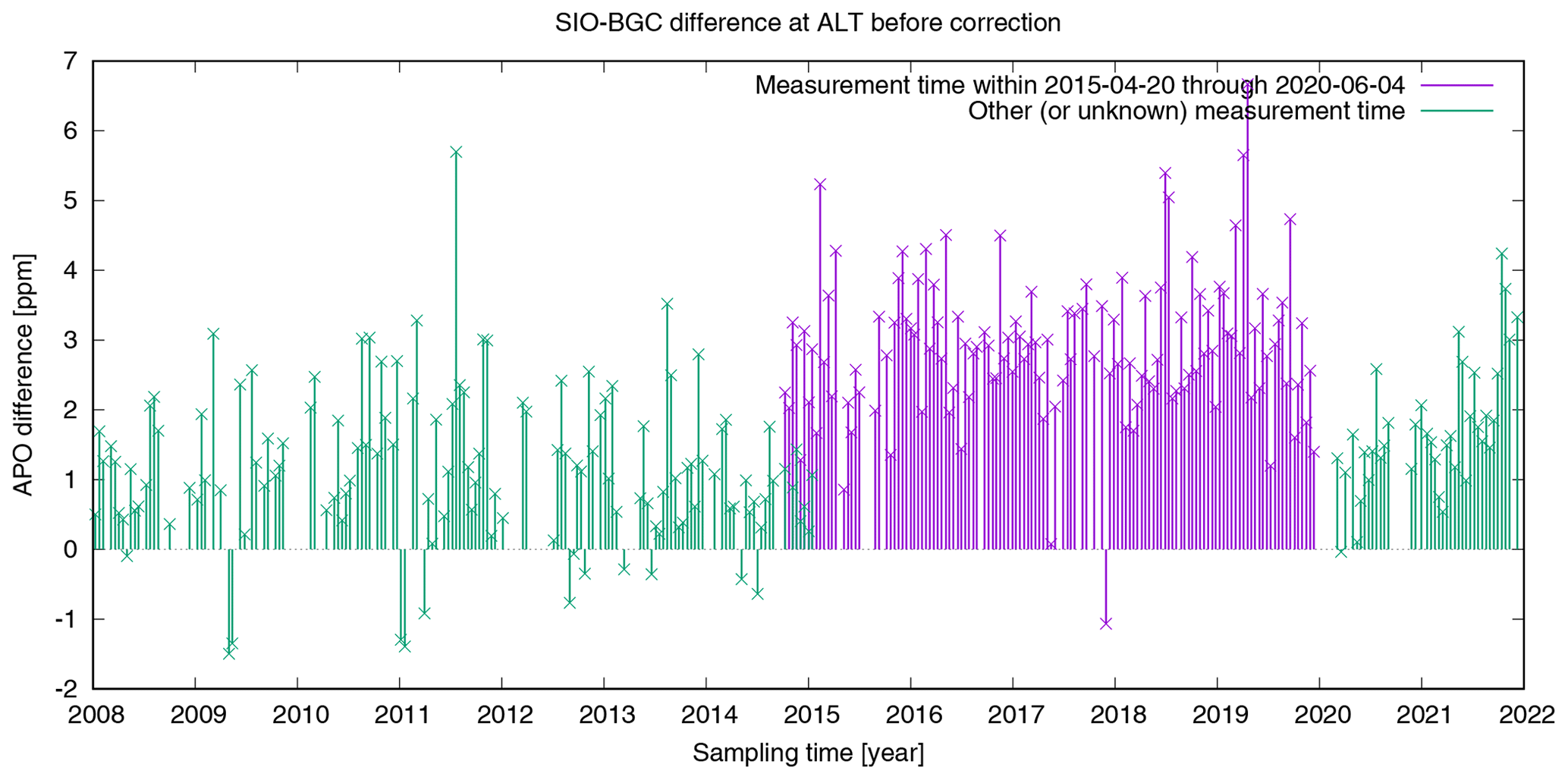
Figure B1Difference between the APO observations (flask triplet means, before additive correction) sampled simultaneously by SIO and BGC at ALT station. The triplet means of the BGC flasks have been calculated separately for flasks with measurement times within or outside the “leakage period” 20 April 2015 through 4 June 2020 (see Sect. B2 for more explanation and the corresponding correction applied).
B2 Data by BGC
In order to ensure data quality and comparability, the BGC–IsoLab measurements (see Table 1) have been compared to those done from regular simultaneous sampling by the Scripps Laboratory (SIO) at the supersite Alert (ALT). SIO is recognized as the expert laboratory for measurements within the Global Atmospheric Watch community. The comparison revealed two issues that have been addressed in the following ways:
-
The “Ar-corrected” data as described in Heimann et al. (2022) have been used. This adjustment attempts to remove influences from leakages during flask storage or from other processes that affect and in proportional ways. Indeed, the “Ar-corrected” data agree better than the uncorrected data with the simultaneous measurements by SIO at station ALT (Fig. 10 (middle panel) of Heimann et al., 2022). Of course, the Ar-based adjustment also leads to a spurious transfer of real signals from the values to the values; however, the benefit of reducing measurement artifacts seems to outweigh this problem.
-
Even after the “Ar-correction” has been applied, the BGC values still differ from the SIO values in a systematic way. We find both an overall mean difference and a rectangular-shaped enhancement (step-like changes up and back) of the difference during about 2015–2019 (Fig. B1). We attribute the overall mean difference to an offset between the Scripps scale and its local implementation through the standard gases at BGC. This offset is currently being determined by re-measuring BGC standard gases in the SIO laboratory, allowing the reduction of it in future BGC data releases. As this is an ongoing process, we use for now the SIO–BGC comparison at ALT to apply an additive correction to the BGC APO values for this paper, as described below.
The end of the period of enhanced SIO–BGC differences could be traced to the replacement of a broken autosampler valco valve in the BGC–IsoLab. Strikingly, all the BGC flasks after the anomalous period have been measured after this replacement on 8 June 2020 (see the colour coding of the difference values in Fig. B1 according to the BGC measurement date; note the delay between sampling and measurement due to the remoteness of station ALT). We therefore hypothesize that the systematically larger SIO–BGC differences were caused by a micro-leak of the valco valve that had remained unrecognized. Such a leak can adversely affect the ratios. As sample and standard gases pass the same valve, one would actually expect that the effect would cancel out through the calibration. Conceivably, however, the leak affected standards and samples in different ways, as standards are supplied by high-pressure tanks, while samples come in 1 L glass flasks. While the pressure and flow rate of the standards are kept constant, the low sample pressure (between 1.4 and 2.0 bar absolute pressure) of the sampling flasks causes a small pressure gradient, and thus flow gradient, through the valco valve during the measurement process, which requires 200 mL of sample. It is conceivable that a micro leak in the valco valve affected the sample flow subject to a pressure gradient, but not the standard gas flow that was not subject to a pressure gradient.
The assumption that the entire anomalous period was related to the same cause is supported by the behaviour of the individual flasks having been sampled at its beginning in late 2014 or early 2015. At each sampling time, generally three flasks are sampled in the BGC programme. Coincidentally, individual flasks of these triplets sampled simultaneously have been measured at times several weeks or even months apart. It turns out that flasks measured until early April 2015 tend to agree with the simultaneously sampled SIO flasks systematically better than flasks measured from early May 2015 onwards. In Fig. B1, the corresponding triplets are recognized by having two difference values for one sampling time: a lower one (green) from the flask(s) measured before 20 April 2015 and a larger one (violet) from the flask(s) measured on or after that day. Strikingly, the lower/higher difference values have a similar order of magnitude as those outside/inside the anomalous period. We therefore consider 20 April 2015 as the start date of the “leakage period” (even though the available information would also be compatible with the leak having occurred about 1 week earlier or later). The last measurements before the replacement of the valve were done on 4 June 2020, thus marking the end of the “leakage period”.
If the step changes in the SIO–BGC difference at station ALT were caused by a leaking valve rather than a specific sampling problem at this station, the data from the other BGC stations must be affected in the same way. Indeed, test inversions using set A plus the individual BGC stations (before the data correction described below has been applied) yield a similar downward drop in estimated APO fluxes within the area of influence of the respective stations (not shown).
To compensate for the effect of the leak, we split the entire set of individual flask values (for all BGC stations) into two distinct sets having been measured within or outside the “leakage period” 20 April 2015 through 4 June 2020, respectively. For these two sets, we separately calculate the mean SIO-minus-BGC difference at ALT (discarding any difference values with sampling times before 2008) and add it as a correction to all triplet means from the corresponding set (outside the “leakage period”: 1.30 ppm, inside: 2.89 ppm). Finally, we re-unify the two separate time series of each station (note that, for all stations except ALT, every flask triplet has been measured either completely within or completely outside the “leakage period”, such that we do not have to deal with handling more than one triplet mean at any given sampling time for the stations used in the inversion).
B3 Data by NIES
In order to bridge the differences in scale between NIES and SIO, the data by NIES (Tohjima et al., 2019) have been adjusted according to
The factor in the first line represents span differences, taken from the scale comparison by Aoki et al. (2021) based on measurements against a gravimetric scale. The time-dependent function in the second line represents scale drifts, obtained by linear fit to the differences between regular simultaneous measurements by NIES and SIO at La Jolla (California) from t0= 2 March 2010 through 15 May 2022.
Inversion results will be made available at https://www.bgc-jena.mpg.de/CarboScope/?ID=apo (Rödenbeck, 2023).
CR, SH, and IL conceptualized the study. KEA, ME, AJ, RFK, ACM, HM, PAP, MR, and YT were involved in the collection, analysis, and curation of the APO data from the various monitoring stations, which form the basis of this work. SM provided the “footprint” data of the STILT model. CR developed the inversion software, carried out the inversion runs, and visualized the results. All co-authors, in particular PAP and IL, took part in the analysis and interpretation of the results. CR prepared the manuscript, with important contributions from all co-authors.
At least one of the (co-)authors is a member of the editorial board of Atmospheric Chemistry and Physics. The peer-review process was guided by an independent editor, and the authors have also no other competing interests to declare.
Publisher’s note: Copernicus Publications remains neutral with regard to jurisdictional claims made in the text, published maps, institutional affiliations, or any other geographical representation in this paper. While Copernicus Publications makes every effort to include appropriate place names, the final responsibility lies with the authors.
We would like to thank all persons involved in the APO measurements. Matt Jones kindly added an O2 layer to the GridFED emissions inventory.
Atmospheric O2 and CO2 measurements at WAO were funded by the UK Natural Environment Research Council (NERC) (grant nos. NE/F005733/1, NE/I013342/1, NE/I02934X/1, QUEST010005, NE/N016238/1, NE/S004521/1, and NE/R011532/1), by the EU FP6 Integrated Project CarboOcean (grant no. 511176 GOCE), and by the UK National Centre for Atmospheric Science (NCAS) from December 2013 onward. Andrew C. Manning, Penelope A. Pickers, and Karina E. Adcock also received funding from the European Union's Horizon Europe Research and Innovation programme under HORIZON-CL5-2022-D1-02 (grant no. 101081430 – PARIS).
The article processing charges for this open-access publication were covered by the Max Planck Society.
This paper was edited by Ronald Cohen and reviewed by three anonymous referees.
Adcock, K. E., Pickers, P. A., Manning, A. C., Forster, G. L., Fleming, L. S., Barningham, T., Wilson, P. A., Kozlova, E. A., Hewitt, M., Etchells, A. J., and Macdonald, A. J.: 12 years of continuous atmospheric O2, CO2 and APO data from Weybourne Atmospheric Observatory in the United Kingdom, Earth Syst. Sci. Data, 15, 5183–5206, https://doi.org/10.5194/essd-15-5183-2023, 2023. a, b
Andres, R., Boden, T., and Marland, G.: Monthly Fossil-Fuel CO2 Emissions: Mass of Emissions Gridded by One Degree Latitude by One Degree Longitude, Carbon Dioxide Information Analysis Center, Oak Ridge National Laboratory, U.S. Department of Energy, Oak Ridge, Tennessee, USA, https://doi.org/10.3334/CDIAC/ffe.MonthlyMass.2016, 2016. a
Andres, R. J., Boden, T. A., and Higdon, D.: A new evaluation of the uncertainty associated with CDIAC estimates of fossil fuel carbon dioxide emission, Tellus B, 66, 23616, https://doi.org/10.3402/tellusb.v66.23616, 2014. a
Aoki, N., Ishidoya, S., Tohjima, Y., Morimoto, S., Keeling, R. F., Cox, A., Takebayashi, S., and Murayama, S.: Intercomparison of O N2 ratio scales among AIST, NIES, TU, and SIO based on a round-robin exercise using gravimetric standard mixtures, Atmos. Meas. Tech., 14, 6181–6193, https://doi.org/10.5194/amt-14-6181-2021, 2021. a
Calvo Buendia, E., Tanabe, K., Kranjc, A., Baasansuren, J., Fukuda, M., Ngarize, S., Osako, A., Pyrozhenko, Y., Shermanau, P., and Federici, S.: 2019 Refinement to the 2006 IPCC Guidelines for National Greenhouse Gas Inventories, IPCC, Switzerland, https://www.ipcc.ch/report/2019-refinement-to-the-2006-ipcc-guidelines-for-national-greenhouse-gas-inventories/ (last access: 18 April 2023), 2019. a
Chawner, H., Adcock, K. E., Arnold, T., Artioli, Y., Dylag, C., Forster, G. L., Ganesan, A., Graven, H., Lessin, G., Levy, P., Luijx, I. T., Manning, A., Pickers, P. A., Rennick, C., Rödenbeck, C., and Rigby, M.: Atmospheric oxygen as a tracer for fossil fuel carbon dioxide: a sensitivity study in the UK, EGUsphere [preprint], https://doi.org/10.5194/egusphere-2023-385, 2023. a
Denier van der Gon, H. A. C., Kuenen, J. J. P., Janssens-Maenhout, G., Döring, U., Jonkers, S., and Visschedijk, A.: TNO_CAMS high resolution European emission inventory 2000–2014 for anthropogenic CO2 and future years following two different pathways, Earth Syst. Sci. Data Discuss. [preprint], https://doi.org/10.5194/essd-2017-124, in review, 2017. a
Friedlingstein, P., O'Sullivan, M., Jones, M. W., Andrew, R. M., Gregor, L., Hauck, J., Le Quéré, C., Luijkx, I. T., Olsen, A., Peters, G. P., Peters, W., Pongratz, J., Schwingshackl, C., Sitch, S., Canadell, J. G., Ciais, P., Jackson, R. B., Alin, S. R., Alkama, R., Arneth, A., Arora, V. K., Bates, N. R., Becker, M., Bellouin, N., Bittig, H. C., Bopp, L., Chevallier, F., Chini, L. P., Cronin, M., Evans, W., Falk, S., Feely, R. A., Gasser, T., Gehlen, M., Gkritzalis, T., Gloege, L., Grassi, G., Gruber, N., Gürses, Ö., Harris, I., Hefner, M., Houghton, R. A., Hurtt, G. C., Iida, Y., Ilyina, T., Jain, A. K., Jersild, A., Kadono, K., Kato, E., Kennedy, D., Klein Goldewijk, K., Knauer, J., Korsbakken, J. I., Landschützer, P., Lefèvre, N., Lindsay, K., Liu, J., Liu, Z., Marland, G., Mayot, N., McGrath, M. J., Metzl, N., Monacci, N. M., Munro, D. R., Nakaoka, S.-I., Niwa, Y., O'Brien, K., Ono, T., Palmer, P. I., Pan, N., Pierrot, D., Pocock, K., Poulter, B., Resplandy, L., Robertson, E., Rödenbeck, C., Rodriguez, C., Rosan, T. M., Schwinger, J., Séférian, R., Shutler, J. D., Skjelvan, I., Steinhoff, T., Sun, Q., Sutton, A. J., Sweeney, C., Takao, S., Tanhua, T., Tans, P. P., Tian, X., Tian, H., Tilbrook, B., Tsujino, H., Tubiello, F., van der Werf, G. R., Walker, A. P., Wanninkhof, R., Whitehead, C., Willstrand Wranne, A., Wright, R., Yuan, W., Yue, C., Yue, X., Zaehle, S., Zeng, J., and Zheng, B.: Global Carbon Budget 2022, Earth Syst. Sci. Data, 14, 4811–4900, https://doi.org/10.5194/essd-14-4811-2022, 2022. a
Garcia, H. E. and Keeling, R. F.: On the global oxygen anomaly and air-sea flux, J. Geophys. Res., 106, 31155–31166, 2001. a
Heimann, M. and Körner, S.: The global atmospheric tracer model TM3, Tech. Rep. 5, Max Planck Institute for Biogeochemistry, Jena, Germany, https://www.bgc-jena.mpg.de/5362450/tech_report05.pdf (last access: 18 April 2023), 2003. a
Heimann, M., Jordan, A., Brand, W., Lavric, J., Moossen, H., and Rothe, M.: The atmospheric flask sampling program of MPI-BGC Version 13, 2022, Max Planck Institute for Biogeochemistry, Jena, Germany, https://doi.org/10.17617/3.8r, 2022. a, b
Hoerl, A. E. and Kennard, R. W.: Ridge Regression: Biased Estimation for Nonorthogonal Problems, Technometrics, 12, 55–67, https://doi.org/10.2307/1267351, 1970. a
Janssens-Maenhout, G., Crippa, M., Guizzardi, D., Muntean, M., Schaaf, E., Dentener, F., Bergamaschi, P., Pagliari, V., Olivier, J. G. J., Peters, J. A. H. W., van Aardenne, J. A., Monni, S., Doering, U., Petrescu, A. M. R., Solazzo, E., and Oreggioni, G. D.: EDGAR v4.3.2 Global Atlas of the three major greenhouse gas emissions for the period 1970–2012, Earth Syst. Sci. Data, 11, 959–1002, https://doi.org/10.5194/essd-11-959-2019, 2019. a
Jones, M. W., Andrew, R. M., Peters, G. P., Janssens-Maenhout, G., De-Gol, A. J., Dou, X., Liu, Z., Pickers, P., Ciais, P., Patra, P. K., Chevallier, F., and Le Quéré, C.: Gridded fossil CO2 emissions and related O2 combustion consistent with national inventories 1959–2021, Zenodo [data set], https://doi.org/10.5281/zenodo.7016360, 2022. a, b
Kalnay, E., Kanamitsu, M., Kistler, R., Collins, W., Deaven, D., Gandin, L., Iredell, M., Saha, S., White, G., Woollen, J., Zhu, Y., Chelliah, M., Ebisuzaki, W., Higgins, W., Janowiak, J., Mo, K. C., Ropelewski, C., Wang, J., Leetmaa, A., Reynolds, R., Jenne, R., and Joseph, D.: The NCEP/NCAR 40-year reanalysis project, B. Am. Meteorol. Soc., 77, 437–471, 1996. a
Keeling, R. F.: Development of an interferometric oxygen analyzer for precise measurement of the atmospheric O2 mole fraction, Ph.D. thesis, Harvard Univ., Cambridge, USA, https://bluemoon.ucsd.edu/publications/ralph/34_PhDthesis.pdf (last access: 18 April 2023), 1988. a
Keeling, R. F. and Manning, A. C.: 5.15 – Studies of Recent Changes in Atmospheric O2 Content, in: Treatise on Geochemistry, 2nd edn., edited by: Holland, H. D. and Turekian, K. K., 385–404, Elsevier, Oxford, 385–404, https://doi.org/10.1016/B978-0-08-095975-7.00420-4, 2014. a, b
Lin, J. C., Gerbig, C., Wofsy, S. C., Andrews, A. E., Daube, B. C., Davis, K. J., and Grainger, C. A.: A near-field tool for simulating the upstream influence of atmospheric observations: The Stochastic Time-Inverted Lagrangian Transport (STILT) model, J. Geophys. Res.-Atmos., 108, 4493, https://doi.org/10.1029/2002JD003161, 2003. a
Monteil, G., Broquet, G., Scholze, M., Lang, M., Karstens, U., Gerbig, C., Koch, F.-T., Smith, N. E., Thompson, R. L., Luijkx, I. T., White, E., Meesters, A., Ciais, P., Ganesan, A. L., Manning, A., Mischurow, M., Peters, W., Peylin, P., Tarniewicz, J., Rigby, M., Rödenbeck, C., Vermeulen, A., and Walton, E. M.: The regional European atmospheric transport inversion comparison, EUROCOM: first results on European-wide terrestrial carbon fluxes for the period 2006–2015, Atmos. Chem. Phys., 20, 12063–12091, https://doi.org/10.5194/acp-20-12063-2020, 2020. a
Munassar, S., Monteil, G., Scholze, M., Karstens, U., Rödenbeck, C., Koch, F.-T., Totsche, K. U., and Gerbig, C.: Why do inverse models disagree? A case study with two European CO2 inversions, Atmos. Chem. Phys., 23, 2813–2828, https://doi.org/10.5194/acp-23-2813-2023, 2023. a
Newsam, G. N. and Enting, I. G.: Inverse problems in atmospheric constituent studies: I. Determination of surface sources under a diffusive transport approximation, Inverse Probl., 4, 1037–1054, 1988. a, b
Peylin, P., Houweling, S., Krol, M. C., Karstens, U., Rödenbeck, C., Geels, C., Vermeulen, A., Badawy, B., Aulagnier, C., Pregger, T., Delage, F., Pieterse, G., Ciais, P., and Heimann, M.: Importance of fossil fuel emission uncertainties over Europe for CO2 modeling: model intercomparison, Atmos. Chem. Phys., 11, 6607–6622, https://doi.org/10.5194/acp-11-6607-2011, 2011. a
Peylin, P., Law, R. M., Gurney, K. R., Chevallier, F., Jacobson, A. R., Maki, T., Niwa, Y., Patra, P. K., Peters, W., Rayner, P. J., Rödenbeck, C., van der Laan-Luijkx, I. T., and Zhang, X.: Global atmospheric carbon budget: results from an ensemble of atmospheric CO2 inversions, Biogeosciences, 10, 6699–6720, https://doi.org/10.5194/bg-10-6699-2013, 2013. a
Pickers, P. A., Manning, A. C., Le Quéré, C., Forster, G. L., Luijkx, I. T., Gerbig, C., Fleming, L. S., and Sturges, W. T.: Novel quantification of regional fossil fuel CO2 reductions during COVID-19 lockdowns using atmospheric oxygen measurements, Sci. Adv., 8, eabl9250, https://doi.org/10.1126/sciadv.abl9250, 2022. a
Rödenbeck, C.: Estimating CO2 sources and sinks from atmospheric mixing ratio measurements using a global inversion of atmospheric transport, Tech. Rep. 6, Max Planck Institute for Biogeochemistry, Jena, Germany, https://www.bgc-jena.mpg.de/5362460/tech_report06.pdf (last access: 18 April 2023), 2005. a, b, c
Rödenbeck, C., Le Quéré, C., Heimann, M., and Keeling, R.: Interannual variability in oceanic biogeochemical processes inferred by inversion of atmospheric O N2 and CO2 data, Tellus B, 60, 685–705, 2008. a, b, c, d, e, f, g, h
Rödenbeck, C., Gerbig, C., Trusilova, K., and Heimann, M.: A two-step scheme for high-resolution regional atmospheric trace gas inversions based on independent models, Atmos. Chem. Phys., 9, 5331–5342, https://doi.org/10.5194/acp-9-5331-2009, 2009. a
Rödenbeck, C., Zaehle, S., Keeling, R., and Heimann, M.: How does the terrestrial carbon exchange respond to inter-annual climatic variations? A quantification based on atmospheric CO2 data, Biogeosciences, 15, 2481–2498, https://doi.org/10.5194/bg-15-2481-2018, 2018. a, b, c, d
Rödenbeck, C.: CarboScope APO inversion, MPI Biogeochemistry Jena [data set], https://www.bgc-jena.mpg.de/CarboScope/?ID=apo, 2023.
Seibt, U., Brand, W. A., Heimann, M., Lloyd, J., Severinghaus, J. P., and Wingate, L.: Observations of O2: CO2 exchange ratios during ecosystem gas exchange, Global Biogeochem. Cy., 18, GB4024, https://doi.org/10.1029/2004GB002242, 2004. a
Severinghaus, J. P.: Studies of the terrestrial O2 and carbon cycles in sand due to gases and in Biosphere 2, Ph.D. thesis, Columbia Univ., New York, USA, https://digital.library.unt.edu/ark:/67531/metadc680127/ (last access: 18 April 2023), 1995. a
Steinbach, J., Gerbig, C., Rödenbeck, C., Karstens, U., Minejima, C., and Mukai, H.: The CO2 release and Oxygen uptake from Fossil Fuel Emission Estimate (COFFEE) dataset: effects from varying oxidative ratios, Atmos. Chem. Phys., 11, 6855–6870, https://doi.org/10.5194/acp-11-6855-2011, 2011. a
Stephens, B. B., Keeling, R. F., Heimann, M., Six, K. D., Murnane, R., and Caldeira, K.: Testing global ocean carbon cycle models using measurements of atmospheric O2 and CO2 concentration, Global Biogeochem. Cy., 12, 213–230, 1998. a, b
Super, I., Dellaert, S. N. C., Visschedijk, A. J. H., and Denier van der Gon, H. A. C.: Uncertainty analysis of a European high-resolution emission inventory of CO2 and CO to support inverse modelling and network design, Atmos. Chem. Phys., 20, 1795–1816, https://doi.org/10.5194/acp-20-1795-2020, 2020. a, b
Tohjima, Y., Mukai, H., Machida, T., Hoshina, Y., and Nakaoka, S.-I.: Global carbon budgets estimated from atmospheric O N2 and CO2 observations in the western Pacific region over a 15-year period, Atmos. Chem. Phys., 19, 9269–9285, https://doi.org/10.5194/acp-19-9269-2019, 2019. a, b
Trusilova, K., Rödenbeck, C., Gerbig, C., and Heimann, M.: Technical Note: A new coupled system for global-to-regional downscaling of CO2 concentration estimation, Atmos. Chem. Phys., 10, 3205–3213, https://doi.org/10.5194/acp-10-3205-2010, 2010. a