Role of thermodynamic and turbulence processes on the fog life cycle during SOFOG3D experiment

In this study, we use a synergy of in situ and remote sensing measurements collected during the SOuthwest FOGs 3D experiment for processes study (SOFOG3D) field campaign in autumn and winter 2019–2020 to analyse the thermodynamic and turbulent processes related to fog formation, evolution, and dissipation across southwestern France. Based on a unique measurement dataset (synergy of cloud radar, microwave radiometer, wind lidar, and weather station data) combined with a fog conceptual model, an analysis of the four deepest fog episodes (two radiation fogs and two advection–radiation fogs) is conducted. The results show that radiation and advection–radiation fogs form under deep and thin temperature inversions, respectively. For both fog categories, the transition period from stable to adiabatic fog and the fog adiabatic phase are driven by vertical mixing associated with an increase in turbulence in the fog layer due to mechanical production (turbulence kinetic energy (TKE) up to 0.4 m² s⁻² and vertical velocity variance (${\mathit{\sigma }}_{\mathrm{w}}^{\mathrm{2}}$) up to 0.04 m² s⁻²) generated by increasing wind and wind shear. Our study reveals that fog liquid water path, fog top height, temperature, radar reflectivity profiles, and fog adiabaticity derived from the conceptual model evolve in a consistent manner to clearly characterise this transition. The dissipation time is observed at night for the advection–radiation fog case studies and after sunrise for the radiation fog case studies. Night-time dissipation is driven by horizontal advection generating mechanical turbulence (TKE at least 0.3 m² s⁻² and ${\mathit{\sigma }}_{\mathrm{w}}^{\mathrm{2}}$ larger than 0.04 m² s⁻²). Daytime dissipation is linked to the combination of thermal and mechanical turbulence related to solar heating (near-surface sensible heat flux larger than 10 W m⁻²) and wind shear, respectively. This study demonstrates the added value of monitoring fog liquid water content and depth (combined with wind, turbulence, and temperature profiles) and diagnostics such as fog liquid water reservoir and adiabaticity to better explain the drivers of the fog life cycle.

1 Introduction

Fog is an extreme meteorological phenomenon forming in several regions of the Earth under different atmospheric conditions depending on the season and location (Gultepe et al., 2007). It is defined as the suspension of water droplets in the lowest troposphere, which reduces the horizontal visibility to at least 1000 m or lower. Fog has significant negative impacts on air, road, and marine traffic, causing large economical and human losses (Bartok et al., 2012; Bartoková et al., 2015; Huang and Chen, 2016). It also has a high impact on solar energy, particularly in the mid-latitudes during autumn and winter. Based on in situ measurements, several studies have focused on fog formation at different regions and highlighted the main processes leading to its initiation, allowing the definition of five categories of fog: radiation fog (Price, 2019), advection–radiation fog (Gultepe et al., 2007, 2009; Niu et al., 2010a, b; Dupont et al., 2012), advection fog (Koračin et al., 2014; Liu et al., 2016; Fernando et al., 2021), fog by stratus lowering (Koračin et al., 2001; Fathalli et al., 2022), and precipitation fog (Tardif and Rasmussen, 2007; Liu et al., 2012). According to the literature, several processes are identified as driving fog evolution and dissipation depending on each category. Fog formation requires a low intensity of turbulence (Nakanishi, 2000; Bergot, 2013; Price, 2019).

Dhangar et al. (2021) found that optically thin fog develops under low-turbulence kinetic energy and that the transition to dense fog is observed when the turbulence increases and reaches high enough values to allow the vertical mixing of the fog layer. The dissipation of radiation fog is usually observed after sunrise and linked with the increase in solar heating, leading to the evaporation of water drops and a vertical mixing of water vapour (Roach, 1995; Haeffelin et al., 2010; Maalick et al., 2016). Bergot et al. (2015) relied on large eddy simulations (LESs) to characterise the role of dry downdrafts in allowing solar radiation to reach the ground and increase turbulence, leading to the dissipation. Additionally, Pauli et al. (2022) studied the climatology of fog and low stratus cloud formation and dissipation times in central Europe using satellite data and showed that fog dissipation is also often related to topography. The dissipation processes are more difficult to study than the fog formation processes due to the complexity of fog's scale. At the state of the art, based on case studies, numerical weather prediction models (Philip et al., 2016; Bell et al., 2022) and high-resolution models (Price et al., 2018; Ducongé et al., 2020; Fathalli et al., 2022) including LESs (Bergot et al., 2015; Mazoyer et al., 2017) have the ability to simulate fog formation in several complex areas. However, they have difficulties in simulating the processes driving fog evolution over land in real time (Steeneveld et al., 2015; Price et al., 2015; Román-Cascón et al., 2016; Wærsted et al., 2019; Pithani et al., 2020; Boutle et al., 2022).

Toledo et al. (2021) developed a one-column conceptual model of adiabatic continental fog allowing for the definition of key fog metrics as the equivalent fog adiabaticity by closure and the reservoir of liquid water path (RLWP) that can be estimated in real time, allowing for a diagnostic of fog evolution. Based on 7 years of measurements collected at SIRTA (Site Instrumental de Recherche par Télédétection Atmosphérique), a French observatory located at Palaiseau, France, Toledo et al. (2021) have validated their model on the timing of fog dissipation using the RLWP. The limitation of this model is that the estimation of the reservoir depends on fog-specific parameters and does not take into account local (turbulence) or large-scale (advection) processes. Indeed, to further understand uncertainties associated with the estimation of the RLWP, the validation of the model using data from other measurement sites having a large occurrence of fog is another step before using it as a nowcasting tool.

Finding the right instruments allowing nowcasting fog is also another challenge that can be partly resolved by field campaigns combining both in situ and remote sensing measurements and numerical simulations. At the state of the art, nowcasting fog requires more efforts for in situ measurements and modelling. In this context, the Southwest Fogs 3D (SOFOG3D) project, led by Météo-France, was designed to document local processes involved in fog formation, evolution, and dissipation to better improve its predictability in numerical weather prediction models.

In order to improve our understanding of the processes driving the fog life cycle and to validate the fog conceptual model from Toledo et al. (2021) in another region than the one in which it was developed, the current study aims to identify the main dynamical and thermodynamic processes driving fog's formation, evolution, and dissipation in the framework of SOFOG3D project. In particular, the role of horizontal advection, atmospheric stability, and turbulence is further analysed to better identify the drivers of radiation and radiation–advection fog phases. Using an instrumental synergy of in situ and remote sensing measurements and the fog conceptual model, the phenomenology of fog and the different phases driving its evolution are deeply analysed considering four heavy fog case studies observed over southwestern France during winter 2019–2020.

This paper is structured into five sections. The datasets and methodological approach are described in Sect. 2. Section 3 gives an analysis of the processes involved in fog evolution based on two different categories of fog formation phenomenology. Section 4 includes a discussion of the thermodynamical and turbulent processes driving the fog phases, and Sect. 5 presents the conclusion.

2 Data and methodology

In a mesoscale context, the SOFOG3D field experiment is located in southwestern France, in the Nouvelle-Aquitaine region (Fig. 1a). The field campaign was carried out during the autumn and winter 2019–2020 period leading to 15 intensive observation periods (IOPs). A unique dataset has been collected across a complex region with a very contrasted topography. This region is bordered in the east by the Massif Central, in the west by the Atlantic Ocean, in the north by Bordeaux, and in the south by the Pyrenees. In the region, several dynamical effects can be observed, such as sea breeze, land breeze, and mesoscale foehn circulations influencing the fog life cycle. At the local scale, the supersite under focus here is bordered by two rivers: La Garonne to the east and L'Eyre to the west (Fig. 1a). These two rivers and the surrounding surface heterogeneities can modulate the fog formation and dissipation times. During the campaign, several in situ and remote sensing measurements were jointly deployed in the studied area of SOFOG3D. In this paper, our analysis focuses on the data collected in the surroundings of the supersite at Charbonnière, the most instrumented site (Fig. 1b). Below, the descriptions of the in situ and remote sensing measurements and then the fog conceptual model are presented with emphasis on the main meteorological variables used in this study.

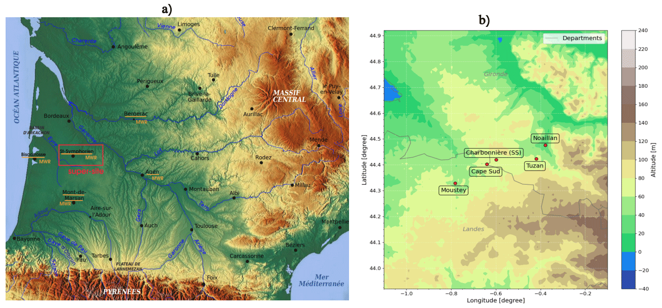
Figure 1 In (a), the orography of the study area of the SOFOG3D field campaign is shown, including the five instrumented sites (Agen, Bergerac, Biscarrosse, Mont-de-Marsan, and Saint-Symphorien), where a microwave radiometer was installed (adapted from https://fr.wikipedia.org/wiki/Grand_Sud-Ouest_français#/media/Fichier:Topographic_map_of_South-West_France_with_main_rivers_and_cities.svg, last access: 18 December 2023). Blue lines indicate the rivers. The cities are indicated in black dots. The most instrumented domain around the supersite is indicated in (a) by the red rectangle. In (b), the orography of a 100×100 km² domain centred on Charbonnière, which includes locations of four of the meteorological stations installed around the supersite and used in this study. Orography data are from the National Aeronautics and Spatial Administration (NASA) shuttle radar topography mission (SRTM) (90 m of resolution).

2.1 Dataset

2.1.1 Surface measurement data

A network of surface weather stations was installed in the study domain of SOFOG3D at the vicinity of Charbonnière to document the spatial variability of fog and surface heterogeneities at the local scale (Fig. 1b). Four weather stations were also deployed around the supersite in a northeast–southwest transect (Fig. 1b). These stations were installed at Moustey, Cape Sud, Tuzan, and Noaillan, almost at the same altitude, and operated continuously with very high temporal resolution (0.1 s time interval) during the period from 18 October 2019 to 31 December 2020. In addition to temperature, pressure, relative humidity sensors, and anemometers, a scatterometer provided the visibility used to estimate fog formation and dissipation times at each station. Temperature data are used to characterise the spatial variability of the radiative cooling, and wind speed and direction are used for the local circulations.

In this study, fog occurrence is defined using the visibility at the supersite based on an algorithm developed by Tardif and Rasmussen (2007). This algorithm consists of dividing visibility time series into 10 min blocks. A fog block means that half of the visibility measurements during a 10 min period are below 1000 m. Blocks are characterised by a positive or negative construct. A positive construct indicates that five consecutive blocks of which the central block is fog and at least two other blocks are also fog blocks. The opposite means a negative construct. Thus, the fog formation time corresponds to the first fog block in the first positive construct encountered. The fog dissipation time corresponds to the last fog block in the last positive construct before either a negative construct or three consecutive non-fog blocks are encountered. This algorithm discards fog events shorter than 1 h.

Météo-France installed in a fallow field near the supersite a sonic anemometers to continuously measure the near-surface (3 m a.g.l.) meteorological conditions (air temperature and relative humidity), the three components of the wind, and pressure at 0.3 m a.g.l.). These instruments provided high-frequency data at 20 Hz. In this study, to document turbulence and thermodynamical processes driving fog phases, we use the sensible heat flux (SHF), turbulence kinetic energy (TKE), and vertical velocity variance (${\mathit{\sigma }}_{\mathrm{w}}^{\mathrm{2}}$). These variables are estimated using eddy covariance methods (Foken et al., 2004; Mauder et al., 2013) calculated every 30 min after quality control of the data. More details on the data can be found in Canut (2020).

2.1.2 Observation of cloud characteristics

For the monitoring of cloud layers, a BASTA cloud radar (Delanoë et al., 2016) was deployed at Charbonnière, and a CL51 ceilometer was deployed at Tuzan (7.4 km northwest of Charbonnière) (Fig. 1b).

BASTA is a 95 GHz cloud radar manufactured by the Laboratoire Atmosphères, Milieux, Observations Spatiales (LATMOS) with an absolute calibration method for frequency-modulated continuous wave (FMCW) cloud radars based on corner reflectors (Toledo et al., 2020). From 7 November 2019 to 12 March 2020, the radar was operated continuously with a vertical pointing mode having three vertical resolutions (12.5, 25, and 100 m). It provided radar reflectivity and Doppler velocity. The lowest mode, which has its first available gate at 37.5 m a.g.l. and 12.5 m of vertical resolution, is used to estimate the cloud top height (CTH), which gives the fog thickness at a time resolution of 30 s. It also provides the level of highest concentration of droplets in the fog layer. The CTH is estimated using a radar reflectivity threshold of −34 dBZ.

The CL51 is manufactured by Vaisala and automatically provided three estimates of cloud base height (CBH), allowing the detection of cloud decks every 30 s with a vertical resolution of 15 m from 10 October 2019 to 2 April 2020. In this study, we use the lowest CBH, which corresponds to the base height of stratus cloud lowering or lifting when fog forms or dissipates, respectively. More information on the data provided by the CL51 can be found in Burnet (2021).

2.1.3 Temperature, liquid water content, and wind profiling

A microwave radiometer Hatpro (MWR) manufactured by Radiometer Physics GmbH (RPG) was installed at the supersite to characterise thermodynamic atmospheric conditions during the field campaign. From 4 December 2019 to 9 May 2020, the MWR operated continuously at the supersite using two spectral bands: the K-band (22.24–31 GHz), which was used for the retrieval of humidity profiles, integrated water vapour (IWV) content, and liquid water path (LWP), and the V-band (51–58 GHz), which was used to retrieve temperature profiles. In order to improve the vertical resolution in the boundary layer, the MWR was set up to scan in 10 elevation angles (5^∘ a.g.l.) every 10 min with a zenith pointing each 1 s. Using neural networks, brightness temperatures measured by the MWR at all elevation angles (the lower elevations angles added to measurements at zenith) are inverted to temperature and humidity variables. More details on this method can be found in Martinet et al. (2022). Comparing temperature and humidity profiles retrieved by the MWR with radiosonde data, Martinet et al. (2022) found that air temperature has cold biases below 0.5 K in absolute value below 2 km but increases up to 1.5 K above 4 km altitude. The low biases in the lowest atmosphere allow a good estimation of the lowest temperature inversion under focus in this study. For each case study, the transition from stable to adiabatic fog is estimated using the static atmospheric stability in the lowest atmosphere computed using the temperature profile. The air temperature profiles are also used to characterise the atmospheric conditions linked to the development of fog at Charbonnière. For the absolute humidity, the maximum dry bias of the MWR is around 1.4 g m⁻³ in the lowest troposphere up to 1.7 km and becomes wet above (0.3 g m⁻³). Martinet et al. (2022) showed that the LWP accuracy has been validated in clear-sky conditions and has shown errors between 1 and 14 g m⁻². These error range are in the scope of those defined in the literature (Crewell and Löhnert, 2003; Marke et al., 2016). The LWP is a key parameter to consider for the microphysical characteristics of fog and is used in the conceptual model. More information regarding the data can be found in Martinet (2021).

The WindCube lidar has become a common instrument used in documenting very low atmospheric phenomena such as turbulence (Liao et al., 2020; Kumer et al., 2016). Dias Neto et al. (2023) demonstrated the usefulness of the wind speed and direction estimated using the WindCube V2. Comparing wind from WindCube V2 with GPS radiosonde, they found low biases of 0.52 m s⁻¹ and 0.37^∘ for the wind speed and direction, respectively. To investigate the dynamics of the atmosphere at the supersite, a WindCube V2 lidar manufactured by Leosphere was deployed by Météo-France during the field campaign to provide the wind measurements at 10 levels ranging from 40 m to 220 m a.g.l. from 1 October 2019 to 10 April 2020. The measurements made at a 1 Hz frequency and a 20 m vertical resolution provided the estimation of turbulence parameters such as the turbulent kinetic energy (TKE). The wind components are estimated every 10 min using a carrier-to-noise ratio (CNR) of at least −23 dB and a total data availability of at least 50 %. Note that the CNR depends on atmospheric turbulence characteristics and relative humidity (Aitken et al., 2012). In the presence of fog or low stratus, the lidar vertical range becomes low. The TKE is computed as the sum of the horizontal variances as in Kumer et al. (2016). Velocity variances are estimated every 30 min using the wind components at the high resolution. It is used in this study to analyse the role of turbulence within the foggy layer to further characterise fog formation, evolution, and dissipation. More details on the WindCube lidar data can be found in Canut (2022).

2.1.4 Fog adiabaticity and reservoir

To further understand fog characteristics, it is essential to focus our analysis on several variables related to the formation, evolution, and dissipation of fog. Fog adiabaticity and reservoir are key metrics driving the life cycle of fog. They are estimated using the fog conceptual model (Toledo et al., 2021) developed at SIRTA. This model is a uni-dimensional model inspired by previous numerical models for stratus clouds (Betts, 1982; Albrecht et al., 1990; Cermak and Bendix, 2011). The basic hypothesis is to consider a well-mixed fog layer and to express the increase in height of the fog liquid water content as a function of the local adiabaticity and the negative of the change in the saturation mixing ratio with height (Γ_ad(T,P)) (Eq. A1). Fog liquid water path is parameterised as a function depending on the equivalent fog adiabaticity (α_eq) and the CTH (Eq. A3). The equivalent fog adiabaticity is used to characterise the buoyancy in low clouds. α_eq varies depending on the in-cloud mixing parameter β and is expressed as ${\mathit{\alpha }}_{\mathrm{eq}}=(\mathrm{1}-\mathit{\beta })$ (Betts, 1982; Cermak and Bendix, 2011). For low-level clouds, such as stratus and stratocumulus, α_eq is between 0.6 and 0.9 (Braun et al., 2018), indicating sufficient buoyancy in the cloud layer with an adiabatic profile. To parameterise this parameter in the fog conceptual model, Toledo et al. (2021) used an inversion of Eq. (A3) to define a fog adiabaticity from closure (${\mathit{\alpha }}_{\mathrm{eq}}^{\mathrm{closure}}$) given as follows:

$$\begin{array}{}\text{(1)}& {\mathit{\alpha }}_{\mathrm{eq}}^{\mathrm{closure}}={\displaystyle \frac{\mathrm{2}\left(\mathrm{LWP}-{\mathrm{LWC}}_{\mathrm{0}}\mathrm{CTH}\right)}{{\mathrm{\Gamma }}_{\mathrm{ad}}(T,P){\mathrm{CTH}}^{\mathrm{2}}}};\end{array}$$

${\mathit{\alpha }}_{\mathrm{eq}}^{\mathrm{closure}}$ depends on the accumulated liquid water content (LWC) at the fog base (LWC₀), the fog thickness (e.g. CTH), the LWP, and the adiabaticity. The adiabaticity lapse rate is a function of air temperature and pressure. Toledo et al. (2021) found that the equivalent fog adiabaticity from closure is negative when the LWP is below 30 g m⁻². They defined the transition phase from stable to adiabatic conditions when the equivalent fog adiabaticity from closure is around 0.5. In the conceptual model, this parameter is estimated only for a CTH below 462.5 m with free cloud above.

The model considers that the fog dissipates when its liquid water path is below a certain threshold depending on the local thermodynamic atmospheric conditions. In case of dissipation by lifting the base height of the fog, Wærsted (2018) found a deficit in LWP in the fog layer. This assertion allows for defining a minimum amount of LWP necessary to maintain the horizontal visibility at surface lower or equal to 1000 m, defined as the critical liquid water path (CLWP). Thus, based on Eq. (A3), the CLWP can be expressed in Eq. (2) considering a critical liquid water content at surface (LWC_c).

$$\begin{array}{}\text{(2)}& \mathrm{CLWP}={\displaystyle \frac{\mathrm{1}}{\mathrm{2}}}{\mathit{\alpha }}_{\mathrm{eq}}{\mathrm{\Gamma }}_{\mathrm{ad}}(T,P){\mathrm{CTH}}^{\mathrm{2}}+{\mathrm{LWC}}_{\mathrm{c}}\mathrm{CTH}\end{array}$$

Theoretically, the LWC_c corresponds to the LWC that would cause a 1000 m visibility. It is estimated from the parameterisation of Gultepe et al. (2006) based on the horizontal visibility at surface.

Considering that adiabatic fog exists because the liquid water path in its thickness is strictly greater than or equal to its CLWP (Toledo et al., 2021), it is possible to define an associated quantity named the fog reservoir of liquid water path (RLWP). The RLWP is defined as the difference between fog current liquid water path and the critical value as follows:

$$\begin{array}{}\text{(3)}& \begin{array}{rl}\mathrm{RLWP}& =\mathrm{LWP}-\mathrm{CLWP}=\mathrm{LWP}-{\displaystyle \frac{\mathrm{1}}{\mathrm{2}}}{\mathit{\alpha }}_{\mathrm{eq}}{\mathrm{\Gamma }}_{\mathrm{ad}}(T,P){\mathrm{CTH}}^{\mathrm{2}}\\ & -{\mathrm{LWC}}_{\mathrm{c}}\mathrm{CTH}.\end{array}\end{array}$$

The RLWP depends on the LWCc (Eq. A4), the adiabaticity, and fog thickness. The calculation of RLWP can be used to anticipate the dissipation or thickening of the fog in the coming minutes or hours. Based on 20 fog cases at SIRTA, Toledo Bittner (2021) found that for a RLWP > 30 g m⁻² in a given time instant, fog does not dissipate within the following 30 min. He also showed that the RLWP trend decreases before fog dissipation time and increases when fog is persisting. This behaviour motivates the analysis of the RLWP trend in this study to improve the characterisation of the different fog phases.

The number of fog events observed during the SOFOG3D field campaign is not sufficient to calibrate the fog conceptual model in southeastern France as it was in SIRTA (Toledo et al., 2021). In this study, we use the model with its parameterisation at SIRTA to further characterise the different phases observed in the lifetime of fog based on identified case studies. The model is performed when the visibility is lower than 1000 m. ${\mathit{\alpha }}_{\mathrm{eq}}^{\mathrm{closure}}$ is used to characterise the fog transition from stable phase to adiabatic phase. The RLWP gives an estimation of the excess or deficit of liquid water of the fog that enables the fog layer to remain at surface or dissipate. It can be used as a diagnostic of how likely the fog will persist in the coming minutes or hours (i.e. as a nowcasting tool for fog dissipation time). More details on the fog conceptual model are given in Appendix A and can be found in Toledo Bittner (2021).

2.2 Case studies and methodological approach

For the whole SOFOG3D campaign, based on the fog defined criteria described in Sect. 2.2.1, 31 fog events are identified during the 31 October 2019–26 March 2020 period. For each one, a visual inspection of the time–height cross-section of the radar reflectivity from BASTA cloud radar and the cloud base height from the ceilometer was carried out. We selected the four most developed fog episodes, namely case studies 1 (IOP 5), 2 (IOP 6), 3 (IOP 11), and 4 (IOP 14).

As in Toledo et al. (2021) (their Fig. 3), Fig. 2 shows the equivalent adiabaticity by closure versus LWP and CTH for the four fog cases studied. It indicates that ${\mathit{\alpha }}_{\mathrm{eq}}^{\mathrm{closure}}$ reaches 0.5 when LWP > 20 g m⁻² and the CTH > 150 m, which should be the conditions favourable for the fog to become optically opaque to the infrared radiation. At the supersite, the LWP observed during that transition is lower than the threshold at SIRTA (LWP > 30 g m⁻²) (Wærsted et al., 2017; Toledo et al., 2021). However, there is a consistency between both sites on the computation of the equivalent adiabaticity by closure. This legitimises the choice of the four cases and motivates the use of the ${\mathit{\alpha }}_{\mathrm{eq}}^{\mathrm{closure}}$ in this study to define the transition phase between stable and adiabatic fog.

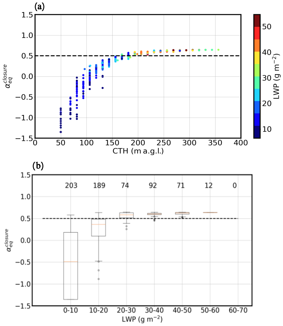
Figure 2 (a) Scatter plot of the equivalent adiabaticity by closure versus the CTH and LWP (colored circles) at the supersite. (b) Boxplot of the equivalent adiabaticity by closure versus the different LWP ranges from the MWR. In (b), numbers at the top of the figure indicate total values included in each boxplot and computed between 2 h before and after the fog. The horizontal dashed line indicates the threshold of the equivalent adiabaticity from closure, defining the transition from stable to adiabatic fog.

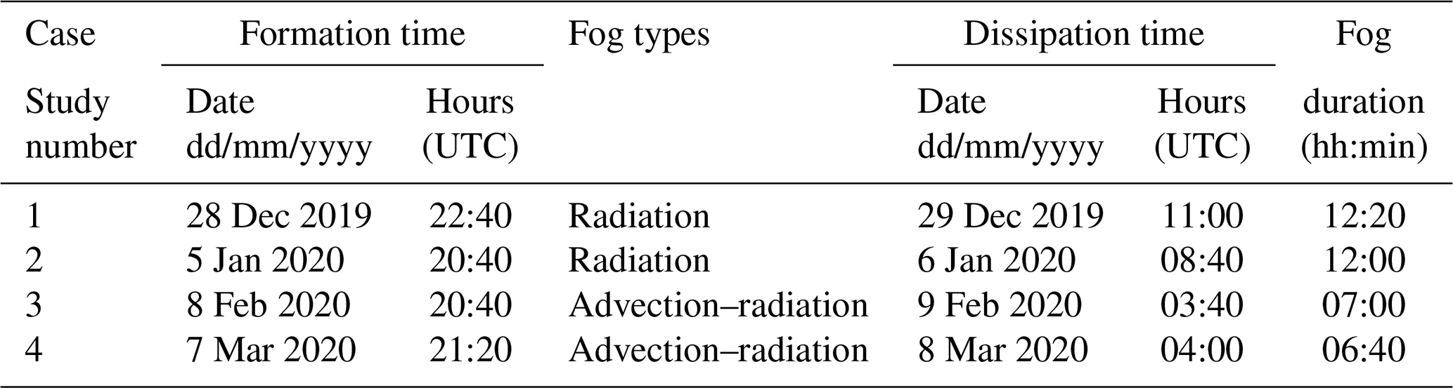
For the selected case studies, Table 1 contains the fog formation and dissipation times, fog formation types, and fog duration at the supersite. For all selected fog events, the formation time of fog is observed between 20:40 and 22:40 UTC, while the dissipation time varies from night-time to daytime. These selected fog events are triggered by radiation (two cases) or advection–radiation (two cases) processes.

Table 1 Case study number, fog onset time, type of fog formation, fog dissipation time, fog duration, and type of fog dissipation for the four documented case studies. Time is in UTC. Dates are in the format dd/mm/yyyy.

For each selected case study, temperature profiles from the MWR, radar reflectivity profiles from the BASTA cloud radar, and the equivalent fog adiabaticity derived from the conceptual model are used to define the four fog phases characterising the fog evolution: fog pre-onset, stable fog, adiabatic fog, and fog dissipation. Note that an important time of the fog life cycle is the transition time between stable and adiabatic fog. Each fog phase is defined as follows.

1. Fog pre-onset corresponds to the 2 h preceding fog onset associated with cloud-free conditions.

2. In the four case studies, the stable phase starts at fog onset. It is characterised by a stable temperature profile in the lowest 100 m of the atmosphere.

3. The transition time separating the stable and adiabatic phases can be defined differently depending on the meteorological variables considered. Price (2011) defined this transition time as the time when the air temperature becomes constant in the fog lowest layer (1.5–50 m a.g.l.). Toledo et al. (2021) found that the transition is observed when the equivalent fog adiabaticity by closure is increasing between 0 and 0.5. In this study, for a better definition of this period, we take into account the static stability given by the hourly profiles of mean air temperature from the MWR, the fog geometry (CTH) from the cloud radar, and the ${\mathit{\alpha }}_{\mathrm{eq}}^{\mathrm{closure}}$ from the conceptual model. Indeed, the transition period is defined as the time when the temperature profile becomes unstable or neutral in the 0–75 m a.g.l. layer, while the fog CTH increases with time, and ${\mathit{\alpha }}_{\mathrm{eq}}^{\mathrm{closure}}$ increases from 0 to about 0.5. Note that the thickening of the fog is associated with the elevation of the level of the maximum radar reflectivity. The transition phase starts when ${\mathit{\alpha }}_{\mathrm{eq}}^{\mathrm{closure}}<\mathrm{0.5}$, the CTH suddenly increases more than 25 m in 5 min under a stable or neutral layer. This phase ends when ${\mathit{\alpha }}_{\mathrm{eq}}^{\mathrm{closure}}$ reaches 0.5 and the fog layer becomes neutral or unstable.

4. Fog adiabatic phase is characterised by ${\mathit{\alpha }}_{\mathrm{eq}}^{\mathrm{closure}}$ around 0.5, a neutral or unstable temperature profile, and a radar reflectivity that increases with increasing altitude and peaks a few 10ths of a metre below cloud top.

5. The fog dissipation phase is defined as being the period of 30 min before and after dissipation time (when horizontal visibility becomes greater than 1 km). Since the fog dissipation time does not appear abruptly, as it is also driven by thermodynamical processes, we consider this time range to further document them.

Based on these fog phase definitions, in the following we describe the four case studies. For each fog event, we document the processes involved in the evolution of fog in each of these phases using the fog conceptual model and the instrumental synergy in order to identify the main processes driving the fog life cycle.

3 Fog formation, evolution, and dissipation processes

3.1 Radiation fog case studies

3.1.1 Case study 1 (IOP 5) analysis

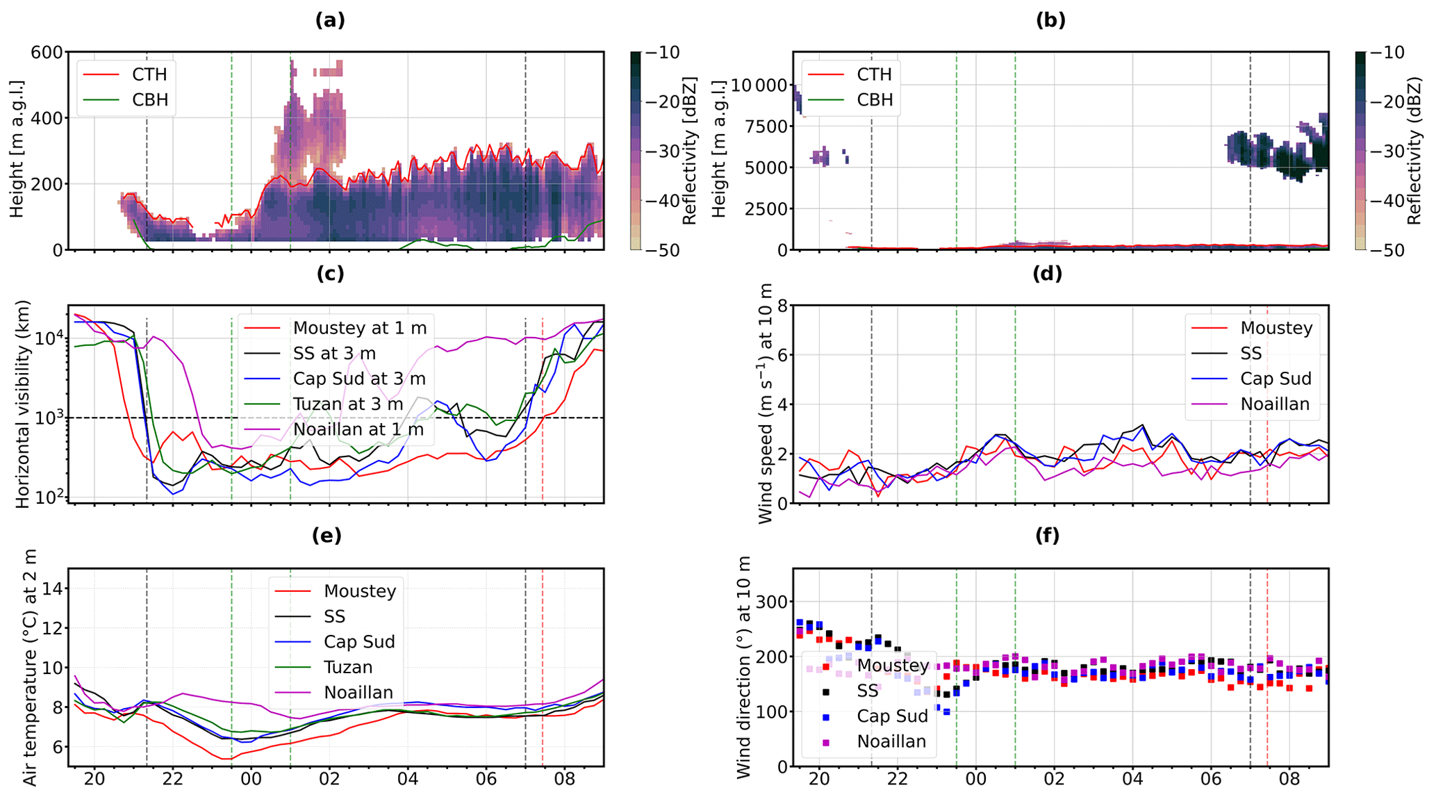
Figure 3a and b indicate the time cross-sections of the radar reflectivity estimated from BASTA cloud radar during case study 1 on 28–29 December 2019 up to 600 and 12 000 m, respectively. They show a clear sky before the fog formation time at 22:40 UTC on 28 December 2019. During fog evolution, cloud-free conditions are observed above the fog top height until 09:00 UTC when sparse thin high-altitude clouds occur above the cloud radar. Figure 3c presents a quasi-homogeneous fog formation time between the three sites and a heterogeneous dissipation time. At Charbonnière, fog dissipated at 11:00 UTC on 29 December 2019 and 2 h earlier at Noaillan. At all sites, low temperatures below 4 ^∘C (Fig. 3e) are observed during the fog period. Near the surface, light winds (<1 m s⁻¹) are recorded at all sites from fog pre-onset to fog stable–adiabatic transition times (Fig. 3d and f).

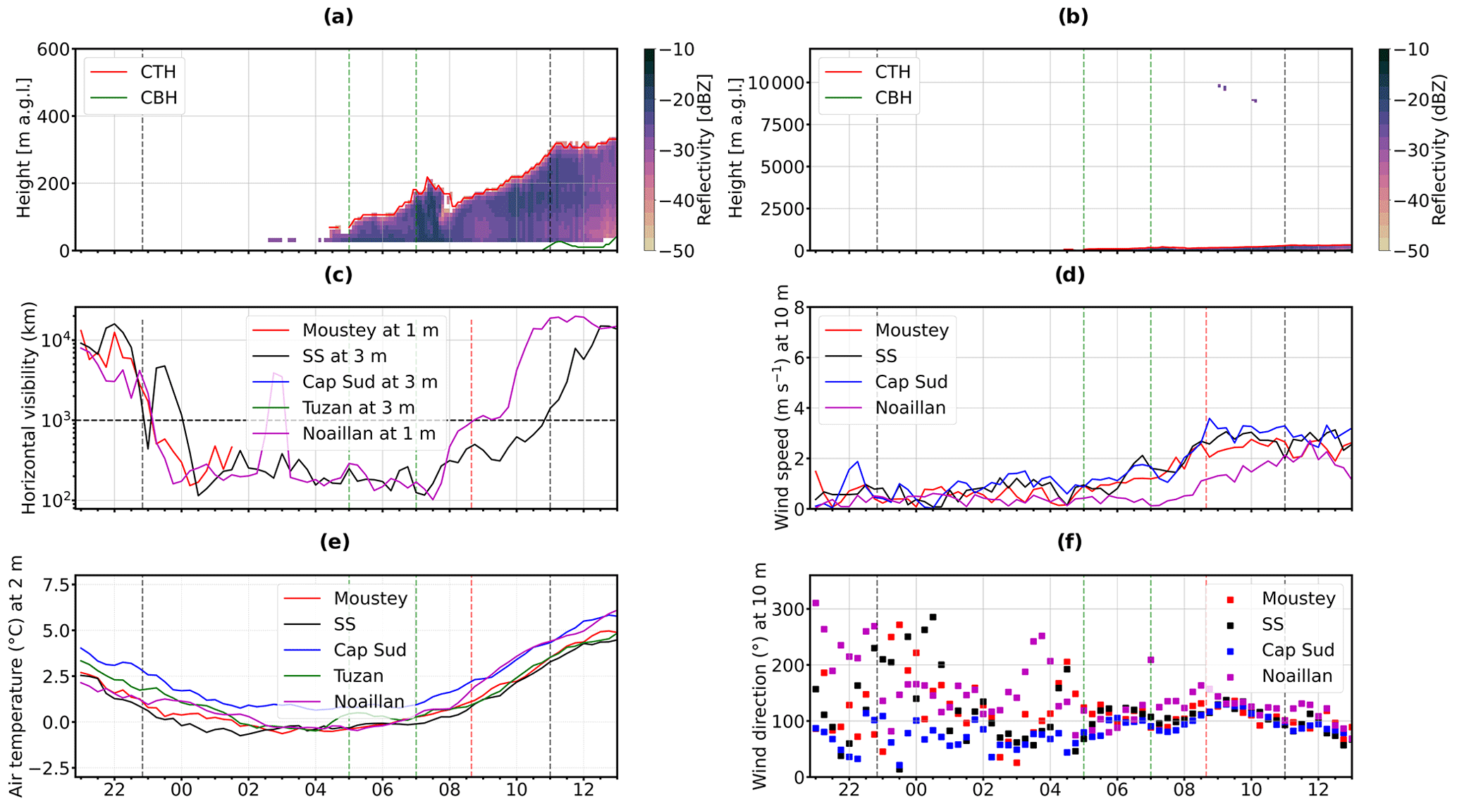
Figure 3 In (a, b) a time–height cross-section is given from the surface up to 600 and 12 000 m, respectively, of the radar reflectivity from BASTA (shaded), the time evolution of the cloud top height from BASTA (red line), and the cloud base height from the ceilometer (CL51) (green line). Time evolution of (c) surface visibility, (d) 10 m wind speed, (e) 2 m air temperature, and (f) 10 m wind direction observed on the 28–29 December 2019 (case study 1, IOP 5) at the five meteorological stations (red, black, blue, green, and pink lines for Moustey (1 m a.g.l.), Charbonnière (3 m a.g.l.), Cape Sud (3 m a.g.l.), Tuzan (3 m a.g.l.), and Noaillan (1 m a.g.l.), respectively) deployed around the supersite. Note that wind was not collected at Tuzan. In (c), the visibility measured at Moustey was interrupted by technical issues. Vertical dashed black lines indicate fog formation (left) and dissipation (right) times. Dashed green lines show the transition time from stable fog to adiabatic fog (fog mature phase). The dashed red line indicates the sunrise.

The fog pre-onset is marked by a double stratification of the atmospheric boundary layer with a thin inversion from the surface up to 100 m and deep and strong inversion (around 8 ^∘C km⁻¹) above (Fig. 4a). Atmospheric conditions are dominated by an easterly wind that reaches 5 m s⁻¹ above 100 m a.g.l., which is possibly due to a low-level jet (Fig. 4d). The mean cooling rate near the surface is −0.9 ^∘C h⁻¹. The strong decrease in temperature is associated with a negative SHF (−0.23 W m⁻²) (Fig. 4h), near-surface low wind (0.61 m s⁻¹) (Fig. 3d and f), and low turbulence (TKE = 0.11 m² s⁻² and ${\mathit{\sigma }}_{\mathrm{w}}^{\mathrm{2}}=\mathrm{0.002}$ m² s⁻²). These conditions lead to thermally stable atmospheric conditions that are favourable for radiation fog formation (Table 1).

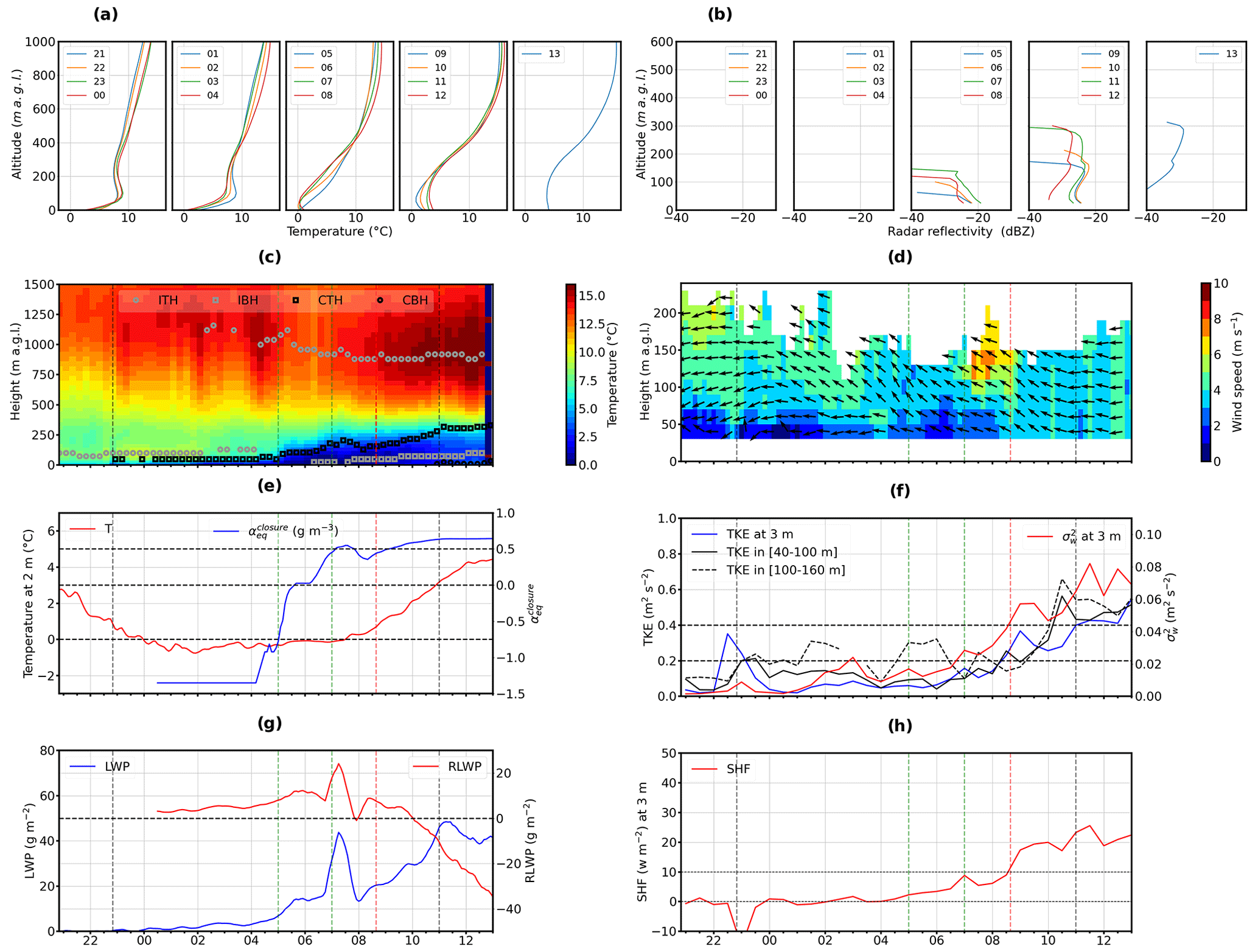
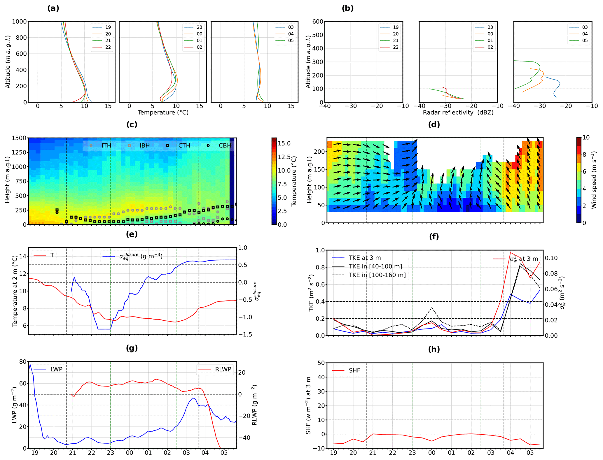
Figure 4 Evolution of fog macrophysical characteristics observed on the 28–29 December 2019 (case study 1, IOP 5) at Charbonnière. Panels (a) and (b) show vertical profiles of air temperature from the Hatpro microwave radiometer (MWR) and radar reflectivity from BASTA radar, respectively. Panel (c) shows a time–height cross-section of air temperature from the MWR (shaded), time evolution of inversion top height (ITH) (open grey squares), inversion base height (IBH) (open grey squares), and cloud top height (CTH) from the cloud radar (open black squares) and the cloud base height (CBH) from the ceilometer (open black circles). Panel (d) shows wind speed (shaded) and direction (arrows) from the WindCube. Arrows in (d) indicate only the direction of the horizontal flow. (e) Time evolution of air temperature at 3 m a.g.l. from the meteorological station (red line) and equivalent adiabaticity of closure from the fog conceptual model (blue line). (f) The mean of the turbulent kinetic energy (TKE) in the layer 40–220 m (solid black line) and 100–160 m a.g.l. (dashed black line) from the WindCube (black line) and the TKE (blue line) and vertical velocity variance (red line) at 3 m a.g.l. from the flux station at Charbonnière. (g) The LWP estimate from the MWR (blue line) and the RLWP from the fog conceptual model (red line). (h) Sensible heat flux (SHF) (red) from the flux station. Vertical dashed black lines indicate fog formation and dissipation times. Dashed green lines indicate the transition period (fog mature phase) from stable to adiabatic fog. The dashed red line indicates sunrise.

The fog stable phase lasts around 6 h (22:50–05:00 UTC) and is characterised on average by a very low negative near-surface cooling rate (−0.18 ^∘C h⁻¹), an almost zero SHF, an easterly light wind (0.78 m s⁻¹), low turbulence (TKE = 0.07 m² s⁻², ${\mathit{\sigma }}_{\mathrm{w}}^{\mathrm{2}}=\mathrm{0.01}$ m² s⁻²), negative ${\mathit{\alpha }}_{\mathrm{eq}}^{\mathrm{closure}}$ (−1.3) (Fig. 4e), low LWP (2.18 g m⁻²) (Fig. 4g), slight increase in time of the fog thickness up to 50 m, and relatively stable temperature inversion height. These characteristics maintain the thermally stable fog with a horizontal visibility of 736 m on average.

The transition time from stable to adiabatic fog is observed between 05:00 and 07:00 UTC (2 h duration) and associated with the lowest visibility (198 m), a transition in the vertical profiles of air temperature (Fig. 4a) from stable at 05:00 UTC to unstable at 06:00 UTC in the fog layer, a deepening of the cold layer, an increase in the mean SHF reaching 44 and around 10 W m⁻² at the phase end (Fig. 4h), and an increase in the turbulence (TKE up to 0.15 m² s⁻² and ${\mathit{\sigma }}_{\mathrm{w}}^{\mathrm{2}}$ up to 0.04 m² s⁻²) generated by the strengthening of the wind speed (1.14 m s⁻¹) and its shift in direction from east to southeast. From 05:00 to 06:00 UTC, the coldest temperature shifts from the surface up to 50 m a.g.l., and the vertical profile of radar reflectivity increases with height, indicating a vertical development of fog (Fig. 4b) generated by turbulence processes. At the end of this phase, ${\mathit{\alpha }}_{\mathrm{eq}}^{\mathrm{closure}}$ reaches 0.5, which is consistent with the threshold obtained at the SIRTA site by Toledo et al. (2021). The ${\mathit{\sigma }}_{\mathrm{w}}^{\mathrm{2}}$ values observed are higher than the threshold fixed by Price (2019) for a thermally stable surface layer. The LWP (28 g m⁻²) and RLWP (+15 g m⁻²) peak at the end of the transition phase consistently with a decrease in visibility. Due to the simultaneous increase in SHF, TKE, and ${\mathit{\sigma }}_{\mathrm{w}}^{\mathrm{2}}$, the transition phase is driven by both thermal and mechanical turbulence.

The fog adiabatic phase is observed between 07:00 and 11:00 UTC (4 h duration) at the supersite and characterised by a vertical development of fog up to 187.5 m (Fig. 4b) and the arrival of sparse high clouds (Fig. 3a and b) associated with the lowering of the temperature inversion top height above the fog top (Fig. 4c). Note that these clouds have no effect on the radiative cooling at the top height of the fog. The fog layer becomes warmer (+0.77 ^∘C h⁻¹ on average), and its LWP and RLWP reach 26.16 and +6.38 g m⁻², respectively. The turbulence gradually increases in the fog layer (Fig. 4f) (TKE = 0.23 m² s⁻²) due to an increase in the horizontal wind speed (2.4 m s⁻¹) combined with an increase in the vertical shear and the wind shift from southeasterly to easterly (Fig. 4d). In the same way, ${\mathit{\sigma }}_{\mathrm{w}}^{\mathrm{2}}$ increases to 0.04 m² s⁻² and is driven both by the vertical wind shear and the increase in SHF (12.9 W m⁻²) (Fig. 4h). For this case study, the moderate mechanical and thermal turbulence causes the vertical mixing in the fog layer, which slightly increases the surface horizontal visibility (370 m) and fog top height (185 m).

At the supersite, in the absence of any cloud above the fog layer, the fog dissipates after sunrise. It is marked by a continued increase in SHF (Fig. 4h) due to solar radiation (daytime atmospheric convection), negative RLWP (−11.39 g m⁻²), an increase in CTH (290 m), LWP (maximum of 43.34 g m⁻²), stable ${\mathit{\alpha }}_{\mathrm{eq}}^{\mathrm{closure}}$ around 0.63, and more thermal turbulence (${\mathit{\sigma }}_{\mathrm{w}}^{\mathrm{2}}=\mathrm{0.06}$ m² s⁻²) allowing more vertical mixing. Based on the RLWP, the fog conceptual model would predict a deficit of liquid water in the fog layer 1 h before the lifting of its base height (Fig. 4g). The fog dissipation phase is induced by the increase in the vertical mixing generated by the thermal (solar heating) and mechanical turbulence associated with TKE values larger than 0.4 m² s⁻² (Fig. 4f).

In summary, for this radiative fog event, the fog conceptual model is consistent with the in situ measurements of turbulence on the timing of the different fog phases. It has provided additional elements for understanding the different phases of the fog life cycle.

3.1.2 Case study 2 (IOP 6) analysis

As in case study 1, case study 2 is a radiation fog that forms under clear skies a few hours after sunset (Fig. 5a and b) under a double stratification of the low atmosphere (Fig. 6a), southerly very low near-surface wind speed (0.2 m s⁻¹), low TKE (0.06 m² s⁻²), and negative surface SHF. The fog lasts 12 h and completely dissipates around 08:40 UTC on 6 January 2020 at the supersite (see Table 1) and at 04:30 UTC at Noaillan, revealing more spatial variability than in case study 1.

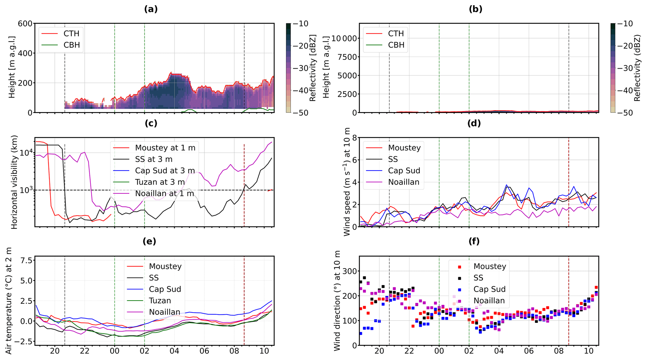
Figure 5 The same as Fig. 3 but for 5–6 January 2020 (case study 2, IOP 6). In (c) only Charbonnière and Noaillan have valid data. In (c) the visibility measured at Moustey, Tuzan, and Cape Sud was interrupted by technical issues.

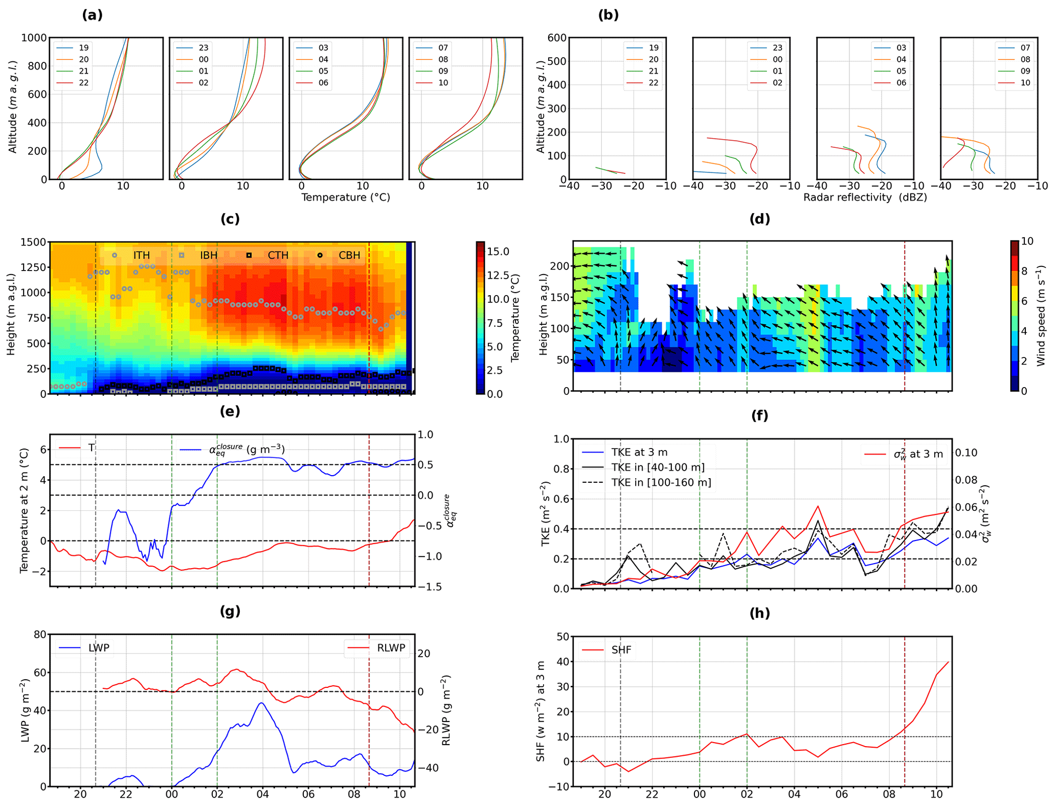
Figure 6 The same as Fig. 4 but for 5–6 January 2020 (case study 2, IOP 6). The vertical dashed red line indicates the sunrise.

The fog stable phase lasts 3 h 20 min (20:40 to 00:00 UTC), half the time of case study 1, with fog characteristics similar to those of case study 1. A 2 h fog transition phase is observed from 00:00 to 02:00 UTC, (2 h duration as for IOP 5) at the supersite (Fig. 6a and b) and characterised by positive SHF (7.76 W m⁻²) and larger values of TKE (0.23 m² s⁻¹) allowing vertical mixing and transition towards adiabatic fog. A significantly longer fog adiabatic phase is observed from 02:00 to 08:40 UTC (twice longer than in IOP 5). The first period from 02:00 to 05:00 UTC is characterised by continued positive SHF (10 W m⁻²) (Fig. 6h) and significant turbulence (TKE > 0.2 m² s⁻² and ${\mathit{\sigma }}_{\mathrm{w}}^{\mathrm{2}}>\mathrm{0.02}$ m² s⁻²) (Fig. 6f) leading to a deeper fog with relatively high LWP (42 g m⁻²) and a positive RLWP until 04:30 UTC (Fig. 6g). The second period from 05:00 to 08:40 UTC is characterised by continued positive SHF an significant ${\mathit{\sigma }}_{\mathrm{w}}^{\mathrm{2}}$ (>0.02 m² s⁻²), while the TKE decreases (<0.2 m² s⁻²) associated with the decrease in wind speed in the fog layer. A sharp decrease in LWP, with a reduction in fog top height, leads to RLWP oscillating around 0 g m⁻², and the horizontal visibility increases and then decreases again. During this period, the sharp decrease in LWP (<20 g m⁻²) results in a fog layer that is not very resilient to the significant turbulence, as shown by the very low RLWP values and rapidly changing horizontal visibility (Fig. 5c). The decrease in LWP could be driven by production of drizzle, as reported through droplets freezing on the tethered balloon. Fog dissipation occurred after sunrise (08:40 UTC, under positive SHF (14 W m⁻²) driven by the turbulence associated with mechanical and thermal processes (mean TKE ∼ 0.28 m² s⁻² and ${\mathit{\sigma }}_{\mathrm{w}}^{\mathrm{2}}\sim \mathrm{0.048}$ m² s⁻²).

3.2 Radiation–advection fog case studies

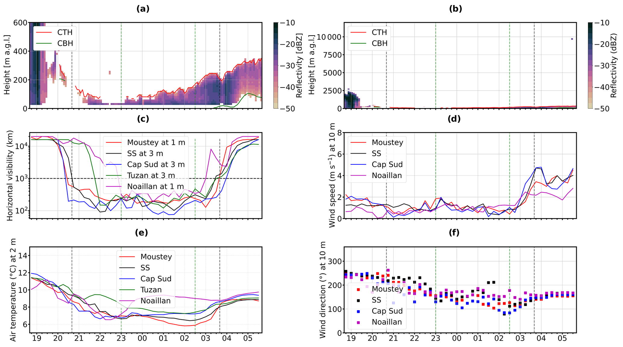
Case studies 3 and 4 correspond to two fog cases that form after sunset (near 21:00 UTC) in a moist westerly flow, with an initial condensation about 100 m a.g.l. (ultra-low stratus or elevated fog) followed by a rapid subsidence of the cloud layer to the ground (see Figs. 7 and 9, respectively). West–east gradients are observed in terms of temperature and fog formation time, combined with a weak temperature inversion at the time of fog formation, justifying the classification of fog formation by advection–radiation processes (Ryznar, 1977).

Figure 7 The same as Fig. 3 but for 8–9 February 2020 (case study 3, IOP 11).

3.2.1 Case study 3 (IOP 11) analysis

In spite of different formation conditions for case study 3, compared to case 1 and 2, the stable fog phase of this case is characterised by fog conditions that are similar to those of case 1 and 2 (Fig. 8): slightly negative SHF, low turbulence (TKE = 0.03 m² s⁻²), and low LWP (<10 g m⁻²). Case study 3 differs from the previous case studies as it has a longer duration for the stable-to-adiabatic fog transition (3 h 30 min duration), during which SHF remains slightly negative; TKE remains mostly below 0.03 m² s⁻²; and CTH, LWP, and ${\mathit{\alpha }}_{\mathrm{eq}}^{\mathrm{closure}}$ increase progressively, while RLWP remains relatively stable (5–10 g m⁻²). In case study 3, the very short fog adiabatic phase (1 h) is characterised by increasing vertical wind shear near fog top height (Fig. 8d) that generates dynamical instability driving the vertical mixing, reducing the temperature inversion above fog top (Fig. 8c) and promoting vertical development of the fog layer. The rapid increase in CTH is not sufficiently compensated for by the increase in LWP, leading to a decrease in RLWP (Fig. 8g) and subsequent increase in near-surface visibility and dissipation of the fog. Increasing wind aloft brings warm drier air over the top of the fog that then mixes into it (TKE = 0.33 m² s⁻² and ${\mathit{\sigma }}_{\mathrm{w}}^{\mathrm{2}}=\mathrm{0.07}$ m² s⁻²), evaporating fog droplets, reducing the RLWP to negative values, and causing the fog to lift into low stratus. The fog dissipation phase is thus driven by the advection of warm air at the supersite (Fig. 7e).

Figure 8 The same as Fig. 4 but for 8–9 February 2020 (case study 3, IOP 11).

Figure 9 The same as Fig. 3 but for 7–8 March 2020 (case study 4, IOP 14).

3.2.2 Case study 4 (IOP 14) analysis

As in case study 3, fog case study 4 starts with a very low stratus fog and subsidence of the cloud layer resulting in a fog. The fog layer is perturbed by the advection from the northwest (captured in Meteosat Second image, not shown) around 00:30 UTC of another stratus with a base height above the fog top height. From 04:00 UTC, the fog becomes intermittent with a first dissipation observed at that time and a definitive dissipation around 07:00 UTC.

The 2 h long fog stable phase is also characterised by a cooling rate near −1 ^∘C h⁻¹, slightly negative SHF and low turbulence (TKE < 0.1 m² s⁻²). The relatively short transition from stable to adiabatic fog (<1 h 30 min) is characterised by an increase in mechanically driven turbulence (wind shear, Fig. 10d) with a southerly wind that likely brings additional moisture, leading to a rapid increase in both CTH and LWP (near 40 g m⁻²).

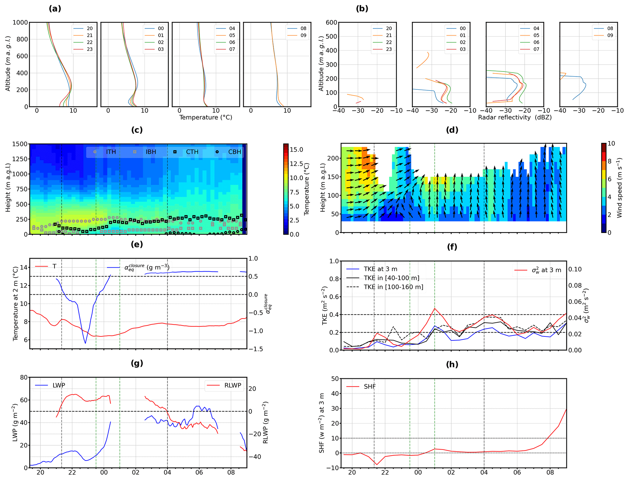
Figure 10 The same as Fig. 4 but for 7–8 March 2020 (case study 4, IOP 14). The LWP, RLWP, and ${\mathit{\alpha }}_{\mathrm{eq}}^{\mathrm{closure}}$ are disrupted between 00:30 and 02:30 UTC because the LWP estimated by the MWR takes into account the liquid water in the advected stratus.

The fog adiabatic phase is observed from 00:20 to 04:00 UTC (3 h 40 min duration) followed by a temporary dissipation of the fog from 04:00 to 05:30 UTC and a definitive fog dissipation at 07:00 UTC. This adiabatic phase is characterised by a 250–300 m deep fog with 40–50 g m⁻² LWP. The mechanically driven TKE ranges between 0.2–0.4 m⁻² s⁻² (Fig. 10f), which confirms the turbulence that a relatively deep fog layer can withstand. The evolution of RLWP to negative values after 04:00 UTC (Fig. 10g) shows that the conceptual model captures the transition from an adiabatic fog with low near-surface visibility (<300 m) to one with horizontal visibility at or above 1000 m (Fig. 9c). The definitive dissipation is not associated with increasing turbulence but rather with the presence of middle-altitude clouds that likely reduce significantly the fog top radiative cooling, as precisely characterised by Waersted et al. (2017), and hence liquid water content production. Indeed, Fig. 10g reveals a significant LWP reduction after 06:30 UTC that explains the definitive dissipation of the fog before sunrise.

4 Discussion

Figure 11 shows the mean vertical profiles of air temperature derived from the MWR and radar reflectivity measured by the cloud radar for each fog phase and each case study. It highlights the thermal and microphysical characteristics of fog phases and differences in atmospheric conditions between fog categories: radiation and radiation–advection fogs.

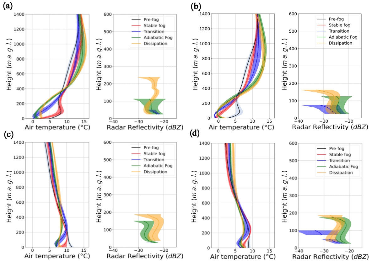
Figure 11 Vertical profiles of air temperature and radar reflectivity put together for each fog case study: (a) case 1, (b) case 2, (c) case 3, and (d) case 4. Lines and shaded areas indicate the mean and standard deviation of air temperature and radar reflectivity during each fog phase.

For radiation fog case studies (1 and 2), fog develops below the dry, warm, and cloud-free stable atmospheric boundary layer (Figs. 4c and 6c). Atmospheric conditions preceding (2 h before) fog formation are dominated by a strong and thick temperature inversion (more than 14 ^∘C and 1000 m), which is associated with anticyclonic conditions over Europe favouring easterly wind and clear sky across the studied area. These atmospheric conditions allow a strong surface radiative cooling, negative heat fluxes, and cooling of near-surface air at a rate of −0.9 and −0.7 ^∘C h⁻¹ for case study 1 and 2, respectively. This cooling is associated with low turbulence indicated by low values of TKE (0.18 m² s⁻² in case 1 and 0.06 m² s⁻² in case 2) and near-surface vertical velocity variance (${\mathit{\sigma }}_{\mathrm{w}}^{\mathrm{2}}<\mathrm{0.003}$ m² s⁻²) that reinforce the surface thermally stable boundary layer (Fig. 11a and b), favouring the triggering of radiation fog. These results are consistent with the definition of radiation fog proposed by Price (2019).

In advection–radiation fog case studies (3 and 4), 2 h before fog formation a westerly sea breeze is present, transporting mild wet air from the ocean. Surface heat fluxes are negative, favouring cooling of the near-surface air (−1 ^∘C h⁻¹ in case study 3 and −0.5 ^∘C h⁻¹ in case study 4), and turbulent mixing is low (TKE < 0.06 m² s⁻²). An east–west gradient of formation and dissipation is observed in line with the westerly synoptic advection of Atlantic inflow. Fog forms earlier in the west and dissipates later in the east. The combination of advection and radiative cooling favours stratus fog formation at about 150 m a.g.l. followed by a rapid (less than 30 min) lowering of its base height to the surface, triggering the onset of the fog in an unstable (case 3) and neutral (case 4) surface atmospheric boundary layers (Fig. 11c and d).

The stable fog phase is characterised by a stable temperature profile and radar reflectivity that is at its maximum near the surface and decreases with height (see Fig. 11). The fog remains shallow (less than 100 m), with a low LWP ranging less than 12 g m⁻² proportional to fog depth (Table 2). The equivalent fog adiabaticity by closure parameter (${\mathit{\alpha }}_{\mathrm{eq}}^{\mathrm{closure}}$) is typically negative during the stable phase, indicating that the fog is not in an adiabatic phase. The near-surface temperature decreases very moderately (−0.2 ^∘C h⁻¹) in cases 1 and 2, while the air keeps cooling at about −1 ^∘C h⁻¹ in cases 3 and 4. For the four cases, surface heat fluxes are slightly negative (−3 to 0 W m⁻²) and turbulence remains low (TKE at about 0.1 m² s⁻² and ${\mathit{\sigma }}_{\mathrm{w}}^{\mathrm{2}}$ at 0.01 m² s⁻²). This phase is characterised by very low LWPs (1–2 g m⁻² for radiation fog and 6–11 g m⁻² for advection–radiation fog). For the radiation fog cases, the stable phase lasts around 6 and 4 h, respectively, while for advection–radiation cases, it lasts around 2 h. This is consistent with the strength of the surface inversion of each category of fog, as shown in Fig. 11. These macrophysical characteristics of the fog stable phase are consistent with those found by Toledo et al. (2021).

Table 2 Summary of fog features at the supersite during the five defined phases of its evolution for each case study. The formation and dissipation times are estimated using the visibility (m) from a scatterometer. The cooling rate ($\mathrm{d}T/\mathrm{d}t$), wind speed (WS), and wind direction (WD) are derived from the meteorological station. Sensible heat flux (SHF), turbulent kinetic energy (TKE), and the vertical velocity variance (${\mathit{\sigma }}_{\mathrm{w}}^{\mathrm{2}}$) at 3 m a.g.l. are derived from the flux station. The liquid water path (LWP) is estimated from the MWR. The fog reservoir of the liquid water path (RLWP) and the equivalent adiabaticity of closure ${\mathit{\alpha }}_{\mathrm{eq}}^{\mathrm{closure}}$ parameter are computed by the conceptual model. Cloud top height (CTH) and middle and high cloud base and cloud top heights are derived from the radar reflectivity from the BASTA cloud radar. Dashes indicate that the variables are not measurable or calculable.

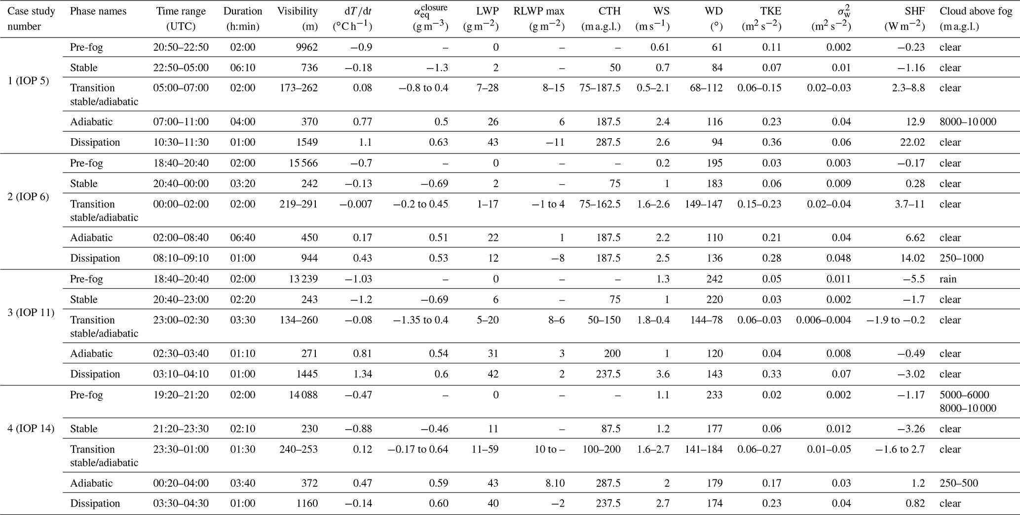
The transition from stable to adiabatic phases is a key period in the fog life cycle. This period is well characterised using the macrophysical parameters of the conceptual model, namely the equivalent fog adiabaticity by closure (${\mathit{\alpha }}_{\mathrm{eq}}^{\mathrm{closure}}$) parameter of the fog, the fog geometry (CTH), and fog LWP. During the transition from stable to adiabatic phases, these three parameters increase significantly (see Table 2). In particular, ${\mathit{\alpha }}_{\mathrm{eq}}^{\mathrm{closure}}$ evolves progressively from negative values towards +0.5 (Toledo et al., 2021). The transition phase lasts from 1 h 30 min to 3 h 30 min; however, its timing of occurrence is quite variable (case 1 at 05:00–07:00 UTC, case 2 at 00:00–02:00 UTC, case 3 at 23:00–02:30 UTC, and case 4 at 23:30–01:00 UTC). During this phase, a change is observed in static stability from stable profiles to neutral adiabatic profiles (Fig. 11), while the radar reflectivity profile presents maximum values near the ground that decrease with height (Fig. 11). In cases 1, 2, and 4, the transition phase is characterised by an increase in turbulence that can explain the decrease in thermal stability of the fog layer, either shown in the vertical velocity variance (${\mathit{\sigma }}_{\mathrm{w}}^{\mathrm{2}}\ge \mathrm{0.02}$ m² s⁻²) associated with positive surface heat fluxes (cases 1 and 2) or TKE exceeding 0.3 m² s⁻² (cases 2 and 4). In all the cases, the fog LWP increases significantly, which allows a more efficient radiative cooling of the fog layer, hence contributing to the destabilisation of the fog layer. In case 3, the transition phase is not marked by a significant increase in turbulence. The transition is more progressive than in the other case studies, with gradual increases in CTH, LWP, and ${\mathit{\alpha }}_{\mathrm{eq}}^{\mathrm{closure}}$ during this long phase (3 h 30 min duration).

According to temperature vertical profiles from the MWR, at the end of the transition time from stable to adiabatic fog, the temperature profile becomes neutral or slightly unstable. This is consistent with the definition of the transition given by Price (2011). We also find that it is during this period that the fog reaches its maximum value of RLWP, showing that the LWP increases beyond the critical liquid water path value, which gives information on the persistence of fog.

For radiation fog case studies, the adiabatic phase lasts 4 h and 6 h 40 min for case 1 and 2, respectively, maintaining the fog life cycle during the night until after sunrise. In cases 3 and 4, the adiabatic phase is shorter and lasts 1 h and 3 h 40 min, respectively, with a night-time dissipation at 03:40 and 04:00 UTC, respectively. In this fog phase, for radiation fog, the LWP ranges from 22–26 g  m⁻² with CTH near 187.5 m a.g.l. The fog is deeper for advection–radiation fog cases with LWP/CTH at 30 g m⁻²/200 m a.g.l. and 43 g m⁻²/287.5 m a.g.l., respectively (Table 2). The adiabatic phase is characterised by an equivalent fog adiabatic closure parameter near or above 0.5 and a positive yet low RLWP. For all the cases except case 3, the adiabatic phase is associated with moderate turbulence in the fog layer (0.2 < TKE < 0.4 m² s⁻² and $\mathrm{0.03}<{\mathit{\sigma }}_{\mathrm{w}}^{\mathrm{2}}<\mathrm{0.04}$ m² s⁻²), which indicates significant vertical mixing generating an unstable surface atmospheric boundary layer (Fig. 11). This finding is consistent with the result of Ju et al. (2020), who based their analysis on one case study, and Ghude et al. (2023), Dhangar et al. (2021), and Zhou and Ferrier (2008), who performed analysis on multiple case studies. In addition, this phase can also be driven by horizontal advection (mesoscale and synoptic systems) as in case study 3.

This study shows two distinct fog dissipation periods: at night and after sunrise. Daytime dissipation is observed for radiative fog cases, and night-time dissipation is observed for advection–radiation cases. All of them are observed when ${\mathit{\alpha }}_{\mathrm{eq}}^{\mathrm{closure}}>\mathrm{0.5}$, TKE > 0.3 m² s⁻², ${\mathit{\sigma }}_{\mathrm{w}}^{\mathrm{2}}>\mathrm{0.04}$ m² s⁻², and LWP > 40 g m⁻² (except case study 2). For cases 1 and 2, turbulence is thermally driven by positive SHF, while for cases 3 and 4, the night-time turbulence increase is mechanically driven by increased wind speed. For all case studies, the RLWP decreases significantly from the stable phase to the dissipation phase, confirming that dissipation through fog base lifting is linked to insufficient liquid water content in the fog layer, as suggested by the conceptual model. For case 3, the RLWP becomes negative 20 min after dissipation. This delay is likely due to very rapid changes in LWP and CTH at the fog dissipation time.

5 Summary and conclusions

The SOFOG3D field campaign provides a unique dataset documenting thermodynamic and dynamical atmospheric circulations to further understand the processes driving fog formation and dissipation over southeastern France. Based on an innovative instrumental synergy combining in situ and remote sensing measurements, combined with an adiabatic fog conceptual model, this study documented key processes and conditions such as advection, turbulent mixing, radiative cooling, atmospheric stability, fog water content and depth, and presence of clouds above. We analysed the role of these processes and the impacts of these conditions on fog formation, evolution, and dissipation, focusing on four fog case studies: two radiation fogs and two advection–radiation fogs. For each case study, we defined the different phases characterising the fog life cycle, namely (i) its formation, (ii) an initial phase where the fog develops under thermally stable conditions, (iii) a transition phase towards an adiabatic fog, (iv) an adiabatic phase during which the fog vertical profile is adiabatic, and (v) a dissipation phase where the fog base lifts.

The results showed that for both radiation fog cases, the conditions are marked by very cold atmospheric conditions associated with a continental easterly nocturnal low-level jet. For these cases, the stable fog phase develops under strong surface radiative cooling and weak turbulence in a deep temperature inversion layer. The stable phase lasts as long as the wind speed and turbulence remain very low (typically 1 m s⁻¹ and 0.1 m² s⁻²). The transition phase is driven by an increase in wind speed and turbulence in the fog layer, reaching 2 m s⁻¹ and 0.2 m² s⁻², respectively. This increased turbulence is of mechanical origin (increased wind shear associated with an evolution of the air mass), and thus its time of occurrence varies widely from one case to the other (05:00 and 00:00 UTC, respectively). The adiabatic phase is characterised by sustained turbulence (0.2 < TKE < 0.4 m² s⁻²) sufficient to ensure vertical mixing in the fog layer. The fog layer is then typically deeper than 100 m, and the LWP exceeds 20 g m⁻². For these fog events, dissipation time is observed after sunrise, when both thermal and dynamic production of the turbulence are high (TKE > 0.4 m² s⁻¹ and ${\mathit{\sigma }}_{\mathrm{w}}^{\mathrm{2}}>\mathrm{0.04}$ m² s⁻²). For both fog cases, we observe a simultaneous increase in near-surface visibility and decrease in the fog LWP reservoir (RLWP) derived from the fog conceptual model about 1 h before dissipation time.

The analysis of the advection–radiation case studies shows that they have the shortest life cycle linked to the low surface boundary layer stability because they occur under westerly air masses that evolved during the night (change in wind direction, increased wind shear). In this category of fog, the processes driving the stable, stable–adiabatic transition, and adiabatic phases are similar to those of the radiation fog category. However, in one case, we observe a transition phase that occurs with a more subtle increase in turbulence than in the other three cases. As a result, the increase in LWP and CTH is very slow; it takes more than 3 h to reach adiabatic conditions. Dissipation occurs before sunrise in both cases. In one case it is due to a sudden increase in wind speed and wind shear, leading to TKE values exceeding 0.4 m² s⁻¹. In the other case, we have a deep adiabatic fog (CTH > 200 m) with sustained turbulence (0.2 < TKE < 0.4 m² s⁻²) where the LWC production is barely sufficient to maintain the fog all the way down to the surface. The conceptual model shows negative RLWP values, while the visibility oscillates around 1 km. The full dissipation of the fog is here associated with the presence of a cloud above the fog that further reduces the LWC production.

In summary, this paper provides quantitative analyses of key parameters and conditions that drive the fog life cycle. The level of turbulent mixing in the fog of both thermal and mechanical origin is key to understanding important transitions (from stable to adiabatic and from adiabatic to dissipation). This level of turbulence should be analysed considering the depth of the fog and its liquid water path. Our study confirms that the RLWP combined with visibility is an interesting parameter to study the state of the fog, even though LWP and RLWP measured during SOFOG3D present lower values than at the SIRTA site that are close to the uncertainty of the measurement. Fog formation, evolution, and dissipation across southern France all require an analysis of the synoptic atmospheric circulation in terms of wind, cloud cover, and thermodynamical processes. Indeed, this paper highlights that fog nowcasting tools in this region need, in addition to the numerical weather prediction models, a cloud radar, a microwave radiometer, a wind lidar, a surface energy balance, and meteorological stations. Operationalising these instruments would allow for the improvement of fog nowcasting, which will reduce its socio-economic impacts in this region.

Appendix A: Fog conceptual model parameterisation

A1 Liquid water content

The conceptual model for adiabatic fog has been developed at SIRTA by Toledo et al. (2021). This model is a unidimensional model inspired by previous numerical models for stratus clouds (Betts, 1982; Albrecht et al., 1990; Cermak and Bendix, 2011) (see Eq. 1). The basic hypothesis is to consider a well-mixed fog layer and express the increase with height of the fog liquid water content as a function of the local adiabaticity (α(z)) and the negative of the change in the saturation mixing ratio with height (Γ_ad(T,P)), as given in Eq. (A1):

$$\begin{array}{}\text{(A1)}& {\displaystyle \frac{\mathrm{dLWC}\left(z\right)}{\mathrm{d}z}}=\mathit{\alpha }\left(z\right){\mathrm{\Gamma }}_{\mathrm{ad}}(T,P),\end{array}$$

where T and P are air temperature and pressure, respectively; z is the height above the surface and varies between 0 and the cloud top height (CTH). By integrating Eq. (1), it is important to take into account fog geometry, which is different from that of the stratus cloud. For fog, the LWC at the base is non-zero due to the presence of liquid droplets down to the ground level. This presence of droplets drives surface visibility reduction and water deposition on the soil. Thus, as indicated in Eq. (A2), the vertical integral of the LWC(z) is a function of the variation with height of the adiabaticity, Γ_ad(T,P), and the measurement of the LWC at surface (LWC₀). This equation shows that the LWC increases with the thickness of the fog up to the height where upward motions of moisture from the surface are constrained by downward motions of dry air from the fog top height (Walker, 2003; Cermak and Bendix, 2011). From this interface level, the LWC decreases with height and becomes zero at the fog top height (Brown and Roach, 1976; Cermak and Bendix, 2011).

$$\begin{array}{}\text{(A2)}& \mathrm{LWC}\left(z\right)=\underset{z^{\prime }=\mathrm{0}}{\overset{z^{\prime }=z}{\int }}\mathit{\alpha }\left(z^{\prime }\right){\mathrm{\Gamma }}_{\mathrm{ad}}(T,P)\mathrm{d}{z}^{\prime }+{\mathrm{LWC}}_{\mathrm{0}}\end{array}$$

A2 Liquid water path

The fog liquid water path (LWP) represents the total amount of liquid water present in the fog layer. It can be estimated by integrating Eq. (A2) in height considering that the fog thickness is equivalent to the CTH (Eq. A3). An approximation assuming a constant adiabaticity is introduced by using the equivalent fog adiabaticity term α_eq. This simplifies the calculation, since a complete computation would require a knowledge of the vertical profile of adiabaticity, which depends on the thermodynamic properties of the fog layer. In this conceptual model, the LWC is treated as if it increased linearly with height from the surface to the CTH. At the surface level the LWC from the model and fog are the same, connecting a given LWP with surface LWC. This quantity is converted to visibility values using Gultepe et al. (2006) parameterisation. Hence, the conceptual model connects fog LWP with its CTH and surface visibility values, and it provides an estimation of the equivalent fog adiabaticity.

$$\begin{array}{}\text{(A3)}& \mathrm{LWP}={\displaystyle \frac{\mathrm{1}}{\mathrm{2}}}{\mathit{\alpha }}_{\mathrm{eq}}{\mathrm{\Gamma }}_{\mathrm{ad}}(T,P){\mathrm{CTH}}^{\mathrm{2}}+{\mathrm{LWC}}_{\mathrm{0}}\mathrm{CTH}\end{array}$$