Drivers controlling black carbon temporal variability in the lower troposphere of the European Arctic

Black carbon (BC) is a short-lived climate forcer affecting the Arctic climate through multiple mechanisms, which vary substantially from winter to summer. Several models still fail in reproducing BC seasonal variability, limiting the ability to fully describe BC climate implications. This study aims at gaining insights into the mechanisms controlling BC transport from lower latitudes to the Arctic lower troposphere. Here we investigate the drivers controlling black carbon daily and seasonal variability in the Arctic using generalized additive models (GAMs). We analysed equivalent black carbon (eBC) concentrations measured at the Gruvebadet Atmospheric Laboratory (GAL – Svalbard archipelago) from March 2018 to December 2021. The eBC showed a marked seasonality with higher values in winter and early spring. The eBC concentration averaged 22 ± 20 ng m⁻³ in the cold season (November–April) and 11 ± 11 ng m⁻³ in the warm season (May–October). The seasonal and interannual variability was mainly modulated by the efficiency of wet scavenging removal during transport towards higher latitudes. Conversely, the short-term variability was controlled by boundary layer dynamics as well as local-scale and synoptic-scale circulation patterns. During both the cold and warm seasons, the transport of air masses from Europe and northern Russia was an effective pathway for the transport of pollution to the European Arctic. Finally, in the warm season we observed a link between the intrusion of warm air from lower latitudes and the increase in eBC concentration. Changes in the synoptic-scale circulation system and precipitation rate in the Northern Hemisphere, linked to climate change, are expected to modify the BC burden in the Arctic.

1 Introduction

Black carbon (BC) in the lower troposphere is a strong Arctic climate forcer responsible for the increase in surface temperature (Flanner, 2013; Sand et al., 2016). In agreement with recommendations by Petzold et al. (2013), the term BC is used here to indicate light-absorbing carbonaceous aerosol, while the term equivalent black carbon (or eBC) will indicate BC mass concentration derived from optical measurements. BC impacts the Arctic climate though multiple pathways (Quinn et al., 2011, 2015). In summary, BC contributes to the absorption of solar radiation (direct effect), leading to atmospheric warming, and impacts cloud cover by altering atmospheric convection (semi-direct effect) (Hansen et al., 2005; Bond et al., 2013; Flanner, 2013). In addition, BC can modify cloud lifetime, increase cloud optical thickness and enhance cloud emissivity (i.e. all indirect effects), resulting in warming or cooling of the atmosphere (Albrecht, 1989; Twomey, 1974; Quinn et al., 2008). Finally, once deposited on snow and ice, BC enables more short-wave radiation to be absorbed, increasing warming in a mechanism known as the albedo climate feedback and thus accelerating snow and ice melting in spring (Hansen and Nazarenko, 2004; Flanner et al., 2007; Sand et al., 2013).

In the Arctic, the impacts of direct, semi-direct, and indirect effects vary dramatically with season, because solar radiation, cloud properties, and surface reflectivity show large seasonal differences (Quinn et al., 2008; Flanner, 2013; Sand et al., 2013). For this reason, understanding BC seasonal variability is fundamental for reliable BC climate impact modelling. Nevertheless, ensemble model experiments show that several aerosol models underestimate Arctic BC concentrations in the lower troposphere and often fail to reproduce its seasonality (Koch et al., 2009; Shindell et al., 2008). More recently, models showed a better capability in describing the seasonal variability of the BC surface concentration but still underpredicted cold season averages in North America and Europe by a factor of 2 to 5 (Sand et al., 2013; Quinn et al., 2015; Srivastava and Ravichandran, 2021). Similar discrepancies have been reported by Winiger et al. (2017) simulating surface Siberian Arctic BC with the Flexible Particle dispersion model (FLEXPART).

The overestimation of BC scavenging in polar regions, where ice clouds are dominant, has been proposed as one of the factors responsible for BC model underestimation. Browse et al. (2012) enhanced the model's ability to describe BC Arctic seasonality by optimizing the in-cloud and below-cloud scavenging scheme. Zhou et al. (2012) improved the agreement between modelled and observed BC deposition by reducing scavenging in ice and in mixed-phase clouds but still failed in reproducing the atmospheric concentrations. Lund et al. (2018) observed that reducing the ice-cloud scavenging significantly increased the BC surface concentration in the Arctic but decreased the model performance at lower latitudes, highlighting the need for a deeper understanding of processes and properties controlling BC scavenging (Lund et al., 2017).

Model failure in simulating Arctic BC concentration can also be a consequence of the uncertainties in BC emission inventories (Zhou et al., 2012; Sand et al., 2013). For example, a limited number of models include gas flaring emissions (Huang et al., 2015), and their impact remains unclear. In fact, some modelling analyses indicate that gas flaring can account for more than 50 % of the surface monthly average BC concentration (Stohl et al., 2013; Popovicheva et al., 2022), while radiocarbon measurements suggest an average contribution smaller than 10 % (Winiger et al., 2017, 2019). In addition, BC from vegetation fires can account for a significant fraction of the BC burden in the Arctic during summer, but emissions show large spatial and temporal variability (Evangeliou et al., 2016; Winiger et al., 2017, 2016) and, depending on their source region, they contribute differently to BC surface concentrations (Stohl, 2006; Stohl et al., 2013; Evangeliou et al., 2016). Both these factors make it challenging to quantify the biomass burning impact on the Arctic lower troposphere. Finally, the efficiency of transport mechanisms from the source regions affects Arctic BC variability and burden (Chen et al., 2020; Zhou et al., 2012). Based on a 15-year simulation (1979–1983), Eckhardt et al. (2003) reported that the surface concentration of short-lived pollutants like BC in winter and spring is enhanced by 70 % during the positive phase of the North Atlantic Oscillation (NAO) index due to the effective transport from Europe. The analysis of a more recent eBC record in the European Arctic (2001–2015) concluded that the Scandinavian (SCAN) pattern (Barnston and Livezey, 1987) is a better indicator than the NAO, and a negative SCAN phase corresponds to a 35 % increase in eBC concentration (Stathopoulos et al., 2021). Several modelling works confirm the relevance of synoptic-scale meteorology to explain BC transport efficiency and its interannual concentration variability (Zhou et al., 2012; Chen et al., 2020; Sharma et al., 2013).

Previous studies suggested that local meteorology can be linked to the transport-integrated meteorology (Garrett et al., 2011; Stohl, 2006). For example, Garrett et al. (2011) observed that higher wet scavenging along transport is associated with local temperature around freezing and high relative humidity. Starting from this hypothesis, this paper investigates the link between local meteorological variables and changes in eBC concentration at a European Arctic site to gain insights into the transport mechanisms of polluted air masses from lower latitudes to the Arctic and the impact of local meteorology. This study aims at a better understanding of local processes and synoptic-scale circulation effects on BC in the Arctic lower troposphere through the analysis of eBC measurements performed in the Svalbard archipelago over a 4-year period. First, the paper describes the eBC concentration time series and evaluates seasonal differences. Then we assess and discuss the impact of local meteorology and general circulation indices on the observed variability using generalized additive models (GAMs). Finally, we analyse the discrepancies between model and observations to identify unaccounted-for synoptic-scale circulation patterns that could improve the description of eBC temporal variability.

2 Methods

2.1 Measurement site

The measurement site is located at Svalbard (Norway) in the Kongsfjorden region. Aerosol measurements were performed at the Gruvebadet Atmospheric Laboratory (GAL) (78.918^∘ N, 11.895^∘ E; 61 m a.s.l.) located about 1 km south of Ny-Ålesund and is part of the Ny-Ålesund Research Station and SIOS (Svalbard Integrated Observing System) network (Song et al., 2021). Meteorological measurements were collected in Ny-Ålesund and at the Climate Change Tower (CCT), approximately 1 km from GAL (Mazzola et al., 2016).

Figure 1a shows the locations of GAL, Ny-Ålesund, and the CCT, while Fig. 1b and c report the wind rose during the cold and warm seasons, respectively. GAL is surrounded by mountain ranges to the south and west and by the Kongsfjorden to the north and east, leading to a wind pattern characterized by higher wind flows from east-southeast parallel to the fjord direction and blowing from the Kronebreen, Kongsbreen, and Kongsvegen glaciers. A second wind component from the south-west is usually characterized by a speed below 4 m s⁻¹ and is due to the wind flow from the Brøggerbreen glacier (Sjöblom et al., 2012; Graßl et al., 2022; Pasquier et al., 2022; Mazzola et al., 2016). The dominant local wind patterns for the cold and warm seasons are shown in Fig. 1b and c, respectively. The winds from the direction of Ny-Ålesund are the least common ones. To minimize the risk of contamination from the village and the harbour, we removed data characterized by a dominant wind direction from 15 to 60^∘ N (corresponding to 3 % of the hourly data points).

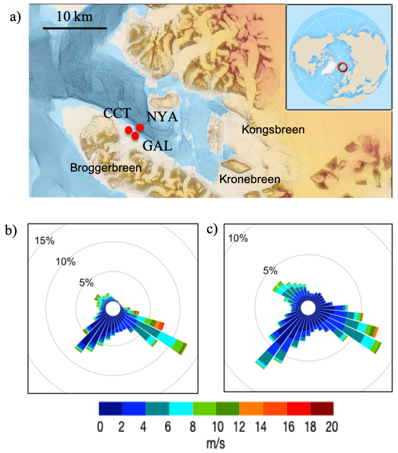
Figure 1 Map of the Kongsfjorden area (a) indicating the position of the Gruvebadet Atmospheric Laboratory (GAL), the Climate Change Tower (CCT), and Ny-Ålesund (NYA); wind rose for the cold (b) (November–April) and warm (c) (May–October) seasons derived from wind measurements performed at 2 m from the ground. Map from https://toposvalbard.npolar.no (last access: January 2023) courtesy of the Norsk Polarinstitutt.

2.2 Aerosol optical properties

Aerosol optical properties have been measured at GAL since 2010 during the warm season, while cold season measurements have been performed routinely only since March 2018. To have a complete description of the seasonal variability, this study focuses on the period 2018–2021.

Aerosol particles at GAL were sampled through a total suspended particle (TSP) inlet and the absorption coefficient was measured with a three-wavelength Particle Soot Absorption Photometer (PSAP, Radiance Research, USA) (Bond et al., 1999) operating at 467, 530, and 660 nm at a nominal flow rate of 1 L min⁻¹. Hourly absorption data were calculated from measurements with a 4 s time resolution and corrected for spot size and flow rate according to Bond et al. (1999) and Ogren (2010). We discarded measurements characterized by transmittance values lower than 0.5. Finally, absorption coefficient data were corrected for filter loading and scattering artefacts according to Virkkula (2010).

We measured the scattering coefficients with a nephelometer (M903, Radiance Research, USA) at 530 nm and corrected for illumination and truncation error according to Müller et al. (2009). Scattering coefficients at 467 and 660 nm were derived assuming a scattering Ångström exponent of 1.15 (Schmeisser et al., 2018). Absorption and scattering coefficients were adjusted to standard temperature and pressure.

From October 2019 to October 2020, a Multi-Angle Absorption Photometer (MAAP, Magee Scientific Corporation) measured the aerosol absorption coefficient at 637 nm at GAL, in parallel with the PSAP, to validate the PSAP correction algorithm. The MAAP worked at 1 min time resolution and data were averaged over 1 h. MAAP absorption coefficients were corrected according to Müller et al. (2011) and then adjusted to 660 nm to be compared with PSAP measurements, assuming an absorption Ångström exponent of 1.

2.3 Meteorological data

Meteorological measurements (temperature, pressure, relative humidity, radiation, wind direction, and wind speed) were continuously performed at the CCT (about 1 km from GAL) at a 1 min time resolution, while we used hourly precipitation, 3-hourly cloud cover, and cloud cover height measured at the Ny-Ålesund station of the Norsk Klima Service Centre (https://klimaservicesenter.no, last access: June 2022). Daily averages were calculated for all the variables, other than precipitation, for which daily cumulative values were instead derived from hourly data.

We obtained the boundary layer height (BLH) at GAL and sea level pressure maps in the Northern Hemisphere from hourly ECMWF reanalysis ERA5 data (Hersbach et al., 2020) at a spatial resolution of $\mathrm{0.25}{}^{\circ }\times \mathrm{0.25}{}^{\circ }$ (https://cds.climate.copernicus.eu/, last access: January 2023).

General circulation indices (NAO, Arctic Oscillation AO, SCAN) were downloaded from the NOAA Climate Prediction Center (https://www.cpc.ncep.noaa.gov, last access: June 2022) at daily (NAO and AO) and monthly (SCAN) time resolutions. The NAO is a measure of the difference in sea level atmospheric pressure between the Icelandic Low and the Azores High (Hurrell, 1995). A positive NAO index is associated with low pressure at high latitudes of the North Atlantic and potential transport of polluted air masses from lower latitudes (Eckhardt et al., 2003). The AO represents the strength of winds circulating around the North Pole, which are able to isolate cold air masses to the high latitudes. A low AO index indicates weaker winds, which allow the potential intrusion of warm air masses from lower latitudes. The SCAN index is based on the analysis of 700 hPa geopotential height patterns and is associated with a strong centre over Scandinavia and two weaker centres with opposite signs over western Mongolia and eastern Russia (Barnston and Livezey, 1987). Stathopoulos et al. (2021) observed that a negative SCAN phase was associated with a higher eBC concentration at the Zeppelin Observatory (Svalbard).

The daily Greenland Blocking Index (GBI) was downloaded from the Global Climate Observing System webpage (https://psl.noaa.gov/gcos_wgsp/, last access: June 2022). The GBI is the mean 500 hPa geopotential height over the region that extends from 60–80^∘ N and 20–80^∘ W and that measures the blocking pattern over Greenland.

To investigate below-cloud and in-cloud scavenging during transport to the Arctic, we downloaded daily maps of precipitation rates from the Copernicus Climate Change Service (https://cds.climate.copernicus.eu/#!/home, last access: January 2023). Daily maps ($\mathrm{1}{}^{\circ }\times \mathrm{1}{}^{\circ }$ horizontal resolution) were derived from satellite observations within the Global Precipitation Climatology Project (GPCP).

2.4 Back-trajectory analysis

Seven-day Lagrangian Analysis Tool (LAGRANTO) back-trajectories were calculated every 6 h from March 2018 to December 2021, initialized at 10 and 30 hPa above ground level at GAL (Sprenger and Wernli, 2015; Wernli, 1997). Modelling data suggest that BC atmospheric lifetime is on average 5.5 d (±2 d) (Szopa et al., 2021). Similarly, Backman et al. (2021) estimated that BC emissions affecting Arctic surface observatories can travel in the atmosphere for up to 7 d prior to reaching the receptor site (Backman et al., 2021). The 7 d duration was selected to capture BC atmospheric lifetime and removal processes along trajectories (Cremer et al., 2022; Evangeliou et al., 2016). The trajectory calculator used ERA5 as the input meteorology, with a horizontal resolution of $\mathrm{0.5}{}^{\circ }\times \mathrm{0.5}{}^{\circ }$ and a vertical resolution of 137 levels up to 1 hPa. We then reconstructed the probability residence time maps (Ashbaugh et al., 1985) to a resolution of $\mathrm{1}{}^{\circ }\times \mathrm{1}{}^{\circ }$ (Fig. S1 in the Supplement) to compare with BC emission maps and precipitation rate maps.

2.5 Generalized additive models

We used GAMs to investigate the impact of local meteorology and synoptic-scale circulation on eBC variability. GAMs do not assume a linear relationship between variables (Hastie and Tibshirani, 1986); instead, this method describes the relationship between each predictor and the dependent variable (in this case eBC concentration) as a smooth function that is generally non-parametric. The different smooth functions can be determined simultaneously, and the dependent variable is then described as a linear combination of the smooth functions, each depending on a single predictor. GAMs have been successfully employed in previous studies to investigate the dependency of particulate matter and particle number concentration on meteorological variables in urban and remote locations (Barmpadimos et al., 2012, 2011; Clifford et al., 2011; Crawford et al., 2016). In such studies, a logarithm transformation was applied to the pollutant concentration to obtain an approximate normal distribution of the dependent variable and to improve model residual interpretation (Barmpadimos et al., 2011).

We built two different GAMs to describe the eBC concentrations observed during the cold (November–April) and warm (May–October) periods, assuming that different mechanisms might control pollution variability. This assumption is corroborated by the fact that eBC observed at the Zeppelin Observatory (at about 1 km from GAL) is characterized by significantly different source regions during the warm and cold seasons, as defined above (Stathopoulos et al., 2021; Eleftheriadis et al., 2009). Furthermore, Stathopoulos et al. (2021) highlight that large-scale circulation patterns that impact the pollutant transport from lower latitudes (NAO, OA, and SCAN) shows opposite behaviours during these two periods of the year. In addition, we analysed daily rather than hourly eBC concentrations to increase the eBC signal-to-noise level and to include in the analysis covariates with time resolutions coarser than 1 h, such as general circulation indices. Finally, mild and extreme outliers were removed using the interquartile range criteria (2 out of 1026 daily data points were removed).

The logarithm of the eBC concentration was modelled according to the following equation:

$$\begin{array}{}\text{(1)}& \ln \left(\text{eBC}\right)=\sum _{j=\mathrm{1}}^p{s}_j\left(x_j\right)+\sum _{j=p+\mathrm{1}}^q{\mathit{\beta }}_j{x}_j+a+\mathit{\epsilon },\end{array}$$

where s_j is the smooth function describing the jth predictor, β_j is the linear coefficient of categorical variable x_j, p is the number of continuous variables, (q−p) is the number of categorical variables, a is the intercept, and ε is the residual.

We implemented GAM analysis using the mgcv R package (Wood, 2017). We choose penalized thin plate splines as base splines to define the smooth functions s_j, while the smoothing parameters were estimated using the restricted maximum likelihood (REML) algorithm to reduce the risk of data overfitting. Circulation indices and meteorological parameters were tested as continuous variables. We also tested precipitation and wind direction as categorical variables. In addition, we included day of the year (DOY) and truncated Julian day (tJul or continuous day count from 24 May 1968) among the investigated variables to take into account all processes that could not be explained by local meteorological variables or circulation indices, such as seasonal and annual variability of emissions and removal processes during transport. DOY ranged between 1 and 366, while tJul varied between 18 178 and 19 579.

2.6 Model definition

To build the seasonal GAMs, we first selected those variables able to explain the largest eBC variability using an iterative approach as described by Jackson et al. (2009) and illustrated in the following steps.

Step 1. Univariate GAMs were created using the explanatory variables, one at a time, and the variable associated with the largest deviance explained was selected. The deviance explained is the fraction of variance of eBC data described by the model.

Step 2. The remaining variables were added to the GAM defined in step 1, one at a time, and the deviance explained was re-calculated. The model characterized by the highest deviance explained was chosen.

Step 3. The variable selected in step 1 was removed and replaced by the remaining variables. If the new deviance explained was higher than the one from step 2, the new model was retained. If two variables were associated with a similar increase in the deviance explained, the one characterized by a higher significance (i.e. a lower p value) was selected.

Step 4. To test the model robustness, we verified that all the variables included in the model were significant at least at the 95 % significance level.

Step 5. Multi-collinearity of GAM covariates should be avoided, as this would make it difficult to discriminate the impact of the different variables and would introduce redundancy into the model. To test multi-collinearity, when a new variable was added to the model, the variance inflation factor (VIF) was calculated as follows:

$$\begin{array}{}\text{(2)}& \text{VIF}={\displaystyle \frac{\mathrm{1}}{\mathrm{1}-r^{\mathrm{2}}}}.\end{array}$$

r is the Pearson correlation coefficient that defines the correlation of the last added variable against all the other variables already included in the multivariate GAM (Barmpadimos et al., 2011). As a general rule, a VIF equal to 1 corresponds to no correlation, while a VIF between 1 and 5 indicates a weak correlation. In this study, if the VIF exceeded 2.5, the variable was not added to the model and the covariate with the second highest deviance explained was tested. A VIF equal to 2.5 was chosen because it corresponds to a coefficient of determination of 0.6, which is the maximum collinearity among covariates that was considered acceptable.

Step 6. We repeated steps 2 to 5 until the deviance explained increase was smaller than 2 %.

Finally, we tested the normality (normal distribution of the residuals around zero), homoscedasticity (constant variance of the residuals), and linearity (linear correlation of the predicted versus observed values) of the model results.

2.7 BC emissions

We derived BC monthly emissions from anthropogenic sources using EDGARv6.1 (Emissions Database for Global Atmospheric Research) (https://edgar.jrc.ec.europa.eu/index.php/dataset_ap61, last access: July 2022) developed by the Joint Research Center of the European Commission (Crippa et al., 2019). Monthly gridded emissions for different activity sectors are available for the years 1970–2018 at a spatial resolution of $\mathrm{0.1}{}^{\circ }\times \mathrm{0.1}{}^{\circ }$. We used the most recent data, i.e. 2018 emissions, as representative of the period 2018–2021. The following emission sectors were considered: power industry, refineries and transformation industry, combustion for manufacturing, residential combustion, road transportation, other transportation, and shipping. These sectors, together with agricultural burning, account from more than 94 % of the total BC emissions in Europe, Russia, Canada, and the USA, excluding the land use, land use change and forestry (LULUCF) sector (Fig. S2).

The EDGAR inventory does not include the contribution from LULUCF, and thus we derived BC monthly emissions from open burning, including agricultural waste burning, using the Global Fire Emission Database (GFED; https://www.globalfiredata.org, last access: January 2022). The GFED is based on fire activity and vegetation property data from satellite observations (Giglio et al., 2013). We employed the GFED4s version, which also includes small fires (Randerson et al., 2012; van der Werf et al., 2017). For each grid cell with spatial resolution $\mathrm{0.25}{}^{\circ }\times \mathrm{0.25}{}^{\circ }$, we calculated BC emissions by multiplying the total dried matter emissions ($\mathrm{kg}{\mathrm{m}}^{-\mathrm{2}}{\mathrm{month}}^{-\mathrm{1}}$) by the grid cell area (m²) and by the BC emission factors (grams of BC per kilograms of dried matter) of the six different BC sources included in the database: savanna, grassland and shrubland fires, boreal forest fires, temperate forest fires, tropical deforestation and degradation, peat fires, and agricultural waste burning (Akagi et al., 2011; Andreae and Merlet, 2001).

To select the regions that contributed to the eBC measured on Svalbard, we overlapped the monthly emission maps from EDGAR and GFED with the back-trajectory residence time maps calculated for the corresponding month from the LAGRANTO analysis tool.

3 Results and discussion

3.1 PSAP data validation

eBC is derived from the aerosol absorption coefficient (B_abs) measured by a PSAP, whose measurements were corrected for filter loading and light scattering induced by particles deposited on the collection filter. The correction algorithm, developed by Virkkula (2010), is validated here by comparing hourly PSAP data with co-located MAAP measurements during 1 year from October 2019 to October 2020. The MAAP is employed as a reference technique since it automatically corrects the aerosol absorption coefficient for filter loading and scattering by measuring, in addition to light attenuation, the backscattering of particles on the filter (Müller et al., 2011; Petzold and Schönlinner, 2004).

Figure 2 compares the time series of hourly PSAP and MAAP absorption coefficients at 660 nm. During the intercomparison period, the absorption coefficient ranged between the detection limit (0.013 Mm⁻¹ for MAAP and 0.002 Mm⁻¹ for PSAP) (Asmi et al., 2021) and 2.8 Mm⁻¹, with an average value of 0.22 Mm⁻¹. PSAP agrees well with the MAAP data, with a Pearson coefficient of 0.93. The linear fit is characterized by a slope equal to 0.982 (±0.005) and an intercept of 0.042 (±0.002). The relationship between the two time series is comparable to the one reported by Asmi et al. (2021) during an intercomparison field experiment in northern Finland, with absorption coefficient values similar to those observed during this study. The agreement between the MAAP and PSAP time series corroborates the suitability of the correction algorithm described in Sect. 2.2 (Virkkula, 2010).

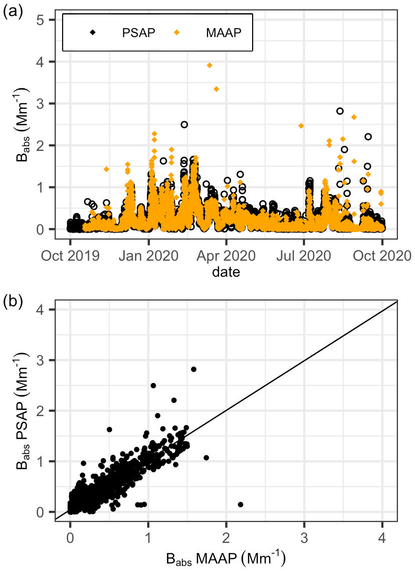
Figure 2 Time series of the aerosol absorption coefficient at 660 nm (B_abs) measured by a Particle Soot Absorption Photometer (PSAP in black) and a Multi-Angle Absorption Photometer (MAAP in orange) at Gruvebadet (panel a), together with comparison of B_abs measured by the two instruments during the intercomparison experiment from October 2019 till October 2020 (panel b).

3.2 eBC seasonality

eBC was then derived from the absorption coefficient time series at 660 nm, assuming a constant mass absorption cross section (MAC) equal to 10.2 m² g⁻¹, in agreement with the MAC calculated by Ohata et al. (2021) with instrument techniques similar to the ones employed in this study (see Sect. S1 and Table S1 in the Supplement).

Figure 3 shows the monthly variability of eBC concentrations from 2018 to 2021. Only months characterized by an hourly temporal coverage larger than 50 % are reported to guarantee data representativeness (Rose et al., 2021). eBC concentrations averaged 22 ng m⁻³ (±20 ng m⁻³) during the cold season (November–April) and 11 ng m⁻³ (±11 ng m⁻³) during the warm season (May–October). The highest eBC monthly averages were observed from January to April, corresponding to the Arctic haze period, while the lowest ones were recorded between June and October. The observed eBC seasonality agrees with previous studies from Svalbard (Eleftheriadis et al., 2009; Stathopoulos et al., 2021). The average eBC concentrations measured at the Zeppelin Observatory, at about 1 km from GAL and at 474 m altitude, averaged 21 and 7 ng m⁻³ in the cold and warm seasons, respectively, in the period 2011–2015 (Stathopoulos et al., 2021). Higher seasonal averages were instead reported in previous years (Eleftheriadis et al., 2009), in agreement with a decrease in BC concentrations in the Arctic during the last 3 decades (Schmale et al., 2022). Increased vertical mixing in the lower troposphere and more frequent precipitation during summer promote aerosol dilution and removal processes in the warmer period, leading to a reduction in the surface eBC concentration (Stohl, 2006; Garrett et al., 2011). Furthermore, the extension of the Arctic front towards lower latitudes during the cold period facilitates the transport of polluted air masses from populated regions in northern Europe and Russia (Quinn et al., 2015; Stohl, 2006).

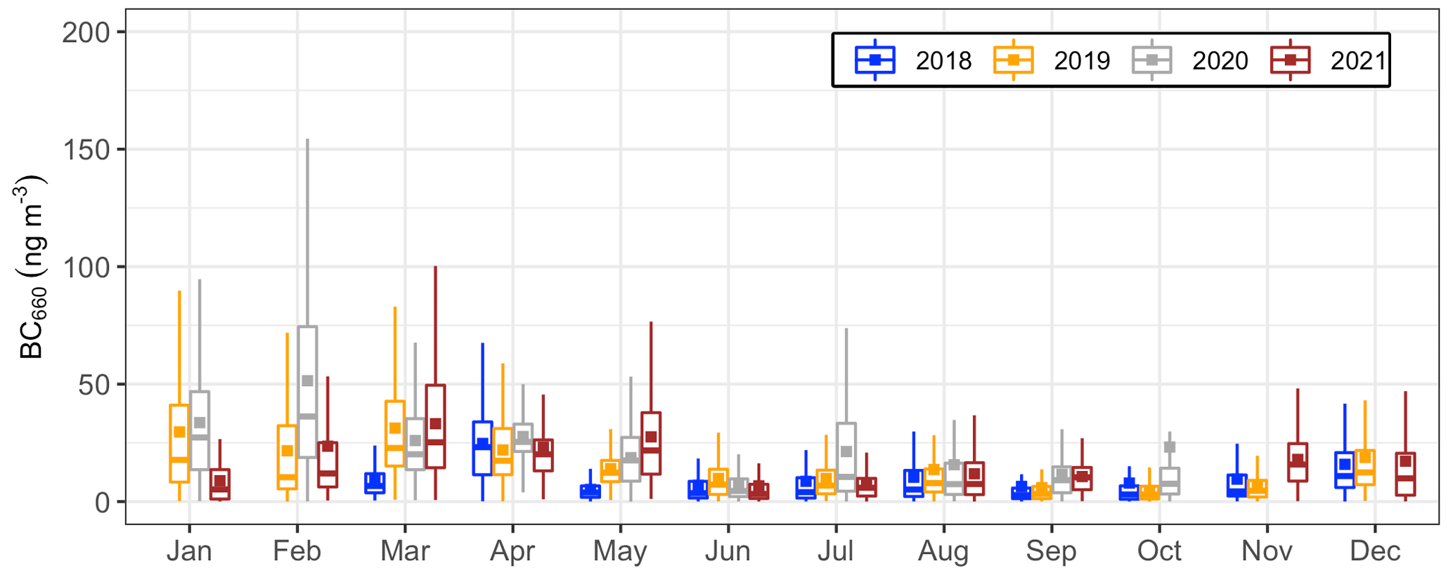
Figure 3 Box–whisker plot of the equivalent black carbon (eBC) concentration according to months and years. The lower and upper box boundaries correspond to the 25th and 75th percentiles, respectively, vertical lines extend to the minimum and maximum without outliers, horizontal lines inside the box indicate the medians, and squares correspond to the averages.

Figure 3 shows some variability of the eBC monthly statistics from one year to another. Statistically significant differences were observed mainly during the cold and transition periods. In 2018, March and May showed significantly lower eBC concentrations compared to the same months of the other investigated years, while in 2020, February and October were characterized by slightly larger concentrations. January and November 2021 exhibited lower and higher eBC values relative to the other monthly means, respectively. During the warm period, the largest difference was observed in July 2020, when the mean eBC concentration was higher compared to the same months of the remaining analysed years.

3.3 Analysis of drivers controlling eBC variability

In this section we use GAMs to identify and discuss the explanatory variables that best describe the variability of eBC in the European Arctic and to understand how they link to the synoptic-scale circulation and local meteorology.

To facilitate the interpretation of the covariate effect, we first investigated the correlation among them. Figure S3 reports the Pearson correlation matrices for the cold and warm periods. Wind speed correlated with boundary layer height, because local wind promoted atmospheric vertical instability. As expected, the NAO and AO correlated with each other and anticorrelated with the GBI, since they describe opposite pressure fields (Hanna et al., 2014). During the cold season, atmospheric pressure correlated with the GBI and anticorrelated with the AO, because a positive GBI phase and a negative AO phase are characterized by a high-pressure system over the Arctic region. The correlation weakened in the warm season due to the lower variability of the GBI and AO indices.

3.3.1 Cold season

Table 1 reports the covariates selected for the cold season GAM together with the deviance explained by the model after the addition of each variable and the corresponding p values. Low p values indicate a high significance of the relationship between ln(eBC) and the explanatory variable. The smoothed functions describing the dependency of the eBC on each covariate are shown in Fig. 4. In each box, the vertical axis shows the additive effect of one specific covariate on the eBC concentration as a function of the covariate values reported on the horizontal axis.

Table 1 Explanatory variables of cold season and warm season GAMs. The order of the variables corresponds to the selection order during the GAM definition. Deviance explained is the cumulative value of each variable and the preceding ones, while the p values are indicative of each variable's statistical significance (for all variables larger than 99.9 %).

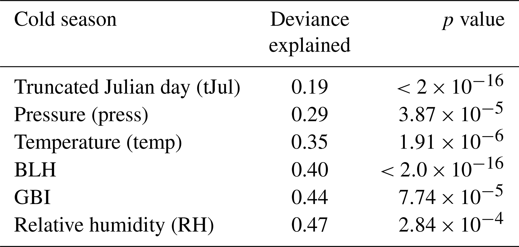
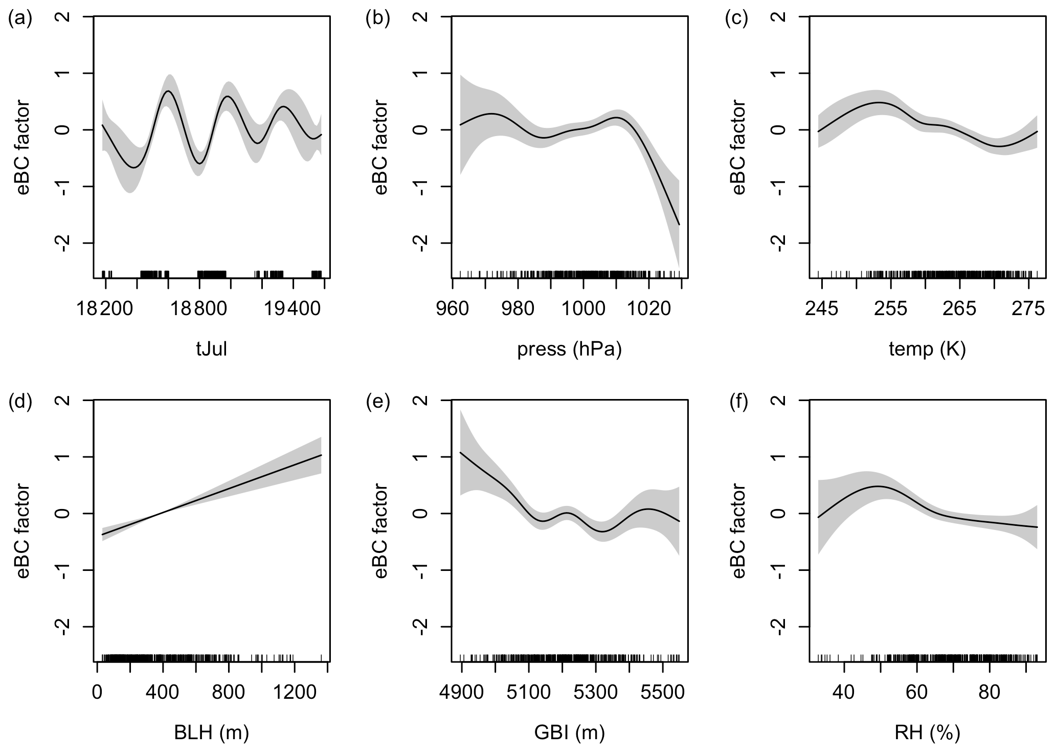
Figure 4 Smooth functions of the variables contributing to defining the eBC concentration in the cold season GAM. In each plot, the y axis reports the change in the eBC concentration relative to the seasonal average; an eBC factor equal to +1 corresponds to an increase in the eBC concentration equal to 100 % relative to the cold season average. The tick marks on the x axis show the distribution of the predictor values across their variability ranges.

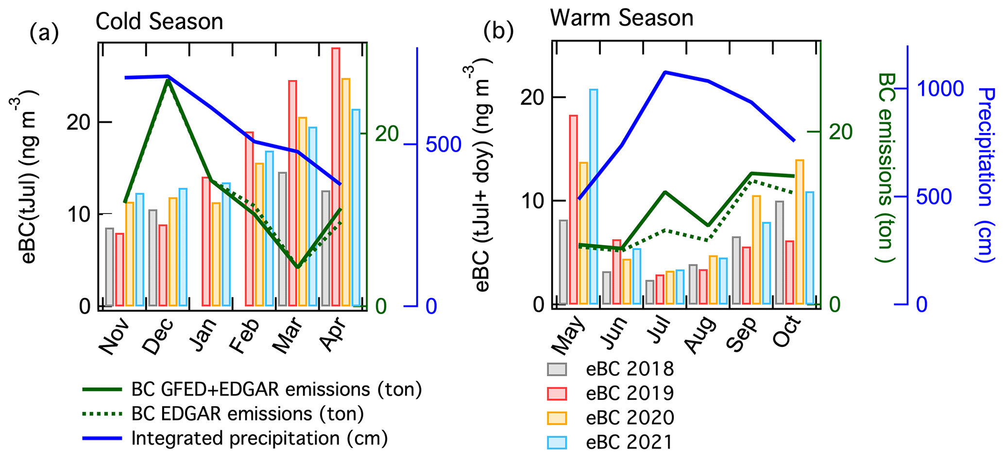
Figure 5 eBC concentration predicted by truncated Julian day in the cold season (panel a) and by truncated Julian day together with DOY in the warm season (panel b); the blue lines indicate the monthly precipitation integrated along back-trajectories, while the green lines correspond to BC emission monthly averages excluding (dotted lines) and including (continuous lines) open burning emissions.

The first variable selected for the definition of the cold season GAM was tJul, which alone accounted for 19 % of the eBC variance (Fig. 4a). Although DOY was the second variable with the highest deviance explained in the univariate models (16 %), it was not selected as an explanatory variable during the multivariate model definition (Sect. 2.6), indicating that truncated Julian day already accounted for the seasonal variability that would have been described by the DOY. To clarify the impact of truncated Julian day, Fig. 5a reports the monthly average of eBC concentrations derived by the GAM using this covariate alone. Truncated Julian day combines the effects of drivers that are characterized by a clear seasonal and interannual variability. On average, modelled eBC concentrations were similar in November and December and increased by a factor of 2 from November to April, with some interannual differences. Previous studies attributed BC seasonal variability to the increase in wet scavenging efficiency in the colder months (Arctic haze) and the retreat of the Arctic front during the warmer months, the latter reducing the source regions potentially able to impact the Arctic air quality (Stohl, 2006; Garrett et al., 2011; Freud et al., 2017). To investigate the relative significance of these two effects, Fig. 5a reports the monthly precipitation and BC emissions integrated along trajectories. BC monthly emissions were calculated by multiplying the back-trajectory residence time maps from LAGRANTO analysis by the BC emission flux maps, and thus they take into account the Arctic front seasonal variability. BC emissions did not explain the model eBC trend; in fact, they increased from November to December and then decreased progressively during the following months. Instead, the integrated precipitation was comparable in November and December and then decreased progressively from December to April, showing an opposite trend compared to the eBC-predicted values. Monthly averages of eBC derived from truncated Julian day weakly anticorrelated with the precipitation rate along back-trajectories ($r=-\mathrm{0.43}$), whilst the predicted eBC showed no link with BC emission variability ($r=-\mathrm{0.11}$) (Fig. S4), indicating that scavenging efficiency had a stronger impact on eBC seasonality than emission variability. The anticorrelation (negative r value) indicates that an increase in precipitation rate was associated with a decrease in surface eBC concentration, as expected due to wet scavenging.

The second selected covariate was surface atmospheric pressure, which explained 29 % of the eBC variance in combination with truncated Julian day (Fig. 4b). Statistically significant effects were observed for pressure above 1010 hPa. In particular, when pressure increased from 1010 to 1025 hPa, eBC decreased by 70 %. The threshold value of 1010 hPa is relatively high when compared to the average surface pressure recorded during the cold season (1000 hPa) and the average values reported for the same location in previous years (about 1006 hPa) (Maturilli et al., 2013; Mazzola et al., 2016). Figure S5 reports the average sea level pressure (SLP) maps derived from ERA5 re-analysis and corresponding to the periods characterized by pressure at GAL higher than 1010 hPa and the entire cold season. In the first case, the SLP over the Arctic was higher than the average, and a centre of high pressure was localized over Svalbard. The difference in the local SLP corresponds to substantially different synoptic-scale SLP patterns, and hence local pressure can be considered a proxy for large-scale synoptic circulation. High-pressure patterns over the Arctic in winter weaken westerly flows over the Atlantic Ocean and prevent the advection of air masses from the European continent to the higher latitudes (Maturilli and Kayser, 2017). Thus, the reduction in eBC concentration at high surface pressure observed in this study is explained by a blocking of pollution transport from lower latitudes.

The third selected variable was surface temperature, explaining 35 % of the eBC variance, in combination with truncated Julian day and surface pressure (Fig. 4c). A significant impact of this covariate was observed at values between 255 and 270 K (corresponding to 75 % of the data points), when a 10 K temperature rise led to a drop in eBC concentration by 32 % on average. Increase in temperature corresponds to the transport of warmer and more humid air masses to Svalbard (Maturilli and Kayser, 2017; You et al., 2022). The cold season mean specific humidity was 1.5 g kg⁻¹, while it averaged 2.2 g kg⁻¹ when the temperature was higher than 265 K. The relative increase in specific humidity suggests that air masses reached Svalbard after spending most of their time over the ocean rather than over the continental areas, where most of the emissions originate. Figure 6a and c compare the average sea level pressure over the Northern Hemisphere and the residence time of back-trajectories reaching GAL when local temperature was lower or higher than 265 K. Under colder conditions, a strong pressure gradient between Siberia and the Eurasian Arctic supported the transport of air masses from northern Siberia to higher latitudes, favouring the transport of air pollutants to Svalbard. Conversely, when temperature at GAL was relatively higher, the Siberian anticyclone weakened while the pressure over the European Arctic increased, blocking the transport of air masses from the polluted European and Asian mainland while favouring transport from the Atlantic Ocean sector. Figure 6b and d report the probability residence time maps corresponding to the two conditions and clearly show that when the temperature at GAL was higher, air masses spent more time over the Fram Strait; this led to a decrease in the observed eBC concentration.

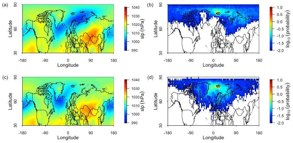
Figure 6 Average sea level pressure map and residence time probability map when temperature at GAL was lower than 265 K (panel a and b, respectively) and higher than 265 K (panel c and d, respectively) during the cold season. Residence time probability maps are based on 7 d back-trajectories.

BLH increased the deviance explained by the GAM up to 40 % (Fig. 4d). The effect of this covariate was particularly significant when BLH was shallow (below 600 m). In fact, eBC increased by about 40 % when BLH increased from 100 to 600 m. Rader et al. (2021) observed that anthropogenic aerosol is transported great distances towards the European Arctic in the lower free troposphere, and then it might mix down in the boundary layer in areas with complex orography such as Ny-Ålesund in Svalbard. It follows that a higher boundary layer favours downward mixing of BC from the free troposphere, increasing the observed concentrations at sea level. Furthermore, in the cold season, shallow boundary layer conditions at GAL were dominated by very weak flow from the south-west, while increasing BLH was associated with the shift in the prevailing wind direction towards east-southeast and an increasing wind speed (Fig. S6a–d). Winds from east-southeast correspond to the descending movements of air masses along the slope of the glaciers at the western edge of the Kongsfjord, promoted by sea breeze and terrain orography (Sjöblom et al., 2012). It is likely that such descending air masses contributed to the transport of pollutants from the lower free troposphere towards GAL.

The GBI and relative humidity (RH), the two remaining variables included in the cold season GAM, increased the deviance explained by the model up to 47 % and had a small effect on the eBC level (Fig. 4e and f, respectively). eBC concentration increased when the GBI was smaller than 5100 m (Fig. 4e) due to the weakening of the blocking system triggered by the high pressure over Greenland (Dekhtyareva et al., 2022). The effect of relative humidity above 50 % was a slight reduction in eBC concentration, likely due to the local in-cloud and below-cloud scavenging (Fig. 4f). When relative humidity was lower than 50 %, the effect on eBC was characterized by a large uncertainty due to the small number of data points in this humidity range.

3.3.2 Warm season

Table 2 shows the covariates selected for the warm season GAM (May–October), while Fig. 7 reports the smoothed functions describing the link between eBC and the selected covariates.

Table 2 As in Table 1 but for the warm season. The p values are indicative of each variable's statistical significance (${}^{\ast \ast }$ corresponds to a significance larger than 99.9 % and ^∗ to a significance larger than 95 %).

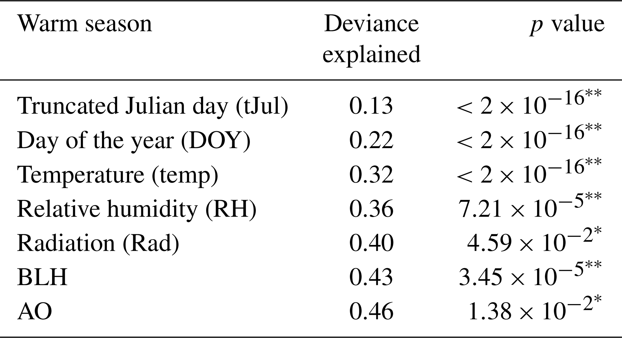
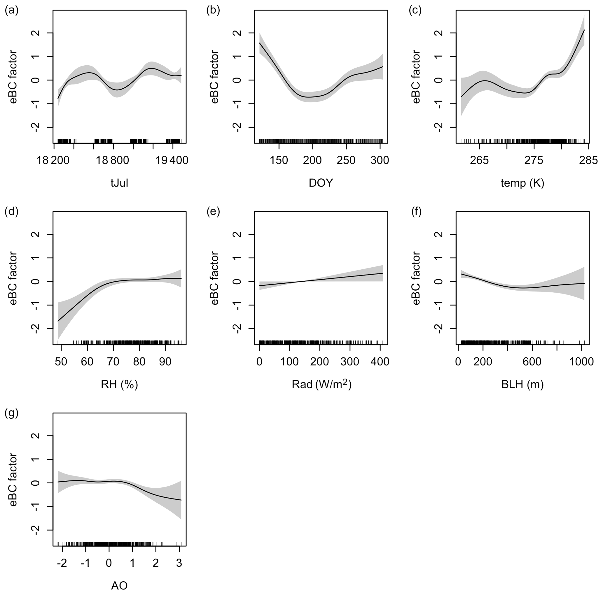
Figure 7 Smooth functions of the variables contributing to defining the eBC concentration in the warm season GAM.

The first two selected covariates were truncated Julian day and DOY, which together explained 22 % of the eBC variance (Fig. 7a and b, respectively). We discuss them together as they describe processes characterized by a smooth interannual and seasonal variability. The selection of both truncated Julian day and DOY as explanatory variables indicates larger interannual differences in the seasonal trends compared to what was observed during the cold season, when the selection of a truncated Julian day excluded DOY from the model. Figure 5b reports the modelled eBC concentration derived from DOY and truncated Julian day. The monthly modelled eBC averages show minimum values in July and then increase during the following months, with different rates during the different years. On average, estimates of eBC concentrations decreased by 80 % from May to July and then increased by 53 % to 77 % from July to October. The seasonal variability of BC emissions is not linked to the modelled eBC (Fig. 5b). Conversely, precipitation integrated along back-trajectories increased by a factor of 2 from May to July and then decreased till the end of summer, mirroring the trend of modelled eBC. Monthly averages of modelled eBC clearly anticorrelated with precipitation ($r=-\mathrm{0.70}$), indicating that eBC variability was strongly affected by the efficiency of removal processes during transport. This was particularly evident in the warm season, which showed higher precipitation values than the cold season (Fig. S4). The correlation with monthly emissions was instead negligible ($R=-\mathrm{0.13}$).

The third selected variable was temperature, which together with truncated Julian day and DOY explained 32 % of the eBC variance (Fig. 7c). Statistically significant effects were observed for temperatures above 275 K, when eBC increased by about 88 % when temperature increased by 10 K. Higher temperature in the Arctic could be due to diabatic warming, adiabatic warming due to subsidence, or intrusion of air masses from lower latitudes (Papritz, 2020). The analysis of meteorological parameters during transport shows that only a limited number of back-trajectories arriving at GAL during warmer days (average temperature higher than 278 K) experienced diabatic warming before arriving at the observatory (10 %). Furthermore, we investigated adiabatic warming due to subsidence based on the maximum pressure increase experienced by the back-trajectories during the last 2 d before reaching GAL (Binder et al., 2017). The frequency distribution of maximum pressure rise in Fig. 8a shows a slightly higher frequency of back-trajectories undergoing a pressure increment between 50 and 100 hPa on warmer days compared to colder days. The pressure change indicates the subsidence from the lower free troposphere just before reaching the observatory. Finally, to study the intrusion of air masses from lower latitudes, the histograms in Fig. 8b report the frequency distribution of the minimum latitudes reached by the back-trajectories up to 7 d before arriving at GAL as a function of the average daily temperature. The histogram comparison indicates that it was more likely that air masses originated from regions south of the 70th parallel during warmer days (62 % of the time) than during colder days (40 % of the time). To further validate these results, Fig. S7a and c show the average sea level pressure, while Fig. S7b and c report the residence time maps corresponding to 7 d back-trajectories reaching GAL during the warm season. Colder temperatures (T<278 K, 69 % of the time) at the observatory corresponded to the arrival of air masses that spent more time over the Arctic Ocean and Greenland coasts (Fig. S7e). On the other hand, warmer temperature periods (T>278 K, 31 % of the time) were characterized by a lower-pressure system over the North Atlantic Ocean that favoured the transport of air masses from lower latitudes and through northern Europe and Russia (Fig. S7e). To summarize, the higher eBC concentrations observed at GAL during warmer days can be due to the effective transport of polluted air masses from lower latitudes as well as the intrusion of pollution from the lower free troposphere.

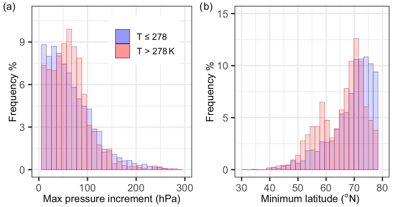
Figure 8 Histograms reporting the frequency of back-trajectory maximum pressure increases during the last 48 h before reaching GAL (panel a) and minimum latitude reached during the 7 d before reaching the observatory (panel b). Back-trajectory data of colder days are reported in blue and those of warmer days in red, while the purple area corresponds to the overlapping region of the two histograms.

RH was selected at the fourth step and increased the model deviance explained up to 36 % (Fig. 7d). Dry conditions at GAL (RH below 70 %) corresponded to a reduction in eBC concentration by about 30 %. No effect was observed for higher RH. The average specific humidity was 2.5 ± 1.1 and 3.9 ± 1.0 g kg⁻¹ when RH was lower and higher than 70 %, respectively. Figure S8 reports the analysis of specific humidity and pressure along back-trajectories arriving at GAL under dry and wet conditions. In both cases, specific humidity progressively increased along the trajectories, indicating that wet scavenging could not explain the lower eBC concentrations observed on drier days. Conversely, low RH at GAL corresponded to the arrival of air masses that spent most of their time at higher altitudes compared to air masses arriving under wetter conditions. Likely, air masses moving at higher altitudes could not collect water and pollutants from the surface of the ocean and land and resulted in a lower specific humidity and a lower eBC concentration at GAL.

The next variable included in the warm season GAM was radiation (Fig. 7e), which brought the model deviance explained to 40 %. eBC concentration increased by 23 % when radiation increased from 50 W m⁻² to more than 100 W m⁻², likely due to the decreased probability of aerosol scavenging from low-level clouds and drizzle. This is confirmed by the reduction in the radiation impact when cloud height was added to the model as a factor covariate. In particular, the effect of low-level clouds (clouds below 500 m) in the warm period was a reduction in eBC concentration by 23 % on average. Low-level clouds are usually associated with rain and drizzle, with the latter not well captured by cumulative hourly precipitation measurements (Nystuen, 1999).

The last covariates added to the model were BLH and AO (Fig. 7f and g, respectively), which brought the deviance explained up to 46 %. The warm season BLH had an opposite effect compared to the one observed in the cold season. In fact, when BLH decreased from 400 m to less than 100 m, the eBC concentration increased by about 60 % (Fig. 7f). The effect of BLH is likely controlled by the dominating wind circulation during shallow boundary layer conditions (Fig. S6e–g). When BLH was lower than 100 m, circulation was mainly characterized by winds from the east and east-southeast. This wind pattern was triggered by air masses descending along the slope of the glaciers at the western edge of the Kongsfjord (Sjöblom et al., 2012), which promoted the transport of pollutants form higher altitudes and their intrusion into the shallow boundary layer (Graßl et al., 2022). Furthermore, the weak wind speed favoured eBC accumulation. Days with BLH between 100 and 400 m were instead characterized by progressively higher wind speed and more frequent winds from the south-west (from the Brøggerbreen glacier) and north-east (from the entrance of the fjord). Likely, the lower altitude of the mountain ridge to the south-west compared to the western edge of the fjord did not allow effective transport of pollutants from the lower free troposphere. Similarly, the entrance of air masses from the ocean direction at sustained wind speed (2 to 8 m s⁻¹) contributed to pollutant dispersion. Finally, for a BLH larger than 400 m, the model uncertainty increased and the effect of BLH became less clear.

The effect of the AO (Fig. 7g) goes in the same direction as the NAO impact observed at the Zeppelin Observatory during the warm season, with higher eBC during the AO (or NAO) negative phase (Stathopoulos et al., 2021). A negative AO phase corresponds to weaker polar winds and potential intrusion of polluted air masses from lower latitudes. In addition, Christoudias et al. (2012) reported that a positive NAO phase is associated with increased precipitation over northern Europe. Since the NAO and AO phases correlated during the investigated period, the reduction in eBC during high AO periods could also be attributed to the enhanced BC scavenging during transport to the Arctic.

3.4 Unaccounted-for synoptic-scale circulation patterns and model performance

Stathopoulos et al. (2021) observed that eBC variability at the Zeppelin Observatory (Svalbard), at about 1 km from GAL, was affected by SCAN. SCAN is a measure of the pressure difference between northern and southern Europe, and a positive index indicates a blocking activity over Scandinavia and western Siberia. Negative SCAN values are generally associated with a higher eBC concentration at Svalbard due to favourable pollution transport from northern Eurasia, especially in the cold period (Stathopoulos et al., 2021). The effect was less clear during the warm season, although the authors reported a link between a negative SCAN phase and a high eBC concentration during the most recent years (Stathopoulos et al., 2021). Since SCAN was available at a monthly time resolution, it was not included in the GAM definition, but we investigated its effect on monthly eBC concentrations and model biases. During this study, eBC monthly averages were larger for the negative SCAN phase and smaller for the positive phase, in agreement with the impact described by Stathopoulos et al. (2021). SCAN explained only 4 % of the model bias variability in the cold season (Fig. S9a), indicating that the effect of such an index was already captured by one of the variables included in the model, likely temperature. In fact, the average sea level pressure map associated with a high surface temperature and a high eBC concentration (Fig. 6a) corresponds to the SCAN negative-phase pressure pattern. Conversely, SCAN explained 31 % of the model bias variability in the warm period (Fig. S9b). In particular, months with a strong negative SCAN index (smaller than −2) were associated with the largest monthly biases. Adding SCAN to GAM would likely help to improve GAMs in the warm period.

To test the impact of a potential unaccounted-for synoptic-scale circulation pattern in the cold period, we first calculated the average cold season SLP map from 30 to 90^∘ N, we then calculated the SLP anomalies (the difference between each daily map and the cold period average map), and finally we investigated the correlation between the anomaly time series in each cell and the time series of the GAM residuals (the differences between the measured eBC concentration and the eBC simulated by the cold season model). Figure 9 reports the map of the Pearson correlation coefficients and shows that higher residuals were associated with low-pressure anomalies over Scandinavia and western Russia and with high-pressure anomalies over the Atlantic Ocean between Spain and the Azores. The lowest Pearson correlation coefficient (r) between residual time series and SLP anomalies was observed in the region between 55 and 65^∘ N and between 42 and 50^∘ E ($r=-\mathrm{0.21}$), while the highest correlation was reported for the region between 30 and 45^∘ N and between 10 and 22^∘ W (r=0.19). We re-ran the GAM, adding the SLP difference between these two regions as a predictor variable. The SLP difference did not reduce the statistical significance of the other covariates contributing to the model but slightly attenuated their effect. In particular, when pressure increased from 1010 to 1025 hPa, eBC decreased by 63 % instead of 70 %, while the temperature increase from 255 to 265 K reduced the eBC concentration by 24 % instead of 32 %. Finally, eBC increased by 33 % instead of 40 % when BLH increased from 100 to 600 m.

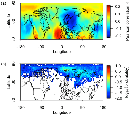
Figure 9 Correlation map of SLP anomalies during the cold period and GAM residuals during the same season (panel a). Residence time probability map for 7 d back-trajectories when the pressure gradient between western Russia and the Atlantic Ocean was larger than 20 hPa (panel b).

The use of an SLP gradient as a covariate increased the deviance explained by the model significantly (from 47 % to 52 %). The eBC dependency on the pressure gradient was linear and the average eBC concentration increased by 67 % when the pressure difference increased from values lower than −10 hPa to higher than 20 hPa (i.e. lower pressure over western Russia and higher pressure over the Atlantic). Figure 9b reports the probability time map of the back-trajectories reaching GAL when the pressure difference between the two regions was larger than 20 hPa. The map shows that, for larger pressure gradients, trajectories moved over central and northern Russia before reaching the Arctic. The high-pressure difference between the two regions likely accelerated the transport of air masses over southern Europe, and then the low-pressure system over western Russia favoured rapid movement of such air masses towards the Arctic. These results indicate that transport through northern Russia is a very effective pathway for pollution into the European Arctic.

The deviances explained by cold and warm season GAMs were comparable to the ones previously published for models investigating particulate matter (PM) variability. For example, the deviance explained by GAMs describing fine and coarse aerosol mass concentrations at European urban and rural sites ranged between 28 % and 75 % (Barmpadimos et al., 2012), while consistently smaller values were reported in remote areas (38 %–45 %) (Barmpadimos et al., 2011). eBC hourly concentrations at GAL were often of the same order of magnitude as the analytical quantification limit (2 ng m⁻³, assuming the limit of quantification to be equal to 10 times the blank standard deviation from Asmi et al., 2021). As a consequence, the measurement uncertainty might reduce the fraction of variance that could be described by the model, leading to a relatively lower deviance explained (Barmpadimos et al., 2012). The mean square errors (MSEs) were 2.8 and 2.6 ng m⁻³ in the cold and warm seasons, respectively. To investigate GAM performance, Fig. 10a and b report the scatter plots of modelled versus observed concentrations during the two seasons. Most of the points were close to the 1-to-1 line, and the fraction of data with a modelled-to-observed eBC ratio between 0.5 and 2 (Chang and Hanna, 2004) was equal to 72 % and 71 % in the cold and warm periods, respectively. GAMs underpredicted eBC during both seasons for concentrations larger than 50 ng m⁻³, likely due to the difficulties the model has in describing the behaviour of an underrepresented eBC concentration range. In fact, the eBC daily average was larger than 50 ng m⁻³ only during 9 % and 1 % of the time in the cold and warm seasons, respectively. Figure 10c shows that, overall, the model reproduces well the observed seasonal and interannual variability of the monthly eBC averages (Fig. 10c).

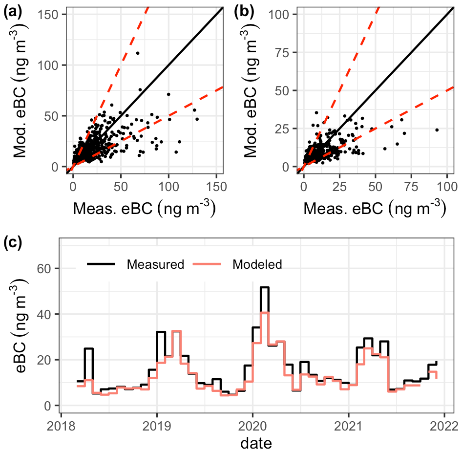
Figure 10 Comparison between measured and modelled eBC concentrations during the cold (panel a) and warm (panel b) seasons; the red dotted line indicates the factor of 2 area. Panel (c) shows the time trends of modelled and measured eBC monthly averages.

4 Conclusions

Black carbon is a short-lived climate forcer that plays a crucial role in the Arctic climate system. Nevertheless, most climate models still fail in reproducing its atmospheric concentration seasonal changes at high latitudes. We analyse equivalent black carbon (eBC) concentration variability during 4 years at the Gruvebadet Atmospheric Laboratory, in the Svalbard archipelago, to understand the impact of local- and synoptic-scale processes on black carbon seasonality in the European Arctic.

To study eBC variability, we deployed generalized additive models that allowed us to describe eBC concentration as the sum of multiple factors, each of them depending on a single covariate, without assuming a linear relationship with the predicted variable (eBC). We tested local meteorological observations, ERA5 reanalysis products, and general circulation indices as covariates. Compared to previous studies that investigated the impact of a single variable or process at a time (Stathopoulos et al., 2021; Eckhardt et al., 2003), the GAM approach allowed us to evaluate simultaneously the effect of multiple variables, disentangling their relative contribution. Both cold and warm season eBC concentrations were equally well explained by the GAMs.

eBC concentration showed clear seasonal differences, with higher values in late winter and spring and lower concentrations in summer. We observed a weak to moderate correlation between the seasonal variabilities of eBC and removal processes taking place at the regional scale during transport from lower latitudes. We observed that precipitation amount integrated during transport is a key factor controlling aerosol seasonality, especially during the warm season, when precipitation rate is higher. On the other hand, the link between emission variability and eBC concentration was not as clear, even if BC emission inventories were used in connection with back-trajectories, to account for the changes in air mass circulation patterns. Although with some caution due to the fact that anthropogenic BC emissions were only available for a single reference year (i.e. 2018), the results presented here agree with the conclusions, based on tracer analysis, that wet scavenging controls the seasonal cycle of pollutant concentrations observed in the Arctic (Garrett et al., 2011).

Local temperature explained a significant fraction of the eBC variance during both the cold and warm periods but with opposite effects. During the cold season, higher concentrations were observed for temperatures at GAL lower than 265 K. Stohl (2006) reported that effective pollution transport to the Arctic lower troposphere requires the penetration of the polar dome from sideways. This route is possible for air masses characterized by low potential temperature; 85 % of the back-trajectories reaching GAL during cold days experienced diabatic cooling (potential temperature decrease) up to 1 d before reaching the observatory. The average cooling rate was −1.6 K d⁻¹, which is higher than the rate expected from radiative cooling but in agreement with diabatic cooling due to contact with snow-covered ground (Stohl, 2006). This result agrees with back-trajectories showing the potential impact of air masses from northern Siberia during colder days.

During the warm season, eBC concentration almost doubled when temperature increased from 275 to 285 K. Back-trajectory analysis confirms that higher temperatures in Svalbard corresponded to the intrusion of polluted and warmer air masses from lower latitudes, where BC sources are located. Warm air intrusions have been particularly investigated during winter for their contribution to reduction in sea ice concentration and impact on cloud radiative forcing (Woods et al., 2013; Woods and Caballero, 2016; Zhang et al., 2023). By contrast, studies of summer events are limited, although the presence of sunlight in this season makes climate implications even more complex (Tjernström et al., 2019; You et al., 2021). Recently, a few studies reported a correlation between pollution transport to the Arctic with warm air intrusion based on the analysis of single events in summer and late spring (Bossioli et al., 2021; Dada et al., 2022). Our results verified the consistency of such a pattern with longer time series and highlighted the need to further investigate the implications of warm air intrusion in the warm periods, when the background aerosol concentration is lower, and these events can alter substantially aerosol population climate-relevant properties (Dada et al., 2022).

Among synoptic-scale meteorology descriptors, SCAN might contribute to the temporal eBC variability in the warm seasons, although the lack of a daily time resolution for this index did not allow us to test it as a predictor in the GAM. In the cold period, higher eBC concentrations were observed for a positive pressure gradient between northern and southern Europe that favoured the transport of polluted air masses from central and northern Russia.

In closing, eBC concentrations in the European Arctic are modulated by effective scavenging of pollution during transport (eBC reduction) and by synoptic-scale meteorological processes that promote effective transport from lower latitudes, such as diabatic cooling of air masses moving over snow-covered ground, intrusion of warm air from lower latitudes, and specific sea level pressure patterns. Changes in these processes exacerbated by climate change will have an impact on the pollution burden of the future Arctic and concentration temporal variability.