Evaluation of methods to determine the surface mixing layer height of the atmospheric boundary layer in the central Arctic during polar night and transition to polar day in cloudless and cloudy conditions

This study evaluates methods to derive the surface mixing layer (SML) height of the Arctic atmospheric boundary layer (ABL) using in situ measurements inside the Arctic ABL during winter and the transition period to spring. An instrumental payload carried by a tethered balloon was used for the measurements between December 2019 and May 2020 during the year-long Multidisciplinary drifting Observatory for the Study of Arctic Climate (MOSAiC) expedition. Vertically highly resolved (centimeter scale) in situ profile measurements of mean and turbulent parameters were obtained, reaching from the sea ice to several hundred meters above ground.

Two typical conditions of the Arctic ABL over sea ice were identified: cloudless situations with a shallow surface-based inversion and cloudy conditions with an elevated inversion. Both conditions are associated with significantly different SML heights whose determination as accurately as possible is of great importance for many applications. We used the measured turbulence profile data to define a reference of the SML height. With this reference, a more precise critical bulk Richardson number of 0.12 was derived, which allows an extension of the SML height determination to regular radiosoundings. Furthermore, we have tested the applicability of the Monin–Obukhov similarity theory to derive SML heights based on measured turbulent surface fluxes. The application of the different approaches and their advantages and disadvantages are discussed.

1 Introduction

Currently, the Arctic climate is changing rapidly, driven by intertwined mechanisms and feedbacks, such as the lapse-rate feedback and surface–albedo feedback, leading to an increased near-surface air temperature and corresponding sea ice retreat (Serreze and Barry, 2011; Wendisch et al., 2023a). Atmospheric and cloud processes contribute significantly to these ongoing climate changes in the Arctic (Wendisch et al., 2019). The enhanced response of the Arctic climate system to global warming is referred to as Arctic amplification. There are still significant gaps in understanding this phenomenon, causing major uncertainties in projections of the future Arctic climate (Cohen et al., 2020). In particular, the processes determining the evolution of the Arctic atmospheric boundary layer (ABL) in cloudless and cloudy situations are not well represented by weather and climate models (Wendisch et al., 2019). The ABL is the atmospheric layer above the Earth's surface that is directly influenced by the surface (Stull, 1988; Garratt, 1997). Especially during polar night, the vertical extent of the ABL plays an important role as stable stratification hampers the vertical exchange of energy and leads to a near-surface warming, contributing to Arctic amplification, mostly in winter (Graversen et al., 2008; Bintanja et al., 2011). Models often fail to reproduce shallow ABLs in the Arctic (Esau and Zilitinkevich, 2010; Lüpkes et al., 2010).

To advance our knowledge of the vertical structure of the ABL, tethered balloon-borne observations were performed during the year-long Multidisciplinary Drifting Observatory for the Study of Arctic Climate (MOSAiC) expedition from October 2019 to September 2020 (Shupe et al., 2022). Profiling the lower atmosphere with an instrumental system carried by a tethered balloon provides high-resolution (125 Hz) in situ data throughout the ABL, reaching from the sea ice surface up to several hundred meters above ground.

The Arctic ABL is formed under unique conditions, such as the strong cooling of the sea ice surface due to the lack of solar radiation during winter, which favors the evolution of stable atmospheric layering. Furthermore, the ABL does not develop a residual layer due to the absence of a diurnal cycle for most of the year, and even during the polar day, convection typically plays a minor role (Persson et al., 2002; Tjernström and Graversen, 2009; Morrison et al., 2012; Brooks et al., 2017). Within this study, we refer to two typical states of the Arctic ABL observed over sea ice in winter and early spring: a cloudless ABL with a surface-based temperature inversion and a cloudy ABL with pronounced cloud-top inversion (Tjernström and Graversen, 2009; Stramler et al., 2011; Morrison et al., 2012; Wendisch et al., 2023b). We have distinguished between those two states of the atmosphere, as many models have difficulties reproducing the bimodal distribution of the terrestrial radiation (Solomon et al., 2023).

Under cloudless conditions, the atmosphere cools radiatively from the surface (strong negative net thermal–infrared irradiances), forming a surface-based temperature inversion, leading to a stably stratified lower atmosphere. This evolution is most pronounced during the polar night and gradually weakens during the transition to early spring. Due to shear stress, which comprises a major source of turbulence in the Arctic ABL, a surface mixing layer (SML) can evolve even though stability dampens turbulence (Brooks et al., 2017). The SML relates to the lowermost part of the atmosphere that is turbulent, while the SML height¹ does not necessarily equal the ABL height because disconnected turbulence may occur aloft (Grachev et al., 2013). If low-level clouds form, the surface-based temperature inversion is lifted upward to the cloud top. Then, in addition to mechanically induced turbulence at the surface, a second source of turbulence at the cloud top evolves caused by negative buoyancy due to radiatively cooled air at the cloud top, which leads to a cloud mixed layer (Tjernström and Graversen, 2009; Morrison et al., 2012). In particular, low-level Arctic clouds impact the surface radiative energy budget (Intrieri et al., 2002a; Shupe and Intrieri, 2004) and thus alter the vertical structure of the ABL (Tjernström and Graversen, 2009). Furthermore, the vertical stratification of the ABL influences the formation and longevity of clouds (Intrieri et al., 2002a; Sedlar and Tjernström, 2009; Shupe et al., 2013; Turner et al., 2018), for example, as surface sources of atmospheric moisture, energy, and cloud-forming particles have a significant impact on cloud properties (Gierens et al., 2020; Griesche et al., 2021). While cloudless conditions are rather scarce in the Arctic (Intrieri et al., 2002b), frequently occurring low-level mixed-phase clouds are of major importance for the surface radiative energy budget.

Furthermore, local ABL processes might be influenced by the advection of warmer or cooler air masses. As a result, elevated inversions can form, which decouple different layers. These elevated inversions would not meet the classical definition of the ABL, although they may feed back to the air layer near the surface (Mayfield and Fochesatto, 2013). Between the two typical radiative states (cloudless and cloudy), the ABL alternates on the timescale of hours, even though they have not yet been investigated in detail, mostly because corresponding high-resolution profile measurements are missing.

Further issues regarding the turbulent properties and thermodynamic structure of the Arctic ABL in winter include, for example, the heights up to which heat energy is distributed or aerosol particles are mixed from the surface. Therefore, the determination of the SML height is of utmost importance. Widely used approaches to determine the height of the SML are based on observed thermodynamic profiles. An overview of common identification methods can be found in Vickers and Mahrt (2004), Dai et al. (2014), and Jozef et al. (2022). The definition of the top of the SML is not always straightforward; in particular, it becomes even more complex as the criteria are not very pronounced for stable stratification (Mahrt, 1981; Stull, 1988). The basic idea behind the definition of an SML height is that starting from the surface, a property or matter is mixed upwards by turbulence, and this mixing is terminated when the turbulence is no longer strong enough for vertical mixing. An obvious definition of the SML height h is therefore based on the vertical distribution of a suitable turbulence parameter and a threshold, which, if below this value, defines the SML height (Dai et al., 2014). Here we use direct balloon-borne turbulence observations, in particular energy dissipation rate ε profiles, to estimate the SML height (Balsley et al., 2006). By observing turbulence with in situ measurements, the SML height can be derived directly. One can either define the SML height as the height where ε drops significantly with height or when the flow is considered non-turbulent based on a “turbulence threshold” (Shupe et al., 2013; Brooks et al., 2017).

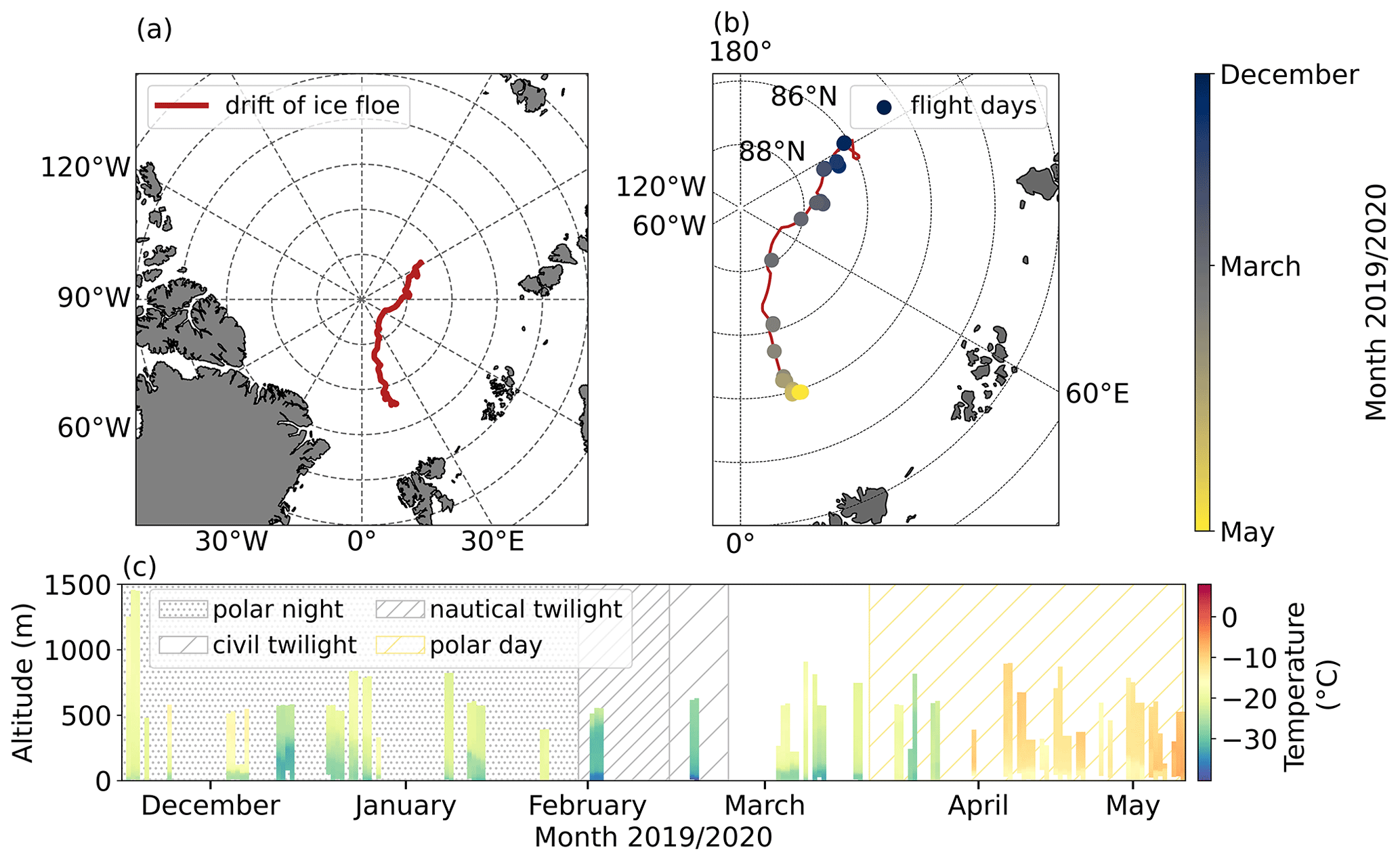
Figure 1 Overview of the drift of the ice floe during tethered balloon operations in winter and spring (a), as well as daylight conditions and location of the days with balloon operations (b). Temperature measurements of all profiles are shown in (c). The background shading indicates the respective daylight conditions during the observation period, with the white background indicating the period with a diurnal cycle.

Another approach to define the SML height applies the bulk Richardson number Ri_b (Andreas et al., 2000; Zilitinkevich and Baklanov, 2002; Dai et al., 2014; Zhang et al., 2014; Jozef et al., 2022; Peng et al., 2023). Ri_b is derived from the ratio between shear and buoyancy and is a measure of the likelihood of turbulence. Ri_b below the critical value indicates an atmospheric layer that is likely to remain or become turbulent. Turbulence cannot be sustained, and laminar layers will not become turbulent if the Ri_b is above a critical value. The SML height is defined by the height where turbulence cannot be sustained because the Ri_b exceeds a critical value of Ri_b (Zilitinkevich and Baklanov, 2002; Andreas et al., 2000). This critical value, however, is under discussion and varies, for example, among sites (Vickers and Mahrt, 2004).

We use the turbulence-based SML heights as a reference to derive a critical Ri_b for the winter and spring. The in situ turbulence perspective allows us to not only derive a critical value but also to evaluate the Ri_b approach. It should be emphasized that this approach can also be applied to a stably stratified atmosphere. Further continuous, surface-based energy flux measurements can be used to estimate the SML height using Monin–Obukhov similarity theory (Zilitinkevich, 1972; Vickers and Mahrt, 2004). The Monin–Obukhov similarity theory describes the near-surface turbulent exchange processes based on surface measurements. This approach can complement the balloon-borne SML height estimates between balloon launches.

The current study discusses observed profile measurements of Arctic ABL turbulent properties and related effects of clouds on the vertical thermodynamic structure. The data are used to develop a new, more accurate approach to estimate the SML height in Arctic winter and spring. To investigate possible SML height criteria, the in situ energy dissipation rates are compared to Ri_b profiles and a surface-flux-based method. Furthermore, we apply the critical Ri_b value technique for deriving the SML height using both tethered balloon and radiosonde data.

2 Data and methods

2.1 Observations in winter and spring during the MOSAiC expedition

During the MOSAiC expedition, the research vessel (RV) Polarstern (Knust, 2017) was frozen to an ice floe drifting from October 2019 until September 2020. The MOSAiC expedition facilitated measurements on board RV Polarstern and on the ice floe covering the atmosphere, Arctic Ocean, sea ice, ecosystem, and biogeochemistry throughout an entire seasonal cycle. An overview of the atmospheric measurements is given by Shupe et al. (2022), and information about the sea ice and oceanographic aspects is summarized by Nicolaus et al. (2022) and Rabe et al. (2022). Figure 1a shows the course of the drift of RV Polarstern in winter and spring when the tethered balloon Miss Piggy (Becker et al., 2020) was deployed from the ice floe close to RV Polarstern. A detailed view of the temporal evolution and the balloon flight days is given in Fig. 1b. The balloon was filled with helium, has a volume of about 9 m³, and allows lifting a modular scientific payload of up to 4 kg. The tethered balloon enables continuous vertical profiling of the lowermost 1.5 km of the atmosphere with a climbing rate of around 1 m s⁻¹. Measurements can be performed day and night as well as under cloudy conditions with light icing. The deployment of the balloon is inhibited by strong winds (wind velocity above about 7 m s⁻¹ at the surface) or precipitation associated with severe icing. Therefore, weather-related selective sampling should be considered for further interpretation.

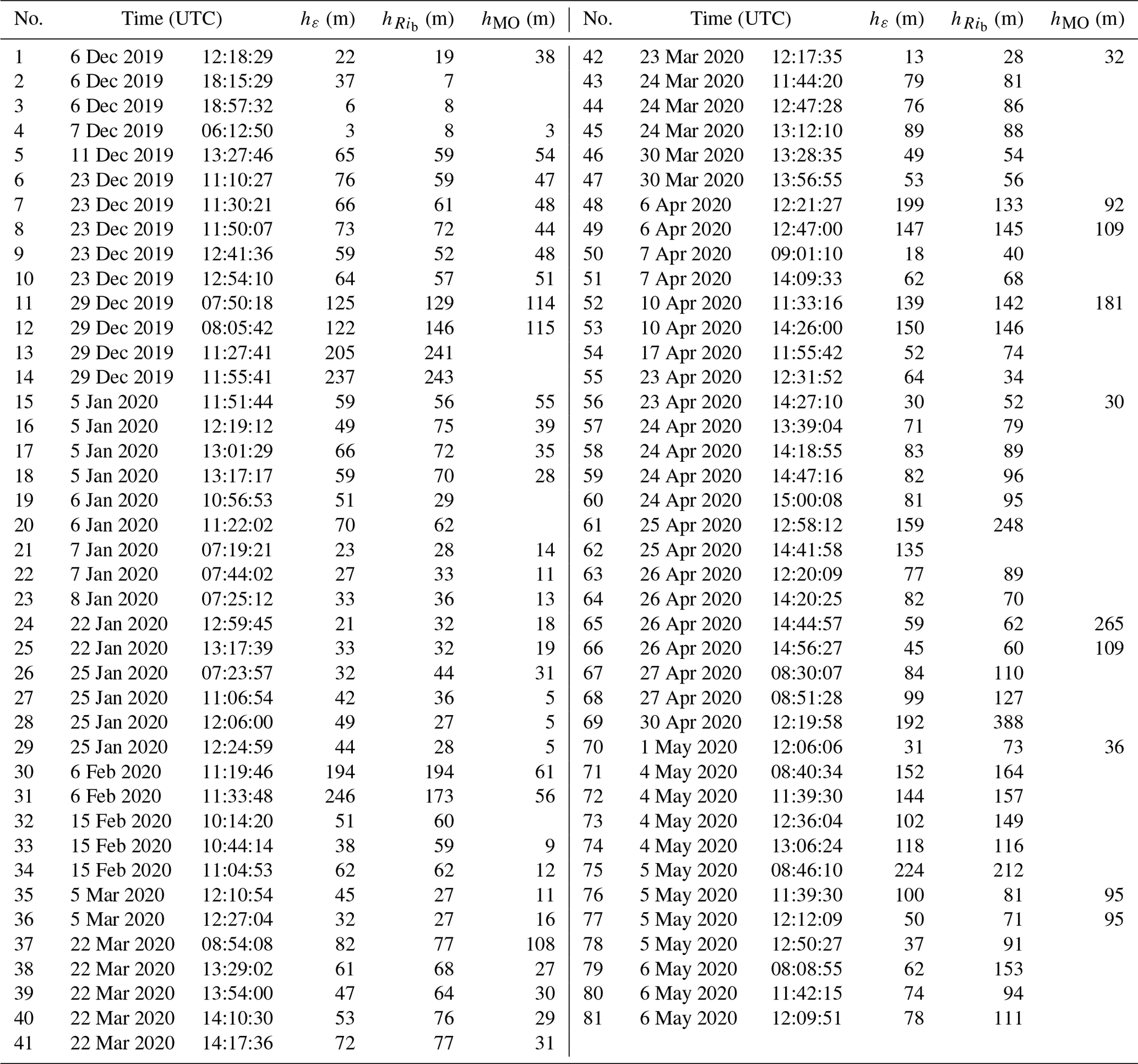
A hot-wire anemometer package specifically designed for turbulence observations (Egerer et al., 2019), hereafter referred to as the “turbulence probe”, was used to measure the data for this study. Data were collected when the ice floe drifted between 86.14^∘ N, 122.21^∘ E and 83.92^∘ N, 17.69^∘ E between 6 December 2019 and 6 May 2020 (Fig. 1b). The entire dataset and its processing are described by Akansu et al. (2023b). The instrument is attached to a tether about 10 to 20 m below the balloon to minimize flow distortions induced by the balloon. In addition, the instrument package attached to the balloon tether is mounted flexibly; it is aligned horizontally and equipped with a tail to keep the setup in the mean flow direction. The instrument consists of a hot-wire anemometer to measure wind velocity with 125 Hz temporal resolution and a thermocouple for air temperature measurements with 10 Hz temporal resolution. Besides the high-frequency records, 1 Hz measurements of wind velocity based on a Pitot static tube have been made, along with basic measurements of static pressure, temperature, and relative air humidity. Due to weather conditions, the Pitot tube, which served as a reference for hot-wire calibration, was frequently affected by icing. Therefore, a standard meteorology tethersonde, which belongs to the modular balloon equipment and is separated about 10 m from the turbulence probe, was the mean reference for the fast sensors. The turbulence probe was deployed on 34 d, sampling the height range from the surface to typically a few hundred meters. After quality control, 99 individual vertical profiles (ascents and descents) have been provided for further analysis. In this study, 81 out of the 99 profiles are used because not all measurements reach the surface, and some contain error-prone temperature data. Figure 1c displays an overview of all temperature profiles, the respective maximum height, and daylight conditions. Table A1 shows all profiles and their launch times.

Continuous, near-surface observations of meteorological and turbulence parameters were performed at a location on the ice floe called Met City (Shupe et al., 2022). There was about 300 m of distance between Met City and the balloon operation site, increasing over time due to ice flow dynamics. Measurements with an ultrasonic anemometer and thermometer were taken at a meteorological tower at 2, 6, and 10 m heights, serving as a surface reference for our balloon observations. Furthermore, the upward (^↑) and downward (^↓) broadband terrestrial irradiances F (in units of W m⁻²) were collected at the atmospheric surface flux station with a precision infrared radiometer (Shupe et al., 2022). The net terrestrial irradiances F_net = F^↓ − F^↑ are taken as a proxy for the radiative energy budget at the surface. Furthermore, the measurements at Met City include the surface radiometric skin temperature.

Regular radiosondes were launched every 6 h (05:00, 11:00, 17:00, and 23:00 UTC) from the helicopter deck of RV Polarstern (12 m above mean sea level), providing information on the dynamic and thermodynamic structure of the atmosphere. It should be noted that the data obtained within the first tens of meters can be influenced by the ship itself and should therefore be interpreted with caution. The ship can create flow distortions and can serve as a heat island, but radiosonde data near the surface are also often still subject to errors. The wind determined by GPS (Global Positioning System) data in particular might be influenced by the unwinding of the probe from the tether (Achtert et al., 2015; Jozef et al., 2022). To compare the radiosonde and the tethered balloon profile measurements, the corresponding radiosonde data are selected with launch times closest to the tethered balloon flight. The time difference between the two launches is, at most, around 3 h, in which the SML height typically did not change significantly, as shown by Jozef et al. (2022). However, the atmospheric structure may change within a few hours or even less.

The Arctic ABL can be very shallow, especially in winter and during cloudless conditions. However, the cloudy Arctic ABL is also often shallow and hence poses challenges for remote sensing approaches to detect the very low cloud layers (Griesche et al., 2020). For the question of the influence of clouds on the ABL dynamics, however, the net irradiances are of main importance, which are directly influenced by the clouds. Therefore, F_net measurements at Met City, where F_net is the cumulative surface irradiance, are used as an independent “cloud indicator”. F_net can be used to distinguish between cloudless and cloudy conditions during both polar day and night. Cloudless conditions prevail when the net radiation is below −25 W m⁻², while higher values are associated with clouds (Wendisch et al., 2023a). To avoid ambiguous allocations, data with net radiation in the range between −28 and −22 W m⁻² are not considered. Additionally, the cloud condition was manually compared with 360^∘ photographs and total-sky imager observations (as far as possible regarding daylight conditions).

2.2 Estimation of the surface mixing layer height

In this section, we present several methods for determining SML heights based on different available datasets. First, we discuss a method to derive SML heights that directly benefits from local turbulence measurements and will serve as a reference for other approaches in the following (Sect. 2.2.1). A second method is based on the mean temperature and wind speed profiles in the context of the Ri_b criterion (Sect. 2.2.2). Finally, we compare the previous results with SML heights based on the application of the Monin–Obukhov similarity theory and thus on the determination of surface fluxes (Sect. 2.2.3).

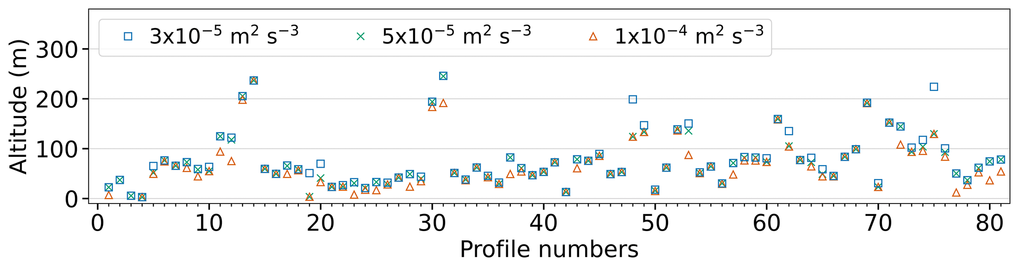
Figure 2 Surface mixing layer heights derived from direct turbulence measurements for each profile. Three thresholds separate turbulent and non-turbulent flows: 1 × 10⁻⁴, 5 × 10⁻⁵, and 3 × 10⁻⁵ m² s⁻³.

2.2.1 Direct in situ method

The direct in situ method for estimating the SML is based on the assumption that the turbulence at the top of this layer falls below a certain threshold, indicating the transition from a turbulent to a comparatively laminar layer. For our application, we chose the energy dissipation rate ε to quantify turbulence because it can be determined as a local parameter from short temporal subsections during a balloon ascent. Based on Kolmogorov's inertial subrange theory, ε can be estimated in different ways (Wyngaard, 2012). A comparatively robust and proven method has been found to determine ε using the second-order structure function (Siebert et al., 2006):

$$\begin{array}{}\text{(1)}& S^{\left(\mathrm{2}\right)}\left(\mathit{\tau }\right)=〈\left(u\right(t+\mathit{\tau })-u(t){)}^{\mathrm{2}}〉=\mathrm{2}(\mathit{\epsilon }\cdot U\cdot \mathit{\tau }{)}^{\mathrm{2}/\mathrm{3}},\end{array}$$

with u(t) the longitudinal wind velocity component as measured at time t. The averaging in Eq. (1) denoted by the angle brackets is performed over all t, so the structure function S⁽²⁾ is a function of time lag τ, which has been calculated by applying Taylor's frozen turbulence hypothesis (transferring the time lag to spatial increment $r=U\cdot \mathit{\tau }$) with the mean flow velocity U (see Stull, 1988, for more details). It has been shown by Frehlich et al. (2003) that 100 samples are sufficient in order to provide robust estimates of local ε. Here, we use an integration over 125 samples (e.g., 1 s), resulting in a vertical resolution of roughly 1 to 2 m.

Profiles of ε allow direct identification of the SML height, denoted hereafter as h_ε. This method has the disadvantage that there is no physically unambiguous definition of the limit value for ε, and therefore different values are used in the literature (Shupe et al., 2013; Brooks et al., 2017), which are close to each other. We tested three values to estimate h_ε that have been used previously: 1 × 10⁻⁴, 5 × 10⁻⁵, and 3 × 10⁻⁵ m² s⁻³. We consider the SML to be constrained when ε falls below the threshold for at least 10 consecutive levels, while h_ε equals the lowermost of those levels. These 10 levels ensure that the turbulent layer and non-turbulent layer are well separated.

Figure 2 shows the estimates of h_ε for each profile for the different thresholds. The profile numbers refer to the profiles used in this study. An overview is given in Table A1. The highest threshold almost always yields the lowest h_ε values, and the two lowest thresholds are very close and result in nearly identical values of h_ε. To identify the appropriate threshold value, we have compared the SML heights derived by different thresholds with the potential temperature profiles. Additionally, we have examined whether the SML height coincides with a significant change in ε. As a result we have decided on the threshold value of ε = 3 × 10⁻⁵ m² s⁻³.

2.2.2 Bulk Richardson number method

The turbulent state of an atmospheric layer can be analyzed using the (gradient) Richardson number Ri_g, which describes the relationship between thermodynamic stability and turbulence-producing horizontal wind shear (e.g., Stull, 1988):

$$\begin{array}{}\text{(2)}& R{i}_{\mathrm{g}}\left(z\right)={\displaystyle \frac{\frac{g}{\mathit{\theta }}\frac{\partial \mathit{\theta }}{\partial z}}{{\left(\frac{\partial u}{\partial z}\right)}^{\mathrm{2}}+{\left(\frac{\partial v^{\mathrm{2}}}{\partial z}\right)}^{\mathrm{2}}}},\end{array}$$

with the potential temperature of dry air θ, the horizontal wind components u and v (zonal and meridional), the gravitational acceleration g = 9.81 m s⁻², and z as height above ground. This stability measure describes whether there is a tendency for turbulence to weaken or strengthen. Ri_g smaller than the theoretical value of 0.25 refers to a turbulent atmospheric layer. Therefore, Ri_g profiles can be used to derive the equilibrium height at which turbulence decays, which coincides with the SML height $h_{R{i}_{\mathrm{g}}}$ (Zilitinkevich and Baklanov, 2002; Andreas et al., 2000). However, the practical use of Ri_g is somewhat limited because the calculation of (local) wind and temperature gradients based on observational data is often subject to uncertainties that lead to large scatter in the Ri_g profiles. In particular, the necessary filtering leads to further ambiguities. For this reason, modified definitions for Ri_g have been derived, which offer advantages, especially for observational data. An alternative Ri number is the so-called surface bulk Richardson number Ri_b (Mahrt, 1981; Andreas et al., 2000; Heinemann and Rose, 1990), whose definition is not based on the explicit calculation of local gradients but includes the complete layer from the surface to the current measurement height z:

$$\begin{array}{}\text{(3)}& R{i}_{\mathrm{b}}\left(z\right)={\displaystyle \frac{g\cdot z\cdot \frac{\mathrm{\Delta }\mathit{\theta }}{{\mathit{\theta }}_{\mathrm{0}}}}{U(z{)}^{\mathrm{2}}}},\end{array}$$

where θ₀ is the potential temperature of dry air at the surface and $\mathrm{\Delta }\mathit{\theta }=\mathit{\theta }\left(z\right)-{\mathit{\theta }}_{\mathrm{0}}$ is the temperature difference between the surface and z. According to the basic concept of the surface bulk Richardson number approach, the lower reference level is the surface where the mean horizontal wind velocity equals zero U(z=z₀) and θ₀ is the skin temperature. In the following, Ri_b always refers to the surface bulk Richardson number. Since other studies are often based on radiosonde observations only, the temperature at 2 m is then typically used for θ₀, even though this value may differ from the skin temperature, especially for stably stratified conditions with strong surface temperature gradients. To be consistent with other studies, we first use temperature observations at 2 m from the Met City tower for θ₀. Then, for comparison, the same analysis is performed using the skin temperature measured during MOSAiC.

Compared to other bulk Ri definitions, where mean gradients are estimated for distinct layers of δz = 30 m (Jozef et al., 2022), for example, the Ri_b approach applied here fails if multiple turbulent layers are present. However, as we want to estimate the height of the SML, only the lowermost continuous turbulent layer needs to be detected, and the surface approach with an increasing layer depth is sufficient. Furthermore, from the values of h_ε presented in Fig. 2, it becomes apparent that the majority of the SML heights lie within the lowermost 100 m; many even do not exceed 50 m altitude and multiple turbulence layers are rare.

The height of the SML $h_{R{i}_{\mathrm{b}}}$ is the height at which Ri_b reaches a critical value and the turbulence decays. The top of the SML is thus the highest level where Ri_b < Ri_bc. However, the definition of Ri_bc is not straightforward and not based on a theoretical concept. It appears that the differences for Ri_bc measured at different sites are larger than the variation within an observation period at a fixed site (Vickers and Mahrt, 2004). When applying 0.25 as a critical value for the bulk approach, the experimentally determined SML heights are overestimated (Brooks et al., 2017). However, this theoretical critical value was derived for the gradient Ri_g number and is therefore not directly applicable to the surface bulk approach. In addition, Eq. (3) is sensitive to the lowest observation level, which may also explain some of the variation in Ri_bc. However, using the “reference” SML height h_ε introduced in Sect. 2.2.1, we can provide a direct and robust estimate for Ri_bc (see Sect. 3.3).

2.2.3 Surface-flux-based method

If surface energy fluxes are the main drivers for the development of an SML, it is proposed that the SML height is a function of the Monin–Obukhov length L (Vickers and Mahrt, 2004):

$$\begin{array}{}\text{(4)}& L=-{\displaystyle \frac{u_{\star }^{\mathrm{3}}}{B_{\mathrm{s}}}},\end{array}$$

with $B_{\mathrm{s}}=g\cdot {T_{\mathrm{0}}}^{-\mathrm{1}}〈w^{\prime }\cdot T^{\prime }〉$ being the surface buoyancy flux and $u_{\star }^{\mathrm{2}}=-〈u^{\prime }\cdot w^{\prime }〉$ being the friction velocity. Besides more simple relationships (e.g., h∝L, Kitaigorodskii, 1960), Zilitinkevich (1972) proposed a formulation including the Earth's rotation:

$$\begin{array}{}\text{(5)}& h_{\text{MO}}=C\sqrt{{\displaystyle \frac{u_{\star }L}{f}}},\end{array}$$

with C being a scaling constant of 𝒪(1) and the Coriolis parameter f. All parameters included in Eq. (5) were calculated continuously using ultrasonic anemometer readings at the Met City tower. With the Monin–Obukhov scaling method, referred to as the MO method hereafter, the SML height can be derived continuously and complements balloon-borne SML height estimates. However, Eq. (5) is only valid for stable stratification (B_s<0 and L>0), and the method fails if further sources of turbulence are present at higher levels (such as clouds or low-level jets – LLJs). Again, the in situ turbulence method is helpful to assess the applicability of the MO method (Sect. 3.5).

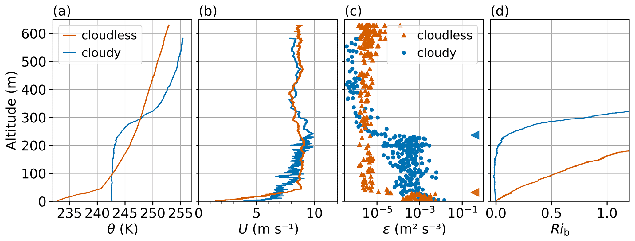
Figure 3 Tethered balloon-borne profiles obtained under cloudless conditions (orange) on 5 March 2020 at 12:27 UTC and under cloudy conditions (blue) on 29 December 2019 at 11:55 UTC. Panel (a) shows the profiles of potential temperature over height, (b) the wind velocity, (c) the derived energy dissipation rates, and (d) the surface bulk Richardson number. The SML heights for cloudless (orange) and cloudy conditions (blue) derived by in situ turbulence records are indicated by left-pointing triangles on the right in (c).

3 Results and discussion

3.1 Surface-based versus elevated inversion

In the Introduction, we have argued that the Arctic winter ABL mainly alternates between cloudless and cloudy conditions. We begin at this point by illustrating these two typical conditions, presenting two examples. The first case represents a cloudless ABL with a pronounced surface inversion, and the second case describes a cloudy ABL and the resulting elevated inversion at the cloud top with a well-mixed layer below the inversion. Figure 3 shows the two example measurements of potential temperature θ, horizontal wind velocity U, local energy dissipation rate ε, and surface bulk Richardson number Ri_b as a function of altitude. Cloudless conditions prevailed during a profile observed on 5 March 2020 with a strong surface-based temperature inversion (Δθ≈ 7 K within about 40 m) up to 50 m followed by a less stably stratified layer above (Fig. 3a). The wind velocity U increases with height from the surface up to a height of about 50 m and then remains almost constant up to the maximum height of the profile (Fig. 3b). The strongest increase in U is in the lowest altitude layers up to about 30 m, the region with the highest turbulence in terms of ε (Fig. 3c). Above 30 m, the turbulence decreases rapidly by 2 to 3 orders of magnitude, and according to the threshold, as defined in Sect. 2.2.1, the upper limit of the SML height is reached here. The Ri_b (Fig. 3d) increases almost linearly with height for the cloudless conditions.

The example for the vertical stratification under cloudy conditions, as measured on 29 December 2019, shows an elevated inversion with its base at around 220 m. A well-mixed layer prevails below the inversion, with U gradually increasing from the surface to the inversion base from 6 to 9 m s⁻¹. Clearly, the turbulence reaches from the surface up to about 240 m height, where ε rapidly drops below the threshold, indicating the SML height. The extent of the SML is also clearly visible in the Ri_b profile (Fig. 3d). The Ri_b remains almost constant with height in this region with values close to zero; it starts to increase significantly only at the inversion base height, exactly where ε starts to decrease quite abruptly and the upper limit of the SML height is reached.

3.2 Vertical mean and turbulent structure of the ABL

To illustrate the main features of the mean temperature stratification for the two typical situations, we normalize, plot, and average all measured profiles (Fig. 4), distinguishing between surface (Fig. 4a) and elevated (Fig. 4b) inversions. The height is normalized by h_ε, and the temperature is shifted by the surface value θ₀ and normalized by the inversion strength $[\mathrm{\Delta }\mathit{\theta }=\mathit{\theta }(h_{\mathit{\epsilon }})-{\mathit{\theta }}_{\mathrm{0}}]$ so that the normalized temperature in the SML height takes the value 1. A similar plot, including the contrasting summertime Arctic, can be found in Tjernström and Graversen (2009).

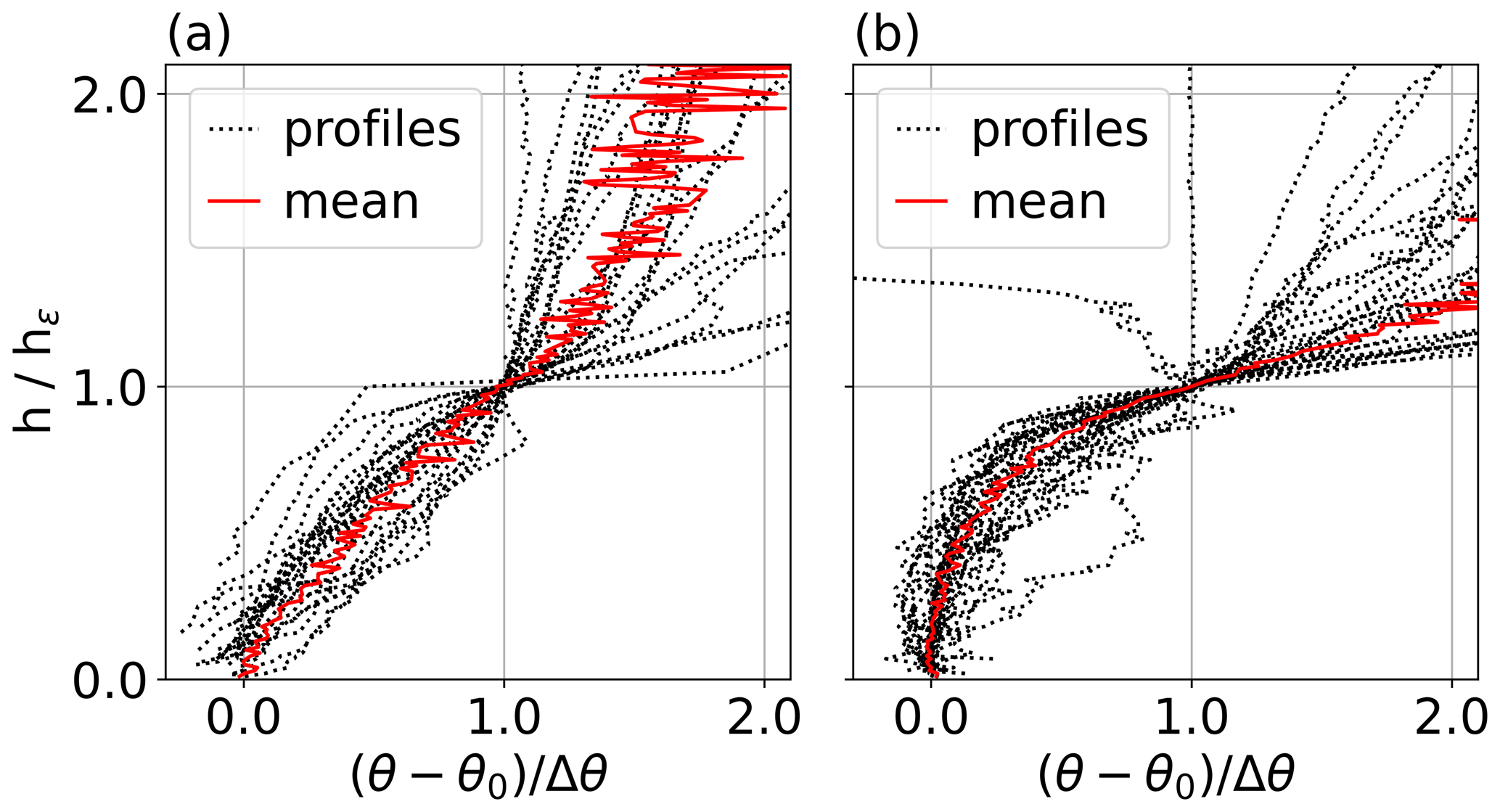
Figure 4 Normalized potential temperature profiles of tethered balloon-borne measurements over height. All profiles are separated with respect to the inversion heights, such as surface-based inversion (a) or elevated inversion (b). The height is normalized using the turbulence-based SML height h_ε, while the temperature is normalized using the potential temperature gradient of the SML and the potential temperature close to the surface.

Due to operational constraints, not all profiles reach the same height, but all launches used here exceed 200 m altitude, and therefore most profiles exceed at least twice the h_ε. The two averaged temperature profiles have quite different characteristics. While the profile is nearly linear from the surface to h_ε for cloudless conditions, the well-mixed sub-cloud layer for the cloudy case shows a gradual increase in temperature, rising much more sharply at h_ε. As is often observed in Arctic clouds, the temperature increase at the inversion base already begins inside the cloud; this normalization does not consider the cloud layer thickness, and hence the temperature curve in Fig. 4b must be interpreted with caution. In addition, it must be emphasized that we do not present the equivalent potential temperature, which under adiabatic conditions is also height-constant within the cloud.

Figure 5 shows the relative probability distribution of ε using 5 m height intervals of all measured profiles. The turbulence distribution for surface-based inversions (Fig. 5a, 30 profiles) shows the highest values near the surface (wind-shear-driven turbulence) and significantly lower ones above approximately 60 m height. Higher probabilities of ε at around 500 m height occurred during single events and might be related to LLJs. However, the observations are too sparse to draw conclusions about the occurrence of possible multi-layer turbulent structures. For ABL structures with elevated inversions (Fig. 5b, 34 profiles), the turbulence is still highest in the lowermost tens of meters. But here, the turbulence reaches up to around 200 m. The chosen threshold of ε = 3 × 10⁻⁵ m² s⁻³ distinguishes turbulent and non-turbulent regions of the profiles. With this threshold approach, almost all observations above 300 m height for elevated inversions (60 m height for surface inversions) are considered non-turbulent and thus well above the SML. In contrast to the summertime Arctic ABL, where Brooks et al. (2017) found two separated turbulence maxima indicating decoupling, we did not identify clearly pronounced turbulence layering, and decoupling plays a minor role.

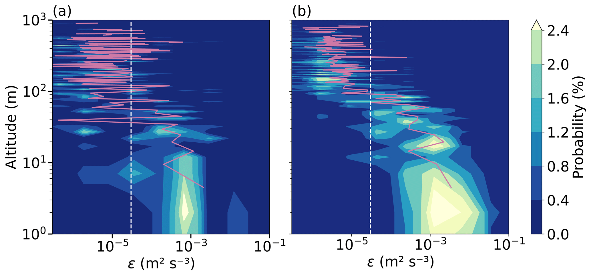
Figure 5 Probability of the energy dissipation rates as a function of height. The profiles are distinguished with respect to the temperature profile: panel (a) shows all profiles with surface-based inversions and (b) profiles with elevated inversions. The probability of ε is calculated for 5 m height bins starting at a height of 2 m. To complement the data from the surface, the first bin reaches from the surface up to a height of 2 m. Additionally, the median (solid line) profile of ε (5 m bins starting at 2 m height) is given in purple. The turbulence threshold value of 3 × 10⁻⁵ m² s⁻³ is depicted by the dashed white vertical line in both panels.

3.3 Estimating the critical bulk Richardson number

Estimating the SML height based on the Ri_b requires a critical value Ri_bc. Here, we apply a method used by Vickers and Mahrt (2004) by plotting the buoyancy term against the shear term for all profiles at h_ε in Fig. 6. The slope of the linear fit corresponds to the critical surface bulk Richardson number Ri_bc. Based on data from 80 profiles, we derive a critical value of Ri_bc = 0.12, about half the theoretical value of 0.25. As mentioned in Sect. 2.2.2, we would like to point out again that this “theoretical value” should be understood as an order of magnitude for the Ri_b approach rather than a reference value. Applying the same analysis with the skin temperature as θ₀, we derive Ri_bc = 0.16 (Fig. 6). This difference clearly shows how strongly the derived value for Ri_bc depends on the selected surface reference. Furthermore, we can assume that the temperature measured at a height of 2 m on a mast is also significantly more accurate than a corresponding measurement with a radiosonde, which has comparatively large inaccuracies in the lower ranges.

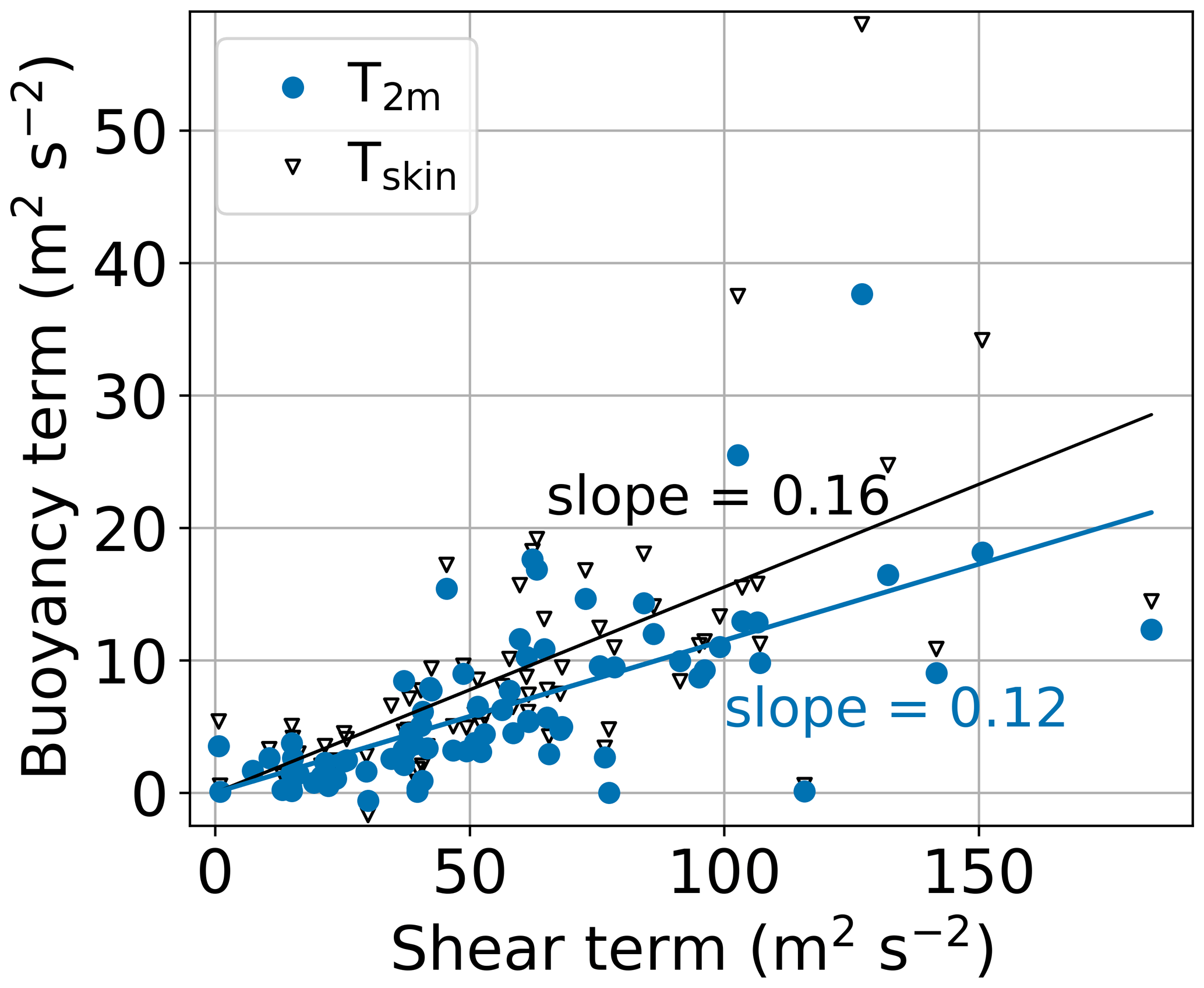
Figure 6 The buoyancy term versus shear term of the surface bulk Richardson number calculated according to Eq. (3) using the temperature at 2 m height T_2 m (blue) and the skin temperature T_skin (black) as θ₀. The solid line indicates the least-squares fit that is forced through the origin. The critical bulk Richardson number Ri_bc is equivalent to the slope of the fit. The critical values are 0.12 for T_2 m and 0.16 for T_skin.

To obtain a rough measure of the robustness of the Ri_bc estimate, Fig. 7 shows the frequency of occurrence of Ri_bc. Clearly, the majority of Ri_bc values using the temperature at 2 m height as θ₀ are centered around the critical value of 0.12, with a few outliers exceeding this value. The frequency distribution of Ri_bc with T_skin as θ₀ is slightly shifted towards higher Ri_bc values.

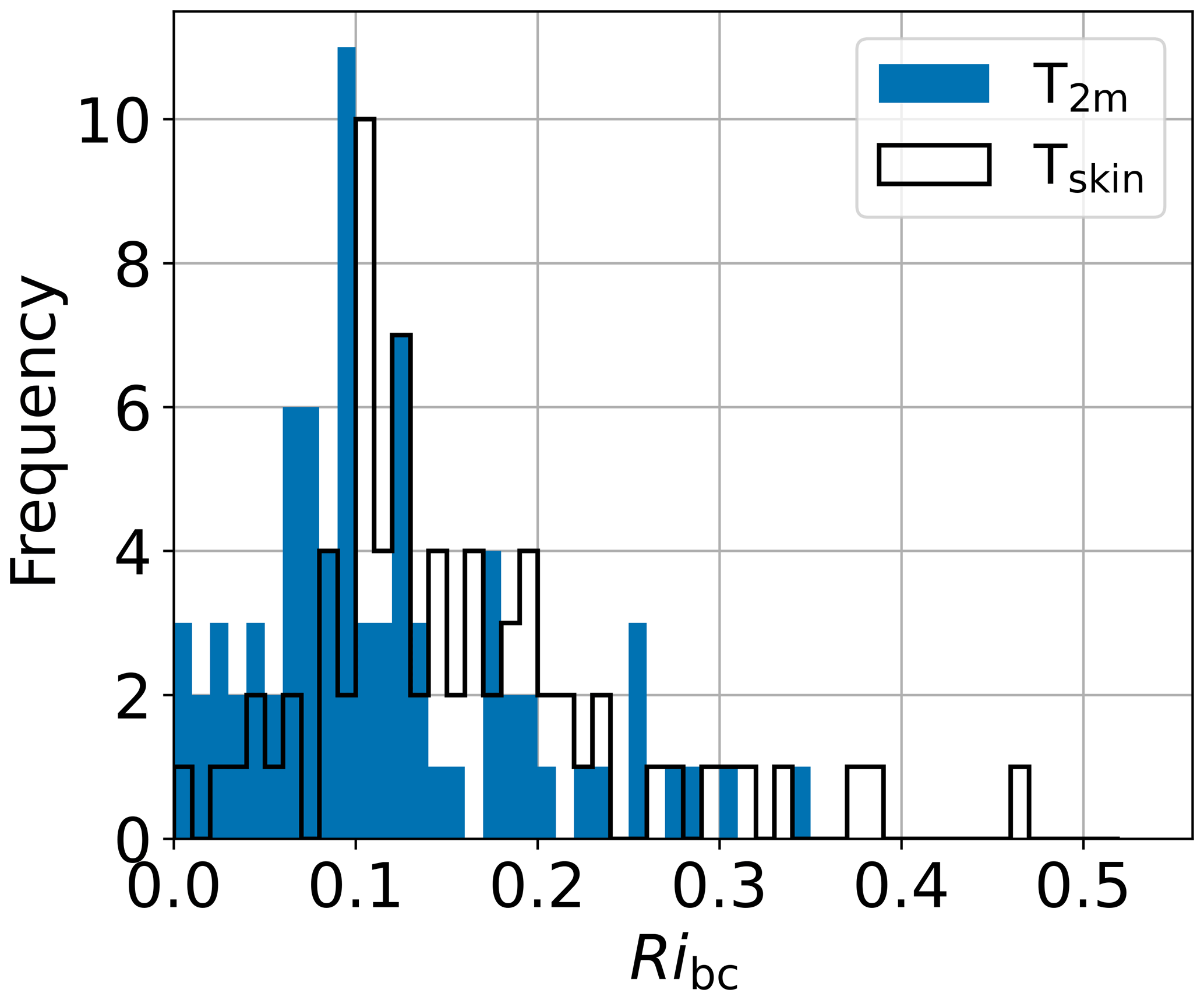
Figure 7 Frequency distributions of surface bulk Richardson numbers at the SML height h_ε using the temperature at 2 m height T_2 m (blue) and the skin temperature T_skin (black) as θ₀.

As described by Vickers and Mahrt (2004), the Ri_bc not only varies between sites but is also a function of atmospheric conditions (cloudless, cloudy). To understand which influence may lead to different values of Ri_bc, we distinguished the data by the cloud conditions using F_net. While we have derived Ri_bc for cloudless and cloudy conditions, the differences between the two typical ABL types are negligible. The critical value of Ri_bc = 0.12 can be used for all conditions (with temperature measurements at 2 m height as θ₀).

3.4 Surface mixing layer height estimates based on a mean critical Richardson number

To assess the impact of using an averaged critical Ri_b number on the individual SML height, we compare $h_{R{i}_{\mathrm{b}}}$ to the turbulence-based value h_ε. In addition to the tethered balloon profiles, we apply the same Ri_b method to the radiosondes profiles using the Met City tower data as a surface reference. Figure 8 shows the comparison of the SML heights applying two different Ri_bc values for both tethered balloon-borne and radiosonde profiles. We use radiosonde profiles launched closest to the tethered balloon flight.

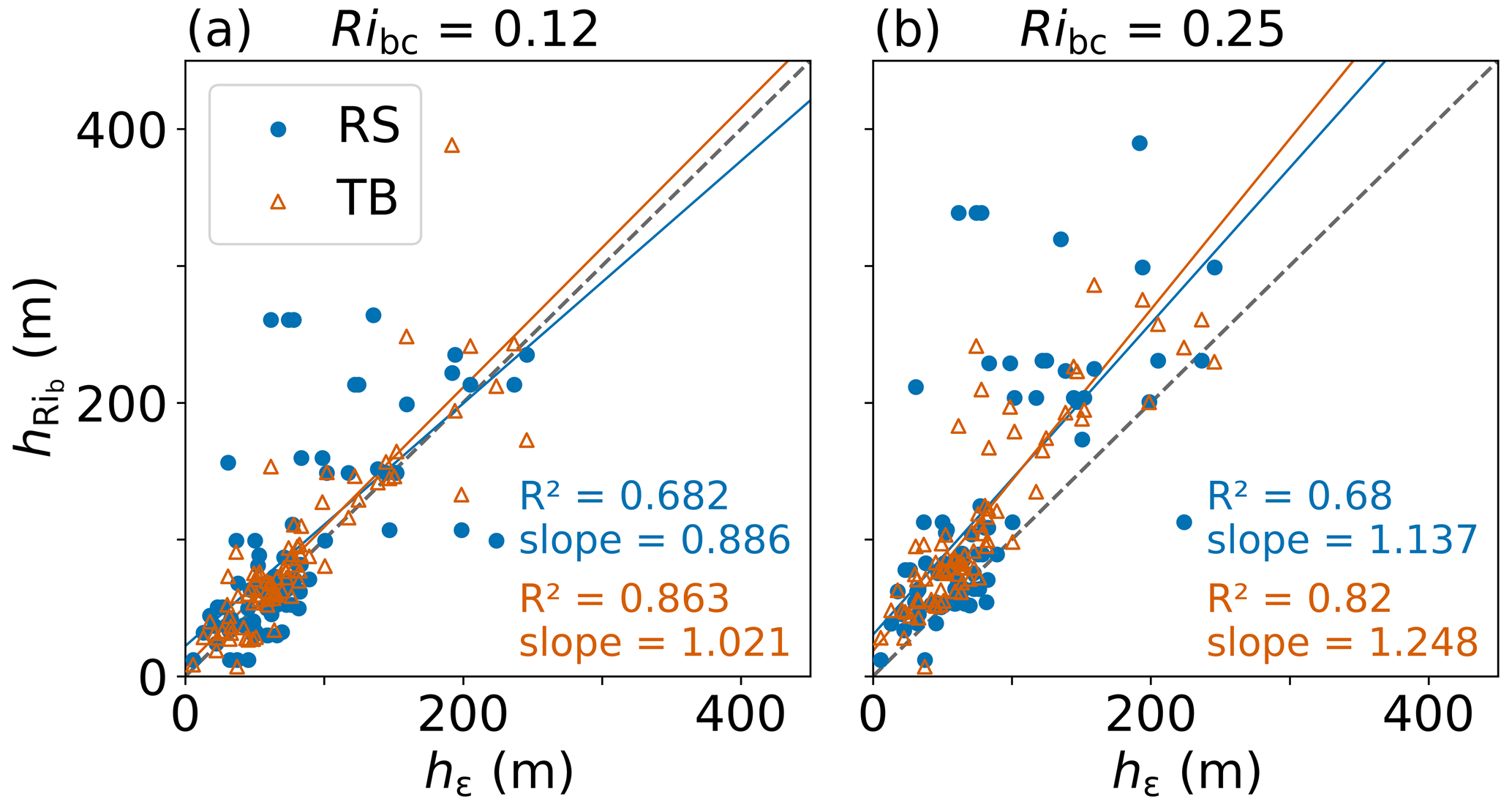
Figure 8 SML height comparisons between the Ri_b approach $h_{R{i}_{\mathrm{b}}}$ and turbulence h_ε based on tethered balloon (TB, orange) and radiosonde (RS, blue) profiles. For both datasets, two different critical Ri_b values are used: 0.12 (a) and 0.25 (b). The dashed line represents the 1:1 line. Solid lines are the least-squares fits for tethered balloon (orange) and radiosonde (blue) profiles; R² and slope values are given for each fit.

For the tethered balloon observations, the slope using the theoretical value of 0.25 is about 22 % higher than when using Ri_bc=0.12. As all intercepts are positive, a slope > 1 indicates an overestimation of h. Compared to h_ε, $h_{R{i}_{\mathrm{b}}}$ with Ri_bc=0.12 is about 15 % higher, while Ri_bc=0.25 leads to about a 60 % overestimation of h. This supports the need for an accurate estimate of Ri_bc. If we apply the newly determined Ri_bc and the theoretical value for comparison to the radiosonde observations, the inaccuracies in h become even more apparent. Besides the slope, the intercept also increases (from 22 with Ri_bc=0.12 to 30 with Ri_bc=0.25), leading to an overestimation of h. It should be noted that the reference height h_ε was not determined at the same time as the height based on the radiosonde ascents, which may explain some of the observed differences.

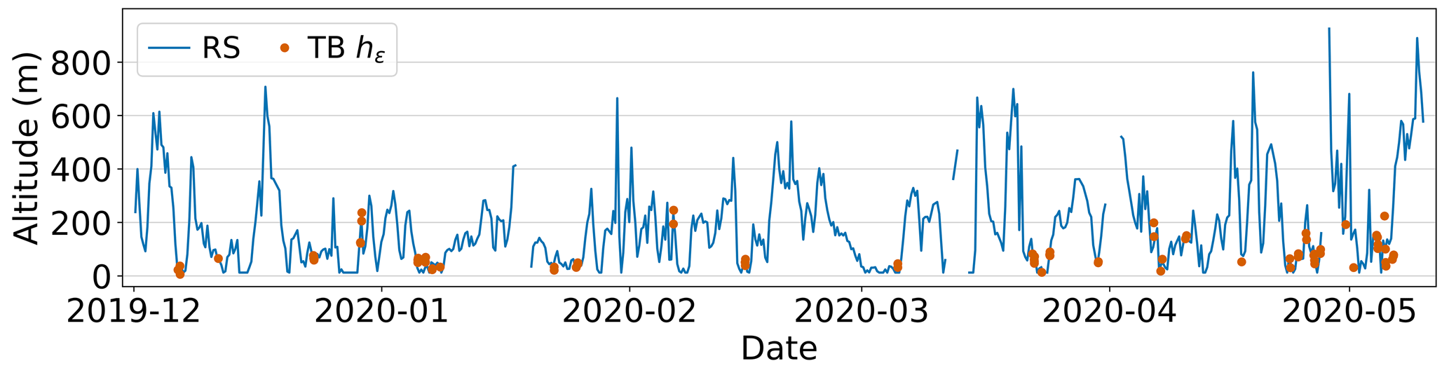
Figure 9 Time series of SML heights from radiosonde data derived with the surface bulk Richardson number method using Ri_bc = 0.12. The time series of radiosonde launches is displayed between 1 December 2019 and 10 May 2020 (blue). Additionally, the SML heights h_ε of tethered balloon-borne profiles are shown as orange dots.

Furthermore, we use Ri_bc=0.12 to derive h for all radiosonde launches collected during winter and spring. Figure 9 shows the time series of the derived SML height and additionally h_ε of the tethered balloon-borne turbulence estimates. In Fig. 9, a high variability of the SML height is displayed during the entire observation period, reaching from a few tens of meters up to 600 m or more (maximum 925 m). It has to be considered that the minimum detection limit of the radiosonde is of about 12 m due to launching from the helicopter deck. Significant growth of the SML is likely related to weather or storm events, while the SML is shallower for calm or stable conditions. The vast majority (around 81 %) of the SML heights derived from the radiosondes during this period are below 300 m, and around half of the profiles contained an SML with height lower than 150 m. The tethered balloon operations primarily cover periods of lower wind velocities and shallower SML heights, and during storm events the SML can be much deeper. Whether Ri_bc may change during these events remains open and cannot be answered in this study.

Frequency distributions of all derived SML heights using radiosonde data are shown in Fig. 10. During the period considered in this plot, the majority of the SML heights are below 250 m (Fig. 10a). Separating between cloudless and cloudy conditions shows that SML heights are spread rather equally for cloudy conditions but are significantly lower for cloudless conditions (Fig. 10b). During daylight conditions (Fig. 10c and d), the lowest SML heights are measured under cloudless conditions. However, the number of daylight profiles is lower than the number of night profiles for our analysis period. Distributions of the SML heights during polar night are shown in Fig. 10e for all conditions and separated by cloud conditions in Fig. 10f. We see that the majority of cloudless conditions lead to SML heights of a maximum of 100 to 200 m, while cloudy conditions do not show any tendency towards a distinct SML height. This distribution shows the variety of clouds and their respective influence on the SML. Furthermore, the wind velocity can play a role in the variation of the SML heights as the wind velocity can vary significantly during cloudy conditions.

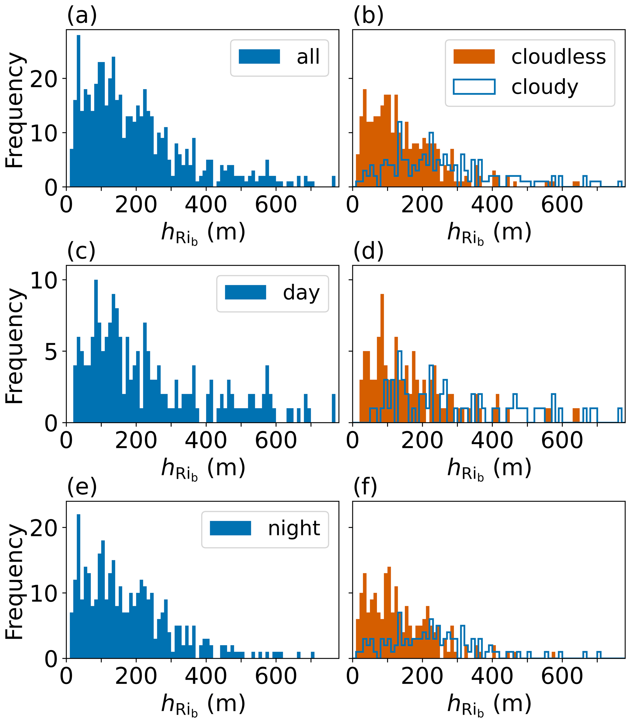
Figure 10 Frequency distribution of SML heights using radiosonde data between 1 December 2019 and 10 May 2020. The radiosonde SML heights are based on the Ri_b approach with Ri_bc = 0.12. The frequency distributions are given for (a) all radiosonde profiles, (b) all data separated according to cloud conditions, (c) all profiles with daylight conditions, and (e) all profiles during night; panels (d) and (f) show the cloudless and cloudy conditions in orange and blue, respectively.

3.5 Surface mixing layer height estimates based on Monin–Obukhov scaling

Under stable conditions (B_s<0 and L>0), we apply the surface-flux-based method introduced in Sect. 2.2.3 to determine the SML height h_MO based on Monin–Obukhov scaling. The two covariances underlying the definition of L are estimated from ultrasonic anemometer and thermometer observations from the Met City tower at 2 m height. A running average ($\stackrel{\mathrm{̃}}{x}\left(t\right)$) with a centered window over 5 min is applied to define the time series of the fluctuating part as $x^{\prime }\left(t\right)=x\left(t\right)-\stackrel{\mathrm{̃}}{x}\left(t\right)$, where $〈x^{\prime }\left(t\right)〉=\mathrm{0}$ is fulfilled and x is one of the velocity components ($u,v,w$) or virtual temperature T_v (actually, an ultrasonic thermometer measures the so-called “sonic temperature”, which differs only very slightly from the virtual temperature at low humidity values). The averaging to calculate the kinematic fluxes leading to L and, finally, to h_MO is done over 30 min centered around the balloon ascents and descents.

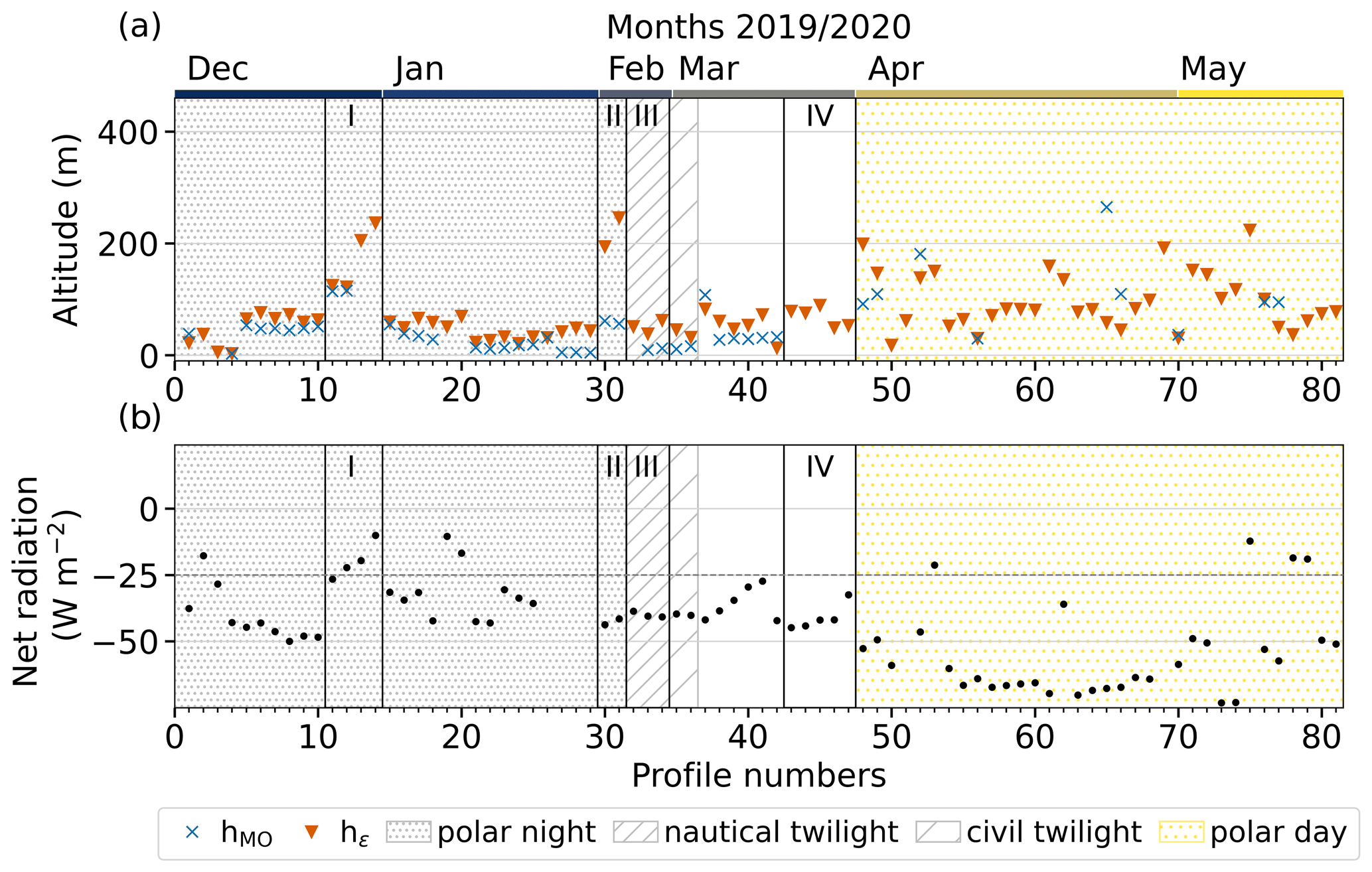
Figure 11 SML heights (a) estimated based on the MO method (h_MO) and direct in situ turbulence profiles (h_ε) as a function of profile number and (b) the net radiation F_net as observed at the surface. In addition to the profile numbers, the respective month of the year is indicated on the top axis in (a). Further, shading refers to daylight conditions similar to Fig. 1. Periods discussed in the text are marked as bounded and enumerated with roman numerals.

Figure 11 shows h_MO including h_ε as a reference (Fig. 11a) and the net radiation F_net (Fig. 11b) with a threshold of −25 W m⁻² separating cloudless from cloudy conditions. This plot shows qualitative agreement between h_MO and h_ε for cases with two or more subsequent values with F_net < −25 W m⁻² covering longer-lasting cloudless cases. That is particularly true for the polar night and twilight periods. However, h_MO is often slightly lower than h_ε. To determine the scaling height, we averaged over 30 min, thus comparing 30 min statistics with a “snapshot” of the atmosphere. We have tested shorter averaging periods (5 min) for profiles 6, 15, and 48. However, this does not explain all discrepancies between the two heights, so we assume that the variations between h_MO and h_ε are more likely to indicate atmospheric conditions. Nevertheless, h_MO represents the SML height well during wintertime and cloudless conditions.

In contrast, for profiles 11 to 14 on 29 December 2019 (period I in Fig. 11, see Fig. 3), we find F_net > −25 W m⁻², describing a more cloudy situation with increasing F_net. At the beginning of this cloudy period, we observe reasonable agreement between h_MO and h_ε, but eventually, with further increasing F_net, L becomes negative, and MO theory fails to predict an SML height. Therefore, with rapidly changing cloud cover, SML height determinations using MO theory are only partially successful. F_net observations can at least indicate these possible problems if no vertical profiles of thermodynamic or turbulent parameters are available.

During a short period on 6 February 2020 (profiles 30 and 31, period II), a situation with apparent disagreement between h_MO and h_ε, but F_net < −25 W m⁻² and L being positive, has been identified. This cloudless period was influenced by a LLJ, which added another source of turbulent kinetic energy well above the surface. The resulting profile of ε therefore never falls below the threshold for h_ε between the core of the LLJ and the surface, indicating a much higher SML height than h_MO.

With the beginning of twilight (15 February 2020, profiles 34 to 36, period III), the cloudless ABL was characterized by a surface inversion and an elevated inversion above, separated by a weakly stable to neutral stratified layer in between, as frequently observed in high latitudes during winter (Mauritsen, 2007). Below the elevated inversion, ε was always slightly above the threshold for h_ε, suggesting at least some vertical turbulent mixing. However, h_MO significantly underestimates the SML height under those conditions.

In the context of clouds, another particular situation may cause misinterpretation. Shallow ground fog within a neutrally stratified SML up to about 45 m capped by an inversion was observed in late March (profiles 46 to 51, period IV). The fog was optically quite thin, associated with F_net < −25 W m⁻². Due to the elevated inversion, the turbulence threshold was exceeded below 100 m. MO theory failed to predict an SML height because L<0.

The situation becomes even more complicated in the transition to polar day when the thermal stratification changes from rather stable to neutral or unstable, and the cloud situation – even with some foggy days – often becomes very complex. These conditions pose challenges for the MO method, especially at the end of the observation period when L is often negative, and thus no SML height can be determined.

4 Summary and conclusion

The main focus of this study is the evaluation of different methods for determining the surface mixing layer (SML) height for typical conditions observed in the central Arctic during MOSAiC in winter and early spring. The two typical observed conditions – cloudless with a near-surface temperature inversion and cloudy with an elevated inversion at the cloud top – were analyzed in detail. Further, the applicability of the different SML height determinations was investigated for both conditions individually since they offer partly fundamentally different preconditions.

A major advantage of our dataset is the high-resolution turbulence measurements, which allow direct estimations of the SML height under the basic assumption that the turbulent mixing originating from the surface ends at the height where the turbulence falls below a certain threshold, and the flow thus becomes quasi-laminar. Since this transition from a turbulent to an almost laminar layer occurs quite suddenly, this method is relatively robust concerning the choice of the threshold. This method is not based on any further assumptions and is thus used here as a reference method.

This reference height was used to apply the surface bulk Richardson number method and to derive the critical value Ri_bc for the conditions observed during the winter and spring of MOSAiC. It was found that an average value of Ri_bc=0.12 can be recommended. We also derived Ri_bc individually for the two ABL conditions (cloudless and cloudy). The differences between these values are minimal (about 7 % deviation) and therefore negligible. That we did not observe a difference in the Ri_bc for the two cases may be somewhat surprising at first glance since the sources of turbulence are different. For the cloudless case, we have mainly the shear-induced turbulence at the surface, whereas for the cloudy conditions, turbulence from the cloud top is added, and the two overlap. In addition, surface cooling, and hence stability, is reduced in the presence of clouds, leading to less suppressed wind-shear-driven turbulence. It should be taken into account that we have only determined one term of the energy balance equation with the measured energy dissipation, and therefore we cannot make any further statements about the spatial distribution of the turbulent kinetic energy, its sources, or vertical transport. This analysis would require much more complex measurements, including the precise three-dimensional wind vector for covariance measurements, which was not the intention of this work. As long as the conditions as described by the (bulk) Richardson number are sufficient for the existence (or generation or suppression) of turbulence (Ri_b<Ri_bc), the cause of turbulence generation is not of concern for the current study. Thus, the independence of the observed Ri_bc from turbulence generation in both cases (cloudy and cloudless ABL) is physically reasonable.

One of the main advantages of this work is that the Ri_b method can be applied directly to the regularly performed radiosonde ascents with the determined value Ri_bc=0.12. This approach provides reliable estimates of the SML height that are about 40 % lower compared to using the canonical value of Ri_bc=0.25 ($〈h_{R{i}_{\text{bc}}=\mathrm{0.25}}/h_{R{i}_{\text{bc}}=\mathrm{0.12}}〉$ = 1.407). This advantage is particularly important when turbulence measurements from the balloon are not available due to weather or other factors. However, the Ri_b method requires skin temperature measurements or reliable temperature measurements at a height of 2 m.

There are, of course, other limitations to this study that need to be considered when interpreting the results. For example, we were not able to quantify coupled versus decoupled clouds, which are often observed during the Arctic summer and could change the results. This raises the question of whether the often weak inversion, decoupling the sub-cloud layer from the surface layer, is sufficient to push the turbulence below the threshold value and thus to define the SML height and the height at which Ri_bc is determined. The answer to this question urgently requires comparable measurements in the Arctic summer, where these cases are more frequently observed. A valuable supplement to understanding the influence of coupling and decoupling is in situ cloud observations on the balloon.

Since the balloon-borne turbulence profiles are not continuously available, this does not allow for an adequate investigation of the evolution of the SML height. For this reason, we investigated the applicability of the Monin–Obukhov (MO) scaling theory to estimate the SML height. Applying MO to near-surface turbulent flux measurements from tower-based observations, SML heights can be estimated under certain assumptions and compared with the reference heights. Especially for the wintertime, when stable and cloudless conditions prevail, the MO method nicely complements the ABL characterization and provides reliable SML heights. Since the MO method is not applicable for additional sources of turbulence above the surface, such as cloud-top cooling or wind shear caused by LLJs, these limitations must be excluded by appropriate observations. Here, at least additional radiosondes are essential for an assessment, while determining surface fluxes alone would often lead to erroneous estimates of the SML height for our observations.

Another point to be considered is the sensitivity of Ri_bc to the selection of the lowest observation level. While the mean Ri_bc is 0.12 in this study for a 2 m temperature as the surface reference level, Ri_bc increases to 0.16 when the skin temperature is used as the surface-level temperature. Therefore, values taken from the literature should always be interpreted with the specifics of the applied approach taken into account.

Since Ri_bc does not seem to be universal for all field experiments and we do not yet know the exact cause of the sometimes considerable variability described in the literature, it will probably be necessary in the future to either determine Ri_bc individually for each experiment or to measure the SML height directly using turbulence measurements.

Unfortunately, our observations cannot answer other important questions, such as the temporal evolution of the SML height during the transition from cloudless to cloudy conditions and vice versa, because we do not have continuous observations during such an ABL evolution. A height estimation using the MO method is no longer applicable here due to the influence of the cloud. Furthermore, the time gap between consecutive balloon profiles was too large to observe this transition in detail. The latter holds for the tethered balloon turbulence profiles and even more for the radiosonde observations. Ultimately, we believe that only continuous turbulence profile measurements with an optimized measurement strategy can help answer such questions.

Finally, we come to the conclusion that turbulence profile measurements are the most reliable method to determine the SML height, but profile measurements with radiosondes can also be useful to either determine the SML height using the Richardson approach or to check the boundary conditions in combination with MO theory.

Appendix A

Table A1 Overview of tethered balloon-borne profiles. The profile number, start time, and derived SML heights are given using the direct in situ method (h_ε), the bulk Richardson number approach with the surface temperature at 2 m height and a critical value of Ri_bc = 0.12 ($h_{R{i}_{\mathrm{b}}}$), and the MO method (h_MO).