the Creative Commons Attribution 4.0 License.
the Creative Commons Attribution 4.0 License.
 | 26 Jan 2023
Using Orbiting Carbon Observatory-2 (OCO-2) column CO2 retrievals to rapidly detect and estimate biospheric surface carbon flux anomalies
Zhen Zhang
Yasuko Yoshida
Abhishek Chatterjee
Benjamin Poulter
The global carbon cycle is experiencing continued perturbations via increases in atmospheric carbon concentrations, which are partly reduced by terrestrial biosphere and ocean carbon uptake. Greenhouse gas satellites have been shown to be useful in retrieving atmospheric carbon concentrations and observing surface and atmospheric CO2 seasonal-to-interannual variations. However, limited attention has been placed on using satellite column CO2 retrievals to evaluate surface CO2 fluxes from the terrestrial biosphere without advanced inversion models at low latency. Such applications could be useful to monitor, in near real time, biosphere carbon fluxes during climatic anomalies like drought, heatwaves, and floods, before more complex terrestrial biosphere model outputs and/or advanced inversion modelling estimates become available. Here, we explore the ability of Orbiting Carbon Observatory-2 (OCO-2) column-averaged dry air CO2 (XCO2) retrievals to directly detect and estimate terrestrial biosphere CO2 flux anomalies using a simple mass-balance approach. An initial global analysis of surface–atmospheric CO2 coupling and transport conditions reveals that the western US, among a handful of other regions, is a feasible candidate for using XCO2 for detecting terrestrial biosphere CO2 flux anomalies. Using the CarbonTracker model reanalysis as a test bed, we first demonstrate that a well-established mass-balance approach can estimate monthly surface CO2 flux anomalies from XCO2 enhancements in the western United States. The method is optimal when the study domain is spatially extensive enough to account for atmospheric mixing and has favorable advection conditions with contributions primarily from one background region. We find that errors in individual soundings reduce the ability of OCO-2 XCO2 to estimate more frequent, smaller surface CO2 flux anomalies. However, we find that OCO-2 XCO2 can often detect and estimate large surface flux anomalies that leave an imprint on the atmospheric CO2 concentration anomalies beyond the retrieval error/uncertainty associated with the observations. OCO-2 can thus be useful for low-latency monitoring of the monthly timing and magnitude of extreme regional terrestrial biosphere carbon anomalies.
- Article
(3341 KB) - Full-text XML
-
Supplement
(1691 KB) - BibTeX
- EndNote


With ongoing anthropogenic emissions, atmospheric carbon dioxide concentrations continue to rise and alter the global climate system (Friedlingstein et al., 2022). A large contribution to the variability and trends of these CO2 concentrations is the uptake of carbon by the terrestrial biosphere (Ahlström et al., 2015; Poulter et al., 2014). The terrestrial biosphere typically acts as a sink but can become a strong source, or CO2 efflux, under climatic anomalies (Biederman et al., 2017; Zscheischler et al., 2014). Monitoring such surface CO2 flux anomalies in space and time is therefore essential to understand the drivers of atmospheric carbon dioxide concentrations and predict future climatic conditions.
However, observing CO2 fluxes across the terrestrial biosphere is a challenge. Carbon measurement networks are available but are spatially biased toward midlatitude locations with little coverage in the tropics (Schimel et al., 2015b). Atmospheric transport model assimilation efforts and land surface models are often used to quantify and monitor global carbon sources and sinks (Ott et al., 2015; Peters et al., 2007). However, these datasets typically have a longer latency and complex sources of error due to modelling assumptions about uncertain surface CO2 flux drivers and meteorological conditions, among others.
Greenhouse gas satellites are now available that can retrieve atmospheric column carbon concentrations, or dry-air column carbon dioxide (XCO2), across the globe at low latency. These include satellite instruments such as SCanning Imaging Absorption spectroMeter for Atmospheric CartograpHY (SCIAMACHY), Greenhouse Gases Observing Satellite (GOSAT), and the Orbiting Carbon Observatory-2 and -3 missions (OCO-2, OCO-3) (Bovensmann et al., 1999; Eldering et al., 2017b; Kuze et al., 2014; Reuter et al., 2011). Since these column retrievals are partly a function of surface CO2 fluxes (Keppel-Aleks et al., 2012; Parazoo et al., 2016) despite background variability driven partly by atmospheric transport (Basu et al., 2018; Hakkarainen et al., 2016; Schuh et al., 2019), previous studies have assimilated these XCO2 retrievals into atmospheric inversion model frameworks to improve surface CO2 flux estimates (Basu et al., 2013; Chevallier et al., 2014; Fraser et al., 2014; Halder et al., 2021; Houweling et al., 2015; Liu et al., 2017; Ott et al., 2015; Zabel et al., 2014). While a primary goal of the community has been to enable rapid detection, monitoring, and/or estimation of surface CO2 fluxes using the satellite XCO2 record, it has proved challenging due to the diversity of carbon sources and sinks as well as the effects of atmospheric mixing.
It has not been widely investigated whether satellites like OCO-2 can directly monitor the timing and magnitude of shorter monthly timescale climate–carbon feedback events, such as those that evolve in the terrestrial biosphere and generate regional and short-lived XCO2 enhancements. OCO-2 was designed to observe regional-scale carbon sources and sinks to provide a constraint on carbon cycle seasonal and interannual variability (Chen et al., 2021; Crisp et al., 2004; Eldering et al., 2017b; Lindqvist et al., 2015). For example, these satellite XCO2 retrievals have been used to evaluate effects of an event averaged over seasons or multiple years, such as El Niño–Southern Oscillation events and related biomass burning (Byrne et al., 2021; Chatterjee et al., 2017; Eldering et al., 2017b; Hakkarainen et al., 2019; Heymann et al., 2016; Liu et al., 2018; Patra et al., 2017). However, despite concern that the noise level of individual soundings would prevent direct monitoring of surface CO2 fluxes at finer scales (Chevallier et al., 2007; Eldering et al., 2017a; Miller et al., 2007), there is growing evidence that satellite XCO2 retrievals can directly detect and monitor surface CO2 fluxes, especially on smaller spatiotemporal scales. For example, satellite XCO2 can detect anthropogenic emission plumes from urban areas using spatially adjacent satellite soundings (Hakkarainen et al., 2016; Nassar et al., 2017; Reuter et al., 2019; Schwandner et al., 2017; Zheng et al., 2020). For natural emission sources, recent studies have interpreted monthly OCO-2 XCO2 anomalies without inversion models to understand the time evolution of climatic events (Chatterjee et al., 2017; Yin et al., 2020). As such, satellite XCO2 shows promise for directly monitoring the monthly timing and evolution of regional carbon–climate feedbacks from the biosphere at smaller spatiotemporal scales without model assimilation frameworks (Calle et al., 2019; He et al., 2018), especially if the signatures of these anomalies are large, localized over well-defined geographical regions, and detectable above the noise and uncertainty level of the observations.
Within the CO2 flux estimation literature, simple mass-balance approaches (also known as differential inversions) were widely used in the 1980s and 1990s (Conway et al., 1994; Enting and Mansbridge, 1989; Law, 1999; Siegenthaler and Joos, 1992; Siegenthaler and Oeschger, 1987). However, as the need grew for surface flux estimates discretized in space and time, the community moved from mass-balance techniques to more advanced synthesis inversions based on Green's functions, advanced atmospheric transport models, and state-space representations. Enting (2002) lays out other disadvantages of mass-balance techniques for estimating fine-scale fluxes, ranging from a failure of being able to resolve spatial detail to missing formalism for calculating uncertainty analysis, although the latter can be addressed via a bootstrapping approach (Conway et. al, 1994). Not surprisingly, recent efforts to estimate surface CO2 fluxes from OCO-2 XCO2 retrievals have involved transport models and inversions (Byrne et al., 2021; Liu et al., 2017; Palmer et al., 2019; Patra et al., 2017). The few studies estimating surface emissions directly from the XCO2 anomalies alone are empirical (rather than physically based mass-balance methods) in using statistical or machine learning relationships between XCO2 and surface CO2 fluxes (Heymann et al., 2016; Zhang et al., 2022) or are specific to point-source plumes at under kilometer scales rather than hundreds-of-kilometer-scale areal sources (Zheng et al., 2020). More recently, satellite methane concentration (XCH4) retrievals have been used to rapidly estimate surface methane fluxes using simple mass-balance approaches (Buchwitz et al., 2017b; Pandey et al., 2021). This makes sense given that CH4 fluxes are more spatially heterogeneous and have well-defined sources, unlike CO2 fluxes, which are more spatially homogeneous.
An equivalent approach using XCO2 in a mass balance may provide an ability to rapidly estimate regional total CO2 flux anomalies from the terrestrial biosphere. This ability to estimate a total CO2 flux anomaly would provide a rapid carbon cycle monitoring capability while waiting for more complex and complete biospheric model runs and atmospheric inversion estimates to become available (Ciais et al., 2014). Specifically, such a method could allow for near real-time monitoring of the duration, magnitude, and spatial extent of CO2 flux anomalies during extreme climatic events (Frank et al., 2015; Reichstein et al., 2013). Such applications are especially important for regional climate change hotspots like in southwestern North America where droughts and heatwaves are becoming more frequent and intense (Cook et al., 2015; Schwalm et al., 2012; Williams et al., 2022). This would also be beneficial for monitoring tropical biospheric fluxes (Byrne et al., 2017) which sequester the most global fossil fuel emissions but lack measurement networks (Liu et al., 2017; Schimel et al., 2015a). Analogously, a simple approach for estimating ecosystem water fluxes (i.e., triangle method; Carlson, 2007) has a legacy of continued use given its relatively sufficient accuracy for many applications compared to more complex land surface model approaches. Given the ongoing challenges of estimating terrestrial fluxes at large spatial scales, we anticipate that it will be similarly useful to develop simple total surface CO2 flux estimation approaches that are rapid, rely on observations alone (from remote sensing), do not require many modelling assumptions and ancillary data, and provide an independent estimate to evaluate model outputs when they eventually become available.
Here, we ask the following questions: can satellite-retrieved XCO2 be used with mass-balance approaches to directly detect and estimate terrestrial surface CO2 flux anomalies, especially from the biosphere? Can surface CO2 flux anomalies be monitored with XCO2 at sub-seasonal (i.e., monthly) scales? And which meteorological and spatial domain conditions are most favorable for estimating surface CO2 fluxes using such simple approaches? OCO-2 is chosen primarily due to its high precision and greater sensitivity to the lower atmosphere, which makes it more sensitive to surface CO2 fluxes and their anomalies than other greenhouse gas satellites (Eldering et al., 2017a). Recent algorithmic updates have also been shown to increase OCO-2 XCO2 retrievals' representation of biospheric CO2 fluxes at subcontinental scales (Miller and Michalak, 2020). Addressing these questions here can help assess whether greenhouse gas satellites like OCO-2 can be used to monitor biosphere carbon responses to climatic anomalies at sub-seasonal timescales and with low latency (within 1–2 months).
2.1 Datasets
The study includes three components to assess the potential for using XCO2 to directly evaluate monthly surface CO2 flux anomalies.
We first globally evaluated which regions provide favorable conditions to directly assess surface CO2 flux anomalies with observed XCO2 between September 2014 and December 2021 from the Orbiting Carbon Observatory-2 (OCO-2) aggregated to a 1∘ resolution (OCO-2). OCO-2 has an approximate 3 km2 resolution per sounding and 16 d revisit cycle with soundings at around 13:30 LT (local time). We use OCO-2 level 2, bias-corrected, retrospective reprocessing version 10 of XCO2 (OCO-2-Science-Team et al., 2020). Quality flags were used to remove soundings with poor retrievals. Along with OCO-2 XCO2, we also looked at MODIS-based FluxSat gross primary production (GPP) at a 1∘ × 1.25∘ resolution for the same time period (Joiner and Yoshida, 2020, 2021). We additionally evaluated monthly advection conditions using the Modern-Era Retrospective analysis for Research and Applications, version 2 (MERRA2) wind vectors at a 0.5∘ × 0.625∘ resolution (M2T3NVASM) (Gelaro et al., 2017; GMAO, 2015). Transport in the lower troposphere layer directly interacts with surface CO2 fluxes (Buchwitz et al., 2017b; Pandey et al., 2021). We thus compute lower troposphere advection by integrating wind velocities in a consistent number of atmosphere layers nearest to the surface, which at sea level results in integrating between the surface and about 700 mbar and at higher elevations integrating between the surface and about 600 mbar. Here, we assume that flux anomalies occurring near the surface have an immediate impact on CO2 concentrations near the surface, and if we examine the information content in the retrievals as the anomalies are occurring, we will be able to extract information about the flux anomalies before the signal gets diluted by atmospheric mixing. In this study, we refer to advection as the horizontal transport of air, especially that in the lower troposphere.
Second, we tested the ability of XCO2 to estimate surface CO2 flux anomalies using CarbonTracker model reanalysis (CT2019B) as a test bed, which assimilates tower eddy flux and satellite atmospheric observations into an atmospheric transport model and outputs hourly XCO2 and total surface CO2 fluxes from 2000 to 2018 (Peters et al., 2007). Tests performed using this model reanalysis dataset are meant to represent simulated “true” relationships between surface CO2 fluxes and XCO2 dynamics. However, we acknowledge model errors in this framework. A purely simulated environment with error-free conditions is not possible here because coupling between surface CO2 fluxes and XCO2 requires modelling and assumptions about atmospheric transport and emission physics. Therefore, we recognize that error in estimating surface CO2 flux anomalies from XCO2 will be partially a function of errors in modelling assumptions beyond that of errors incurred in the simple mass-balance approach.
Third, we assessed the ability of observed OCO-2 XCO2 to detect and estimate surface CO2 flux anomalies using the mass-balance technique. Observations of total surface CO2 fluxes are only sparsely located in space. We, therefore, independently estimated surface CO2 fluxes from a biosphere model, fire reanalysis, and anthropogenic emission repositories as a reference. The Lund-Potsdam-Jena (LPJ) dynamic global vegetation model was driven with MERRA2 reanalysis forcing to output CO2 flux from net biome production (NBP) between January 1980 and July 2021 (Gelaro et al., 2017; Sitch et al., 2003; Zhang et al., 2018). NBP models carbon fluxes from photosynthesis, respiration, land-use change, and fire. Since LPJ only evaluates fire dynamics at the annual scale and wildfire can rapidly evolve, fire carbon fluxes were obtained from Quick Fire Emissions Dataset (QFED) biomass burning emissions between 2000 and 2021 to account for monthly fire dynamics in the total carbon fluxes (Koster et al., 2015). Anthropogenic CO2 fluxes were obtained from CarbonMonitor for the western US region between 2019 and 2021 (Liu et al., 2020). Though only evaluating photosynthesis and no respiration or disturbance components, FluxSat GPP is also used here, because it provides another independent observation-based surface CO2 flux estimate to determine coupling between XCO2 anomalies and biospheric flux anomalies.
2.2 Region selection process
We first assessed the suitability of a given region for using XCO2 to detect and estimate surface CO2 flux anomalies using two different metrics. The first metric is the monthly Pearson's correlation coefficient between OCO-2 XCO2 and FluxSat GPP anomalies. The average climatology and long-term trend were subtracted from the raw time series to create an anomaly time series for both XCO2 and GPP. Statistically significant negative correlations show direct coupling between atmospheric CO2 and surface biospheric CO2 flux anomalies, suggesting favorable conditions to directly detect non-anthropogenic surface CO2 flux anomalies directly with independently observed XCO2. Though such satellite-based vegetation metrics are available at low latency, they are based on photosynthesis proxies. However, XCO2 can directly detect holistic terrestrial biosphere fluxes due to photosynthesis, respiration, and wildfires – we use this simple statistical correlation metric as an indicator of where across the globe XCO2 observations and biospheric fluxes have strong linkages.
The second metric evaluates the atmospheric transport conditions that not only allow for direct detection of surface CO2 flux anomalies with XCO2 but that also satisfy assumptions of a simple mass-balance approach for capturing surface CO2 flux anomaly from the XCO2 observations (see Sect. 2.4). This metric considers the temporal wind angle variability, the spatial wind angle variability, and whether there is an upwind water body source. Low spatial and temporal wind angle variability provide conditions that satisfy assumptions of the mass-balance method (see Sect. 2.4). Additionally, an upwind water body source typically has smaller, or less variable, surface CO2 flux anomalies with anomalies mainly due to transport and thus makes less surface-influenced background XCO2 conditions. The monthly MERRA2 wind vector angle in the lower troposphere is computed using the eastward direction as the zero-angle reference. The temporal wind angle variability is computed by taking the standard deviation of the monthly wind angle in each pixel. The spatial wind angle variability is computed by taking the standard deviation of the annual-averaged wind angle of the 20×20 pixel domain centered on each pixel (results are qualitatively similar varying the size of this domain). The temporal and spatial wind angle variability metrics are rescaled by dividing all pixels by the respective 95th percentile across the globe for each metric to transform values approximately to between zero and one. One minus both metrics is taken so that values nearer to one suggest more favorable, lower variability transport conditions. Finally, a water body source is determined by considering a 20×20 pixel domain around each target pixel, finding if water bodies exist in any of these pixels and determining if these water bodies are upwind of the central, target pixel. Pixels with an upwind water body are given a value of one or a value of zero if this condition is not met. To create a metric of “wind condition favorability”, these three metrics are objectively summed, creating a metric between approximately 0 and 3, with higher values indicating the best wind conditions for direct detection and estimation of surface CO2 flux anomalies with XCO2.
2.3 Wind vector analysis
Upon choosing the Western US region (33–49∘ N and 124–104∘ W) for the remainder of the analysis (see Sect. 3.1), we assessed the MERRA2 lower troposphere layer wind conditions to determine the direction, speed, and primary background region to consider for the mass-balance estimation approach. The spatially averaged wind direction and speed were determined within the region and at each of its four borders. The percentage of the background region's lower troposphere air entering the domain for each of its four borders was estimated as the ratio of the wind vector component entering the region to the total wind velocity.
2.4 XCO2-based surface CO2 flux anomaly estimation
First, XCO2 and CO2 surface fluxes in all cases were monthly averaged and spatially averaged, by averaging all pixels within the Western US target region (33–49∘ N and 124–104∘ W). For OCO-2, this included averaging all XCO2 soundings in this region over a month. Monthly XCO2 and surface CO2 fluxes were deseasonalized by averaging all months in the available time series into an average 12-month climatology. Given that XCO2 includes a strong annual increasing trend, each of the 12 months were individually, linearly detrended first before deseasonalizing as in Chatterjee et al. (2017).
Total surface CO2 flux anomalies were estimated from XCO2 anomalies in the Western US using a simple mass-balance approach previously applied to methane fluxes (Buchwitz et al., 2017b; Jacob et al., 2016; Varon et al., 2018):
Q is the surface CO2 flux anomalies in units of TgC month−1; ΔXCO2 (ppm) is the difference in XCO2 between the target domain and the background region (here, the Western US and Pacific Ocean, respectively). The full-column XCO2 is used here, which accounts for vertical transfer and atmospheric mixing of CO2 for the estimation approach. V is the ventilation wind velocity (in m s−1 units but converted to km month−1), which has been motivated previously to be best represented by lower-atmosphere horizontal winds (Buchwitz et al., 2017b; Pandey et al., 2021). Thus, while the full-column CO2 concentrations were evaluated, the wind speeds in the lower atmosphere are considered in the mass-balance model, given their greater degree of interaction with the CO2 fluxes at the surface. Here, V is the monthly averaged lower troposphere layer wind speed within the target region. L is the effective region length (km) meant to estimate the horizontal pathlength of the ventilation wind passing through the region and interacting with the surface flux. L was estimated as the square root of the target region area. The model parameter, C, represents assumptions that the CO2 fluxes are spatially homogeneous, and the ventilation wind is uniform across the region, which results in a linear increase of XCO2 spatially across the region. C is thus equal to 2 (unitless); Mexp (unitless) is the ratio of the target region's surface pressure to standard atmospheric pressure. MERRA2 and CarbonTracker surface pressure are used for the observational analysis and reanalysis test bed, respectively. M is TgC km−2 ppmXCO, which converts the atmospheric carbon dioxide mixing ratio (or its concentration) to a total column mass.
Previous demonstrations of Eq. (1) on methane fluxes evaluated the non-anomaly XCH4 enhancements (Buchwitz et al., 2017b; Pandey et al., 2021). In our main analysis, we have removed XCO2 seasonality here due to many sources of seasonal atmospheric CO2 variability (atmospheric and surface-based) that contribute to XCO2 that hinder causal attribution of XCO2 variability to surface anomalies. Monthly anomalies of XCO2 can thus be more directly attributed to surface CO2 flux anomalies than their raw variations can. However, we also evaluate non-anomaly XCO2 enhancements for comparison.
The ΔXCO2 estimated surface CO2 flux anomalies from Eq. (1) were compared with independently determined surface CO2 flux anomalies using the mean bias, root-mean-square difference (RMSD), and Pearson's correlation coefficient. Two comparisons were performed: one in a model reanalysis framework and another with OCO-2 observations. In the model reanalysis framework, the surface CO2 flux anomalies were estimated from CarbonTracker-output XCO2, wind velocity, and surface pressure using Eq. (1), and they were compared against CarbonTracker-output surface CO2 flux anomalies, which represent the total surface CO2 flux anomalies from both natural and anthropogenic sources. This reanalysis framework presents a test bed where the differences in XCO2 and surface CO2 flux outputs provide an estimate of the Eq. (1) model error, without being highly sensitive to other sources of error such as satellite XCO2 retrieval error as in the observational analysis. Using this framework, the target domain region size is varied to determine domain sizes that are more sensitive to errors. Additionally, horizontal wind speed and direction as well as vertical wind speed are related to Eq. (1) estimation errors, all of which are critical considerations of such pixel source mass-balance methods (Varon et al., 2018).
In the observational assessment, OCO-2 XCO2 is used to estimate surface CO2 flux anomalies along with MERRA2 lower troposphere wind velocity and surface pressure in Eq. (1). These XCO2-based surface CO2 flux anomaly estimates are compared to total surface CO2 flux anomalies, which were estimated using the sum of LPJ NBP model anomalies, QFED biomass burning anomalies, and CarbonMonitor fossil fuel estimates. As a postprocessing step of the LPJ model outputs that does not influence the LPJ simulation itself, LPJ NBP annual fire emissions were subtracted from the total LPJ NBP outputs, and monthly QFED biomass burning emissions were added, which results in NBP dynamics that include monthly instead of only annual fire emission dynamics. Though CarbonMonitor is only available over a short record, we used the record to determine that the proportion of anthropogenic flux anomalies in the Western US contribute less than 5 % to the surface anomalies (see Fig. S1 in the Supplement). Therefore, we define total flux anomaly estimates of CO2 in the observation-based assessment to be the sum of LPJ NBP and QFED biomass burning anomalies, acknowledging that there may be additional smaller deviations due to fossil fuel emissions.
2.5 XCO2-based surface CO2 flux anomaly detection
We estimated the XCO2 flux detection rate of surface efflux anomalies as the percentage of largest surface CO2 efflux anomalies (90th percentile) that XCO2 observes a positive anomaly. We evaluate this metric in all 1∘ pixels across the globe using OCO-2 XCO2 anomalies and FluxSat GPP to determine whether XCO2 anomalies can rapidly detect large surface biosphere CO2 flux anomalies from extreme events.
Generalizing the above approach, OCO-2-retrieved XCO2's ability to detect surface CO2 flux anomalies in the Western US is evaluated using the following:
The detection rate is the percentage of months that XCO2 anomaly enhancements (ΔXCO2) of a specified, y percentile, magnitude detects surface CO2 flux anomalies (Q) of a specified, x percentile, magnitude. N is a count of Western US domain-averaged pairs that satisfy the conditions in Eq. (2). Here, positive surface CO2 flux anomalies are toward the atmosphere. This metric provides a measure of information that a given XCO2 anomaly enhancement holds about a corresponding surface CO2 flux anomaly. This detection rate was compared to detection rates by chance, which are equal to 100−x. Equation (2) was used on both the observation-based and CarbonTracker test-bed data, with CarbonTracker tests serving as a “potential” or upper bound on performance given expected XCO2 observation error from OCO-2.
2.6 Estimation of retrieved XCO2 enhancement error
Given known limitations of potentially restrictive greenhouse gas satellite measurement and retrieval errors (Buchwitz et al., 2021), we estimated the XCO2 anomaly enhancement errors. OCO-2 XCO2 error standard deviation is approximately 0.6 ppm for a given observation and errors are assumed to be normally distributed (Eldering et al., 2017a). However, computing the ΔXCO2 (used in Eq. 1 estimation) and its error standard deviation involves consideration of monthly temporal averaging of XCO2, spatial averaging of XCO2 within the study domain, and subtracting two spatiotemporally averaged XCO2 anomalies from the target and background domains. We used a bootstrapping approach to randomly generate two vectors of XCO2 error values (including 20 observations within the Western US target region and 10 observations in the Pacific Ocean background region), which provides a spatially averaged XCO2 error for both the target and background regions. Both values are subtract to obtain an enhancement error.
3.1 Global region selection
Several regions show both observed coupling between XCO2 anomalies and biospheric surface CO2 flux anomalies (Fig. 1a) as well as favorable wind conditions for direct detection and estimation of surface CO2 flux anomalies with XCO2 (Figs. 1b and S2). These include, for example, southwestern North America (i.e., Western US), portions of north Africa, southern Africa, India, and portions of northern Australia.
The large observed coupling between XCO2 anomalies and biospheric surface CO2 flux anomalies in Fig. 1a in some regions suggests that terrestrial biospheric, non-anthropogenic carbon sources (i.e., photosynthesis, respiration, wildfire) influence XCO2 over expansive areas and that transport conditions do not obscure this connection between surface and atmospheric CO2. In these cases, OCO-2 XCO2 retrievals should be able to directly detect biospheric surface CO2 flux anomalies. These same regions commonly show tractable wind conditions (Fig. 1b): temporal and spatial wind direction variability is low, meaning that there is typically a single consistent background wind source rather than multiple background sources or a source that changes throughout the year. Furthermore, this background source may be located over water bodies, which tend to have less variable monthly CO2 surface fluxes compared to terrestrial sources. Therefore, wind condition favorability (Fig. 1b) partly supports why there is greater surface CO2 flux anomaly and XCO2 anomaly coupling (Fig. 1a). It also supports use of the mass-balance model (Eq. 1) which requires consistent boundary layer transport conditions for CO2 flux anomaly estimation. However, high wind condition favorability does not always result in coupling between XCO2 and biospheric surface CO2 flux anomalies. For example, western Europe has extensive anthropogenic CO2 fluxes, which results in weak coupling of XCO2 and biospheric surface CO2 flux anomalies despite tractable wind conditions. Ultimately, we speculate that favorable transport conditions (with less complex topography near the surface and consistent wind directions throughout the profile), high XCO2 retrieval quality, lower human footprint (i.e., from land-use change, fossil fuel emissions, etc.), and expanses of ecosystems with active photosynthesis (among others) all contribute to the higher metrics here. While it is unclear which factors contribute most, we anticipate that all of these conditions are needed in a region for our methods here to be feasibly applied.
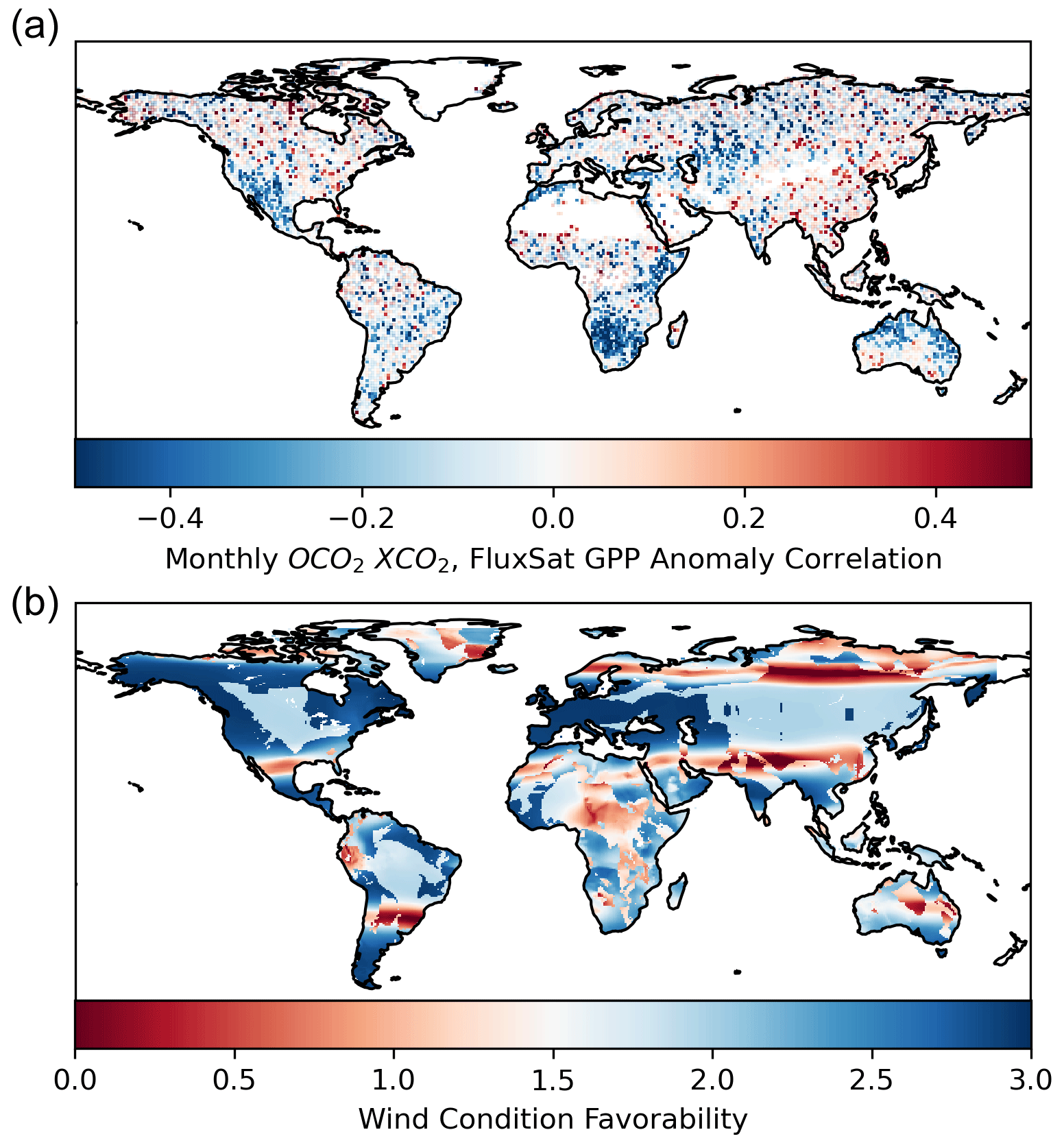
Figure 1(a) Observed coupling between terrestrial biosphere surface CO2 flux anomalies and atmospheric CO2 concentration anomalies. Monthly anomaly correlation between observed column CO2 (XCO2) from OCO-2 and observation-based FluxSat GPP (derived primarily from MODIS). Pixels that are not statistically significant (p < 0.05) are transparent. (b) Wind condition favorability index for application of simple mass-balance estimation approaches based on mean monthly lower troposphere (surface up to approximately 700 mbar) conditions from MERRA2. The index is high if the wind direction monthly temporal variability is low, wind direction spatial variability is low, and wind originates from water bodies. See Fig. S2 for mapped components contributing to the wind condition favorability metric.
For the remainder of the analysis, we primarily focus on the Western US, given its feasibility for use of XCO2 to detect and estimate biospheric surface CO2 flux anomalies. The Western US has an expanse of natural ecosystems that serve as a carbon sink (Biederman et al., 2017). It has also become a hotspot for droughts, including an ongoing decadal-scale megadrought (Cook et al., 2015; Schwalm et al., 2012; Williams et al., 2022). As such, any positive XCO2 anomalies are substantial, given that the mean OCO-2 XCO2 may be higher compared to pre-2000 when there was more nominal biospheric carbon uptake.
Given that we wish to use XCO2 anomalies in the Western US with only a simple source pixel mass-balance method and not an atmospheric transport model and/or assimilation framework to monitor surface CO2 flux anomalies, a detailed understanding of the existing advection conditions in the selected domain is highly critical, as emphasized by our analysis that follows. More detailed evaluation of the lower-atmosphere wind conditions in the Western US confirms tractable conditions as expected from Fig. 1 (see Fig. 2). Namely, monthly averaged winds consistently originate from a single background region in the Pacific Ocean and flow steadily and consistently (without greatly changing directions) west to east through the region (Figs. 2 and S3). Winds along its northern, southern, and eastern borders have little contribution to the Western US region. This suggests that Eq. (1) can be applied more confidently in assuming that only one background region contributes advection to the Western US. More detailed evaluation of the incoming advection from the Pacific Ocean reveals that incoming winds at the western border and throughout the region are consistently eastward and of non-negligible magnitude (Fig. S4). The exception is spring and summer months when winds in the Pacific Ocean partly shift to the south, and the speeds of eastward winds into and within the region are lower. By contrast, the advection conditions may be more complex in a region like the southeast US which experiences monthly changes in background source of incoming advection (Fig. S3). These variable background conditions and inconsistent wind directions may create large errors and lead to erroneous conclusions when applying Eq. (1).
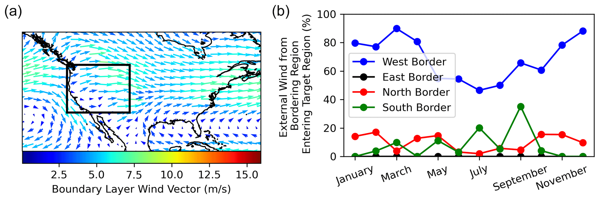
Figure 2(a) Annual mean lower troposphere (surface up to approximately 700 mbar) wind conditions from MERRA2. The Western US target domain is identified with borders. Averaged conditions in each month are shown in Fig. S3. (b) Proportion of wind vector entering region from each bordering region. Values do not add to 100 % as each border's wind vector is evaluated individually for its contribution to the Western US domain.
3.2 Reanalysis evaluation
Here, using CarbonTracker (CT2019B) model reanalysis as a test bed, we evaluate by how much the advection conditions present limitations for using Eq. (1) to estimate surface CO2 flux anomalies using XCO2 anomalies in the Western US. We tested the effect of domain area size, wind angle, and wind speed on the mass-balance surface CO2 flux anomaly estimation at monthly timescales.
Equation (1) was previously applied to smaller spatial scales (within a kilometer) to estimate emissions of spatially heterogeneous natural or urban methane plumes (Pandey et al., 2021). However, CO2 generally has more spatially homogeneous surface sources and sinks, and we wish to evaluate fluxes from terrestrial ecosystems that exceed tens of kilometers in spatial scales. We find that as our target regions become smaller, there is a decline in the ability to estimate surface CO2 flux anomalies with Eq. (1) (Fig. 3). This reduction in performance of the simple mass-balance model is expected as a smaller area will increase importance of turbulent mixing, especially from surface sources outside of the domain, compared to effects of mean horizontal ventilation wind, as was suggested previously (Varon et al., 2018). For example, with turbulent mixing on smaller spatial scales, large CO2 surface effluxes from surfaces adjacent to the region may mix with atmospheric CO2 within the region, causing a larger positive XCO2 anomaly than what can be expected from the surface contributions from within the small target domain itself. The decorrelation of the XCO2 surface flux anomaly estimates with the modelled surface CO2 flux anomalies with smaller surface areas supports this claim where external XCO2 anomaly variations may be contributing to the XCO2 anomalies within the domain (Fig. 3b). Ultimately, this target region size analysis motivates choosing larger target areas for application of Eq. (1) on CO2 flux anomaly estimation, especially over monthly timescales. Note that, in other parts of the globe, the area of surface–atmosphere CO2 coupling may be smaller (Fig. 1a). Figure 3 indicates that regions a quarter to half the size of that of our selected domain may still be feasible with only marginal increases in surface CO2 flux anomaly estimation errors.
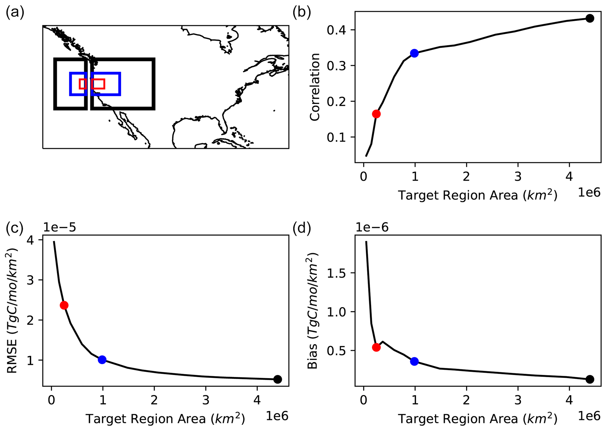
Figure 3Performance of the XCO2-based CO2 flux anomaly estimation when varying the target domain area. (a) Domain locations and sizes shown, where their domain border colors match the dot symbol colors in panels (b)–(d). (b) Correlation, (c) root mean square error, and (d) bias between the CO2 flux anomaly estimation with Eq. (1) based on XCO2 from CarbonTracker and the CarbonTracker monthly surface CO2 flux anomaly outputs, which is considered here as the reference.
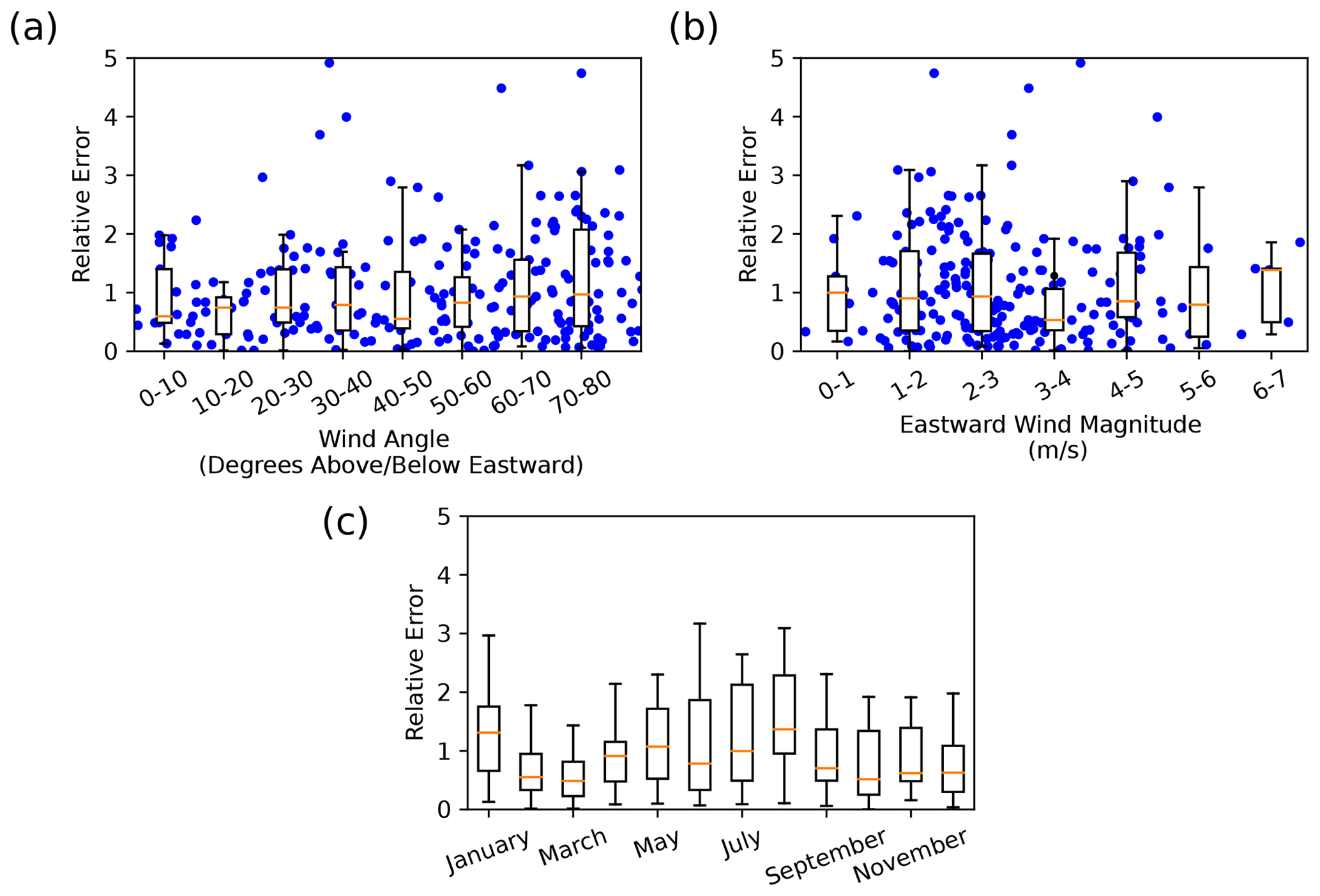
Figure 4Effect of monthly averaged horizontal ventilation wind conditions on CO2 flux anomaly estimation using CarbonTracker outputs. CO2 flux anomaly estimation error with respect to lower troposphere (a) wind angle and (b) wind speed. (c) CO2 flux anomaly estimation error averaged over each month of the year. Relative error is unitless and is the difference between each pair of CarbonTracker XCO2 flux anomaly estimates using Eq. (1) and reference CarbonTracker surface CO2 flux anomaly outputs, and it is divided by the standard deviation of the reference CarbonTracker surface CO2 flux anomaly outputs.
There is a general reduction in the mass-balance equation's (Eq. 1) ability to estimate surface CO2 flux anomalies with increasing wind angle (Fig. 4a). While absolute errors only weakly linearly increase with wind angle (r= 0.12; p value = 0.07) (RMSD's correlation with wind angle is r= 0.53, p value = 0.16 with eight bin samples), a more frequent occurrence of higher errors occurs above absolute angles of 60∘ from the eastward plane (Fig. 4a). As such, the partial shift to southward winds in the Pacific Ocean background during the summer months (Fig. S4b) may be the cause of seasonally increased surface CO2 flux anomaly estimation errors (Fig. 4c). This is expected because the advection of air from the Pacific Ocean into the Western US would be reduced, creating a disconnect between the atmospheric carbon concentrations of the Western US target region and Pacific Ocean in these months (Fig. 2). The effect of variations in monthly averaged wind speed appears to have less of an influence on errors than wind angle (Fig. 4b). Specifically, there is a correlation of 0.02 (p value = 0.7) between wind speed and absolute errors. Wind speed may become a larger error source when investigating shorter time steps or more spatially heterogeneous anthropogenic plumes (Jacob et al., 2016; Varon et al., 2018). Finally, the wind direction remains similar with height within the Western US and the CarbonTracker XCO2 enhancements occur mainly in the lower troposphere (Fig. S5). As such, this supports use of lower troposphere wind speeds for our analysis with the vertical profile of wind velocities not presenting a large source of error on CO2 flux detection and estimation in the case of the Western US.
The method appears robust to variations in vertical wind velocity, in part because XCO2 used here integrates the full atmospheric column and any vertical gradients of XCO2 anomalies. However, strong vertical winds toward the surface could prevent mixing of the surface CO2 flux with atmospheric CO2 and thus XCO2 may become decoupled from the surface. However, our investigation of these effects shows that there are rarely strong vertical monthly winds toward the surface in the Western US and that months with mean downwelling winds do not necessarily result in higher surface CO2 flux anomaly estimation errors with Eq. 1 (Fig. S6). Vertical atmospheric mixing over monthly timescales likely reduces errors related to vertical wind velocity, and we anticipate vertical wind velocity confounding effects can become more pronounced at shorter timescales.
Overall, the mass-balance estimation of surface CO2 flux anomalies with XCO2 (Eq. 1) is possible in the Western US (Fig. 5). XCO2 anomaly enhancements are positively correlated with surface CO2 flux anomalies (Fig. S7a), which extends to the positive correlation when estimating surface CO2 flux anomalies with Eq. (1) (Fig. 5). The comparison improves when consideration of winds that have a wind angle from the eastward reference of less than 60∘, which mainly removes summer months when Pacific Ocean winds shift toward the south (Fig. 5). However, an RMSD of ∼20 TgC month−1 suggests that the approach should be used mainly as a rapid, first estimation of surface CO2 flux anomalies.

Figure 5CarbonTracker XCO2 flux anomaly estimation overall performance in the Western US considering a spatially expansive target domain (latitude = 33–49∘ N, longitude = 124–104∘ W as shown in Fig. 2). Relationship between CarbonTracker surface CO2 flux anomaly outputs and mass-balance-based surface CO2 flux anomaly estimates based on CarbonTracker XCO2 anomaly enhancements. Only CarbonTracker data were used here where its XCO2, wind velocity, and pressure outputs were used to estimate surface CO2 flux anomalies with Eq. (1), which are compared to CarbonTracker total surface CO2 flux anomaly outputs. Legend shows correlations and root-mean-square differences between the CarbonTracker XCO2-based flux anomaly estimates (Eq. 1) and CarbonTracker surface CO2 flux anomaly outputs. “Eastward Wind Only” includes only data pairs when the incoming wind direction from the Pacific Ocean is between −60 and 60∘ angles from eastward reference direction.
We additionally show that the method can estimate surface CO2 fluxes using the non-anomaly XCO2 enhancements, especially when winds have a substantial eastward component (Fig. S7b). However, using the XCO2 anomalies removes seasonal XCO2 enhancement variability that may not be attributed to surface CO2 fluxes, which collapses the data pairs more along the 1:1 line (compare Figs. 5 and S7b).
Therefore, our tests with CarbonTracker model reanalysis reveal that XCO2 can indeed be used to viably estimate monthly surface CO2 flux anomalies with simple mass-balance approaches over spatial extents of natural ecosystems. However, the method requires favorable transport conditions. Namely, the region size must be large enough to account for atmospheric mixing that could dominate transport in smaller domains over monthly timescales. Additionally, based on Figs. 4 and 5 and assumptions of the mass-balance model, winds must flow consistently through the region with a similar direction. Given the need for XCO2 enhancements, the transport should originate from the same background source region within a given month rather than from multiple background regions. We speculate that the method may additionally work well in the Western US given the upwind ocean region (i.e., Pacific Ocean) tends to have relatively lower surface CO2 flux variability. Thus, the XCO2 enhancement variability will likely not be dominated by the background region's XCO2 variability. Finally, it is also critical that the OCO-2 retrieval availability in the target domain is representative enough to capture the flux anomalies occurring near the surface within a given month.
While the simple mass-balance approach appears suitable for use based on a model reanalysis framework, repeating the procedure with observations such as with OCO-2 presents additional challenges, such as due to observation error and spatiotemporal coverage or gaps. As such, CarbonTracker performance here effectively serves as an upper bound on predicting XCO2's ability to be coupled to surface CO2 flux anomalies, acknowledging modelling sources of error. We address these issues in the following section.
3.3 Observations evaluation
3.3.1 OCO-2 XCO2 coupling to surface CO2 flux anomalies
As expected from Fig. 1a, the spatially averaged XCO2 anomaly time series is negatively coupled to LPJ simulated net biome production and satellite-derived gross primary production anomalies (Fig. 6a). Observed XCO2 thus shows promise for directly detecting and estimating large-scale biospheric surface CO2 flux anomalies at low latency without the use of land surface and atmospheric transport assimilation models. Furthermore, the XCO2 coupling tends to increase when Pacific Ocean background XCO2 is subtracted from Western US XCO2 to account for transport conditions (Fig. 6a) (i.e., when XCO2 anomaly enhancements are used). This removes cases when the Western US XCO2 anomalies covary with Pacific Ocean background XCO2 anomalies like in 2015 to 2016, suggesting that Western US XCO2 variations were dominated by atmospheric transport rather than surface CO2 flux anomalies in this period (Fig. 6c). XCO2 anomaly enhancements remove these confounding effects (Fig. 6d). The coupling further increases when only months with mainly eastward flowing winds into the region are considered, at least for the total CO2 flux anomaly estimates (Fig. 6a) as expected from CarbonTracker model reanalysis tests (Fig. 5). This is because some large anomaly enhancements may occur in months that advection was not consistently flowing through the region (examples can be seen in late 2017 in Fig. 6c and d), thus requiring conditioning on wind angles.

Figure 6(a) Pearson correlation coefficients between the XCO2 anomalies and model-based total surface CO2 flux anomalies (LPJ model and QFED biomass burning) as well as with observation-based FluxSat ( p value < 0.05; * p value < 0.1). (b) Map of Western US and background Pacific Ocean background domain definitions. (c) Spatially averaged OCO-2 XCO2 anomalies in the Western US and background Pacific Ocean. (d) Western US XCO2 anomaly enhancements from the background Pacific Ocean OCO-2 XCO2 anomalies. Red symbols are months when the incoming wind direction from the Pacific Ocean was between −60 and 60∘ angles from eastward reference direction.
Even after isolating the effects of background Pacific Ocean XCO2 and abnormal advection conditions, the magnitude of these observation-based correlations of 0.32 (Fig. 6a) are lower than that of CarbonTracker reanalysis tests at a correlation of 0.54 (Fig. S7a). Indeed, the total CO2 flux anomalies are estimated by LPJ NBP and QFED burning biomass which include model estimations and assumptions with their own sets of errors. However, the surface–atmosphere carbon coupling is similar considering only photosynthesis fluxes from independently estimated GPP (Fig. 6a), which suggests a large role of the biosphere on the CO2 fluxes and that LPJ model error may not be the main contribution to the correlation reduction. We ultimately expect that a main source of reduction in coupling originates from OCO-2 retrieval error as well as gaps in the data, both spatially (due to cloud cover, aerosols, etc.) and temporally (due to the 16 d revisit frequency).
3.3.2 OCO-2 XCO2 estimation of monthly surface CO2 flux anomalies
Surface CO2 flux anomaly estimates from OCO-2 XCO2 using Eq. (1) weakly covary with modelled and observation-based surface CO2 flux anomalies (Fig. 7). In general, the simple mass-balance method increases its ability to estimate surface CO2 flux anomalies when conditioning on the “best” atmospheric transport conditions as shown across correlation, mean bias, and RMSD statistics (Fig. 7). However, the performance of the flux estimation method is reduced overall when using OCO-2 observations compared to CarbonTracker model reanalysis tests (shown for comparison in Fig. 7). This is expected for reasons mentioned above, and here we specifically investigate the role of OCO-2 XCO2 retrieval error on this reduction in performance.
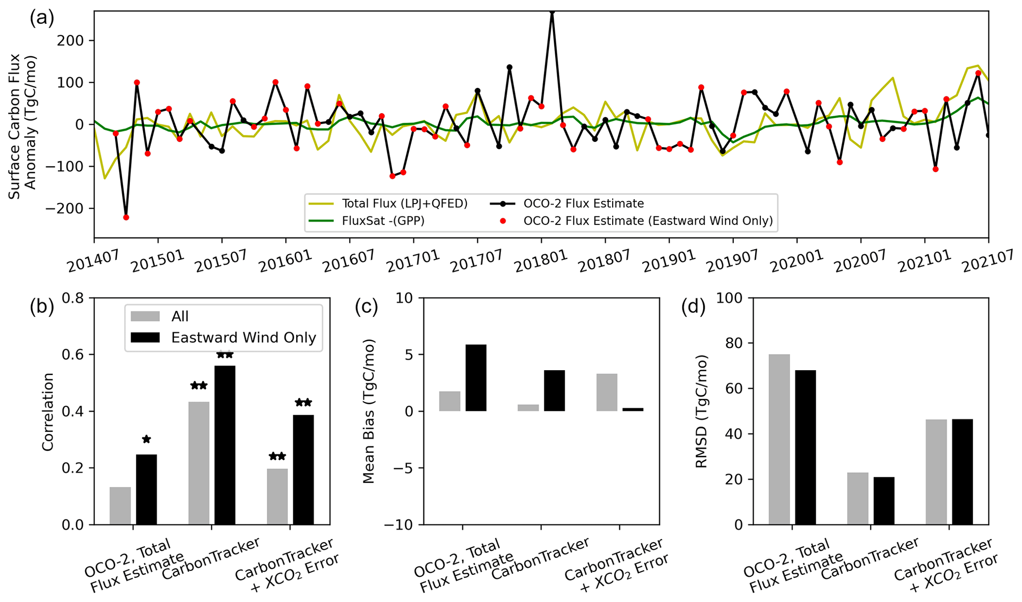
Figure 7(a) Spatially averaged OCO-2 XCO2 flux anomaly estimates compared to total CO2 flux estimate anomalies (LPJ model and QFED biomass burning) and FluxSat gross primary production anomalies. Positive anomalies of all metrics are fluxes away from the surface (note that GPP's sign was changed). Comparison statistics between OCO-2 flux anomaly estimates and LPJ NBP anomalies over 2014 to 2021 with (b) correlation ( p value < 0.05; * p value < 0.1), (c) mean bias, and (d) root mean square difference (RMSD). CarbonTracker comparisons are shown for reference as repeated from Fig. 5 but for 2000 to 2018. “CarbonTracker+XCO2 Error” includes simulated error added to CarbonTracker XCO2 anomaly outputs on the order of 0.2 ppm. The statistics are computed for all data pairs as well as only those considering “Eastward Wind Only” months when the incoming wind direction from the Pacific Ocean was between −60 and 60∘ angles from eastward reference direction.
We first estimate the error standard deviation of Western US XCO2 anomaly enhancements to be around 0.2 ppm based on a bootstrapping approach. This is a reduction from the 0.6 ppm error standard deviation for a given OCO-2 XCO2 retrieval (due to instrument and algorithmic error). This reduction is mainly due to averaging of 20 to 30 XCO2 retrievals a month within the study region. Note that using smaller domains with fewer XCO2 retrievals to average can result in XCO2 enhancement errors greater than a single XCO2 retrieval error due to subtracting two noisy XCO2 retrievals (subtracting two noisy XCO2 retrievals results in error of 0.8 ppm). The existence and magnitude of spatial autocorrelation is unknown, but weak spatial autocorrelation of errors could result in a potentially higher error standard deviation depending on the degree of spatial relation of errors; spatial autocorrelation of XCO2 errors removes some noise reduction benefits when averaging within a region but partially cancels errors because of spatial relation of errors of background and target regions. Ultimately, our conclusions remain the same over a range of XCO2 enhancement error estimates.
We show that reduced simple mass-balance flux anomaly estimation performance can largely be attributed to OCO-2 XCO2 retrieval error. Specifically, adding an approximate random 0.2 ppm XCO2 enhancement error standard deviation to CarbonTracker XCO2 outputs before applying Eq. (1) results in comparison statistics that approach the estimates based on the real OCO-2 observations (Fig. 7b–d). Other error sources likely also explain the reduced comparison between OCO-2-based estimates and surface modelled estimates including limited and/or inconsistent XCO2 spatiotemporal coverage, MERRA2 wind vector error, reference surface CO2 flux error (from LPJ biosphere model and QFED fire estimate error), and Eq. (1) mass-balance model errors. However, our test reveals that greenhouse gas satellite retrieval error is a dominant component of the overall error in estimating surface CO2 flux anomalies, even with reduced errors with spatiotemporal averaging. Ultimately, the retrieval error in OCO-2 XCO2 hinders reliable estimation of nominal monthly surface CO2 flux anomalies using rapid mass-balance approaches, as expected based on previous studies (Chevallier et al., 2007).
3.3.3 OCO-2 XCO2 detection of extreme surface CO2 flux anomalies
Although OCO-2 measurement noise limits estimation of smaller monthly surface CO2 flux anomalies using XCO2, OCO-2 XCO2 retrievals show promise in directly detecting the largest surface CO2 flux anomalies. Despite OCO-2 noise levels (of 0.2 to 0.6 ppm depending on averaging of individual soundings), large XCO2 anomalies above the noise are likely indicative of a large surface CO2 flux anomaly.
In the context of terrestrial biosphere extremes (i.e., droughts and heatwaves), we evaluate whether extreme surface biospheric CO2 efflux anomalies create a positive XCO2 anomaly in each global pixel (Fig. 8a; see Sect. 2.5). As expected from the global monthly correlation between biospheric CO2 flux and XCO2 anomalies (Fig. 1a), the same locations with a strong surface–atmospheric CO2 link are also those with the greatest detection rate of large CO2 effluxes (> 90th percentile) with positive XCO2 anomalies. These XCO2 detection rates in these same regions exceed 50 %, meaning OCO-2 will detect the surface CO2 flux signal as a positive XCO2 anomaly under extreme biosphere conditions, beyond only by chance. In the Western US, with increased satellite instrument accuracy, the detection rate could increase to 80 %, which is a detection rate potential estimated from CarbonTracker (Fig. 8b). Additionally, other regions like Morocco, southern Africa, and northern portions of Australia have detection rates of 80 % and above (Fig. 8b).
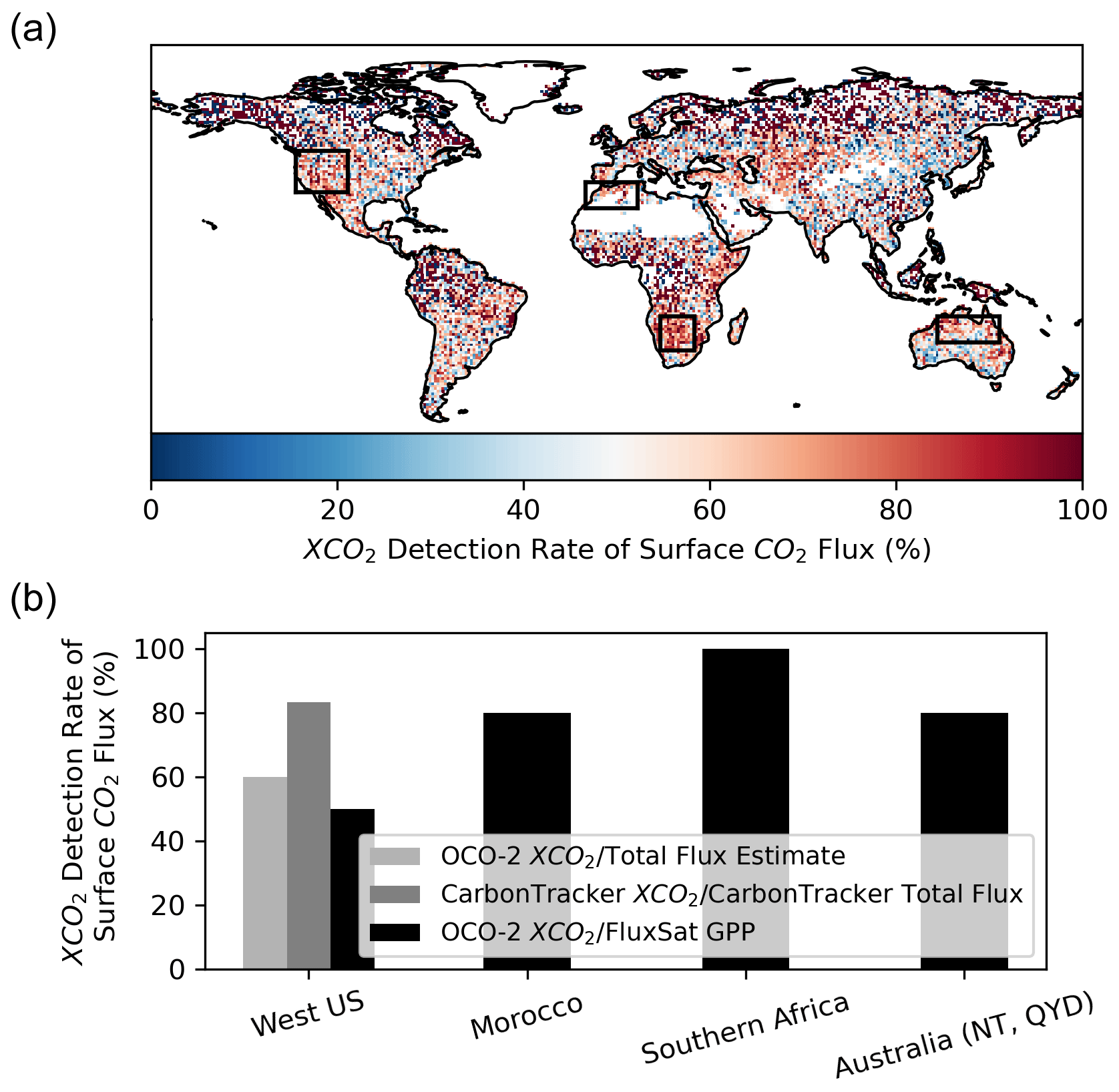
Figure 8OCO-2 XCO2 anomalies alone can detect extreme CO2 flux anomalies. OCO-2 detection rate of extreme surface CO2 flux anomalies (or positive XCO2 anomalies when surface CO2 efflux anomalies are the largest) (a) across the globe in each pixel and (b) within specific regions. The legend in (b) shows the datasets used to estimate the detection rate including pairs of OCO-2 XCO2 anomalies and total CO2 flux anomaly estimates from LPJ and QFED, pairs of CarbonTracker XCO2 anomalies and CarbonTracker total CO2 flux anomaly estimates, and pairs of OCO-2 XCO2 anomalies and photosynthesis flux anomaly estimates from FluxSat GPP.
A more detailed assessment reveals that OCO-2 XCO2 anomaly detection rates of surface CO2 flux anomalies are greater than by chance, especially for the most extreme surface CO2 flux anomalies (Fig. S8). As expected from correlations between surface CO2 flux anomalies and XCO2 anomaly enhancements, larger XCO2 anomaly enhancements are better able to detect surface CO2 flux anomalies than smaller XCO2 anomaly enhancements (Fig. S8a–S8c). CarbonTracker XCO2 anomaly enhancements can detect surface CO2 flux anomalies of at least the same percentile greater than by chance in nearly all cases without XCO2 observation-based noise (Fig. S8f). However, only the largest of OCO-2 XCO2 anomaly enhancements (> 90th percentile) can detect surface CO2 flux anomalies greater than by chance, demonstrating how OCO-2 retrieval error largely removes the surface CO2 flux information content of smaller magnitude XCO2 anomalies (Fig. S8d–S8e).
Ultimately, when a climatic event is ongoing and model outputs of surface CO2 fluxes are not yet available, OCO-2 XCO2 anomalies can be rapidly consulted. If a large XCO2 anomaly is detected, it can be used to motivate a more detailed investigation and/or monitoring campaign of the climatic event. This OCO-2 XCO2 anomaly detection potential has been recently realized (Hakkarainen et al., 2019) and at longer timescales where regional declines in fossil fuel emissions were detected with OCO-2 XCO2 anomalies on the order of 0.25–0.5 ppm during the COVID-19 pandemic (Weir et al., 2021), noting caveats of limited anomaly detection on the lower end of this range (Buchwitz et al., 2021; Chevallier et al., 2020). Most XCO2 anomalies attributed to the most extreme surface perturbations are below 1 ppm (Chatterjee et al., 2017; Crisp et al., 2017; Miller et al., 2007; Weir et al., 2021), which OCO-2 uncertainty may be able to detect as supported by our study (Eldering et al., 2017b; Wunch et al., 2017). However, other satellites like GOSAT and SCIAMACHY have estimated XCO2 retrieval uncertainty over 1 ppm (Buchwitz et al., 2017a; Butz et al., 2011), which may limit their ability to interpret even the strongest monthly XCO2 anomalies. As such, OCO-2 may provide an ability to monitor the monthly evolution of anomalous regional surface sources and sinks of CO2 more precisely than the earlier generation of spaceborne greenhouse gas instruments.
3.3.4 OCO-2 XCO2 estimation of extreme surface CO2 flux anomalies
We show that the mass-balance method (Eq. 1) approximately estimates the most extreme fluxes (> 90th percentile based on LPJ outputs) in the Western US (Fig. 9). The 2021 fluxes in March and June were part of an extreme Western US drought and heatwave event (Philip et al., 2021; Williams et al., 2022). The LPJ model and QFED wildfire estimates indicate that these total CO2 efflux anomalies increased to a peak in spring 2021 (Fig. 7a). In June 2021, the OCO-2-based CO2 flux anomaly estimate is 122 TgC month−1, while the independent total CO2 flux anomaly estimate from LPJ and QFED is 140 TgC month−1 (Fig. 9). Note that GPP anomalies are shown for comparison but are expected to be underestimates of the total effluxes in not including respiration and fire emissions. Therefore, the mass-balance method provides a viable method to rapidly estimate the extreme CO2 flux anomalies from a satellite observation source compared to more complex bottom-up biogeochemical modelling and advanced top-down inversion methods. In the months when XCO2-based CO2 flux anomalies did not compare with that estimated in 2020, especially in September 2020, the total CO2 flux anomaly estimate (from LPJ and QFED) potentially was positively biased when FluxSat GPP did not indicate a large biosphere CO2 flux anomaly (Figs. 7a and 9). Therefore, the extreme CO2 flux anomaly estimates from the biosphere model may have had model-related errors that resulted in the reduced comparison. However, OCO-2 flux estimation error is expected given the imperfect anomaly detection rates shown in Fig. 8. This is especially the case in May 2020 when both modelled NBP and satellite-based GPP indicated an efflux in May 2020 that OCO-2 did not detect.
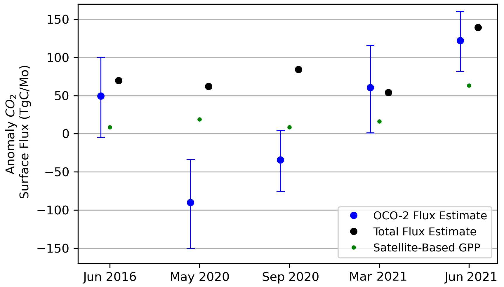
Figure 9OCO-2 can roughly estimate extreme surface CO2 flux anomalies. OCO-2 estimation of extreme surface CO2 flux anomalies in the Western US target domain. Total CO2 flux anomaly estimates are estimated from a combination of a dynamic global vegetation model (LPJ) and wildfire model reanalysis estimates. Error bars are determined from bootstrapped error estimates (see Sect. 3.3.2). Fossil fuel anomalies are negligible in magnitude compared to the biosphere and fire sources (see Fig. S1).
While a simple mass-balance approach does not supplant a rigorous flux estimate from inverse modelling and data assimilation methods, it serves as a rapid estimation approach that can be used within 1 to 2 months latency. This is a significant capability given that total surface CO2 flux anomaly estimates from biosphere model ensemble implementations or inverse modelling projects are often multi-month or multi-year efforts. As such, greenhouse gas satellites can be consulted for rapid monitoring and attribution to determine whether an ongoing extreme climatic anomaly (i.e., the Western US 2020–2021 drought) is creating substantial carbon cycle anomalies.
We demonstrate that OCO-2 satellite-retrieved XCO2 can be used with simple, yet effective, mass-balance frameworks to detect and estimate large biospheric CO2 flux anomalies at monthly timescales. The application tested here ultimately requires aggregating XCO2 over regional domains with careful consideration of transport conditions. Namely, the surface CO2 flux estimation mass-balance method using XCO2 improves when using larger spatial domains, when wind conditions are from the same background location, and wind flows consistently through the target domain. The larger spatial domain reduces errors due to turbulent atmospheric mixing of widespread surface CO2 sources that would otherwise hinder use of a source pixel mass-balance method at smaller spatial scales. Additionally, use of the larger area inherently requires aggregation of several XCO2 soundings which reduces the magnitude of XCO2 errors. While the Western US domain is evaluated here, our global regional assessment shows that these methods here are feasible for other locations with observed surface–atmosphere CO2 coupling and favorable wind conditions like portions of northern Africa, southern Africa, India, and northern Australia.
Satellite-observed XCO2 anomalies from OCO-2 are mainly useful for evaluating more extreme CO2 flux anomalies. While OCO-2 XCO2 retrieval error and observation gaps in space and time may hinder capturing smaller CO2 flux anomalies, we show that the timing and magnitude of extreme CO2 flux anomalies can be monitored with judicious use of the satellite data. In the absence of this error, the performance of these methods greatly improves as suggested by CarbonTracker reanalysis. Therefore, any improvement in XCO2 measurement and retrieval accuracy as well as improved coverage in space and time with upcoming greenhouse gas satellite missions (for example, GeoCarb) may extend the ability to globally monitor the timing and magnitude of biosphere anomalies at shorter timescales. Furthermore, even if advection conditions prevent use of the simple pixel source mass-balance method, extreme CO2 flux anomalies at least can be detected using only the observed monthly XCO2 anomaly within the target domain. In addition to the Western US study domain here, we show that this anomaly-only approach is feasible in other domains like southern Africa, Morocco, and northern Australia, thus enhancing the capability of the satellite data to contribute toward carbon monitoring systems.
The value of such a means to monitor and estimate total surface CO2 flux anomalies with satellite XCO2 is manifold. (1) It is simple in requiring few assumptions and ancillary datasets. (2) It is rapid and therefore can be used as a first estimate in extreme event monitoring efforts. (3) It uses XCO2 which integrates all surface CO2 flux sources, the components of which otherwise need to be estimated separately in bottom-up approaches. (4) Since it is based mainly on observations that are independent of land surface models, it can be used as an independent estimate to evaluate global model surface CO2 flux outputs. Nevertheless, the method comes with uncertainty due to instrument noise and atmospheric transport and should be used in tandem with other observed variables in low-latency analyses.
We recommend that future work further evaluate transport conditions and pixel source mass-balance flux estimation in other global regions we have identified here. Extensions of the method here should also be developed for regions with more complex transport conditions and anthropogenic influences (i.e., eastern US, western Europe). Ultimately, these methods should be developed for low-latency monitoring in known climate change hotspot regions, as is done here for the Western US hotspot, where more frequent and intense climate anomalies are expected in the future.
All datasets used here are freely available. CarbonTracker reanalysis data (CT2019B) are available at https://gml.noaa.gov/ccgg/carbontracker/CT2019B/ (Jacobson et al., 2020). MERRA2 reanalysis wind and pressure fields are available at https://doi.org/10.5067/SUOQESM06LPK (Global Modeling and Assimilation Office, 2015). The OCO-2 XCO2 retrievals and QFED outputs are available at https://doi.org/10.5067/E4E140XDMPO2 (OCO-2-Science-Team et al., 2020) and https://portal.nccs.nasa.gov/datashare/iesa/aerosol/emissions/QFED/v2.4r6/ (Koster et al., 2015), respectively. FluxSat GPP is available from https://doi.org/10.3334/ORNLDAAC/1835 (Joiner and Yoshida, 2021). The LPJ model code is publicly available at https://github.com/benpoulter/LPJ-wsl_v2.0 (last access: 15 September 2021; https://doi.org/10.5281/zenodo.4409331, Calle and Poulter, 2021).
The supplement related to this article is available online at: https://doi.org/10.5194/acp-23-1545-2023-supplement.
BP conceived the study. AFF conducted the analysis and wrote the article. BP and AC led the study. ZZ ran the LPJ model. YY provided GPP remote sensing retrievals and offered guidance on their interpretation. All authors contributed interpretations of figures and textual edits.
At least one of the (co-)authors is a member of the editorial board of Atmospheric Chemistry and Physics. The peer-review process was guided by an independent editor, and the authors also have no other competing interests to declare.
Publisher’s note: Copernicus Publications remains neutral with regard to jurisdictional claims in published maps and institutional affiliations.
The authors thank two anonymous reviewers for comments that improved the article. In addition, the authors also acknowledge the fruitful discussions and comments from the OCO-2 Flux MIP team on the feasibility and limitations of the simple mass-balance approach relative to the more advanced inverse modelling and data assimilation methods for estimating CO2 fluxes.
This research has been supported by the National Aeronautics and Space Administration (NASA Postdoctoral Program).
Andrew F. Feldman's research was supported by an appointment to the NASA Postdoctoral Program at the NASA Goddard Space Flight Center, administered by Oak Ridge Associated Universities under contract with NASA. Abhishek Chatterjee was also supported by NASA Carbon Monitoring System (grant no. 80NSSC20K0006).
This paper was edited by Christoph Gerbig and reviewed by two anonymous referees.
Ahlström, A., Raupach, M. R., Schurgers, G., Smith, B., Arneth, A., Jung, M., Reichstein, M., Canadell, J. G., Friedlingstein, P., Jain, A. K., Kato, E., Poulter, B., Sitch, S., Stocker, B. D., Viovy, N., Wang, Y. P., Wiltshire, A., Zaehle, S., and Zeng, N.: The dominant role of semi-arid ecosystems in the trend and variability of the land CO2 sink, Science, 348, 895–900, https://doi.org/10.1002/2015JA021022, 2015.
Basu, S., Guerlet, S., Butz, A., Houweling, S., Hasekamp, O., Aben, I., Krummel, P., Steele, P., Langenfelds, R., Torn, M., Biraud, S., Stephens, B., Andrews, A., and Worthy, D.: Global CO2 fluxes estimated from GOSAT retrievals of total column CO2, Atmos. Chem. Phys., 13, 8695–8717, https://doi.org/10.5194/acp-13-8695-2013, 2013.
Basu, S., Baker, D. F., Chevallier, F., Patra, P. K., Liu, J., and Miller, J. B.: The impact of transport model differences on CO2 surface flux estimates from OCO-2 retrievals of column average CO2, Atmos. Chem. Phys., 18, 7189–7215, https://doi.org/10.5194/acp-18-7189-2018, 2018.
Biederman, J. A., Scott, R. L., Bell, T. W., Bowling, D. R., Dore, S., Garatuza-Payan, J., Kolb, T. E., Krishnan, P., Krofcheck, D. J., Litvak, M. E., Maurer, G. E., Meyers, T. P., Oechel, W. C., Papuga, S. A., Ponce-Campos, G. E., Rodriguez, J. C., Smith, W. K., Vargas, R., Watts, C. J., Yepez, E. A., and Goulden, M. L.: CO2 exchange and evapotranspiration across dryland ecosystems of southwestern North America, Glob. Change Biol., 23, 4204–4221, https://doi.org/10.1111/gcb.13686, 2017.
Bovensmann, H., Burrows, J. P., Buchwitz, M., Frerick, J., Noël, S., Rozanov, V. V., Chance, K. V., and Goede, A. P. H.: SCIAMACHY: Mission objectives and measurement modes, J. Atmos. Sci., 56, 127–150, https://doi.org/10.1175/1520-0469(1999)056<0127:SMOAMM>2.0.CO;2, 1999.
Buchwitz, M., Reuter, M., Schneising, O., Hewson, W., Detmers, R. G., Boesch, H., Hasekamp, O. P., Aben, I., Bovensmann, H., Burrows, J. P., Butz, A., Chevallier, F., Dils, B., Frankenberg, C., Heymann, J., Lichtenberg, G., De Mazière, M., Notholt, J., Parker, R., Warneke, T., Zehner, C., Griffith, D. W. T., Deutscher, N. M., Kuze, A., Suto, H., and Wunch, D.: Global satellite observations of column-averaged carbon dioxide and methane: The GHG-CCI XCO2 and XCH4 CRDP3 data set, Remote Sens. Environ., 203, 276–295, https://doi.org/10.1016/j.rse.2016.12.027, 2017a.
Buchwitz, M., Schneising, O., Reuter, M., Heymann, J., Krautwurst, S., Bovensmann, H., Burrows, J. P., Boesch, H., Parker, R. J., Somkuti, P., Detmers, R. G., Hasekamp, O. P., Aben, I., Butz, A., Frankenberg, C., and Turner, A. J.: Satellite-derived methane hotspot emission estimates using a fast data-driven method, Atmos. Chem. Phys., 17, 5751–5774, https://doi.org/10.5194/acp-17-5751-2017, 2017b.
Buchwitz, M., Reuter, M., Noël, S., Bramstedt, K., Schneising, O., Hilker, M., Fuentes Andrade, B., Bovensmann, H., Burrows, J. P., Di Noia, A., Boesch, H., Wu, L., Landgraf, J., Aben, I., Retscher, C., O'Dell, C. W., and Crisp, D.: Can a regional-scale reduction of atmospheric CO2 during the COVID-19 pandemic be detected from space? A case study for East China using satellite XCO2 retrievals, Atmos. Meas. Tech., 14, 2141–2166, https://doi.org/10.5194/amt-14-2141-2021, 2021.
Butz, A., Guerlet, S., Hasekamp, O., Schepers, D., Galli, A., Aben, I., Frankenberg, C., Hartmann, J. -M., Tran, H., Kuze, A., Keppel-Aleks, G., Toon, G., Wunch, D., Wennberg, P., Deutscher, N., Griffith, D., Macatangay, R., Messe, J., and Warneke, T.: Toward accurate CO2 and CH4 observations from GOSAT, Geophys. Res. Lett., 38, L14812, https://doi.org/10.1029/2011GL047888, 2011.
Byrne, B., Jones, D. B. A., Strong, K., Zeng, Z. C., Deng, F., and Liu, J.: Sensitivity of CO2 surface flux constraints to observational coverage, J. Geophys. Res., 122, 6672–6694, https://doi.org/10.1002/2016JD026164, 2017.
Byrne, B., Liu, J., Lee, M., Yin, Y., Bowman, K. W., Miyazaki, K., Norton, A. J., Joiner, J., Pollard, D. F., Griffith, D. W. T., Velazco, V. A., Deutscher, N. M., Jones, N. B., and Paton-Walsh, C.: The carbon cycle of southeast Australia during 2019–2020: Drought, fires, and subsequent recovery, AGU Adv., 2, e2021AV000469, https://doi.org/10.1029/2021AV000469, 2021.
Calle, L. and Poulter, B.: Model code for the LPJ-wsl_v2.0 Dynamic Global Vegetation Model, Zenodo [code], https://doi.org/10.5281/zenodo.4409331, 2021.
Calle, L., Poulter, B., and Patra, P. K.: A segmentation algorithm for characterizing rise and fall segments in seasonal cycles: an application to XCO2 to estimate benchmarks and assess model bias, Atmos. Meas. Tech., 12, 2611–2629, https://doi.org/10.5194/amt-12-2611-2019, 2019.
Carlson, T.: An Overview of the “Triangle Method” for Estimating Surface Evapotranspiration and Soil Moisture from Satellite Imagery, Sensors, 7, 1612–1629, 2007.
Chatterjee, A., Gierach, M. M., Sutton, A. J., Feely, R. A., Crisp, D., Eldering, A., Gunson, M. R., O'Dell, C. W., Stephens, B. B., and Schimel, D. S.: Influence of El Niño on atmospheric CO2 over the tropical Pacific Ocean: Findings from NASA's OCO-2 mission, Science, 358, 6360, https://doi.org/10.1126/science.aam5776, 2017.
Chen, Z., Huntzinger, D. N., Liu, J., Piao, S., Wang, X., Sitch, S., Friedlingstein, P., Anthoni, P., Arneth, A., Bastrikov, V., Goll, D. S., Haverd, V., Jain, A. K., Joetzjer, E., Kato, E., Lienert, S., Lombardozzi, D. L., Mcguire, P. C., Melton, J. R., Nabel, J. E. M. S., Pongratz, J., Poulter, B., Tian, H., Wiltshire, A. J., Zaehle, S., and Miller, S. M.: Five years of variability in the global carbon cycle: comparing an estimate from the Orbiting Carbon Observatory-2 and process-based models, Environ. Res. Lett., 16, 054041, https://doi.org/10.1088/1748-9326/abfac1, 2021.
Chevallier, F., Bréon, F. M., and Rayner, P. J.: Contribution of the Orbiting Carbon Observatory to the estimation of CO2 sources and sinks: Theoretical study in a variational data assimilation framework, J. Geophys. Res.-Atmos., 112, D09307, https://doi.org/10.1029/2006JD007375, 2007.
Chevallier, F., Palmer, P. I., Feng, L., Boesch, H., O'Dell, C. W., and Bousquet, P.: Toward robust and consistent regional CO2 flux estimates from in situ and spaceborne measurements of atmospheric CO2, Geophys. Res. Lett., 41, 1065–1070, https://doi.org/10.1002/2013GL058772, 2014.
Chevallier, F., Zheng, B., Broquet, G., Ciais, P., Liu, Z., Davis, S. J., Deng, Z., Wang, Y., Bréon, F. M., and O'Dell, C. W.: Local Anomalies in the Column-Averaged Dry Air Mole Fractions of Carbon Dioxide Across the Globe During the First Months of the Coronavirus Recession, Geophys. Res. Lett., 47, e2020GL090244, https://doi.org/10.1029/2020GL090244, 2020.
Ciais, P., Dolman, A. J., Bombelli, A., Duren, R., Peregon, A., Rayner, P. J., Miller, C., Gobron, N., Kinderman, G., Marland, G., Gruber, N., Chevallier, F., Andres, R. J., Balsamo, G., Bopp, L., Bréon, F.-M., Broquet, G., Dargaville, R., Battin, T. J., Borges, A., Bovensmann, H., Buchwitz, M., Butler, J., Canadell, J. G., Cook, R. B., DeFries, R., Engelen, R., Gurney, K. R., Heinze, C., Heimann, M., Held, A., Henry, M., Law, B., Luyssaert, S., Miller, J., Moriyama, T., Moulin, C., Myneni, R. B., Nussli, C., Obersteiner, M., Ojima, D., Pan, Y., Paris, J.-D., Piao, S. L., Poulter, B., Plummer, S., Quegan, S., Raymond, P., Reichstein, M., Rivier, L., Sabine, C., Schimel, D., Tarasova, O., Valentini, R., Wang, R., van der Werf, G., Wickland, D., Williams, M., and Zehner, C.: Current systematic carbon-cycle observations and the need for implementing a policy-relevant carbon observing system, Biogeosciences, 11, 3547–3602, https://doi.org/10.5194/bg-11-3547-2014, 2014.
Conway, T. J., Tans, P. P., Waterman, L. S., Thoning, K. W., Kitzis, D. R., Maserie, K. A., and Zhang, N.: Evidence for interannual variability of the carbon cycle from the National Oceanic and Atmospheric Administration/Climate Monitoring and Diagnostics Laboratory Global Air Sampling Network, J. Geophys. Res., 99, 22831–22855, https://doi.org/10.1029/94jd01951, 1994.
Cook, B. I., Ault, T. R., and Smerdon, J. E.: Unprecedented 21st century drought risk in the American Southwest and Central Plains, Sci. Adv., 1, 1–7, https://doi.org/10.1126/sciadv.1400082, 2015.
Crisp, D., Atlas, R. M., Breon, F. M., Brown, L. R., Burrows, J. P., Ciais, P., Connor, B. J., Doney, S. C., Fung, I. Y., Jacob, D. J., Miller, C. E., O'Brien, D., Pawson, S., Randerson, J. T., Rayner, P., Salawitch, R. J., Sander, S. P., Sen, B., Stephens, G. L., Tans, P. P., Toon, G. C., Wennberg, P. O., Wofsy, S. C., Yung, Y. L., Kuang, Z., Chudasama, B., Sprague, G., Weiss, B., Pollock, R., Kenyon, D., and Schroll, S.: The Orbiting Carbon Observatory (OCO) mission, Adv. Sp. Res., 34, 700–709, https://doi.org/10.1016/j.asr.2003.08.062, 2004.
Crisp, D., Pollock, H. R., Rosenberg, R., Chapsky, L., Lee, R. A. M., Oyafuso, F. A., Frankenberg, C., O'Dell, C. W., Bruegge, C. J., Doran, G. B., Eldering, A., Fisher, B. M., Fu, D., Gunson, M. R., Mandrake, L., Osterman, G. B., Schwandner, F. M., Sun, K., Taylor, T. E., Wennberg, P. O., and Wunch, D.: The on-orbit performance of the Orbiting Carbon Observatory-2 (OCO-2) instrument and its radiometrically calibrated products, Atmos. Meas. Tech., 10, 59–81, https://doi.org/10.5194/amt-10-59-2017, 2017.
Eldering, A., O'Dell, C. W., Wennberg, P. O., Crisp, D., Gunson, M. R., Viatte, C., Avis, C., Braverman, A., Castano, R., Chang, A., Chapsky, L., Cheng, C., Connor, B., Dang, L., Doran, G., Fisher, B., Frankenberg, C., Fu, D., Granat, R., Hobbs, J., Lee, R. A. M., Mandrake, L., McDuffie, J., Miller, C. E., Myers, V., Natraj, V., O'Brien, D., Osterman, G. B., Oyafuso, F., Payne, V. H., Pollock, H. R., Polonsky, I., Roehl, C. M., Rosenberg, R., Schwandner, F., Smyth, M., Tang, V., Taylor, T. E., To, C., Wunch, D., and Yoshimizu, J.: The Orbiting Carbon Observatory-2: first 18 months of science data products, Atmos. Meas. Tech., 10, 549–563, https://doi.org/10.5194/amt-10-549-2017, 2017a.
Eldering, A., Wennberg, P. O., Crisp, D., Schimel, D. S., Gunson, M. R., Chatterjee, A., Liu, J., Schwandner, F. M., Sun, Y., O'Dell, C. W., Frankenberg, C., Taylor, T., Fisher, B., Osterman, G. B., Wunch, D., Hakkarainen, J., Tamminen, J., and Weir, B.: The Orbiting Carbon Observatory-2 early science investigations of regional carbon dioxide fluxes, Science, 358, 6360, https://doi.org/10.1126/science.aam5745, 2017b.
Enting, I. G.: Inverse Problems in Atmospheric Constituent Transport, Cambridge University Press, ISBN 9780511535741, 2002.
Enting, I. G. and Mansbridge, J. V.: Seasonal sources and sinks of atmospheric CO2. Direct inversion of filtered data, Tellus B, 41, 111–126, https://doi.org/10.3402/tellusb.v41i2.15056, 1989.
Frank, D., Reichstein, M., Bahn, M., Thonicke, K., Frank, D., Mahecha, M. D., Smith, P., van der Velde, M., Vicca, S., Babst, F., Beer, C., Buchmann, N., Canadell, J. G., Ciais, P., Cramer, W., Ibrom, A., Miglietta, F., Poulter, B., Rammig, A., Seneviratne, S. I., Walz, A., Wattenbach, M., Zavala, M. A., and Zscheischler, J.: Effects of climate extremes on the terrestrial carbon cycle: Concepts, processes and potential future impacts, Glob. Change Biol., 21, 2861–2880, https://doi.org/10.1111/gcb.12916, 2015.
Fraser, A., Palmer, P. I., Feng, L., Bösch, H., Parker, R., Dlugokencky, E. J., Krummel, P. B., and Langenfelds, R. L.: Estimating regional fluxes of CO2 and CH4 using space-borne observations of XCH4: XCO2, Atmos. Chem. Phys., 14, 12883–12895, https://doi.org/10.5194/acp-14-12883-2014, 2014.
Friedlingstein, P., Jones, M. W., O'Sullivan, M., Andrew, R. M., Bakker, D. C. E., Hauck, J., Le Quéré, C., Peters, G. P., Peters, W., Pongratz, J., Sitch, S., Canadell, J. G., Ciais, P., Jackson, R. B., Alin, S. R., Anthoni, P., Bates, N. R., Becker, M., Bellouin, N., Bopp, L., Chau, T. T. T., Chevallier, F., Chini, L. P., Cronin, M., Currie, K. I., Decharme, B., Djeutchouang, L. M., Dou, X., Evans, W., Feely, R. A., Feng, L., Gasser, T., Gilfillan, D., Gkritzalis, T., Grassi, G., Gregor, L., Gruber, N., Gürses, Ö., Harris, I., Houghton, R. A., Hurtt, G. C., Iida, Y., Ilyina, T., Luijkx, I. T., Jain, A., Jones, S. D., Kato, E., Kennedy, D., Klein Goldewijk, K., Knauer, J., Korsbakken, J. I., Körtzinger, A., Landschützer, P., Lauvset, S. K., Lefèvre, N., Lienert, S., Liu, J., Marland, G., McGuire, P. C., Melton, J. R., Munro, D. R., Nabel, J. E. M. S., Nakaoka, S.-I., Niwa, Y., Ono, T., Pierrot, D., Poulter, B., Rehder, G., Resplandy, L., Robertson, E., Rödenbeck, C., Rosan, T. M., Schwinger, J., Schwingshackl, C., Séférian, R., Sutton, A. J., Sweeney, C., Tanhua, T., Tans, P. P., Tian, H., Tilbrook, B., Tubiello, F., van der Werf, G. R., Vuichard, N., Wada, C., Wanninkhof, R., Watson, A. J., Willis, D., Wiltshire, A. J., Yuan, W., Yue, C., Yue, X., Zaehle, S., and Zeng, J.: Global Carbon Budget 2021, Earth Syst. Sci. Data, 14, 1917–2005, https://doi.org/10.5194/essd-14-1917-2022, 2022.
Gelaro, R., McCarty, W., Suárez, M. J., Todling, R., Molod, A., Takacs, L., Randles, C. A., Darmenov, A., Bosilovich, M. G., Reichle, R., Wargan, K., Coy, L., Cullather, R., Draper, C., Akella, S., Buchard, V., Conaty, A., da Silva, A. M., Gu, W., Kim, G. K., Koster, R., Lucchesi, R., Merkova, D., Nielsen, J. E., Partyka, G., Pawson, S., Putman, W., Rienecker, M., Schubert, S. D., Sienkiewicz, M., and Zhao, B.: The modern-era retrospective analysis for research and applications, version 2 (MERRA-2), J. Climate, 30, 5419–5454, https://doi.org/10.1175/JCLI-D-16-0758.1, 2017.
Global Modeling and Assimilation Office (GMAO): MERRA-2 tavg3_3d_asm_Nv: 3d, 3-Hourly, Time-Averaged, Model-Level, Assimilation, Assimilated Meteorological Fields V5.12.4, Greenbelt, MD, USA, Goddard Earth Sciences Data and Information Services Center (GES DISC) [data set], https://doi.org/10.5067/SUOQESM06LPK, 2015.
GMAO: MERRA-2 inst1_2d_asm_Nx: 2d,1-Hourly,Instantaneous,Single-Level,Assimilation,Single-Level Diagnostics V5.12.4, Greenbelt, MD, USA, Goddard Earth Sciences Data and Information Services Center (GES DISC) [data set], https://doi.org/10.5067/3Z173KIE2TPD, 2015.
Hakkarainen, J., Ialongo, I., and Tamminen, J.: Direct space-based observations of anthropogenic CO2 emission areas from OCO-2, Geophys. Res. Lett., 43, 11400–11406, https://doi.org/10.1002/2016GL070885, 2016.
Hakkarainen, J., Ialongo, I., Maksyutov, S., and Crisp, D.: Analysis of four years of global XCO2 anomalies as seen by Orbiting Carbon Observatory-2, Remote Sens., 11, 1–20, https://doi.org/10.3390/RS11070850, 2019.
Halder, S., Tiwari, Y. K., Valsala, V., Sijikumar, S., Janardanan, R., and Maksyutov, S.: Benefits of satellite XCO2 and newly proposed atmospheric CO2 observation network over India in constraining regional CO2 fluxes, Sci. Total Environ., 812, 151508, https://doi.org/10.1016/j.scitotenv.2021.151508, 2021.
He, Z., Lei, L., Welp, L. R., Zeng, Z. C., Bie, N., Yang, S., and Liu, L.: Detection of spatiotemporal extreme changes in atmospheric CO2 concentration based on satellite observations, Remote Sens., 10, 839, https://doi.org/10.3390/rs10060839, 2018.
Heymann, J., Reuter, M., Buchwitz, M., Schneising, O., Bovensmann, H., Burrows, J. P., Massart, S., Kaiser, J. W., and Crisp, D.: CO2 emission of Indonesian fires in 2015 estimated from satellite-derived atmospheric CO2 concentrations, Geophys. Res. Lett., 44, 1537–1544, https://doi.org/10.1002/2016GL072042, 2016.
Houweling, S., Baker, D., Basu, S., Boesch, H., Butz, A., Chevallier, F., Deng, F., Dlugokencky, E. J., Feng, L., Ganshin, A., Hasekamp, O., Jones, D., Maksyutov, S., Marshall, J., Oda, T., O'Dell, C. W., Oshchepkov, S., Palmer, P. I., Peylin, P., Poussi, Z., Reum, F., Takagi, H., Yoshida, Y., and Zhuravlev, R.: An intercomparison of inversemodels for estimating sources and sinks of CO2 using GOSAT measurements, J. Geophys. Res., 120, 5253–5266, https://doi.org/10.1002/2014JD022962, 2015.
Jacob, D. J., Turner, A. J., Maasakkers, J. D., Sheng, J., Sun, K., Liu, X., Chance, K., Aben, I., McKeever, J., and Frankenberg, C.: Satellite observations of atmospheric methane and their value for quantifying methane emissions, Atmos. Chem. Phys., 16, 14371–14396, https://doi.org/10.5194/acp-16-14371-2016, 2016.
Jacobson, A. R., Schuldt, K. N., Miller, J. B., Oda, T., Tans, P., Andrews, A., Mund, J., Ott, L., Collatz, G. J., Aalto, T., Afshar, S., Aikin, K., Aoki, S., Apadula, F., Baier, B., Bergamaschi, P., Beyersdorf, A., Biraud, S. C., Bollenbacher, A., Bowling, D., Brailsford, G., Abshire, J. B., Chen, G., Chen, H., Chmura, L., Sites Climadat., Colomb, A., Conil, S., Cox, A., Cristofanelli, P., Cuevas, E., Curcoll, R., Sloop, C. D., Davis, K., Wekker, S. D., Delmotte, M., DiGangi, J. P., Dlugokencky, E., Ehleringer, J., Elkins, J. W., Emmenegger, L., Fischer, M. L., Forster, G., Frumau, A., Galkowski, M., Gatti, L. V., Gloor, E., Griffis, T., Hammer, S., Haszpra, L., Hatakka, J., Heliasz, M., Hensen, A., Hermanssen, O., Hintsa, E., Holst, J., Jaffe, D., Karion, A., Kawa, S. R., Keeling, R., Keronen, P., Kolari, P., Kominkova, K., Kort, E., Krummel, P., Kubistin, D., Labuschagne, C., Langenfelds, R., Laurent, O., Laurila, T., Lauvaux, T., Law, B., Lee, J., Lehner, I., Leuenberger, M., Levin, I., Levula, J., Lin, J., Lindauer, M., Loh, Z., Lopez, M., Luijkx, I. T., Lund Myhre, C., Machida, T., Mammarella, I., Manca, G., Manning, A., Manning, A., Marek, M. V., Marklund, P., Martin, M. Y., Matsueda, H., McKain, K., Meijer, H., Meinhardt, F., Miles, N., Miller, C. E., Molder, M., Montzka, S., Moore, F., Morgui, J.-A., Morimoto, S., Munger, B., Necki, J., Newman, S., Nichol, S., Niwa, Y., ODoherty, S., Ottosson-Lofvenius, M., Paplawsky, B., Peischl, J., Peltola, O., Pichon, J.-M., Piper, S., Plass-Dolmer, C., Ramonet, M., Reyes-Sanchez, E., Richardson, S., Riris, H., Ryerson, T., Saito, K., Sargent, M., Sasakawa, M., Sawa, Y., Say, D., Scheeren, B., Schmidt, M., Schmidt, A., Schumacher, M., Shepson, P., Shook, M., Stanley, K., Steinbacher, M., Stephens, B., Sweeney, C., Thoning, K., Torn, M., Turnbull, J., Tørseth, K., Bulk, P. V. D., Dinther, D. V., Vermeulen, A., Viner, B., Vitkova, G., Walker, S., Weyrauch, D., Wofsy, S., Worthy, D., Young, D., and Zimnoch, M.: CarbonTracker CT2019B, NOAA Global Monitoring Laboratory [data set], https://gml.noaa.gov/ccgg/carbontracker/CT2019B/ (last access: 1 May 2022), 2020.
Joiner, J. and Yoshida, Y.: Satellite-based reflectances capture large fraction of variability in global gross primary production (GPP) at weekly time scales, Agr. Forest Meteorol., 291, 108092, https://doi.org/10.1016/j.agrformet.2020.108092, 2020.
Joiner, J. and Yoshida, Y.: Global MODIS and FLUXNET-derived Daily Gross Primary Production, V2, ORNL DAAC [data set], Oak Ridge, Tennessee, USA, https://doi.org/10.3334/ORNLDAAC/1835, 2021.
Joiner, J. and Yoshida, Y.: Global MODIS and FLUXNET-derived Daily Gross Primary Production, V2, ORNL DAAC [data set], Oak Ridge, Tennessee, USA, https://doi.org/10.3334/ORNLDAAC/1835, 2021.
Keppel-Aleks, G., Wennberg, P. O., Washenfelder, R. A., Wunch, D., Schneider, T., Toon, G. C., Andres, R. J., Blavier, J.-F., Connor, B., Davis, K. J., Desai, A. R., Messerschmidt, J., Notholt, J., Roehl, C. M., Sherlock, V., Stephens, B. B., Vay, S. A., and Wofsy, S. C.: The imprint of surface fluxes and transport on variations in total column carbon dioxide, Biogeosciences, 9, 875–891, https://doi.org/10.5194/bg-9-875-2012, 2012.
Koster, R. D., Darmenov, A., and Silva, A.: The Quick Fire Emissions Dataset (QFED): Documentation of Versions 2.1, 2.2 and 2.4. Volume 38; Technical Report Series on Global Modeling and Data Assimilation, https://ntrs.nasa.gov/citations/20180005253 (last access: 15 June 2022), 2015.
NEU Koster, R. D., Darmenov, A., and Silva, A.: The Quick Fire Emis- sions Dataset (QFED): Documentation of Versions 2.1, 2.2 and 2.4. Volume 38, Technical Report Series on Global Modeling and Data Assimilation, https://portal.nccs.nasa.gov/datashare/iesa/aerosol/emissions/QFED/v2.4r6/ (last access: 15 November 2021), 2015.
Kuze, A., Taylor, T. E., Kataoka, F., Bruegge, C. J., Crisp, D., Harada, M., Helmlinger, M., Inoue, M., Kawakami, S., Kikuchi, N., Mitomi, Y., Murooka, J., Naitoh, M., O'Brien, D. M., O'Dell, C. W., Ohyama, H., Pollock, H., Schwandner, F. M., Shiomi, K., Suto, H., Takeda, T., Tanaka, T., Urabe, T., Yokota, T., and Yoshida, Y.: Long-term vicarious calibration of GOSAT short-wave sensors: Techniques for error reduction and new estimates of radiometric degradation factors, IEEE T. Geosci. Remote, 52, 3991–4004, https://doi.org/10.1109/TGRS.2013.2278696, 2014.
Law, R. M.: CO2 sources from a mass-balance inversion: Sensitivity to the surface constraint, Tellus B, 51, 254–265, https://doi.org/10.3402/tellusb.v51i2.16281, 1999.
Lindqvist, H., O'Dell, C. W., Basu, S., Boesch, H., Chevallier, F., Deutscher, N., Feng, L., Fisher, B., Hase, F., Inoue, M., Kivi, R., Morino, I., Palmer, P. I., Parker, R., Schneider, M., Sussmann, R., and Yoshida, Y.: Does GOSAT capture the true seasonal cycle of carbon dioxide?, Atmos. Chem. Phys., 15, 13023–13040, https://doi.org/10.5194/acp-15-13023-2015, 2015.
Liu, J., Bowman, K. W., Schimel, D. S., Parazoo, N. C., Jiang, Z., Lee, M., Bloom, A. A., Wunch, D., Frankenberg, C., Sun, Y., O'Dell, C. W., Gurney, K. R., Menemenlis, D., Gierach, M., Crisp, D., and Eldering, A.: Contrasting carbon cycle responses of the tropical continents to the 2015–2016 El Niño, Science, 358, 6360, https://doi.org/10.1126/science.aam5690, 2017.
Liu, J., Bowman, K., Parazoo, N. C., Bloom, A. A., Wunch, D., Jiang, Z., Gurney, K. R., and Schimel, D.: Detecting drought impact on terrestrial biosphere carbon fluxes over contiguous US with satellite observations, Environ. Res. Lett., 13, 095003, https://doi.org/10.1088/1748-9326/aad5ef, 2018.
Liu, Z., Ciais, P., Deng, Z., Lei, R., Davis, S. J., Feng, S., and Zheng, B.: Near-real-time monitoring of global CO2 emissions reveals the effects of the COVID-19 pandemic, Nat. Commun., 11, 5172, https://doi.org/10.1038/s41467-020-18922-7, 2020.
Miller, C. E., Crisp, D., DeCola, P. L., Olsen, S. C., Randerson, J. T., Michalak, A. M., Alkhaled, A., Rayner, P., Jacob, D. J., Suntharalingam, P., Jones, D. B. A., Denning, A. S., Nicholls, M. E., Doney, S. C., Pawson, S., Boesch, H., Connor, B. J., Fung, I. Y., O'Brien, D., Salawitch, R. J., Sander, S. P., Sen, B., Tans, P., Toon, G. C., Wennberg, P. O., Wofsy, S. C., Yung, Y. L., and Law, R. M.: Precision requirements for space-based XCO2 data, J. Geophys. Res.-Atmos., 112, D10314, https://doi.org/10.1029/2006JD007659, 2007.
Miller, S. M. and Michalak, A. M.: The impact of improved satellite retrievals on estimates of biospheric carbon balance, Atmos. Chem. Phys., 20, 323–331, https://doi.org/10.5194/acp-20-323-2020, 2020.
Nassar, R., Hill, T. G., McLinden, C. A., Wunch, D., Jones, D. B. A., and Crisp, D.: Quantifying CO2 Emissions From Individual Power Plants From Space, Geophys. Res. Lett., 44, 10045–10053, 2017.
OCO-2-Science-Team, Gunson, M., and Eldering, A.: OCO-2 Level 2 bias-corrected XCO2 and other select fields from the full-physics retrieval aggregated as daily files, Retrospective processing V10r, Greenbelt, MD, USA, Goddard Earth Sciences Data and Information Services Center (GES DISC) [data set], https://doi.org/10.5067/E4E140XDMPO2, 2020.
Ott, L. E., Pawson, S., Collatz, G. J., Gregg, W. W., Menemenlis, D., Brix, H., Rousseaux, C. S., Bowman, K. W., Liu, J., Eldering, A., Gunson, M. R., and Kawa, S. R.: Assessing the magnitude of CO2 flux uncertainty in atmospheric CO2 records using products from NASA's Carbon Monitoring Flux Pilot Project, J. Geophys. Res.-Atmos., 120, 734–765, https://doi.org/10.1038/175238c0, 2015.
Palmer, P. I., Feng, L., Baker, D., Chevallier, F., Bösch, H., and Somkuti, P.: Net carbon emissions from African biosphere dominate pan-tropical atmospheric CO2 signal, Nat. Commun., 10, 3344, https://doi.org/10.1038/s41467-019-11097-w, 2019.
Pandey, S., Houweling, S., Lorente, A., Borsdorff, T., Tsivlidou, M., Bloom, A. A., Poulter, B., Zhang, Z., and Aben, I.: Using satellite data to identify the methane emission controls of South Sudan's wetlands, Biogeosciences, 18, 557–572, https://doi.org/10.5194/bg-18-557-2021, 2021.
Parazoo, N. C., Commane, R., Wofsy, S. C., Koven, C. D., Sweeney, C., Lawrence, D. M., Lindaas, J., Chang, R. Y. W., and Miller, C. E.: Detecting regional patterns of changing CO2 flux in Alaska, P. Natl. Acad. Sci. USA, 113, 7733–7738, https://doi.org/10.1073/pnas.1601085113, 2016.
Patra, P. K., Crisp, D., Kaiser, J. W., Wunch, D., Saeki, T., Ichii, K., Sekiya, T., Wennberg, P. O., Feist, D. G., Pollard, D. F., Griffith, D. W. T., Velazco, V. A., De Maziere, M., Sha, M. K., Roehl, C., Chatterjee, A., and Ishijima, K.: The Orbiting Carbon Observatory (OCO-2) tracks 2–3 peta-gram increase in carbon release to the atmosphere during the 2014-2016 El Niño, Sci. Rep.-UK, 7, 1–12, https://doi.org/10.1038/s41598-017-13459-0, 2017.
Peters, W., Jacobson, A. R., Sweeney, C., Andrews, A. E., Conway, T. J., Masarie, K., Miller, J. B., Bruhwiler, L. M. P., Pétron, G., Hirsch, A. I., Worthy, D. E. J., Van Der Werf, G. R., Randerson, J. T., Wennberg, P. O., Krol, M. C., and Tans, P. P.: An atmospheric perspective on North American carbon dioxide exchange: CarbonTracker, P. Natl. Acad. Sci. USA, 104, 18925–18930, https://doi.org/10.1073/pnas.0708986104, 2007.
Philip, S. Y., Kew, S. F., van Oldenborgh, G. J., Anslow, F. S., Seneviratne, S. I., Vautard, R., Coumou, D., Ebi, K. L., Arrighi, J., Singh, R., van Aalst, M., Pereira Marghidan, C., Wehner, M., Yang, W., Li, S., Schumacher, D. L., Hauser, M., Bonnet, R., Luu, L. N., Lehner, F., Gillett, N., Tradowsky, J. S., Vecchi, G. A., Rodell, C., Stull, R. B., Howard, R., and Otto, F. E. L.: Rapid attribution analysis of the extraordinary heat wave on the Pacific coast of the US and Canada in June 2021, Earth Syst. Dynam., 13, 1689–1713, https://doi.org/10.5194/esd-13-1689-2022, 2022.
Poulter, B., Frank, D., Ciais, P., Myneni, R. B., Andela, N., Bi, J., Broquet, G., Canadell, J. G., Chevallier, F., Liu, Y. Y., Running, S. W., Sitch, S., and Werf, G. R. Van Der: Contribution of semi-arid ecosystems to interannual variability of the global carbon cycle, Nature, 509, 600–603, https://doi.org/10.1038/nature13376, 2014.
Reichstein, M., Bahn, M., Ciais, P., Frank, D., Mahecha, M. D., Seneviratne, S. I., Zscheischler, J., Beer, C., Buchmann, N., Frank, D. C., Papale, D., Rammig, A., Smith, P., Thonicke, K., Van Der Velde, M., Vicca, S., Walz, A., and Wattenbach, M.: Climate extremes and the carbon cycle, Nature, 500, 287–295, https://doi.org/10.1038/nature12350, 2013.
Reuter, M., Bovensmann, H., Buchwitz, M., Burrows, J. P., Connor, B. J., Deutscher, N. M., Griffith, D. W. T., Heymann, J., Keppel-Aleks, G., Messerschmidt, J., Notholt, J., Petri, C., Robinson, J., Schneising, O., Sherlock, V., Velazco, V., Warneke, T., Wennberg, P. O., and Wunch, D.: Retrieval of atmospheric CO2 with enhanced accuracy and precision from SCIAMACHY: Validation with FTS measurements and comparison with model results, J. Geophys. Res.-Atmos., 116, D04301, https://doi.org/10.1029/2010JD015047, 2011.
Reuter, M., Buchwitz, M., Schneising, O., Krautwurst, S., O'Dell, C. W., Richter, A., Bovensmann, H., and Burrows, J. P.: Towards monitoring localized CO2 emissions from space: co-located regional CO2 and NO2 enhancements observed by the OCO-2 and S5P satellites, Atmos. Chem. Phys., 19, 9371–9383, https://doi.org/10.5194/acp-19-9371-2019, 2019.
Schimel, D., Stephens, B. B., and Fisher, J. B.: Effect of increasing CO2 on the terrestrial carbon cycle, P. Natl. Acad. Sci. USA, 112, 436–441, https://doi.org/10.1073/pnas.1407302112, 2015a.
Schimel, D., Pavlick, R., Fisher, J. B., Asner, G. P., Saatchi, S., Townsend, P., Miller, C., Frankenberg, C., Hibbard, K., and Cox, P.: Observing terrestrial ecosystems and the carbon cycle from space, Glob. Change Biol., 21, 1762–1776, https://doi.org/10.1111/gcb.12822, 2015b.
Schuh, A. E., Jacobson, A. R., Basu, S., Weir, B., Baker, D., Bowman, K., Chevallier, F., Crowell, S., Davis, K. J., Deng, F., Denning, S., Feng, L., Jones, D., Liu, J., and Palmer, P. I.: Quantifying the Impact of Atmospheric Transport Uncertainty on CO2 Surface Flux Estimates, Global Biogeochem. Cy., 33, 484–500, https://doi.org/10.1029/2018GB006086, 2019.
Schwalm, C. R., Williams, C. A., Schaefer, K., Baldocchi, D., Black, T. A., Goldstein, A. H., Law, B. E., Oechel, W. C., Paw U, K. T., and Scott, R. L.: Reduction in carbon uptake during turn of the century drought in western North America, Nat. Geosci., 5, 551–556, https://doi.org/10.1038/ngeo1529, 2012.
Schwandner, F. M., Gunson, M. R., Miller, C. E., Carn, S. A., Eldering, A., Krings, T., Verhulst, K. R., Schimel, D. S., Nguyen, H. M., Crisp, D., O'Dell, C. W., Osterman, G. B., Iraci, L. T., and Podolske, J. R.: Spaceborne detection of localized carbon dioxide sources, Science, 358, 6360, https://doi.org/10.1126/science.aam5782, 2017.
Siegenthaler, U. and Joos, F.: Use of a simple model for studying oceanic tracer distribtuions and the global carbon cycle, Tellus B, 44, 186–207, 1992.
Siegenthaler, U. and Oeschger, H.: Biospheric CO2 emissions during the past 200 years reconstructed by deconvolution of ice core data, Tellus B, 39, 140–154, https://doi.org/10.1111/j.1600-0889.1987.tb00278.x, 1987.
Sitch, S., Smith, B., Prentice, I. C., Arneth, A., Bondeau, A., Cramer, W., Kaplan, J. O., Levis, S., Lucht, W., Sykes, M. T., Thonicke, K., and Venevsky, S.: Evaluation of ecosystem dynamics, plant geography and terrestrial carbon cycling in the LPJ dynamic global vegetation model, Glob. Change Biol., 9, 161–185, https://doi.org/10.1046/j.1365-2486.2003.00569.x, 2003.
Varon, D. J., Jacob, D. J., McKeever, J., Jervis, D., Durak, B. O. A., Xia, Y., and Huang, Y.: Quantifying methane point sources from fine-scale satellite observations of atmospheric methane plumes, Atmos. Meas. Tech., 11, 5673–5686, https://doi.org/10.5194/amt-11-5673-2018, 2018.
Weir, B., Crisp, D., O'Dell, C. W., Basu, S., Chatterjee, A., Kolassa, J., Oda, T., Pawson, S., Poulter, B., Zhang, Z., Ciais, P., Davis, S. J., Liu, Z., and Ott, L. E.: Regional impacts of COVID-19 on carbon dioxide detected worldwide from space, Sci. Adv., 7, 1–10, https://doi.org/10.1126/sciadv.abf9415, 2021.
Williams, A. P., Cook, B. I., and Smerdon, J. E.: Rapid intensification of the emerging southwestern North American megadrought in 2021, Nat. Clim. Change, 12, 232–234, https://doi.org/10.1038/s41558-022-01290-z, 2022.
Wunch, D., Wennberg, P. O., Osterman, G., Fisher, B., Naylor, B., Roehl, C. M., O'Dell, C., Mandrake, L., Viatte, C., Kiel, M., Griffith, D. W. T., Deutscher, N. M., Velazco, V. A., Notholt, J., Warneke, T., Petri, C., De Maziere, M., Sha, M. K., Sussmann, R., Rettinger, M., Pollard, D., Robinson, J., Morino, I., Uchino, O., Hase, F., Blumenstock, T., Feist, D. G., Arnold, S. G., Strong, K., Mendonca, J., Kivi, R., Heikkinen, P., Iraci, L., Podolske, J., Hillyard, P. W., Kawakami, S., Dubey, M. K., Parker, H. A., Sepulveda, E., García, O. E., Te, Y., Jeseck, P., Gunson, M. R., Crisp, D., and Eldering, A.: Comparisons of the Orbiting Carbon Observatory-2 (OCO-2) measurements with TCCON, Atmos. Meas. Tech., 10, 2209–2238, https://doi.org/10.5194/amt-10-2209-2017, 2017.
Yin, Y., Byrne, B., Liu, J., Wennberg, P. O., Davis, K. J., Magney, T., Köhler, P., He, L., Jeyaram, R., Humphrey, V., Gerken, T., Feng, S., Digangi, J. P., and Frankenberg, C.: Cropland Carbon Uptake Delayed and Reduced by 2019 Midwest Floods, AGU Adv., 1, 1–15, https://doi.org/10.1029/2019av000140, 2020.
Zabel, F., Putzenlechner, B., and Mauser, W.: Global agricultural land resources – A high resolution suitability evaluation and its perspectives until 2100 under climate change conditions, PLoS One, 9, 1–12, https://doi.org/10.1371/journal.pone.0107522, 2014.
Zhang, Y., Liu, X., Lei, L., and Liu, L.: Estimating Global Anthropogenic CO2 Gridded Emissions Using a Data-Driven Stacked Random Forest Regression Model, Remote Sens., 14, 3899, https://doi.org/10.3390/rs14163899, 2022.
Zhang, Z., Zimmermann, N. E., Calle, L., Hurtt, G., Chatterjee, A., and Poulter, B.: Enhanced response of global wetland methane emissions to the 2015–2016 El Niño-Southern Oscillation event, Environ. Res. Lett., 13, 074009, https://doi.org/10.1088/1748-9326/aac939, 2018.
Zheng, B., Chevallier, F., Ciais, P., Broquet, G., Wang, Y., Lian, J., and Zhao, Y.: Observing carbon dioxide emissions over China's cities and industrial areas with the Orbiting Carbon Observatory-2, Atmos. Chem. Phys., 20, 8501–8510, https://doi.org/10.5194/acp-20-8501-2020, 2020.
Zscheischler, J., Mahecha, M. D., Von Buttlar, J., Harmeling, S., Jung, M., Rammig, A., Randerson, J. T., Schölkopf, B., Seneviratne, S. I., Tomelleri, E., Zaehle, S., and Reichstein, M.: A few extreme events dominate global interannual variability in gross primary production, Environ. Res. Lett., 9, 035001, https://doi.org/10.1088/1748-9326/9/3/035001, 2014.