the Creative Commons Attribution 4.0 License.
the Creative Commons Attribution 4.0 License.
 | 14 Dec 2023
Detection of dilution due to turbulent mixing vs. precipitation scavenging effects on biomass burning aerosol concentrations using stable water isotope ratios during ORACLES
Dean Henze
Darin Toohey
The interaction between biomass burning aerosols and clouds remains challenging to accurately determine, in part because of difficulties using direct observations to account for influences on aerosol concentrations from precipitation scavenging and dilution due to air mass mixing and separating those signals from source contributions. The prevalence of mixing versus precipitation processes in air laden with biomass burning aerosol (BBA) in the southeast Atlantic lower free troposphere (FT) and marine boundary layer (MBL) is assessed during three observation periods (September 2016, August 2017, and October 2018) during the NASA ORACLES (ObseRvations of Aerosols above CLouds and their intEractionS) campaign. Significant sources of BBAs over the African continent combined with regional circulation patterns result in BBA-laden air flowing from the continent over the southeast Atlantic in the lower FT, then subsiding onto the semi-permanent stratocumulus cloud deck, and entraining into the MBL. This study is broken into two parts, first analyzing hydrologic histories of the BBA air in the lower FT and then carrying out a similar assessment in the underlying MBL. Both analyses leverage joint measurements of water concentration and its heavy isotope ratio, interpreted in the previously established (q, δD) phase space framework.
For the lower-FT analysis, in situ observations (water concentration, water isotope ratios) in the lower FT are combined with satellite and Modern-Era Retrospective analysis for Research and Applications, Version 2 (MERRA-2), global reanalysis data into simple analytical models to constrain hydrologic histories. We find that even simple models are capable of detecting and constraining the primary processes at play, e.g., distinguishing air masses that experienced moist convection and precipitation (likely over the continent) from those that underwent dry convection and turbulent mixing. Regression of the aircraft data onto a simple model of convective detrainment is used to develop a metric of total precipitation for the in situ measurements and then compared to an aerosol metric of black carbon scavenging also derived from the in situ measurements (the ratio of black carbon to carbon monoxide, ). There is a strong correlation between the two, suggesting black carbon scavenging has been detected and partially quantified, if only in a relative manner. In comparison, weak correlation is found between and the total water concentration itself.
The above method is expanded to test for entrainment and precipitation influences on BBA concentrations in the MBL. This is more difficult than the FT analysis since signals are subtle and limited by imperfect knowledge of the water and isotope ratios of the entrained air mass at cloud top. For some of the MBLs observed during 2016 and 2018, lower cloud condensation nuclei (CCN) concentrations occur in the sub-cloud layer coincident with isotopic evidence of precipitation, indicating aerosol scavenging, but more complex models are needed to produce definitive conclusions. For the 2017 observation period, with the highest sub-cloud CCN concentrations, there is no connection between precipitation signals and CCN concentrations, likely indicating the importance of different geographic sampling and air mass history in that year. Nonetheless, these findings along with the FT analysis suggest that utilizing isotope ratio signals may be an aid in addressing cloud–aerosol challenges. Especially for the FT case, these findings support the pursuit of more complex models combined with targeted in situ data to constrain BC scavenging coefficients in a manner which can guide model parameterizations, leading to improvements in the accuracy of simulated BC concentrations and lifetimes in climate models.
- Article
(2059 KB) - Full-text XML
- BibTeX
- EndNote


Cloud–aerosol interactions are primary sources of uncertainty in anthropogenic climate forcing (IPCC, 2013). Biomass burning is a key source of aerosols (Bond et al., 2013), and central and southern Africa accounts for almost one-third of biomass burning emissions (550 Tg C yr−1; van der Werf et al., 2010). Black carbon (BC) is a component of African biomass burning with potentially the strongest climate forcing effects. The atmospheric lifetime of BC determines its atmospheric burden and contribution to radiative impacts (Bond et al., 2013; Liu et al., 2020). Despite low hygroscopicity when initially formed, BC can serve as cloud condensation nuclei, particularly after aging (Zuberi et al., 2005; Zhang et al., 2008; Tritscher et al., 2011; Twohy et al., 2021). The main removal mechanism of BC is wet scavenging by clouds and precipitation (Latha et al., 2005; Textor et al., 2006). Therefore, quantifying processes controlling BC scavenging efficiencies is of importance for climate models.
The biomass burning aerosols (BBAs) originating over central and southern Africa are routinely transported across the South Atlantic basin (Chand et al., 2009; Zuidema et al., 2016) in the free troposphere (FT) at 2–6 km and may subsequently subside and interact with the large, semi-permanent stratocumulus cloud deck in the southeast Atlantic. One way aerosols could potentially change cloud cover is by altering cloud lifetimes (Albrecht, 1989; Ackerman et al., 2000; Wood, 2007). For example, high aerosol loads may alter cloud droplet size distributions and suppress precipitation, in turn increasing cloud lifetimes. Both the magnitude and the sign of the lifetime effect are not sufficiently constrained (Redemann et al., 2021; IPCC, 2013).
BC lifetimes in the atmosphere involve BC interaction with precipitation, while cloud lifetime effects involve aerosol modification of precipitation. Therefore, obtaining good observational constraints of the removal of water and aerosols by precipitation compared to the reduction in concentrations due to dilution (e.g., turbulent mixing during convection or cloud-top entrainment) is important to constrain coincident behavior of clouds and aerosols. Measurements of the heavy stable isotope ratios of water vapor and total water concentrations provide a basis for a solution to these challenges because they provide information on the relative importance of the history of air mass mixing, precipitation, and other moisture transport processes that are not easy to determine from conventional thermodynamic variables alone (Galewsky and Hurley, 2010; Noone et al., 2011; Risi et al., 2012; Bailey et al., 2013; Benetti et al., 2015; Steen-Larsen et al., 2015). Previous studies leveraging heavy water isotope ratios have been able to partially but not fully constrain such processes. One reason for this is that the vertical profile information needed on isotopic compositions in the lower troposphere and the marine boundary layer (MBL) is limited. Therefore, an experimental design that integrates isotope ratio measurements paired directly with the complementary thermodynamic and aerosol measurements is required to take full advantage of their tracer capacity and use for assessing aerosol cycling in the atmosphere.
The analysis presented here utilizes an extensive aircraft in situ dataset taken during the NASA ORACLES (ObseRvations of Aerosols above CLouds and their intEractionS) campaign (Zuidema et al., 2016; Redemann et al., 2021). In addition to in situ thermodynamic, trace gas, and aerosol variables, the dataset includes in situ measurements of heavy water stable isotope ratios. The campaign involved three month-long sampling periods in the southeast Atlantic FT and stratocumulus-topped MBL, targeted at sampling African BBA plumes and the southeast Atlantic cloud deck. This study assesses both the FT and the MBL measurements. In the case of the FT, the hydrologic histories of high- vs. low-BBA air (assumed to have originated in the African planetary boundary layer) are compared. The relative importance of evapotranspiration, dry versus moist convection, and precipitation (e.g., Fig. 1a) in controlling isotope signals of these air masses is constrained primarily by interpreting the paired in situ measurements of water concentration and water isotope ratios in (q, δD) phase space using previously established analytical models (e.g., Noone, 2012).
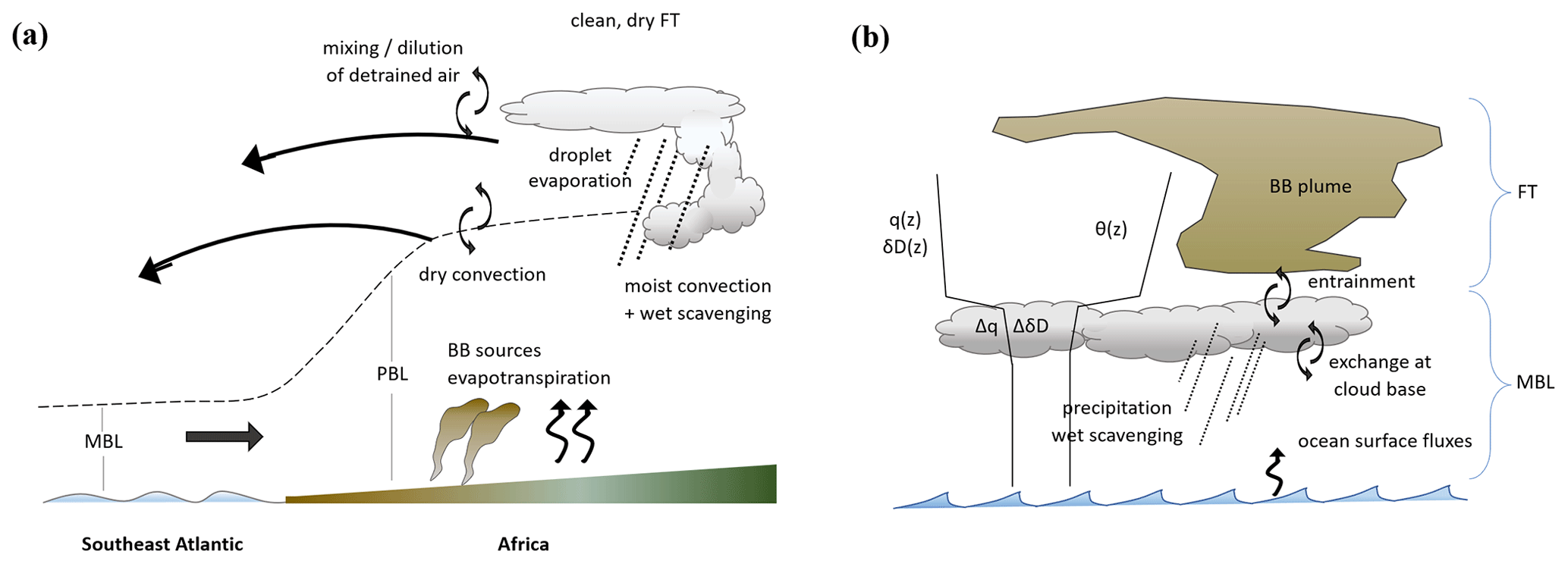
Figure 1(a) Regional moisture and aerosol transport associated with BBA plumes in the central African and southeast Atlantic regions before FT sampling during ORACLES. Processes expected to alter moisture, isotope ratios, and aerosol concentrations are shown. (b) Stratocumulus-topped marine boundary layer schematic, showing processes relevant to this study. Characteristic potential temperature (θ), total water (q), and ratio (δD) profiles are included.
Regression of the isotope data onto a simple model of convective detrainment is used to develop a metric of total precipitation for the in situ measurements; this is then compared to an aerosol metric of black carbon scavenging also derived from the in situ measurements. Next, the occurrence of entrainment mixing and precipitation in the stratocumulus-topped boundary layers is evaluated by integrating the isotopic difference between the sub-cloud layer (SCL) and cloud layer (CL) into the (q, δD) phase space framework. Correlation between processes diagnosed with the isotope ratios and variation in SCL aerosol abundance is also assessed.
Section 2 covers the ORACLES sampling region, data, and basic isotope theory. Section 3 first presents the FT analysis of precipitation histories and BC scavenging and then presents the case of the stratocumulus-topped MBL to test the degree to which the isotopic signals can detect recent precipitation (e.g., before the signal is removed by subsequent boundary layer mixing) in that very different hydrological setting. Section 4 provides a discussion of the results, and Sect. 5 provides final remarks.
2.1 ORACLES sampling region
An extensive overview of the ORACLES project is presented by Redemann et al. (2021). Aspects of the project and ORACLES measurements relevant to this study are outlined here. In situ sampling aboard the NASA P-3 Orion aircraft covered the southeast Atlantic MBL and lower FT during periods of high aerosol loading. The high BBA concentrations in the Southern Hemisphere spring are due to BBA-loaded air in the African planetary boundary layer being carried out over the southeast Atlantic by lower-FT easterly flow (Garstang et al., 1996; Adebiyi and Zuidema, 2016). This air settles over the southeast Atlantic cloud deck due to large-scale subsidence, and that air may then entrain into the MBL. The large-scale subsidence also plays a role in the strong-inversion-topped MBLs of the region, which transition to cumulus-coupled MBLs toward the Equator as sea surface temperatures (SSTs) increase (Wood, 2012, and references therein).
Sampling flight tracks are shown in Fig. 2. Sampling took place over three intensive observation periods (IOPs): 31 August–25 September 2016 (14 flights), 12 August–2 September 2017 (12 flights), and 27 September–23 October 2018 (13 flights). Flights were typically every 2–3 d, 7–9 h in duration, and within 07:00 to 17:30 LT. Vertical profiles spanned the altitude range 100 m to 7 km, covering the MBL and the region of the FT where biomass burning plumes were present.
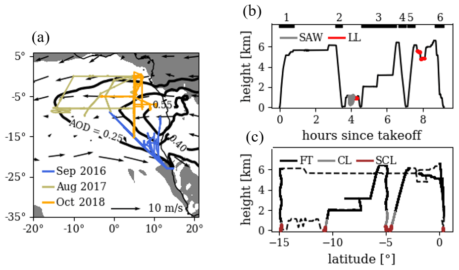
Figure 2(a) ORACLES P-3 Orion flight tracks for the three IOPs. The majority of the 2017 and 2018 IOP flight tracks are co-located geographically (blue north–south track near longitude 5∘ W). The September 2016 MERRA-2 monthly mean aerosol optical depth (black contours) and 500 hPa winds (arrows) between latitudes 25∘ S and 8∘ N are shown. Shading indicates where the September 2016 MERRA-2 monthly mean 500 hPa vertical velocity is in an upward direction. Aerosol optical depth, 500 hPa winds, and 500 hPa vertical velocity are qualitatively similar for the August 2017 and October 2018 observation periods. (b) P-3 height vs. time for the flight on 24 August 2017. In-cloud level legs (red) and sawtooth patterns (gray) are highlighted. Black bars with numbers on top indicate manually identified vertical profiles. (c) P-3 height vs. latitude, with SCL, CL, and FT regions distinguished using the vertical profiles in the top panel and the methods in Sect. 2.3.
2.2 P-3 variables used
The total water mixing ratio (q) and heavy isotope ratio were measured with the Water Isotope System for Precipitation and Entrainment Research (WISPER) instrument package, which centered on two Picarro isotopic gas analyzers (models L-2120fxi and L-2120i). The isotope ratios are reported in delta notation and the deviation of RD from that of Vienna Standard Mean Ocean Water: ). A detailed description of those data and calibration methods is given by Henze et al. (2022). Potential temperature (θ) was computed from measurements of temperature (T, Rosemount 102-type non-deiced probe) and static and dynamic (ram) pressures. Refractory black carbon (rBC) and carbon monoxide (CO) are used as indicators of BBA loading in this study. rBC concentration from 53 to 524 nm mass equivalent diameter and adjusted to standard temperature and pressure was measured using a Droplet Measurement Technologies single-particle soot photometer (Stephens et al., 2003; Schwarz et al., 2006). CO concentrations were measured by an ABB–Los Gatos Research analyzer (Liu et al., 2017). Cloud condensation nuclei (CCN) concentrations at 0.3 % supersaturation were measured by a Droplet Measurement Technologies CCN-100 continuous-flow streamwise thermal-gradient CCN chamber (Roberts and Nenes, 2005). Sub-cloud CCN measurements were used to estimate the total quantity of hygroscopic aerosols present in sampled MBLs. Measurements for q, δD, rBC, and CCN were sampled from a forward-facing solid diffuser inlet outside the P-3 cabin in front of the wing (McNaughton et al., 2007), operated by the Hawaii Group for Environmental Aerosol Research and maintained at near-isokinetic flow. CO measurements were made from a rear-facing Rosemount inlet probe.
2.3 SCL, CL, and FT identification in vertical profiles
For each flight, time intervals of vertical profiles were flagged manually. To maximize the number of data used in this study, profiles were liberally identified as any flight segment with a progressively upward or downward trajectory from near the surface (100–200 m) to at least 2500 m (e.g., Fig. 2). For each profile, vertical profiles of T, θ, and relative humidity (RH) averaged into 50 m vertical bins were used to identify the well-mixed layer top and MBL capping inversion bottom as described below. Data below the well-mixed layer top are flagged as SCL, data between the mixed layer top and inversion bottom are flagged as CL, and data above the inversion are flagged as FT. For the FT analysis, it was desired to highlight hydrologic histories of distinct air masses from the African continent (e.g., different BBA plumes), rather than any subsequent mixing between them, as they advect westward to the southeast Atlantic. Therefore, once FT segments of each profile were identified, the portions of those segments determined to be distinct air masses were isolated (rather than intermediary mixtures between them) and used for the analysis in Sect. 3.2. This was done using a pseudo-conservative variable approach described in Appendix B.
Vertical profiles of T, θ, and RH were chosen over liquid water content to flag the CL since the algorithm would also capture profiles through CLs with broken clouds, where by chance the P-3 avoided clouds during vertical ascent or descent. Mixed layer tops were roughly taken to be the height at which θ increased by 0.2 K from its 100–300 m mean. A potentially more rigorous identification of cloud base using lifting condensation levels was not used since data below 100 m were not always available. The MBLs in the study region were almost always characterized by a capping temperature inversion and a peak in RH at their top. Inversion bottoms were identified as the highest altitude below 2.5 km where a temperature minimum coincided with an RH maximum to within 150 m. The temperature minimum relative peak had to be at least 1 K and occur within a vertical region of 400 m or less. The RH absolute peak had to be greater than 80 % and occur within a vertical region of 300 m or less. Figure 2 shows an example flight using the above methods to identify the SCL, CL, and FT. Using this method, the majority of data are flagged as one of the three regions and are able to be used for analysis.
2.4 Cloud layer modules
Most flights involved modules to directly target the CL. These included (1) level legs through the cloud layer at a single altitude (LLs), typically lasting 5–15 min, and (2) sawtooth patterns through cloud layer (SAWs), also typically 5–15 min, where individual saw teeth spanned the full vertical extent of the cloud layer (Fig. 2). Both LL and SAW modules were previously flagged (e.g., Diamond et al., 2018). Where available, these modules are preferred over the CL flagging in Sect. 2.3. For LLs, data were averaged into 3 min blocks. At an aircraft horizontal speed of 130 m s−1, each block represents almost 25 km of horizontal distance, which is half the horizontal grid spacing for higher-resolution general circulation model (GCM) simulations. SAW patterns included periodic portions above and below the CL. To ensure only the CL portions are used, times where RH drops below 99 % are discarded. The remaining data are averaged into 3 min blocks. Only LLs and SAWs below 2.5 km are used.
2.5 Analysis of air mass hydrologic histories using humidity–isotope pairs
The δD of an air mass relative to its water vapor mixing ratio, q, will assume different relationships depending on the hydrologic processes the air mass experiences. Probability distribution functions (PDFs) in (q, δD) space can be compared to theoretical curves (e.g., Fig. 3) to constrain these processes. A survey discussion on the theory is presented in Noone (2012) (note that “q” in Noone, 2012, denotes water vapor, while here it denotes total water). Some key components are presented here to facilitate discussion below.
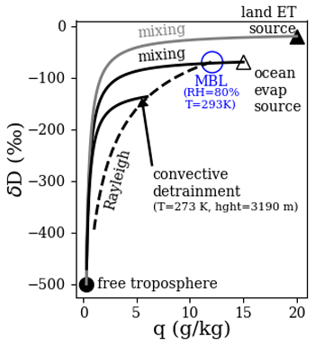
Figure 3Theoretical trajectories in (q, δD) space. Equations to generate curves were taken from Noone (2012).
Figure 3 shows the (q, δD) value of asymptotic end-members for dry FT air and pure surface evaporation from land and ocean sources. Land surface evapotranspiration (ET) may have higher δD values than ocean evaporation since transpiration does not fractionate heavy isotopes. The mixing trajectories (black, gray) show the (q, δD) relationship for air where moisture from the respective evaporation source is diluted with FT air to varying degrees. In general, air that has not experienced condensation processes may be modeled as a mixture of two or all of these end-members. The blue circle in Fig. 3 shows an example MBL placement on the mixing line assuming 80 % relative humidity with respect to a sea surface temperature of 293 K (alternatively, the blue circle could represent planetary boundary layer air over the African continent). Further entrainment of FT air into the MBL (or conversely detrainment of MBL air into the FT) would continue along the mixing trajectory. On the other hand, precipitation preferentially removes heavy isotopes, resulting in a steeper trajectory. The dashed black curve in Fig. 3 shows the extreme case of 100 % condensate removal (Rayleigh process).
In the absence of rain droplet re-evaporation, the mixing and Rayleigh processes are limiting cases that bound the region of (q, δD) space in which we expect measurements to lie. If data lie directly on the mixing curve, we hypothesize that mixing was the primary process in the recent history of the sampled air (and likewise for Rayleigh). If data lie between the curves, then the air has a more complex history. In this study, we assume that the most frequent hydrologic history occurring for the BBA-laden air is that of a convective plume model with no entrainment and 100 % precipitation efficiency (e.g., Rayleigh), which detrains at various altitudes. A convecting air mass undergoing a Rayleigh process would first follow the dashed curve from the blue circle but then be diverted along the “convective detrainment” mixing curve (solid line) upon reaching a detrainment level, when the air mass begins to dilute with FT air. We use this model to estimate total precipitation amounts in sampled FT air based on their in situ (q, δD) values (as described further in Sect. 3.3 and Fig. 9).
To support our use of the above convective detraining plume, we also compare temperature and altitude measurements from the P-3 to detrainment altitudes and temperatures estimated from the in situ (q, δD) values and our model (Sect. 3.2). The algorithm used has the following features: (1) values of surface q, T, and elevation (e.g., starting values for air lying at the blue circle in Fig. 3) are estimated from Modern-Era Retrospective analysis for Research and Applications, Version 2 (MERRA-2; Global Modeling and Assimilation Office, 2015a, b), reanalysis and used as initial conditions. (2) A temperature profile is computed from these surface values, assuming a dry adiabatic lapse rate up to a lifting condensation level and a moist lapse rate above. (3) For each q value along the Rayleigh trajectory, a dew point is calculated as the detrainment temperature and the height at which the dew point intersects the temperature profile is the detrainment height. Figure 3 shows a characteristic case with the dew point and height from this computation for the example MBL undergoing convection and detraining at q=6 g kg−1.
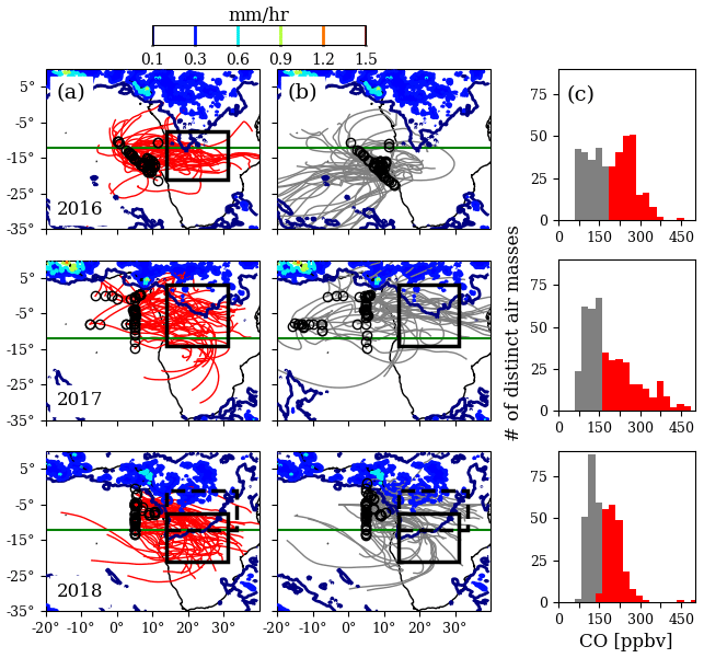
Figure 4HYSPLIT back trajectories for distinct FT air masses (identified using the methods in Appendix B) with in situ CO greater than the median (a) vs. less than the median (b). CO histograms are also shown (c). Back trajectories are shown for the September 2016 (top row), August 2017 (middle), and October 2018 (bottom) IOPs. Open black circles mark trajectory end points – the locations of P-3 in situ sampling. Overlain are NASA Global Precipitation Measurement (GPM) satellite monthly mean rainfall maps for September 2016, August 2017, and October 2018. Boxed regions mark areas over which mean MERRA-2 and isoCAM5 values were taken for calculations discussed in the main text and outlined in Table 2. The green line at 12∘ S is a visual reference. Median FT CO values for the 2016, 2017, and 2018 sampling periods were 200, 162, and 157 ppbv.
3.1 FT rainfall and evapotranspiration histories from satellite data
One objective of this study is to build a characterization of rainfall and evapotranspiration histories for FT air sampled during ORACLES using the humidity and isotopic data. For comparison, a characterization using air mass back trajectories and satellite products of monthly mean rainfall and evapotranspiration is also developed. The goal of this additional characterization is to provide a rough idea of the relative differences in precipitation and evapotranspiration which air experienced (on average) across sampling periods and across BBA concentrations. For this, 6 d back trajectories were computed with HYSPLIT (Draxler and Hess, 1997; Draxler, 1999; Warner, 2018) via the PySPLIT Python module (Warner, 2018) for FT air masses sampled by the P-3 (HYSPLIT runs used Global Data Assimilation System output on pressure levels at resolution and 3 h frequency and outputs air parcel positions at 1 h frequency). Figure 4 shows the trajectories separated by sampling period and BBA-loading histories inferred from their in situ CO concentrations. Air masses where the in situ CO concentrations were higher vs. lower than the FT median for that sampling period are referred to hereafter as high BBA vs. low BBA, respectively. It is noteworthy that a large fraction of the “low-BBA” air in the FT had CO concentrations double that typically measured in the SCL during the campaign (not shown).
For 2016, high BBA originates from the highest latitudes out of the 3 years. For 2017, both high-BBA air and low-BBA air originate further north and their latitudes tend to overlap. For 2018, the low-BBA trajectories are on average displaced 3∘ north of the high-BBA trajectories, toward regions of higher rainfall. The high-BBA air originates from a region similar to that of 2016, but whereas the 2016 high-BBA air flows west off the continent, the 2018 high-BBA air tends to flow northwest. The low-BBA air in 2016 is distinct as it often originated from higher latitudes of the Atlantic Ocean.
Figure 5 provides a first coarse assessment of the possibility of precipitation formation underway across the air mass groups in Fig. 4. It shows PDFs of monthly mean rainfall values along the back trajectories for each group, and distinct differences are apparent. In 2016, high-BBA trajectories show the lowest monthly mean rainfall. The frequency along 2016 trajectories where satellite GPM monthly mean precipitation rates are greater than 0.25 mm h−1 is an order of magnitude less than that for the other 2 years. For 2017, there is no significant difference in the PDFs for high BBA vs. low BBA, while in 2018 the low-BBA trajectories are 2× to 3× more likely than high BBA to pass over regions with precipitation >0.25 mm h−1. As will be shown further below, this characterization aligns with conclusions drawn from the isotope analysis. However, two sources of uncertainty in this first characterization are acknowledged: first, it is not clear if precipitation did really form at the time of the air mass overpass over a given region, and second, it is not clear if the air mass being tracked is really the one involved in precipitation formation.
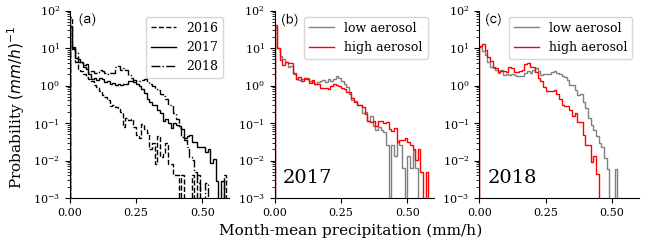
Figure 5Probability distributions of GPM monthly mean rainfall along FT back trajectories in Fig. 4. Only the portions of the trajectories over the African continent were used, defined roughly as any portion of the trajectory east of 10∘ E. Distributions between IOPs (a) and between high- vs. low-BBA air for the 2017 IOP (b) and 2018 IOP (c) are compared.
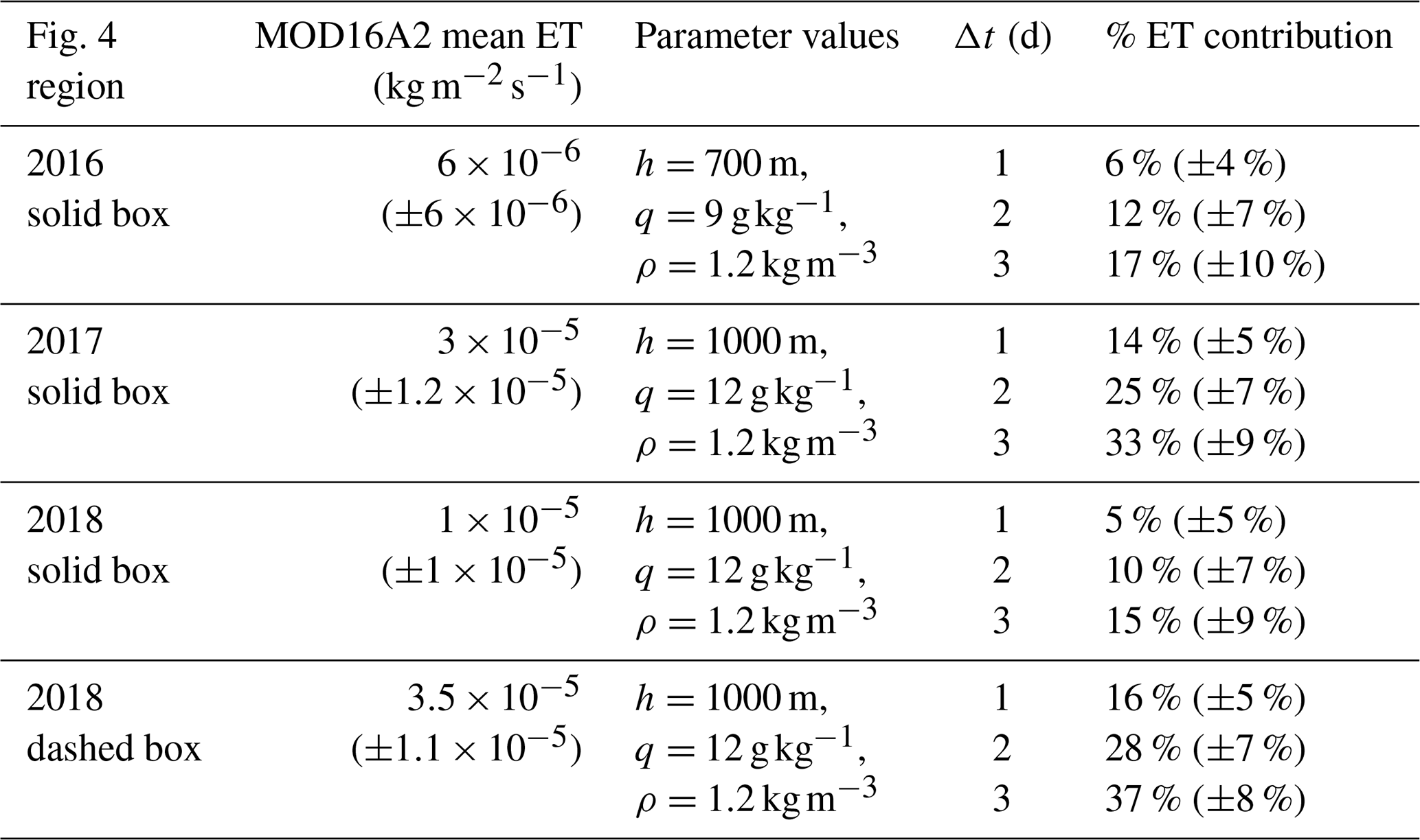
In addition to precipitation, there is variation in mean evapotranspiration (ET) in the regions from which the trajectories originate. Because ET contribution can alter the isotopic content of an air mass, its expected fraction of moisture contribution for each sampling period was estimated using a back-of-the-envelope calculation outlined in Appendix A and the MODIS Terra Version 6 Evapotranspiration/Latent Heat Flux product (MOD16A2), taking the mean and standard deviation over the boxed regions (regions bound by solid and dashed black squares) of Fig. 4. The results are shown in Table 1 and show expected ET contributions of roughly 5 %–15 % at higher latitudes and 15 %–30 % for central Africa.
Table 1Estimated ET contribution to African planetary boundary layer moisture for each ORACLES sampling period, using a back-of-the-envelope calculation (Appendix A).
3.2 FT rainfall and evapotranspiration histories from in situ humidity and isotope ratio analysis
The grouping scheme in Sect. 3.1 (by IOP and BBA-loading history) is used to categorize the in situ data to determine if similar distinctions in their precipitation and evapotranspiration histories are derived using a (q, δD) space analysis (Figs. 6–8). The asymptotic end-members and theoretical curves reviewed in Sect. 2.5 are estimated and plotted in Figs. 6–8 for each sampling period. The symbols and curves for each quantity and process match those used in Fig. 3. Table 2 summarizes their computation. Some of the end-members require estimations of near-surface values over either the ocean or the African continent, as detailed in Table 2. Near-surface temperatures and water mixing ratios were estimated using monthly mean 10 m values from MERRA-2. The δD of near-surface air over Africa is taken from output of the isotopic version of the Community Atmospheric Model simulations (isoCAM5; Nusbaumer et al., 2017), which were run for the ORACLES time period (2016–2018) and nudged with the MERRA-2 winds in a configuration very similar to that described by Fiorella et al. (2021). FT air masses are split into high-BBA (red) vs. low-BBA (gray) as in Sect. 3.1. Data for high-BBA vs. low-BBA air in Figs. 6–8 are plotted as joint probability distributions (PDFs) of (q, δD), derived using a Gaussian kernel density estimation. SCL data are plotted in blue after 60 s averaging. Horizontally, the SCL data on average fall between 65 %–80 % RH with respect to mean SST, which is reasonable. A further comparison of the SCL data with theory is provided in Appendix C. In short, the agreement between the measurements and simple theory is robust enough to provide an anchor point for the measurements and the analyses which utilize them.
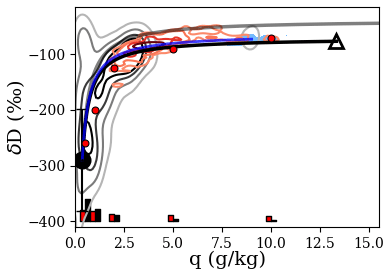
Figure 6(q, δD) PDFs for distinct FT air masses identified from vertical profiles during the September 2016 sampling period. The high-BBA data are shown in red (n=206) and low-BBA data (n=209) in gray. PDFs are expressed as cumulative probability distributions – the contours enclose 25 %, 50 %, 75 %, and 90 % of the data. The light-blue-shaded region encloses all SCL data, averaged into 30 s bins (n=203). The open triangle, large filled circle, solid black curve, and solid gray curve are analogous to those in Fig. 3 and are computed as outlined in Table 2. The blue curve is a mixing curve with moist end-member centered on the SCL data. Precisions (black bars) and accuracies (red bars) are given near the bottom, where each set of bars corresponds to the small red circle vertically above it.
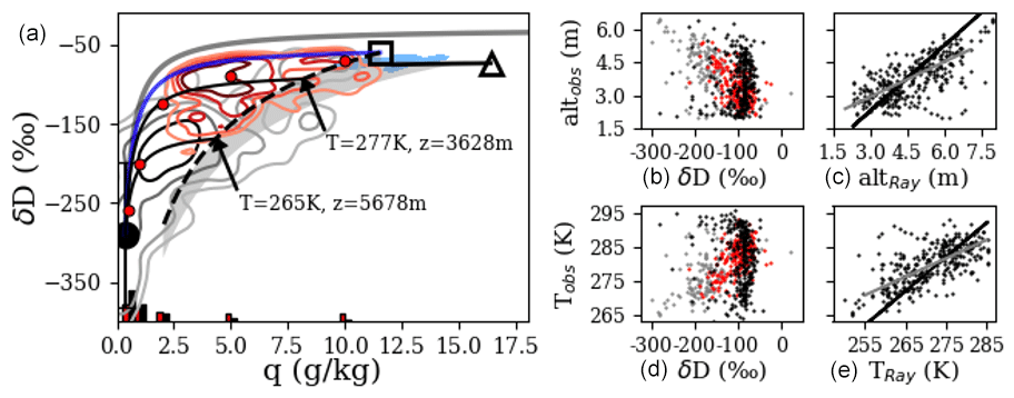
Figure 7(a) Similar to Fig. 6 but for the ORACLES 2017 sampling period. Red PDF (n=218), gray PDF (n=217), blue-shaded region (n=902), open triangle with black line segment, and gray and blue curves are as in Fig. 6. The open square represents the mean MBL adjusted for the estimated ET contribution as described in Sect. 3.1. The solid blue curve is a mixing model. Thin black curves (solid) from the Rayleigh curve (dashed) are detrainment mixing models as described in Sect. 2.5. The light-gray-shaded region bounds Rayleigh processes for all measured SCL initial values. (b, d) δD vs. height and temperature for 2017 (red, gray) and 2016 (black) data. (c, e) Observed heights and temperatures vs. those estimated using the Rayleigh model as detailed in Sect. 2.5, along with best-fit (gray) and 1:1 (black) lines.
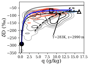
Figure 8Similar to Fig. 7 but for the ORACLES 2018 sampling period. All symbols and curves are analogous to those in Fig. 7. n=200, 200, and 780 for the red PDF, gray PDF, and blue-shaded regions, respectively. The open square near the red PDF is the point along the blue curve where q is equal to its mean MERRA-2 10 m value over the solid boxed region of Fig. 4.
Table 2Methods for computing theoretical asymptotic end-members and curves for Figs. 6–8.

The blue mixing curves in Figs. 6–8 use a combination of ORACLES in situ and MERRA-2 datasets along with the evapotranspiration estimations to provide more observationally constrained moist mixing end-members. For the 2016 IOP where ET is thought to be minimal, the mixing curve simply starts at the mean SCL (q, δD) values. For the 2017 IOP, ET contribution is estimated as 25 %. The open box in Fig. 7 represents a 75 %25 % mixture of the mean ORACLES SCL and a (q, δD) point taken from mean 10 m values derived from MERRA-2 and isoCAM5 simulations 10 m over the boxed region in Fig. 4 for 2017. It is taken as the moist end-member for the blue curve. The dashed boxed in Fig. 8 for the 2018 IOP is an analogous 75 %25 % mixture for the dashed box in Fig. 4. The solid box is provided mostly for reference and is the point along the blue curve where q reaches its MERRA-2 10 m value over the 2018 solid box in Fig. 4.
While the majority of 2016 high-BBA data can be described by dilution of high-humidity continental air with clean FT air (the blue mixing curve), the 2017 data fall well below this curve and require more analysis. The assumed model here is a detraining convective plume discussed in Sect. 2.5. Assuming an ascending parcel model following a Rayleigh process, q and δD would fall monotonically with height as water in the parcel condensed and precipitated out. Detrained air at a specific height would have a characteristic δD, and subsequent mixing with ambient dry air would alter δD relatively little (by less than 20 ‰ until the air reached about 2 g kg−1 humidity). If Rayleigh distillation followed by detrainment into dry air is in fact the primary process for the 2017 air parcels, one expectation is that δD and altitude would have good correlation. For the 2017 IOP, a correlation of −0.67 is found between δD and altitude, with δD decreasing at a mean rate of −35 ‰ km−1. In comparison, 0.05 correlation is found for the 2016 IOP despite similar sampling altitudes. Further, using the method outlined in Sect. 2.5, detrainment heights and temperatures from the Rayleigh trajectory are estimated. The best-fit lines (r of 0.68 for each) have slopes of 0.54 (Fig. 7).
For the 2018 IOP, the high-BBA air lobe falls along a mixing line with evidence of ET contribution (Fig. 8), but the PDF extends downward and is bound from below by a detrainment curve at 3600 m. The main low-BBA PDF lobe falls near a Rayleigh path, even extending below (the majority of the signal lying below the Rayleigh curve is due to air sampled below 3000 m). An estimation of altitude and temperature was performed using the Rayleigh model separately for the high- vs. low-BBA data. Correlations of 0.5 with observed values were found for each group. The low-BBA air has best-fit slopes of 0.48 and 0.51 for altitude and temperature. The high-BBA air has best-fit slopes of 0.71 and 0.86. δD decreases with altitude by 19 ‰ and 12 ‰ km−1 for the low- and high-BBA groups, respectively.
3.3 Evidence of BC scavenging from combined BC CO and (q, δD) measurements
Black carbon can serve as CCN and be permanently removed via precipitation. Carbon monoxide, on the other hand, has a low solubility in water and therefore is not altered significantly by clouds. Consequently, scavenging of BC by precipitation should cause the ratio to decrease (e.g., Liu et al., 2020). The FT (q, δD) diagrams for the 2017 and 2018 IOPs show that air masses sampled had a variety of integrated precipitation amounts, providing an approach to test for evidence of BC scavenging (2016 was not used because there is minimal occurrence of precipitation). Unlike for the previous section, where distinct air masses were isolated in order to highlight the primary hydrologic processes occurring, all data that likely originate from the African planetary boundary layer are used here. The motivation is to diagnose the influence of scavenging on BC concentrations for an arbitrary parcel of air. FT data were averaged into 60 s blocks and data with CO less than 100 ppbv were discarded, as they reflect air of marine origin.
Figure 9 shows clear gradients in coloring for (q, δD) space. If one uses the simple detraining convective plume model (outlined at the end of Sect. 2.5) to interpret the joint (q, δD) data, then the decreases with increased precipitation amount, which would be expected for scavenging. Because the detrainment mixing curve has little δD variability for q>2 g kg−1, the boxed regions depicted in Fig. 9 correspond roughly to relatively low, moderate, and high precipitation amounts. PDFs of for these three regions (Fig. 10a and b) separate with statistical significance (at α=0.05 using a t test) for both the 2017 and the 2018 IOPs. For the 2017 IOP the PDF means are 9.1, 5.9, and 3.9 . For 2018, the means are 5.1, 3.4, and 1.5 . As a control, the data separated by relatively low, moderate, and high values of q (bounds of (2,5), (5,8), and (8,11) g kg−1, respectively) show no statistically significant separation.
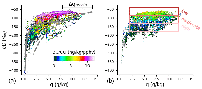
Figure 9(q, δD) diagrams for 2017 (a) and 2018 (b) IOPs, colored by rBCCO. Gray lines show schematically the regression of the detraining convective plume model onto a sample data point (filled black circle) and the estimated change in q due to precipitation. Rectangles (shades of red) show the approximation of this model applied in Fig. 10 to group a subset of the data into low, moderate, and high precipitation amounts.
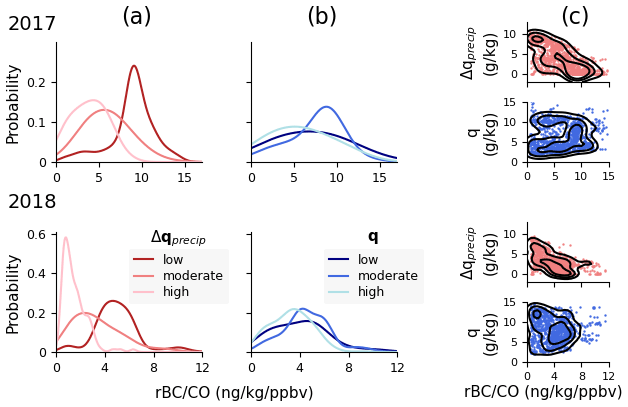
Figure 10Evidence for BC scavenging in FT BBA air using (q, δD) data. (a) rBC CO PDFs for low, moderate, and high Δqprecip as defined in Fig. 9, for the 2017 (top row) and 2018 (bottom) IOPs. (b) rBC CO PDFs for Fig. 9 data grouped by low, moderate, and high values of q as detailed in the main text. (c) Scatterplots of rBC CO versus Δqprecip and q, with PDF contours overlain.
The change in q due to precipitation, Δqprecip, is computed for each data point in Fig. 9 using an approximation to the convective plume model. For q>2 g k−1, we take the observed δD to be equal to that of the plume when it detrained, so Δqprecip can be approximated with the Rayleigh model as
where q0 is the estimated initial q of the plume before precipitation, the Rayleigh model inverted to predict q as a function of δD, and δDobs the observed value. This difference is intuitively similar to the “rainout fraction”, , that appears in Rayleigh calculation. The correlation between Δqprecip and is 0.71 for 2017 and 0.56 for 2018 (Fig. 10c). In comparison, the correlation between q and is 0.21 for 2017 and −0.14 for 2018 and distinctly inferior. This result suggests a quantifiable path for deriving BC scavenging coefficients using isotopic data that are unavailable from measures of water concentrations alone.
3.4 Entrainment mixing and precipitation in the stratocumulus-topped MBL
The variability in isotopic signals in the MBL is small in comparison to that in those of the FT. It was found that for MBLs sampled during ORACLES, the differences between the SCL and CL are small enough to be comparable to or less than SCL variability over the observation period and region. This range makes it more challenging to attribute variations in CL (q, δD) to specific CL processes (e.g., entrainment vs. precipitation) on an absolute scale given the measurement uncertainties. Therefore, CL (q, δD) data are plotted as deviations (Δq, ΔδD) from the mean values of the nearby sampled SCL, (q, δD)SCL, which subtracts out the SCL variations (Fig. 11). CL data are taken primarily from LL and SAW modules (processed as in Sect. 2.4). For these modules, (q, δD)SCL values were taken from temporally neighboring data below 500 m, which usually occurred within 10 min before or after the module, but in some cases ±20 min windows were necessary. CL data were taken secondarily from vertical profiles (Sect. 2.1) which did not include LL or SAW modules. For these profiles, (Δq, ΔδD) values were computed from the vertically averaged values of the SCL and CL for the respective profile. Only CL data for which the magnitude of the mean relative wind between the SCL and CL was less than 3.5 m s−1 were used to avoid noise due to large relative horizontal advection. Each block of SCL data used for computing (q, δD)SCL was also used to compute mean CCN values. Due to instrument limitations, it is necessary to use SCL rather than CL CCN measurements, but Diamond et al. (2018) showed that for the 2016 IOP, SCL CCN correlates well with CL droplet number concentration, implying a connection between the SCL and CL aerosol concentrations.
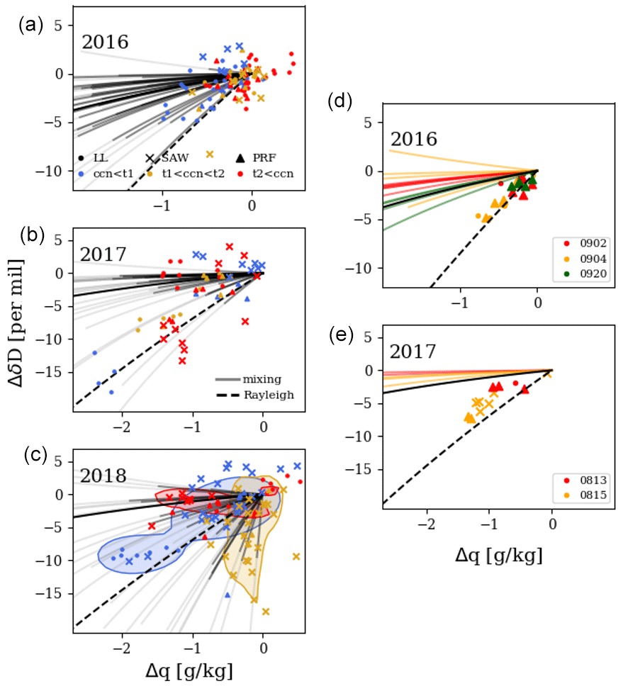
Figure 11(a–c) CL (q, δD) data expressed as deviations from the nearby SCL mean values, as described in the main text. Symbols denote the following flight module types: level leg (LL), sawtooth pattern (SAW), and vertical profiles (PRF). Colors denote tercile groups for SCL CCN (terciles listed in Table 3). (d, e) Data from several flights during the 2016 and 2017 IOPs are isolated. These data fall near a Rayleigh trajectory and cannot be explained by mixing with the overlying FT measurements for that day.
Figure 11 shows (Δq,ΔδD) diagrams colored by SCL CCN tercile groups. The CCN terciles are different for each year and are listed in Table 3. Distributions of SCL CCN are shown in Fig. 12. The solid and dashed black curves are mixing and Rayleigh curves. The end-members for the mixing curves are (q, δD)SCL and the same dry, isotopically depleted end-member used in Figs. 6–8. From here on out, this mixing trajectory is referred to as mixFT. Data which fall below mixFT are candidates for precipitation, but there are two possibilities. The first is that the CL has a recent history of precipitation. The other is that the air entraining in at CL top tends to align the data along an alternate mixing trajectory. To test this, mixing curves between (q, δD)MBL and the mean (q, δD) of the 250–500 m region above CL top (q, δD)250−500 for all vertical profiles in Sect. 2.3 are included in Fig. 11 and from here on out are referred to as mix250−500. They are expressed as (Δq,ΔδD) like the scatter points. The dark portion of the curves represent mixtures that have at most 25 % (q, δD)250−500 contribution. CLs sampled during the 2016 IOP occurred at higher latitudes in comparison to the other two IOPs, and the CLs were on average 2× to 3× shallower (Fig. 12). The majority of CLs show small deviations (Δq<0.5 g kg−1, ΔδD<4 ‰) from (q, δD)SCL. The majority of mix250−500 curves (30 out of 35) are centered on mixFT and clearly depart from the Rayleigh trajectory. Five of the curves fall closer to the Rayleigh trajectory.
Table 3Sub-cloud CCN (cm−3) terciles for the groupings in Fig. 11.
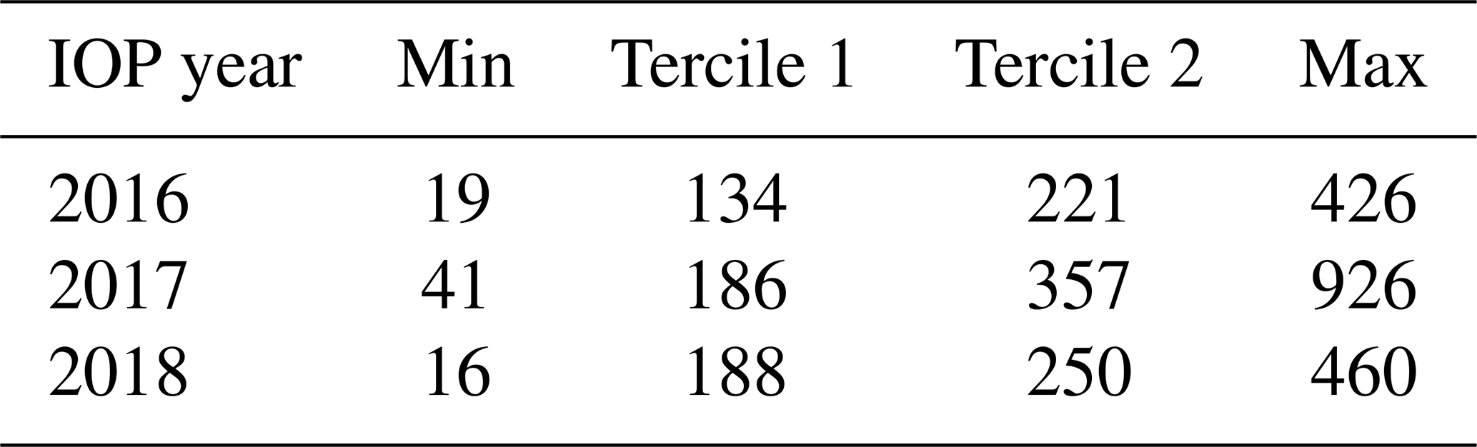
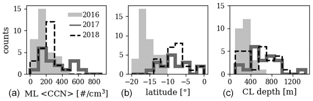
Figure 12Histograms of SCL CCN (a), CL sampling latitudes (b), and CL depths (c) for each IOP.
In comparison to the 2016 IOP, a higher proportion of 2017 IOP data deviate from (q, δD)SCL, and the standard deviation is larger. There are fewer data points shown for 2017 – since three of the flights were eastward toward Ascension Island, days where the MBL transitioned to shallow cumulus rather than a stratocumulus-topped MBL were omitted. Two-thirds of the data lie within precision of one of the mixing curves or the Rayleigh curve. The other third cannot be described by the simple models presented here. As in the 2016 IOP, the majority of mix250−500 curves are clustered about mixFT (19 of 24), while 5 pass near the Rayleigh trajectory.
For the 2018 IOP, the alternate end-member mixing curves cover a wide range of (q, δD) space rather than being clustered about mixFT, which likely explains the middle-tercile CL data (yellow). Like in the 2017 case, the data which lie near a Rayleigh trajectory with ΔδD>5 ‰ (blue cluster) could not be explained by mixing curves unless the CL contained a fraction of FT air greater than 25 % in comparison to the SCL.
4.1 FT and BBA plume hydrologic histories
Figures 4 and 5 show that FT air from the 2016 sampling period experienced the least amount of precipitation while over Africa of the three sampling periods. The in situ (q, δD) data show that in fact there are almost no signs of precipitation in the sampled high-BBA air in 2016. The PDF is enveloped from above by the theoretical ET mixing curve, suggesting ET contributions for some of the measurements, although the dominant signal is simple mixing with air close to the observed SCL values. This is interpreted as evidence of minimal ET contribution to the African planetary boundary layer air, and therefore its moisture content closely resembles the original marine source which advected onto the continent. The low-BBA data are shown for completeness, but since back trajectories suggest they often originate from the southern Atlantic rather than Africa, they are not analyzed in detail.
Both high-BBA and low-BBA data for the 2017 IOP show signs of precipitation (Fig. 7). The data are bound from above by a mixing curve with a moist end-member including 25 % ET contribution and from the right by a family of Rayleigh curves. The data support a depiction of the air mass hydrologic history as convective detrainment followed by dilution; air masses follow the Rayleigh curve during moist convection (i.e., condensation with high precipitation efficiency), then begin to detrain remaining total water at their level of neutral buoyancy, and subsequently form a diluted mixture with surrounding dry FT air. The low-BBA air is associated with convection which reached higher altitudes. A correlation of −0.67 for δD vs. height is obtained, whereas the correlation is close to 0 for the 2016 IOP despite sampling at a similar altitude range. For the 2017 IOP, detrainment heights and temperatures predicted from the Rayleigh model both have correlations of 0.67 with the observations, which is remarkable considering the simplicity of the parcel-type model used to describe the entire study period. That is, a single choice of values for surface T, q, and height; no entrainment during convection; and all condensate converted to precipitation provide a reasonable first approximation. The best-fit lines have slopes of 0.54, however. Possible reasons for why this slope is less than 1 include variation in surface conditions during convection throughout the observation period and precipitation efficiency less than unity. With respect to the latter, entrainment into an updraft would decrease δD more than expected from the Rayleigh process alone. Therefore, to achieve the same δD with only a Rayleigh process, the parcel would have to be lifted higher to compensate. Additionally, δD along detrainment curves was taken as constant to simplify the calculations. However, δD decreases by about 20 ‰ once detrained updraft air has been diluted to around 2 g kg−1, resulting in the same bias for the Rayleigh model as caused by precipitation efficiency <1.
The October 2018 sampling period comprises elements of both the 2016 and the 2017 sampling periods. The high-BBA comes from higher latitudes that are similar to those of 2016, while the low-BBA air is further north with more rainfall. However, unlike in 2016, the high-BBA air flows northwest over Africa before flowing offshore. The high-BBA air (q, δD) signal reflects this – the PDF lobe falls along a mixing line with evidence of up to 25 % ET contribution – but the distribution extends below the mixing line much more so than in 2016, bounded beneath by detrainment at 3600 m. Meanwhile, a large fraction of the low-BBA data lie near or below a Rayleigh curve, suggesting convection with a high precipitation efficiency and little subsequent mixing and potentially re-evaporation of falling droplets. Data with this signal are almost exclusively at heights below 3000 m, while data above 3000 m fall either directly on a Rayleigh curve or in the region hypothesized to be detrainment. Perhaps rain droplets falling from these higher altitudes are partially evaporating into the air below 3000 m. Such refined hydrologic history is not readily extracted without more detailed modeling.
4.2 Parsing entrainment mixing vs. precipitation in the CL and detection timescales
Cloud layer data for the 2017 and 2018 IOPs deviate further from their respective (q, δD)SCL values in comparison to the 2016 IOP. This is in line with the deeper CLs (Fig. 12) transitioning to cumulus-coupled CLs, becoming less well-mixed with the SCL, and experiencing higher entrainment and precipitation rates. CL (q, δD) measurements for all IOPs are poorly constrained by the simple mixFT and Rayleigh models – around 50 % of data for the 2016 and 2017 IOPs lie within these models, compared to only 30 % for the 2018 IOP. For the 2018 IOP, the majority of data outside these bounds can be explained by mixing with air masses above the MBL which have varying (q, δD) values. For the 2016 and 2017 IOPs, even alternate end-member mixing cannot explain the data, and these exceptions merit further study since the fraction of the data they make up is non-negligible. One possibility is the choice of a single representative (q, δD) pair for the SCL when generating the mix250−500 curves. If either or both of q and δD for overlying air were higher than the SCL values, the resulting mixing curves could explain the data in question. Differential horizontal advection of the MBL and FT could also be a contributing factor.
Although the data show signals of local precipitation in the 2016 and 2017 IOPs, the null hypothesis that all data falling below the mixFT curve came from mix250−500 curves cannot be fully ruled out with this analysis alone. However, Fig. 11 (right column) highlights some cases where the data fall near a Rayleigh trajectory and cannot be accounted for by mixing models with overlying FT air sampled on those days. Previous work has highlighted the uncertainties involved with assuming an MBL is in significant contact with the FT air above it at the time of sampling and neglecting horizontal advection (Diamond et al., 2018). Therefore, it cannot be definitively concluded that the cloud layers sampled during the highlighted flights recently precipitated. However, these flights would be good candidates to examine with advanced modeling.
Assuming that at least some of the signal is due to precipitation, a question arises regarding the time period prior to the measurement during which the precipitation occurred. Simple bulk model studies (Schubert et al., 1979; Bretherton et al., 2010; Jones et al., 2014) estimate a thermodynamic re-equilibration timescale of a stratocumulus-topped MBL at 0.5–1 d. Therefore, at longer timescales it is assumed that any isotopic evidence due to precipitation has been “erased” by subsequent turbulent mixing, including influences from surface evaporation, and consequently any signals detected are from precipitation that occurred within the past day. Previous observational studies show stratocumulus-topped MBLs precipitate primarily at night or in the early morning hours (Burleyson et al., 2013; Leon et al., 2008; Comstock et al., 2004). It may be the case that the majority of precipitation signals detected with isotope measurements are from the morning on the same day as sampling.
4.3 (q, δD) signals and SCL CCN
By inspection, there is weak SCL CCN clustering in Fig. 11 for the 2016 IOP. The two higher-CCN-tercile groups cluster about the origin, while the lowest-CCN-tercile group extends to more negative values. If only a fraction of the signals come from mix25−500 processes, the data would indicate that aerosol loading has induced precipitation suppression. The converse could also be the case: aerosol scavenging in MBLs with previous precipitation results in lower SCL CCN. Microphysical modeling would be required to quantify the causality. Further, no clear clustering is present for the 2017 IOP, in part due to the smaller signals. Indeed, using either thermodynamic or isotopic measurements to assess cloud aerosol interactions in the MBL is not necessarily achievable with simple analytical models. As a case in point, one confounding factor could be locally enhanced entrainment due to precipitation (see, e.g., Fig. 9 in Wood, 2012), which could replenish BBAs which were scavenged.
For the 2018 IOP, a consistent explanation develops from Figs. 8 and 11 (which present the 2018 IOP FT and CL data, respectively). CL data in the groups of the middle and top SCL CCN terciles are largely clustered around mixFT or the region below the Rayleigh curve (Fig. 11, shaded regions). Of these data, the highest-tercile group is primarily along the former while the middle group is along the latter. This is consistent with the (q, δD) location of high- vs. low-BBA FT PDFs in Fig. 8 if they were to serve as the above-MBL mixing end-members. Therefore, the CL data in the middle- and top-tercile groups are likely both mixtures of SCL and FT air, with the differences in MBL CCN due to the differences in FT BBA levels. Data in the lowest-tercile cluster closer to a Rayleigh trajectory, possibly indicating local precipitation and aerosol scavenging. This self-consistency in the joint (q, δD) measurements builds a degree of confidence that CL isotopic signals can be connected to entrainment processes, and potentially precipitation, even if the connection is more detailed, as for the 2017 IOP.
This study utilizes in situ measurements taken during ORACLES over three IOPs across 3 years in the Southern Hemisphere late-winter period (August–October), with 39 flights and in total ∼312 h of measurements. The FT air mass histories are deduced using the process-based expectation of variations in (q, δD) space, described by simple analytical models, in combination with several other data sources (satellite, reanalysis, and GCM output). The graphical framework is convenient to develop qualitative (and potentially quantitative) estimates of moisture contributions from different processes along the atmospheric transport pathways of water vapor (e.g., fraction of moisture from ET and convective detrainment heights). The analysis partitions air masses into those which enter the FT via dry convection and vertical mixing vs. via convection accompanied by cloud formation and precipitation. In 2016 the BBA air entered into the FT almost entirely by vertical mixing, likely exported latterly from the continental planetary boundary layer, with dilution of FT air aloft. In contrast, in 2017 both high- and low-BBA FT air are primarily associated with convective detrainment, where measurements provide evidence that low-BBA air is associated with convective detrainment at higher altitudes. In 2018, the lower-BBA air experienced precipitation. In fact, most measurements indicate that direct convection (e.g., minimal dilution after detrainment) was sampled, and considerable fractions of low-BBA air lying below the Rayleigh curve are indicative of partial re-evaporation of falling raindrops. High-BBA air for 2018 shows a combination of mixing with ET contribution and convective detrainment, which is important to the hydrologic picture.
There is strong correlation between (q, δD) evidence of precipitation and evidence of scavenging in FT BBA plumes. As a control, along mixing trajectories shows little consistency. Change in q due to precipitation, Δqprecip, derived from the isotopic data is correlated with , 0.71 for 2017 and 0.56 for 2018. This diagnostic partitioning cannot be achieved with the humidity measurements alone – correlation between q and is 0.21 for 2017 and −0.14 for 2018. Some previous studies on black carbon scavenging use BC properties and ratios in cloud droplets (Ohata et al., 2016; Liu et al., 2020; Twohy et al., 2021) to assess scavenging mechanisms and coefficients. However, they are unable to link their results to the integrated precipitation amount. Here, because the isotopic data serve as an independent measure of integrated precipitation (rather than a precipitation rate as with radar), they may provide a unique and complementary way of determining BC scavenging in the FT. For the analysis presented here, BC concentrations in the African planetary boundary layer would be required to derive numerical values for the scavenging coefficient. An ideal sampling strategy would observe the (q, δD) and BC of air within and above the planetary boundary layer simultaneously measured in a Lagrangian framework, providing direct values of Δqprecip, the change in BC, and in turn a scavenging coefficient.
Next, a test of whether a (q, δD) analysis could detect recently precipitating stratocumulus MBLs was performed. An analysis utilizing relative differences between the SCL and CL was chosen due to large measurement uncertainties and lack of ocean surface δD measurements. This posed challenges since relative differences in δD between these two vertical regions tend to be small. While no strong statements on precipitation or its interaction with aerosols can be made from this study, several key conclusions are made. For all IOPs, the fact that the CL is coupled to the surface will tend to erase signals of precipitation events, or at least convolute them with other processes. From previous studies, it is inferred that the timescale at which this occurs is 0.5–1 d. However, by far the most difficult obstacle for the ORACLES dataset is the ambiguity in CL signals due to variability in (q, δD) of the entraining air. Some air masses sampled above cloud top had values that, if entrained into the CL, were capable of lowering the CL δD values toward a region of (q, δD) space that would otherwise appear as precipitation. Such air masses were observed about 14 %, 20 %, and 60 % of the time for the 2016, 2017, and 2018 IOPs, respectively. For the 2016 IOP, the data which do suggest recent precipitation are typically connected to MBLs with the lowest SCL CCN values, which could reflect aerosol scavenging. For the 2018 IOP, the CL (q, δD) data are combined with SCL CCN values and the FT (q, δD) diagram to develop a hypothesis for the regional conditions: the middle and highest CCN values in the MBL are likely connected with variation in aerosol levels of entraining air, while the lowest MBL CCN values are the result of local precipitation. It may be the case that simply looking at relative differences between the SCL and CL does not produce an adequate signal but that an MBL which experiences precipitation, even with subsequent mixing, can produce a column-averaged δD lower than that for an MBL with only mixing and no precipitation. More complex models appear necessary to obtain constraints on precipitation versus entrainment mixing and their effects on MBL aerosol concentration. Nonetheless, this study provides evidence that such models could potentially produce these constraints, when coupled with targeted observations, and are worth pursuing further.
Because ET contribution can alter the isotopic content of an air mass, its expected fraction of moisture contribution for each sampling period was estimated using the following back-of-the-envelope calculation. For a marine boundary layer column with cross-sectional area 1 m2, the total mass of water in the column , where h is the height of the column and qa and ρa are the column-averaged specific humidity and air density. If the column advects onto land, then the total mass of water added to the column by ET over some time Δt is , where ET is the mean net evapotranspiration in units of . Therefore, assuming negligible input of water from free-tropospheric entrainment, the fraction of ET contribution is . ET is estimated using the MODIS Terra Version 6 Evapotranspiration/Latent Heat Flux product (MOD16A2), taking the mean and standard deviation over the boxed regions of Fig. 4.
For the FT analysis, it was desired to highlight hydrologic histories of distinct air masses from the African continent (e.g., different BBA plumes), rather than any subsequent mixing between them, as they advect westward to the southeast Atlantic. Therefore, distinct FT air masses in each vertical profile were identified using a pseudo-conservative variable approach to highlight the differing hydrologic histories rather than the subsequent mixtures between them. Simple two-end-member mixing processes are found as straight lines on the diagram, while curved segments signal non-conservative processes such as precipitation or more complex mixing environments (such as multiple sources or time-evolving end-members). Diagrams of q vs. equivalent potential temperature (θe) have been used before to identify regions of mixing in atmospheric profiles as well as the mixing end-members (Paluch, 1979; Betts and Albrecht, 1987). Here, instead of θe, the quantity is utilized (since the mixing ratios qHDO and q are both conserved in mixing processes, so is the linear combination qδD).
P-3 vertical profiles as identified in Sect. 2.3 were averaged into 25 m altitude bins and their trajectories in q vs. qδD space were visually broken into piecewise segments. Figure B1 shows an example of segment identification, with associated profiles of thermodynamic quantities and the BBA indicator rBC. The diagram of q vs. qδD shows a series of piecewise segments, where the corners/kinks are taken as the independent end-members (open circles). The vertical profiles show that these air masses correspond to minima/maxima in the profiles of (q, δD) and rBC or are near kinks in the θ profile, supporting the validity of this method. Although some of these air masses reside in the MBL, only the FT air masses were used.
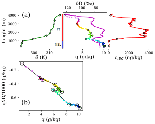
Figure B1(a) One of the P-3 vertical profiles on the 4 September 2016 flight, averaged into 25 m bins. Profiles of in situ potential temperature (green), the total water mixing ratio colored by altitude, δD (magenta), and refractory black carbon (red). (b) q vs. qδD for the profile, with the same altitude coloring as the total water profile. Open circles in (a) and (b) mark distinct air masses as outlined in Appendix B, identified visually from (b).
Figure C1 shows SCL data averaged into 60 s blocks, where the SCL was identified as in Sect. 2.3. Data below 150 m are colored by SST. SST was determined by interpolating NOAA COBE monthly mean SST satellite data to the position of the aircraft. Previous studies have been devoted to a detailed understanding of the isotopic composition of the SCL, typically using either land- or ship-based measurements (e.g., Benetti et al., 2018; Feng et al., 2019). Rather than testing those analyses in detail, the ORACLES SCL data are shown here briefly for context as a basis for the novel aspects of the aircraft profile dataset. Nonetheless, Fig. C1 includes δD predictions using the simple model of Merlivat and Jouzel (1979) (MJ79). The MJ79 model – which assumes SCL moisture comes solely from ocean evaporation – was not originally intended for regional-scale and sub-daily predictions, and its limitations in doing so have been investigated elsewhere (e.g., Jouzel and Koster, 1996; Kurita, 2013). The MJ79 model reduces SCL δD to a simple function of SST and relative humidity with respect to SST (RHS) and provides a useful reference point. For each 60 s average, the MJ79 formula was used for ocean δD values in the range of 0 ‰ to 6 ‰ for the 2017 and 2018 IOPs and in the range of 0 ‰ to 10 ‰ for 2016. The range was used to account for uncertainty in the ocean isotopic values which were not sampled during ORACLES. The upper bounds were taken by inspection of Fig. 4 in Benetti et al. (2017).
The right column of Fig. C1 provides a metric of variability in the SCL. The histograms show the difference between means of the lowermost and uppermost sampled 100 m of the SCL for each vertical profile in Sect. 2.3. The standard vertical difference is about 1 ‰ for 2016 and 2‰ for the other two IOPs. Horizontal variability is also explored. Horizontal aircraft legs below 500 m and lasting at least 3 min were averaged into 10 s blocks, and then the standard deviation of the entire leg was computed. The median horizontal standard deviations are roughly the same as the standard vertical variabilities for 2016 and 2017. For 2018, the median horizontal variability is 1.25 ‰, slightly less than the 2 ‰ vertical variability.
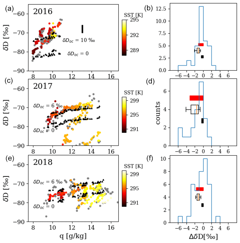
Figure C1(a, c, e) (q,δD) data in the SCL for 2016 (a), 2017 (c), and 2018 (e), averaged into 60 s blocks. Measurements below 150 m height are colored by NOAA COBE monthly mean satellite SST. Black triangles show predictions using the Merlivat and Jouzel (1979) closure assumption. The vertical black bar displayed for 2016 is the instrument standard error on an absolute scale. (b, d, f) Histograms of the difference in δD between the top- and bottommost sampled 100 m of the SCL for each vertical profile (b, 2016; d, 2017; f, 2018). Red bars are the standard deviations of the histograms. Box plots are the δD standard deviations of all P-3 horizontal legs below 500 m height and lasting at least 3 min averaged to 0.1 Hz (n=23, 22, 25 for 2016, 2017, 2018 IOPs). Black bars are 0.1 Hz instrument precisions. All standard deviations are multiplied by −1 for visuals.
The processing code can be accessed at https://doi.org/10.5281/zenodo.10252985 (Henze, 2023).
ORACLES P-3 data for each IOP can be accessed at https://doi.org/10.5067/Suborbital/ORACLES/P3/2016_V3 (ORACLES Science Team, 2020a), https://doi.org/10.5067/Suborbital/ORACLES/P3/2017_V3 (ORACLES Science Team, 2020b), and https://doi.org/10.5067/Suborbital/ORACLES/P3/2018_V3 (ORACLES Science Team, 2020c). MERRA-2 data sets used in this study can be accessed at https://doi.org/10.5067/TRD91YO9S6E7 (Global Modeling and Assimilation Office, 2015a) and https://doi.org/10.5067/XOGNBQEPLUC5 (Global Modeling and Assimilation Office, 2015b). Monthly mean precipitation data from the Global Precipitation Measurement Project can be accessed at https://doi.org/10.5067/GPM/DPRGMI/CMB/3B-MONTH/07 (see Olson, 2022). The MODIS Terra net evapotranspiration data product can be access at https://doi.org/10.5067/MODIS/MOD16A2.006 (see Running et al., 2017).
DH carried out the formal analysis and visualization and prepared the manuscript with contributions from all co-authors. DN obtained funding for the project, contributed to analysis conceptualization, and provided supervision. DT provided resources and critical guidance to place the analysis in the context of aerosol and black carbon research.
The contact author has declared that none of the authors has any competing interests.
Publisher’s note: Copernicus Publications remains neutral with regard to jurisdictional claims made in the text, published maps, institutional affiliations, or any other geographical representation in this paper. While Copernicus Publications makes every effort to include appropriate place names, the final responsibility lies with the authors.
ORACLES was a NASA Earth Venture Suborbital-2 investigation managed through the Earth System Science Pathfinder office. The authors acknowledge the financial support of the National Science Foundation (NSF).
This research has been supported by the National Science Foundation Climate and Large-scale Dynamics and Atmospheric Chemistry programs (NSF grant no. 1564670).
This paper was edited by Matthew Lebsock and reviewed by two anonymous referees.
Ackerman, A. S., Toon, O. B., Stevens, D. E., Heymsfield, A. J., Ramanathan, V., and Welton, E. J.: Reduction of tropical cloudiness by soot, Science, 288, 1042–1047, https://doi.org/10.1126/science.288.5468.1042, 2000.
Adebiyi, A. and Zuidema, P.: The Role of the Southern African Easterly Jet in Modifying the Southeast Atlantic Aerosol and Cloud Environments, Q. J. Roy. Meteor. Soc., 142, 1574–1589, https://doi.org/10.1002/qj.2765, 2016.
Albrecht, B. A.: Aerosols, cloud microphysics, and fractional cloudiness, Science, 245, 1227–1230, https://doi.org/10.1126/science.245.4923.1227, 1989.
Bailey, A., Toohey, D., and Noone, D.: Characterizing moisture exchange between the Hawaiian convective boundary layer and free troposphere using stable isotopes in water, J. Geophys. Res.-Atmos., 118, 8208–8221, https://doi.org/10.1002/jgrd.50639, 2013.
Benetti, M., Aloisi, G., Reverdin, G., Risi, C., and Seze, G.: Importance of boundary layer mixing for the isotopic composition of surface vapor over the subtropical North Atlantic Ocean, J. Geophys. Res.-Atmos., 120, 2190–2209, https://doi.org/10.1002/2014JD021947, 2015.
Benetti, M., Reverdin, G., Aloisi, G., and Sveinbjörnsdóttir, A.: Stable isotopes in surface waters of the Atlantic Ocean: Indicators of ocean-atmosphere water fluxes and oceanic mixing processes, J. Geophys. Res.-Oceans, 122, 4723–4742, https://doi.org/10.1002/2017JC012712, 2017.
Benetti, M., Lacour, J.-L., Sveinbjörnsdóttir, A. E., Aloisi, G., Reverdin, G., Risi, C., Peters, A. J., and Steen-Larsen, H. C.: A framework to study mixing processes in the marine boundary layer using water vapor isotope measurements, Geophys. Res. Lett., 45, 2524–2532, https://doi.org/10.1002/2018GL077167, 2018.
Betts, A. K. and Albrecht, B. A.: Conserved Variable Analysis of the Convective Boundary Layer Thermodynamic Structure over the Tropical Oceans, J. Atmos. Sci., 44, 83–99, https://doi.org/10.1175/1520-0469(1987)044<0083:CVAOTC>2.0.CO;2, 1987.
Bond, T. C., Doherty, S. J., Fahey, D. W., Forster, P. M., Berntsen, T., DeAngelo, B. J., Flanner, M. G., Ghan, S., Kärcher, B., Koch, D., Kinne, S., Kondo, Y., Quinn, P. K., Sarofim, M. C., Schultz, M. G., Schulz, M., Venkataraman, C., Zhang, H., Zhang, S., Bellouin, N., Guttikunda, S. K., Hopke, P. K., Jacobson, M. Z., Kaiser, J. W., Klimont, Z., Lohmann, U., Schwarz, J. P., Shindell, D., Storelvmo, T., Warren, S. G., and Zender, C. S.: Bounding the role of black carbon in the climate system: A scientific assessment, J. Geophys. Res.-Atmos., 118, 5380–5552, https://doi.org/10.1002/jgrd.50171, 2013.
Bretherton, C. S., Uchida, J., and Blossey, P. N.: Slow Manifolds and Multiple Equilibria in Stratocumulus-Capped Boundary Layers, J. Adv. Model. Earth Sy., 2, 14, https://doi.org/10.3894/JAMES.2010.2.14, 2010.
Burleyson, C. D., de Szoeke, S. P., Yuter, S. E., Wilbanks, M., and Brewer, W. A.: Ship-Based Observations of the Diurnal Cycle of Southeast Pacific Marine Stratocumulus Clouds and Precipitation, J. Atmos. Sci., 70, 3876–3894, https://doi.org/10.1175/JAS-D-13-01.1, 2013.
Chand, D., Wood, R., Anderson, T., Satheesh, S. K., and Charlson, R. J.: Satellite-derived direct radiative effect of aerosols dependent on cloud cover, Nat. Geosci., 2, 181–184, https://doi.org/10.1038/ngeo437, 2009.
Comstock, K. K., Wood, R., Yuter, S. E., and Bretherton, C. S.: Reflectivity and rain rate in and below drizzling stratocumulus, Q. J. Roy. Meteor. Soc., 130, 2891–2918, https://doi.org/10.1256/QJ.03.187, 2004.
Craig, H., Gordon, L. I., and Horibe, Y.: Isotopic exchange effects in theevaporation of water, J. Geophys. Res., 68, 5079–5087, https://doi.org/10.1029/JZ068i017p05079, 1963.
Dansgaard, W.: Stable isotopes in precipitation, Tellus, 16, 436–468, https://doi.org/10.1111/j.2153-3490.1964.tb00181.x, 1964.
Diamond, M. S., Dobracki, A., Freitag, S., Small Griswold, J. D., Heikkila, A., Howell, S. G., Kacarab, M. E., Podolske, J. R., Saide, P. E., and Wood, R.: Time-dependent entrainment of smoke presents an observational challenge for assessing aerosol–cloud interactions over the southeast Atlantic Ocean, Atmos. Chem. Phys., 18, 14623–14636, https://doi.org/10.5194/acp-18-14623-2018, 2018.
Draxler, R. R.: HYSPLIT4 user's guide. NOAA Tech. Memo. ERL ARL-230, NOAA Air Resources Laboratory, Silver Spring, MD, https://arl.noaa.gov/wp_arl/wp-content/uploads/documents/reports/arl-230.pdf (last acccess: 23 October 2023), 1999.
Draxler, R. R. and Hess, G. D.: Description of the HYSPLIT_4 modeling system. NOAA Tech. Memo. ERL ARL-224, NOAA Air Resources Laboratory, Silver Spring, MD, 24 pp., https://www.arl.noaa.gov/wp_arl/wp-content/uploads/documents/reports/arl-224.pdf (last acccess: 23 October 2023), 1997.
Feng, X., Posmentier, E. S., Sonder, L. J., and Fan, N.: Rethinking Craig and Gordon's approach to modeling isotopic compositions of marine boundary layer vapor, Atmos. Chem. Phys., 19, 4005–4024, https://doi.org/10.5194/acp-19-4005-2019, 2019.
Fiorella, R. P., Siler, N., Nusbaumer, J., and Noone, D. C.: Enhancing understanding of the hydrological cycle via pairing of process-oriented and isotope ratio tracers, J. Adv. Model. Earth Sy., 13, e2021MS002648, https://doi.org/10.1029/2021MS002648, 2021.
Galewsky, J. and Hurley, J. V.: An advection-condensation model for subtropical water vapor isotopic ratios, J. Geophys. Res., 115, D16116, https://doi.org/10.1029/2009JD013651, 2010.
Garstang, M., Tyson, P. D., Swap, R., Edwards, M., Kållberg, P., and Lindesay, J. A.: Horizontal and vertical transport of air over southern Africa, J. Geophys. Res., 101, 23721–23736, https://doi.org/10.1029/95JD00844, 1996.
Global Modeling and Assimilation Office (GMAO): MERRA-2 instU_3d_ana_Np: 3d,diurnal,Instantaneous,Pressure-Level,Analysis,Analyzed Meteorological Fields V5.12.4, Goddard Earth Sciences Data and Information Services Center (GES DISC) [data set], Greenbelt, MD, USA, https://doi.org/10.5067/TRD91YO9S6E7, 2015a.
Global Modeling and Assimilation Office (GMAO): MERRA-2 instM_2d_gas_Nx: 2d,Monthly mean,Instantaneous,Single-Level,Assimilation,Aerosol Optical Depth Analysis V5.12.4, Goddard Earth Sciences Data and Information Services Center (GES DISC) [data set], Greenbelt, MD, USA, https://doi.org/10.5067/XOGNBQEPLUC5, 2015b.
Henze, D.: Processing Code for Henze et al., ACP 2023, Version v2, Zenodo [code], https://doi.org/10.5281/zenodo.10252985, 2023.
Henze, D., Noone, D., and Toohey, D.: Aircraft measurements of water vapor heavy isotope ratios in the marine boundary layer and lower troposphere during ORACLES, Earth Syst. Sci. Data, 14, 1811–1829, https://doi.org/10.5194/essd-14-1811-2022, 2022.
Horita, J. and Wesolowski, D. J.: Liquid-vapor fractionation of oxygen and hydrogen isotopes of water from the freezing to the critical temperature, Geochim. Cosmochim. Ac., 58, 3425–3437, https://doi.org/10.1016/0016-7037(94)90096-5, 1994.
IPCC: Climate Change 2013: The Physical Science Basis. Contribution of Working Group I to the Fifth Assessment Report of the Intergovernmental Panel on Climate Change, edited by: Stocker, T. F., Qin, D., Plattner, G.-K., Tignor, M., Allen, S. K., Boschung, J., Nauels, A., Xia, Y., Bex, V., and Midgley, P. M., Cambridge University Press, Cambridge, United Kingdom and New York, NY, USA, in press, https://doi.org/10.1017/CBO9781107415324, 2013.
Jones, C. R., Bretherton, C. S., and Blossey, P. N.: Fast stratocumulus time scale in mixed layer model and large eddy simulation, J. Adv. Model. Earth Sy., 6, 206–222, https://doi.org/10.1002/2013MS000289, 2014.
Jouzel, J. and Koster, R. D.: A reconsideration of the initial conditions used for stable water isotope models, J. Geophys. Res., 101, 22933–22938, https://doi.org/10.1029/96JD02362, 1996.
Kurita, N.: Water isotopic variability in response to mesoscale convective system over the tropical ocean, J. Geophys. Res.-Atmos., 118, 10376–10390, https://doi.org/10.1002/jgrd.50754, 2013.
Latha, K. M., Badarinath, K. V. S., and Reddy, P. M.: Scavenging efficiency of rainfall on black carbon aerosols over an urban environment, Atmos. Sci. Lett., 6, 148–151, https://doi.org/10.1002/asl.108, 2005.
Leon, D. C., Wang, Z., and Liu, D.: Climatology of drizzle in marine boundary layer clouds based on 1 year of data from CloudSat and Cloud-Aerosol Lidar and Infrared Pathfinder Satellite Observations (CALIPSO), J. Geophys. Res., 113, D00A14, https://doi.org/10.1029/2008JD009835, 2008.
Liu, X., Huey, L. G., Yokelson, R. J., et al.: Airborne measurements of western U. S. wildfire emissions: Comparison with prescribed burning and air quality implications, J. Geophys. Res.-Atmos., 122, 6108–6129, https://doi.org/10.1002/2016jd026315, 2017.
Liu, D., Ding, S., Zhao, D., Hu, K., Yu, C., Hu, D., Wu, Y., Zhou, C., Tian, P., Liu, Q., Wu, Y., Zhang, J., Kong, S., Huang, M., and Ding, D.: Black carbon emission and wet scavenging from surface to the top of boundary layer over Beijing region, J. Geophys. Res.-Atmos., 125, e2020JD033096, https://doi.org/10.1029/2020JD033096, 2020.
McNaughton, C. S., Clarke, A. D., Howell, S. G., Pinkerton, M., Anderson, B., Thornhill, L., Winstead, E., Hudgins, C., Dibb, J. E., Scheuer, E., and Maring, H.: Results from the DC-8 inlet characterization experiment (DICE): Airborne versus surface sampling of mineral dust and sea salt aerosols, Aerosol Sci. Tech., 41, 136–159, https://doi.org/10.1080/02786820601118406, 2007.
Merlivat, L. and Jouzel, J.: Global climatic interpretation of the deuterium-oxygen 18 relationship for precipitation, J. Geophys. Res., 84, 5029–5033, https://doi.org/10.1029/JC084iC08p05029, 1979.
Noone, D.: Pairing Measurements of the Water Vapor Isotope Ratio with Humidity to Deduce Atmospheric Moistening and Dehydration in the Tropical Midtroposphere, J. Climate, 25, 4476–4494, https://doi.org/10.1175/JCLI-D-11-00582.1, 2012.
Noone, D., Galewsky, J., Sharp, Z. D., Worden, J., Barnes, J., Baer, D., Bailey, A., Brown, D. P., Christensen, L., Crosson, E., Dong, F., Hurley, J. V., Johnson, L. R., Strong, M., Toohey, D., Van Pelt, A., and Wright, J. S.: Properties of air mass mixing and humidity in the subtropics from measurements of the D/H isotope ratio of water vapor at the Mauna Loa Observatory, J. Geophys. Res., 116, D22113, https://doi.org/10.1029/2011JD015773, 2011.
Nusbaumer, J., Wong, T. E., Bardeen, C., and Noone, D.: Evaluating hydrological processes in the Community Atmosphere Model Version 5 (CAM5) using stable isotope ratios of water, J. Adv. Model. Earth Sy., 9, 949–977, https://doi.org/10.1002/2016MS000839, 2017.
Ohata, S., Moteki, N., Mori, T., Koike, M., and Kondo, Y.: A key process controlling the wet removal of aerosols: new observational evidence, Sci. Rep.-UK, 6, 34113, https://doi.org/10.1038/srep34113, 2016.
Olson, W.: GPM DPR and GMI (Combined Precipitation) L3 1 month 0.25 degree x 0.25 degree V07, Goddard Earth Sciences Data and Information Services Center (GES DISC) [data set], Greenbelt, MD, USA, https://doi.org/10.5067/GPM/DPRGMI/CMB/3B-MONTH/07, 2022.
ORACLES Science Team: Suite of Aerosol, Cloud, and Related Data Acquired Aboard P3 During ORACLES 2016, Version 3, NASA Ames Earth Science Project Office (ESPO) [data set], Moffett Field, CA, https://doi.org/10.5067/Suborbital/ORACLES/P3/2016_V3, 2021.
ORACLES Science Team: Suite of Aerosol, Cloud, and Related Data Acquired Aboard P3 During ORACLES 2017, Version 3, NASA Ames Earth Science Project Office (ESPO) [data set], Moffett Field, CA, https://doi.org/10.5067/Suborbital/ORACLES/P3/2017_V3, 2021.
ORACLES Science Team: Suite of Aerosol, Cloud, and Related Data Acquired Aboard P3 During ORACLES 2018, Version 3, NASA Ames Earth Science Project Office (ESPO) [data set], Moffett Field, CA, https://doi.org/10.5067/Suborbital/ORACLES/P3/2018_V3, 2021c.
Paluch, I. R.: The entrainment mechanism in Colorado cumuli, J. Atmos. Sci., 36, 2467–2478, https://doi.org/10.1175/1520-0469(1979)036<2467:TEMICC>2.0.CO;2, 1979.
Redemann, J., Wood, R., Zuidema, P., Doherty, S. J., Luna, B., LeBlanc, S. E., Diamond, M. S., Shinozuka, Y., Chang, I. Y., Ueyama, R., Pfister, L., Ryoo, J.-M., Dobracki, A. N., da Silva, A. M., Longo, K. M., Kacenelenbogen, M. S., Flynn, C. J., Pistone, K., Knox, N. M., Piketh, S. J., Haywood, J. M., Formenti, P., Mallet, M., Stier, P., Ackerman, A. S., Bauer, S. E., Fridlind, A. M., Carmichael, G. R., Saide, P. E., Ferrada, G. A., Howell, S. G., Freitag, S., Cairns, B., Holben, B. N., Knobelspiesse, K. D., Tanelli, S., L'Ecuyer, T. S., Dzambo, A. M., Sy, O. O., McFarquhar, G. M., Poellot, M. R., Gupta, S., O'Brien, J. R., Nenes, A., Kacarab, M., Wong, J. P. S., Small-Griswold, J. D., Thornhill, K. L., Noone, D., Podolske, J. R., Schmidt, K. S., Pilewskie, P., Chen, H., Cochrane, S. P., Sedlacek, A. J., Lang, T. J., Stith, E., Segal-Rozenhaimer, M., Ferrare, R. A., Burton, S. P., Hostetler, C. A., Diner, D. J., Seidel, F. C., Platnick, S. E., Myers, J. S., Meyer, K. G., Spangenberg, D. A., Maring, H., and Gao, L.: An overview of the ORACLES (ObseRvations of Aerosols above CLouds and their intEractionS) project: aerosol–cloud–radiation interactions in the southeast Atlantic basin, Atmos. Chem. Phys., 21, 1507–1563, https://doi.org/10.5194/acp-21-1507-2021, 2021.
Risi, C., Noone, D., Worden, J., Frankenberg, C., Stiller, G., Kiefer, M., Funke, B., Walker, K., Bernath, P., Schneider, M., Wunch, D., Sherlock, V., Deutscher, N., Griffith, D., Wennberg, P. O., Strong, K., Smale, D., Mahieu, E., Barthlott, S., Hase, F., García, O., Notholt, J., Warneke, T., Toon, G., Sayres, D., Bony, S., Lee, J., Brown, D., Uemura, R., and Sturm, C.: Process-evaluation of tropospheric humidity simulated by general circulation models using water vapor isotopologues: 1. Comparison between models and observations, J. Geophys. Res., 117, D05303, https://doi.org/10.1029/2011JD016621, 2012.
Roberts, G. C. and Nenes, A.: A Continuous-Flow Streamwise Thermal-Gradient CCN Chamber for Atmospheric Measurements, Aerosol Sci. Technol., 39, 206–221, https://doi.org/10.1080/027868290913988, 2005.
Running, S., Mu, Q., and Zhao, M.: MOD16A2 MODIS/Terra Net Evapotranspiration 8-Day L4 Global 500m SIN Grid V006, NASA EOSDIS Land Processes Distributed Active Archive Center [data set], https://doi.org/10.5067/MODIS/MOD16A2.006, 2017.
Schubert, W. H., Wakefield, J. S., Steiner, E. J., and Cox, S. K.: Marine stratocumulus convection. Part II: Horizontally inhomogeneous solutions, J. Atmos. Sci., 36, 1308–1324, https://doi.org/10.1175/1520-0469(1979)036<1308:MSCPIH>2.0.CO;2, 1979.
Schwarz, J. P., Gao, R. S., Fahey, D. W., Thomson, D. S., Watts, L. A., Wilson, J. C., Reeves, J. M., Darbeheshti, M., Baumgardner, D. G., Kok, G. L., Chung, S. H., Schulz, M., Hendricks, J., Lauer, A., Kärcher, B., Slowik, J. G., Rosenlof, K. H., Thompson, T. L., Langford, A. O., Loewenstein, M., and Aikin, K. C.: Single-particle measurements of midlatitude black carbon and light-scattering aerosols from the boundary layer to the lower stratosphere, J. Geophys. Res., 111, D16207, https://doi.org/10.1029/2006jd007076, 2006.
Steen-Larsen, H. C., Sveinbjörnsdottir, A. E., Jonsson, Th., Ritter, F., Bonne, J.-L., Masson-Delmotte, V., Sodemann, H., Blunier, T., Dahl-Jensen, D., and Vinther, B. M.: Moisture sources and synoptic to seasonal variability of North Atlantic water vapor isotopic composition, J. Geophys. Res.-Atmos., 120, 5757–5774, https://doi.org/10.1002/2015JD023234, 2015.
Stephens, M., Turner, N., and Sandberg, J.: Particle identification by laser-induced incandescence in a solid-state laser cavity, Appl. Optics, 42, 3726–3736, https://doi.org/10.1364/ao.42.003726, 2003.
Textor, C., Schulz, M., Guibert, S., Kinne, S., Balkanski, Y., Bauer, S., Berntsen, T., Berglen, T., Boucher, O., Chin, M., Dentener, F., Diehl, T., Easter, R., Feichter, H., Fillmore, D., Ghan, S., Ginoux, P., Gong, S., Grini, A., Hendricks, J., Horowitz, L., Huang, P., Isaksen, I., Iversen, I., Kloster, S., Koch, D., Kirkevåg, A., Kristjansson, J. E., Krol, M., Lauer, A., Lamarque, J. F., Liu, X., Montanaro, V., Myhre, G., Penner, J., Pitari, G., Reddy, S., Seland, Ø., Stier, P., Takemura, T., and Tie, X.: Analysis and quantification of the diversities of aerosol life cycles within AeroCom, Atmos. Chem. Phys., 6, 1777–1813, https://doi.org/10.5194/acp-6-1777-2006, 2006.
Tritscher, T., Jurányi, Z., Martin, M., Chirico, R., Gysel, M., Heringa, M. F., DeCarlo, P. F., Sierau, B., Prévôt, A. S. H., Weingartner, E., and Baltensperger, U.: Changes of hygroscopicity and morphology during ageing of diesel soot, Environ. Res. Lett., 6, 034026, https://doi.org/10.1088/1748-9326/6/3/034026, 2011.
Twohy, C. H., Toohey, D. W., Levin, E. J. T., DeMott, P. J., Rainwater, B., Garofalo, L. A., Pothier, M. A., Farmer, D. K., Kreidenweis, S. M., Pokhrel, R. P., Murphy, S. M., Reeves, J. M., Moore, K. A., and Fischer, E. V.: Biomass burning smoke and its influence on clouds over the western U. S., Geophys. Res. Lett., 48, e2021GL094224, https://doi.org/10.1029/2021GL094224, 2021.
van der Werf, G. R., Randerson, J. T., Giglio, L., Collatz, G. J., Mu, M., Kasibhatla, P. S., Morton, D. C., DeFries, R. S., Jin, Y., and van Leeuwen, T. T.: Global fire emissions and the contribution of deforestation, savanna, forest, agricultural, and peat fires (1997–2009), Atmos. Chem. Phys., 10, 11707–11735, https://doi.org/10.5194/acp-10-11707-2010, 2010.
Warner, M.: Introduction to PySPLIT: A Python Toolkit for NOAA ARL's HYSPLIT Model, Comput. Sci. Eng., 20, 47–62, https://doi.org/10.1109/MCSE.2017.3301549, 2018.
Wood, R.: Cancellation of aerosol indirect effects in marine stratocumulus through cloud thinning, J. Atmos. Sci., 64, 2657–2669, https://doi.org/10.1175/JAS3942.1, 2007.
Wood, R.: Stratocumulus clouds. Review paper, Mon. Weather Rev., 140, 2373–2423, 2012.
Zhang, R. Y., Khalizov, A. F., Pagels, J., Zhang, D., Xue, H. X., and McMurry, P. H.: Variability in morphology, hygroscopicity, and optical properties of soot aerosols during atmospheric processing, P. Natl. Acad. Sci. USA, 105, 10291–10296, https://doi.org/10.1073/pnas.0804860105, 2008.
Zuberi, B., Johnson, K. S., Aleks, G. K., Molina, L. T., and Laskin, A.: Hydrophilic properties of aged soot, Geophys. Res. Lett., 32, L01807, https://doi.org/10.1029/2004gl021496, 2005.
Zuidema, P., Redemann, J., Haywood, J., Wood, R., Piketh, S., Hipondoka, M., and Formenti, P.: Interactions: Smoke and Clouds above the Southeast Atlantic Upcoming Field Campaigns Probe Absorbing Aerosol's Impact on Climate, B. Am. Meteorol. Soc., 97, 1131–1135, https://doi.org/10.1175/BAMS-D-15-00082.1, 2016.
- Abstract
- Introduction
- Methods
- Results
- Discussion
- Final remarks
- Appendix A: Estimating evapotranspiration contribution to total water mass of a boundary layer column
- Appendix B: Identifying distinct FT air masses
- Appendix C: Sub-cloud layer (q, δD) values and their variances
- Code availability
- Data availability
- Author contributions
- Competing interests
- Disclaimer
- Acknowledgements
- Financial support
- Review statement
- References