the Creative Commons Attribution 4.0 License.
the Creative Commons Attribution 4.0 License.
 | 14 Dec 2023
Decreasing trends of ammonia emissions over Europe seen from remote sensing and inverse modelling
Ondřej Tichý
Sabine Eckhardt
Yves Balkanski
Didier Hauglustaine
Nikolaos Evangeliou
Ammonia (NH3), a significant precursor of particulate matter, affects not only biodiversity, ecosystems, and soil acidification but also climate and human health. In addition, its concentrations are constantly rising due to increasing feeding needs and the large use of fertilization and animal farming. Despite the significance of ammonia, its emissions are associated with large uncertainties, while its atmospheric abundance is difficult to measure. Nowadays, satellite products can effectively measure ammonia with low uncertainty and a global coverage. Here, we use satellite observations of column ammonia in combination with an inversion algorithm to derive ammonia emissions with a high resolution over Europe for the period 2013–2020. Ammonia emissions peak in northern Europe due to agricultural application and livestock management, in western Europe (industrial activity), and over Spain (pig farming). Emissions have decreased by −26 % since 2013 (from 5431 Gg in 2013 to 3994 Gg in 2020), showing that the abatement strategies adopted by the European Union have been very efficient. The slight increase (+4.4 %) in 2015 is also reproduced here and is attributed to some European countries exceeding annual emission targets. Ammonia emissions are low in winter (286 Gg) and peak in summer (563 Gg) and are dominated by the temperature-dependent volatilization of ammonia from the soil. The largest emission decreases were observed in central and eastern Europe (−38 %) and in western Europe (−37 %), while smaller decreases were recorded in northern (−17 %) and southern Europe (−7.6 %). When complemented with ground observations, modelled concentrations using the posterior emissions showed improved statistics, also following the observed seasonal trends. The posterior emissions presented here also agree well with respective estimates reported in the literature and inferred from bottom-up and top-down methodologies. These results indicate that satellite measurements combined with inverse algorithms constitute a robust tool for emission estimates and can infer the evolution of ammonia emissions over large timescales.
- Article
(5322 KB) - Full-text XML
-
Supplement
(49563 KB) - BibTeX
- EndNote


Ammonia (NH3), the only alkaline gas in the atmosphere, constitutes one of the most reactive nitrogen species. It is produced from the decomposition of urea, which is a rapid process when catalysed by enzymes (Sigurdarson et al., 2018). The main sectors contributing to its production are livestock management and wild animals (Behera et al., 2013), biomass burning and domestic coal combustion (Fowler et al., 2004; Sutton et al., 2008), volcanic eruptions (Sutton et al., 2008), and agriculture (Erisman et al., 2007). Emissions from agricultural activity and livestock management represent over 80 % of the total emissions (Crippa et al., 2020), while their regional contribution can reach 94 % (Van Damme et al., 2018).
Once emitted, it is transported over short distances and deposited to water bodies, soil, or vegetation with a typical atmospheric lifetime of a few hours (Evangeliou et al., 2021). It can then lead to eutrophication of water bodies (Stevens et al., 2010), modulate soil pH (Galloway et al., 2003), and “burn” vegetation by pulling water from the leaves (Krupa, 2003). It also reacts with the abundant atmospheric sulfuric and nitric acids (Malm, 2004) forming fine particulate matter (PM2.5) (Tsimpidi et al., 2007). While ammonia has a short atmospheric lifetime, PM2.5 resides significantly longer in the atmosphere, on the order of days to weeks (Seinfeld and Pandis, 2000), and hence is transported over longer distances. Accordingly, secondary PM2.5 can affect the Earth's radiative balance, both directly by scattering incoming radiation (Henze et al., 2012) and indirectly as cloud condensation nuclei (Abbatt et al., 2006). Its environmental effects include visibility problems and contribution to haze formation. Finally, PM2.5 affects human health as it penetrates the human respiratory system and deposits in the lungs and alveolar regions (Pope and Dockery, 2006; Pope et al., 2002), contributing to premature mortality (Lelieveld et al., 2015).
To combat secondary pollution, the European Union established a set of measures focusing on ammonia abatement, similar to the ones introduced by China (Giannakis et al., 2019). These measures aim to reduce ammonia emissions by 6 % in 2020 relative to 2005. However, the lack of spatiotemporal measurements of ammonia over Europe makes any assessment of the efficiency of these measures difficult as only bottom-up methods are used to calculate emission. These methods still show a slight increase (0.6 % yr−1) up to 2018, mostly due to increasing agricultural activities (McDuffie et al., 2020). Such bottom-up approaches rely on uncertain land use data and emission factors that are not always up to date, thus adding large errors to existing inventories.
During the last decade, satellite products have also become available to fill the gaps created by spatially disconnected ground-based measurements. Data from satellite sounders such as the Infrared Atmospheric Sounding Interferometer (IASI) (Van Damme et al., 2017), the Atmospheric Infrared Sounder (AIRS) (Warner et al., 2017), the Cross-track Infrared Sounder (CrIS) (Shephard and Cady-Pereira, 2015), the Tropospheric Emission Spectrometer (TES) (Shephard et al., 2015), and the Greenhouse Gases Observing Satellite (GOSAT) (Someya et al., 2020) are publicly available. Most of them have been validated against ground-based observations or complemented with other remote sensing products (Van Damme et al., 2015, 2018; Dammers et al., 2016, 2017, 2019; Kharol et al., 2018; Shephard et al., 2020; Whitburn et al., 2016).
Accordingly, a few studies on ammonia emission calculations have been recently published, relying on 4D-variational inversion schemes, such as in Cao et al. (2022) and Zhu et al. (2013), or process-based models (Beaudor et al., 2023; Vira et al., 2020). More recently, Sitwell et al. (2022) proposed an inversion scheme for comparison between model profiles and satellite retrievals using hybrid logarithmic and linear observation operators that attempt to choose the best method according to the particular situation. In the present study, we use direct comparisons between the CrIS ammonia retrievals and model profiles using the Least Squares with Adaptive Prior Covariance (LS-APC) algorithm (Tichý et al., 2016), which reduces the number of tuning parameters in the method significantly using a variational Bayesian approximation technique. We constrain ammonia emissions over Europe over the 2013–2020 period and validate the results against ground-based observations from EMEP (European Monitoring and Evaluation Programme, https://emep.int/mscw/, last access: 26 October 2023) (Torseth et al., 2012).
2.1 CrIS observations
To constrain ammonia emissions with inverse modelling, satellite measurements were adopted from the Cross-Track Infrared Sounder (CrIS) on board the NASA Suomi National Polar-orbiting Partnership (S-NPP) satellite, which provides atmospheric soundings with a spectral resolution of 0.625 cm−1 (Shephard et al., 2015). CrIS presents improved vertical sensitivity for ammonia closer to the surface due to the low spectral noise in the ammonia spectral region (Zavyalov et al., 2013) and the early-afternoon overpass that typically coincides with high thermal contrast, which is optimal for thermal infrared sensitivity. The CrIS Fast Physical Retrieval (CFPR) (Shephard and Cady-Pereira, 2015) retrieves ammonia profiles at 14 levels using a physics-based optimal estimation retrieval, which also provides the vertical sensitivity (averaging kernels) and an estimate of the retrieval errors (error covariance matrices) for each measurement. As peak sensitivity typically occurs in the boundary layer between 900 and 700 hPa (∼ 1 to 3 km) (Shephard et al., 2020), and the surface and total column concentrations are both highly correlated with these boundary layer retrieved levels. The total column random measurement error is estimated to be in the 10 %–15 % range, with total errors estimated to be ∼ 30 % (Shephard et al., 2020). The individual profile retrieval levels show an estimated random measurement error of 10 %–30 %, with total random error estimates increasing to 60 %–100 % due to the limited vertical resolution (1 degree of freedom of signal for CrIS ammonia). These vertical sensitivity and error output parameters are also useful for using CrIS observations in applications (e.g. data fusion and/or data assimilation, model-based emission inversions; Cao et al., 2020; Li et al., 2019) as a satellite observational operator can be generated in a robust manner. The detection limit of CrIS measurements has been calculated down to 0.3–0.5 ppbv (Shephard et al., 2020). CrIS ammonia has been evaluated against other observations over North America with the Ammonia Monitoring Network (AMoN) (Kharol et al., 2018) and against ground-based Fourier transform infrared (FTIR) spectroscopic observations (Dammers et al., 2017), showing small bias and high correlations.
Daily CrIS ammonia (version 1.6.3) was put on a grid covering all of Europe (25–75∘ N, 10∘ W–50∘ E) for the period 2013–2020 (observations with Quality_Flag ≥ 5 and thin clouds with Cloud_Flag = 3 rejected). Gridding was chosen due to the large number of observations (around 10 000 retrievals per day per vertical level), which made the calculation of source receptor matrices (SRMs) computationally inefficient. Through gridding, we limited the number of observations (and thus the number of SRMs to be calculated) to 2000 d−1 per vertical level. Sitwell et al. (2022) showed that the averaging kernels of CrIS ammonia are significant only for the lowest six levels (the upper eight have no influence on the satellite observations); therefore, we considered only these six vertical levels (∼ 1018–619 hPa). The gridding was performed by averaging the values that fall in each 0.5∘ resolution grid cell daily over the 2013–2020 period of this study. This type of gridding was selected as previous experience with inverse distance weighting interpolation of satellite observations showed overestimated results of up to 100 % (Evangeliou et al., 2021). In addition, the quality of gridding with respect to the averaging kernel of CrIS ammonia was evaluated by calculating the standard deviation of the averaged values (Fig. S1 in the Supplement). The latter shows that the kernel values within each grid cell were very similar, resulting in low gridded standard deviations and thus low bias as a result of the gridding (Fig. S1).
2.2 A priori emissions of ammonia
We used as a priori emissions for ammonia in the inversion algorithm the ones calculated from (i) the most recent version of ECLIPSEv6 (Evaluating the CLimate and Air Quality ImPacts of Short-livEd Pollutants) (Zbigniew Klimont, personal communication, 2022; Klimont et al., 2017) combined with biomass burning emissions from GFEDv4 (Global Fire Emission Dataset) (Giglio et al., 2013), hereafter referred to as EC6G4; (ii) a more traditional dataset from ECLIPSEv5, GFEDv4, and GEIA (Global Emissions InitiAtive), hereafter referred to as EGG (Bouwman et al., 1997; Giglio et al., 2013; Klimont et al., 2017); (iii) emissions calculated from IASI (Infrared Atmospheric Sounding Interferometer) and a one-dimensional box model and a modelled lifetime (Evangeliou et al., 2021), denoted as NE; and (iv) the high-resolution dataset of Van Damme et al. (2018) after applying a simple one-dimensional box model (Evangeliou et al., 2021), hereafter denoted as VD. Given the large uncertainty in ammonia emissions illustrated in Fig. 1, we calculated the average of these four priors (hereafter referred to avgEENV) to establish the a priori emissions used in this study.
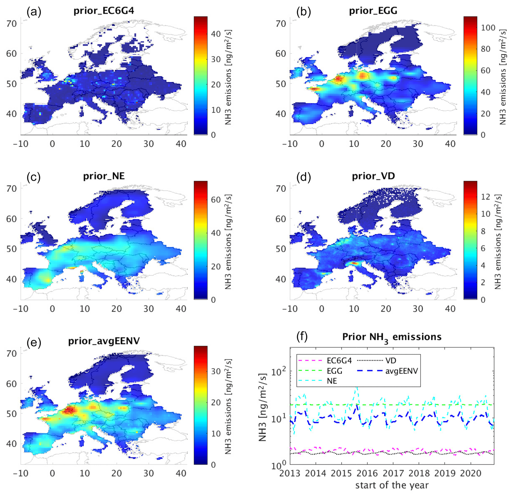
Figure 1Four ammonia prior emissions (EC6G4, EGG, NE, VD) are displayed in the first two rows. The combined prior (avgEENV) is displayed in the bottom left. The temporal variability of all five prior emissions is given in the bottom right.
2.3 Lagrangian particle dispersion model for the calculation of source receptor matrices (SRMs) of ammonia
SRMs were calculated for each grid cell over Europe (25–75∘ N, 10∘ W–50∘ E) using the Lagrangian particle dispersion model FLEXPART version 10.4 (Pisso et al., 2019), adapted to simulate ammonia. The adaptation of the code includes treatment for the loss processes of ammonia, adopted from the Eulerian model LMDZ-OR-INCA (horizontal resolution of and 39 hybrid vertical levels), which includes all atmospheric processes and a state-of-the-art chemical scheme (Hauglustaine et al., 2004). The model accounts for large-scale advection of tracers (Hourdin and Armengaud, 1999) and deep convection (Emanuel, 1991), while turbulent mixing in the planetary boundary layer (PBL) is based on a local second-order closure formalism. The model simulates atmospheric transport of natural and anthropogenic aerosols and accounts for emissions, transport (resolved and sub-grid scale), and dry and wet deposition. LMDZ-OR-INCA includes a simple chemical scheme for the ammonia cycle and nitrate particle formation, as well as a state-of-the-art CH4 NOx CO NMHC O3 tropospheric photochemistry (Hauglustaine et al., 2014). To calculate chemical loss of ammonia to PM2.5, after a month of spin-up, global atmospheric transport of ammonia was simulated for 2013–2020 by nudging the winds of the 6-hourly ERA Interim Reanalysis data (Dee et al., 2011) with a relaxation time of 10 d (Hourdin et al., 2006). Using the EGG inventory, we calculated the e-folding lifetime of ammonia in the model, which was adopted in FLEXPART. We refer the reader to Tichý et al. (2022) for a detailed description of the formalism. Atmospheric linearities of the system and a full validation against ground-based observation are also presented in the same paper.
FLEXPART releases computational particles that are tracked backwards in time using ERA5 (Hersbach et al., 2020) assimilated meteorological analyses from the European Centre for Medium-Range Weather Forecasts (ECMWF) with 137 vertical layers, a horizontal resolution of , and 1 h temporal resolution. FLEXPART simulates turbulence (Cassiani et al., 2014) and unresolved mesoscale motions (Stohl et al., 2005) and includes a deep-convection scheme (Forster et al., 2007). SRMs were calculated for 7 d backwards in time at temporal intervals that matched satellite measurements and at a spatial resolution of . This 7 d backward tracking is sufficiently long to include almost all ammonia sources that contribute to surface concentrations at the receptors given a typical atmospheric lifetime of about half a day (Van Damme et al., 2018; Evangeliou et al., 2021).
2.4 Inverse-modelling algorithm
The inversion method used in the present study relies on optimization of the difference between the CrIS satellite vertical profile observations, denoted as vsat, and the retrieved vertical profile, vret. The latter is obtained by applying an instrument operator applied in logarithm space (Rodgers, 2000) as follows:
where vret is the retrieved profile concentration vector, va is the a priori profile concentration vector used in the satellite retrievals, vtrue is the hypothetical true profile concentration vector supplied by the model (vtrue=vmod), and A is the averaging kernel matrix (for each resolution grid cell). Equation (1) provides a useful basis for the calculation of the CrIS retrievals if the retrieval algorithm is performing as designed, i.e. if it is unbiased and if the root mean square error (RMSE) is within the expected variability. The vmod term can be written as
for each grid cell of the spatial domain, where M is the grid-cell-specific SRM calculated with FLEXPART, and x is the unknown grid-cell-specific emission vector. The SRM matrix M is calculated on circular surroundings around each grid cell for computational efficiency. We chose circles with a radius of approximately 445 km, equal to 4∘, which is shown to be sufficient for reliable emission estimation, and low sensitivity has been observed with this choice. Since the vector x is unknown, we replace it with a prior emission xa (see Sect. 2.2) in the initial step, which is gradually refined iteratively based on the satellite observations.
The used inversion setup is based on iterative minimization of the mismatch between vsat and vret, updating (iteratively) the emission x as follows:
This is done for each grid cell of the computational domain. The minimization problem is solved in two steps.
First, we construct the linear inverse problem for each year, where vret from the given surroundings, denoted here as S, forms the block-diagonal matrix , while vsat from the given surroundings forms an associated observation vector . This forms the following linear inverse problem:
where the vector qS is a vector with coefficients denoting how xa needs to be refined to obtain the emission estimate vector x. All the elements in Eq. (4) are affected by uncertainties originating from both the observations and model; hence, we employ an inverse algorithm to solve Eq. (4) with added regularization in the form of prior distributions with specific covariance models. For 1 year, six vertical profiles, and a 4∘ radius, the size of the block-diagonal matrix is 13 896 times 12; hence, the correction coefficient vector qS contains 12 values corresponding to each month. We solve Eq. (4) using the least squares with adaptive prior covariance (LS-APC) algorithm (Tichý et al., 2016). The algorithm is based on variational Bayesian methodology assuming a non-negative solution and favouring a solution without abrupt changes, and it minimizes the use of manual tuning (Tichý et al., 2020). The method assumes the data model to be in the form of
where N denotes the multivariate normal distribution, and R denotes the covariance matrix assumed to be in the form , where Ip is the identity matrix with values of 1 on its diagonal and values of 0 elsewhere, and ω is the unknown precision parameter on its diagonal. Following Bayesian methodology, we assign a prior model to all unknown parameters, i.e. ω and qS. Their prior models are selected as follows:
where G(ϑ0,ρ0) is the gamma distribution (conjugate to the normal distribution) with prior parameters ϑ0,ρ0 set to 10−10 to archive the non-informative prior. The second term follows a truncated normal distribution with positive support and with the specific form of a precision matrix. We assume the precision matrix in the form of a modified Cholesky decomposition, which allows for tractability of the estimation of its parameters, the matrices V and L. The matrix V is diagonal with unknown diagonal parameters, and the matrix L is lower bidiagonal with values of 1 on the diagonal and unknown parameters on its sub-diagonal, formalized as vectors v and l, respectively. These parameters are estimated within the method, while the purpose of vector v is to allow for abrupt changes in qS, and the purpose of vector l is to favour smooth estimates (see details in Tichý et al., 2016). All model parameters () are estimated using the variational Bayes procedure where we obtain not only point estimates but also their full posterior distributions.
Second, the grid-cell specific-coefficient vector qS is propagated through Eq. (2) into Eq. (1) to refine a prior emission xa and to obtain estimated unknown emissions x. To maintain stability of the method, we bound the ratio between prior and posterior emission elements to 0.01 and 100, respectively. This choice, motivated by Cao et al. (2020), omits unrealistically small or high emissions; however, the bounds are large enough to allow for new sources, as well as for attenuation of old sources. To introduce these boundaries is necessary since the problem in Eq. (1) is ill-conditioned, and the propagation through the equation may lead to unrealistic values due to numerical instability. For this reason, these boundaries are needed, and the sensitivity to the choice of the prior emission is studied in Sect. 3.3.
Note that CrIS data for some spatiotemporal elements are missing in the dataset. In these cases, we interpolated the missing data following the method proposed by D'Errico (2023), which solves a direct linear system of equations for missing elements, while the extrapolation behaviour of the method is linear. Another strategy recently adopted in the literature has been to tackle the missing data using total variation methodology (see details in Fang et al., 2023); however, the method has been limited so far to its use in point source release; hence, we did not use it in this work.
3.1 Emissions of ammonia in Europe (2013–2020)
We analyse the CrIS ammonia satellite observations for Europe (25–75∘ N, 10∘ W–50∘ E) over the 2013–2020 period on a monthly basis to derive ammonia emissions using the inverse-modelling methodology described in Sect. 2.4. The inversion algorithm is applied to each year of CrIS observations separately with the use of the avgEENV prior emission. Note that, since a diurnal cycle is neither assumed in the Chemistry Transport Model nor in existence in the satellite observations from CrIS, daily emissions of ammonia do not represent a daily mean.
The overall resulting spatial distribution of the posterior emissions of ammonia (denoted as posterior_avgEENV) averaged for the whole period is displayed in Fig. 2a. The highest emissions occur in northwestern Europe (including northern Belgium, the Netherlands, and northwestern Germany) and, to a smaller extent, in the Po Valley (Italy) and the Ebro Valley (Spain). Local maxima are also seen over Pulawy (Poland), southern Romania, and Kutina (Croatia) due to industrial applications (Clarisse et al., 2019; Van Damme et al., 2018). While ammonia emissions were not calculated to be high in the Po Valley (8-year average), it has been reported that, in Lombardy, about 90 % of the ammonia emissions originated from manure management (Lonati and Cernuschi, 2020). The Ebro Valley is characterized by intensive agricultural activities (Lassaletta et al., 2012; Lecina et al., 2010), and the Aragon and Catalonia regions are characterized by large pig farms (Van Damme et al., 2022). Finally, both Belgium and the Netherlands are countries in which intensive livestock activity is documented. This consists mostly of dairy cow, beef cattle, pig, and chicken farming (Gilbert et al., 2018; Lesschen et al., 2011; Velthof et al., 2012).
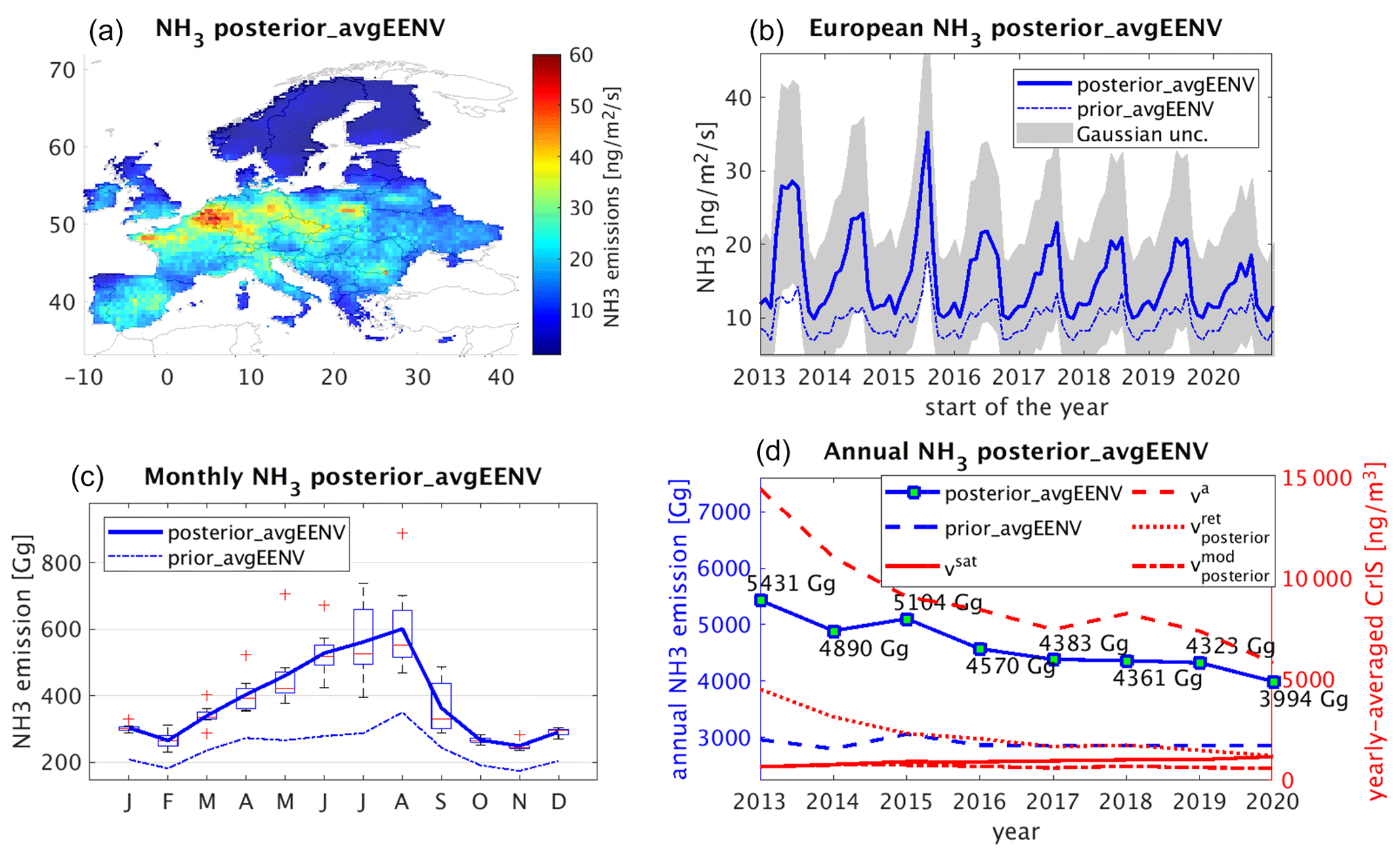
Figure 2The spatial distribution of posterior ammonia emissions (posterior_EENV, a) together with their temporal distributions (b). The Gaussian uncertainty of the posterior emissions is also plotted. Monthly average ammonia emissions are shown in the graph in (c). The monthly average posterior emissions over the studied period are accompanied by the boxplot where the red line indicates the median; the bottom and top edges of the boxes indicating the 25th and 75th percentiles, respectively; and the whiskers extend to the most extreme data points not considered to be outliers, which are denoted using red crosses. Solid blue lines refer to the posterior ammonia emissions, while dashed ones refer to the prior emissions (avgEENV). Finally, annual average ammonia emissions are also plotted (d). Except for the annual average emission dosages that are shown in blue, we also depict the elements that were used to calculate , namely va and (see Eq. 1), which were compared with vsat.
Figure 2b shows the annual posterior emissions discretized monthly for the whole period (solid line) compared to prior ammonia emissions (dashed line), averaged for the domain. Higher emissions than the prior ones were calculated, which is not necessarily attributed to emission increases over Europe but rather to miscalculation of emissions in the prior bottom-up inventories that were used. A strong seasonal cycle is also observed, peaking in the middle of each year (summer) of the study period, but for several of these years, the characteristic bimodal cycle also appears with another peak in spring (Beaudor et al., 2023).
To examine more closely the seasonal variability of ammonia emissions in Europe, we present the monthly posterior emissions of ammonia averaged for the whole study period (2013–2020) together with the prior ones in panel (c) of Fig. 2. The total emissions for each month based on the map element size and length of the respective month were averaged for the whole study period. The same was done for each year in panel (d). The interannual variability over the period between 2013 and 2020 is also apparent in the monthly boxplots and whisker plots of the posterior emissions. In addition, the spatial distribution of monthly ammonia emissions averaged for the 8-year period is given in Fig. S2. It appears that ammonia emissions are very low in wintertime (DJF average: 286 Gg) over Europe and increase towards summer (JJA average: 563 Gg) due to temperature-dependent volatilization of ammonia (Sutton et al., 2013), with the largest emissions occurring in August (601 Gg). Although a clear peak of fertilization in early spring is missing from the plot, emissions start to increase in early spring and peak in late summer (Van Damme et al., 2022), corresponding to the start and end of the fertilization periods in Europe (Paulot et al., 2014). Fertilization is tightly regulated in Europe (Ge et al., 2020). It is only allowed from February to mid-September in the Netherlands, while manure application is also only allowed during the same period, depending on the type of manure and the type of land (Van Damme et al., 2022). In Belgium, nitrogen fertilizers are only allowed from mid-February to the end of August (Van Damme et al., 2022), as is the case in Germany (restricted in winter months) (Kuhn, 2017).
Finally, Fig. 2 (bottom right) shows the annual posterior emissions for the whole period with the annual total emissions for each year. We observe a significant decrease in ammonia posterior emissions over Europe during the 2013–2020 period. Emissions were estimated to be 5431 Gg for 2013, decreasing to 4890 Gg in 2014. A minor increase can be seen in 2015 (5104 Gg), after which a significant decrease of 534 Gg (more than 10 %) was estimated, followed by the nearly constant plateau at the levels between 4383 Gg in 2017, 4323 Gg in 2019, and finally 3994 Gg in 2020. The gradual decrease in ammonia emissions over Europe since 2013 is also plotted spatially in Fig. S3. It is evident that the restrictions and measures adopted by the European Union to reduce secondary PM formation were successful as emissions in the hotspot regions of Belgium, the Netherlands, Germany, and Poland declined drastically over time. However, an increase of +4.4 % was observed in 2015. It has been reported that ammonia emissions increased in 2015, and several European Union member states, as well as the EU as a whole, exceeded their respective ammonia emission ceilings (EEA, 2017). The increase was reported to be +1.8 % and was mainly caused by increased emissions in Germany, Spain, France, and the United Kingdom. This was caused by extensive use of inorganic nitrogen fertilizers (including urea application) in Germany, while increased emissions in Spain were driven by an increase in the consumption of synthetic nitrogen fertilizers and in the number of cattle and pigs (EEA, 2017). It should be mentioned that a false decrease of ammonia in 2020 due to the COVID-19 pandemic is calculated by the current methodology, mainly due to bias created by the decreases in NOx and SO2, which are precursor species of the atmospheric acids with which ammonia reacts (see Tichý et al., 2022).
3.2 Country-by-country ammonia emissions
Posterior annual emissions of ammonia for 2013–2020 are plotted for four European regions (western, central and eastern, northern, and southern Europe), accompanied by relative trends calculated as the difference between the years 2013 and 2020 divided by the average for the whole period in the left panel of Fig. 3, while the estimated seasonal variation of each region is shown in the right panels, averaged over the whole 8-year period. Western Europe includes Ireland, Austria, France, Germany, Belgium, Andorra, Luxembourg, the Netherlands, Switzerland, and the United Kingdom; central and eastern Europe include Albania, Bosnia and Herzegovina, Bulgaria, Czechia, Croatia, Hungary, Belarus, Slovakia, North Macedonia, Montenegro, Poland, Romania, Moldova, Slovenia, Ukraine, and Serbia; northern Europe is defined by Denmark, Estonia, Finland, Latvia, Lithuania, the Faroe Islands, Norway, and Sweden; finally, southern Europe includes Cyprus, Greece, Italy, Portugal, and Spain.
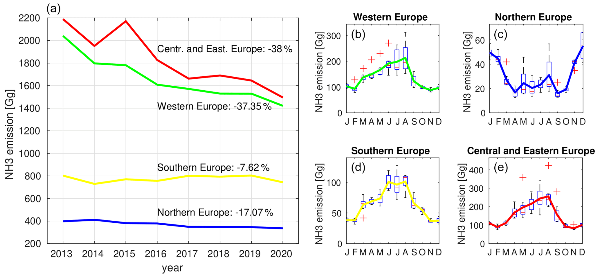
Figure 3(a) Annual posterior emissions of ammonia in southern (yellow), western (green), northern (blue), and central and eastern (red) Europe. (b–e) Monthly average posterior emissions of ammonia accompanied by boxplots, where the red line indicates the median; the bottom and top edges of the box indicate the 25th and 75th percentiles, respectively; and the whiskers extend to the most extreme data points (not considered to be outliers), which are represented using red crosses.
The most significant decreases in ammonia emissions were estimated to be −38 % in central and eastern Europe and −37 % in western Europe, respectively. Quantitatively, central and eastern Europe's emissions were estimated to gradually drop from 2190 Gg in 2013 to 1495 Gg in 2020, with a small increase in 2015 (2171 Gg), mainly because Germany, France, and the United Kingdom missed their emission targets (EEA, 2017). Western European emissions of ammonia also declined constantly over time from 2041 Gg in 2013 to 1421 Gg in 2020. Smaller, yet significant, decreases were calculated over northern Europe, from 398 Gg in 2013 to 333 Gg in 2020 (−17 %). Finally, southern Europe exhibited a minor drop between the years 2013 and 2014 (from 803 Gg in 2013 to 729 Gg in 2014), followed by a small increase until 2019 (from 729 to 803 Gg) and then a decrease again in 2020 to 743 Gg. Overall, southern European emissions decreased by −7.62 %.
The seasonal cycle of ammonia was again characterized by the restrictions applied to the agricultural-related activities by the European Union member states (Fig. 3b–e). As such, emissions in western, central and eastern, and southern Europe were very low in winter and started increasing when fertilization was allowed in early spring, whereas the increasing temperature towards summer increased volatilization and, thus, emissions of ammonia (Van Damme et al., 2022; Ge et al., 2020). Although much less marked than in other European regions due to lower prevailing temperatures and weaker agricultural applications, emissions in northern Europe show the spring–summer temperature dependence. However, emissions were estimated to be double in winter, rather following the cycle of SO2 (Tang et al., 2021). Emission may increase in northern Europe in winter because OH and O3 concentrations are much lower, and the rate of converting SO2 to sulfate is much slower. This means that less sulfate is produced, and thus, more NH3 stays in the gas form. Fig. S4 shows prior emissions in western, central and eastern, northern, and southern Europe for EC6G4 and NE emission inventories. Both show the aforementioned increase in emissions during winter in northeastern Europe. Specifically, the NE emissions that dominate the a priori emissions (avgEENV) as the highest inventory show an extreme winter peak in the north (emissions decline from 105 to 13 Gg). Therefore, there is a very strong dependence of the posterior seasonality of ammonia in northern Europe, which may also be influenced by the used prior emissions – see the uncertainty analysis in Sect. 3.3.
Country-specific emissions of posterior ammonia on a monthly basis (8-year average emissions) are shown for 20 countries in Fig. S5. For countries such as Portugal, Spain, Italy, the United Kingdom, the Netherlands, Belgium, Poland, Hungary, Denmark, Belarus, and Romania, two peaks can be clearly seen in late spring and at the end of summer. As discussed before, these peaks coincide with the two main fertilization periods in Europe (Paulot et al., 2014). However, it is expected that ammonia abundance is high throughout the entire spring–summer period (e.g. Greece, France, Germany, Czechia, Ukraine, and Bulgaria) due to agricultural activity and temperature-dependent volatilization (Sutton et al., 2013). Ammonia emissions in Finland, Sweden, and Norway are smaller than in the rest of Europe and show a reverse seasonality.
3.3 Uncertainties in ammonia's posterior emissions
For the calculation of the uncertainty of the estimated posterior emissions, two different approaches were used. The first approach is based on uncertainty arising as a result of the inversion methodology. The standard deviation is calculated from the posterior estimate, which is in the form of a Gaussian distribution such as
where N denotes the normal (Gaussian) distribution, and the posterior parameters μi and σi are the results of inversion for each element of the spatiotemporal domain. The uncertainty associated with any given spatial element is then a property of the Gaussian distribution defined with the square root of summed squared standard deviations:
Here, denotes the estimated variance of the emissions for given coordinates and a given time period; we consider the uncertainty calculated to be 2σ standard deviations; i.e. 95 % of the values lay inside the interval, with the centre in the reported emissions being surrounded by the reported uncertainty.
The second approach is based on the ensemble of the used prior emissions as an input for the inversion. The different ensemble members are built from five prior emissions (see Fig. 1), while the uncertainty is calculated as the standard deviation of five resulting posterior emissions.
The calculated posterior uncertainty for our spatial domain and studied period (2013–2020) is shown in Fig. 4 for the Gaussian posterior (left) and for the ensemble of prior emissions (right). The uncertainties associated with the Gaussian posterior for each year of the study period are depicted in Fig. S6. The absolute uncertainty of the Gaussian posterior ammonia emissions reaches a maximum of 23.3 ng m−2 s−1 or about 39 % (relative value, calculated based on the related maximum of posterior emissions). The uncertainty based on the prior ensemble reaches a maximum of 60.2 ng m−2 s−1, which is equal to about 101 % based on the related maximum of posterior emissions. In general, the patterns of both posterior uncertainties, the Gaussian posterior and the prior ensemble, are in agreement in terms of their patterns and follow the one of the posterior emissions, with the highest values over (i) Belgium, the Netherlands, and Germany due to livestock, farming, and agricultural activity; (ii) Poland, southern Romania, and Croatia due to industrial applications; (iii) Catalonia due to pig farming; and (iv) western France due to manure application. Nevertheless, the obtained posterior uncertainty remains low, and this depicts the robustness of the methodology used and the calculated posterior emissions of ammonia.
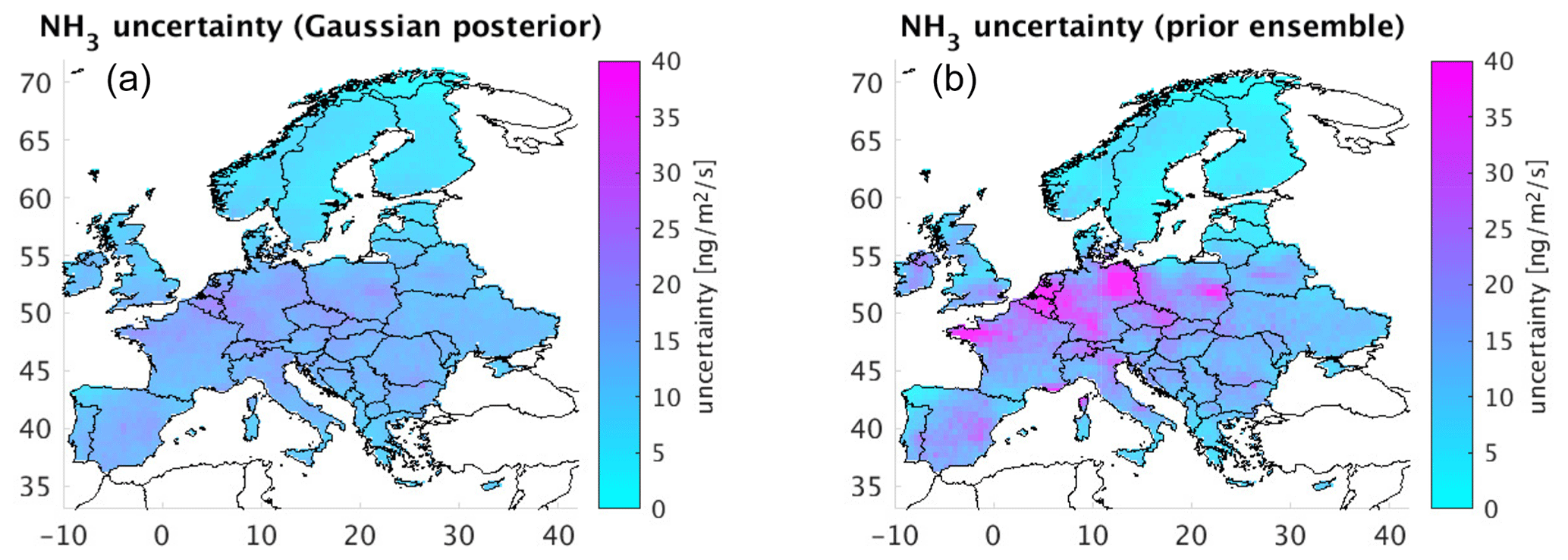
Figure 4Absolute uncertainty of posterior emissions of ammonia calculated as 2σ (a) and from a member ensemble (b) comprising posterior emissions calculated with five different priors (Fig. 1) averaged for the whole study period of 2013–2020.
3.4 Validation of posterior emissions
As shown in Eq. (3) (Sect. 2.4), the inversion algorithm minimizes the difference between the satellite observations (vsat) and the retrieved ammonia concentrations (vret). The latter is a function of different satellite parameters (e.g. averaging kernel sensitivities) and modelled ammonia concentrations using a prior dataset (vmod or vtrue), as seen in Eq. 1. The overall result is always propagated to vmod iteratively, each time updating the prior emissions to obtain posterior ammonia. As specified in CrIS guidelines, modelled concentrations (vmod) cannot be directly compared with satellite data (vsat), while comparing vsat with vret is not a proper validation method because the comparison is performed for satellite observations that were included in the inversion (dependent observations), and the inversion algorithm has been designed to reduce the vsat–vret mismatches. This means that the reduction of the posterior retrieved concentration's (vret) mismatch to the observations (vsat) is determined by the weighting that is given to the observations with respect to vret. A proper validation of the posterior emissions is performed against observations that were not included in the inversion (independent observations).
For these reasons, we compare modelled posterior concentrations of ammonia (vmod) at the surface with ground-based observations over Europe from the EMEP (European Monitoring and Evaluation Programme, https://emep.int/mscw/, last access: 26 October 2023) network (Torseth et al., 2012). The measurements are open to the public and can be retrieved from https://ebas.nilu.no, last access: 26 October 2023. We used measurements for all the years between 2013 and 2020 from an average of 53 stations, with 2928 observations for each station covering all Europe (Fig. S7). The comparison is plotted for each of the 53 stations separately on a Taylor diagram in Fig. 5. For all stations, the Pearson's correlation coefficient increased, for the posterior ammonia (coloured circles) increased as compared to the prior one (coloured squares), reaching above 0.6 at several stations, while the normalized root mean square error (nRMSE) and standard deviation were kept below 2 (unitless) and 2 µg m−3, respectively, at almost all stations (except SI0008 in Slovenia).
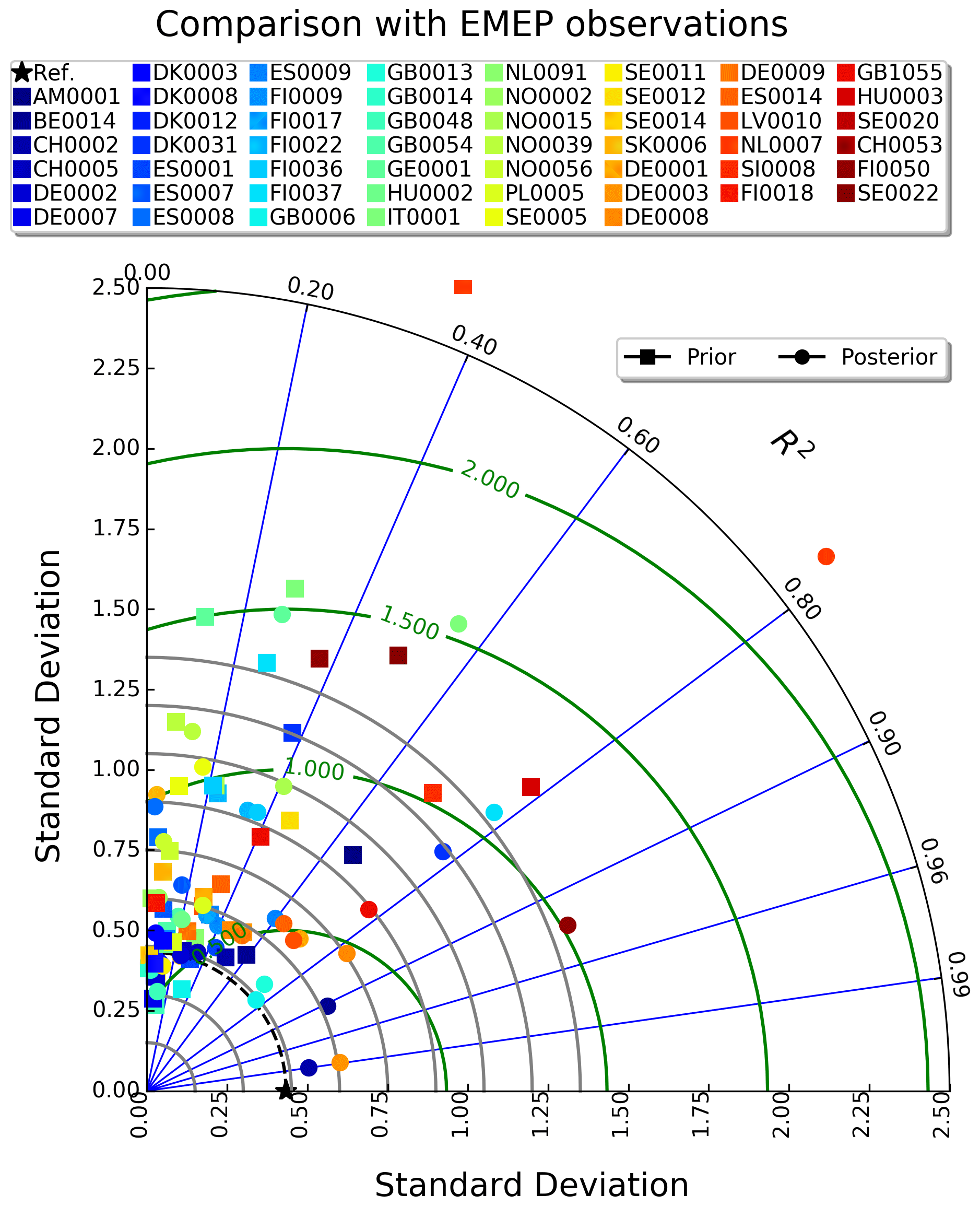
Figure 5Modelled concentrations of ammonia with prior and posterior emissions against ground-based observations from 53 EMEP stations for 2013–2020 presented in a Taylor diagram. The diagram shows the Pearson's correlation coefficient (gauging similarity in terms of pattern between the modelled and observed concentrations) that is related to the azimuthal angle (blue contours); the standard deviation of modelled concentrations of ammonia is proportional to the radial distance from the origin (black contours), and the centred normalized RMSE of modelled concentrations is proportional to the distance from the reference standard deviation (green contours).
To further show how posterior emissions of ammonia affect modelled concentrations, we chose six stations (DE0002 in Germany, NO0056 in southern Norway, ES0009 in Spain, NL0091 in the Netherlands, HU0002 in Hungary, and PL0005 in Poland) from the EMEP network (highlighted in red in Fig. S7), and we plot prior and posterior concentrations against ground-based ammonia over time for the whole study period (2013–2020) in Fig. S8. Given the long period of plotting, we average observations every week and modelled concentrations every month for a more visible representation of the comparison. To evaluate the comparison, we calculate a number of statistic measures, namely nRMSE, the normalized mean absolute error (nMAE), and the root mean squared logarithmic error (RMSLE), as defined below:
where n is sample size, and m and o are the individual sample points for model concentrations and observations of ammonia indexed with i. As one can see in Fig. S8, all statistics were improved in all six stations, and posterior concentrations were closer to the observations. However, individual peaks were, in many cases, misrepresented in the model. Whether this is a result of the measurement technique or the fact that local sources cannot be resolved at the spatiotemporal resolution of CTM and FLEXPART (given the short lifetime of atmospheric ammonia) needs further research. The best results were obtained at station ES0009 (Spain), where the model captured the seasonal variation of the observations during the whole study period (2013–2020). In all other stations, the seasonality is maintained, albeit steep peaks in the observations are lost.
As explained in Sect. 1, ammonia reacts with the available atmospheric acids, producing secondary aerosols (Seinfeld and Pandis, 2000). Therefore, its presence and lifetime in the atmosphere is driven by the atmospheric acids and their precursors, SO2 and NO2. Changes in the atmospheric levels of these substances have a significant impact on the lifetime of ammonia and its emissions, as highlighted in Tichý et al. (2022). Therefore, it is clear that a wrong representation of the trends in modelled SO2 and NO2 will lead to systematic biases in the estimated ammonia emission trends. To further demonstrate that the modelling system correctly represents the trends in SO2 and NO2, we compare ground-based observations of these two species from the EMEP network (https://emep.int/mscw/, last access: 26 October 2023) against modelled concentrations.
The comparison is shown in Fig. S9 for six random EMEP stations for different years for NO2 and SO2. The full comparison of the two datasets of observations is plotted in scatterplots of modelled versus measured surface concentrations for NO2 and SO2 for the whole of the study period (2013–2020) in Fig. S10. Total numbers of 3 368 660 for SO2 and 4 252 592 for NO2 were used in the validation. It is evident that the seasonal variations of the modelled surface concentrations and their magnitudes are both represented very well in the model for NO2 and SO2. nRMSE was 0.12–0.19 for NO2 and 0.09–0.25 for SO2, nMAE was 0.39–0.94 for NO2 and 0.48–1.2 for SO2, and RMSLE was 0.25–0.49 for NO2 and 0.11–0.33 for SO2 in the six stations (Fig. S9). For over 4.2 and 3.3 million measurements in this validation of NO2 and SO2 concentrations for 2013–2020 study period, nRMSE values were 0.05 and 0.02, nMAE values were 0.74 and 1.0, and RMSLE values were 0.50 and 0.40 for NO2 and SO2, respectively (Fig. S10).
4.1 Comparison with emissions inferred from satellite observations
We compared our posterior estimates with two recently published studies on ammonia emissions in Europe (Cao et al., 2022; Luo et al., 2022). Luo et al. (2022) used IASI observations for the period 2008–2018 to estimate ammonia emissions in a global domain. Their method was based on updating prior emissions with correction terms computed using differences between observed and simulated ammonia columns combined with calculated ammonia lifetimes. The key indicators calculated for the European domain in Luo et al. (2022) are a linear trend for the 2008–2018 period, average annual emissions, and relative trends. Note that we compare our 8-year period with the decade in Luo et al. (2022). The comparison is depicted in Fig. 6. Our estimates (Fig. 6a) are in good agreement with those calculated by Luo et al. (2022). The linear trend was estimated as −1.27 Tg for the period by Luo et al. (2022), while our estimate is −1.44 Tg. The spatial distribution of the trend is also given in Fig. 6a. The key decrease is observed mainly in France, Germany, and middle Europe, while the increasing trend is observed mostly in Spain, parts of Italy, and Greece. The average annual ammonia emission for the European domain in Luo et al. (2022) was estimated to be 5.05 Tg, while our estimate is 4.63 Tg. Our lower estimate (by approximately 8 %) might be attributed to the use of a more recent period in our study, but both methods agree that the trend in Europe is negative. The relative decrease estimated by Luo et al. (2022) is −25.1 %, while we calculate −31.02 %, which is again in very good agreement.
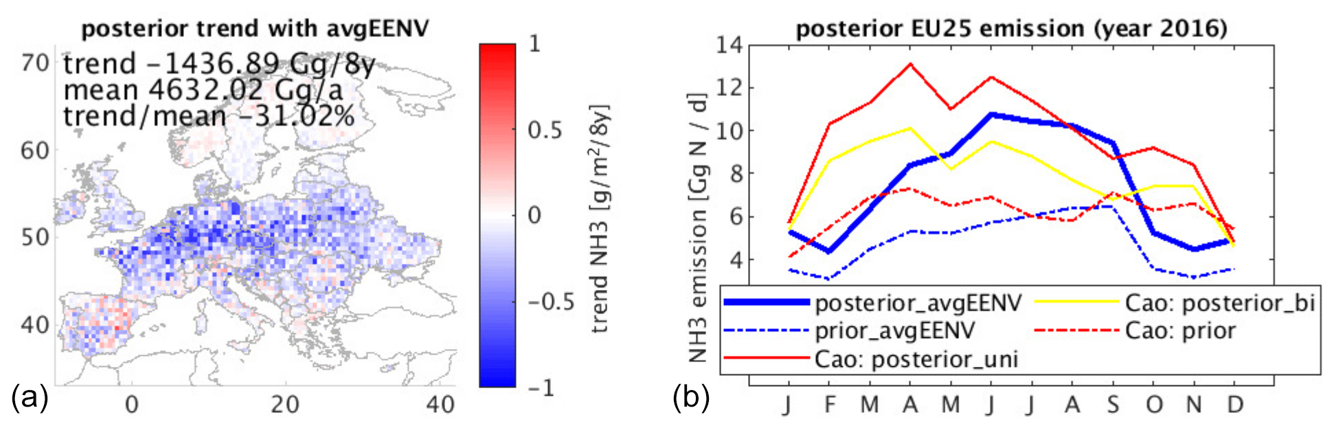
Figure 6(a) Spatial distribution of ammonia emission trends computed for the studied period 2013–2020 in the same way as in Luo et al. (2022), where trend, mean, and trend–mean are defined or computed in the same way. (b) Comparison of ammonia emissions from the EU25 countries for the year 2016 from our posterior calculations (posterior_avgEENV in blue) and results from Cao et al. (2022) (posterior_uni in red and posterior_bi in yellow).
Cao et al. (2022) used CrIS observations for the year 2016 in order to estimate ammonia emissions for 25 European Union members (EU25), namely Austria, Belgium, Bulgaria, Croatia, Republic of Cyprus, Czech Republic, Denmark, Estonia, France, Germany, Greece, Hungary, Ireland, Italy, Latvia, Lithuania, Luxembourg, Malta, Netherlands, Poland, Portugal, Romania, Slovakia, Slovenia, and Spain. The method was tested with uni-directional and bi-directional flux schemes. The uni-directional dry-deposition scheme assumes only an air-to-surface exchange of ammonia, ignoring changes in environmental conditions, while the bi-directional scheme captures dynamics in measured ammonia fluxes. Total estimated ammonia emissions for the EU25 region from the uni-directional scheme (posterior_uni) and the bi-directional scheme (posterior_bi) were reported to be 3534 and 2850 Gg N yr−1, respectively. The posterior_bi estimate is very close to our estimate for EU25 for the year 2016, which is 2712 Gg N yr−1, while the posterior_uni is approximately 30 % higher. A uni-directional dry-deposition scheme ignores the impacts of changes in environmental conditions (e.g. soil temperature, soil wetness, soil pH, fertilized condition, and vegetation type) on ammonia emissions from fertilized soil and crops (volatilization), which likely leads to high biases in top-down estimates. Ammonia in the LMDz-OR-INCA model, which was used to capture ammonia's losses, resembles a partially bi-directional treatment, where emissions and deposition are both possible at the same time without any use of a compensation point; this may explain this 30 % difference.
The detailed EU25 emissions for the year 2016 are displayed in Fig. 6 (right panel) for posterior_uni (red), posterior_bi (yellow), our post_avgEENV (blue), and priors used by Cao et al. (2022) and in our study (dashed red and blue, respectively). As seen from Fig. 6, our posterior estimates (post_avgEENV) have more similar characteristics in relation posterior_bi, with the monthly difference being less than a factor of 2 positive or negative compared to Cao et al. (2022). Note that the posterior_uni estimates are always a factor of 3 higher than our posterior estimates for ammonia emissions. The main differences can be observed during the February–March and October–November periods, where our estimates are generally lower than those from Cao et al. (2022). Finally, Cao et al. (2022) reported more of a springtime peak that is likely associated with crop fertilization, whereas in this study, the peak is towards the warmer season (volatilization) due to livestock sources.
4.2 Assessment of ammonia's atmospheric linearities
Ammonia is a particularly interesting substance due to its affinity for reacting with atmospheric acids that produce secondary aerosols. In most cases, it is depleted by sulfuric and nitric acids. However, when relative humidity is high and when particles are aqueous, sulfate reacts with ammonia and decreases, while the equilibrium vapour pressure of ammonia with nitric acid increases, shifting the reaction towards the production of free ammonia (Seinfeld and Pandis, 2000). The former reaction is a rare event, and lots of prerequisites must be fulfilled to take place.
Fig. S11a shows the frequency distribution of gain (production of free ammonia – negative numbers) or loss (production of sulfate or nitrate – positive numbers) due to all chemical processes in the inversion domain (25–75∘ N, 10∘ W–50∘ E) for the study period (2013–2020) and for the lowest six sigma-p vertical levels (∼ 1018–619 hPa; see averaging kernels in Sect. 2.1) (Sitwell et al., 2022). The figure shows mostly positive numbers, indicating that atmospheric ammonia reacts towards secondary aerosol formation. The spatial distribution of the gain or loss of ammonia is shown in Fig. S11b. The pixels indicating the production of gaseous ammonia are located in marine regions, where we chose to not perform inversions as these are 1 order of magnitude lower (Bouwman et al., 1997) and are thus less significant. No continental pixels showing a gain of ammonia were detected, which would cause simulations made backwards in time to fail with our Lagrangian model (see next paragraph). Our approximation, although simplistic, provides computational efficiency when simulating SRMs in backward mode using FLEXPART (Pisso et al., 2019).
Seibert and Frank (2004) reported that standard Lagrangian particle dispersion models cannot simulate non-linear chemical reactions. First-order chemical reactions, where the reaction rates can be prescribed, are also linear. Non-linear chemistry cannot be calculated because the background chemistry nor the coupling of the tracked plume (forwards or backwards) to this background are modelled. Technically, the SRM in FLEXPART is calculated for a receptor with a certain mean mixing ratio (χ) and an emitting source (qi,n) in a certain discretization of the space (index i) and time (index n):
where J is the total number of backward trajectories (particle index j) originating from the position of the receptor χ and ending at a certain discretized time (index n) in a certain discretized space position (index i) for a time interval , and where the air density is ρi,n. The further function pj,n () represents the relative (in relation to the initial receptor state) decay of the mass value in the particle in its travel from the receptor to the discretized space time interval (jn) due to any linear decay process (e.g. deposition, linear chemical decay) for a perfectly conserved scalar . So, for linearly decaying species, a direct SRM can be calculated explicitly among all relevant receptor points and all positions in space and time. The existence of the SRM (H), linking directly mixing ratios at the receptor points with emissions, is the prerequisite to apply simple inversion algorithms, such as the one in the present study.
The inversion of observations to obtain emissions for non-linear chemically reactive species entails the need for a chemistry transport model (CTM) forwards (and, its adjoint, backwards) in time – from time t0 to time t – that evolves the full state of the atmosphere in relation to the emissions and boundary conditions. Subsequently, a cost function is evaluated by an iterative descent gradient method that implies running the adjoint of the forward model (Fortems-Cheiney et al., 2021). Note that an iterative algorithm means that the forward and adjoint models run several times in sequence until the estimated minimum of the cost function is reached.
To overcome these complexities, we examine the linearities of our method and show that FLEXPART simulates ammonia efficiently, and we evaluate modelled ammonia against ground-based measurements of ammonia from EMEP (https://emep.int/mscw/, last access: 26 October 2023) in Europe, EANET (East Asia acid deposition NETwork) in southeastern Asia (https://www.eanet.asia/, last access: 26 October 2023), and AMoN (Ammonia Monitoring Network in the US, AMoN-US; National Air Pollution Surveillance Program (NAPS) sites in Canada) in North America (http://nadp.slh.wisc.edu/data/AMoN/, last access: 26 October 2023). The SRMs for ammonia express the emission sensitivity (in seconds) and yield modelled concentrations at the receptor point when coupled with gridded emissions from EGG (in kg m−2 s−1; see Sect. 2.2) at the lowest model level (100 m). To check the consistency of the proxy used in the SRMs of ammonia, we also simulated surface concentrations of ammonia with FLEXPART in forward mode using the same emissions (EGG). We have chosen two random ground-based stations from each of the three measuring networks (EMEP, EANET, AMoN) to compare modelled concentrations. For consistency, we also plot the resulting surface concentrations from the LMDz-OR-INCA model (Fig. S12).
Modelled concentrations (forward and backward FLEXPART and the CTM LMDz-OR-INCA) at each station have been averaged to the temporal resolution of the observations. Fig. S13 shows Taylor diagrams of the comparison between FLEXPART simulated concentrations in forward and backward mode. Plotting backward versus forward results is a common procedure to infer whether a Lagrangian model produces reasonable results (Eckhardt et al., 2017; Pisso et al., 2019). In general, the forward and backward simulations show very good agreement for the depicted receptor points. For example, ammonia concentrations at stations AL99, CA83, and VNA001 (Fig. S12) are simulated similarly, and the mean concentrations are almost identical in the forward and backward modes. However, during some episodes, there can be notable differences (e.g. at DE0002R), as seen before (Eckhardt et al., 2017). The main reason is that the backward calculations always give more accurate results as the number of particles released at the receptor is much higher in backward mode than in forward mode; the particles are targeted towards a very small location in backward mode, whereas in forward mode, the particles are distributed equally on a global scale, and therefore, fewer particles represent each receptor location. Another reason is that transport and, especially, turbulent processes are parameterized by random motions, which are different for each FLEXPART simulation. Finally, the coordinate system for defining the height layer above the ground depends on the meteorological field which is read at the start of the simulation, and this can also cause small deviations. The Taylor diagram for the respective comparison (Fig. S13) shows high Pearson's correlation coefficients (>0.7), low standard deviations (<1 µg N m−3), and low root mean square errors (RMSEs <0.7 µg N m−3).
4.3 Limitations of the present study
The latest Commission Third Clean Air Outlook published in December 2022 (EC, 2022), which is based on data reported by the EEA (https://www.eea.europa.eu/data-and-maps/dashboards/necd-directive-data-viewer-7, last access: 26 October 2023), concluded (p. 2) that emissions of ammonia in recent years remain worryingly flat or may have increased for some member states. The assessment covers the period we investigated in the present paper (2013–2020) and shows (for the EU27) a reduction in ammonia emissions of only 2 %, which is far smaller than that which we calculated here (26 %). The consistency of our results with those calculated with similar methodologies (Cao et al., 2022; Luo et al., 2022) urges us to believe that such differences in ammonia trends are the result of differences between bottom-up and top-down methodologies.
Another reason for the difference in emissions between EC (2022) and this study might be the fact that we used both nighttime and daytime CrIS observations. The nighttime observations use the exact same retrieval approach as the daytime ones. Any unknown bias would only be present if atmospheric conditions are such that they make the retrievals more challenging during night overpasses (e.g. thermal inversions causing a radiative emission layer at the surface). Note that CrIS nighttime observations have not been validated yet.
CrIS ammonia retrievals are performed in the logarithmic space and are expressed by Eq. (1). When solving the cost function in the inverse-modelling algorithm, we minimize the model–observation mismatch, which, in the present case, is vret (calculated using modelled concentrations, vtrue=vmod, in Eq. (1) after applying prior emissions) with the CrIS observations, vsat. Then, iteratively, the algorithm updates vmod to calculate the posterior emissions using Eq. (1). The logarithmic nature of Eq. (1) causes (i) the optimization of the modelled concentrations (vmod) to be tiny and (ii) the trend of the posterior emissions to have a very large dependency on the prior column used in CrIS (va). The latter is shown very clearly in Fig. 2d.
Today, there is a large debate about ammonia abatement strategies for Europe but also for southeastern Asia in an effort to reduce secondary formation and, thus, to mitigate climate crises (van Vuuren et al., 2015). These strategies include (a) low-nitrogen feed by reducing ammonia emissions at many stages of manure management, from excretion in housing, through storage of manure, to the application on land, which would also have positive effects on animal health and indoor climate (Montalvo et al., 2015); (b) low-emission livestock housing, which focuses on reducing the surface area on which and the time over which manure is exposed to air by adopting rules and regulations regarding new livestock houses (Poteko et al., 2019); and (c) air purification by adopting technologies to clean exhaust air from livestock buildings (Cao et al., 2023), amongst others. Here we used satellite observations from CrIS and a novel inverse-modelling algorithm to study the spatial variability and seasonality of ammonia emissions over Europe. We then evaluated the overall impact of such strategies on the emissions of ammonia for the period 2013–2020. The main key messages can be summarized below:
-
The highest emissions over the 2013–2020 study period occur in northern Europe (Belgium, the Netherlands, and northwestern Germany). At a regional scale, peaks are seen in western Europe (Poland, southern Romania, and Croatia) due to industrial activities, in Spain (Ebro Valley, Aragon, and Catalonia) due to agricultural activities and farming, and in Belgium and the Netherlands due to livestock activity (dairy cow, beef cattle, pig, and chicken farming).
-
Ammonia emissions are low in winter (average: 286 Gg) and peak in summer (average: 563 Gg) due to temperature-dependent volatilization of ammonia, while a notable peak attributed to fertilization can be seen in early spring during some years.
-
Over the 2013–2020 period, European emissions of ammonia decreased from 5431 Gg in 2013 to 3994 Gg in 2020 (about −26 %). Hence, the restrictions adopted by the European Union members were effective in reducing secondary PM formation.
-
A slight emission increase of +4.4 % in 2015 appears for several European Union member states (Germany, Spain, France, and the United Kingdom) who exceeded their respective ammonia emission targets. Part of the 2020 ammonia decrease might be attributable to the COVID-19 pandemic restrictions.
-
The largest decreases in ammonia emissions were observed in central and eastern Europe (−38 %, 2190 Gg in 2013 to 1495 Gg in 2020) and in western Europe (−37 %, 2041 Gg in 2013 to 1421 Gg in 2020). Smaller decreases were calculated in northern Europe (−17 %, 398 Gg in 2013 to 333 Gg in 2020) and southern Europe (−7.6 %, from 803 Gg in 2013 to 743 Gg in 2020).
-
The maximum calculated absolute uncertainty of the Gaussian posterior model was 23.3 ng m−2 s−1 or about 39 % (relative value), and the calculated maximum of prior emissions was 60.2 ng m−2 s−1 or about 101 % following the spatial distribution of the posterior emissions.
-
Comparison of the concentrations calculated with prior and posterior ammonia emissions against independent (not used in the inversion algorithm) observations showed improved correlation coefficients and low nRMSEs and standard deviations. Looking at the time series of six randomly selected stations in Europe, we also found that posterior surface concentrations of ammonia were in accordance with the ground-based measurements, also following the observed seasonal trends.
-
Our results agree very well with those from Luo et al. (2022) (decreasing trend: −1.44 versus −1.27 Tg, annual European emissions: 4.63 versus 5.05 Tg) and those from Cao et al. (2022) following their methodology (their posterior_bi estimate for EU25 for the year 2016 was 2850 Gg N yr−1, while we calculate 2712 Gg N yr−1).
-
The relatively low posterior uncertainty and improved statistics in the validation of the posterior surface concentrations denote the robustness of the posterior emissions of ammonia calculated with satellite measurements and our adapted inverse framework.
The data generated for the present paper can be downloaded from Zenodo (https://doi.org/10.5281/zenodo.7646462, Tichý et al., 2023). FLEXPARTv10.4 is open access and can be downloaded from Pisso et al. (2019), while the use of ERA5 data is free of charge, worldwide, non-exclusive, royalty free, and perpetual. The inversion algorithm LS-APC is open access from https://www.utia.cas.cz/linear_inversion_methods (Tichý, 2023). CrIS ammonia can be obtained by request to Mark Shephard (mark.shephard@ec.gc.ca). EMEP measurements are open to the public at https://ebas.nilu.no (EBAS, 2023). FLEXPART SRMs for 2013–2020 can be obtained from the corresponding author upon request.
The supplement related to this article is available online at: https://doi.org/10.5194/acp-23-15235-2023-supplement.
OT adapted the inversion algorithm, performed the calculations and analyses and wrote the paper. SE adapted FLEXPARTv10.4 to model ammonia chemical loss. YB and DH set up the CTM model and performed the simulation, the output of which was used as input in FLEXPART. NE performed the FLEXPART simulations, contributed to analyses, and wrote and coordinated the paper. All the authors contributed to the final version of the paper.
At least one of the (co-)authors is a member of the editorial board of Atmospheric Chemistry and Physics. The peer-review process was guided by an independent editor, and the authors also have no other competing interests to declare.
Publisher's note: Copernicus Publications remains neutral with regard to jurisdictional claims made in the text, published maps, institutional affiliations, or any other geographical representation in this paper. While Copernicus Publications makes every effort to include appropriate place names, the final responsibility lies with the authors.
This study was supported by the Research Council of Norway (project ID no. 275407, COMBAT – Quantification of Global Ammonia Sources constrained by a Bayesian Inversion Technique). We kindly acknowledge Mark Shephard for providing CrIS ammonia. This work was granted access to the HPC resources of TGCC under the allocation no. A0130102201 made by GENCI (Grand Equipement National de Calcul Intensif). Ondřej Tichý was supported by the Czech Science Foundation (grant no. GA20-27939S). Special thanks are given to Massimo Cassiani for explaining the Lagrangian modelling basics in Sect. 4.2.
This research has been supported by the Norges Forskningsråd (grant no. 275407).
This paper was edited by Leiming Zhang and reviewed by Karen Cady-Pereira and one anonymous referee.
Abbatt, J. P. D., Benz, S., Cziczo, D. J., Kanji, Z., Lohmann, U., and Mohler, O.: Solid Ammonium Sulfate Aerosols as Ice Nuclei: A Pathway for Cirrus Cloud Formation, Science, 313, 1770–1773, 2006.
Beaudor, M., Vuichard, N., Lathière, J., Evangeliou, N., Van Damme, M., Clarisse, L., and Hauglustaine, D.: Global agricultural ammonia emissions simulated with the ORCHIDEE land surface model, Geosci. Model Dev., 16, 1053–1081, https://doi.org/10.5194/gmd-16-1053-2023, 2023.
Behera, S. N., Sharma, M., Aneja, V. P., and Balasubramanian, R.: Ammonia in the atmosphere: A review on emission sources, atmospheric chemistry and deposition on terrestrial bodies, Environ. Sci. Pollut. Res., 20, 8092–8131, https://doi.org/10.1007/s11356-013-2051-9, 2013.
Bouwman, A. F., Lee, D. S., Asman, W. A. H., Dentener, F. J., Van Der Hoek, K. W., and Olivier, J. G. J.: A global high-resolution emission inventory for ammonia, Global Biogeochem. Cy., 11, 561–587, https://doi.org/10.1029/97GB02266, 1997.
Cao, H., Henze, D. K., Shephard, M. W., Dammers, E., Cady-Pereira, K., Alvarado, M., Lonsdale, C., Luo, G., Yu, F., Zhu, L., Danielson, C. G., and Edgerton, E. S.: Inverse modeling of NH3 sources using CrIS remote sensing measurements, Environ. Res. Lett., 15, 104082, https://doi.org/10.1088/1748-9326/abb5cc, 2020.
Cao, H., Henze, D. K., Zhu, L., Shephard, M. W., Cady-Pereira, K., Dammers, E., Sitwell, M., Heath, N., Lonsdale, C., Bash, J. O., Miyazaki, K., Flechard, C., Fauvel, Y., Kruit, R. W., Feigenspan, S., Brümmer, C., Schrader, F., Twigg, M. M., Leeson, S., Tang, Y. S., Stephens, A. C. M., Braban, C., Vincent, K., Meier, M., Seitler, E., Geels, C., Ellermann, T., Sanocka, A., and Capps, S. L.: 4D-Var Inversion of European NH3 Emissions Using CrIS NH3 Measurements and GEOS-Chem Adjoint With Bi-Directional and Uni-Directional Flux Schemes, J. Geophys. Res.-Atmos., 127, 1–25, https://doi.org/10.1029/2021JD035687, 2022.
Cao, T., Zheng, Y., Dong, H., Wang, S., Zhang, Y., and Cong, Q.: A new air cleaning technology to synergistically reduce odor and bioaerosol emissions from livestock houses, Agr. Ecosyst. Environ., 342, 108221, https://doi.org/10.1016/j.agee.2022.108221, 2023.
Cassiani, M., Stohl, A., and Brioude, J.: Lagrangian Stochastic Modelling of Dispersion in the Convective Boundary Layer with Skewed Turbulence Conditions and a Vertical Density Gradient: Formulation and Implementation in the FLEXPART Model, Bound.-Lay. Meteorol., 154, 367–390, https://doi.org/10.1007/s10546-014-9976-5, 2014.
Clarisse, L., Van Damme, M., Clerbaux, C., and Coheur, P. F.: Tracking down global NH3 point sources with wind-adjusted superresolution, Atmos. Meas. Tech., 12, 5457–5473, https://doi.org/10.5194/amt-12-5457-2019, 2019.
Crippa, M., Solazzo, E., Huang, G., Guizzardi, D., Koffi, E., Muntean, M., Schieberle, C., Friedrich, R., and Janssens-Maenhout, G.: High resolution temporal profiles in the Emissions Database for Global Atmospheric Research, Sci. Data, 7, 1–17, https://doi.org/10.1038/s41597-020-0462-2, 2020.
D'Errico, J.: Inpaint_nans [code], https://www.mathworks.com/matlabcentral/fileexchange/4551-inpaint_nans, last access: 26 October 2023.
Dammers, E., Palm, M., Van Damme, M., Vigouroux, C., Smale, D., Conway, S., Toon, G. C., Jones, N., Nussbaumer, E., Warneke, T., Petri, C., Clarisse, L., Clerbaux, C., Hermans, C., Lutsch, E., Strong, K., Hannigan, J. W., Nakajima, H., Morino, I., Herrera, B., Stremme, W., Grutter, M., Schaap, M., Kruit, R. J. W., Notholt, J., Coheur, P. F., and Erisman, J. W.: An evaluation of IASI-NH 3 with ground-based Fourier transform infrared spectroscopy measurements, Atmos. Chem. Phys., 16, 10351–10368, https://doi.org/10.5194/acp-16-10351-2016, 2016.
Dammers, E., Shephard, M. W., Palm, M., Cady-Pereira, K., Capps, S., Lutsch, E., Strong, K., Hannigan, J. W., Ortega, I., Toon, G. C., Stremme, W., Grutter, M., Jones, N., Smale, D., Siemons, J., Hrpcek, K., Tremblay, D., Schaap, M., Notholt, J., and Erisman, J. W.: Validation of the CrIS fast physical NH3 retrieval with ground-based FTIR, Atmos. Meas. Tech., 10, 2645–2667, https://doi.org/10.5194/amt-10-2645-2017, 2017.
Dammers, E., McLinden, C. A., Griffin, D., Shephard, M. W., Van Der Graaf, S., Lutsch, E., Schaap, M., Gainairu-Matz, Y., Fioletov, V., Van Damme, M., Whitburn, S., Clarisse, L., Cady-Pereira, K., Clerbaux, C., Francois Coheur, P., and Erisman, J. W.: NH3 emissions from large point sources derived from CrIS and IASI satellite observations, Atmos. Chem. Phys., 19, 12261–12293, https://doi.org/10.5194/acp-19-12261-2019, 2019.
Dee, D. P., Uppala, S. M., Simmons, A. J., Berrisford, P., Poli, P., Kobayashi, S., Andrae, U., Balmaseda, M. A., Balsamo, G., Bauer, P., Bechtold, P., Beljaars, A. C. M., van de Berg, L., Bidlot, J., Bormann, N., Delsol, C., Dragani, R., Fuentes, M., Geer, A. J., Haimberger, L., Healy, S. B., Hersbach, H., Hólm, E. V., Isaksen, L., Kållberg, P., Köhler, M., Matricardi, M., Mcnally, A. P., Monge-Sanz, B. M., Morcrette, J. J., Park, B. K., Peubey, C., de Rosnay, P., Tavolato, C., Thépaut, J. N., and Vitart, F.: The ERA-Interim reanalysis: Configuration and performance of the data assimilation system, Q. J. R. Meteorol. Soc., 137, 553–597, https://doi.org/10.1002/qj.828, 2011.
EBAS: Data from European Observatories, EBAS [data set], http://ebas.nilu.no/, last access: 26 October 2023.
EC: Report from the Commission to the European Parliament, the Council, the european Economic and Social Committee of the regions: The Third Clean Air Outlook, Brussels, European Commission, Directorate-General for Environment, 2022.
Eckhardt, S., Cassiani, M., Evangeliou, N., Sollum, E., Pisso, I., and Stohl, A.: Source-receptor matrix calculation for deposited mass with the Lagrangian particle dispersion model FLEXPART v10.2 in backward mode, Geosci. Model Dev., 10, 4605–4618, https://doi.org/10.5194/gmd-10-4605-2017, 2017.
EEA: European Union emission inventory report 1990–2015 under the UNECE Convention on Long-range Transboundary Air Pollution, https://www.eea.europa.eu/publications/annual-eu-emissions-inventory-report (last access: 26 October 2023), 2017.
Emanuel, K. A.: A Scheme for Representing Cumulus Convection in Large-Scale Models, J. Atmos. Sci., 48, 2313–2329, https://doi.org/10.1175/1520-0469(1991)048<2313:ASFRCC>2.0.CO;2, 1991.
Erisman, J. W., Bleeker, A., Galloway, J., and Sutton, M. S.: Reduced nitrogen in ecology and the environment, Environ. Pollut., 150, 140–149, https://doi.org/10.1016/j.envpol.2007.06.033, 2007.
Evangeliou, N., Balkanski, Y., Eckhardt, S., Cozic, A., Van Damme, M., Coheur, P.-F., Clarisse, L., Shephard, M., Cady-Pereira, K., and Hauglustaine, D.: 10–Year Satellite–Constrained Fluxes of Ammonia Improve Performance of Chemistry Transport Models, Atmos. Chem. Phys., 21, 4431–4451, https://doi.org/10.5194/acp-21-4431-2021, 2021.
Fang, S., Dong, X., Zhuang, S., Tian, Z., Zhao, Y., Liu, Y., Liu, Y., and Sheng, L.: Inversion of 137Cs emissions following the fukushima accident with adaptive release recovery for temporal absences of observations, Environ. Pollut., 317, 120814, https://doi.org/10.1016/j.envpol.2022.120814, 2023.
Forster, C., Stohl, A., and Seibert, P.: Parameterization of convective transport in a Lagrangian particle dispersion model and its evaluation, J. Appl. Meteorol. Climatol., 46, 403–422, https://doi.org/10.1175/JAM2470.1, 2007.
Fortems-Cheiney, A., Pison, I., Broquet, G., Dufour, G., Berchet, A., Potier, E., Coman, A., Siour, G., and Costantino, L.: Variational regional inverse modeling of reactive species emissions with PYVAR-CHIMERE-v2019, Geosci. Model Dev., 14, 2939–2957, https://doi.org/10.5194/gmd-14-2939-2021, 2021.
Fowler, D., Muller, J. B. A., Smith, R. I., Dragosits, U., Skiba, U., Sutton, M. A., and Brimblecombe, P.: A chronology of nitrogen deposition in the UK, Water Air Soil Pollut. Focus, 4, 9–23, 2004.
Galloway, J. N., Aber, J. D., Erisman, J. A. N. W., Seitzinger, S. P., Howarth, R. W., Cowling, E. B., and Cosby, B. J.: The Nitrogen Cascade, Bioscience, 53, 341–356, https://doi.org/10.1641/0006-3568(2003)053[0341:TNC]2.0.CO;2, 2003.
Ge, X., Schaap, M., Kranenburg, R., Segers, A., Jan Reinds, G., Kros, H., and De Vries, W.: Modeling atmospheric ammonia using agricultural emissions with improved spatial variability and temporal dynamics, Atmos. Chem. Phys., 20, 16055–16087, https://doi.org/10.5194/acp-20-16055-2020, 2020.
Giannakis, E., Kushta, J., Bruggeman, A., and Lelieveld, J.: Costs and benefits of agricultural ammonia emission abatement options for compliance with European air quality regulations, Environ. Sci. Eur., 31, 93, https://doi.org/10.1186/s12302-019-0275-0, 2019.
Giglio, L., Randerson, J. T., and van der Werf, G. R.: Analysis of daily, monthly, and annual burned area using the fourth-generation global fire emissions database (GFED4), J. Geophys. Res.-Biogeo., 118, 317–328, https://doi.org/10.1002/jgrg.20042, 2013, 2013.
Gilbert, M., Nicolas, G., Cinardi, G., Van Boeckel, T. P., Vanwambeke, S. O., Wint, G. R. W., and Robinson, T. P.: Global distribution data for cattle, buffaloes, horses, sheep, goats, pigs, chickens and ducks in 2010, Sci. Data, 5, 1–11, https://doi.org/10.1038/sdata.2018.227, 2018.
Hauglustaine, D. A., Hourdin, F., Jourdain, L., Filiberti, M.-A., Walters, S., Lamarque, J.-F., and Holland, E. A.: Interactive chemistry in the Laboratoire de Meteorologie Dynamique general circulation model: Description and background tropospheric chemistry evaluation, J. Geophys. Res., 109, D04314, https://doi.org/10.1029/2003JD003957, 2004.
Hauglustaine, D. A., Balkanski, Y., and Schulz, M.: A global model simulation of present and future nitrate aerosols and their direct radiative forcing of climate, Atmos. Chem. Phys., 14, 11031–11063, https://doi.org/10.5194/acp-14-11031-2014, 2014.
Henze, D. K., Shindell, D. T., Akhtar, F., Spurr, R. J. D., Pinder, R. W., Loughlin, D., Kopacz, M., Singh, K., and Shim, C.: Spatially Refined Aerosol Direct Radiative Forcing Efficiencies, Environ. Sci. Technol., 46, 9511–9518, https://doi.org/10.1021/es301993s, 2012.
Hersbach, H., Bell, B., Berrisford, P., Hirahara, S., Horányi, A., Muñoz-Sabater, J., Nicolas, J., Peubey, C., Radu, R., Schepers, D., Simmons, A., Soci, C., Abdalla, S., Abellan, X., Balsamo, G., Bechtold, P., Biavati, G., Bidlot, J., Bonavita, M., De Chiara, G., Dahlgren, P., Dee, D., Diamantakis, M., Dragani, R., Flemming, J., Forbes, R., Fuentes, M., Geer, A., Haimberger, L., Healy, S., Hogan, R. J., Hólm, E., Janisková, M., Keeley, S., Laloyaux, P., Lopez, P., Lupu, C., Radnoti, G., de Rosnay, P., Rozum, I., Vamborg, F., Villaume, S., and Thépaut, J. N.: The ERA5 global reanalysis, Q. J. R. Meteorol. Soc., 146, 1999–2049, https://doi.org/10.1002/qj.3803, 2020.
Hourdin, F. and Armengaud, A.: The Use of Finite-Volume Methods for Atmospheric Advection of Trace Species, Part I: Test of Various Formulations in a General Circulation Model, Mon. Weather Rev., 127, 822–837, https://doi.org/10.1175/1520-0493(1999)127<0822:TUOFVM>2.0.CO;2, 1999.
Hourdin, F., Musat, I., Bony, S., Braconnot, P., Codron, F., Dufresne, J. L., Fairhead, L., Filiberti, M. A., Friedlingstein, P., Grandpeix, J. Y., Krinner, G., LeVan, P., Li, Z. X., and Lott, F.: The LMDZ4 general circulation model: Climate performance and sensitivity to parametrized physics with emphasis on tropical convection, Clim. Dynam., 27, 787–813, https://doi.org/10.1007/s00382-006-0158-0, 2006.
Kharol, S. K., Shephard, M. W., McLinden, C. A., Zhang, L., Sioris, C. E., O'Brien, J. M., Vet, R., Cady-Pereira, K. E., Hare, E., Siemons, J., and Krotkov, N. A.: Dry Deposition of Reactive Nitrogen From Satellite Observations of Ammonia and Nitrogen Dioxide Over North America, Geophys. Res. Lett., 45, 1157–1166, https://doi.org/10.1002/2017GL075832, 2018.
Klimont, Z., Kupiainen, K., Heyes, C., Purohit, P., Cofala, J., Rafaj, P., Borken-Kleefeld, J., and Schöpp, W.: Global anthropogenic emissions of particulate matter including black carbon, Atmos. Chem. Phys., 17, 8681–8723, https://doi.org/10.5194/acp-17-8681-2017, 2017.
Krupa, S. V.: Effects of atmospheric ammonia (NH3) on terrestrial vegetation: A review, Environ. Pollut., 124, 179–221, https://doi.org/10.1016/S0269-7491(02)00434-7, 2003.
Kuhn, T.: The revision of the German Fertiliser Ordinance in 2017, Agric. Resour. Econ., 2, 1–22, 2017.
Lassaletta, L., Romero, E., Billen, G., Garnier, J., García-Gómez, H., and Rovira, J. V.: Spatialized N budgets in a large agricultural Mediterranean watershed: High loading and low transfer, Biogeosciences, 9, 57–70, https://doi.org/10.5194/bg-9-57-2012, 2012.
Lecina, S., Isidoro, D., Playán, E., and Aragüés, R.: Irrigation modernization in Spain: Effects on water quantity and quality-a conceptual approach, Int. J. Water Resour. Dev., 26, 265–282, https://doi.org/10.1080/07900621003655734, 2010.
Lelieveld, J., Evans, J. S., Fnais, M., Giannadaki, D., and Pozzer, A.: The contribution of outdoor air pollution sources to premature mortality on a global scale, Nature, 525, 367–71, https://doi.org/10.1038/nature15371, 2015.
Lesschen, J. P., van den Berg, M., Westhoek, H. J., Witzke, H. P., and Oenema, O.: Greenhouse gas emission profiles of European livestock sectors, Anim. Feed Sci. Technol., 166/167, 16–28, https://doi.org/10.1016/j.anifeedsci.2011.04.058, 2011.
Li, C., Martin, R. V, Shephard, M. W., Pereira, K. C., Cooper, M. J., Kaiser, J., Lee, C. J., Zhang, L., and Henze, D. K.: Assessing the Iterative Finite Difference Mass Balance and 4D – Var Methods to Derive Ammonia Emissions Over North America Using Synthetic Observations, J. Geophys. Res.-Atmos., 124, 4222–4236, https://doi.org/10.1029/2018JD030183, 2019.
Lonati, G. and Cernuschi, S.: Temporal and spatial variability of atmospheric ammonia in the Lombardy region (Northern Italy), Atmos. Pollut. Res., 11, 2154–2163, https://doi.org/10.1016/j.apr.2020.06.004, 2020.
Luo, Z., Zhang, Y., Chen, W., Van Damme, M., Coheur, P.-F., and Clarisse, L.: Estimating global ammonia (NH3) emissions based on IASI observations from 2008 to 2018 , Atmos. Chem. Phys., 22, 10375–10388, https://doi.org/10.5194/acp-22-10375-2022, 2022.
Malm, W. C.: Spatial and monthly trends in speciated fine particle concentration in the United States, J. Geophys. Res., 109, D03306, https://doi.org/10.1029/2003JD003739, 2004.
McDuffie, E. E., Smith, S. J., O'Rourke, P., Tibrewal, K., Venkataraman, C., Marais, E. A., Zheng, B., Crippa, M., Brauer, M., and Martin, R. V.: A global anthropogenic emission inventory of atmospheric pollutants from sector- and fuel-specific sources (1970–2017): an application of the Community Emissions Data System (CEDS), Earth Syst. Sci. Data, 12, 3413–3442, https://doi.org/10.5194/essd-12-3413-2020, 2020.
Montalvo, G., Pineiro, C., Herrero, M., Bigeriego, M., and Prins, W.: Ammonia Abatement by Animal Housing Techniques BT – Costs of Ammonia Abatement and the Climate Co-Benefits, edited by: Reis, S., Howard, C., and Sutton, M. A., 53–73, Springer Netherlands, Dordrecht, ISBN-10: 9789401797214, 2015.
Paulot, F., Jacob, D. J., Pinder, R. W., Bash, J. O., Travis, K., and Henze, D. K.: Ammonia emissions in the United States, European Union, and China derived by high-resolution inversion of ammonium wet deposition data: Interpretation with a new agricultural emissions inventory (MASAGE-NH3), J. Geophys. Res.-Atmos., 119, 4343–4364, https://doi.org/10.1002/2013JD021130, 2014.
Pisso, I., Sollum, E., Grythe, H., Kristiansen, N., Cassiani, M., Eckhardt, S., Arnold, D., Morton, D., Thompson, R. L., Groot Zwaaftink, C. D., Evangeliou, N., Sodemann, H., Haimberger, L., Henne, S., Brunner, D., Burkhart, J. F., Fouilloux, A., Brioude, J., Philipp, A., Seibert, P., and Stohl, A.: The Lagrangian particle dispersion model FLEXPART version 10.4, Geosci. Model Dev., 12, 4955–4997, https://doi.org/10.5194/gmd-12-4955-2019, 2019.
Pope, C. A. and Dockery, D. W.: Health effects of fine particulate air pollution: Lines that connect, J. Air Waste Manag. Assoc., 56, 709–742, https://doi.org/10.1080/10473289.2006.10464485, 2006.
Pope III, C. A., Burnett, R. T., Thun, M. J., Calle, E. E., Krewski, D., and Thurston, G. D.: Lung Cancer, Cardiopulmonary Mortality, and Long-term Exposure to Fine Particulate Air Pollution, J. Am. Med. Assoc., 287, 1132–1141, https://doi.org/10.1001/jama.287.9.1132, 2002.
Poteko, J., Zähner, M., and Schrade, S.: Effects of housing system, floor type and temperature on ammonia and methane emissions from dairy farming: A meta-analysis, Biosyst. Eng., 182, 16–28, https://doi.org/10.1016/j.biosystemseng.2019.03.012, 2019.
Rodgers, C. D.: Inverse methods for atmospheres: Theory and practice, p. 243, World Scientific Publishing, Singapore, ISBN: 978-981-02-2740-1, 2000.
Seibert, P. and Frank, A.: Source-receptor matrix calculation with a Lagrangian particle dispersion model in backward mode, Atmos. Chem. Phys., 4, 51–63, https://doi.org/10.5194/acp-4-51-2004, 2004.
Seinfeld, J. H. and Pandis, S. N.: Atmospheric Chemistry and Physics, From Air Pollution to Climate Change, 2nd Edn., John Wiley & Sons, NY, ISBN-10: 0471720186, ISBN-13: 978-0471720188, 2000.
Shephard, M. W. and Cady-Pereira, K. E.: Cross-track Infrared Sounder (CrIS) satellite observations of tropospheric ammonia, Atmos. Meas. Tech., 8, 1323–1336, https://doi.org/10.5194/amt-8-1323-2015, 2015.
Shephard, M. W., McLinden, C. A., Cady-Pereira, K. E., Luo, M., Moussa, S. G., Leithead, A., Liggio, J., Staebler, R. M., Akingunola, A., Makar, P., Lehr, P., Zhang, J., Henze, D. K., Millet, D. B., Bash, J. O., Zhu, L., Wells, K. C., Capps, S. L., Chaliyakunnel, S., Gordon, M., Hayden, K., Brook, J. R., Wolde, M., and Li, S. M.: Tropospheric Emission Spectrometer (TES) satellite observations of ammonia, methanol, formic acid, and carbon monoxide over the Canadian oil sands: Validation and model evaluation, Atmos. Meas. Tech., 8, 5189–5211, https://doi.org/10.5194/amt-8-5189-2015, 2015.
Shephard, M. W., Dammers, E., E. Cady-Pereira, K., K. Kharol, S., Thompson, J., Gainariu-Matz, Y., Zhang, J., A. McLinden, C., Kovachik, A., Moran, M., Bittman, S., E. Sioris, C., Griffin, D., J. Alvarado, M., Lonsdale, C., Savic-Jovcic, V., and Zheng, Q.: Ammonia measurements from space with the Cross-track Infrared Sounder: Characteristics and applications, Atmos. Chem. Phys., 20, 2277–2302, https://doi.org/10.5194/acp-20-2277-2020, 2020.
Sigurdarson, J. J., Svane, S., and Karring, H.: The molecular processes of urea hydrolysis in relation to ammonia emissions from agriculture, Rev. Environ. Sci. Biotechnol., 17, 241–258, https://doi.org/10.1007/s11157-018-9466-1, 2018.
Sitwell, M., Shephard, M. W., Rochon, Y., Cady-Pereira, K., and Dammers, E.: An ensemble-variational inversion system for the estimation of ammonia emissions using CrIS satellite ammonia retrievals, Atmos. Chem. Phys., 22, 6595–6624, https://doi.org/10.5194/acp-22-6595-2022, 2022.
Someya, Y., Imasu, R., Shiomi, K., and Saitoh, N.: Atmospheric ammonia retrieval from the TANSO-FTS/GOSAT thermal infrared sounder, Atmos. Meas. Tech., 13, 309–321, https://doi.org/10.5194/amt-13-309-2020, 2020.
Stevens, C. J., Dupr, C., Dorland, E., Gaudnik, C., Gowing, D. J. G., Bleeker, A., Diekmann, M., Alard, D., Bobbink, R., Fowler, D., Corcket, E., Mountford, J. O., Vandvik, V., Aarrestad, P. A., Muller, S., and Dise, N. B.: Nitrogen deposition threatens species richness of grasslands across Europe, Environ. Pollut., 158, 2940–2945, https://doi.org/10.1016/j.envpol.2010.06.006, 2010.
Stohl, A., Forster, C., Frank, A., Seibert, P., and Wotawa, G.: Technical note: The Lagrangian particle dispersion model FLEXPART version 6.2, Atmos. Chem. Phys., 5, 2461–2474, https://doi.org/10.5194/acp-5-2461-2005, 2005.
Sutton, M. A., Erisman, J. W., Dentener, F., and Möller, D.: Ammonia in the environment: From ancient times to the present, Environ. Pollut., 156, 583–604, https://doi.org/10.1016/j.envpol.2008.03.013, 2008.
Sutton, M. A., Reis, S., Riddick, S. N., Dragosits, U., Nemitz, E., Theobald, M. R., Tang, Y. S., Braban, C. F., Vieno, M., Dore, A. J., Mitchell, R. F., Wanless, S., Daunt, F., Fowler, D., Blackall, T. D., Milford, C., Flechard, C. R., Loubet, B., Massad, R., Cellier, P., Personne, E., Coheur, P. F., Clarisse, L., Damme, M. Van, Ngadi, Y., Clerbaux, C., Skjøth, C. A., Geels, C., Hertel, O., Kruit, R. J. W., Pinder, R. W., Bash, J. O., Walker, J. T., Simpson, D., Horvath, L., Misselbrook, T. H., Bleeker, A., Dentener, F., and Vries, W. de: Towards a climate-dependent paradigm of ammonia emission and deposition, Philos. T. R. Soc. B, 368, 20130166–20130166, https://doi.org/10.1098/rstb.2013.0166, 2013.
Tang, Y. S., Flechard, C. R., Dämmgen, U., Vidic, S., Djuricic, V., Mitosinkova, M., Uggerud, H. T., Sanz, M. J., Simmons, I., Dragosits, U., Nemitz, E., Twigg, M., van Dijk, N., Fauvel, Y., Sanz, F., Ferm, M., Perrino, C., Catrambone, M., Leaver, D., Braban, C. F., Cape, J. N., Heal, M. R., and Sutton, M. A.: Pan-European rural monitoring network shows dominance of NH3 gas and NH4NO3 aerosol in inorganic atmospheric pollution load, Atmos. Chem. Phys., 21, 875–914, https://doi.org/10.5194/acp-21-875-2021, 2021.
Tichý, O.: The LS-APC inversion algorithm, UTIA [code], https://www.utia.cas.cz/linear_inversion_methods, last access: 26 October 2023.
Tichý, O., Šmídl, V., Hofman, R., and Stohl, A.: LS-APC v1.0: A tuning-free method for the linear inverse problem and its application to source-Term determination, Geosci. Model Dev., 9, 4297–4311, https://doi.org/10.5194/gmd-9-4297-2016, 2016.
Tichý, O., Ulrych, L., Šmídl, V., Evangeliou, N., and Stohl, A.: On the tuning of atmospheric inverse methods: Comparisons with the European Tracer Experiment (ETEX) and Chernobyl datasets using the atmospheric transport model FLEXPART, Geosci. Model Dev., 13, 5917–5934, https://doi.org/10.5194/gmd-13-5917-2020, 2020.
Tichý, O., Otervik, M. S., Eckhardt, S., Balkanski, Y., Hauglustaine, D., and Evangeliou, N.: NH3 levels over Europe during COVID-19 were modulated by changes in atmospheric chemistry, npj Clim. Atmos. Sci., in review, 1–13, https://doi.org/10.21203/rs.3.rs-1930069/v1, 2022.
Tichý, O., Eckhardt, S., Balkanski, Y., Hauglustaine, D., and Evangeliou, N.: Decreasing trends of ammonia emissions over Europe seen from remote sensing and inverse modelling (Version 2), Zenodo [data set], https://doi.org/10.5281/zenodo.7646462, 2023.
Torseth, K., Aas, W., Breivik, K., Fjeraa, A. M., Fiebig, M., Hjellbrekke, A. G., Lund Myhre, C., Solberg, S., and Yttri, K. E.: Introduction to the European Monitoring and Evaluation Programme (EMEP) and observed atmospheric composition change during 1972–2009, Atmos. Chem. Phys., 12, 5447–5481, https://doi.org/10.5194/acp-12-5447-2012, 2012.
Tsimpidi, A. P., Karydis, V. A., and Pandis, S. N.: Response of inorganic fine particulate matter to emission changes of sulfur dioxide and ammonia: The Eastern United States as a case study, J. Air Waste Manag. Assoc., 57, 1489–1498, https://doi.org/10.3155/1047-3289.57.12.1489, 2007.
Van Damme, M., Clarisse, L., Dammers, E., Liu, X., Nowak, J. B., Clerbaux, C., Flechard, C. R., Galy-Lacaux, C., Xu, W., Neuman, J. A., Tang, Y. S., Sutton, M. A., Erisman, J. W., and Coheur, P. F.: Towards validation of ammonia (NH3) measurements from the IASI satellite, Atmos. Meas. Tech., 8, 1575–1591, https://doi.org/10.5194/amt-8-1575-2015, 2015.
Van Damme, M., Whitburn, S., Clarisse, L., Clerbaux, C., Hurtmans, D., and Coheur, P.-F.: Version 2 of the IASI NH3 neural network retrieval algorithm: near-real-time and reanalysed datasets, Atmos. Meas. Tech., 10, 4905–4914, https://doi.org/10.5194/amt-10-4905-2017, 2017.
Van Damme, M., Clarisse, L., Whitburn, S., Hadji-Lazaro, J., Hurtmans, D., Clerbaux, C., and Coheur, P. F.: Industrial and agricultural ammonia point sources exposed, Nature, 564, 99–103, https://doi.org/10.1038/s41586-018-0747-1, 2018.
Van Damme, M., Clarisse, L., Stavrakou, T., Wichink Kruit, R., Sellekaerts, L., Viatte, C., Clerbaux, C., and Coheur, P. F.: On the weekly cycle of atmospheric ammonia over European agricultural hotspots, Sci. Rep., 12, 1–9, https://doi.org/10.1038/s41598-022-15836-w, 2022.
van Vuuren, A. M., Pineiro, C., van der Hoek, K. W., and Oenema, O.: Economics of Low Nitrogen Feeding Strategies BT – Costs of Ammonia Abatement and the Climate Co-Benefits, edited by: Reis, S., Howard, C., and Sutton, M. A., 35–51, Springer Netherlands, Dordrecht, https://doi.org/10.1007/978-94-017-9722-1_3, 2015.
Velthof, G. L., van Bruggen, C., Groenestein, C. M., de Haan, B. J., Hoogeveen, M. W., and Huijsmans, J. F. M.: A model for inventory of ammonia emissions from agriculture in the Netherlands, Atmos. Environ., 46, 248–255, https://doi.org/10.1016/j.atmosenv.2011.09.075, 2012.
Vira, J., Hess, P., Melkonian, J., and Wieder, W. R.: An improved mechanistic model for ammonia volatilization in Earth system models: Flow of Agricultural Nitrogen version 2 (FANv2), Geosci. Model Dev., 13, 4459–4490, https://doi.org/10.5194/gmd-13-4459-2020, 2020.
Warner, J. X., Dickerson, R. R., Wei, Z., Strow, L. L., Wang, Y., and Liang, Q.: Increased atmospheric ammonia over the world's major agricultural areas detected from space, Geophys. Res. Lett., 44, 1–10, https://doi.org/10.1002/2016GL072305, 2017.
Whitburn, S., Van Damme, M., Clarisse, L., Bauduin, S., Heald, C. L., Hadji-Lazaro, J., Hurtmans, D., Zondlo, M. A., Clerbaux, C., and Coheur, P. F.: A flexible and robust neural network IASI-NH3 retrieval algorithm, J. Geophys. Res., 121, 6581–6599, https://doi.org/10.1002/2016JD024828, 2016.
Zavyalov, V., Esplin, M., Scott, D., Esplin, B., Bingham, G., Hoffman, E., Lietzke, C., Predina, J., Frain, R., Suwinski, L., Han, Y., Major, C., Graham, B., and Phillips, L.: Noise performance of the CrIS instrument, J. Geophys. Res.-Atmos., 118, 108–120, https://doi.org/10.1002/2013JD020457, 2013.
Zhu, L., Henze, D. K., Cady-Pereira, K. E., Shephard, M. W., Luo, M., Pinder, R. W., Bash, J. O., and Jeong, G. R.: Constraining U.S. ammonia emissions using TES remote sensing observations and the GEOS-Chem adjoint model, J. Geophys. Res.-Atmos., 118, 3355–3368, https://doi.org/10.1002/jgrd.50166, 2013.