the Creative Commons Attribution 4.0 License.
the Creative Commons Attribution 4.0 License.
 | 06 Dec 2023
Evaluation of modelled climatologies of O3, CO, water vapour and NOy in the upper troposphere–lower stratosphere using regular in situ observations by passenger aircraft
Didier Hauglustaine
Bastien Sauvage
Susanne Rohs
Patrick Konjari
Ulrich Bundke
Andreas Petzold
Valérie Thouret
Andreas Zahn
Helmut Ziereis
Evaluating global chemistry models in the upper troposphere–lower stratosphere (UTLS) is an important step toward an improved understanding of the chemical composition in this region. This composition is regularly sampled through in situ measurements based on passenger aircraft, in the framework of the In-service Aircraft for a Global Observing System (IAGOS) research infrastructure. This study focuses on the comparison of the IAGOS measurements in ozone, carbon monoxide (CO), nitrogen reactive species (NOy) and water vapour, with a 25-year simulation output from the LMDZ-OR-INCA chemistry–climate model. For this purpose, we present and apply an extension of the Interpol-IAGOS software that projects the IAGOS data onto any model grid, in order to derive a gridded IAGOS product and a masked (sub-sampled) model product that are directly comparable to one another. Climatologies are calculated in the upper troposphere (UT) and in the lower stratosphere (LS) separately but also in the UTLS as a whole, as a demonstration for the models that do not sort out the physical variables necessary to distinguish between the UT and the LS. In the northern extratropics, the comparison in the UTLS layer suggests that the geographical distribution in the tropopause height is well reproduced by the model. In the separated layers, the model simulates well the water vapour climatologies in the UT and the ozone climatologies in the LS. There are opposite biases in CO in both UT and LS, which suggests that the cross-tropopause transport is overestimated. The NOy observations highlight the difficulty of the model in parameterizing the lightning emissions. In the tropics, the upper-tropospheric climatologies are remarkably well simulated for water vapour. They also show realistic CO peaks due to biomass burning in the most convective systems, and the ozone latitudinal variations are well correlated between the observations and the model. Ozone is more sensitive to lightning emissions than to biomass burning emissions, whereas the CO sensitivity to biomass burning emissions strongly depends on location and season. The present study demonstrates that the Interpol-IAGOS software is a tool facilitating the assessment of global model simulations in the UTLS, which is potentially useful for any modelling experiment involving chemistry climate or chemistry transport models.
- Article
(3376 KB) - Full-text XML
-
Supplement
(3988 KB) - BibTeX
- EndNote


The upper troposphere–lower stratosphere (UTLS) is defined as a thin transition layer around the tropopause. It is a key region regarding the chemical composition in both the troposphere and the stratosphere, acting as a complex transport barrier (Gettelman et al., 2011) with varying strength (e.g. Zhang et al., 2019). The UTLS is also a relevant altitude domain with respect to radiative forcing (Riese et al., 2012) from ozone (O3) and water vapour (denoted here as H2O) – two species classified amongst the most important greenhouse gases (Arias et al., 2021; Szopa et al., 2021). Furthermore, both play an important role in the atmospheric composition: in the stratosphere, ozone absorbs most of the energetic ultraviolet radiation, whereas water vapour acts as an ozone sink through catalytic cycles; in the troposphere, their combined presence changes the air's oxidizing capacity by generating hydroxyl radical (OH). In the upper troposphere (UT), water vapour is also a key species regarding the formation and life cycle of cirrus clouds, whose large radiative forcing still carries a large uncertainty (Krämer et al., 2020). Carbon monoxide (CO) is one of the main tropospheric ozone precursors and the main sink for OH (Lelieveld et al., 2016), such that its oxidation competes with methane (CH4) chemical destruction, thus increasing the CH4 lifetime. Nitrogen oxides (NOx) are an O3 sink in the stratosphere but a necessary ingredient for tropospheric O3 formation, with an important contribution in the free troposphere (e.g. Sauvage et al., 2007a; Grewe et al., 2012). All these gases are thus classified as essential climate variables (Bojinski et al., 2014). NOx gets converted back and forth into its reservoir species (NOz), making the ensemble of the nitrogen reactive species (NOy = NOx + NOz) a relevant variable for understanding photochemical processes.
Chemistry–climate models (CCMs) and chemistry–transport models (CTMs) are essential tools for calculating budgets for individual chemical species with their radiative forcings since the beginning of the industrial period (e.g. Eyring et al., 2013; Collins et al., 2017), for understanding their sources and sinks, and for predicting the evolution of the atmosphere through the current century. Assessing the UTLS chemical composition in global simulations covering the last decades is a relevant step towards reducing the uncertainties in dynamical processes. As CO is emitted mostly at the surface and as its lifetime is sufficiently long to be transported up to the UTLS (e.g. Lelieveld et al., 2016), it can be used to assess convection in the models. NOy also provides information on moist convection, since lightning is the major source of NOx in the free troposphere (Allen et al., 2010; Cooper et al., 2009), which is thus an important source of NOy (Gressent et al., 2014). Since the stratosphere is particularly rich in nitric acid (HNO3) because of nitrous oxide (N2O) chemical destruction, NOy can also provide information on air mass origins in the extratropical lower stratosphere (Popp et al., 2009). As H2O and CO, on the one hand, and O3 and NOy, on the other hand, are more abundant, respectively, in the troposphere and the stratosphere, these four tracers are useful in evaluating stratosphere–troposphere exchange.
The assessment of CCM or CTM simulations relies on comparisons with observational data sets. However, with respect to vertical resolution, few observations are suited for diagnosing the UTLS status, and few can account for the UTLS vertical heterogeneity. Lidar (light detection and ranging) instruments notably provide O3 measurements with vertical resolutions of ∼ 1 km or less near the tropopause (Gaudel et al., 2015a; Granados-Muñoz and Leblanc, 2016) and can be used with in situ measurements performed by ozonesondes. Although both provide vertical profiles through a large-scale network in their ensemble, they cover areas limited to the vicinity of ground stations. In situ measurements are also provided by aircraft campaigns up to 20 km above sea level, highlighting small-scale events inaccessible for most model resolutions (Hegglin et al., 2004) or the need to improve some parameterizations (e.g. regarding NOy: Brunner et al., 2005), but they are too sparse in space and time to derive long-term statistics.
In situ measurements on board commercial aircraft provide frequent and large-scale sampling at the cruise altitudes (9–12 km). Based on these observations, several scientific programmes have highlighted large-scale features since the 1970s; these programmes notably include TROZ (TRopospheric OZone: Fabian and Pruchniewicz, 1977), GASP (Global Atmospheric Sampling Program: Falconer and Holdeman, 1976) and more recently NOXAR (Nitrogen OXides and ozone along Air Routes: Brunner et al., 1998; Dias-Lalcaca et al., 1998), with an observation period spreading over 4 years or less.
Since more than 2 decades ago, the In-service Aircraft for a Global Observing System research infrastructure (IAGOS: Petzold et al., 2015a) has provided regular aircraft measurements simultaneously for ozone; water vapour; CO; and, to a lesser extent, NOy. The measurements recorded during the cruise phases now compose a long-term data set with a high vertical resolution in the UTLS and a wide geographical coverage, especially in the northern mid-latitudes. Amongst the applications involving model evaluations, Law et al. (2000) used the IAGOS-MOZAIC data from 1994 until 1996 to assess a set of models in the UTLS. Brunner et al. (2003) combined the first 4 years of IAGOS-MOZAIC measurements with two aircraft campaigns for a similar purpose. But in the end, few model assessments took advantage of the whole IAGOS database. Several studies used the IAGOS database over a long period but on a regional scale only, for instance to evaluate the MACC (Monitoring Atmospheric Composition and Climate) reanalysis over Europe (Gaudel et al., 2015b), the Community Earth System Model CAM4-chem (Community Atmosphere Model, version 4: Tilmes et al., 2016) over the Narita airport (Japan) or the GEOS-Chem (Goddard Earth Observing System) model over the Indian subcontinent (David et al., 2019).
More recently, Cohen et al. (2021) developed the Interpol-IAGOS software based on the whole cruise IAGOS data set to assess part of a reference experiment (so-called REF-C1SD), in the framework of the Chemistry-Climate Model Initiative (CCMI: Eyring et al., 2013) programme. A first application was performed on the MOCAGE CTM (Modèle de Chimie Atmosphérique à Grande Échelle: Guth et al., 2016) using ozone and CO measurements during 1995–2013 and 2002–2013, respectively, and was partly based on the use of the model potential vorticity (PV) field to separate the upper troposphere (UT) and the lower stratosphere (LS). However, the software was designed for multi-model comparisons that required the outputs to be archived in monthly means, leading to a low resolution in the UT and LS definitions. Along with providing an estimation of the impact of lightning and biomass burning on the UTLS chemical composition using the LMDZ-OR-INCA model, the present study goes further into the development and application of the methodology presented in Cohen et al. (2021), following three major improvements. First, the daily resolution of the current simulation allows a more accurate separation between UT and LS. Second, the anthropogenic emissions have a monthly resolution, thus allowing a better comparison than in the previous study. Third, the comparison now involves O3 and CO, but also H2O measurements on decadal timescales, as well as NOy measurements. The latter are substantially less frequent, so we merged the IAGOS-MOZAIC and the IAGOS-CARIBIC data sets in order to compensate this lack of data as much as possible. In Sect. 2, we describe the IAGOS data set, the LMDZ-OR-INCA model, the simulation setup, and the method used to process the data and to assess the simulation. In Sect. 3, we apply the methodology to the assessment of a bi-decadal simulation from the LMDZ-OR-INCA CCM. We finally discuss the contribution of lightning and biomass burning to the modelled chemical fields. The last two steps treat the extratropical and tropical latitudes separately, in order to account for differences in the definitions of seasons and in the mean tropopause altitude.
2.1 IAGOS observations
The IAGOS research infrastructure (http://www.iagos.org, last access: November 2022) provides in situ measurements of chemical species on board several commercial aircraft. Its predecessors, MOZAIC (Measurement of Ozone and Water Vapor by Airbus In-Service Aircraft: Marenco et al., 1998) and CARIBIC (Civil Aircraft for the Regular Investigation of the Atmosphere Based on an Instrument Container: Brenninkmeijer et al., 1999, 2007; Stratmann et al., 2016), relied on the same principle. Hence, their approaches are complementary. MOZAIC started with a fleet of five equipped aircraft measuring ozone and water vapour since August 1994. CO measurements started in December 2001, and NOy measurements were operational on one aircraft between April 2001 and May 2005. On the other hand, CARIBIC samples a wide variety of atmospheric species since 1997, including the ones measured by MOZAIC, from one single aircraft. Since the merging of the two programmes in 2008, their respective databases have been referred to as IAGOS-Core and IAGOS-CARIBIC. In the present study, we consider them as a single database called IAGOS hereafter, with an approach validated by Blot et al. (2021) for ozone and CO. The period we are analysing spreads from August 1994 until December 2017.
In IAGOS-Core, ozone (CO) is measured with an ultraviolet (infrared) absorption spectrometer, whereas water vapour is sampled with a capacitive hygrometer and NOy with a chemiluminescence gold converter. Respectively, their accuracy, precision and time response are 2 ppb, 2 % and 4 s for ozone (Thouret et al., 1998); 5 ppb, 5 % and 30 s for CO (Nédélec et al., 2003, 2015); 5 % relative humidity with respect to liquid water (RHL) and 5–300 s for water vapour (Helten et al., 1998; Neis et al., 2015a, b) or 6 % RHL in the thermal tropopause at mid-latitudes (Smit et al., 2014); and 50 ppt, 5 % and 4 s for NOy (Volz-Thomas et al., 2005; Pätz et al., 2006). Concerning water vapour, a potential drift of the sensor baseline during long deployment periods is corrected by applying the so-called in-flight calibration (IFC), which uses flight sequences in very dry conditions to determine the offset at zero relative humidity (Smit et al., 2008). The validity range of the humidity sensor ranges between 5 % and 70 % RHL (Neis et al., 2015a).
In IAGOS-CARIBIC, ozone (O3) is measured with a combination of a dry chemiluminescence detector and a UV absorption spectrometer (vacuum UV fluorescence). Water vapour measurements are performed with a photoacoustic laser spectrometer and a frost-point hygrometer, and NOy is measured with a chemiluminescence gold converter, as in IAGOS-Core. Accuracy, precision and time response are listed, respectively, as follows: 0.5 ppb or 1 % and 4 s for ozone in the case of UV absorption, or 0.2 s in the case of chemiluminescence (Zahn et al., 2012); less than 2 ppb, 1–2 ppb and 2 s for CO (Scharffe et al., 2012); less than 1 ppm, less than 3 % and 4–20 s for water vapour in the case of the laser photoacoustic spectrometer, or 5–90 s in the case of the frost-point hygrometer (Zahn et al., 2014; Dyroff et al., 2015); and 6.5 %–8 % and 1 s for NOy (Ziereis et al., 2000; Stratmann et al., 2016).
2.2 The LMDZ-OR-INCA model
The LMDZ-OR-INCA global chemistry–aerosol–climate model results from the online coupling between the LMDZ general circulation model (Laboratoire de Météorologie Dynamique, version 6: Hourdin et al., 2006) and the INCA model (INteraction with Chemistry and Aerosols, version 5: Hauglustaine et al., 2004). The coupling between LMDZ and the ORCHIDEE dynamical vegetation model (Organizing Carbon and Hydrology In Dynamic Ecosystems: Krinner et al., 2005) ensures the interaction between the atmosphere and the land surface. The current configuration is characterized by a vertical grid extending up to 70 km, discretized into 39 hybrid levels. The horizontal grid cells spread over 1.25∘ in latitude and 2.5∘ in longitude. The primitive equations in the general circulation model (GCM) are solved with a 3 min time step, large-scale transport of tracers is carried out every 15 min, and physical and chemical processes are calculated at a 30 min time interval. Further detail on the GCM is provided in Hourdin et al. (2006).
The INCA model first included a state-of-the-art CH4–NOx–CO–NMHC–O3 tropospheric photochemistry (Hauglustaine et al., 2004; Folberth et al., 2006). In this model version, the tropospheric photochemistry and aerosol scheme includes 101 gaseous tracers and 22 aerosol tracers. The model comprises 234 homogeneous chemical reactions, 43 photolytic reactions and 30 heterogeneous reactions. The gas-phase version has been extensively compared to observations around the tropopause region (e.g. Terrenoire et al., 2022; Brunner et al., 2005, 2003; Dufour et al., 2021). Aerosols are both represented in species with anthropogenic sources such as sulfates, nitrates, black carbon, particulate organic matter, and natural species such as sea salt and dust. The processes involving ammonia and nitrate aerosols are described in Hauglustaine et al. (2014). The INCA model has been recently extended to include an interactive chemistry in the stratosphere and mesosphere and now includes chemical species and reactions specific to the middle atmosphere. A total of 31 species were added to the standard chemical scheme, mostly dealing with chlorine and bromine chemistry, along with 66 gas-phase reactions and 26 photolytic reactions (Terrenoire et al., 2022; Pletzer et al., 2022).
In this study, the LMDZ GCM zonal and meridional wind components are nudged towards the meteorological data from the European Centre for Medium-Range Weather Forecasts (ECMWF) ERA-Interim reanalysis, with a relaxation time of 2.5 h (Hauglustaine et al., 2004). The ECMWF fields are provided every 6 h and interpolated onto the GCM grid.
The historical global anthropogenic emissions are taken from the Community Emissions Data System (CEDS) inventories (Hoesly et al., 2018) up to 2014, followed by the projections based on Gidden et al. (2019). Concerning China, the anthropogenic emission inventories are replaced by the Zheng et al. (2018) emissions available for the period 2010–2017. The global biomass burning emissions are taken from van Marle et al. (2017) up to 2015, followed by the projections from Gidden et al. (2019) as for anthropogenic emissions. The biogenic surface fluxes of isoprene, terpenes, methanol, and acetone as well as NO soil emissions have been calculated offline by the ORCHIDEE vegetation model as described in Messina et al. (2016). The lightning NOx parameterization is described in Jourdain and Hauglustaine (2001). The lightning frequency follows the parameterization from Price and Rind (1992). In this simulation, a rescaling constrains the mean global flash rate at 46.3 flash yr−1, consistent with the annual climatologies derived from both Lightning Imaging Sensor and Optical Transient Detector (LIS–OTD) satellite instruments in Cecil et al. (2014) from 1995 until 2010. This rescaling accounts for the different LIS and OTD sampled latitude bands, as well as for their different sampling periods. The lightning NOx (LNOx) emissions are then redistributed vertically, based on Ott et al. (2010).
In order to enhance the understanding of both the simulation biases and the well-reproduced features, the run presented here has been repeated once without lightning emissions and once without biomass burning emissions. Hereafter, we refer to these simulations with the “-no-LNOx” and “-no-BB” suffixes, respectively. In order to complete information regarding ozone, we added the stratospheric ozone tracer (O3S) and the inert-stratospheric ozone tracer (O3I). Both refer to ozone originating from the stratosphere, but the latter is destroyed by dry deposition only, whereas O3S is destroyed by chemical reactions as well, thus with the same lifetime as tropospheric ozone.
2.3 Building up the new gridded IAGOS product
2.3.1 Data projection onto the model grid
The strategy consists of adapting the IAGOS data to the studied simulation with respect to spatial resolution, following a linear reverse interpolation onto the three spatial dimensions. As illustrated in Fig. 1 in Cohen et al. (2021), for a given month, each measurement point is projected onto its adjacent grid cells, where a normalized weight is assigned depending on the distance from the measurement point. For a given grid cell, a monthly mean value is then derived from a weighted averaging between the projections from all the neighbouring measurement points onto the grid cell. For filtering purposes, an equivalent sample size Neq is also provided by summing up all these weights. This IAGOS product is therefore called IAGOS-DM-INCA, with the first suffix, “-DM”, referring to the distribution onto the model grid and the second suffix, “-INCA”, denoting the destination model. Since there is no multi-model comparison in the current paper, we simply call it IAGOS-DM hereafter. In order to derive a comparable product from the simulation, the daily model outputs are also averaged over the months, filtering out the days without measurements. The subsequent product is named INCA-M hereafter, with the “-M” suffix referring to the mask with respect to the IAGOS sampling.
2.3.2 Separation between UT and LS
Diagnosing the UTLS chemical behaviour in detail requires the differentiation between UT and LS. This is why the projections described above can optionally involve the model potential vorticity (PV) field in order to locate the dynamical tropopause, defined as PVTP = 2 potential vorticity units (PVUs) in Thouret et al. (2006). According to the same study, the tropopause is represented as a transition layer excluded from both troposphere and stratosphere, which ensures that the UT and the LS are sufficiently isolated from each other. As in Cohen et al. (2021), the LS is represented by all the sampled grid points where the PV exceeds 3 PVU, keeping in mind that the commercial aircraft usually do not fly above 12 km. Concerning the UT, a sampled grid point is considered upper tropospheric if its PV is lower than 2 PVU, if it is not the first grid point below the 2 PVU isosurface and if its hybrid σ-pressure value is less than 400 hPa. The second condition enhances the isolation of the UT from the mixing zone. Last, in order to assess the model's ability to reproduce the chemical composition in both layers without influence from errors in the PV field, we fix another filtering condition based on ozone measurements. According to Cohen et al. (2021), an upper-tropospheric (lower-stratospheric) daily grid point is filtered out when its observed ozone mean value is greater (less) than 140 (60) ppb. It is worth noting that the same classification applies between the INCA-M and the IAGOS-DM grid points, using the model PV field.
Since RHL values below 5 % are outside the measurement range of the IAGOS-Core water vapour sensor and tend to be measured with a wet bias, we apply an additional filter that consists of masking the daily grid points with more than 20 % of the measurements drier than 10 % RHL. Such dry air masses are frequently encountered in the upper part of the LS (e.g. Zahn et al., 2014). Consequently, it is worth noting that the water vapour mean values derived in the LS are mostly representative of the lowermost part of this layer, contrary to the other measurements, for which there is no such filter. These very dry air masses are not present in the UT.
This study presents quasi-horizontal maps and quantifies the mean grid-point-to-grid-point geographical variability, either for each season or for the whole year. It consists of the comparison between climatologies from IAGOS-DM and the simulation, both with and without an air mass discrimination. Consequently, part of this software functionality does not need any PV field to be provided and is therefore accessible to every daily or monthly simulation output for every global CCM and CTM.
2.3.3 Deriving climatologies
A time series of seasonal means is calculated for each grid point and then averaged throughout the years. The mean yearly climatologies are then defined as the average between the four seasonal climatologies. In the end, the three-dimensional climatologies are averaged vertically throughout the cruise altitude levels. In the section dedicated to the tropics, zonal cross sections are derived in the following zonal bands: 60∘–15∘ W, 5∘ W–30∘ E and 60–90∘ E. They correspond, respectively, to South America with the western Atlantic Ocean, Africa and South Asia. Each area is defined as a compromise between sampling efficiency and spatial uniformity in the observed species, notably water vapour. The African zonal band is chosen as in Lannuque et al. (2021), as well as the division of the year into wet, dry and intermediate seasons. As the Intertropical Convergence Zone (ITCZ) behaviour varies between these regions, we reiterated the criteria used in Lannuque et al. (2021) to adapt the seasons' delimitation to the other regions. More precisely, we analysed month by month the mean zonal cross sections described by the observed zonal and meridional wind speeds, along with the water vapour mixing ratio, and gathered the months with the most similar features together. Notably, we focused on the stability in the location of the ITCZ, defined as a negative minimum in the zonal wind speed, a weak meridional wind speed on average and a high water vapour mixing ratio. Table 1 synthesizes the definition of the regions and their associated sets of seasons.
2.3.4 Filtering conditions
We define the same filtering mechanism as done for O3 and CO in Cohen et al. (2021). For a given species X at a latitude θ, a long-term average on a grid cell is validated if the summed equivalent amount of data Neq reaches . Nref is a reference threshold for ozone. Following a sensitivity test, we chose it at 140 to optimize the robustness of the results against this threshold while limiting the loss of data. f is a normalized function defined as , with 〈cos (θ)〉 being the average of the cosine across the latitudes. The role of the f(θ) factor is to account for the grid cell area that decreases with latitude. g(X) is a factor depending on the X species measurement period ΔtX and on the ratio R of equipped aircraft amongst the IAGOS fleet, such as . By definition, R is set to 1 for O3, CO and H2O and approximated at for NOy. The threshold is multiplied by a factor of 4 for the yearly climatologies since every season is involved. In the tropics, the threshold is adapted proportionally to the seasons' duration. Last, the 2D climatologies are derived by averaging across the vertical grid levels. Each vertical mean is validated if it represents at least two grid cells, in order to limit the biases linked to the mean measurement altitude that varies geographically.
2.3.5 Metrics used in the assessment
Without the separation between the UT and the LS, a given vertical grid level includes more stratospheric air masses in the mid-latitudes than in the subtropics. A simply averaged bias in O3 (CO and H2O) mean value and standard deviation would therefore be too dependent on biases in stratospheric (tropospheric) air composition. This inconvenience is fixed with the modified normalized mean bias (MNMB) and the fractional gross error (FGE), based on averages between relative mean biases. For a set of observed values and a set of simulated values , these two metrics are defined as
and
Consequently, a same relative bias for a poor-ozone and a rich-ozone air mass have the same weight in the resulting MNMB. From these definitions, and assuming that mi and oi are always positive, we can also derive the property
The FGE thus represents a boundary for the MNMB. The MNMB absolute value equals the FGE when all the individual biases mi−oi have the same sign.
We use these metrics to evaluate the reference simulation. It is not the case for the comparison with sensitivity simulations, since the normalizing factor in the MNMB definition varies from one simulation to another. In order to estimate explicitly the impact of lightning and biomass burning emissions, we choose to normalize the biases with respect to the observations only. Last, in any application, we systematically use the Pearson correlation coefficient defined as
where and are the mean values and σm and σo their respective standard deviations.
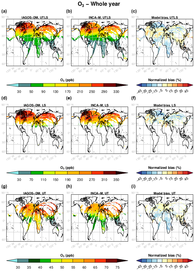
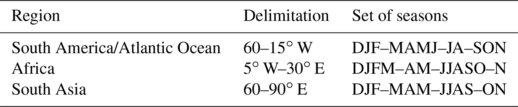
Figure 1Ozone mean horizontal distributions on yearly averages from December 1994 until November 2017 for the products IAGOS-DM (a, d, g) and INCA-M (b, e, h), as well as the biases (c, f, i) normalized with respect to the mean values between the two products. Each row displays a layer, with the non-separated UTLS at the top and the distinct LS and UT below.
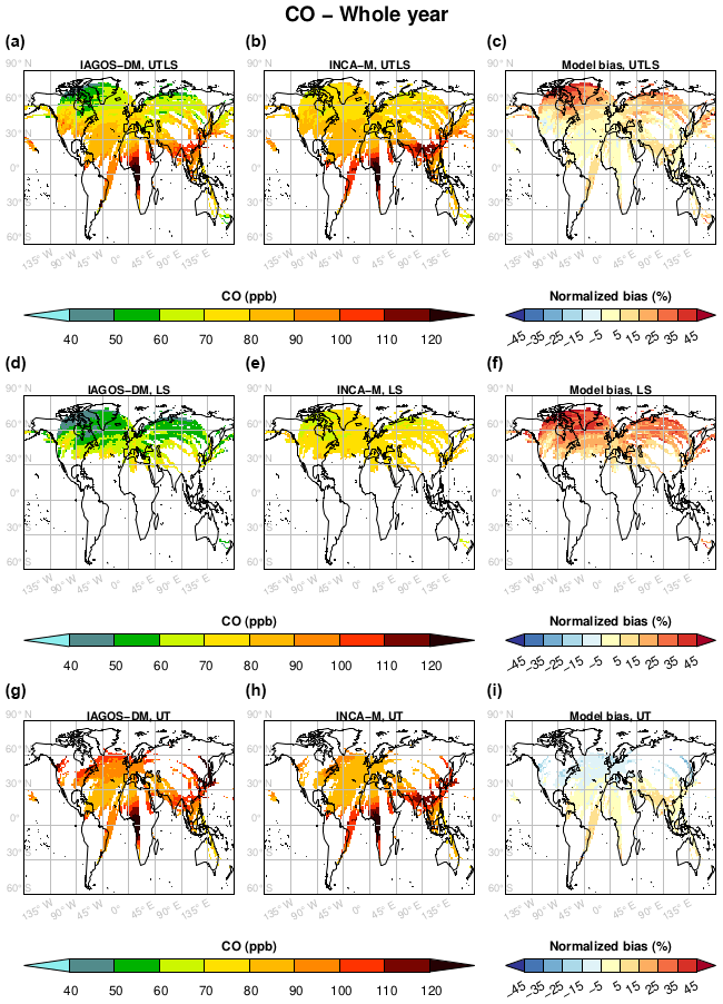
Figure 2Same as Fig. 1 for carbon monoxide from December 2001 until November 2017.
3.1 Horizontal distributions
Ozone, CO, NOy and water vapour yearly distributions in the UTLS, UT and LS are shown in Figs. 1–4, respectively, and their corresponding seasonal averages are available in the Supplement. They represent vertical averages through the cruise altitudes. Showing the results both with and without the separation is relevant because it can provide a better understanding for some biases visible in the UT or the LS. More generally, it is also relevant as a demonstration of the use of the Interpol-IAGOS software for both the simulations with and without an available potential vorticity field. Concerning the non-separated UTLS layer, it has to be noted that the vertical distribution of the IAGOS sampling relative to the tropopause level varies geographically, as a result of tropopause and cruise altitude variations. Consequently, the values shown in the UTLS layer are not considered representative of a geographically constant vertical domain, and they do not necessarily represent the whole transition layer. Also, it must be kept in mind that the UTLS layer is not solely the merging of the UT and the LS, since it also comprises the vertical range between 2 and 3 PVU that separates the two layers. Last, the altitude range of cruise measurements varies geographically as well. In the northern extratropics, the vertical range of the ozone measurements varies mostly between less than 1 km and up to 3 km, with a maximum frequency (∼ 40 %) between 1 and 2 km for the separated UT and LS and between 2 and 3 km for the non-separated UTLS.
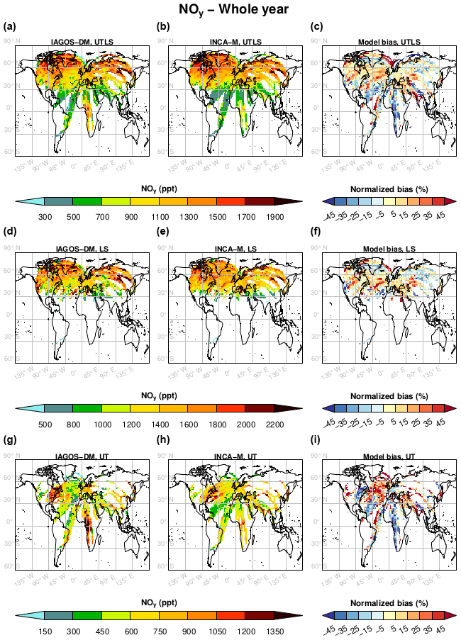
Figure 3Same as Fig. 1 for reactive nitrogen from December 1999 until November 2017.
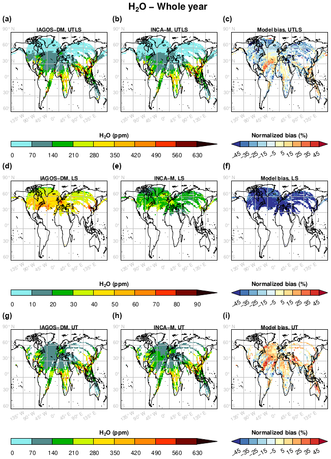
Figure 4Same as Fig. 1 for water vapour.
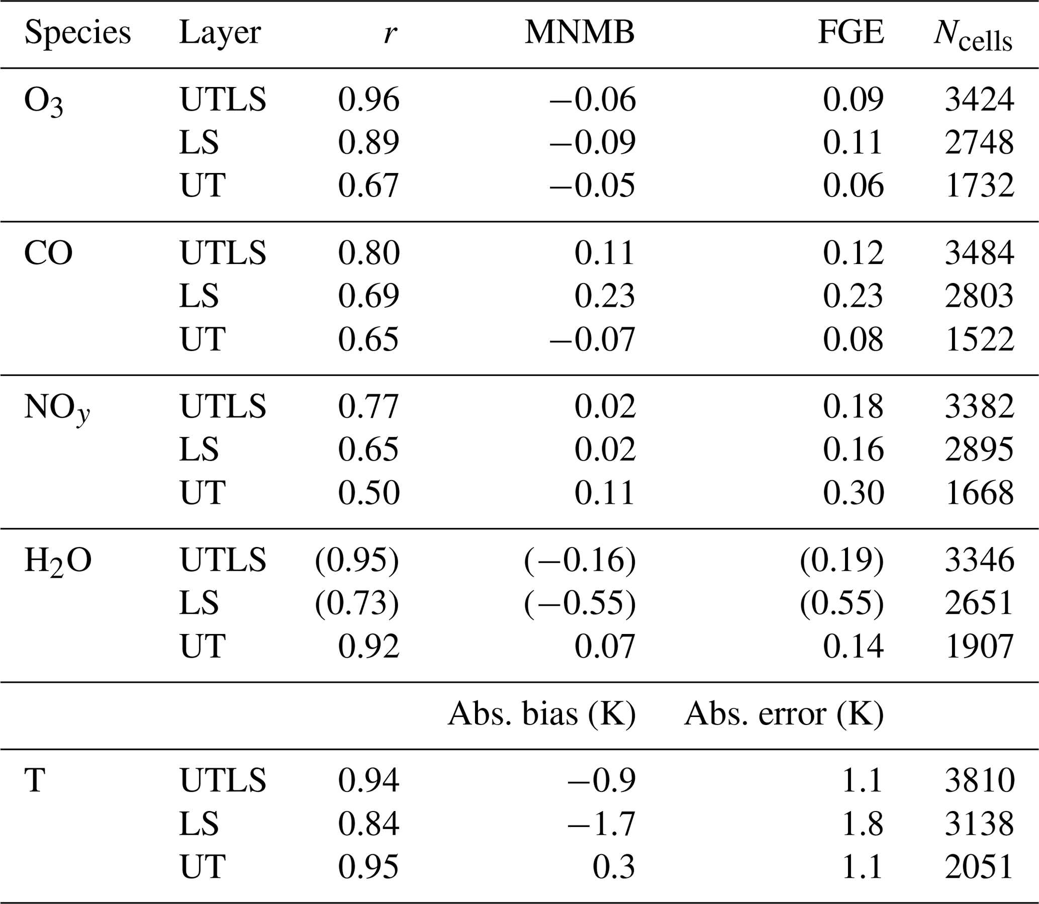
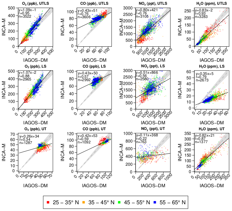
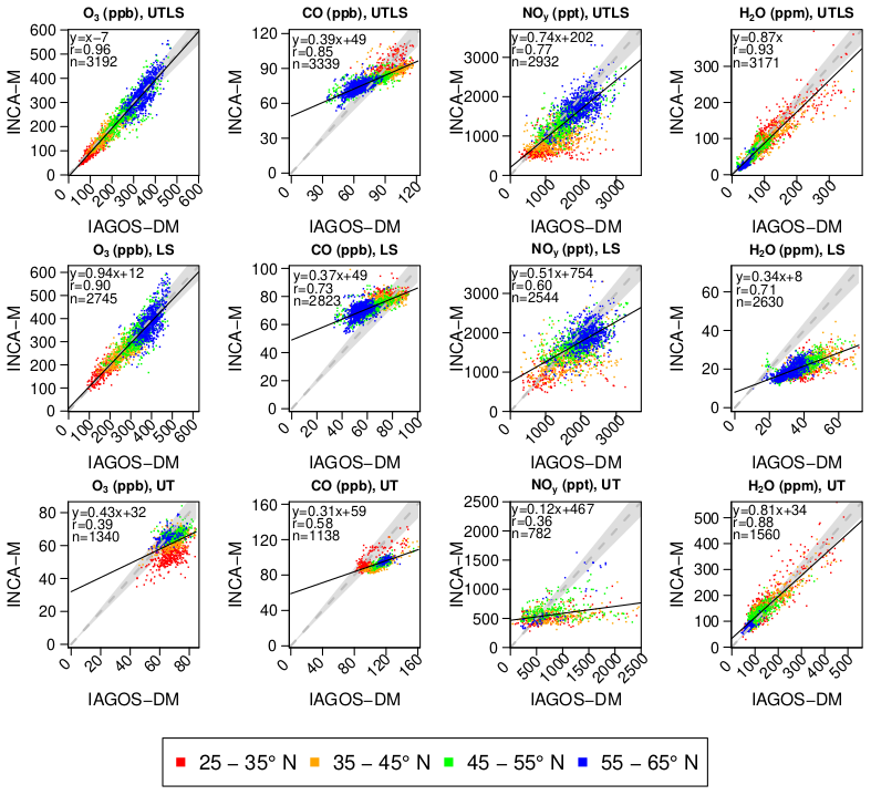
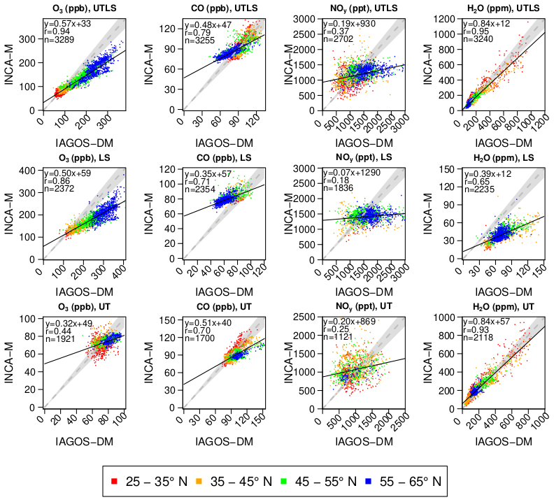
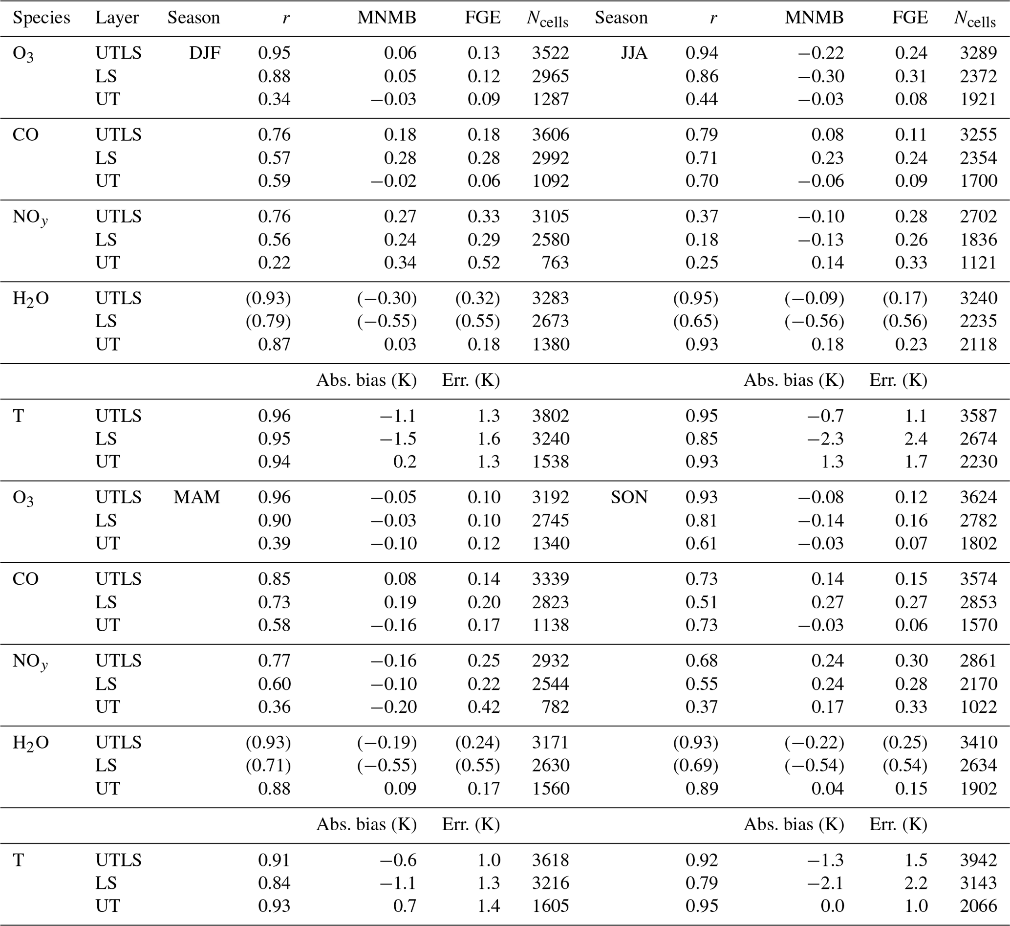
Table 2Annual metrics synthesizing the assessment of the O3, CO, NOy and H2O climatologies from the INCA-M core simulation against IAGOS-DM in several layers, as shown in Fig. 5. From left to right: Pearson's correlation coefficient (r), the modified normalized mean bias (MNMB), the fractional gross error (FGE) and the sample size (Ncells). As they cannot be used for the model assessment, the results for water vapour in the LS and in the mixed UTLS are represented in brackets. For the temperature, the absolute bias and its associated error are equivalent to the MNMB and the FGE without the normalizing factors.
Ozone climatologies (see Fig. 1) generally show geographical structures well reproduced by the model, i.e. the location of maxima in polar regions in the LS (west from Greenland and northern Siberia), the minimum in the western equatorial Pacific Ocean in the UT, and the transition between subtropical and extratropical areas. In addition, the corresponding ozone seasonal climatologies available in the Supplement show that each point highlighted in this paragraph is representative of three seasons at least. Figure 2 highlights similarities between the CO climatologies from the two data sets, like the good model reproduction of the extreme values above the (sub)tropical convective and strongly emitting regions. However, one of the main features in the extratropical latitudes remains an important overestimation of CO in the LS characterized by a smaller geographical variability and a moderate underestimation in the UT. The non-separated UTLS is relatively well reproduced in the mid-latitudes, with a moderate positive CO bias in the areas where the UT is not sampled, thus probably reflecting the lower-stratospheric positive bias. NOy is characterized by discrepancies between IAGOS-DM and INCA-M, especially in the UT with strong dipoles between positive and negative biases. The latter specificity is possibly an artefact due to the lower amount of measurements. Nevertheless, we identify collocated stratospheric footprints in the same polar regions as mentioned for ozone, an upper-tropospheric maximum above the eastern coast of North America and a noticeable minimum east of Central America. In the UT, the extratropical NOy tends to be overestimated, except the hot spot above the eastern coast of North America where NOy is underestimated. As for ozone, the H2O meridional variability shown in Fig. 4 is similar between the two data sets and particularly the delimitation of the area impacted by the Asian monsoon. The simulation catches the geographical H2O maxima above the most convective regions (equatorial lands and the area impacted by the Asian summer monsoon) and the maximum observed above the tropical Atlantic Ocean, as well as the collocated ozone minimum. This H2O feature is due to the westward extension of the central African peak advected by easterlies (Uma et al., 2014, Fig. 3). However, ozone and water vapour biases illustrate either the difficulty in parameterizing detrainment, notably from tropical convective systems (e.g. Folkins et al., 2006), or the phase of water. The latter depends on temperature but also on supersaturation, which is not implemented in the current model version, though it might represent an important fraction of the sampled air masses near the tropopause (Petzold et al., 2020). The LS is characterized by drier values in the model simulation, which is discussed later.
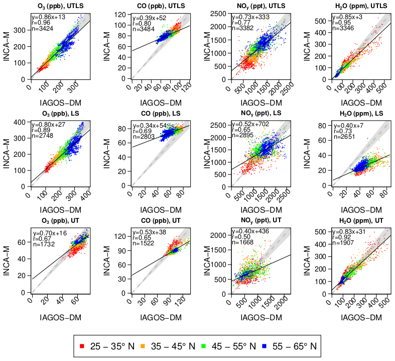
Figure 5Scatterplots representing the INCA-M yearly horizontal climatologies against the IAGOS-DM product in the latitudes beyond 25∘ N. Each row displays a layer, and each column displays a measured variable. Each colour represents a latitude band. For each graphic, the solid black line represents the linear regression fit described in the top-left corner with its equation, its Pearson correlation coefficient and the number of grid points involved in its calculation. The grey dashed line illustrates the y=x reference line, surrounded by a shaded ± 20 % margin. The outliers (outside the 1st and 99th percentiles) are not represented.
3.2 Northern extratropics
In this section, we propose a synthesis of the assessment in the UT, the LS and the mixed UTLS, followed by a sensitivity test with respect to the emissions from lightning and from biomass burning. As the tropics are sampled exclusively in the troposphere because of the higher tropopause altitude, we focus on the extratropics in order to derive metrics that characterize similar areas between the two layers. Figure 5 shows the scatterplots derived from Figs. 1–4 in the northern extratropics, with basic linear regression scores. Table 2 presents complementary metrics as the modified normalized mean bias (MNMB) and the fractional gross error (FGE) defined in Eqs. (1) and (2). For further detail, the seasonal scatterplots are shown in Figs. A1–A4, and the seasonal statistics are presented in Table A1. In this section, it is important to note that the values beyond the 1st and 99th percentiles are excluded from the calculations in order to prevent the scores from being influenced by the most extreme outliers. Concerning the water vapour measurements, it has to be noted that the IAGOS-Core sensor was not initially designed for air masses as dry as in the lower stratosphere and tends to have a wet bias for low RHL values. An additional filter was applied to IAGOS-DM as an attempt to make the LS data usable (see Sect. 2.3.2). However, the comparison between the model and the IAGOS-Core H2O data in the LS (and in the mixed UTLS) leads to the assumption that the filter was not sufficient, though the latter has been tested down to 5 % without visible changes in the MNMB or in the correlation. So, the IAGOS-Core H2O data cannot be used for model assessment, but at most they can be interpreted as an upper limit.
3.2.1 Model evaluation
According to Table 2, in the mixed UTLS, the core simulation exhibits high geographical correlations for ozone (r=0.96) and relatively high correlations for CO and NOy (r=0.80 and 0.77, respectively). It suggests that the variations in the tropopause altitude are realistically located in the nudged meteorological fields. The biases in the UTLS are rather negative for ozone and almost systematically positive for CO, and they show a wide variability for NOy. Table A1 shows that the annual biases in CO in the UTLS are representative of most seasons. Ozone has relatively small biases except in summer, when it is almost systematically negative. The NOy species are characterized by negative biases in spring and summer and by positive biases in fall and winter.
More details are provided with the UTLS splitting. For a given species, we note that there are high correlations between IAGOS-DM and INCA-M in the layer where the mixing ratios are at a maximum (LS for ozone; UT for water vapour; and, to a lesser extent, NOy in the LS). Except for ozone, the scores regarding biases show better results in the layer maximizing the mixing ratios, i.e. water vapour and CO in the UT and, though with an important variability, NOy in the LS. The negative bias in lower-stratospheric ozone is characterized by a strong and systematic negative bias in summer (MNMB = −0.30; FGE = 0.31), though with a good geographical correlation (r=0.86), and a systematic negative bias in temperature (−2.3 K). The latter suggests that the influence from the deeper stratosphere is underestimated during this season. On the contrary, good scores are visible for ozone during winter and spring (|MNMB|<0.06; FGE < 0.12; r≥0.90), suggesting that the impact of the Brewer–Dobson circulation on the LS is well represented. The diagnostics made in this study cannot be used for water vapour in the LS or in the UTLS, despite the filter applied to IAGOS-DM for this species. So far, the current tools used in this study only allow us to assess the model humidity in the UT.
Since their magnitudes are close to their respective FGE, the discrepancies mentioned for water vapour in the LS, ozone and CO display the same sign at most locations. The features concerning CO and NOy are representative of each season, except summertime NOy, which shows a very low correlation. Mostly representative of summer too, the model also shows more difficulties in simulating the NOy tropospheric features, especially in the 35–45∘ N band where high values are seen in the simulation only (Fig. A3). A comparison (not shown) with a climatology of observed lightning flash rates from the LIS–OTD database (Cecil et al., 2014) showed difficulties from the LMDZ-OR-INCA model in reproducing the lightning geographical distribution, with an important underestimation above marine grid cells and an overestimation above lands. These discrepancies are likely to play a significant role in the poor scores in the modelled NOy climatologies, especially during summer when the lightning activity is maximized (e.g. Holle et al., 2016). Uncertainties in aircraft emissions are also a potential source of important biases for this family of species in the LS, as the LMDZ-OR-INCA model response in NOy to the aviation emissions can reach more than 450 ppt in every season.
We note important biases in CO, systematically positive in the LS (MNMB = FGE = 0.23) with a poleward gradient well visible in Fig. 2 and low but negative at most locations in the UT (MNMB = −0.07; FGE = 0.08). As for lower-stratospheric ozone (MNMB = −0.09; FGE = 0.11), the sign of the biases is constant on almost all the sampled locations. Conversely for water vapour, the represented fraction of the UT is characterized by a positive bias more mitigated geographically (MNMB = 0.07; FGE = 0.14). Complementary information is provided in Table A1 with temperature scores well in phase with the water vapour discrepancies, i.e. a positive bias in the UT with a high geographical variability and an important correlation in the UT. As for water vapour, this description of the temperature behaviour is representative of most seasons. The saturating vapour pressure and the vertical stability as represented in the model might thus be an important factor in the water vapour discrepancies. However, the scores do not show the same seasonality between the two variables. The fact that supersaturation is not taken into account in the simulation is one possible reason for this behavioural difference.
In Fig. 5, we particularly note that the high correlations for ozone in both the UTLS (r=0.96) and the LS (r=0.89), as well as for water vapour in the UT (r=0.92), are characterized by a linear regression slope close to 1, thus showing a realistic geographical variability in these cases. Notably, the meridional structure highlighted with the colours is also well reproduced, and the LMDZ GCM captures well the large distribution of the water vapour mixing ratios at low latitudes (orange and red dots), spreading between dry subsiding and wet convective regions. These features concerning water vapour are representative of each season. On the contrary, the lower-stratospheric ozone variability is underestimated in summer and fall. The great scores shown in spring are consistent with a well-reproduced mean impact of the Brewer–Dobson circulation on the ozone mixing ratios, both in spatial distribution and in geographically averaged magnitude. In the UT, however, the colours show that the mean ozone northward gradient is overestimated. Carbon monoxide and reactive nitrogen have poorer scores, with lower correlation coefficients and a more underestimated geographical variability. Concerning NOy, the model reproduces the lower-stratospheric poleward gradient relatively well, probably due to the important quantities of stratospheric nitric acid, but hardly represents the variability inside each latitude band.
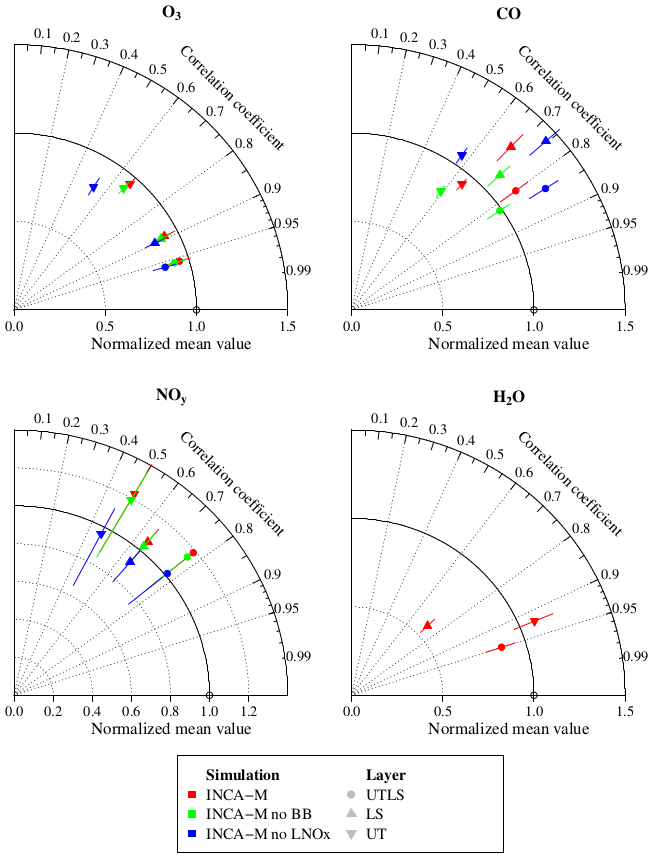
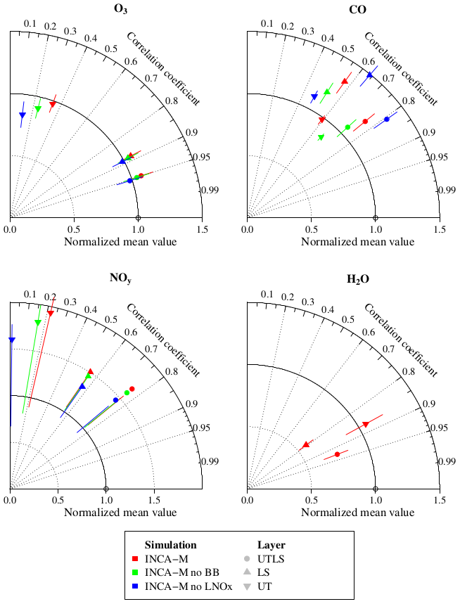
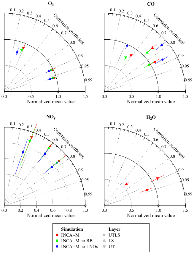
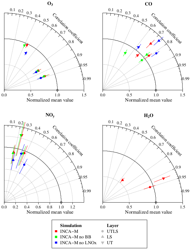
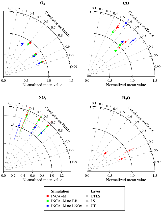
Figure 6Modified Taylor diagrams synthesizing the assessment of the yearly climatologies beyond 25∘ N derived from the three LMDZ-OR-INCA simulations against IAGOS-DM, for O3, CO, NOy and H2O. Each simulation is represented by a colour and each layer by a point shape. The radial axis corresponds to a normalized mean value. The orthoradial axis refers to the r correlation coefficient. The error bars are the quartiles 1 and 3 of the relative bias.
3.2.2 Comparison with the perturbation runs
The Taylor diagrams in Fig. 6 present a synthesis of the comparison between the reference run and the sensitivity runs, comprising a run without lightning emission (”No-LNOx”) and a run without biomass burning emissions (”No-BB”). The aim is the further understanding of the differences between the reference simulation and the observations and the further understanding of the observed climatologies when the reference run is consistent. In order to more clearly represent the differences between the runs, we chose to display the mean ratio (with its inter-quartile interval) of the model outputs to the observations. The advantage is keeping a constant denominator in the normalized mean values between the different simulations. Since modelled water vapour remains quasi-unchanged in the test, only the reference simulation is presented regarding this variable. First, the comparison between the different runs shows a better correlation in the reference simulation in the UT, implying that the impacts from lightning and biomass burning in the reference simulation contribute to a non-negligible part of the geographical similarities between IAGOS-DM and INCA-M. As expected, no change in the ozone correlation is observed in the LS. One possible reason is that the higher amounts of ozone in the LS increase the NOx threshold necessary to trigger a net ozone production (e.g. Hegglin et al., 2006). Another possible explanation is that ozone has a longer lifetime in the LS than in the troposphere: the impact of LNOx injections into the LS might thus be more homogeneous than in the UT, which would be consistent with the low sensitivity of the LS ozone geographical variability to lightning. Surprisingly, no important change in the correlation coefficients is obtained for NOy. This is consistent with the fact that areas where lightning emissions are the most abundant also maximize the convective uplift of surface pollutants into the UT. Also, the maximum above the northeastern American coast is consistent with the higher frequency in warm conveyor belts shown in Madonna et al. (2014). In contrast to NOy, the ozone correlation is sensitive to the removal of lightning sources (r=0.67 for the reference run, compared to r=0.53 for the run without lightning), suggesting that a part of the ozone distribution can be explained by the lightning distribution as represented in the model. Concerning CO, we can note a small loss of correlation in the UT without biomass burning or lightning but a small increase in the LS as well. While the loss of correlation is consistent for the UT, the gain in the LS may reveal an overestimated tropospheric influence on this layer, such as too much convection, which could also explain the water vapour positive bias in the UT.
The changes in biases are generally more important in the run without LNOx than without biomass burning. In the former run, ozone is decreased and shows an important negative bias (from −15 % to −20 % throughout the layers, in annual means), NOy is decreased and shows a small bias (between −10 % and 0 %), and CO is increased up to a 10 %–50 % positive bias due to decreased OH concentrations. The model thus overestimates the non-lightning NOy but not necessarily the NOx, as ozone is well underestimated in this simulation, assuming that the shorter period of time and the sparser measurements of NOy do not lead to strong differences. There are several possible explanations, including a lack of nitric acid (HNO3) loss by scavenging in the troposphere and/or heterogeneous reactions. The lack of scavenging combined with the overestimation of the cross-tropopause exchanges would be consistent with the non-lightning NOy overestimation in all the layers.
As expected, the impact of biomass burning emissions on the biases is weak for ozone and reactive nitrogen, whatever the season. In the run with no biomass burning, we observe decreases in CO, and the annual model CO bias changes from −5 % to −15 % in the UT, from 30 % to 15 % in the LS and from 15 % to 0 % in the UTLS. Surprisingly, the impact of biomass burning is not negligible in the LS, especially in the summer. It is likely that the influence of biomass burning on the LS is overestimated because of an excessive exchange between the troposphere and the stratosphere. The change in correlation linked to biomass burning emissions is mainly visible in the upper-tropospheric CO and is mainly representative of summer, when the r coefficient drops from 0.70 to 0.50. This suggests that this season maximizes the impact of biomass burning in the UT as it contributes significantly to the CO distribution, and it is consistent with the important summertime maxima in CO emissions from boreal forests in both the GFAS and GFED inventories (Andela et al., 2013).
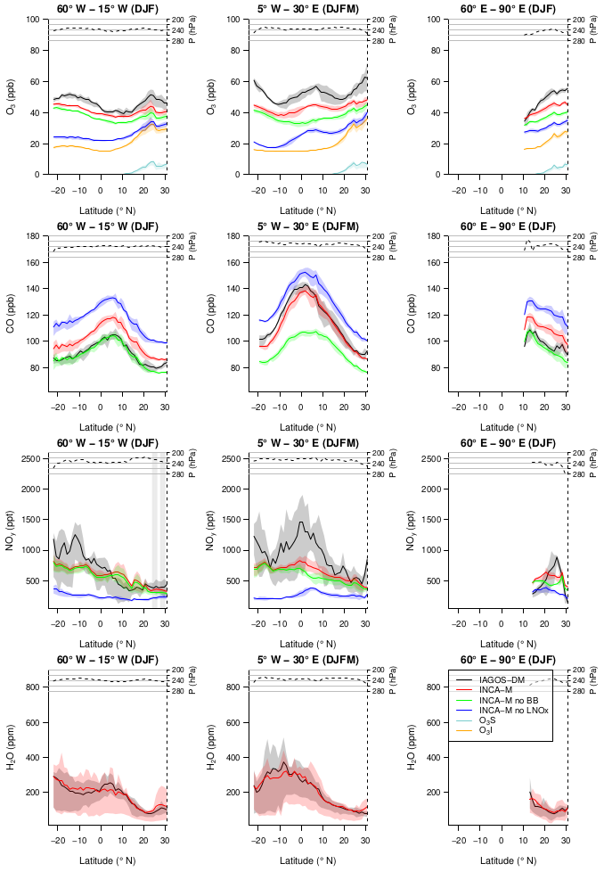
Figure 7Zonal cross sections between 25∘ S and 30∘ N from December until February or March. Each row represents a measured variable, and each column represents a longitude interval from which the zonal means have been derived. As the season's definition, they are indicated in the title of each graphic. The uncertainties shown here correspond to the spatial variability, defined as the interval between the quartiles 1 and 3. The solid black line corresponds to IAGOS-DM, whereas the red, blue and green lines correspond, respectively, to the INCA-M reference simulation and to the INCA-M simulations without emissions from lightning and from biomass burning. In the ozone panels, the orange and light-blue lines show the O3I and O3S stratospheric tracers. The dashed line at the top of each graphic shows the mean pressure derived from observations. The latter's values are reported on the right axis.
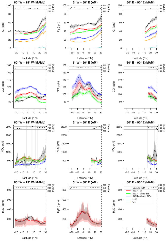
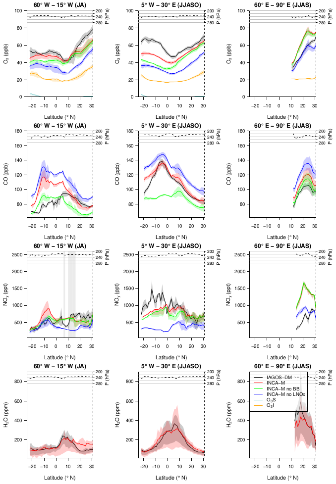
Figure 9Same as Fig. 7 for July–August, June–October and June–September, from left to right.
3.3 Tropics
Figures 7–10 compare the zonal cross sections in the tropics derived from IAGOS-DM and the three INCA-M simulations during the four seasons defined in Table 1. The profiles were derived from averages along both the vertical and longitudinal axes, using the upper-tropospheric grid cells only. The mean pressures on the right axis have been added in order to identify changes in mean altitude measurements. They can be associated with significant changes at the edges of the sampled region or with a change in the width of the longitude interval. This case mainly corresponds to NOy measurements during November above southern Africa and October–November above South Asia. The corresponding profile shapes are thus difficult to interpret, but the comparison with the model remains valuable. Given the negligible changes in water vapour from one simulation to another, we only show its reference simulation profiles, as in Fig. 6. Last, with a lessened sampling efficiency and a shorter measurement time period for NOy, the comparison between its profiles and the ozone profiles is not necessarily relevant. We thus performed a representativeness test on ozone, projecting only the IAGOS data characterized by a valid NOy measurement. The points where the subsequent difference with the reference ozone profiles is greater than 10 % are indicated with shaded areas in the NOy panels. Their small number of occurrences indicates that seasonal mean ozone does not vary much between the two periods and/or sampling modes, which provides more confidence regarding the representativeness of the NOy measurements in the context of the whole ozone measurement period.
3.3.1 Observed features
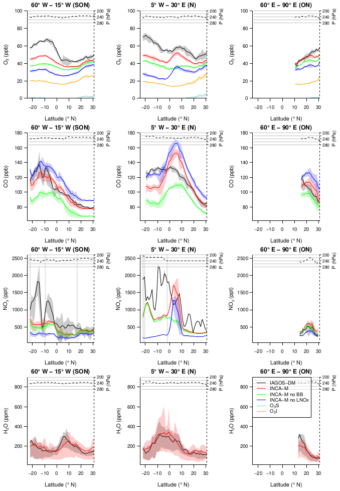
Before assessing the model, it is worth presenting the main features exhibited by the observations and proposing some explanation, with a focus on the most complete profiles (Atlantic and Africa). The water vapour maxima are collocated with ozone minima during the northern monsoon seasons (JA and JJASO for the Atlantic and Africa, respectively), representing the most convective areas. Above Africa, in both southern and northern monsoons, Sauvage et al. (2007b) and Lannuque et al. (2021) attributed the ozone gradients surrounding the minimum to the uplift of precursors in the ITCZ, leading to increased photochemical activity during the poleward transport. This is consistent with the peak in the modelled net ozone production efficiency (not shown) that surrounds these ozone minima. In the same continent, the CO maximum is shifted from the water vapour peak. The same study showed that the CO emitted at the surface, notably from the dry areas where biomass burning activity is increased, was uplifted into the ITCZ, was transported poleward in the Hadley cell upper branch and accumulated in the vicinity of increased wind shear areas. Above Atlantic–South America, CO is maximized during SON. Livesey et al. (2013) showed similar results using MLS measurements around 215 hPa from 2004 until 2011, with more significant seasonal cycles above the South American tropics and subtropics. They also show this corresponds to the transition season between the continental dry and wet seasons. The southern CO maximum that we observe here is thus due to the start of an enhanced convective activity while biomass burning emissions are still intense. Among the three regions, tropical Africa shows the most important CO maxima. The only season with comparable peaks between Africa and South America is September–November, and the southern part from 15∘ S is not likely to be influenced by African emissions, as Yamasoe et al. (2015) showed that these latitudes were characterized by westerly winds during this season. The Asian summer monsoon maximizes the water vapour mixing ratios, reaching 600 ppm against almost 400 ppm above Africa and 300 ppm above South America. This regional maximum may be explained by higher temperatures (∼ +5 K) that allow a more abundant gaseous phase (not shown), probably due to the particularly strong wet convection. One could expect the CO mixing ratio to be more important in the UT above the Asian summer monsoon, as shown from the Infrared Atmospheric Sounding Interferometer (IASI) satellite data in Barret et al. (2016), with surface tracers accumulating in the associated anticyclone. However, the altitude range observed in Barret et al. (2016) where CO is more abundant in the Asian summer monsoon spreads from 270 up to 110 hPa, thus partially higher than the IAGOS cruise data. It is therefore likely that the higher tropopause altitude characterizing the Asian summer monsoon system (e.g. Fig. 9d in Li et al., 2017) leads to an elevated CO vertical maximum that the IAGOS aircraft cannot sample, as Park et al. (2009) showed a vertical maximum near 15 km inside the anticyclone. In this region, ozone and reactive nitrogen reach their seasonal maxima during March–May, correlated with the lower-stratospheric ozone maximum in the mid-latitudes due to the Brewer–Dobson circulation. This is consistent with enhanced ozone stratosphere-to-troposphere transport during the pre-monsoon season, as shown by Barret et al. (2016) and as suggested by the large seasonal ratio highlighted in this region by Cohen et al. (2018); this was also confirmed with measurements from the High Altitude and Long Range Research Aircraft (HALO) during the HALO-ESMVal campaign in 2012 (Gottschaldt et al., 2018) showing correlated enhancements of hydrochloric acid (HCl) and ozone. This seasonal maximum is then interrupted by the northward shift of the subtropical jet during the monsoon that confines the stratospheric intrusions to the northern side of the Himalayas (Cristofanelli et al., 2010). The strong northward ozone gradient in the monsoon season is consistent with the northward transport of air masses with a seasonally maximized net ozone production (not shown), as simulated in Gottschaldt et al. (2018) also. They linked such important photochemical activity with a combination of uplifted precursors from the surface and lightning NOx emissions, though the latter were shown reaching their maximum during the previous season.
3.3.2 Model assessment
Good consistency between the reference simulation and the observations is visible for ozone, CO and water vapour. The latter is the species with the best consistency, with the smallest bias at most latitudes and during most seasons. Above the Atlantic, during the North American summer monsoon (Fig. 9), the model reproduces the H2O maximum at 5–10∘ N well but not the drop at the northern side, leading to strong relative biases along the northern tropic (75 ppm on average, thus 65 % of the observed mixing ratio). We also note that the model tends to underestimate the latitudinal variability in this region, especially from March until June (Fig. 8) when it is quasi-absent in the simulation. Above Africa, the model captures well the width and the magnitude of the maximum. Above South Asia, the simulation has difficulties in reproducing the extremely high water vapour mixing ratios during the monsoon season on average (−110 ppm bias, thus −20 %). Nevertheless, water vapour remains simulated with higher amounts in the UT above the Asian summer monsoon than above the other regions. Despite these significant biases, the overall consistency in water vapour profiles suggests that the transport in the nudged simulation is reliable and can accurately reproduce some convective features, even in the monsoon systems.
Ozone is almost systematically underestimated in the reference simulation, but its variations are mostly in agreement with the observations, with collocated extrema and similar meridional gradients. The stratospheric ozone tracer (O3S) indicates very low values: systematically less than 5 ppb except during the DJF/DJFM season when it plays the main role in the northward ozone gradient north of 15–20∘ N. However, we note an underestimated northward gradient in the northern subtropics, especially during the March–May season. Though this season maximizes the stratosphere-to-troposphere transport as explained in the previous paragraphs, the O3S tracer shows low mixing ratios, which highlights an underestimated impact from the stratospheric intrusions. The inert stratospheric ozone tracer (O3I), instead, follows a stronger gradient in this area. The underestimation of the stratospheric influence in INCA-M may thus be explained by an underestimation of the ozone lifetime in these areas and seasons. Carbon monoxide tends to be overestimated, except above Africa from December to March and from June to October when the profiles are particularly well reproduced, combining good correlations and small biases. In most regions and seasons, the simulation shows a consistent variability in CO despite some cases where the profiles are poorly correlated with the observations (mainly the MAMJ and JA seasons over the Atlantic Ocean). The model reproduces the higher maximum CO mixing ratios in tropical Africa well compared to the other two areas. The simulated NOy profiles underestimate the observed meridional variability. Above Africa, NOy is almost systematically underestimated by the model in the Southern Hemisphere, but the NOy comparisons show a general consistency in the Northern Hemisphere. Last, we note an important positive NOy bias during the Asian summer monsoon (more than +100 % on average) that is further characterized later using the other two simulations.
3.3.3 Comparison with the perturbation runs
As expected, the lightning emissions have a stronger contribution to upper-tropospheric ozone compared to biomass burning, as suggested by a similar behaviour for NOy. Though the source strengths are comparable, the important contribution from lightning to the NOx injection at these altitudes leads to a greater ozone production efficiency, compared to other sources (Sauvage et al., 2007a). Notably, the Atmospheric Chemistry and Climate Model Intercomparison Project (ACCMIP) models estimated the ozone production efficiency from lightning to be 6.5 ± 4.7 times greater than from the other sources (Finney et al., 2016). Lightning emissions also contribute significantly to the meridional gradients in ozone and NOy north and south of the ITCZ, as the difference between the reference and the no-LNOx simulations shows some strong variability. As expected, the role of lightning NOx in CO destruction mostly consists of a background signal involving NOx emissions that enhance both ozone and OH production, with ozone itself acting as a source of OH in presence of water vapour. The increased OH mixing ratios finally destroy CO with an average lifetime of 38 d in the tropics (Lelieveld et al., 2016). The CO chemical destruction is thus a slow process compared to zonal transport, which can explain the spread pattern of the sensitivity to LNOx emissions. Some geographical differences in the impacts of lightning on CO are still visible, notably between the opposite subtropics, probably reflecting a slow interhemispheric transport.
Some ozone discrepancies can be explained by the combined comparison between species and between simulations. For example, the ozone and CO local maxima simulated near 5–10∘ S over Africa in April–May are not visible in the observations. This increase remains visible in the no-LNOx simulation but not in the no-BB simulation. It is particularly visible in the CO profiles, characterized by an exaggerated peak collocated with the ozone local maximum. The impact of biomass burning is therefore overestimated in the model over this area during April–May. A similar feature is highlighted in November above Africa, where a peak in NOy is seen only by the model and arises from biomass burning. This overestimation in biomass burning products contributes to a collocated steep peak in CO, whereas the observations show a flat maximum, and to an ozone local maximum, while it is barely visible in the observations. Since even the no-BB simulation exhibits a peak in CO that contrasts with the IAGOS-DM flat maximum, the convection parameterization and/or the anthropogenic emission inventory may play a role in this overestimated spatial variability. Last, one noticeable ozone discrepancy takes place during the Asian summer monsoon, when the bias reaches +20 ppb. The NOy profiles allow us to point out the excessively high modelled value, reaching more than twice the observed mixing ratios. It is interesting to note that even without LNOx, NOy remains overestimated and ozone becomes more consistent with the observed profile. Since the impact of lightning activity during this monsoon on ozone production is well established (e.g. Gottschaldt et al., 2018), it suggests either an overestimated transport from the boundary layer or an underestimated washout of soluble species like HNO3.
These sensitivity tests also allow us to associate significant contributions with several well-reproduced features. Above South America–Atlantic Ocean, the CO maximum during SON between 5 and 15∘ S has a non negligible contribution from local biomass burning (∼ 20 ppb, thus ∼ 10 ppb more than in other latitudes), consistent with the literature (notably Livesey et al., 2013; Tsivlidou et al., 2023). The lightning contribution to the ozone maximum between 5 and 15∘ S is in agreement with the GEOS-Chem model used in Yamasoe et al. (2015). The next season (DJF) is characterized by a well-correlated CO profile, although positively biased, and the model associates the 5∘ S–15∘ N maximum with other sources. During the summer monsoon above Africa, the CO peak above 0–10∘ S is associated with local biomass burning emissions, as is a significant part of the peak above 5∘ S–5∘ N during the opposite season (DJFM). In contrast, the observed CO maximum during April–May between 5 and 10∘ N is rather associated with other sources. These features are in agreement with the results presented in Lannuque et al. (2021) based on the SOFT-IO source-apportionment software (Sauvage et al., 2017). According to the model, an important part of the differences in CO between tropical Africa and the other two regions is mainly caused by biomass burning. Above South Asia, CO is less influenced by biomass burning during the monsoon season, consistent with the literature. For example, Jiang et al. (2007) attributed most of upper-tropospheric CO levels to anthropogenic emissions, because of deep convection that both uplifts surface pollution into the UT and reduces wildfires via enhanced precipitation.
This study presents an assessment of a long-term simulation from the LMDZ-OR-INCA chemistry–climate model (CCM) with daily resolved outputs in the upper troposphere–lower stratosphere (UTLS). More precisely, we evaluate ozone, carbon monoxide (CO), reactive nitrogen (NOy) and water vapour climatologies based on all of the cruise IAGOS data set including the IAGOS-CARIBIC data, respectively, during the periods December 1994–November 2017, December 2001–November 2017, December 1999–November 2017 and December 1994–November 2017.
In order to allow a direct comparison between the simulation output and the high-resolution IAGOS data sets, we use the Interpol-IAGOS software that projects the IAGOS data onto the model grid (Cohen et al., 2021). As a first step, we extend this tool to daily model outputs. The subsequent IAGOS product (IAGOS-DM) is generated by interpolating the IAGOS data onto the model grid and then deriving weighted monthly averages on each grid cell. Similar to IAGOS-DM, the product based on the simulation output (INCA-M) is also made of monthly averages across the sampled daily grid points only. As a second step, we compare the annual and seasonal climatologies derived from these two products. The assessment in the mid-latitudes is made separately in the upper troposphere (UT) and the lower stratosphere (LS) using the model potential vorticity (PV) but also in the UTLS like in a single layer, as an option for the models that do not sort out the potential vorticity. In the tropics, the assessment only accounts for upper-tropospheric air masses because of the higher tropopause altitude.
In the northern mid-latitudes, the LMDZ-OR-INCA model exhibits good skills for ozone in the LS and for water vapour in the UT. The seasonal scores show that the influence from the deeper stratosphere on the LS through the Brewer–Dobson circulation is well modelled. At most locations, ozone is slightly underestimated by the model in the UT, and model CO shows a positive bias in the LS and a slight negative bias in the UT. These features suggest an overestimation in the model's extratropical cross-tropopause net transport. The bias in reactive nitrogen shows an important geographical variability in every layer. This is likely linked with the difficulty in reproducing the lightning geographical distribution but also with aircraft emissions, as shown by some biases in the shape of tracks. The latter can play a significant role in NOy levels. For example, the model intercomparison presented in Olsen et al. (2013) shows an aviation NOy perturbation ranging from 15 % to 40 % of the NOy level at the cruise altitudes, suggesting an important sensitivity to aircraft emissions. Another possible cause for the NOy discrepancies is the uncertainty in the scavenging processes for soluble species like HNO3 during their upward transport. Last, concerning water vapour in the LS, the IAGOS-Core humidity sensor was initially designed for tropospheric air masses. Though a filter has been applied in an attempt to exclude most of the measurements likely to overestimate the humidity, the corresponding climatologies in the LS shown in this study still cannot be used to assess the model simulation. One possible explanation is that the filtering method makes the IAGOS H2O mean values only representative of particularly moist conditions (on a sub-daily scale), thus increasing substantially the difference with the model output.
In the tropics and subtropics, the mean zonal cross sections are generally in good agreement between the model and the observations for ozone, CO and especially for water vapour. The latter shows that the LMDZ model, nudged into the ERA-Interim reanalysis, is able to accurately represent the mean transport features, notably the water vapour geographical maximum in the Asian summer monsoon. CO is well represented in the regions and seasons characterized by important contributions from biomass burning, i.e. during the convective season above South America (September–November), as well as above Africa for the seasons with the southernmost (December–March) and the northernmost (June–October) shifts of the ITCZ. In these cases, the model attributes, respectively, 25, 30 and 45 ppb of the CO peaks to biomass burning and attributes between 10 and 20 ppb of the CO sink to lightning emissions. The latter enhances the CO destruction by increasing the ozone production, which in turn increases the OH production. Though ozone is generally underestimated, the extrema locations and the meridional gradients are consistent with the observations in most seasons and longitude domains. It is mostly sensitive to lightning emissions of nitrogen oxides (LNOx), which can contribute up to a half of the modelled ozone in the Southern Hemisphere during the first half of the year. On the other hand, the biomass burning contribution to modelled ozone reaches 20 %–25 % where enhanced CO is attributed to biomass burning peaks.
Some of the inconsistencies in model ozone and CO with respect to the observations are linked to biomass burning emissions. Consequently, improvements in the biomass burning emissions or convection up to the UT are likely to enhance the model skills for CO and, to a lesser extent, for ozone. Also, though lightning as represented in the model helps in understanding the ozone geographical distribution, improving the lightning parameterization is likely to lead to the enhancement of the model skills for NOy and ozone.
As demonstrated through this paper, the new version of the Interpol-IAGOS software allows a multi-species assessment for modelled climatologies in the separated UT and LS, or in the UTLS as a whole, by using either the model daily output or the model monthly output (Cohen et al., 2021). It can easily be applied to a wide range of long-term simulations, notably in multi-model experiments. Concerning the latter, two applications are currently in progress in the framework of the second phase of the Tropospheric Ozone Assessment Report (TOAR-II) and of the ACACIA EU project (Advancing the Science for Aviation and Climate) and will be published elsewhere. Other potential applications include the assessment of modelled time series on regional scales and, for interannual variability and long-term trends, possibly also allowing for source apportionment regarding the observed features.

The IAGOS data (IAGOS, 2022) are available at the IAGOS data portal (https://doi.org/10.25326/20, Petzold et al., 2015a), and, more precisely, the time series data are found at https://doi.org/10.25326/06 (Boulanger et al., 2018). The Interpol-IAGOS software is available at https://doi.org/10.25326/81 (Cohen et al., 2020).
The supplement related to this article is available online at: https://doi.org/10.5194/acp-23-14973-2023-supplement.
YC designed the study, with advice from DH and BS. The Interpol-IAGOS software was further developed by YC. The simulation outputs were provided by YC and DH. The IAGOS data were provided by VT, AP, SR, UB, AZ and HZ. PK and SR provided important advice on the use of the water vapour data and DH on the use of the model. The paper was written by YC and reviewed, commented, edited and approved by all the authors.
At least one of the (co-)authors is a member of the editorial board of Atmospheric Chemistry and Physics. The peer-review process was guided by an independent editor, and the authors also have no other competing interests to declare.
Publisher's note: Copernicus Publications remains neutral with regard to jurisdictional claims made in the text, published maps, institutional affiliations, or any other geographical representation in this paper. While Copernicus Publications makes every effort to include appropriate place names, the final responsibility lies with the authors.
The authors acknowledge the strong support of the European Commission, Airbus and the airlines (Lufthansa, Air France, Austrian Airlines, Air Namibia, Cathay Pacific, Iberia and China Airlines so far) who have carried the IAGOS-Core equipment and performed the maintenance since 1994. In its last 10 years of operation, IAGOS-Core has been funded by INSU–CNRS (France), Météo-France, Université Paul Sabatier (Toulouse, France) and Forschungszentrum Jülich (FZJ, Jülich, Germany). IAGOS has been additionally funded by the EU projects IAGOS-DS and IAGOS-ERI. The IAGOS-Core database is supported by AERIS. Data are also available on the AERIS website http://www.aeris-data.fr (last access: November 2022). The simulations were performed using HPC resources from GENCI (Grand Équipement National de Calcul Intensif) under the gen2201 project. We also wish to acknowledge our colleagues from the IAGOS teams in FZJ, LAERO, DLR and KIT for all the preparation of the IAGOS and CARIBIC data used in this study, as well as the colleagues in LSCE for the training on the use of the modelling tools.
This research has been funded by the European Union Horizon 2020 research and innovation programme under the STRATOFLY (grant agreement no. 769246) and ACACIA (grant agreement no. 875036) projects, and by the French Ministère de la Transition écologique et Solidaire (grant no. DGAC 382 N2021-39), with support from France’s Plan National de Relance et de Résilience (PNRR) and the European Union’s NextGenerationEU.
This paper was edited by Jerome Brioude and reviewed by two anonymous referees.
Allen, D., Pickering, K., Duncan, B., and Damon, M.: Impact of lightning NO emissions on North American photochemistry as determined using the Global Modeling Initiative (GMI) model, J. Geophys. Res.-Atmos., 115, D22301, https://doi.org/10.1029/2010JD014062, 2010. a
Andela, N., Kaiser, J., Heil, A., van Leeuwen, T. T., Wooster, M. J., van der Werf, G. R., Remy, S., and Schultz, M. G.: Assessment of the Global Fire Assimilation System (GFASv1), ECMWF, 72 pp., https://doi.org/10.21957/7pg36pe5m, 2013. a
Arias, P., Bellouin, N., Coppola, E., Jones, R., Krinner, G., Marotzke, J., Naik, V., Palmer, M., Plattner, G.-K., Rogelj, J., Rojas, M., Sillmann, J., Storelvmo, T., Thorne, P., Trewin, B., Achuta Rao, K., Adhikary, B., Allan, R., Armour, K., Bala, G., Barimalala, R., Berger, S., Canadell, J., Cassou, C., Cherchi, A., Collins, W., Collins, W., Connors, S., Corti, S., Cruz, F., Dentener, F., Dereczynski, C., Di Luca, A., Diongue Niang, A., Doblas-Reyes, F., Dosio, A., Douville, H., Engelbrecht, F., Eyring, V., Fischer, E., Forster, P., Fox-Kemper, B., Fuglestvedt, J., Fyfe, J., Gillett, N., Goldfarb, L., Gorodetskaya, I., Gutierrez, J., Hamdi, R., Hawkins, E., Hewitt, H., Hope, P., Islam, A., Jones, C., Kaufman, D., Kopp, R., Kosaka, Y., Kossin, J., Krakovska, S., Lee, J.-Y., Li, J., Mauritsen, T., Maycock, T., Meinshausen, M., Min, S.-K., Monteiro, P., Ngo-Duc, T., Otto, F., Pinto, I., Pirani, A., Raghavan, K., Ranasinghe, R., Ruane, A., Ruiz, L., Sallée, J.-B., Samset, B., Sathyendranath, S., Seneviratne, S., Sörensson, A., Szopa, S., Takayabu, I., Tréguier, A.-M., van den Hurk, B., Vautard, R., von Schuckmann, K., Zaehle, S., Zhang, X., and Zickfeld, K.: Technical Summary, 33–144, Cambridge University Press, Cambridge, United Kingdom and New York, NY, USA, https://doi.org/10.1017/9781009157896.002, 2021. a
Barret, B., Sauvage, B., Bennouna, Y., and Le Flochmoen, E.: Upper-tropospheric CO and O3 budget during the Asian summer monsoon, Atmos. Chem. Phys., 16, 9129–9147, https://doi.org/10.5194/acp-16-9129-2016, 2016. a, b, c
Blot, R., Nedelec, P., Boulanger, D., Wolff, P., Sauvage, B., Cousin, J.-M., Athier, G., Zahn, A., Obersteiner, F., Scharffe, D., Petetin, H., Bennouna, Y., Clark, H., and Thouret, V.: Internal consistency of the IAGOS ozone and carbon monoxide measurements for the last 25 years, Atmos. Meas. Tech., 14, 3935–3951, https://doi.org/10.5194/amt-14-3935-2021, 2021. a
Bojinski, S., Verstraete, M., Peterson, T. C., Richter, C., Simmons, A., and Zemp, M.: The Concept of Essential Climate Variables in Support of Climate Research, Applications, and Policy, B. Am. Meteorol. Soc., 95, 1431–1443, https://doi.org/10.1175/BAMS-D-13-00047.1, 2014. a
Boulanger, D., Blot, R., Bundke, U., Gerbig, C., Hermann, M., Nédélec, P., Rohs, S., and Ziereis, H.: IAGOS time series, AERIS [data set], https://doi.org/10.25326/06, 2018. a
Brenninkmeijer, C. A. M., Crutzen, P. J., Fischer, H., Güsten, H., Hans, W., Heinrich, G., Heintzenberg, J., Hermann, M., Immelmann, T., Kersting, D., Maiss, M., Nolle, M., Pitscheider, A., Pohlkamp, H., Scharffe, D., Specht, K., and Wiedensohler, A.: CARIBIC–Civil Aircraft for Global Measurement of Trace Gases and Aerosols in the Tropopause Region, J. Atmos. Ocean Tech., 16, 1373–1383, https://doi.org/10.1175/1520-0426(1999)016<1373:CCAFGM>2.0.CO;2, 1999. a
Brenninkmeijer, C. A. M., Crutzen, P., Boumard, F., Dauer, T., Dix, B., Ebinghaus, R., Filippi, D., Fischer, H., Franke, H., Frieß, U., Heintzenberg, J., Helleis, F., Hermann, M., Kock, H. H., Koeppel, C., Lelieveld, J., Leuenberger, M., Martinsson, B. G., Miemczyk, S., Moret, H. P., Nguyen, H. N., Nyfeler, P., Oram, D., O'Sullivan, D., Penkett, S., Platt, U., Pupek, M., Ramonet, M., Randa, B., Reichelt, M., Rhee, T. S., Rohwer, J., Rosenfeld, K., Scharffe, D., Schlager, H., Schumann, U., Slemr, F., Sprung, D., Stock, P., Thaler, R., Valentino, F., van Velthoven, P., Waibel, A., Wandel, A., Waschitschek, K., Wiedensohler, A., Xueref-Remy, I., Zahn, A., Zech, U., and Ziereis, H.: Civil Aircraft for the regular investigation of the atmosphere based on an instrumented container: The new CARIBIC system, Atmos. Chem. Phys., 7, 4953–4976, https://doi.org/10.5194/acp-7-4953-2007, 2007. a
Brunner, D., Staehelin, J., and Jeker, D.: Large-scale nitrogen oxide plumes in the tropopause region and implications for ozone, Science, 282, 1305–1309, https://doi.org/10.1126/science.282.5392.1305, 1998. a
Brunner, D., Staehelin, J., Rogers, H. L., Köhler, M. O., Pyle, J. A., Hauglustaine, D., Jourdain, L., Berntsen, T. K., Gauss, M., Isaksen, I. S. A., Meijer, E., van Velthoven, P., Pitari, G., Mancini, E., Grewe, G., and Sausen, R.: An evaluation of the performance of chemistry transport models by comparison with research aircraft observations. Part 1: Concepts and overall model performance, Atmos. Chem. Phys., 3, 1609–1631, https://doi.org/10.5194/acp-3-1609-2003, 2003. a, b
Brunner, D., Staehelin, J., Rogers, H. L., Köhler, M. O., Pyle, J. A., Hauglustaine, D. A., Jourdain, L., Berntsen, T. K., Gauss, M., Isaksen, I. S. A., Meijer, E., van Velthoven, P., Pitari, G., Mancini, E., Grewe, V., and Sausen, R.: An evaluation of the performance of chemistry transport models - Part 2: Detailed comparison with two selected campaigns, Atmos. Chem. Phys., 5, 107–129, https://doi.org/10.5194/acp-5-107-2005, 2005. a, b
Cecil, D. J., Buechler, D. E., and Blakeslee, R. J.: Gridded lightning climatology from TRMM-LIS and OTD: Dataset description, Atmos. Res., 135–136, 404–414, https://doi.org/10.1016/j.atmosres.2012.06.028, 2014. a, b
Cohen, Y., Petetin, H., Thouret, V., Marécal, V., Josse, B., Clark, H., Sauvage, B., Fontaine, A., Athier, G., Blot, R., Boulanger, D., Cousin, J.-M., and Nédélec, P.: Climatology and long-term evolution of ozone and carbon monoxide in the upper troposphere–lower stratosphere (UTLS) at northern midlatitudes, as seen by IAGOS from 1995 to 2013, Atmos. Chem. Phys., 18, 5415–5453, https://doi.org/10.5194/acp-18-5415-2018, 2018. a
Cohen, Y., Thouret, V., Marécal, V., and Josse, B.: Interpol-IAGOS software, AERIS [code], https://doi.org/10.25326/81, 2020. a
Cohen, Y., Marécal, V., Josse, B., and Thouret, V.: Interpol-IAGOS: a new method for assessing long-term chemistry–climate simulations in the UTLS based on IAGOS data, and its application to the MOCAGE CCMI REF-C1SD simulation, Geosci. Model Dev., 14, 2659–2689, https://doi.org/10.5194/gmd-14-2659-2021, 2021. a, b, c, d, e, f, g, h
Collins, W. J., Lamarque, J.-F., Schulz, M., Boucher, O., Eyring, V., Hegglin, M. I., Maycock, A., Myhre, G., Prather, M., Shindell, D., and Smith, S. J.: AerChemMIP: quantifying the effects of chemistry and aerosols in CMIP6, Geosci. Model Dev., 10, 585–607, https://doi.org/10.5194/gmd-10-585-2017, 2017. a
Cooper, O. R., Eckhardt, S., Crawford, J. H., Brown, C. C., Cohen, R. C., Bertram, T. H., Wooldridge, P., Perring, A., Brune, W. H., Ren, X., Brunner, D., and Baughcum, S. L.: Summertime buildup and decay of lightning NOx and aged thunderstorm outflow above North America, J. Geophys. Res.-Atmos., 114, D01101, https://doi.org/10.1029/2008JD010293, d01101, 2009. a
Cristofanelli, P., Bracci, A., Sprenger, M., Marinoni, A., Bonafè, U., Calzolari, F., Duchi, R., Laj, P., Pichon, J. M., Roccato, F., Venzac, H., Vuillermoz, E., and Bonasoni, P.: Tropospheric ozone variations at the Nepal Climate Observatory-Pyramid (Himalayas, 5079 m a.s.l.) and influence of deep stratospheric intrusion events, Atmos. Chem. Phys., 10, 6537–6549, https://doi.org/10.5194/acp-10-6537-2010, 2010. a
David, L. M., Ravishankara, A., Brewer, J. F., Sauvage, B., Thouret, V., Venkataramani, S., and Sinha, V.: Tropospheric ozone over the Indian subcontinent from 2000 to 2015: Data set and simulation using GEOS-Chem chemical transport model, Atmos. Environ., 219, 117039, https://doi.org/10.1016/j.atmosenv.2019.117039, 2019. a
Dias-Lalcaca, P., Brunner, D., Imfeld, W., Moser, W., and Staehelin, J.: An Automated System for the Measurement of Nitrogen Oxides and Ozone Concentrations from a Passenger Aircraft: Instrumentation and First Results of the NOXAR Project, Environ. Sci. Technol., 32, 3228–3236, https://doi.org/10.1021/es980119w, 1998. a
Dufour, G., Hauglustaine, D., Zhang, Y., Eremenko, M., Cohen, Y., Gaudel, A., Siour, G., Lachatre, M., Bense, A., Bessagnet, B., Cuesta, J., Ziemke, J., Thouret, V., and Zheng, B.: Recent ozone trends in the Chinese free troposphere: role of the local emission reductions and meteorology, Atmos. Chem. Phys., 21, 16001–16025, https://doi.org/10.5194/acp-21-16001-2021, 2021. a
Dyroff, C., Zahn, A., Christner, E., Forbes, R., Tompkins, A. M., and van Velthoven, P. F. J.: Comparison of ECMWF analysis and forecast humidity data with CARIBIC upper troposphere and lower stratosphere observations, Q. J. Roy. Meteor. Soc., 141, 833–844, https://doi.org/10.1002/qj.2400, 2015. a
Eyring, V., Lamarque, J.-F., Hess, P., Arfeuille, F., Bowman, K., Chipperfield, M. P., Duncan, B., Fiore, A., Gettelman, A., Giorgetta, M. A., Granier, C., Hegglin, M., Kinnison, D., Kunze, M., Langematz, U., Luo, B., Martin, R., Matthes, K., Newman, P. A., Peter, T., Robock, A., Ryerson, T., Saiz-Lopez, A., Salawitch, A., Schultz, M., Shepherd, T. G., Shindell, D., Staehelin, J., Tegtmeier, S., Thomason, L., Tilmes, S., Vernier, J.-P., Waugh, D. W., and Young, P. J.: Overview of IGAC/SPARC Chemistry-Climate Model Initiative (CCMI) Community Simulations in Support of Upcoming Ozone and Climate Assessments, SPARC Newsletter, 40, 48–66, 2013. a, b
Fabian, P. and Pruchniewicz, P. G.: Meridional distribution of ozone in the troposphere and its seasonal variations, J. Geophys. Res., 82, 2063–2073, https://doi.org/10.1029/JC082i015p02063, 1977. a
Falconer, P. D. and Holdeman, J. D.: Measurements of atmospheric ozone made from a Gasp-equipped 747 airliner: Mid-March, 1975, Geophys. Res. Lett., 3, 101–104, https://doi.org/10.1029/GL003i002p00101, 1976. a
Finney, D. L., Doherty, R. M., Wild, O., Young, P. J., and Butler, A.: Response of lightning NOx emissions and ozone production to climate change: Insights from the Atmospheric Chemistry and Climate Model Intercomparison Project, Geophys. Res. Lett., 43, 5492–5500, https://doi.org/10.1002/2016GL068825, 2016. a
Folberth, G. A., Hauglustaine, D. A., Lathière, J., and Brocheton, F.: Interactive chemistry in the Laboratoire de Météorologie Dynamique general circulation model: model description and impact analysis of biogenic hydrocarbons on tropospheric chemistry, Atmos. Chem. Phys., 6, 2273–2319, https://doi.org/10.5194/acp-6-2273-2006, 2006. a, b
Folkins, I., Bernath, P., Boone, C., Donner, L. J., Eldering, A., Lesins, G., Martin, R. V., Sinnhuber, B.-M., and Walker, K.: Testing convective parameterizations with tropical measurements of HNO3, CO, H2O, and O3: Implications for the water vapor budget, J. Geophys. Res.-Atmos., 111, D23304, https://doi.org/10.1029/2006JD007325, 2006. a
Gaudel, A., Ancellet, G., and Godin-Beekmann, S.: Analysis of 20 years of tropospheric ozone vertical profiles by lidar and ECC at Observatoire de Haute-Provence (OHP) at 44∘ N, 6.7∘ E, Atmos. Environ., 113, 78–89, https://doi.org/10.1016/j.atmosenv.2015.04.028, 2015a. a
Gaudel, A., Clark, H., Thouret, V., Jones, L., Inness, A., Flemming, J., Stein, O., Huijnen, V., Eskes, H., Nédélec, P., and Boulanger, D.: On the use of MOZAIC-IAGOS data to assess the ability of the MACC reanalysis to reproduce the distribution of ozone and CO in the UTLS over Europe, Tellus B, 67, 27955, https://doi.org/10.3402/tellusb.v67.27955, 2015b. a
Gettelman, A., Hoor, P., Pan, L. L., Randel, W. J., Hegglin, M. I., and Birner, T.: The extratropical upper troposphere and lower stratosphere, Rev. Geophys., 49, https://doi.org/10.1029/2011RG000355, rG3003, 2011. a
Gidden, M. J., Riahi, K., Smith, S. J., Fujimori, S., Luderer, G., Kriegler, E., van Vuuren, D. P., van den Berg, M., Feng, L., Klein, D., Calvin, K., Doelman, J. C., Frank, S., Fricko, O., Harmsen, M., Hasegawa, T., Havlik, P., Hilaire, J., Hoesly, R., Horing, J., Popp, A., Stehfest, E., and Takahashi, K.: Global emissions pathways under different socioeconomic scenarios for use in CMIP6: a dataset of harmonized emissions trajectories through the end of the century, Geosci. Model Dev., 12, 1443–1475, https://doi.org/10.5194/gmd-12-1443-2019, 2019. a, b
Gottschaldt, K.-D., Schlager, H., Baumann, R., Cai, D. S., Eyring, V., Graf, P., Grewe, V., Jöckel, P., Jurkat-Witschas, T., Voigt, C., Zahn, A., and Ziereis, H.: Dynamics and composition of the Asian summer monsoon anticyclone, Atmos. Chem. Phys., 18, 5655–5675, https://doi.org/10.5194/acp-18-5655-2018, 2018. a, b, c
Granados-Muñoz, M. J. and Leblanc, T.: Tropospheric ozone seasonal and long-term variability as seen by lidar and surface measurements at the JPL-Table Mountain Facility, California, Atmos. Chem. Phys., 16, 9299–9319, https://doi.org/10.5194/acp-16-9299-2016, 2016. a
Gressent, A., Sauvage, B., Defer, E., Pätz, H. W., Thomas, K., Holle, R., Cammas, J.-P., Nédélec, P., Boulanger, D., Thouret, V., and Volz-Thomas, A.: Lightning NOx influence on large-scale NOy and O3 plumes observed over the northern mid-latitudes, Tellus B, 66, 25544, https://doi.org/10.3402/tellusb.v66.25544, 2014. a
Grewe, V., Dahlmann, K., Matthes, S., and Steinbrecht, W.: Attributing ozone to NOx emissions: Implications for climate mitigation measures, Atmos. Environ., 59, 102–107, https://doi.org/10.1016/j.atmosenv.2012.05.002, 2012. a, b
Guth, J., Josse, B., Marécal, V., Joly, M., and Hamer, P.: First implementation of secondary inorganic aerosols in the MOCAGE version R2.15.0 chemistry transport model, Geosci. Model Dev., 9, 137–160, https://doi.org/10.5194/gmd-9-137-2016, 2016. a
Hauglustaine, D. A., Hourdin, F., Jourdain, L., Filiberti, M.-A., Walters, S., Lamarque, J.-F., and Holland, E. A.: Interactive chemistry in the Laboratoire de Météorologie Dynamique general circulation model: Description and background tropospheric chemistry evaluation, J. Geophys. Res.-Atmos., 109, D04314, https://doi.org/10.1029/2003JD003957, 2004. a, b, c, d
Hauglustaine, D. A., Balkanski, Y., and Schulz, M.: A global model simulation of present and future nitrate aerosols and their direct radiative forcing of climate, Atmos. Chem. Phys., 14, 11031–11063, https://doi.org/10.5194/acp-14-11031-2014, 2014. a
Hegglin, M. I., Brunner, D., Wernli, H., Schwierz, C., Martius, O., Hoor, P., Fischer, H., Parchatka, U., Spelten, N., Schiller, C., Krebsbach, M., Weers, U., Staehelin, J., and Peter, Th.: Tracing troposphere-to-stratosphere transport above a mid-latitude deep convective system, Atmos. Chem. Phys., 4, 741–756, https://doi.org/10.5194/acp-4-741-2004, 2004. a
Hegglin, M. I., Brunner, D., Peter, T., Hoor, P., Fischer, H., Staehelin, J., Krebsbach, M., Schiller, C., Parchatka, U., and Weers, U.: Measurements of NO, NOy, N2O, and O3 during SPURT: implications for transport and chemistry in the lowermost stratosphere, Atmos. Chem. Phys., 6, 1331–1350, https://doi.org/10.5194/acp-6-1331-2006, 2006. a
Helten, M., Smit, H. G. J., Sträter, W., Kley, D., Nédélec, P., Zöger, M., and Busen, R.: Calibration and performance of automatic compact instrumentation for the measurement of relative humidity from passenger aircraft, J. Geophys. Res.-Atmos., 103, 25643–25652, https://doi.org/10.1029/98JD00536, 1998. a
Hoesly, R. M., Smith, S. J., Feng, L., Klimont, Z., Janssens-Maenhout, G., Pitkanen, T., Seibert, J. J., Vu, L., Andres, R. J., Bolt, R. M., Bond, T. C., Dawidowski, L., Kholod, N., Kurokawa, J.-I., Li, M., Liu, L., Lu, Z., Moura, M. C. P., O'Rourke, P. R., and Zhang, Q.: Historical (1750–2014) anthropogenic emissions of reactive gases and aerosols from the Community Emissions Data System (CEDS), Geosci. Model Dev., 11, 369–408, https://doi.org/10.5194/gmd-11-369-2018, 2018. a
Holle, R. L., Cummins, K. L., and Brooks, W. A.: Seasonal, Monthly, and Weekly Distributions of NLDN and GLD360 Cloud-to-Ground Lightning, Mon. Weather Rev., 144, 2855–2870, https://doi.org/10.1175/MWR-D-16-0051.1, 2016. a
Hourdin, F., Musat, I., Bony, S., Braconnot, P., Codron, F., Dufresne, J.-L., Fairhead, L., Filiberti, M.-A., Friedlingstein, P., Grandpeix, J.-Y., Krinner, G., LeVan, P., Li, Z.-X., and Lott, F.: The LMDZ4 general circulation model: climate performance and sensitivity to parametrized physics with emphasis on tropical convection, Clim. Dynam., 27, 787–813, https://doi.org/10.1007/s00382-006-0158-0, 2006. a, b
IAGOS: IAGOS-Core and IAGOS-CARIBIC data, https://www.iagos.org/ (last access: 6 November 2022) 2022. a
Jiang, J. H., Livesey, N. J., Su, H., Neary, L., McConnell, J. C., and Richards, N. A. D.: Connecting surface emissions, convective uplifting, and long-range transport of carbon monoxide in the upper troposphere: New observations from the Aura Microwave Limb Sounder, Geophys. Res. Lett., 34, L18812, https://doi.org/10.1029/2007GL030638, l18812, 2007. a
Jourdain, L. and Hauglustaine, D. A.: The global distribution of lightning NOx simulated on-line in a general circulation model, Phys. Chem. Earth, Pt. C, 26, 585–591, https://doi.org/10.1016/S1464-1917(01)00051-4, 2001. a
Krämer, M., Rolf, C., Spelten, N., Afchine, A., Fahey, D., Jensen, E., Khaykin, S., Kuhn, T., Lawson, P., Lykov, A., Pan, L. L., Riese, M., Rollins, A., Stroh, F., Thornberry, T., Wolf, V., Woods, S., Spichtinger, P., Quaas, J., and Sourdeval, O.: A microphysics guide to cirrus – Part 2: Climatologies of clouds and humidity from observations, Atmos. Chem. Phys., 20, 12569–12608, https://doi.org/10.5194/acp-20-12569-2020, 2020. a
Krinner, G., Viovy, N., de Noblet-Ducoudré, N., Ogée, J., Polcher, J., Friedlingstein, P., Ciais, P., Sitch, S., and Prentice, I. C.: A dynamic global vegetation model for studies of the coupled atmosphere-biosphere system, Global Biogeochem. Cy., 19, GB1015, https://doi.org/10.1029/2003GB002199, 2005. a
Lannuque, V., Sauvage, B., Barret, B., Clark, H., Athier, G., Boulanger, D., Cammas, J.-P., Cousin, J.-M., Fontaine, A., Le Flochmoën, E., Nédélec, P., Petetin, H., Pfaffenzeller, I., Rohs, S., Smit, H. G. J., Wolff, P., and Thouret, V.: Origins and characterization of CO and O3 in the African upper troposphere, Atmos. Chem. Phys., 21, 14535–14555, https://doi.org/10.5194/acp-21-14535-2021, 2021. a, b, c, d
Law, K. S., Plantevin, P.-H., Thouret, V., Marenco, A., Asman, W. A. H., Lawrence, M., Crutzen, P. J., Muller, J.-F., Hauglustaine, D. A., and Kanakidou, M.: Comparison between global chemistry transport model results and Measurement of Ozone and Water Vapor by Airbus In-Service Aircraft (MOZAIC) data, J. Geophys. Res.-Atmos., 105, 1503–1525, https://doi.org/10.1029/1999JD900474, 2000. a
Lelieveld, J., Gromov, S., Pozzer, A., and Taraborrelli, D.: Global tropospheric hydroxyl distribution, budget and reactivity, Atmos. Chem. Phys., 16, 12477–12493, https://doi.org/10.5194/acp-16-12477-2016, 2016. a, b, c
Li, W., Yuan, Y.-B., Chai, Y.-J., Liou, Y.-A., Ou, J.-K., and Zhong, S.-M.: Characteristics of the global thermal tropopause derived from multiple radio occultation measurements, Atmos. Res., 185, 142–157, https://doi.org/10.1016/j.atmosres.2016.09.013, 2017. a
Livesey, N. J., Logan, J. A., Santee, M. L., Waters, J. W., Doherty, R. M., Read, W. G., Froidevaux, L., and Jiang, J. H.: Interrelated variations of O3, CO and deep convection in the tropical/subtropical upper troposphere observed by the Aura Microwave Limb Sounder (MLS) during 2004–2011, Atmos. Chem. Phys., 13, 579–598, https://doi.org/10.5194/acp-13-579-2013, 2013. a, b
Madonna, E., Wernli, H., Joos, H., and Martius, O.: Warm Conveyor Belts in the ERA-Interim Dataset (1979–2010). Part I: Climatology and Potential Vorticity Evolution, J. Climate, 27, 3–26, https://doi.org/10.1175/JCLI-D-12-00720.1, 2014. a
Marenco, A., Thouret, V., Nédélec, P., Smit, H., Helten, M., Kley, D., Karsher, F., Simon, P., Law, K., Pyle, J., Poschmann, G., Von Wrede, R., Hume, C., and Cook, T.: Measurement of ozone and water vapour by Airbus in-service aircraft: The MOZAIC airborne programme, an overview, J. Geophys. Res., 103, 25631–25642, https://doi.org/10.1029/98JD00977, 1998. a
Messina, P., Lathière, J., Sindelarova, K., Vuichard, N., Granier, C., Ghattas, J., Cozic, A., and Hauglustaine, D. A.: Global biogenic volatile organic compound emissions in the ORCHIDEE and MEGAN models and sensitivity to key parameters, Atmos. Chem. Phys., 16, 14169–14202, https://doi.org/10.5194/acp-16-14169-2016, 2016. a
Nedelec, P., Cammas, J.-P., Thouret, V., Athier, G., Cousin, J.-M., Legrand, C., Abonnel, C., Lecoeur, F., Cayez, G., and Marizy, C.: An improved infrared carbon monoxide analyser for routine measurements aboard commercial Airbus aircraft: technical validation and first scientific results of the MOZAIC III programme, Atmos. Chem. Phys., 3, 1551–1564, https://doi.org/10.5194/acp-3-1551-2003, 2003. a
Nédélec, P., Blot, R., Boulanger, D., Athier, G., Cousin, J.-M., Gautron, B., Petzold, A., Volz-Thomas, A., and Thouret, V.: Instrumentation on commercial aircraft for monitoring the atmospheric composition on a global scale: the IAGOS system, technical overview of ozone and carbon monoxide measurements, Tellus B, 67, 27791, https://doi.org/10.3402/tellusb.v67.27791, 2015. a
Neis, P., Smit, H. G. J., Krämer, M., Spelten, N., and Petzold, A.: Evaluation of the MOZAIC Capacitive Hygrometer during the airborne field study CIRRUS-III, Atmos. Meas. Tech., 8, 1233–1243, https://doi.org/10.5194/amt-8-1233-2015, 2015a. a, b
Neis, P., Smit, H. G. J., Rohs, S., Bundke, U., Krämer, M., Spelten, N., Ebert, V., Buchholz, B., Thomas, K., and Petzold, A.: Quality assessment of MOZAIC and IAGOS capacitive hygrometers: insights from airborne field studies, Tellus B, 67, https://doi.org/10.3402/tellusb.v67.28320, 2015b. a
Olsen, S. C., Brasseur, G. P., Wuebbles, D. J., Barrett, S. R. H., Dang, H., Eastham, S. D., Jacobson, M. Z., Khodayari, A., Selkirk, H., Sokolov, A., and Unger, N.: Comparison of model estimates of the effects of aviation emissions on atmospheric ozone and methane, Geophys. Res. Lett., 40, 6004–6009, https://doi.org/10.1002/2013GL057660, 2013. a
Ott, L. E., Pickering, K. E., Stenchikov, G. L., Allen, D. J., DeCaria, A. J., Ridley, B., Lin, R.-F., Lang, S., and Tao, W.-K.: Production of lightning NOx and its vertical distribution calculated from three-dimensional cloud-scale chemical transport model simulations, J. Geophys. Res.-Atmos., 115, D04301, https://doi.org/10.1029/2009JD011880, 2010. a
Park, M., Randel, W. J., Emmons, L. K., and Livesey, N. J.: Transport pathways of carbon monoxide in the Asian summer monsoon diagnosed from Model of Ozone and Related Tracers (MOZART), J. Geophys. Res.-Atmos., 114, d08303, https://doi.org/10.1029/2008JD010621, 2009. a
Pätz, H.-W., Volz-Thomas, A., Hegglin, M. I., Brunner, D., Fischer, H., and Schmidt, U.: In-situ comparison of the NOy instruments flown in MOZAIC and SPURT, Atmos. Chem. Phys., 6, 2401–2410, https://doi.org/10.5194/acp-6-2401-2006, 2006. a
Petzold, A., Thouret, V., Gerbig, C., Zahn, A., Brenninkmeijer, C., Gallagher, M., Hermann, M., Pontaud, M., Ziereis, H., Boulanger, D., Marshall, J., Nédélec, P., Smit, H., Friess, U., Flaud, J.-M., Wahner, A., Cammas, J.-P., and Volz-Thomas, A.: Global-scale atmosphere monitoring by in-service aircraft - current achievements and future prospects of the European Research Infrastructure IAGOS, Tellus B, 67, 28452, https://doi.org/10.3402/tellusb.v67.28452, 2015 (data available at: https://doi.org/10.25326/20). a, b
Petzold, A., Neis, P., Rütimann, M., Rohs, S., Berkes, F., Smit, H. G. J., Krämer, M., Spelten, N., Spichtinger, P., Nédélec, P., and Wahner, A.: Ice-supersaturated air masses in the northern mid-latitudes from regular in situ observations by passenger aircraft: vertical distribution, seasonality and tropospheric fingerprint, Atmos. Chem. Phys., 20, 8157–8179, https://doi.org/10.5194/acp-20-8157-2020, 2020. a
Pletzer, J., Hauglustaine, D., Cohen, Y., Jöckel, P., and Grewe, V.: The climate impact of hydrogen-powered hypersonic transport, Atmos. Chem. Phys., 22, 14323–14354, https://doi.org/10.5194/acp-22-14323-2022, 2022. a
Popp, P. J., Marcy, T. P., Gao, R. S., Watts, L. A., Fahey, D. W., Richard, E. C., Oltmans, S. J., Santee, M. L., Livesey, N. J., Froidevaux, L., Sen, B., Toon, G. C., Walker, K. A., Boone, C. D., and Bernath, P. F.: Stratospheric correlation between nitric acid and ozone, J. Geophys.Res.-Atmos., 114, D03305, https://doi.org/10.1029/2008JD010875, 2009. a
Price, C. and Rind, D.: A simple lightning parameterization for calculating global lightning distributions, J. Geophys. Res.-Atmos., 97, 9919–9933, https://doi.org/10.1029/92JD00719, 1992. a
Riese, M., Ploeger, F., Rap, A., Vogel, B., Konopka, P., Dameris, M., and Forster, P.: Impact of uncertainties in atmospheric mixing on simulated UTLS composition and related radiative effects, J. Geophys. Res., 117, D16305, https://doi.org/10.1029/2012JD017751, 2012. a
Sauvage, B., Martin, R. V., van Donkelaar, A., and Ziemke, J. R.: Quantification of the factors controlling tropical tropospheric ozone and the South Atlantic maximum, J. Geophys. Res.-Atmos., 112, https://doi.org/10.1029/2006JD008008, d11309, 2007a. a, b, c
Sauvage, B., Thouret, V., Cammas, J.-P., Brioude, J., Nédélec, P., and Mari, C.: Meridional ozone gradients in the African upper troposphere, Geophys. Res. Lett., 34, https://doi.org/10.1029/2006GL028542, l03817, 2007b. a
Sauvage, B., Fontaine, A., Eckhardt, S., Auby, A., Boulanger, D., Petetin, H., Paugam, R., Athier, G., Cousin, J.-M., Darras, S., Nédélec, P., Stohl, A., Turquety, S., Cammas, J.-P., and Thouret, V.: Source attribution using FLEXPART and carbon monoxide emission inventories: SOFT-IO version 1.0, Atmos. Chem. Phys., 17, 15271–15292, https://doi.org/10.5194/acp-17-15271-2017, 2017. a
Scharffe, D., Slemr, F., Brenninkmeijer, C. A. M., and Zahn, A.: Carbon monoxide measurements onboard the CARIBIC passenger aircraft using UV resonance fluorescence, Atmos. Meas. Tech., 5, 1753–1760, https://doi.org/10.5194/amt-5-1753-2012, 2012. a
Smit, H. G. J., Volz-Thomas, A., Helten, M., Paetz, W., and Kley, D.: An In-Flight Calibration Method for Near-Real-Time Humidity Measurements with the Airborne MOZAIC Sensor, J. Atmos. Ocean. Tech., 25, 656–666, https://doi.org/10.1175/2007JTECHA975.1, 2008. a
Smit, H. G. J., Rohs, S., Neis, P., Boulanger, D., Krämer, M., Wahner, A., and Petzold, A.: Technical Note: Reanalysis of upper troposphere humidity data from the MOZAIC programme for the period 1994 to 2009, Atmos. Chem. Phys., 14, 13241–13255, https://doi.org/10.5194/acp-14-13241-2014, 2014. a
Stratmann, G., Ziereis, H., Stock, P., Brenninkmeijer, C., Zahn, A., Rauthe-Schöch, A., Velthoven, P., Schlager, H., and Volz-Thomas, A.: NO and NOy in the upper troposphere: Nine years of {CARIBIC} measurements onboard a passenger aircraft, Atmos. Environ., 133, 93–111, https://doi.org/10.1016/j.atmosenv.2016.02.035, 2016. a, b
Szopa, S., Naik, V., Adhikary, B., Artaxo, P., Berntsen, T., Collins, W., Fuzzi, S., Gallardo, L., Kiendler-Scharr, A., Klimont, Z., Liao, H., Unger, N., and Zanis, P.: Short-Lived Climate Forcers, Cambridge University Press, Cambridge, United Kingdom and New York, NY, USA, https://doi.org/10.1017/9781009157896.008, 817–922, 2021. a
Terrenoire, E., Hauglustaine, D. A., Cohen, Y., Cozic, A., Valorso, R., Lefèvre, F., and Matthes, S.: Impact of present and future aircraft NOx and aerosol emissions on atmospheric composition and associated direct radiative forcing of climate, Atmos. Chem. Phys., 22, 11987–12023, https://doi.org/10.5194/acp-22-11987-2022, 2022. a, b
Thouret, V., Marenco, A., Logan, J. A., Nédélec, P., and Grouhel, C.: Comparisons of ozone measurements from the MOZAIC airborne program and the ozone sounding network at eight locations, J. Geophys. Res., 103, 25695–25720, https://doi.org/10.1029/98JD02243, 1998. a
Thouret, V., Cammas, J.-P., Sauvage, B., Athier, G., Zbinden, R., Nédélec, P., Simon, P., and Karcher, F.: Tropopause referenced ozone climatology and inter-annual variability (1994–2003) from the MOZAIC programme, Atmos. Chem. Phys., 6, 1033–1051, https://doi.org/10.5194/acp-6-1033-2006, 2006. a
Tilmes, S., Lamarque, J.-F., Emmons, L. K., Kinnison, D. E., Marsh, D., Garcia, R. R., Smith, A. K., Neely, R. R., Conley, A., Vitt, F., Val Martin, M., Tanimoto, H., Simpson, I., Blake, D. R., and Blake, N.: Representation of the Community Earth System Model (CESM1) CAM4-chem within the Chemistry-Climate Model Initiative (CCMI), Geosci. Model Dev., 9, 1853–1890, https://doi.org/10.5194/gmd-9-1853-2016, 2016. a
Tsivlidou, M., Sauvage, B., Bennouna, Y., Blot, R., Boulanger, D., Clark, H., Le Flochmoën, E., Nédélec, P., Thouret, V., Wolff, P., and Barret, B.: Tropical tropospheric ozone and carbon monoxide distributions: characteristics, origins, and control factors, as seen by IAGOS and IASI, Atmos. Chem. Phys., 23, 4039–14063, https://doi.org/10.5194/acp-23-14039-2023, 2023. a
Uma, K. N., Das, S. K., and Das, S. S.: A climatological perspective of water vapor at the UTLS region over different global monsoon regions: observations inferred from the Aura-MLS and reanalysis data, Clim. Dynam., 43, 407–420, https://doi.org/10.1007/s00382-014-2085-9, 2014. a
van Marle, M. J. E., Kloster, S., Magi, B. I., Marlon, J. R., Daniau, A.-L., Field, R. D., Arneth, A., Forrest, M., Hantson, S., Kehrwald, N. M., Knorr, W., Lasslop, G., Li, F., Mangeon, S., Yue, C., Kaiser, J. W., and van der Werf, G. R.: Historic global biomass burning emissions for CMIP6 (BB4CMIP) based on merging satellite observations with proxies and fire models (1750–2015), Geosci. Model Dev., 10, 3329–3357, https://doi.org/10.5194/gmd-10-3329-2017, 2017. a
Volz-Thomas, A., Berg, M., Heil, T., Houben, N., Lerner, A., Petrick, W., Raak, D., and Pätz, H.-W.: Measurements of total odd nitrogen (NOy) aboard MOZAIC in-service aircraft: instrument design, operation and performance, Atmos. Chem. Phys., 5, 583–595, https://doi.org/10.5194/acp-5-583-2005, 2005. a
Yamasoe, M., Sauvage, B., Thouret, V., Nédélec, P., Le Flochmoen, E., and Barret, B.: Analysis of tropospheric ozone and carbon monoxide profiles over South America based on MOZAIC/IAGOS database and model simulations, Tellus B, 67, 27884, https://doi.org/10.3402/tellusb.v67.27884, 2015. a, b
Zahn, A., Weppner, J., Widmann, H., Schlote-Holubek, K., Burger, B., Kühner, T., and Franke, H.: A fast and precise chemiluminescence ozone detector for eddy flux and airborne application, Atmos. Meas. Tech., 5, 363–375, https://doi.org/10.5194/amt-5-363-2012, 2012. a
Zahn, A., Christner, E., van Velthoven, P. F. J., Rauthe-Schöch, A., and Brenninkmeijer, C. A. M.: Processes controlling water vapor in the upper troposphere/lowermost stratosphere: An analysis of 8 years of monthly measurements by the IAGOS-CARIBIC observatory, J. Geophys. Res.-Atmos., 119, 11505–11525, https://doi.org/10.1002/2014JD021687, 2014JD021687, 2014. a, b
Zhang, Y., Zhang, S., Huang, C., Huang, K., and Gong, Y.: The tropopause inversion layer interaction with the inertial gravity wave activities and its latitudinal variability, J. Geophys. Res.-Atmos., 124, 7512–7522, https://doi.org/10.1029/2019JD030309, 2019. a
Zheng, B., Tong, D., Li, M., Liu, F., Hong, C., Geng, G., Li, H., Li, X., Peng, L., Qi, J., Yan, L., Zhang, Y., Zhao, H., Zheng, Y., He, K., and Zhang, Q.: Trends in China's anthropogenic emissions since 2010 as the consequence of clean air actions, Atmos. Chem. Phys., 18, 14095–14111, https://doi.org/10.5194/acp-18-14095-2018, 2018. a
Ziereis, H., Schlager, H., Schulte, P., van Velthoven, P. F. J., and Slemr, F.: Distributions of NO, NOx, and NOy in the upper troposphere and lower stratosphere between 28∘ and 61∘ N during POLINAT 2, J. Geophys. Res.-Atmos., 105, 3653–3664, https://doi.org/10.1029/1999JD900870, 2000. a
- Abstract
- Introduction
- Materials and methods
- Assessment of the simulated climatologies
- Summary and conclusions
- Appendix A: Seasonal scatterplots in the northern extratropics
- Appendix B: Seasonal Taylor diagrams in the northern extratropics
- Code and data availability
- Author contributions
- Competing interests
- Disclaimer
- Acknowledgements
- Financial support
- Review statement
- References
- Supplement