the Creative Commons Attribution 4.0 License.
the Creative Commons Attribution 4.0 License.
 | 26 Jan 2023
Flaring efficiencies and NOx emission ratios measured for offshore oil and gas facilities in the North Sea
Jacob T. Shaw
Amy Foulds
Shona Wilde
Patrick Barker
Freya A. Squires
James Lee
Ruth Purvis
Ralph Burton
Ioana Colfescu
Stephen Mobbs
Samuel Cliff
Stéphane J.-B. Bauguitte
Stuart Young
Stefan Schwietzke
Gas flaring is a substantial global source of carbon emissions to atmosphere and is targeted as a route to mitigating the oil and gas sector carbon footprint due to the waste of resources involved. However, quantifying carbon emissions from flaring is resource-intensive, and no studies have yet assessed flaring emissions for offshore regions. In this work, we present carbon dioxide (CO2), methane (CH4), ethane (C2H6), and NOx (nitrogen oxide) data from 58 emission plumes identified as gas flaring, measured during aircraft campaigns over the North Sea (UK and Norway) in 2018 and 2019. Median combustion efficiency, the efficiency with which carbon in the flared gas is converted to CO2 in the emission plume, was 98.4 % when accounting for C2H6 or 98.7 % when only accounting for CH4. Higher combustion efficiencies were measured in the Norwegian sector of the North Sea compared with the UK sector. Destruction removal efficiencies (DREs), the efficiency with which an individual species is combusted, were 98.5 % for CH4 and 97.9 % for C2H6. Median NOx emission ratios were measured to be 0.003 ppm ppm−1 CO2 and 0.26 ppm ppm−1 CH4, and the median C2H6:CH4 ratio was measured to be 0.11 ppm ppm−1. The highest NOx emission ratios were observed from floating production storage and offloading (FPSO) vessels, although this could potentially be due to the presence of alternative NOx sources on board, such as diesel generators. The measurements in this work were used to estimate total emissions from the North Sea from gas flaring of 1.4 Tg yr−1 CO2, 6.3 Gg yr−1 CH4, 1.7 Gg yr−1 C2H6 and 3.9 Gg yr−1 NOx.
- Article
(2257 KB) - Full-text XML
- BibTeX
- EndNote


Gas flaring is a practice widely used at hydrocarbon production sites to dispose of natural gas in situations where the gas is not captured for sale or used locally and would otherwise be vented directly to the atmosphere or for reasons of safety. The World Bank defines three reasons for flaring: routine flaring, in which gas is flared during normal production operations; safety flaring, in which gas is flared to ensure safe operation; and non-routine flaring, which includes all flaring not incorporated by routine or safety flaring (World Bank, 2016). Flaring leads to the emission of carbon dioxide (CO2) and short-lived climate forcers such as methane (CH4) and black carbon (BC) (Myhre et al., 2013; Allen et al., 2016; Fawole et al., 2016; IPCC, 2021). Ideally, all flammable gas would be fully combusted to form CO2 as CH4 is a much more powerful greenhouse gas (Allen et al., 2016). Flaring also results in the emission of combustion by-products, which include carbon monoxide (CO), nitrogen oxides (NOx), and sulfur dioxide (SO2), as well as other components of the unburned fuel (such as volatile organic compounds, VOCs), which have been known to have adverse health and environmental impacts (Kahforoshan et al., 2008; Anejionu et al., 2015; EPA, 2018). The International Energy Agency (IEA) estimated that 142×109 m3 of natural gas was flared in 2020, resulting in emissions of 265 Tg of CO2 and 8 Tg of CH4 (IEA, 2021). For CH4, this represents roughly 7 % of all fossil-fuel-related emissions or approximately 2 % of total annual anthropogenic emissions (Saunois et al., 2020). As a large source of greenhouse gas emissions (Olivier et al., 2013), reductions in gas flaring are required in order to meet emission targets within the Kyoto Protocol's Clean Development Mechanism (United Nations, 1998; Elvidge et al., 2018).
Flaring is typically assumed to be highly efficient. Pohl et al. (1986) provided some of the first comprehensive measurements of flaring combustion efficiency, finding that flares operating with a stable flame achieved combustion efficiencies greater than 98 %. Many emission inventories assume 98 % of flared natural gas is converted to CO2 (EPA, 2018; Allen et al., 2016). However, factors such as the flare volume, flare gas flow rate, or even the strength of ambient winds can affect the efficiency of flares, which can result in incomplete combustion (Johnson and Kostiuk, 2002; Allen et al., 2016; Jatale et al., 2016). The IEA suggests an alternative globally averaged combustion efficiency of 92 %, resulting in emissions of 500 Tg CO2 eq. in 2020 (IEA, 2021). Large uncertainties in combustion efficiencies lead to significant uncertainties in total greenhouse gas emissions from flaring (Allen et al., 2016).
There have been minimal real-world studies of flaring combustion efficiencies, with the majority focussed on test facilities and permanent flares that are subject to emission regulations (e.g. Knighton et al., 2012; Torres et al., 2012a, b). Flaring from oil and natural gas fields is often temporary and in-field sampling is required to gain insight into combustion efficiencies across a wide range of real operating conditions (Ismail and Umukoro, 2012). Caulton et al. (2014) measured the destruction removal efficiency (DRE) of CH4 in 11 flared gas plumes in the Bakken Shale Formation, United States. They found that gas flares were 99.8 % efficient at removing CH4 and that wind speeds below 15 m s−1 did not have an effect on their efficiency. A similar airborne study of 37 unique flares in the same Bakken region found a skewed log-normal distribution of flare efficiencies, with median DREs of 97 % for both CH4 and ethane (C2H6) but also some flares with much lower DREs of less than 85 % (Gvakharia et al., 2017). The discrepancy in flaring efficiencies measured by these two studies may be due to the targeting of larger flares (which are typically more efficient) by Caulton et al. (2014) but may also have been potentially due to the limited sample sizes. Flares also differ widely in design and intended function, particularly between onshore and offshore, and this will likely influence combustion efficiencies measured in different regions (Eman, 2015). A recent study presented results from a much larger sample of over 300 unique flares measured across three major oil and gas basins in the United States (Bakken Formation, Eagle Ford Shale, and Permian Basin), with mean observed DREs for CH4 of 95.2 % (Plant et al., 2022). The results exhibited a strong skewed distribution, and, when accounting for the contribution of unlit flares (which vent CH4 directly to the atmosphere), the mean effective DRE for CH4 was 91.1 % (Plant et al., 2022).
Offshore oil and gas facilities in the North and Norwegian seas have been the subject of several studies complementary to the work presented here. Foulds et al. (2022) measured CH4 emission fluxes from 21 offshore facilities on the Norwegian continental shelf, finding mean emissions of 211 t CH4 yr−1 (6.7 g CH4 s−1) per facility. Wilde (2021) measured much larger median CH4 emissions of 120 g CH4 s−1 (range: 20–360 g CH4 s−1) from four facilities in the North Sea. Riddick et al. (2019) measured CH4 emissions using a shipborne platform, reporting median emissions of 6.8 g CH4 s−1 (214 t CH4 yr−1) across eight facilities, in exceptional agreement with Foulds et al. (2022). In the southern North Sea, Pühl et al. (2023) measured median emissions of 10 g CH4 s−1 from a sample of UK and Dutch oil and gas platforms. However, Pühl et al. (2023) also measured emissions of 350 g CH4 s−1 from a single platform, similar in magnitude to the largest emitters measured by Wilde (2021). The discrepancies between these emission flux estimates, which are often based on `snapshot' studies conducted over limited timeframes, may be due to capturing different events, measuring at different lifetime phases of production, or small sample sizes. Shipborne measurements may also fail to capture flared emissions, as these are typically warmer than ambient air and would therefore be expected to rise in the atmosphere. The carbon isotopic signature of CH4 emitted from oil and gas facilities is useful for source identification and has been measured to be −53 ‰ in the North Sea (Cain et al., 2017; France et al., 2021). Emissions of volatile organic compounds (VOCs) from oil and gas facilities have also been measured in the North Sea, with ratios in enhancements of C2H6 to CH4 (ΔC2H6:ΔCH4) measured to be between 0.03 and 0.18 ppm ppm−1 (Wilde, 2021; Wilde et al., 2021; Pühl et al., 2023).
The volume of gas flared in the UK North Sea was reported to have fallen by 19 % in 2021 (OGA, 2021). Despite this, 740 million cubic metres (7.4×10⁸ m3) of natural gas were still flared (OGA, 2021), equivalent to 0.5 % of gas flared globally. The UK was 23rd in the list of countries with the greatest total flaring volumes for 2020 (World Bank, 2021), with the top seven countries accounting for 65 % of all flaring. The Zero Routine Flaring initiative, launched in 2015, aims to end routine gas flaring no later than 2030, and hence emissions from flaring must be monitored. Monitoring current flaring emissions from the oil and gas sector is therefore essential to robustly assess any future changes or reductions to flaring activity. In this work, we present combustion efficiencies, destruction removal efficiencies (DREs), and NOx emission ratios calculated for a sample of flared gas plumes measured across two aircraft campaigns in the North and Norwegian seas.
2.1 Atmospheric research aircraft
All flight measurements analysed in this work were made using the UK's Facility for Airborne Atmospheric Measurement (FAAM) BAe-146 atmospheric research aircraft. A description of the full aircraft scientific payload can be found in Palmer et al. (2018). Here, we summarise the instrumentation relevant to this study.
Meteorological and thermodynamic parameters were measured using the core instrument suite on board the FAAM aircraft. A Rosemount 102 total air temperature probe measured air temperature with an estimated uncertainty of ±0.1 K. Static pressure was measured using a series of pitot tubes (uncertainty ±0.5 hPa), and three-dimensional wind components were measured using a nose-mounted five-port turbulence probe (uncertainty ±0.5 m s−1).
Dry mole fractions of CO2 and CH4 were measured using a cavity-enhanced absorption spectrometer (Fast Greenhouse Gas Analyzer (FGGA); Los Gatos Research Inc., USA), sampling air through a window-mounted rear-facing chemistry inlet. A full description of the FGGA for measurements on board the FAAM aircraft was reported by O'Shea et al. (2013), with a modified instrumental setup (used after January 2019) described by Shaw et al. (2022). Raw CO2 and CH4 mole fraction data were corrected for small effects associated with water vapour dilution and spectroscopic error. Calibration was performed approximately hourly during flights, using two reference calibration gas cylinders (encapsulating a representative range of background and in-plume mole fractions) traceable to the WMO-X2007 scale for CO2 (Tans et al., 2009) and the WMO-X2004A scale for CH4 (Dlugokencky et al., 2005). A target reference gas cylinder was also sampled hourly to quantify small sources of instrumental drift and non-linearity and to define measurement error. For a full description of data correction, calibration, and validation, refer to O'Shea et al. (2013) and Pitt et al. (2019). CH4 and CO2 data were measured at 1 Hz for flights conducted in 2018 and at 10 Hz for flights conducted in 2019 (Foulds et al., 2022; Shaw et al., 2022). 10 Hz measurements were time-averaged onto a 1 Hz grid for consistency between datasets. The representative 1 standard deviation (1σ) measurement uncertainties were ±2.86 ppb CH4 and ±0.46 ppm CO2 at a sampling rate of 1 Hz and ±3.23 ppb CH4 and ±0.72 ppm CO2 at 10 Hz.
Ethane (C2H6) mole fractions were measured using a tunable infrared laser direct absorption spectrometer (TILDAS, Aerodyne Research Inc.), operating at 1 Hz in the mid-infrared region (λ=3.3 µm). Raw C2H6 mole fraction data were corrected for spectroscopic effects associated with water vapour using the method described by Pitt et al. (2016). Calibration was performed using two gas standards (encapsulating a range of mole fractions) certified by the Swiss Federal Laboratories for Materials Science and Technology (EMPA). The TILDAS instrument has a reported precision of ±50 ppt over a 10 s averaging period. Two levels of data quality were provided for the C2H6 dataset. The “high quality” data included data that were calibrated at a stable altitude to account for systematic biases from optical effects induced by pressure (see Pitt et al., 2016). The “reduced quality” data included regular linear calibration (at ∼45 min intervals) but included data where calibration was not possible at a stable altitude. However, as we use enhanced C2H6 mole fractions (background subtracted) in this work, the systematic altitude-dependent biases were effectively removed, and the reduced quality C2H6 data were considered acceptable.
Nitrogen monoxide (NO) and nitrogen dioxide (NO2) were measured using a custom-built chemiluminescence instrument (Air Quality Design Inc.; see Graham et al., 2020, and Lee et al., 2009, for detail). NO2 was measured on a secondary channel following photolytic conversion to NO using a blue light converter (395 nm) and subsequent detection via chemiluminescence. In-flight calibrations were performed frequently using a small flow of NO calibration gas (5 ppm NO in N2). Estimated accuracies were ±4 % for NO and ±5 % for NO2, with precisions of 31 and 45 pptv for NO and NO2 respectively at 1 Hz. NO and NO2 mole fractions below the instrument detection limit of 30 pptv were removed.
All instrumentation on board the FAAM aircraft were synchronised with respect to time at the beginning of each day. However, instrument-specific temporal drift led to small temporal discrepancies (<10 s) between instruments during some flights. In cases where identified plumes were misaligned in time, data were manually corrected to align the peaks where possible.
Data availability from some instruments for some flights was limited (see Table A1). The NOx instrument suffered from large data gaps in three Assessing Atmospheric Emissions from the Oil and Gas Industry (AEOG) flights. This may have been because local NOx background mole fractions were below the instrument limit-of-detection (30 pptv). However, data availability within plumes was also affected for these, and other, flights.
2.2 Flight sampling and study areas
This work used data collected as part of two field measurement campaigns: the Assessing Atmospheric Emissions from the Oil and Gas Industry (AEOG) programme and the Methane Observations and Yearly Assessments (MOYA) project. The AEOG flights targeted two key production regions on the UK continental shelf (UKCS). A total of 14 flights over the North Sea in the northern UK and West Shetland region were conducted in April 2018, September 2018, or March 2019. The MOYA campaign involved three flights in July and August 2019, surveying two regions on the Norwegian continental shelf (one in the North Sea and one in the Norwegian Sea). Figure 1 shows flight tracks for the AEOG and MOYA campaigns, as well as the offshore hydrocarbon fields and corresponding field types.
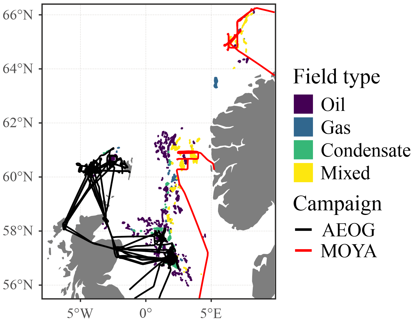
Figure 1AEOG (black) and MOYA (red) flight paths in the North and Norwegian seas. Coloured data points indicate the locations of different hydrocarbon field types (see Wilde et al., 2021, or Foulds et al., 2022, for detail). Note that the northernmost flight (∼65∘ N) took place over the Norwegian Sea and not the North Sea. However, for the purposes of simplicity here, all sample regions are referred to as the North Sea.
2.3 Identification of flared emissions and flaring efficiency calculations
Emissions from oil and gas facilities were identified in flight time-series data using the method described in Foulds et al. (2022). Briefly, plumes were both manually and statistically identified. Manual identification relied on visual inspection of the time-series data for enhancements. Statistical identification involved the determination of a background (and associated standard deviation) for each flight survey, manifested as a mode in the data of approximately 2 ppm CH4 (equivalent to the Northern Hemisphere CH4 background). Emission plumes were defined as enhancements that exceeded 2 standard deviations above the flight-specific background value. Manually and statistically identified plumes were compared to confirm likely emissions and not just singular, extreme data points in the time series. There is the potential that extremely small emission sources (with peak concentration enhancements within 2 standard deviations of the flight-specific background value) were not captured by this analysis. Such sources are indistinguishable from natural background variability and therefore cannot be accounted for.
Gas flaring could not be confirmed visually during the flight campaigns due to distance to targeted facilities. In the absence of visual flare confirmation, plumes associated with gas flaring were identified by correlated enhancements in the expected gas-phase components of flared hydrocarbon gas (i.e. CO2, CH4, C2H6, and NOx) above their respective background mole fractions. Plumes which did not contain correlated enhancements of all four of these components were discarded. For example, plumes containing enhancements in only CO2, CH4, and C2H6, and which therefore lacked enhancements in NOx, were discarded as they were assumed to result from gas venting without flaring. Similarly, plumes containing only enhancements in CO2 and NOx, and therefore lacking enhancements in either CH4 or C2H6, were assumed to result from emissions from power generation, such as diesel generators. Unfortunately, this approach does not preclude the possibility of including emissions from multiple mixed sources of CO2, CH4, C2H6, or NOx, such as co-located venting and power generation emissions.
Representative median-average background CO2, CH4, C2H6, and NOx mole fractions were determined for each plume using the 50 neighbouring 1 Hz measurements to either side of the plume. Plumes for which this was not possible due to missing background data for one or more components (i.e. fewer than 10 background data points) were discarded. Plumes were additionally discarded if one or more components lacked sufficient data within the plume (i.e. fewer than three data points). The NOx data generally suffered from data unavailability (see Table A1), with large proportions of missing 1 Hz data. During background measurement, missing data could be attributed largely to NOx mixing ratios below the instrument limit-of-detection (30 pptv), but missing data within plumes were also common. If enough data were present, missing NOx data were interpolated using normalised values of the CO2 and CH4 plume data. Figure 2 shows an example in which three missing data points within a single plume were interpolated and reconstructed using the mean-average normalised CO2 and CH4 data. Using this method relies on the assumption that each gas has an identical plume morphology, which may not always be the case if there are multiple co-located sources upwind (France et al., 2021). However, Fig. 2 clearly demonstrates that all four gas components showed consistent plume morphologies in this example. Finally, plumes were discarded if the maximum within-plume enhancement was within 2 standard deviations (2σ) of the local background mole fraction.
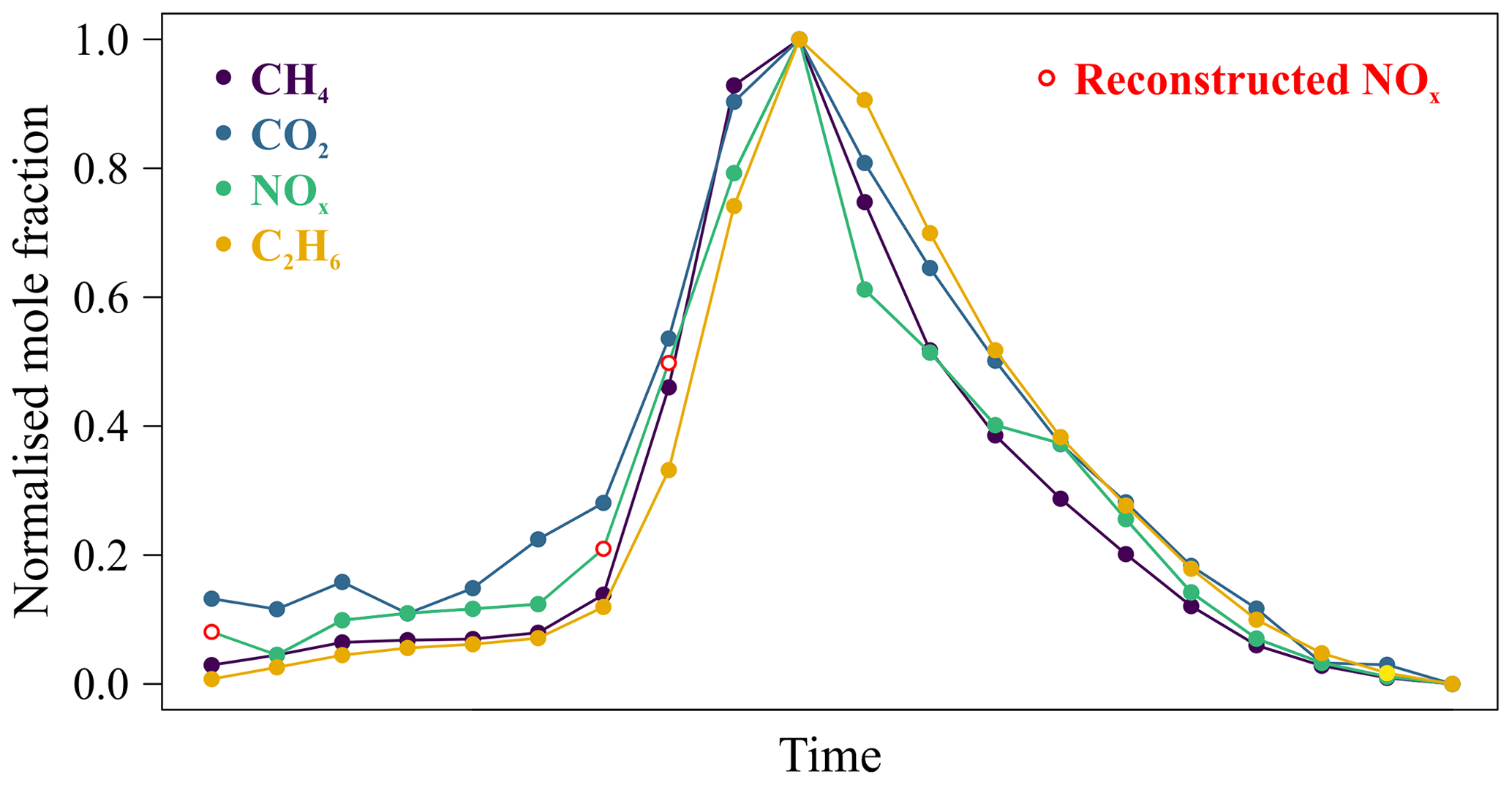
Figure 2Normalised mole fraction (enhancements above background) for a plume containing CO2, CH4, C2H6, and NOx. Three NOx data points were missing and were interpolated and reconstructed using the mean of normalised mole fractions of CO2 and CH4 (red data points).
Background mole fractions were subtracted from within-plume mole fractions to calculate enhancements. The resultant plume enhancements were then integrated (with respect to time) to determine the amount of each component within the emission plume. Integrating the data, rather than performing linear regression of co-located components, allows for slight temporal discrepancies in measured plumes to be ignored. Temporal discrepancies which lead to misaligned plumes could affect linear correlations between plume components.
2.3.1 Combustion efficiency calculations
Combustion efficiency (η) can be defined in multiple ways but is usually reported as the efficiency with which the gas flare converts hydrocarbons in the fuel gas into carbon dioxide (Eq. 1; Corbin and Johnson, 2014):
However, in many cases, the amount of carbon in the industrial fuel gas is unknown. Fuel composition can vary widely between production regions and within fields, as well as over the course of production. In cases where fuel composition is not known, combustion efficiencies have previously been approximated using the relationship between enhancements of CO2 and CH4 measured within the flare plume (Eq. 2; Nara et al., 2014):
ΔCO2 and ΔCH4 respectively refer to the enhancement of within-plume CO2 and CH4 above the local background mole fractions (see Sect. 2.3). The method presented in Eq. (2) assumes that all of the CO2 produced during gas flaring is due to combustion of CH4 i.e. no other hydrocarbons were combusted (the fuel gas is 100 % CH4) and that CO2 was not initially present in the fuel gas. This can lead to a slight overestimation of combustion efficiency if other hydrocarbons were present in the fuel gas and combusted. The extent of this overestimation depends on the exact composition of the fuel gas; the overestimation will be smaller the closer the proportion of CH4 is to the assumed value of 100 %.
As C2H6 mole fractions were also measured on board the FAAM aircraft, additional combustion efficiencies were calculated which account for the C2H6 enhancement within the plumes (Eq. 3). C2H6 oxidises to form two molar equivalents of CO2 and is therefore accounted for twice in Eq. (3):
where ΔC2H6 refers to the enhancement of within-plume C2H6 above the local background mole fraction. It should be noted that combustion efficiencies calculated with Eq. (3) will still overestimate the true combustion efficiency by some amount. Although CH4 and C2H6 typically dominate the fuel gas composition, other hydrocarbons are likely to be present (albeit, in small amounts) and cannot be accounted for here. However, this approach provides the best possible approximation in the absence of suitable instrumentation capable of resolving larger hydrocarbons at 1 Hz.
2.3.2 Destruction removal efficiency calculations
Destruction removal efficiency (DRE) is a measure of the efficiency with which a particular fuel gas component is oxidised within the flare (Eq. 4; Caulton et al., 2014; Corbin and Johnson, 2014):
where xi refers to any component of the fuel gas, Δxi is the enhancement above the background of that component within the plume, and Xi is the fractional composition of xi in the fuel gas. Equation (4) was used to calculate DREs for CH4 and C2H6.
Fuel gas composition values for various platforms were taken from privately communicated fuel composition data sourced via the Department for Business, Energy, and Industrial Strategy (BEIS). Where gas flare plumes could be satisfactorily attributed to single platforms (or groups of platforms), specific fuel composition values were used for Xi. In the absence of data for identified platforms, or where plumes could not be satisfactorily associated with specific platforms, the median fuel composition of all available data was used. The median fuel composition for CH4 was 0.845 and for C2H6 was 0.085. These fuel compositional values are consistent with those used in other works (e.g. Schwietzke et al., 2014; Sherwood et al., 2017). A Monte Carlo simulation (n=10 000) showed that calculated DREs were not sensitive to the choice of composition value, with a less than 1 % uncertainty (1σ) in mean DREs across the distribution of provided composition values.
2.3.3 Emission ratio calculations
NOx and C2H6 emission ratios (ERs) were calculated using CO2 and CH4 as the reference gas component:
ERs calculated in this way are also referred to as normalised excess mixing ratios (NEMRs) and assume that no chemical processing has occurred within the plume that could change the composition (Yokelson et al., 2013; Barker et al., 2020). This assumption is suitable for the components analysed here, as plumes were typically measured less than 10 km downwind of the source. The atmospheric lifetimes of CH4 (∼9 years; Turner et al., 2017) and C2H6 (∼2 months; Hodnebrog et al., 2018) ensure minimal chemical processing, and NOx is a conserved quantity unaffected by the conversion of NO to NO2 between emission and measurement.
2.4 Gas flaring emission inventories
Many emission inventories group emissions from the oil and gas sector into a single category, representing intentional venting, flaring, and leakage. The two emission inventories used here provide separate categories for flaring emissions.
The Global Fuel Exploitation Inventory (GFEI) is a globally gridded inventory of CH4 emissions from oil, gas, and coal exploitation, available at for 2019 (Scarpelli et al., 2020). The GFEI provides gridded emissions from different sectors (e.g. exploration, production, transport, transmission, and refining) and from specific processes such as venting and flaring, based on country reports submitted in accordance with the United Nations Framework Convention on Climate Change (UNFCCC). CH4 emissions from flaring during gas production, gas processing, and oil production were examined here. In the GFEI, CH4 emissions from flaring during oil exploration, gas exploration, and oil refining are grouped together with emissions from leakage and venting, and hence these emissions were not analysed. Comparisons between the GFEI and CH4 emission fluxes measured in the North Sea have already been made by Foulds et al. (2022) and Pühl et al. (2023).
The anthropogenic emission dataset Evaluating the Climate and Air Quality Impacts of Short-lived Pollutants (ECLIPSE) v5 provides global CH4 and NOx emissions (amongst other pollutants) for flaring as a separate sub-sector, at resolution for 2020 (Stohl et al., 2015). The ECLIPSE emission dataset was created using the Greenhouse gas - Air Pollution Interactions and Synergies (GAINS) model and international and national activity data for energy usage, industrial production, and agricultural activities. ECLIPSE products used GAINS emissions data up until 2010, after which emissions were projected into the future using current legislation and representative concentration pathways (Klimont et al., 2017).
Fifty-eight plumes from a maximum of 30 individual facilities were identified as containing emissions from gas flaring based on the criteria described in Sect. 2.3 (see Table A2 for numbers of excluded plumes). As some plumes from the same facility were sampled multiples times, there are two conceivable approaches to determining plume statistics. Firstly, measurements for plumes considered to originate from the same source could be combined, assuming that the combustion efficiency and emission ratios are constant. This would allow for uncertainty estimation, using the variability in the measured values. However, this may not be trivial as changing conditions (in e.g. wind direction) could mean that plumes do not always appear in the same location and therefore cannot always be positively attributed to the exact same source (in the absence of complex and time-consuming dispersion modelling). A second approach involves treating each intercepted plume as unique, by assuming that flaring conditions vary over time and that separate plume intercepts represent distinct measurements of instantaneous emissions. In this work, it was noted that plumes considered to have the same source origin (via approximate wind direction) had similar ΔC2H6:ΔCH4 emission ratios but that combustion efficiency varied with wind speed (see Appendix B). Hence, we have opted to treat the 58 identified plumes as individual and unique events. The following sections therefore present combustion efficiency, destruction removal efficiencies (for CH4 and C2H6), and emission ratio results for the 58 identified plumes.
Figure 3 illustrates the relative abundance of gaseous components in the 58 sampled flared plumes. As expected, CO2 was the largest component by at least an order of magnitude. The range in CH4, C2H6, and NOx spanned greater than 2 orders of magnitude. This could imply the measurement of emissions from flares of different operational characteristics and fuel gas volumes.
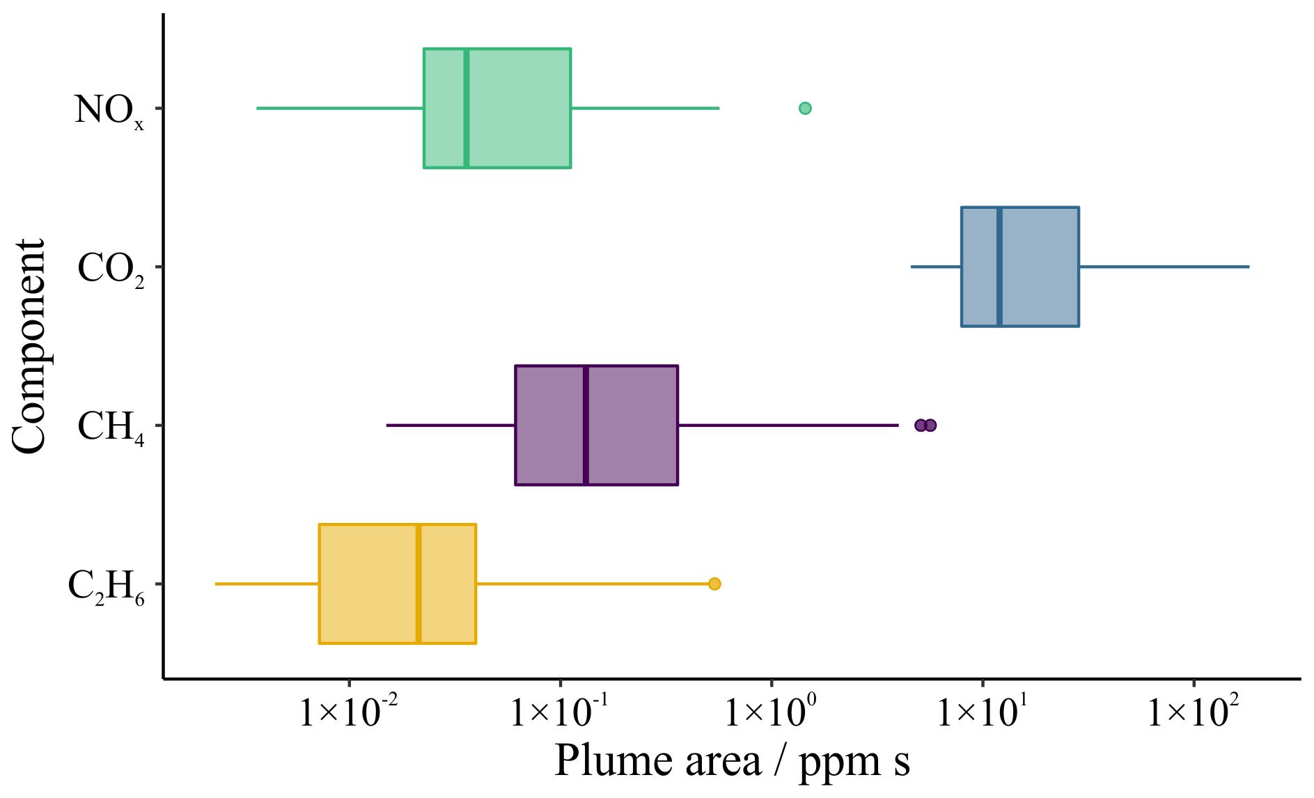
Figure 3Box and whisker distributions of integrated plume areas (in ppm s) above background for NOx, CO2, CH4, and C2H6 across the 58 identified flaring plumes. Box edges correspond to the first and third quartile (i.e. the 25th and 75th percentile) with the thicker, central line denoting the sample median (i.e. 50th percentile). The upper whisker extends to the greatest value no more than 1.5 multiples of the interquartile range (IQR) from the 75th percentile value. The lower whisker extends to the smallest value no less than 1.5 multiples of the IQR from the 25th percentile. Data beyond the extents of the whiskers were considered outlying points and were plotted individually (as circles). Note that the x axis has a logarithmic scale.
3.1 Combustion efficiency
Figure 4a shows the distribution of combustion efficiencies calculated without C2H6 (Eq. 2; Nara et al., 2014) and with C2H6 included (Eq. 3). Combustion efficiencies were marginally greater when C2H6 was not included in the calculation. However, even when including C2H6 in the calculation, efficiencies were high, with some plumes approaching 100 % efficiency and all efficiencies greater than 94 %. The median combustion efficiency across all sampled plumes without C2H6 included was 98.7 % (mean=98.3 % ± 1.4 %, 1σ), and the median efficiency with C2H6 included was 98.4 % (mean=97.9 % ± 1.7 %, 1σ) (see also Fig. C1). These values are exceptionally close to the 98 % combustion efficiency assumed by many emission inventories. However, Fig. 4a shows a strongly skewed distribution, indicating that assumptions of 98 % combustion efficiency is likely to be an overestimate in some cases. A summary of all results can be found in Table 1.
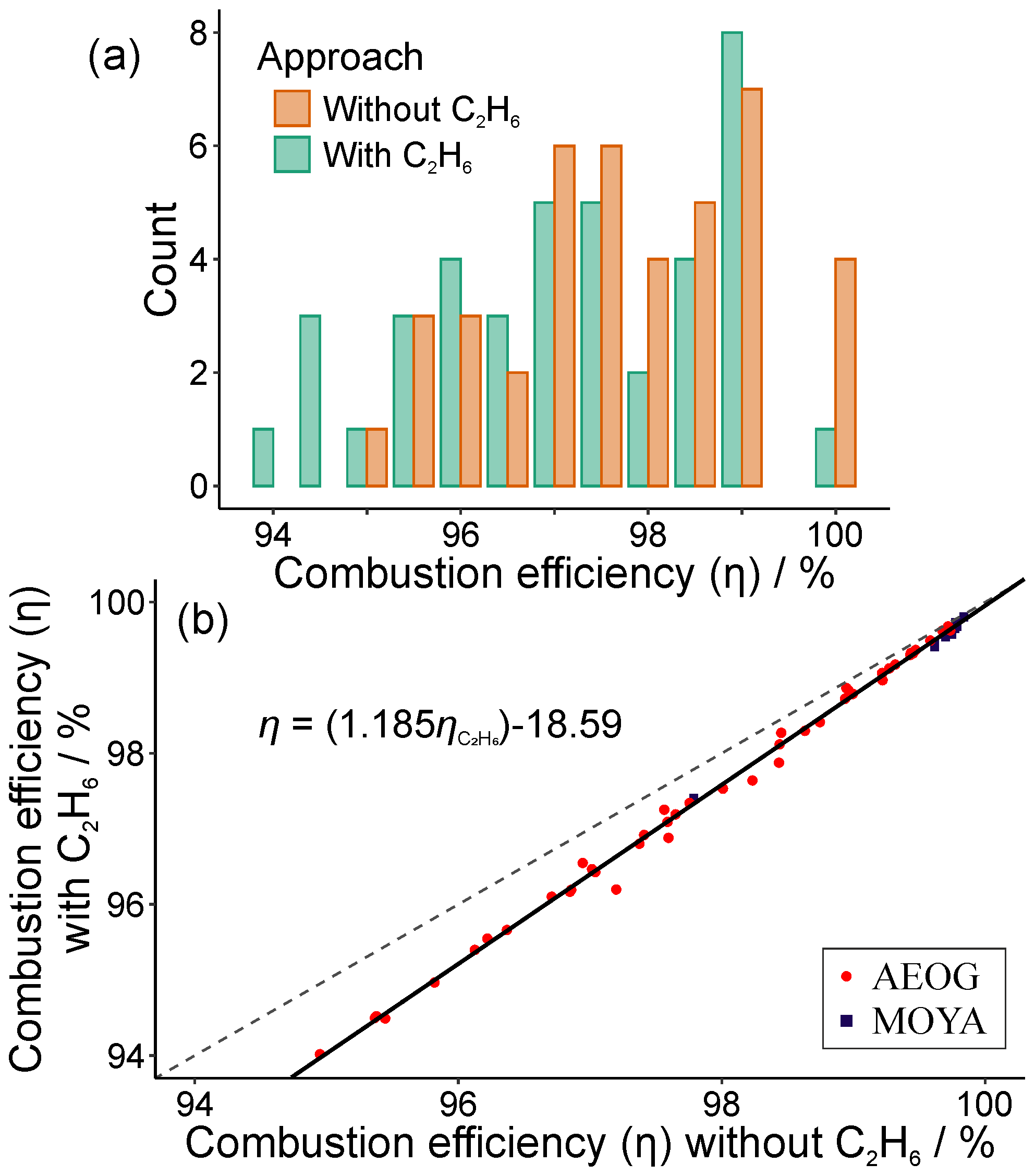
Figure 4(a) Histogram distribution of combustion efficiencies (η) calculated with C2H6 (green; Eq. 3) and without C2H6 (orange; Eq. 2). (b) Linear relationship between combustion efficiencies calculated with C2H6 and without C2H6. The solid black line shows the linear reduced major axis regression, with R2=0.996. The dashed black line shows a 1:1 ratio.
Table 1Summary of combustion efficiency, destruction removal efficiency (DRE), and emission ratio results.
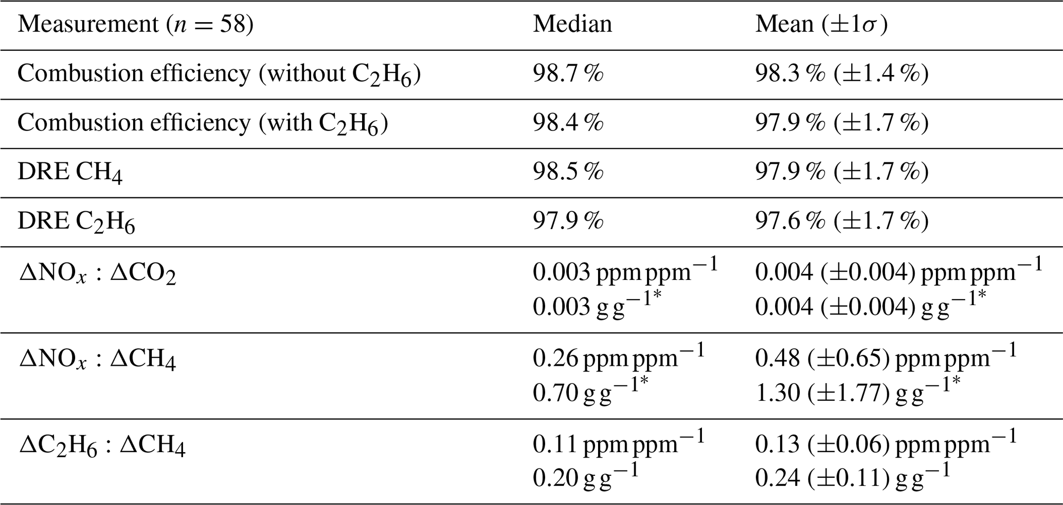
* Uses an average molar mass for NOx calculated using the average in-plume ratio of NO:NO2.
Figure 4b shows the linear relationship between combustion efficiencies calculated with and without C2H6. The linear relationship was estimated using reduced major axis regression. Combustion efficiencies calculated including C2H6 (Eq. 3) were marginally smaller than those calculated without C2H6 (Eq. 2). This relationship provides an approximation for estimating combustion efficiencies accounting for C2H6 in the absence of direct C2H6 observations. The R2 value for the linear regression was 0.996, indicating a high degree of model fit.
There was a small difference in combustion efficiencies (calculated including C2H6) measured during the AEOG and MOYA campaigns. The median combustion efficiency measured during AEOG (n=46 plumes) was 97.6 % (mean=97.5 % ± 1.6 %, 1σ), whilst the median combustion efficiency measured during MOYA (n=12) was 99.6 % (mean=99.4 % ± 0.6 %, 1σ). We cannot provide a conclusive explanation for this small difference in combustion efficiencies between the two campaigns but propose two explanations. AEOG sampled primarily UK-based platforms, whilst MOYA sampled Norwegian platforms. It may therefore be possible that differences in facility type, age, or operational practices in the two regions were responsible for the observed distinction in combustion efficiency. Alternatively, the measurements could be explained by differences in emissions from different hydrocarbon field types (see Fig. 1) with different gas compositions. Wilde et al. (2021) measured different VOC compositions in emissions from different field types in the North Sea region, and this may align with differences in the combustion efficiency observed here. However, Plant et al. (2022) found no correlation between combustion efficiency and factors such as well age, or gas-to-oil ratio, for onshore facilities in the USA.
Whilst combustion efficiency is expected to decrease with increasing wind speed (Jatale et al., 2016), recent studies have found little to no impact on flaring efficiency at wind speeds of up to 15 m s−1 (Caulton et al., 2014; Plant et al., 2022). Figure 5 shows an extremely weak but positive correlation (p=0.04; R2=0.08) between combustion efficiency and wind speed across the 58 identified plumes, although there was much scatter in the data. The observed trend was likely skewed by the greater number of plumes sampled under wind speeds of approximately 15 m s−1, several of which were measured during the MOYA campaign. Plumes sampled during the MOYA campaign had typically higher combustion efficiencies and therefore may be influencing the observed trend. The only plume measured in wind speeds of approximately 20 m s−1 (19.6 m s−1) showed a lower combustion efficiency (∼95.0 %) relative to many of those measured at wind speeds of 15 m s−1. Unfortunately, this was an isolated measurement, and a larger sample size of plumes sampled under higher wind speeds (>15 m s−1) would be required to draw meaningful conclusions on combustion efficiencies at such wind speeds. Our results were therefore in agreement with the conclusions of both Caulton et al. (2014) and Plant et al. (2022), which both showed no statistical relationship between combustion efficiency and wind speed.
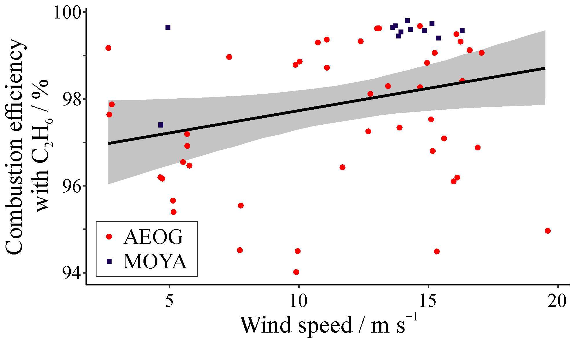
Figure 5Correlation between combustion efficiency (calculated including C2H6; Eq. 3) and wind speed (m s−1). The wind speed for each plume was calculated as the mean of 1 Hz wind speeds measured during and both 50 s before and after the plume. The black line shows an ordinary least squares linear regression of the data (p=0.04, R2=0.08), with the 95 % confidence interval shown in grey.
3.2 Destruction removal efficiencies (DREs)
Figure 6a shows the distribution of DREs calculated for both CH4 and C2H6 using Eq. (4) and fuel composition data provided by BEIS. The efficiency of CH4 destruction was marginally greater than that for C2H6, with median values of 98.5 % (mean=97.9 % ± 1.7 %, 1σ) and 97.9 % (mean=97.6 % ± 1.7 %, 1σ) for CH4 and C2H6 respectively (Table 1; see also Fig. C2). Gvakharia et al. (2017) reported marginally lower median DRE values of 97.1 % (±0.4 %) for CH4 and of 97.3 % (±0.3 %) for C2H6, from 37 flare plumes in the Bakken formation, United States. Plant et al. (2022) reported mean DRE values for CH4 of 97.3 %, 96.5 %, and 91.7 % from the Eagle Ford, Bakken, and Permian basins (United States) respectively. These results are in excellent agreement with our own. Figure 6b shows the relationship between DREs for the two fuel components, with a strong correlation between the two, even for DREs calculated for plumes from platforms for which flare gas composition was not available (see Sect. 2.3.2).
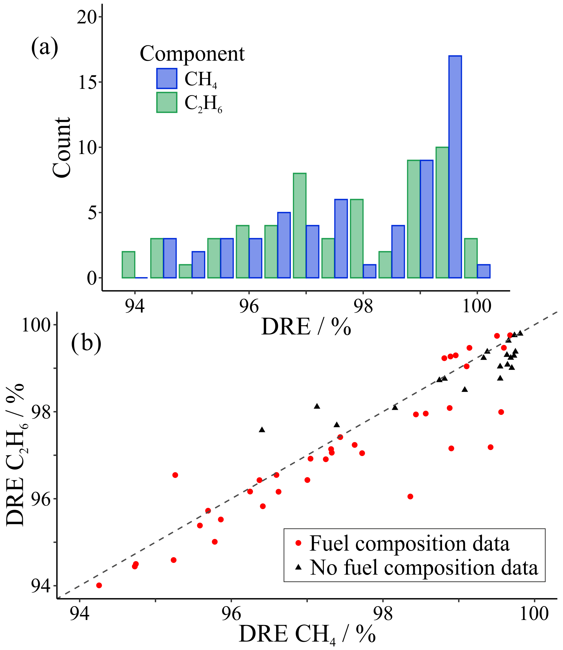
Figure 6(a) Histogram distribution of destruction removal efficiencies (DREs) calculated for CH4 (blue) and for C2H6 (green). (b) Comparison of DREs for CH4 and C2H6. The black dashed line shows a 1:1 ratio. The median fuel composition (CH4=0.845, C2H6=0.085) was used for plumes emitted from platforms for which no fuel composition data were available (black triangles).
3.3 Emission ratios
Figure 7 shows the distribution of NOx emission ratios calculated using both CO2 and CH4 as reference gases (ΔNOx:ΔCO2 and ΔNOx:ΔCH4 respectively). Mean NOx emission ratios were 0.004 ± 0.004 (1σ; median=0.003) ppm ppm−1 when using CO2 as the reference gas and 0.48 ± 0.65 (1σ; median=0.26) ppm ppm−1 when using CH4 as the reference gas (Table 1). There was substantial variability in the amount of NOx produced relative to both CO2 and CH4, as indicated by the large standard deviations about the mean ratios and the skewed long-tail distributions in both Fig. 7a and b. This may be a consequence of the inclusion of mixed emission sources within our dataset; it is difficult to distinguish between plumes containing pure flaring emissions and those potentially containing mixed emissions from co-located sources.
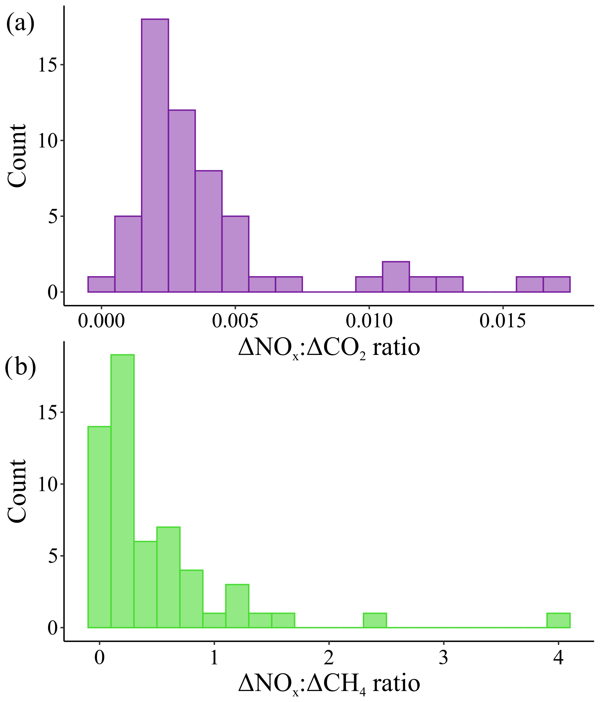
Figure 7Histogram distribution of NOx emission ratios (ppm ppm−1) (a) calculated using CO2 as the reference gas and (b) calculated using CH4 as the reference gas.
Four of the five greatest ΔNOx:ΔCH4 ratios (>1.1 ppm ppm−1) were measured over deep-water oilfields west of the Shetland Isles, where oil production is typically performed by floating production storage and offloading (FPSO) vessels. An additional high ΔNOx:ΔCH4 ratio (of 1.5 ppm ppm−1) was measured in a shallow water field, east of Scotland, also operated by an FPSO. FPSO vessels have been reported to contribute to 21 % of all offshore flaring volume (Charles and Davis, 2021), and the high ΔNOx:ΔCH4 ratios measured in the vicinity of their operation here could indicate a difference in operational practice (e.g. diesel generators on board FPSO vessels contributing to NOx emissions) compared with fixed platforms. The same five FPSO plumes also had the five greatest ΔNOx:ΔCO2 ratios.
Typically, NOx emissions from flares are estimated using emission factors and activity rates and often use flare heat as a proxy for NOx emission rates. Torres et al. (2012c) reported a mean NOx:CO2 ratio of 0.00020 (±0.00014) ppb ppb−1 from 24 test flares operated under a range of conditions (fuel gas composition, fuel gas flow, lower heating value, and steam or air assisted flow). In comparison, the smallest ΔNOx:ΔCO2 ratio measured in this study was 0.0005 ppb ppb−1. The reason for the order of magnitude difference between the NOx:CO2 ratios measured in this work and those reported by Torres et al. (2012c) is unknown but is perhaps due to the specific flaring conditions measured in each case (Torres et al. measured emissions from manual test flares with targeted gas compositions and heating values and not real-world flares operating in the North Sea).
Figure 8a shows the relationships between combustion efficiency (calculated with C2H6) and ΔNOx:ΔCH4. Higher combustion efficiencies were typically associated with higher relative amounts of NOx, consistent with higher temperature flaring. Figure 8a appears to show an exponential relationship between combustion efficiency and ΔNOx:ΔCH4, but a linear regression is also shown for comparison (; R2=0.24). NOx only appeared to be produced in substantial amounts (relative to CH4) at combustion efficiencies greater than ∼96 %, with a general increase in NOx ratios with increasing combustion efficiency beyond this point. However, plumes measured during the MOYA campaign appeared to have reduced NOx ratios relative to many of those measured in AEOG, despite having greater combustion efficiencies, implying possible differences in flare operation. Torres et al. (2012c) found a similar result, with minimal NOx produced below a combustion efficiency threshold of roughly 80 %, above which NOx production increased roughly linearly. Wind speed appeared to have very little influence on NOx emission ratios (p=0.2; R2=0.03) (Fig. 8b).
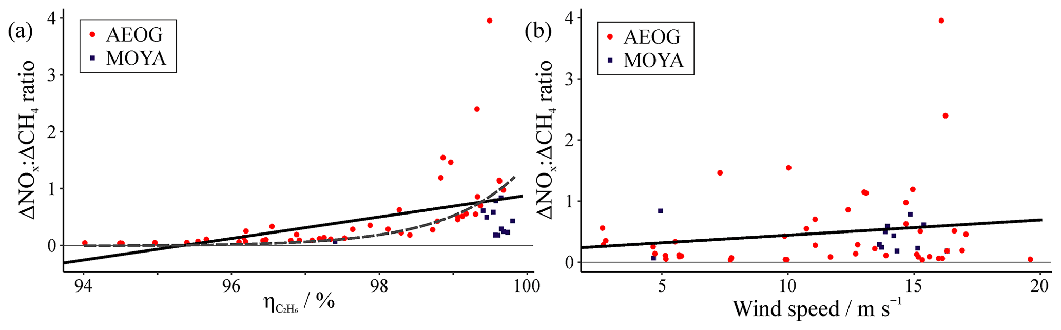
Figure 8Correlation between measured ΔNOx:ΔCH4 ratio and (a) combustion efficiency calculated with C2H6 () and (b) wind speed. Solid black lines show ordinary least squares linear regressions with and 0.2, as well as R2=0.24 and 0.03, for the relationship with combustion efficiency and wind speed respectively. Dashed black line shows the exponential relationship (y=ex) between ΔNOx:ΔCH4 and combustion efficiency, for comparison.
The mean ΔC2H6:ΔCH4 ratio across all gas flaring plumes was 0.13 ± 0.06 (1σ) ppm ppm−1, with ratios ranging between 0.04 and 0.33 (median=0.11) ppm ppm−1 (Table 1 and Fig. C3). These results were in excellent agreement with measurements reported by Wilde et al. (2021), in which ΔC2H6:ΔCH4 ratios ranged between 0.03 and 0.18 ppm ppm−1. Ratios of between 0.03 and 0.08 ppm ppm−1 were also measured for oil and gas emissions in the southern North Sea (Pühl et al., 2023). It should be noted that the ratios measured by Wilde et al. (2021) and Pühl et al. (2023) were not specifically attributed to flared emissions and were likely to be representative of total emissions from oil and gas infrastructure, including any vented emissions or fugitive natural gas leaks. Their ratios therefore cannot be compared directly against our own results but may serve as an indication of the relative impacts of flaring on ΔC2H6:ΔCH4 ratios. ΔC2H6:ΔCH4 ratios greater than 0.1 ppm ppm−1 are typically associated with emissions from oil wells, whilst ratios below 0.1 ppm ppm−1 are usually associated with emissions from gas wells (Xiao et al., 2008; Wilde, 2021).
3.4 Emission inventories
The ECLIPSE inventory contains flaring emission products for both CH4 and NOx, and hence the NOx:CH4 ratio for this dataset was calculated. Figure 9 shows the ECLIPSE NOx:CH4 emission ratio in the North Sea (for flared emissions), in units of mass per unit mass. Conversion of the ΔNOx:ΔCH4 ratio measured in this work (in units of mole fraction per unit mole fraction) yields a median ΔNOx:ΔCH4 of 0.70 g g−1 (mean=1.30 (±1.77) g g−1). The measured values were roughly 30 times greater than the highest ECLIPSE ratios in the North Sea, although NOx:CH4 ratios in the ECLIPSE inventory globally reached values greater than 2.0 Gg Gg−1. Our study finds that the ECLIPSE inventory may underestimate the NOx:CH4 ratio by more than an order of magnitude in the North Sea region.
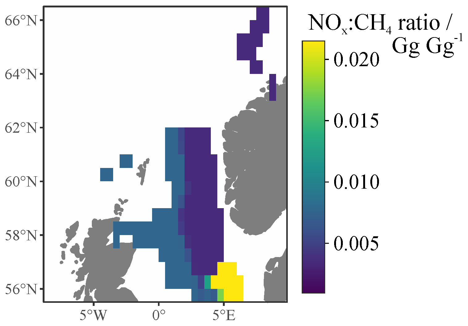
Figure 9ECLIPSE v5 flaring NOx:CH4 ratios in the North Sea.
There are a few possible reasons for this disparity in NOx:CH4 ratios between datasets. Firstly, inventories are typically representative of annual emissions, whereas our ratios are snapshots calculated for emissions at the time of sampling. If flaring emissions can be expected to vary throughout the year, either as a result of changes to operation or to local meteorology, this may lead to differences. Secondly, our measurements are only comparable to inventory grid cells if a representative population of flaring emissions were sampled. Thirdly, the ECLIPSE inventory for 2020 was calculated by projecting activity data for 2010 forwards in time using legislative and representative concentration pathways (Klimont et al., 2017), and these may not be valid for current emission scenarios.
Flaring in the UK North Sea reportedly fell by 23 % in 2020 relative to 2019, but ∼740 million cubic metres (7.4×10⁸ m3) of natural gas were still reported to have been flared (OGA, 2021). Here, we use the median gas composition of flared gas provided by BEIS for this region (CH4=0.845, and C2H6=0.085) and the median DREs for CH4 and C2H6 (calculated in Sect. 3.2) to estimate total emissions of CO2, CH4, and C2H6 from North Sea flaring. We estimate that flaring in the UK North Sea resulted in total emissions of 1.4 Tg yr−1 CO2, 6.3 Gg yr−1 CH4, and 1.7 Gg yr−1 C2H6. Using the calculated CH4 emission total here and the median ΔNOx:ΔCH4 ratio derived in Sect. 3.3, we estimate total emissions of 3.9 Gg yr−1 NOx from flaring in the North Sea region. These values, estimated using reported flaring volumes and statistics measured as part of this work, can be compared against the total emissions estimated by inventories for the North Sea region. ECLIPSE reports 30 times greater emissions of CH4 from the North Sea, with 177 Gg yr−1 CH4, but smaller emissions of NOx of 0.9 Gg yr−1 NOx. The lower NOx estimate is potentially the result of the lower NOx:CH4 ratio in the ECLIPSE model, which largely underestimated the NOx:CH4 ratio relative to that measured in this work (Sect. 3.4). Alternatively, the Global Fuel Exploitation Inventory (GFEI) provides CH4 emissions of 13.9 Gg yr−1 CH4, 3 times greater than our own estimate here for the North Sea region. The GFEI total can be broken down into 11.8 Gg yr−1 CH4 (85 %) from flaring during oil exploitation, 1.5 Gg yr−1 CH4 (11 %) from gas processing, and 0.5 Gg yr−1 CH4 (4 %) from gas production. The large difference in ECLIPSE estimated CH4 flaring emissions could be a result of the inventory being a projected emission scenario for 2020, based on emissions representative of 2010 and legislation pathways (Klimont et al., 2017). Neither inventory provided flaring emission products for CO2 or C2H6, and GFEI did not include NOx flaring emissions. These results are summarised in Table 2.
Table 2Estimated total emissions of CO2, CH4, C2H6, and NOx from flared natural gas in the North Sea (in Gg) and globally (in Tg).

∗ Uses the DRE measured in this work for offshore flaring (25 % of global total; IEA, 2018) and the DRE measured by Plant et al. (2022) for onshore flaring (75 % of global total; IEA, 2018). 1 Stohl et al. (2015). 2 Scarpelli et al. (2020). 3 IEA (2021).
Extrapolating the results of this work to the global scale relies on the crude assumption that global natural gas supplies are analogous to those found in the North Sea and that operational practices are consistent across all fields and regions both onshore and offshore. In practice, flaring operations in the North Sea have some of the most stringent management systems due to a proactive regulatory regime. Such an extrapolation could be useful even with these substantial assumptions, as measurements of combustion efficiencies and NOx emission ratios from flared gas are exceptionally rare, especially offshore. Using the effective DRE for onshore flaring (of 91.1 %) measured by Plant et al. (2022) (which includes additional estimates of emissions from unlit flares), a total globally extrapolated emission of 7.6 Tg CH4 from all onshore and offshore flaring can be estimated. The proportion of unlit flares was observed to be between 3 % and 5 % of all flares across different onshore basins in the United States (Lyon et al., 2021; Plant et al., 2022) and therefore may be significant for extrapolating total emissions. If we assume the DRE value measured by Plant et al. (2022) is appropriate for all onshore production and that our own measured DRE values are appropriate for offshore production, we can provide an alternative global extrapolation that accounts for any systematic differences between onshore and offshore flaring.
Approximately 25 % of global oil and gas supplies are produced offshore (IEA, 2018). The IEA reported that 142 billion cubic metres (142×109 m3) of natural gas were flared worldwide in 2020 (IEA, 2021). If flaring is practiced to the same extent both onshore and offshore, then it follows that offshore flaring was responsible for approximately 36×109 m3 of the global total. By assuming that the median DREs calculated here and the median fuel gas composition values provided by BEIS for North Sea platforms are appropriate for offshore production globally, we estimate global offshore flaring emissions of 65 Tg yr−1 CO2, 0.3 Tg yr−1 CH4 and 0.08 Tg yr−1 C2H6. Using the onshore measured effective DRE for CH4 from Plant et al. (2022) for both CH4 and C2H6, we estimate global onshore flaring emissions of 180 Tg yr−1 CO2, 5.3 Tg yr−1 CH4, and 1.0 Tg yr−1 C2H6. Total global emissions, from both onshore and offshore flaring, were therefore 245 Tg yr−1 CO2, 5.6 Tg yr−1 CH4, and 1.1 Tg yr−1 C2H6. Our estimate of CO2 emissions is consistent with the IEA estimate, but our estimate of CH4 emission is lower. This is due to the higher combustion efficiency measured for the North Sea (median=98.4 %) and used for offshore estimates, compared to the lower estimate of 92 % used by the IEA for both onshore and offshore flaring globally. Using the median ΔNOx:ΔCH4 ratio, flaring was estimated to be responsible for emissions of 3.6 Tg yr−1 NOx globally. Comparing to the emission inventories, ECLIPSE provides much greater total annual emissions of CH4, of 109 Tg yr−1, but lower emissions of NOx, of 236 Gg yr−1. GFEI provides total global CH4 emissions of 630 Gg yr−1, of which oil exploitation contributes 500 Gg yr−1 (79 %), gas processing 95 Gg yr−1 (15 %), and gas production 35 Gg yr−1 (6 %). The nature of the ECLIPSE inventory estimates for 2020 (projected emissions based on 2010 emissions and legislation pathways) means that some major emission sources are missed. For example, no flaring emissions were prescribed to the Bakken formation region in the northern United States, despite recent (post-2010) large-scale developments in shale gas there. Total global emissions of CO2, CH4, C2H6, and NOx are summarised in Table 2.
Fifty-eight plumes were identified as containing emissions likely to result from flaring of natural gas from offshore oil and gas facilities in the North Sea. Combustion efficiency, the efficiency with which the flares convert carbon in the fuel gas into CO2, was calculated for each of these plumes using two approaches, with and without accounting for C2H6 in the flare plume. The median combustion efficiency, of 98.4 % (with C2H6) and 98.7 % (without C2H6), was in agreement with the assumed value of 98 % used by many emission inventories for flaring combustion efficiency. The linear relationship between combustion efficiencies calculated with and without C2H6 could be used to derive more accurate combustion efficiencies in the absence of measurements of C2H6, assuming similar fuel gas composition. Destruction removal efficiencies (DREs) were also calculated for CH4 and C2H6 in each plume, making use of fuel gas compositions provided by BEIS. Median DRE values were 98.5 % and 97.9 % for CH4 and C2H6 respectively.
NOx emission ratios were calculated using both CO2 and CH4 as reference gases, with median values of 0.003 and 0.26 ppm ppm−1 for CO2 and CH4 as a reference respectively. All five of the greatest ΔNOx:ΔCH4 ratios (>1.1 ppm ppm−1) and ΔNOx:ΔCO2 ratios (> 0.011 ppm ppm−1) were measured in the vicinity of floating production storage and offloading vessels, which may indicate a difference in their flaring operation compared with fixed platforms. C2H6 emission ratios were calculated using CH4 as a reference gas. The median value for ΔC2H6:ΔCH4, of 0.11, was in excellent agreement with C2H6 emission ratios calculated for similar datasets. Wind speed appeared to have only a small impact on both the combustion efficiency of the flares and the relative amount of NOx produced, although more data on flares operating in wind speeds of greater than 15 m s−1 are needed.
Total North Sea and total global emissions due to flaring were estimated using reported gas flaring volumes and the statistics calculated in this work. For the North Sea, emissions were estimated as 1.4 Tg yr−1 CO2, 6.3 Gg yr−1 CH4, 1.7 Gg yr−1 C2H6, and 3.9 Gg yr−1 NOx, whilst globally emissions were extrapolated to 245 Tg yr−1 CO2, 5.6 Tg yr−1 CH4, 1.1 Tg yr−1 C2H6, and 3.6 Tg yr−1 NOx. Although many emission inventories do include emissions from flaring, most do not provide separate values for this source and instead aggregate emissions due to flaring with other oil and gas sector emissions. This makes comparison challenging. However, we find that the ECLIPSE inventory overestimates CH4 emissions from flaring by a factor of 30 in the North Sea but underestimates NOx emissions by a factor of 4. The GFEI product overestimates CH4 emissions from flaring by a factor of 2 in the North Sea.
The skewed distribution of combustion efficiencies found in this, and other, studies indicates that many flares operate below the assumed standard efficiency for combustion. Inefficient combustion, together with the prevalence of unlit flares which directly vent CH4 to the atmosphere, contribute to large CH4 emissions. Hence, improving natural gas disposal and flaring practices represents a viable strategy for mitigating carbon emissions from the oil and gas sector.
Table A1Data availability (percentage of total 1 Hz data) for CO2, CH4, C2H6, and NOx during FAAM AEOG and MOYA flights. Data availability below 50 % are given in italics. It should be noted that 100 % data availability would not be expected for various reasons. Firstly, data files might contain data outside of when the instruments were operational (e.g. before take-off or after landing) which were removed for analysis, and secondly, due to the presence of instrument calibrations, for which data were flagged and removed.
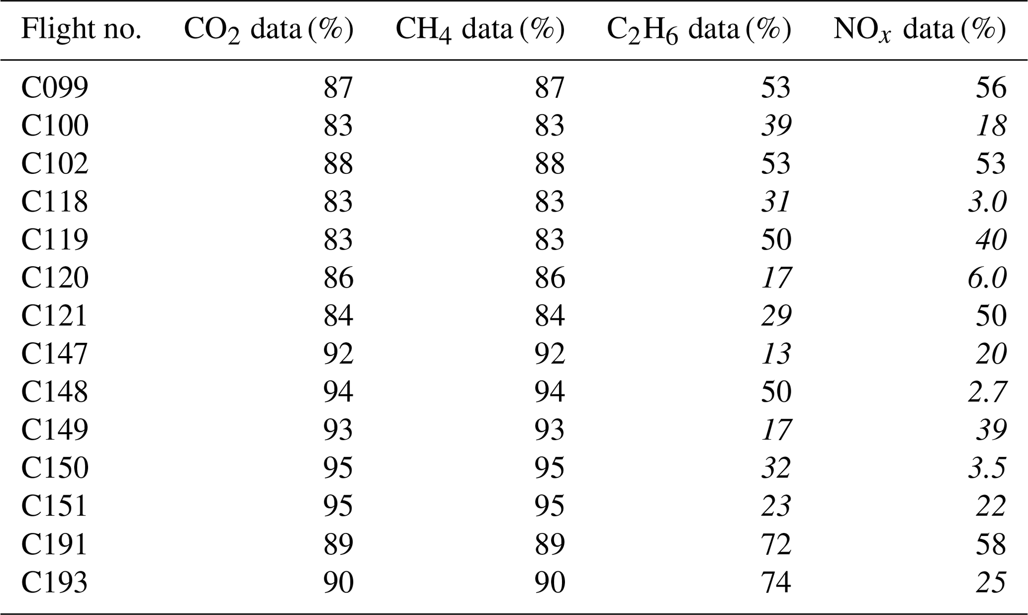
Table A2Reasons for plume exclusion. See Sect. 2.3 for detailed criteria descriptions. Note that plumes could be excluded based on failing multiple criteria.
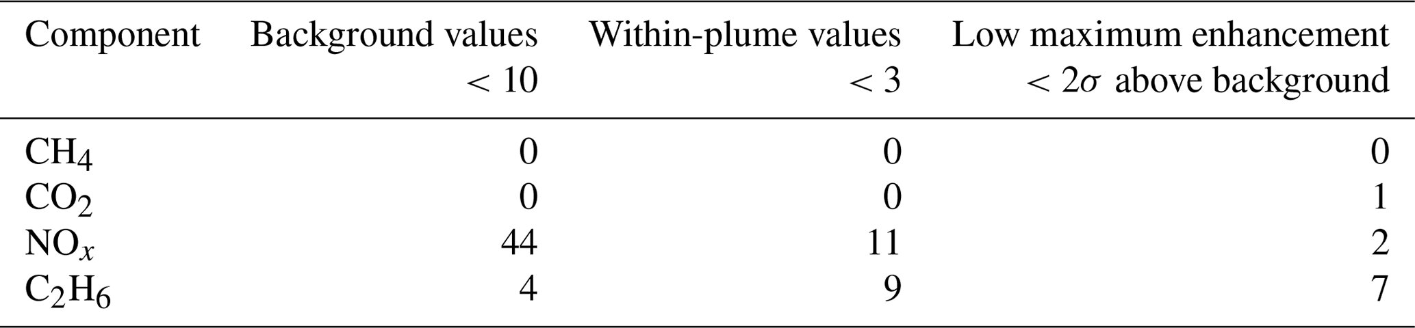

Figure B1CH4 mole fraction (see colour scale) measurements in the North Sea on 4 March 2019. Black arrows show the 60 s mean wind direction. Two distinct emission plumes (containing enhancements in CH4, as well as CO2, NOx, and C2H6) are shown, labelled Plume A and Plume B. Note that some of these peaks were removed from analysis due to a lack of measured data (primarily NOx) either within the plume or within the background (see Appendix A).
Table B1Combustion efficiencies (with and without C2H6) and emission ratios for peaks within two plumes sampled on 4 March 2019 (see Fig. B1).
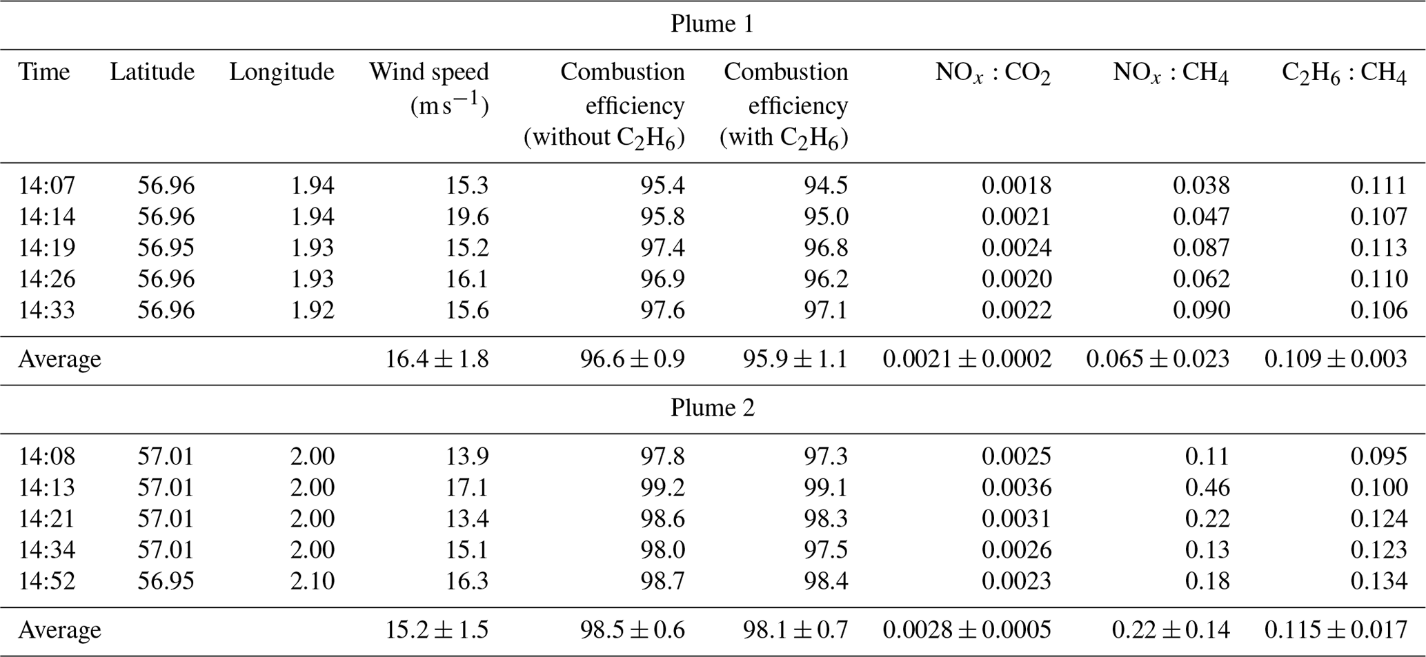
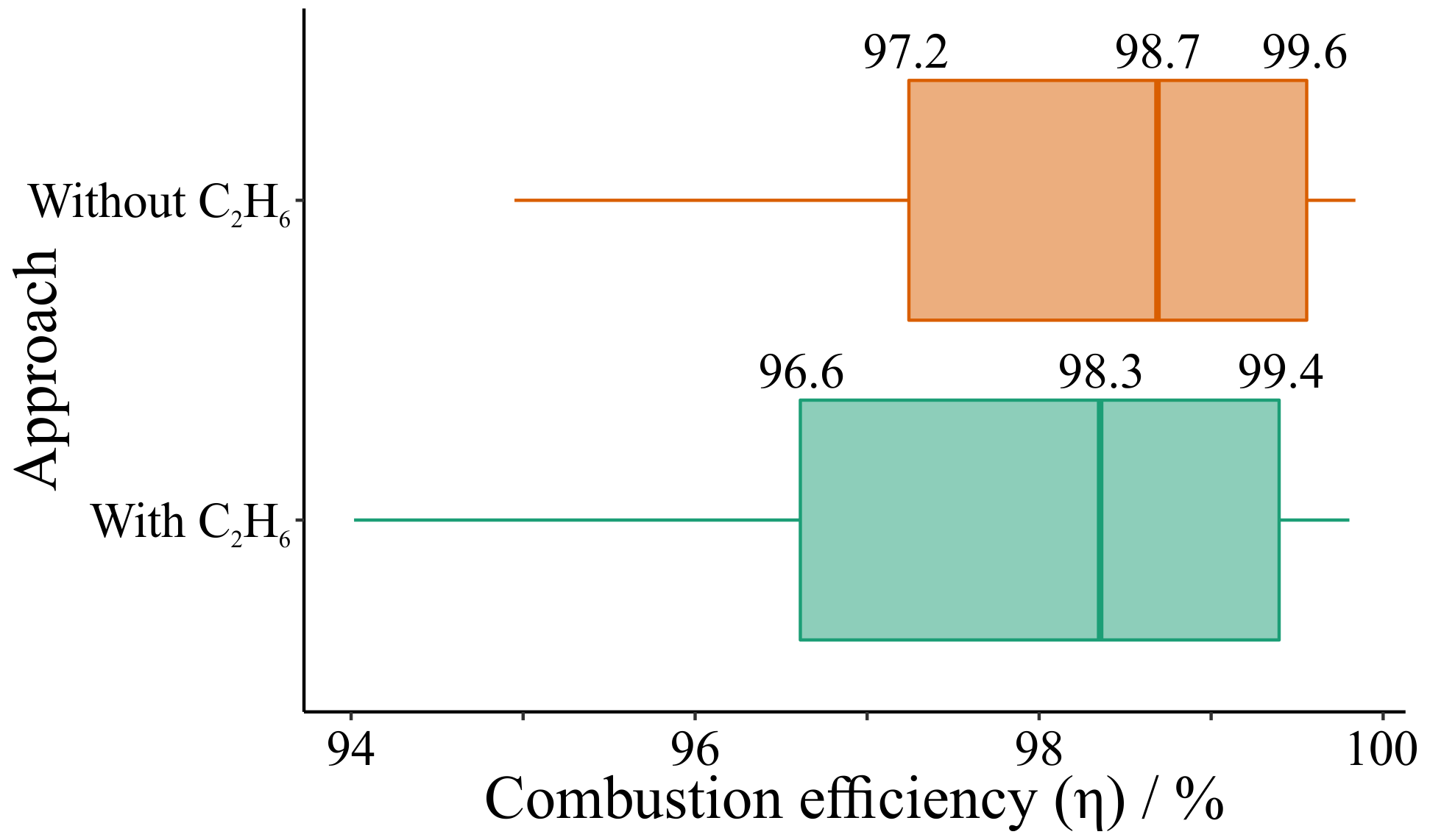
Figure C1Box and whisker plots of combustion efficiencies calculated without C2H6 (Eq. 2; orange, top row) and with C2H6 (Eq. 3; green, bottom row).

Figure C2Box and whisker plots of destruction removal efficiencies (DREs) for CH4 (blue; top row) and C2H6 (green; bottom row).
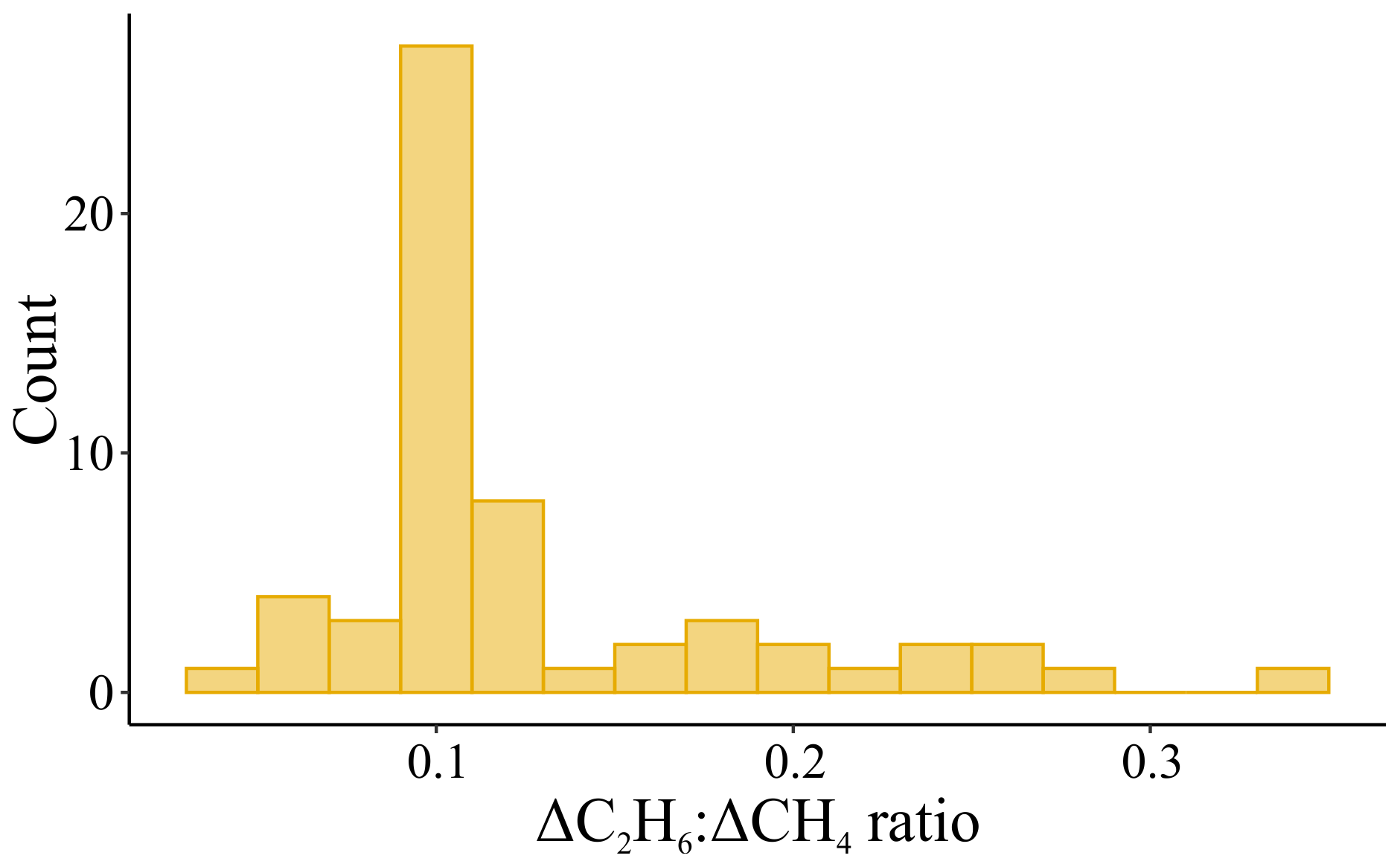
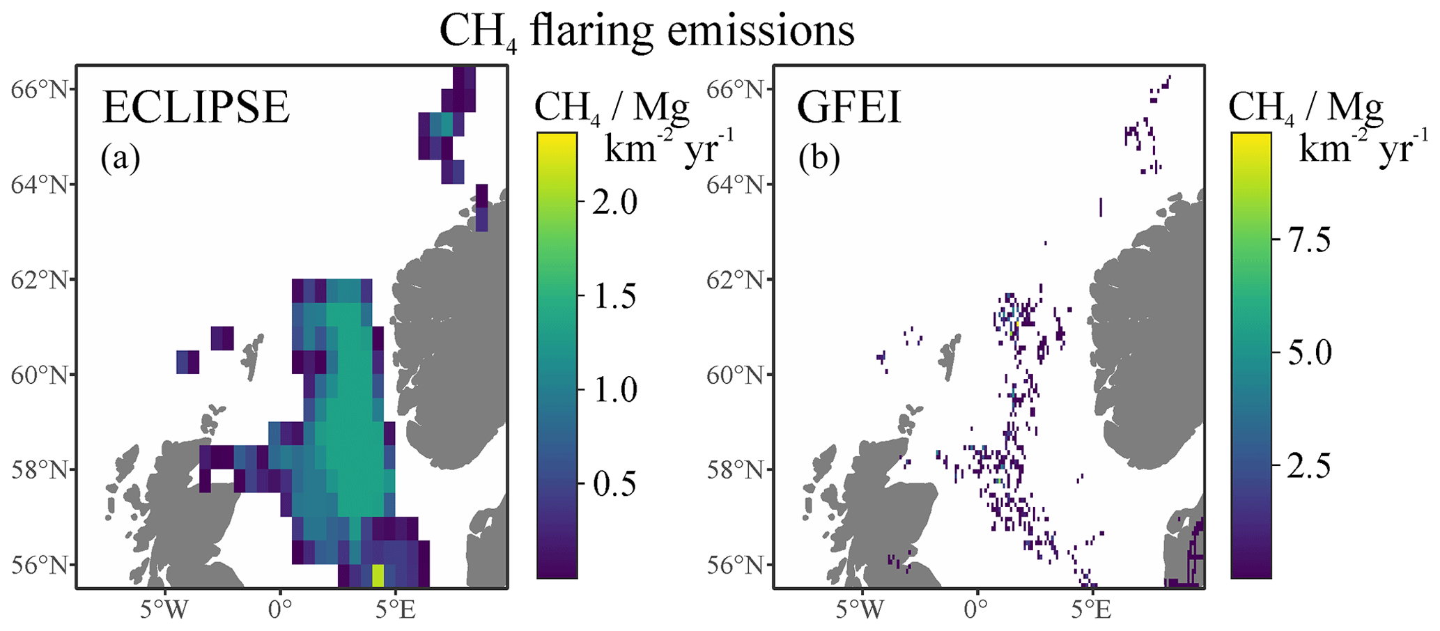
Figure D1(a) ECLIPSE v5 CH4 flaring emissions over the North Sea, at for 2020 (Stohl et al., 2015). (b) GFEI CH4 flaring emissions over the North Sea, at for 2019 (Scarpelli et al., 2020).

Figure D2ECLIPSE v5 NOx flaring emissions over the North Sea, at for 2020 (Stohl et al., 2015).
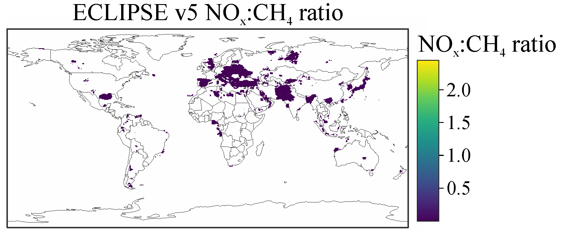
Figure D3ECLIPSE v5 NOx:CH4 ratio, at for 2020 (Stohl et al., 2015).
Data from the AEOG and MOYA FAAM aircraft campaigns are available from the Centre for Environmental Data Analysis (CEDA) archive at https://catalogue.ceda.ac.uk/uuid/c94601501623483aa0a12e29ce99c0e0 (Crosier, 2022) and https://catalogue.ceda.ac.uk/uuid/dd2b03d085c5494a8cbfc6b4b99ca702 (Nisbet, 2022) respectively. Please note that access to CEDA data sets and resources requires a free CEDA login account. This is in line with funder policy and ensures appropriate use and citation of public data. GFEI emission grids are available for download from the Harvard Dataverse at https://doi.org/10.7910/DVN/HH4EUM (Scarpelli and Jacob, 2021). ECLIPSE v5a global emission grids based on the GAINS model are publicly available from https://previous.iiasa.ac.at/web/home/research/researchPrograms/air/ECLIPSEv5a.html (IIASA, 2015).
JTS: formal analysis, methodology, visualisation, and writing – original draft preparation; AF: formal analysis, methodology, and writing – original draft preparation; SW: formal analysis, investigation, visualisation, and writing – original draft preparation; PB: data curation and investigation; FS: data curation and investigation; JL: conceptualisation, investigation, project administration, and funding acquisition; RP: conceptualisation, investigation, and funding acquisition; RB: investigation and funding acquisition; IC: investigation; SM: investigation and funding acquisition; SC: data curation and investigation; SJBB: data curation and investigation; SY: data curation and investigation; StS: writing – original draft preparation; GA: conceptualisation, investigation, methodology, project administration, writing – original draft preparation, and funding acquisition.
The contact author has declared that none of the authors has any competing interests.
Publisher's note: Copernicus Publications remains neutral with regard to jurisdictional claims in published maps and institutional affiliations.
We would like to thank Airtask Ltd. (who flew the aircraft) and all those involved in the operation and maintenance of the BAe-146-301 Atmospheric Research Aircraft, including FAAM, Avalon Aero, UK Research and Innovation (UKRI), and the University of Leeds. We also acknowledge the Offshore Petroleum Regulator for Environment and Decommissioning (OPRED) and Ricardo Energy & Environment for their involvement as project partners on the AEOG project. Any opinions, findings, conclusions, or recommendations expressed in this material are those of the author(s) and do not necessarily reflect the views of their respective institutions.
This work was supported by the Climate and Clean Air Coalition (CCAC) Oil and Gas Methane Science Studies (MSS) hosted by the United Nations Environment Programme. Funding was provided by the Environmental Defense Fund, the Oil and Gas Climate Initiative, the European Commission, and the CCAC (grant no. DTIE19-020). The aircraft data used in this publication were collected as part of two projects: the Demonstration Of A Comprehensive Approach To Monitoring Emissions From Oil and Gas Installations (AEOG) project (grant no. NE/R01451X/1) and the Methane Observations and Yearly Assessment (MOYA) project (grant no. NE/N015835/1), both funded by the Natural Environment Research Council (NERC).
This paper was edited by Eduardo Landulfo and reviewed by two anonymous referees.
Allen, D. T., Smith, D., Torres, V. M., and Saldaña, F. C.: Carbon dioxide, methane and black carbon emissions from upstream oil and gas flaring in the United States, Curr. Opin. Chem. Eng., 13, 119–123, https://doi.org/10.1016/j.coche.2016.08.014, 2016.
Anejionu, O. C. D., Whyatt, J. D., Blackburn, G. A., and Price, C. S.: Contributions of gas flaring to a global air pollution hotspot: Spatial and temporal variations, impacts and alleviation, Atmos. Environ., 118, 184–193, https://doi.org/10.1016/j.atmosenv.2015.08.006, 2015.
Barker, P. A., Allen, G., Gallagher, M., Pitt, J. R., Fisher, R. E., Bannan, T., Nisbet, E. G., Bauguitte, S. J.-B., Pasternak, D., Cliff, S., Schimpf, M. B., Mehra, A., Bower, K. N., Lee, J. D., Coe, H., and Percival, C. J.: Airborne measurements of fire emission factors for African biomass burning sampled during the MOYA campaign, Atmos. Chem. Phys., 20, 15443–15459, https://doi.org/10.5194/acp-20-15443-2020, 2020.
Cain, M., Warwick, N. J., Fisher, R. E., Lowry, D., Lanoisellé, M., Nisbet, E. G., France, J., Pitt, J., O'Shea, S., Bower, K. N., Allen, G., Illingworth, S., Manning, A. J., Bauguitte, S., Pisso, I., and Pyle, J. A.: A cautionary tale: A study of a methane enhancement over the North Sea, J. Geophys. Res.-Atmos., 122, 7630–7645, https://doi.org/10.1002/2017JD026626, 2017.
Charles, J.-H. and Davis, M.: Flaring at FPSOs: Out of sight, but not out of mind, Capterio, https://capterio.com/wp-content/uploads/2021/02/20210101-Flaring-at-FPSOs-out-of- sight-but-not-out-of-mind.pdf (last access: June 2022), 2021.
Caulton, D. R., Shepson, P. B., Cambaliza, M. O. L., McCabe, D., Baum, E., and Stirm, B. H.: Methane destruction efficiency of natural gas flares associated with shale formation wells, Environ. Sci. Technol., 48, 9548–9554, https://doi.org/10.1021/es500511w, 2014.
Corbin, D. J. and Johnson, M. R.: Detailed expressions and methodologies for measuring flare combustion efficiency, species emission rates, and associated uncertainties, Ind. Eng. Chem. Res., 53, 19359–19369, https://doi.org/10.1021/ie502914k, 2014.
Crosier, J.: FAAM AEOG: Demonstration of comprehensive approach to monitoring atmospheric emissions from oil and gas installations, National Centre for Atmospheric Science (NCAS), CEDA Archive [data set], https://catalogue.ceda.ac.uk/uuid/c94601501623483aa0a12e29ce99c0e0 (last access: June 2022), 2022.
Dlugokencky, E. J., Myers, R. C., Lang, P. M., Masarie, K. A., Crotwell, A. M., Thoning, K. W., Hall, B. D., Elkins, J. W., and Steele, L. P.: Conversion of NOAA atmospheric dry air CH4 mole fractions to a gravimetrically prepared standard scale, J. Geophys. Res.-Atmos., 110, D18306, https://doi.org/10.1029/2005JD006035, 2005.
Elvidge C. D., Bazilian, M. D., Zhizhin, M., Ghosh, T., Baugh, K., and Hsu, F.-C.: The potential role of natural gas flaring in meeting greenhouse gas mitigation targets, Energy Strateg. Rev., 20, 156–162, https://doi.org/10.1016/j.esr.2017.12.012, 2018.
Eman, E. A.: Gas flaring in industry: An overview, Petrol. Coal, 57, 532–555, 2015.
EPA, AP-42: Fifth Edition Compilation of Air Emissions Factors, Vol. 1: Stationary Point and Area Sources, Chap. 13.5: Industrial Flares, https://www.epa.gov/sites/default/files/2020-10/documents/13.5_industrial_flares.pdf (last access: August 2022), 2018.
Fawole, O. G., Cai, X.-M., and MacKenzie, A. R.: Gas flaring and resultant air pollution: A review focusing on black carbon, Environ. Pollut., 216, 182–197, https://doi.org/10.1016/j.envpol.2016.05.075, 2016.
France, J. L., Bateson, P., Dominutti, P., Allen, G., Andrews, S., Bauguitte, S., Coleman, M., Lachlan-Cope, T., Fisher, R. E., Huang, L., Jones, A. E., Lee, J., Lowry, D., Pitt, J., Purvis, R., Pyle, J., Shaw, J., Warwick, N., Weiss, A., Wilde, S., Witherstone, J., and Young, S.: Facility level measurement of offshore oil and gas installations from a medium-sized airborne platform: method development for quantification and source identification of methane emissions, Atmos. Meas. Tech., 14, 71–88, https://doi.org/10.5194/amt-14-71-2021, 2021.
Foulds, A., Allen, G., Shaw, J. T., Bateson, P., Barker, P. A., Huang, L., Pitt, J. R., Lee, J. D., Wilde, S. E., Dominutti, P., Purvis, R. M., Lowry, D., France, J. L., Fisher, R. E., Fiehn, A., Pühl, M., Bauguitte, S. J. B., Conley, S. A., Smith, M. L., Lachlan-Cope, T., Pisso, I., and Schwietzke, S.: Quantification and assessment of methane emissions from offshore oil and gas facilities on the Norwegian continental shelf, Atmos. Chem. Phys., 22, 4303–4322, https://doi.org/10.5194/acp-22-4303-2022, 2022.
Graham, A. M., Pope, R. J., McQuaid, J. B., Pringle, K. P., Arnold, S. R., Burno, A. G., Moore, D. P., Harrison, J. J., Chipperfield, M. P., Rigby, R., Sanchez-Marroquin, A., Lee, J., Wilde, S., Siddans, R., Kerridge, B. J., Ventress, L. J., and Latter, B. G.: Impact of the June 2018 Saddleworth Moor wildfires on air quality in northern England, Environ. Res. Commun., 2, 031001, https://doi.org/10.1088/2515-7620/ab7b92, 2020.
Gvakharia, A., Kort, E. A., Brandt, A., Peischl, J., Ryerson, T. B., Schwarz, J. P., Smith, M. L., and Sweeney, C.: Methane, black carbon, and ethane emissions from natural gas flares in the Bakken Shale, North Dakota, Environ. Sci. Technol., 51, 5317–5325, https://doi.org/10.1021/acs.est.6b05183, 2017.
Hodnebrog, Ø., Dalsøren, S. B., and Myhre, G.: Lifetimes, direct and indirect radiative forcing, and global warming potentials of ethane (C2H6), propane (C3H8), and butane (C4H10), Atmos. Sci. Lett., 19, e804, https://doi.org/10.1002/asl.804, 2018.
IEA, International Energy Agency: Offshore Energy Outlook, https://iea.blob.core.windows.net/assets/f4694056-8223-4b14- b688-164d6407bf03/WEO_2018_Special_Report_Offshore_ Energy_Outlook.pdf (last access: September 2022), 2018.
IEA, International Energy Agency: Flaring Emissions, Paris, https://www.iea.org/reports/flaring-emissions (last access: May 2022), 2021.
IIASA, International Institute for Applied Systems Analysis: ECLIPSE v5a global emission fields, IIASA [data set], https://previous.iiasa.ac.at/web/home/research/researchPrograms/air/ECLIPSEv5a.html (last access: September 2022), 2015.
IPCC, Intergovernmental Panel on Climate Change: Climate Change 2021: The Physical Science Basis, Contribution of Working Group I to the Sixth Assessment Report of the Intergovernmental Panel on Climate Change, edited by: Masson-Delmotte, V., Zhai, P., Pirani, A., Connors, S. L., Péan, C., Berger, S., Caud, N., Chen, Y., Goldfarb, L., Gomis, M. I., Huang, M., Leitzell, K., Lonnoy, E., Matthews, J. B. R., Maycock, T. K., Waterfield, T., Yelekçi, O., Yu, R., and Zhou, B., Cambridge University Press, https://report.ipcc.ch/ar6/wg1/IPCC_AR6_WGI_FullReport.pdf (last access: August 2022), 2021.
Ismail, O. S. and Umukoro, G. E.: Global impact of gas flaring, Energy and Power Engineering, 4, 290–302, https://doi.org/10.4236/epe.2012.44039, 2012.
Jatale, A., Smith, P. J., Thornock, J. N., Smith, S. T., and Hradisky, M.: A validation of flare combustion efficiency predictions from large eddy simulations, J. Verif. Valid. Uncert., 1, 021001, https://doi.org/10.1115/1.4031141, 2016.
Johnson, M. R. and Kostiuk, L. W.: A parametric model for the efficiency of a flare in crosswind, P. Combust. Inst., 29, 1943–1950, https://doi.org/10.1016/S1540-7489(02)80236-X, 2002.
Kahforoshan, D., Fatehifar, E., Babalou, A. A., Ebrahimin, A. R., Elkamel, A., and Soltanmohammadzadeh, J. S.: Modelling and evaluation of air pollution from a gaseous flare in an oil and gas processing area, in: Selected Papers from the WSEAS Conferences in Spain, 180–186, https://www.researchgate.net/publication/228593971_Modeling_and_Evaluation_of_Air_pollution_from_a_Gaseous_Flare_in_an_Oil_and_Gas_Processing_Area (last access: August 2022), 2008.
Klimont, Z., Kupiainen, K., Heyes, C., Purohit, P., Cofala, J., Rafaj, P., Borken-Kleefeld, J., and Schöpp, W.: Global anthropogenic emissions of particulate matter including black carbon, Atmos. Chem. Phys., 17, 8681–8723, https://doi.org/10.5194/acp-17-8681-2017, 2017.
Knighton, W. B., Herndon, S. C., Franklin, J. F., Wood, E. C., Wormhoudt, J., Brooks, W., Fortner, E. C., and Allen, D. T.: Direct measurement of volatile organic compound emissions from industrial flares using real-time online techniques: Proton transfer reaction mass spectrometry and tunable infrared laser differential absorption spectroscopy, Ind. Eng. Chem. Res., 51, 12674–12684, https://doi.org/10.1021/ie202695v, 2012.
Lee, J. D., Moller, S. J., Read, K. A., Lewis, A. C., Mendes, L., and Carpenter, L. J.: Year-round measurements of nitrogen oxides and ozone in the tropical North Atlantic marine boundary layer, J. Geophys. Res.-Atmos., 114, D21302, https://doi.org/10.1029/2009JD011878, 2009.
Lyon, D. R., Hmiel, B., Gautam, R., Omara, M., Roberts, K. A., Barkley, Z. R., Davis, K. J., Miles, N. L., Monteiro, V. C., Richardson, S. J., Conley, S., Smith, M. L., Jacob, D. J., Shen, L., Varon, D. J., Deng, A., Rudelis, X., Sharma, N., Story, K. T., Brandt, A. R., Kang, M., Kort, E. A., Marchese, A. J., and Hamburg, S. P.: Concurrent variation in oil and gas methane emissions and oil price during the COVID-19 pandemic, Atmos. Chem. Phys., 21, 6605–6626, https://doi.org/10.5194/acp-21-6605-2021, 2021.
Myhre, G., Shindell, D., Bréon, F.-M.,. Collins, W., Fuglestvedt, J., Huang, J., Koch, D., Lamarque, J.-F., Lee, D., Mendoza, B., Nakajima, T., Robock, A., Stephens, G., Takemura, T., and Zhang, H.: Anthropogenic and natural radiative forcing, in: Climate Change 2013: The Physical Science Basis, Contribution of Working Group I to the Fifth Assessment Report of the Intergovernmental Panel on Climate Change, edited by: Stocker, T. F., Qin, D., Plattner, G.-K., Tignor, M., Allen, S. K., Boschung, J., Nauels, A., Xia, Y., Bex, V., and Midgley, P. M., Cambridge University Press, Cambridge, United Kingdom and New York, NY, USA, https://www.ipcc.ch/site/assets/uploads/2018/02/WG1AR5_Chapter08_FINAL.pdf (last access: August 2022), 2013.
Nara, H., Tanimoto, H., Tohjima, Y., Mukai, H., Nojiri, Y., and Machida, T.: Emissions of methane from offshore oil and gas platforms in Southeast Asia, Sci. Rep.-UK, 4, 6503, https://doi.org/10.1038/srep06503, 2014.
Nisbet, E.: Methane Observations and Yearly Assessments (MOYA), Natural Environment Research Council (NERC), CEDA Archive [data set], https://catalogue.ceda.ac.uk/uuid/dd2b03d085c5494a8cbfc6b4b99ca702, last access: June 2022.
OGA, Oil & Gas Authority: Emissions Monitoring Report, https://www.nstauthority.co.uk/media/7809/emissions-report_141021.pdf (last access: May 2022), 2021.
Olivier, J. G. I., Janssens-Maenhout, G., and Peters, J. A. H. W.: Trends in global CO2 emissions, PBL Netherlands Environmental Assessment Agency, 16–17, https://www.pbl.nl/sites/default/files/downloads/pbl-2013-trends-in-global-co2-emissions-2013-report-1148_0.pdf (last access: August 2022), 2013.
O'Shea, S. J., Bauguitte, S. J.-B., Gallagher, M. W., Lowry, D., and Percival, C. J.: Development of a cavity-enhanced absorption spectrometer for airborne measurements of CH4 and CO2, Atmos. Meas. Tech., 6, 1095–1109, https://doi.org/10.5194/amt-6-1095-2013, 2013.
Palmer, P. I., O'Doherty, S., Allen, G., Bower, K., Bösch, H., Chipperfield, M. P., Connors, S., Dhomse, S., Feng, L., Finch, D. P., Gallagher, M. W., Gloor, E., Gonzi, S., Harris, N. R. P., Helfter, C., Humpage, N., Kerridge, B., Knappett, D., Jones, R. L., Le Breton, M., Lunt, M. F., Manning, A. J., Matthiesen, S., Muller, J. B. A., Mullinger, N., Nemitz, E., O'Shea, S., Parker, R. J., Percival, C. J., Pitt, J., Riddick, S. N., Rigby, M., Sembhi, H., Siddans, R., Skelton, R. L., Smith, P., Sonderfeld, H., Stanley, K., Stavert, A. R., Wenger, A., White, E., Wilson, C., and Young, D.: A measurement-based verification framework for UK greenhouse gas emissions: an overview of the Greenhouse gAs Uk and Global Emissions (GAUGE) project, Atmos. Chem. Phys., 18, 11753–11777, https://doi.org/10.5194/acp-18-11753-2018, 2018.
Pitt, J. R., Le Breton, M., Allen, G., Percival, C. J., Gallagher, M. W., Bauguitte, S. J.-B., O'Shea, S. J., Muller, J. B. A., Zahniser, M. S., Pyle, J., and Palmer, P. I.: The development and evaluation of airborne in situ N2O and CH4 sampling using a quantum cascade laser absorption spectrometer (QCLAS), Atmos. Meas. Tech., 9, 63–77, https://doi.org/10.5194/amt-9-63-2016, 2016.
Pitt, J. R., Allen, G., Bauguitte, S. J.-B., Gallagher, M. W., Lee, J. D., Drysdale, W., Nelson, B., Manning, A. J., and Palmer, P. I.: Assessing London CO2, CH4 and CO emissions using aircraft measurements and dispersion modelling, Atmos. Chem. Phys., 19, 8931–8945, https://doi.org/10.5194/acp-19-8931-2019, 2019.
Plant, G., Kort, E. A., Brandt, A. R., Chen, Y., Fordice, G., Gorchov Negron, A., Schwietzke, S., Smith, M., and Zavala-Araiza, D.: Inefficient and unlit natural gas flares both emit large quantities of methane, Science, 377, 1566–1571, https://doi.org/10.1126/science.abq0385, 2022.
Pohl, J. H., Tichenor, B. A., Lee, J., and Payne, R.: Combustion efficiency of flares, Combust. Sci. Technol., 50, 217–231, https://doi.org/10.1080/00102208608923934, 1986.
Pühl, M., Roiger, A., Fiehn, A., Gorchov Negron, A. M., Kort, E. A., Schwietzke, S., Pisso, I., Foulds, A., Lee, J., France, J. L., Jones, A. E., Lowry, D., Fisher, R. E., Huang, L., Shaw, J., Bateson, P., Andrews, S., Young, S., Dominutti, P., Lachlan-Cope, T., Weiss, A., and Allen, G.: Aircraft-based mass balance estimate of methane emissions from offshore gas facilities in the Southern North Sea, Atmos. Chem. Phys. Discuss. [preprint], https://doi.org/10.5194/acp-2022-826, in review, 2023.
Riddick, S. N., Mauzerall, D. L., Celia, M., Harris, N. R. P., Allen, G., Pitt, J., Staunton-Sykes, J., Forster, G. L., Kang, M., Lowry, D., Nisbet, E. G., and Manning, A. J.: Methane emissions from oil and gas platforms in the North Sea, Atmos. Chem. Phys., 19, 9787–9796, https://doi.org/10.5194/acp-19-9787-2019, 2019.
Saunois, M., Stavert, A. R., Poulter, B., Bousquet, P., Canadell, J. G., Jackson, R. B., Raymond, P. A., Dlugokencky, E. J., Houweling, S., Patra, P. K., Ciais, P., Arora, V. K., Bastviken, D., Bergamaschi, P., Blake, D. R., Brailsford, G., Bruhwiler, L., Carlson, K. M., Carrol, M., Castaldi, S., Chandra, N., Crevoisier, C., Crill, P. M., Covey, K., Curry, C. L., Etiope, G., Frankenberg, C., Gedney, N., Hegglin, M. I., Höglund-Isaksson, L., Hugelius, G., Ishizawa, M., Ito, A., Janssens-Maenhout, G., Jensen, K. M., Joos, F., Kleinen, T., Krummel, P. B., Langenfelds, R. L., Laruelle, G. G., Liu, L., Machida, T., Maksyutov, S., McDonald, K. C., McNorton, J., Miller, P. A., Melton, J. R., Morino, I., Müller, J., Murguia-Flores, F., Naik, V., Niwa, Y., Noce, S., O'Doherty, S., Parker, R. J., Peng, C., Peng, S., Peters, G. P., Prigent, C., Prinn, R., Ramonet, M., Regnier, P., Riley, W. J., Rosentreter, J. A., Segers, A., Simpson, I. J., Shi, H., Smith, S. J., Steele, L. P., Thornton, B. F., Tian, H., Tohjima, Y., Tubiello, F. N., Tsuruta, A., Viovy, N., Voulgarakis, A., Weber, T. S., van Weele, M., van der Werf, G. R., Weiss, R. F., Worthy, D., Wunch, D., Yin, Y., Yoshida, Y., Zhang, W., Zhang, Z., Zhao, Y., Zheng, B., Zhu, Q., Zhu, Q., and Zhuang, Q.: The Global Methane Budget 2000–2017, Earth Syst. Sci. Data, 12, 1561–1623, https://doi.org/10.5194/essd-12-1561-2020, 2020.
Scarpelli, T. R. and Jacob, D. J.: Global Fuel Exploitation Inventory (GFEI), Harvard Dataverse [data set], https://doi.org/10.7910/DVN/HH4EUM, 2021.
Scarpelli, T. R., Jacob, D. J., Maasakkers, J. D., Sulprizio, M. P., Sheng, J.-X., Rose, K., Romeo, L., Worden, J. R., and Janssens-Maenhout, G.: A global gridded () inventory of methane emissions from oil, gas, and coal exploitation based on national reports to the United Nations Framework Convention on Climate Change, Earth Syst. Sci. Data, 12, 563–575, https://doi.org/10.5194/essd-12-563-2020, 2020.
Schwietzke, S., Griffin, W. M., Matthews, H. S., and Bruhwiler, L. M. P.: Natural gas fugitive emissions rates constrained by global atmospheric methane and ethane, Environ. Sci. Technol., 48, 7714–7722, https://doi.org/10.1021/es501204c, 2014.
Shaw, J. T., Allen, G., Barker, P., Pitt, J. R., Pasternak, D., Bauguitte, S. J.-B., Lee, J., Boewer, K. N., Daly, M. C., Lunt, M. F., Ganesan, A. L., Vaughan, A. R., Chibesakunda, F., Lambakasa, M., Fisher, R. E., France, J. L., Lowry, D., Palmer, P. I., Metzger, S., Parker, R. J., Gedney, N., Bateson, P., Cain, M., Lorente, A., Borsdorff, T., and Nisbet, E. G.: Large methane emission fluxes observed from tropical wetlands in Zambia, Global Biogeochem. Cy., 36, e2021GB007261, https://doi.org/10.1029/2021GB007261, 2022.
Sherwood, O. A., Schwietzke, S., Arling, V. A., and Etiope, G.: Global Inventory of Gas Geochemistry Data from Fossil Fuel, Microbial and Burning Sources, version 2017, Earth Syst. Sci. Data, 9, 639–656, https://doi.org/10.5194/essd-9-639-2017, 2017.
Stohl, A., Aamaas, B., Amann, M., Baker, L. H., Bellouin, N., Berntsen, T. K., Boucher, O., Cherian, R., Collins, W., Daskalakis, N., Dusinska, M., Eckhardt, S., Fuglestvedt, J. S., Harju, M., Heyes, C., Hodnebrog, Ø., Hao, J., Im, U., Kanakidou, M., Klimont, Z., Kupiainen, K., Law, K. S., Lund, M. T., Maas, R., MacIntosh, C. R., Myhre, G., Myriokefalitakis, S., Olivié, D., Quaas, J., Quennehen, B., Raut, J.-C., Rumbold, S. T., Samset, B. H., Schulz, M., Seland, Ø., Shine, K. P., Skeie, R. B., Wang, S., Yttri, K. E., and Zhu, T.: Evaluating the climate and air quality impacts of short-lived pollutants, Atmos. Chem. Phys., 15, 10529–10566, https://doi.org/10.5194/acp-15-10529-2015, 2015.
Tans, P., Zhao, C., and Kitzis, D.: The WMO Mole Fraction Scales for CO2 and other greenhouse gases, and uncertainty of the atmospheric measurements, in: 15th WMO/IAEA Meeting of Experts on Carbon Dioxide, Other Greenhouse Gases, and Related Tracer Measurement Techniques, Jena, Germany, 7 September 2009, 101–108, https://library.wmo.int/doc_num.php?explnum_id=9449 (last access: August 2022), 2009.
Torres, V. M., Herndon, S., and Allen, D. T.: Industrial flare performance at low flow conditions: 2. Steam- and air-assisted flares, Ind. Eng. Chem. Res., 51, 12569–12576, https://doi.org/10.1021/ie202675f, 2012a.
Torres, V. M., Herndon, S., Kodesh, Z., and Allen, D. T.: Industrial flare performance at low flow conditions: 1. Study overview, Ind. Eng. Chem. Res., 51, 12559–12568, https://doi.org/10.1021/ie202674t, 2012b.
Torres, V. M., Herndon, S., Wood, E., Al-Fadhli, F., and Allen, D. T.: Emissions of nitrogen oxides from flares operating at low flow conditions, Ind. Eng. Chem. Res., 51, 12600–12605, https://doi.org/10.1021/ie300179x, 2012c.
Turner, A. J., Frankenberg, C., Wennberg, P. O., and Jacob, D. J.: Ambiguity in the causes for decadal trends in atmospheric methane and hydroxyl, P. Natl. Acad. Sci. USA, 114, 5367–5372, https://doi.org/10.1073/pnas.1616020114, 2017.
United Nations: Kyoto Protocol to the United Nations Framework Convention on Climate Change, https://unfccc.int/resource/docs/convkp/kpeng.pdf (last access: August 2022), 1998.
Wilde, S. E.: Atmospheric emissions from the UK oil and gas industry, PhD thesis, University of York, https://etheses.whiterose.ac.uk/29275/ (last access: September 2022), 2021.
Wilde, S. E., Dominutti, P. A., Allen, G., Andrews, S. J., Bateson, P., Bauguitte, S. J.-B., Burton, R. R., Colfescu, I., France, J., Hopkins, J. R., Huang, L., Jones, A. E., Lachlan-Cope, T., Lee, J. D., Lewis, A. C., Mobbs, S. D., Weiss, A., Young, S., and Purvis, R. M.: Speciation of VOC emissions related to offshore North Sea oil and gas production, Atmos. Chem. Phys., 21, 3741–3762, https://doi.org/10.5194/acp-21-3741-2021, 2021.
World Bank: Global gas flaring reduction partnership – gas flaring definitions (English), Washington, D.C., http://documents. worldbank.org/curated/en/755071467695306362/Global-gas-flaring-reduction-partnership-gas-flaring-definitions (last access: November 2022), 2016.
World Bank: Global Gas Flaring Tracker Report, https://thedocs. worldbank.org/en/doc/1f7221545bf1b7c89b850dd85cb409b0- 0400072021/original/WB-GGFR-Report-Design-05a.pdf (last access: June 2022), 2021.
Xiao, Y., Logan, J. A., Jacob, D. J., Hudman, R. C., Yantosca, R., and Blake, D. R.: Global budget of ethane and regional constraints on US sources, J. Geophys. Res.-Atmos., 113, D21, https://doi.org/10.1029/2007JD009415, 2008.
Yokelson, R. J., Andreae, M. O., and Akagi, S. K.: Pitfalls with the use of enhancement ratios or normalized excess mixing ratios measured in plumes to characterize pollution sources and aging, Atmos. Meas. Tech., 6, 2155–2158, https://doi.org/10.5194/amt-6-2155-2013, 2013.
- Abstract
- Introduction
- Methods
- Results and discussion
- Atmospheric implications
- Conclusions
- Appendix A: Impact of data availability on plume exclusions
- Appendix B: Comparing results for plumes with the same source origin
- Appendix C: Additional data presentation
- Appendix D: Flaring emissions inventory maps (global and North Sea)
- Data availability
- Author contributions
- Competing interests
- Disclaimer
- Acknowledgements
- Financial support
- Review statement
- References