the Creative Commons Attribution 4.0 License.
the Creative Commons Attribution 4.0 License.
 | 24 Nov 2023
Asymmetries in cloud microphysical properties ascribed to sea ice leads via water vapour transport in the central Arctic
Pablo Saavedra Garfias
Heike Kalesse-Los
Luisa von Albedyll
Hannes Griesche
Gunnar Spreen
To investigate the influence of sea ice openings like leads on wintertime Arctic clouds, the air mass transport is exploited as a heat and humidity feeding mechanism which can modify Arctic cloud properties. Cloud microphysical properties in the central Arctic are analysed as a function of sea ice conditions during the Multidisciplinary drifting Observatory for the Study of Arctic Climate (MOSAiC) expedition in 2019–2020. The Cloudnet classification algorithm is used to characterize the clouds based on remote sensing observations and the atmospheric thermodynamic state from the observatory on board the research vessel (RV) Polarstern. To link the sea ice conditions around the observational site with the cloud observations, the water vapour transport (WVT) being conveyed towards RV Polarstern has been utilized as a mechanism to associate upwind sea ice conditions with the measured cloud properties. This novel methodology is used to classify the observed clouds as coupled or decoupled to the WVT based on the location of the maximum vertical gradient of WVT height relative to the cloud-driven mixing layer. Only a conical sub-sector of sea ice concentration (SIC) and the lead fraction (LF) centred on the RV Polarstern location and extending up to 50 km in radius and with an azimuth angle governed by the time-dependent wind direction measured at the maximum WVT is related to the observed clouds. We found significant asymmetries for cases when the clouds are coupled or decoupled to the WVT and selected by LF regimes. Liquid water path of low-level clouds is found to increase as a function of LF, while the ice water path does so only for deep precipitating systems. Clouds coupled to WVT are found to generally have a lower cloud base and larger thickness than decoupled clouds. Thermodynamically, for coupled cases the cloud-top temperature is warmer and accompanied by a temperature inversion at the cloud top, whereas the decoupled cases are found to be closely compliant with the moist adiabatic temperature lapse rate. The ice water fraction within the cloud layer has been found to present a noticeable asymmetry when comparing coupled versus decoupled cases. This novel approach of coupling sea ice to cloud properties via the WVT mechanism unfolds a new tool to study Arctic surface–atmosphere processes. With this formulation, long-term observations can be analysed to enforce the statistical significance of the asymmetries. Furthermore, our results serve as an opportunity to better understand the dynamic linkage between clouds and sea ice and to evaluate its representation in numerical climate models for the Arctic system.
- Article
(9473 KB) - Full-text XML
-
Supplement
(1061 KB) - BibTeX
- EndNote


Cloud processes are among the major factors influencing the Arctic climate system. Compared to lower latitudes, Arctic clouds more commonly occur as mixed-phase clouds (MPCs). MPCs consist of ice crystals co-existing with supercooled liquid droplets and are predominantly located at low atmospheric levels (Mioche et al., 2015; Gierens et al., 2020; Korolev and Milbrandt, 2022). Because of their ubiquitous nature, MPCs have a dominant role in important processes like precipitation and the surface radiative energy balance (Korolev and Milbrandt, 2022). The latter is particularly relevant during wintertime since it has been established that MPCs have a significant impact in causing surface longwave radiative warming. This results in reductions in the surface cooling rates being linked to the rapid Arctic warming (Serreze and Barry, 2011; Wendisch et al., 2017), which results in a wintertime Arctic amplification factor. In the central Arctic this factor is about 2.5 times higher than the current Earth's global warming signal (Wendisch et al., 2023).
There are still limitations on our understanding of the Arctic's persistent low-level MPCs due to their counter-intuitive longevity despite instabilities arising from a variety of microphysical and dynamical processes. Surface-related interactions that foster turbulent and cloud-scale upward air motion are highlighted as important processes to maintain MPCs under weak synoptic-scale forcing (Morrison et al., 2012). Surface-turbulence-driven heat and moisture exchange via updraughts can lead to relative humidity increases. These updraughts, when intense enough, can lead to situations of supersaturation with respect to liquid water, hampering the ice growing at the expense of liquid but instead fostering the simultaneous growth of ice particles and supercooled liquid droplets. When dynamic forcing is absent, MPCs are generally unstable (Korolev and Milbrandt, 2022) and prone to ice growth at the expense of vapour deposition, as expected from the Wegener–Bergeron–Findeisen process (Wegener, 1911; Bergeron, 1935; Findeisen, 1938). Feedback processes between the surface and clouds can foster the resilience of mixed-phase clouds when being dynamically coupled to the surface. In addition, local feedbacks among clouds, radiation, and turbulence together with moisture intrusions can lead to the persistence of MPCs even in cases when the cloud is decoupled from the surface's energy and moisture sources (Morrison et al., 2012). Sources of surface energy and moisture in the Arctic are patches of open water in the form of polynyas or leads in the sea ice pack that is otherwise closed.
As defined by the World Meteorological Organization (WMO), leads are elongated areas of open water within the thick pack ice ranging from tens to hundreds of metres in width and tens to hundreds of kilometres in length. In the wintertime, leads are the natural sources of substantial heat and moisture flux, thus warming the atmospheric boundary layer by transferring latent and sensible heat from the ocean to the atmosphere. In wintertime this process is governed by a large temperature difference between the air and water and increases the atmospheric stability over ice floes (Lüpkes et al., 2008; Chechin et al., 2019), whereas in summertime the ocean and air temperatures are quite similar at around 0 ∘C. Furthermore, as Lüpkes et al. (2008) concluded, when sea ice concentration is above 90 % during winter, a change of 1 % in sea ice concentration causes a temperature signal of +3.5 K in the near-surface atmospheric temperature. Therefore leads provide an efficient mechanism to modify the atmospheric boundary layer and create unstably stratified conditions in contrast to the atmosphere over the surrounding ice, which is stratified stably (Andreas and Cash, 1999; Michaelis and Lüpkes, 2022). The extreme heat fluxes over leads are typically 2 orders of magnitude higher than over sea ice in winter (Andreas, 1980). As reported by Creamean et al. (2022), sampled concentrations of ice-nucleating particles (INPs), which are important for cloud processes, coincide with the occurrence of sea ice leads and melt ponds. Therefore leads and melt ponds can be thought of as sources of nucleating particles necessary for cloud formation. However, the occurrence of melt ponds happens during the Arctic summer mainly after May, when air temperature is close to 0 ∘C or even slightly above (Creamean et al., 2022), which makes melt ponds not very efficient as sources of sensible heat, in contrast to sea ice leads. This is one reason the present paper focuses on the wintertime; thus the effects of leads can be stressed and better isolated from the cloud observations.
Recent studies based on the analysis of the lead fraction of 200 km around the North Slope of Alaska, in Utqiaġvik, have shed light on the more complex interactions between leads and low-level clouds in the Arctic. Li et al. (2020a, b) found that although open leads foster the creation of low-level clouds, newly re-frozen leads tend to promote the dissipation of low-level clouds due to the cut-off of moisture while heat supply is still ongoing. This counter-intuitive result emphasizes the need to study the interaction of sea ice leads with clouds at smaller scales.
The Multidisciplinary drifting Observatory for the Study of Arctic Climate (MOSAiC) expedition from October 2019 to September 2020 was an international effort to study and characterize all aspects of the Arctic atmospheric sea ice, ocean, ecology, and bio-geochemistry system in unprecedented detail, using a variety of approaches and across multiple scales (Shupe et al., 2022; Nicolaus et al., 2022). MOSAiC is the most comprehensive measurement programme conducted over the central Arctic. The obtained data provide the optimal framework to study coupled systems such as the interaction of sea ice leads and low-level clouds. This gives us the opportunity to scrutinize the effects induced by the occurrence of leads on low-level clouds and to characterize the differences in cloud properties when leads are coupled or decoupled to the clouds.
Ebell et al. (2022)Johnson et al. (2020)Engelmann et al. (2016)Zhang et al. (2020)Jensen et al. (2020)Howie and Morris (2020)Ludwig et al. (2020)von Albedyll et al. (2023)Table 1Specifications of instrumentation and data products used in this study.
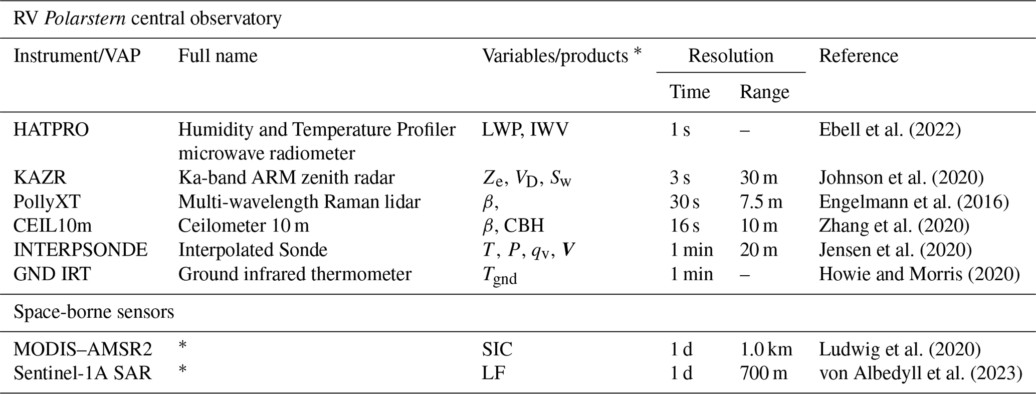
∗ See Appendix D3 for definitions of abbreviations.
The paper is structured as followed: in Sect. 2 the set of instrumentation used for this study on board RV Polarstern is presented. Section 3 gives a detailed description of the methodology developed for the study, and this methodology applied to a case study is presented in Sect. 4.1. The whole MOSAiC wintertime period is statistically analysed and the statistical results for November 2019–April 2020 are presented in Sect. 4.2. Conclusions and an outlook are given in Sect. 5. Supporting material for definitions, methodology, data processing, and further statistical results is summarized in the Appendix.
The suite of atmospheric remote sensing instrumentation on board RV Polarstern relevant for this study is mainly comprised of the Atmospheric Radiation Measurement (ARM) mobile facility AMF1 of the US Department of Energy (http://www.arm.gov, last access: 30 March 2023) and the OCEANET-Atmosphere container (hereafter referred to as OCEANET) of the Leibniz Institute for Tropospheric Research (TROPOS) (Engelmann et al., 2016). A list of instrumentation and data products utilized in this paper, along with their spatial and temporal resolutions and references, is summarized in Table 1. An extensive and detailed description of the data availability of all MOSAiC instrumentation can be found in Shupe et al. (2022), their Table B1.
2.1 Ground-based atmospheric remote sensing
The primary set of ship-based remote sensing instruments for the observation and characterization of clouds are the Ka-band ARM zenith radar (KAZR) and a ceilometer (from ARM) as well as a PollyXT lidar, and a microwave radiometer (MWR) of Humidity and Temperature Profiler (HATPRO) type, both from TROPOS and installed in the OCEANET container.
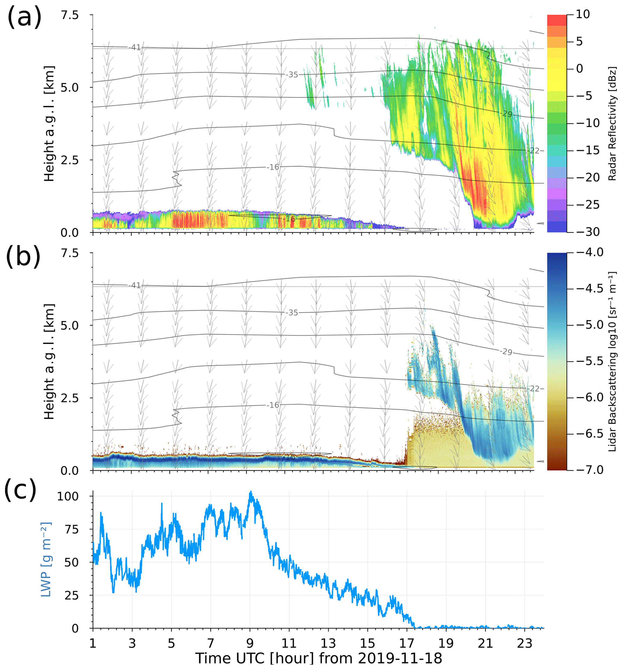
Figure 1Synergistic observations with atmospheric remote sensing instruments on board RV Polarstern from 18 November 2019 during MOSAiC. (a) KAZR cloud radar reflectivity factor; (b) PollyXT lidar backscattering coefficient; (c) microwave radiometer liquid water path (LWP). Shown isotherms (horizontally aligned) and wind vectors (vertical profile lines) were obtained from radiosonde data at selected altitudes and time steps.
Figure 1 shows a typical synergy of observations by the KAZR cloud radar, the PollyXT lidar and the MWR for the case study of 18 November 2019. These synergistic observations together with the atmospheric thermodynamic information provided by weather models are imperative for the cloud type classification and retrieval algorithms for cloud macro- and microphysics as explained in Sect. 3.1.
2.2 Radiosondes
For the characterization of the atmospheric thermodynamic state, the main information is obtained from radiosondes launched from RV Polarstern (Maturilli et al., 2021). For this study, the high-resolution ARM value-added product (VAP) Interpolated Sonde (INTERPSONDE) is used. INTERPSONDE is obtained from linear interpolation of the atmospheric state variables from consecutive soundings into a fixed two-dimensional (2-D) time–height grid. The height and time resolutions are 20 m and 1 min, respectively. The grid extends from 10 m up to 40 km altitude (Jensen et al., 2020). In order to account for the thermodynamic interaction between the surface and the atmosphere, in this study the radiosonde vertical profile has been merged with the ground infrared thermometer (GND IRT; Howie and Morris, 2020) as a proxy for surface skin temperature Tgnd [K], which was assigned to an altitude of 0 m in the radiosonde profile.
Relevant atmospheric state variables needed for our methodology are provided or calculated from the radiosonde, e.g. pressure P [Pa], air temperature T [∘C], specific humidity qv [g g−1], relative humidity [%], wind speed [m s−1], and wind direction [∘] (see Table 1 and references therein). Derived atmospheric state quantities are virtual potential temperature (θv) [K], water vapour transport (WVT) [], the bulk Richardson number (Rib), planetary boundary layer height (PBLH) [m], and cloud-driven mixing layer height (CMLH) [m] above cloud top and below cloud base.
2.3 Satellite-based information for sea ice conditions
Space-borne sensors are the main source of information for long-term and large-scale monitoring of sea ice conditions in the Arctic. For this study, two main sea ice state variables are used: sea ice concentration (SIC) and the lead fraction (LF).
2.3.1 Sea ice concentration
For the observation of sea ice concentration, satellite-borne instruments like the Advanced Microwave Scanning Radiometer 2 (AMSR2) and the Moderate Resolution Imaging Spectrometer (MODIS) are the most reliable instruments in terms of spatial and temporal continuity. These types of instruments, however, have limitations intrinsic to their measurement principles. AMSR2 is a microwave radiometer that is less influenced by clouds than optical sensors and has a good spatial coverage but is limited by its low spatial resolution of about 4 km at 89 GHz or coarser at lower frequencies. On the contrary, MODIS is an optical sensor and offers a higher spatial resolution of 1 km, but its observations are restricted to cloudless conditions. In order to exploit the best features of both sensors, Ludwig et al. (2020) have developed a merged 1 km MODIS–AMSR2 product by tuning SIC from the MODIS 1 km resolution to preserve the AMSR2 average SIC.
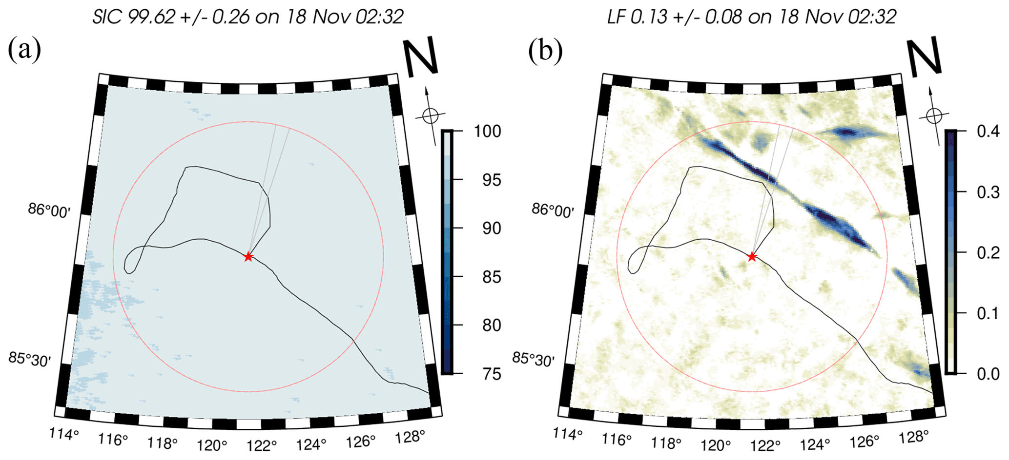
Figure 2(a) SIC from the MODIS–AMSR2 merged product from 18 November 2019. (b) Lead fraction from SAR Sentinel-1. The images are centred on the position of RV Polarstern (red star) on the given date. The RV drift is indicated by the black line; the circle indicates the 50 km radius as the region of interest. The grey cone indicates the relevant observation sector determined by the wind direction at the maximum water vapour transport (see text Sect. 3.4).
The merged MODIS–AMSR2 sea ice product is of particular relevance for the present study since it provides the benefit of potentially detecting open water leads within sea ice due to its finer resolution. We note that leads covered with thin ice, which occur during winter conditions, are not necessarily detected. Nevertheless, for instance, the south–north-aligned sea ice lead on 15 April 2020 observed by Sentinel-1 SAR (Krumpen et al., 2021, their Fig. 3) is resolved by the MODIS–AMSR2 SIC retrieval (Ludwig et al., 2020) but not by the 25 km resolution Ocean and Sea Ice Satellite Application Facility (OSI SAF) product (Lavergne et al., 2016), as shown in Fig. D2a and b, respectively.
Nonetheless, a recent study by Rückert et al. (2023) has shown that warm air intrusion events occurring during the MOSAiC drift in April 2020 fostered the formation of a large-scale surface glazing that resulted in an underestimation of SIC retrievals of about 30 %. This compromises the accuracy of the ARTIST sea ice (ASI) algorithm used by the AMSR2 retrievals (Spreen et al., 2008) and thus also affects the MODIS–AMSR2 product. Therefore, in order to evaluate the accuracy of the MODIS–AMSR2 product, an alternative SIC product needs to be used. Here, the OSI SAF SIC product (Lavergne et al., 2016) was chosen, mainly because of its availability, coverage and higher accuracy during MOSAiC for April 2020 as shown by Rückert et al. (2023). The details of the MODIS–AMSR2 SIC versus OSI SAF product evaluation are described in Appendix C.
2.3.2 Divergence-derived sea ice lead fraction
The satellites Sentinel-1A and Sentinel-1B from the European Space Agency use active microwave synthetic aperture radar (SAR) in the C-band to capture the microwave properties of the sea ice. They are a valuable source to detect leads.
While the most common application is to classify leads from the backscatter coefficient of the SAR scenes (e.g. Murashkin et al., 2018), there is another approach that focuses on the formation process of the leads as seen in sea ice divergence (e.g. Kwok, 2002; von Albedyll, 2022).
By calculating sea ice drift and sea ice divergence from sequential SAR scenes, leads show up in the sea ice divergence whenever the ice moves apart. Such lead fractions from SAR-derived sea ice divergence have the advantage that they indicate the strong local change in ice velocity when a lead opens. They indicate the exact location of leads, they are independent of cloud coverage, and their magnitude is directly linked to the widths of the leads without requiring sensor calibration (Kwok, 2002).
Here, LF is calculated from divergence as described in von Albedyll et al. (2021), von Albedyll (2022), and von Albedyll et al. (2023). The results are interpreted as the average LF per grid cell, which is subsequently drift-corrected and rendered with a spatial resolution of 700 m. One limitation on the lead detection by the divergence-based method is that it only detects new openings. Stationary leads, i.e. leads that do not open or close further, are not detected on the days following the formation even though the leads still exist. Those stationary leads during winter will likely be covered by thin ice. Figure 2 shows a comparison of MODIS–AMSR2 and SAR Sentinel-1 sensors for the sea ice situation on 18 November 2019 around RV Polarstern, illustrating the contrasting capabilities of MODIS–AMSR2 SIC (Fig. 2a) and Sentinel-1 divergence-based LF (Fig. 2b).
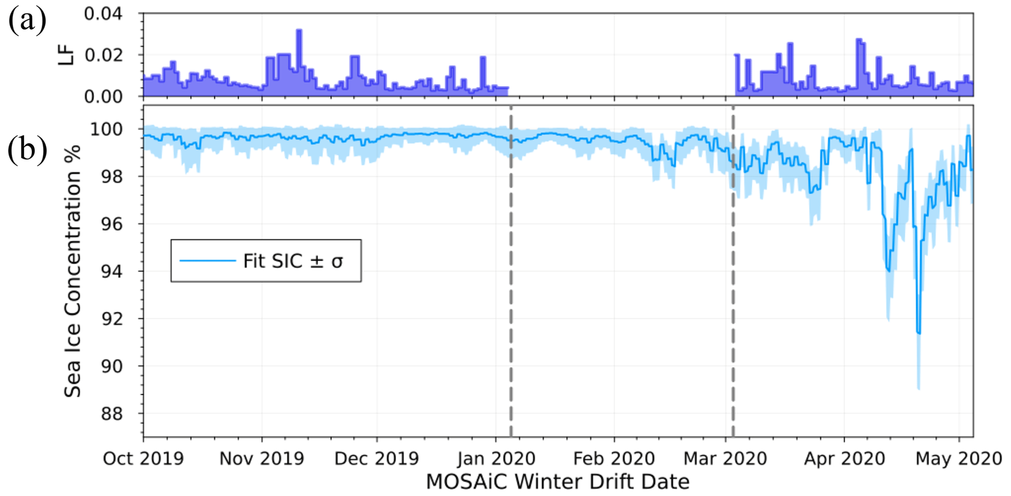
Figure 3(a) Lead fraction (LF) estimated from SAR Sentinel-1 divergence product within 50 km of RV Polarstern central observatory position; note the gap due to a lack of satellite overpasses at RV Polarstern latitude from 14 January 2019 to 13 March 2020; (b) Average fitted sea ice concentration (SIC) from MODIS–AMSR2 retrievals (blue). Shaded area corresponds to the SIC standard deviation of all pixels within 50 km.
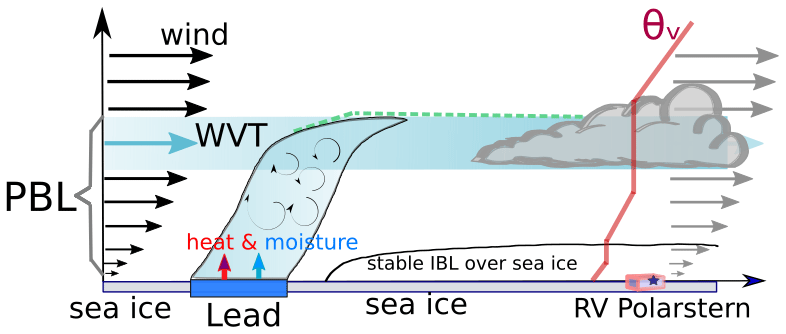
Figure 4Conceptual model explaining how the presence of a sea ice lead can interact with the cloud observed above RV Polarstern. Water vapour transport (WVT) serves as conveyor belt for the latent and sensible heat released by the lead, which can influence the cloud over the measurement site. The thermodynamic and wind profiles are observed above RV Polarstern and considered constant up to the lead location. PBL stands for planetary boundary layer and IBL for intermediate boundary layer.
LF from SAR divergence-based data is available for the study period, except for the time between 14 January and 15 March 2020 (vertical dashed grey lines in Fig. 3), when RV Polarstern was north of the latitudinal coverage extending up to 87∘ N of the Sentinel-1 satellite. To extract the mean LF of a certain region, e.g. 50 km around RV Polarstern (Fig. 3a), the average of all grid cells that are located completely or partly in the region of interest is calculated.
The present study focuses on the MOSAiC expedition from the first to third leg, which ranged from 11 October 2019 to 16 May 2020, thus covering the main part of the transpolar drift though the central Arctic (Nicolaus et al., 2022; Shupe et al., 2022).
To obtain the relevant metrics used to identify the cloud properties that can be associated with effects induced by the presence or absence of sea ice leads, two Arctic observables need to be linked, namely the clouds and the sea ice. This section details the methods applied for this purpose.
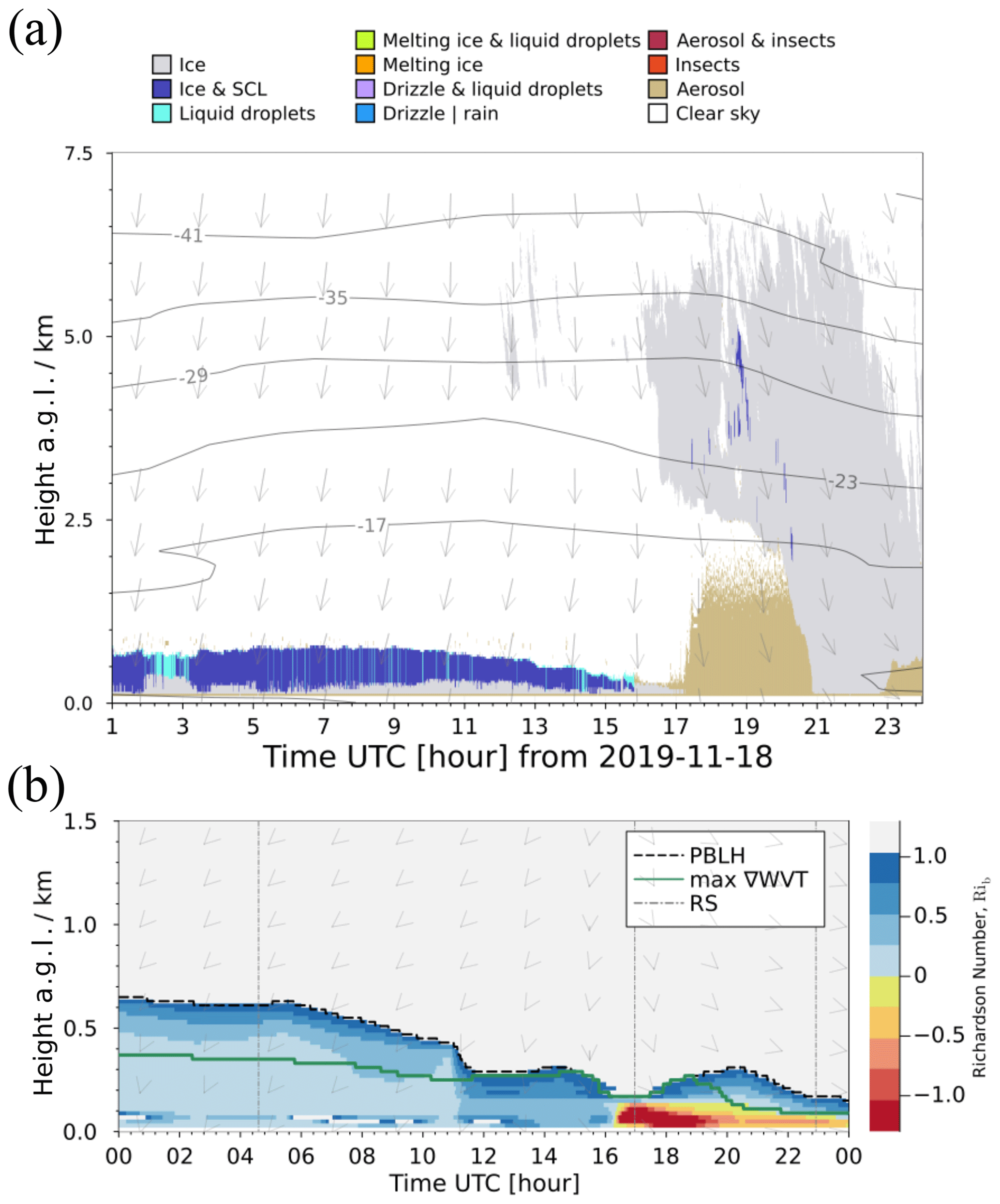
Figure 5(a) Cloudnet classification for RV Polarstern observations on 18 November 2019. Isotherms and wind vectors are obtained from radiosonde profiles. Top colour-coded boxes indicate the type of target classification. (b) Profile of the bulk Richardson number. The selected Ric is visualized by a dashed black line as the PBLH. The dark-green line indicates the location of maximum ∇WVT within the PBLH. Radiosonde launch times are indicated as vertical dash-dotted lines (RS). The wind direction profile is indicated by arrows.
The conceptual model proposed to identify the influence of sea ice leads on the cloud properties observed aloft RV Polarstern's central observatory is depicted in Fig. 4 and described as follows:
-
Leads that are spatially distributed within a 50 km radius of RV Polarstern are considered (Nicolaus et al., 2022).
-
Leads release energy in the form of heat and moisture to the atmosphere (Andreas, 1980; Michaelis and Lüpkes, 2022).
-
This release of energy can initiate a flux of water vapour along the wind direction or feed the horizontal water vapour transport (WVT) that is already present in the atmosphere.
-
Given the proper wind direction, that WVT can move towards the RV Polarstern location.
-
The WVT might favour the formation of new clouds or interact with clouds that already exist by changing their properties.
-
These clouds are then observed at the RV Polarstern central observatory.
According to this concept, the water vapour transport is an important component which serves as a linking mechanism between sea ice leads and the clouds properties observed above the central observatory.
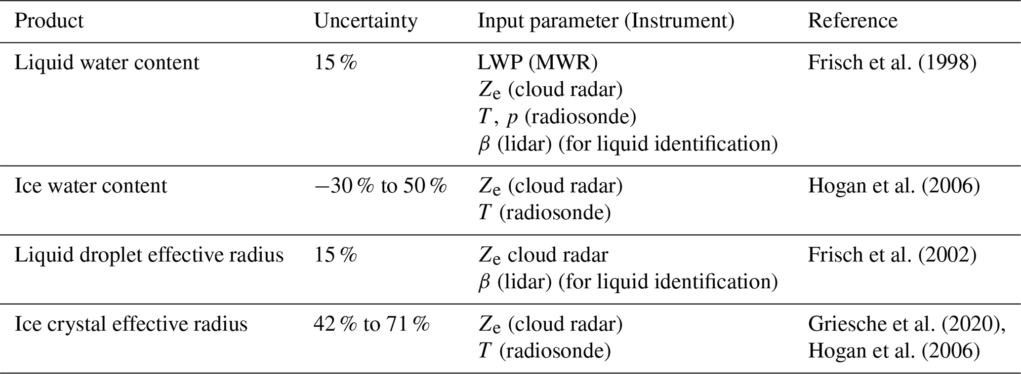
Frisch et al. (1998)Hogan et al. (2006)Frisch et al. (2002)Griesche et al. (2020)Hogan et al. (2006)Table 2Cloudnet product specifications and reference for retrieval methods.
3.1 Cloud classification
The suite of remote sensing instruments, outlined in Sect. 2.1, observing the atmospheric state in the zenith-pointing direction comprises the main source to estimate relevant cloud properties. Several procedures and algorithms have been developed to perform atmospheric target classifications based on synergistic ground-based remote sensing observations (e.g. Shupe, 2007; Wang et al., 2020). Here we make use of the Cloudnet processing chain introduced by Illingworth et al. (2007). Cloudnet is an advanced classification algorithm specifically designed for the continuous evaluation of operational models using state-of-the-art ground-based instruments; Cloudnet provides not only the atmospheric target and cloud-phase classification but also an accurate prediction of the vertical and horizontal distribution of cloud microphysical properties like ice and liquid water content (IWC and LWC, respectively), which are analysed in Sect. 4. The main source of IWC uncertainty comes from the radar reflectivity factor Ze; to have an insight into the uncertainties, an estimation has been made of the relative error for the ice water path (IWP) when the reflectivity is changed by ± 3 %, ± 10 %, and ± 20 % of the original retrieved value. For the case shown in Fig. 5, it can be seen that by modifying the reflectivity by Ze+20 %, the IWP relative error is practically constant with a value of −12 %, while for Ze−20 %, IWP is slightly lower than 13 % of the original retrieved value. For the cases of ± 10 % and ± 3 %, the retrieved IWP lies within a constant margin of ± 6.5 % and ± 1.9 %, respectively, regardless of the absolute value for IWP. Even though this confirms the sensitivity of IWP to the reflectivity factor, it is realistic to assume that the uncertainty in radar reflectivity is within the ± 3 % of measured value, which gives a solid ± 2 % of IWP uncertainty.
Basic requirements for the Cloudnet processing are having observations from a backscattering lidar, a microwave radiometer, and a Doppler cloud radar. Cloudnet is continuously being improved and developed by a large community of users under an open-source scheme (https://cloudnet.fmi.fi, last access: 30 March 2023) hosted by the Finnish Meteorological Institute and coordinated by the ACTRIS initiative (https://www.actris.eu, last access: 30 March 2023). Cloudnet has been selected as a classification algorithm for this study in its open-source version developed by the ACTRIS consortium (Tukiainen et al., 2020). Table 2 lists the input parameters and retrieval products obtained from Cloudnet, and Table 1 lists the instrumentation used with Cloudnet in the present work.
Figure 5a synthesizes an example of Cloudnet classification capabilities adapted to observations during MOSAiC, in addition to the target classification. The presented case study of 18 November 2019 shows that the stratiform low-level cloud present until 17:00 UTC mostly consists of a mixture of supercooled liquid droplets and ice particles, while the deep cloud system (present from 19:00 UTC onwards in Fig. 1) is mostly classified as ice-only.
A limitation of the Cloudnet classification and other synergistic retrievals happens in situations when the liquid cloud base is located below the first radar range gate, meaning the lidar signal is attenuated by low-level liquid clouds. This hampers the proper classification of liquid layers for which a lidar signal is required; hence all clouds are classified as pure ice clouds. This situation can be seen, for example, in Fig. 7b from 16:00 to 17:00 UTC and Fig. D1d (from 14:30 to 18:00 UTC). For the MOSAiC wintertime period, about 29 % of observed clouds were found to have bases below the first radar range gate; they were classified as low-level stratus according to the methodology developed by Griesche et al. (2020) based on information from the signal-to-noise ratio of the PollyXT 532 nm near-range channel.
3.2 Atmospheric water vapour transport
The transport of air masses in the atmosphere is the main mechanism for the interaction of water vapour with the cloud characterized as in Sect. 3.1. One widely used concept to describe intense filament-like vapour transport in the atmosphere is the one of atmospheric rivers (ARs) (Martin-Ralph et al., 2020). Typically, either the vertically integrated water vapour (IWV) or integrated vapour transport (IVT) defined by Eq. (B1) in Appendix B is analysed to characterize ARs. Commonly ARs are identified whenever vapour flux exceeds a defined threshold relative to the zonal mean (Martin-Ralph et al., 2020; Zhu and Newell, 1998). One disadvantage of both AR characteristic variables is that IVT – being an integrated quantity – does not carry the information about the location of vapour transport in the vertical or whether one or multiple layers of vapour fluxes are present at different altitudes. The same is true for the IWV, with an additional limitation being that IWV is a wind-independent variable, and thus no transport is implicit with this metric.
For the present study, however, it is of primary interest to monitor the transport of water vapour in the lower layers of the atmosphere where the interaction with sea ice or open ocean is mostly taking place. That is why a detailed analysis of the vertical changes in vapour transport in the lower atmosphere becomes of paramount interest to locate where the most relevant flux is located. To do so, we derive the vertical gradient of WVT starting from the standard definition of IVT (Martin-Ralph et al., 2020) given by Eq. (B1), detailed in Appendix B. The vertical gradient of WVT (∇WVT) is calculated using radiosonde profiles of specific humidity qv [g g−1], horizontal wind speed vw [m s−1], and air pressure P [Pa], with all these at altitudes z [m], following Eq. (1), whose detailed derivation is described in Appendix B:
where g is the constant of gravity and ∇ indicates the vertical gradient.
The advantage of using Eq. (1) is threefold: first, the altitudes at which local maximums of WVT occur can be identified separately from the flux profile; second, there is no need for thresholds to identify whether or not a layer of WVT is present (as is the case for IVT); and third, the derivative component behaves as a weighting factor (inverse exponential with altitude) that naturally gives more weight to fluxes at the lowest layers and diminishes the upper ones where meso-scale ARs are more likely to be present. To constrain the relevant atmospheric layer even more, the ∇WVT profile is analysed only below the planetary boundary layer height (PBLH; estimation is explained in the following subsection). This allows us to dismiss ∇WVT peaks that are less likely to have interacted with sea ice in the vicinity of RV Polarstern.
3.2.1 Estimation of the planetary boundary layer height
The Richardson number is defined as the ratio of turbulence associated with buoyancy to that associated with mechanical shear. This ratio resolved at increasing altitudes above surface level is known as the gradient Richardson number (Ri), and it is widely used to estimate the planetary boundary layer (PBL). However, when the atmospheric turbulence profile cannot be resolved with measurements at spatial and temporal resolution that is sufficiently high to resolve small-scale turbulence – as in the case with sounding the atmosphere – it is more convenient to use the bulk Richardson number (Rib) as a good indicator of the stability conditions in the atmosphere. The bulk Richardson number is defined as in Eq. (2):
where g is the constant of gravity acceleration 9.81 [m s−2]; θv is the virtual potential temperature profile [K], ; and and are the horizontal wind components [m s−1]. , with z being the altitude of the atmosphere layers [m] and the subscript 0 indicating the surface reference.
The atmospheric stability is characterized by a range of values of Rib, with Rib<0 indicating an unstable and turbulent atmosphere, Rib<Ric a neutral atmosphere, and Rib≥Ric a stable with almost all turbulence diminished; here Ric is the critical Richardson number. To estimate the PBLH by means of Rib, the standard procedure relies on applying Ric as a threshold that defines the layer above which the atmosphere is considered to be non-turbulent and laminar. The most common Ric value used is 0.25 although there is a wide range of values that can be found in the literature, spreading from 0.1 to 1. For this study θv(z0) and Rib have been calculated using the radiosonde data in combination with the ground infrared thermometer Tgnd (GND IRT) as surface skin temperature. For the purpose of this study, an exact estimation for the PBLH is not crucial, but rather a rough approximation is useful as an atmospheric layer top to be considered for the determination of the altitude at which ∇WVT reaches a local maximum. The top of the PBL is then considered to be located at the altitude when the condition Rib≥1 is first met, with 1 being a rather conservative critical value to cover most of the relevant mixing layers for the Arctic winter atmosphere.
In Fig. 5b the atmospheric stability based on the bulk Richardson number given by Eq. (2) and calculated from the ARM INTERPSONDE product is depicted for the 18 November 2019 case study. The atmospheric stability is colour-coded by light- to dark-blue colours (0 < Rib < Ric) for a statically stable to neutral atmosphere. Above the critical value Ric=1 (light grey), the atmosphere is not considered to be significantly turbulent anymore, therefore the cloud within or above this level does not have the potential to mix with the layers below. Unstable atmospheric conditions are highlighted by the yellow to red colours corresponding to sub-zero Rib values, which, for the case of 18 November 2019, occur once the wind direction shifts to northerly and northwesterly directions and the deep cloud system is observed above RV Polarstern. For this case, the maximum of ∇WVT within the PBLH varies between 0.1–0.4 km, which is depicted by the solid green line in Fig. 5b.
In the following section, it is explained how ∇WVT is exploited as the mechanism responsible for the interaction between sea ice or open ocean and the cloud observations above RV Polarstern.
3.3 Cloud coupling
3.3.1 Cloud mixing layer
The cloud-driven mixing layer below the cloud base is determined by calculations based on the degree of variability in the virtual potential temperature θv profile (Eq. A1). A quasi-constant θv profile below cloud-base height (CBH) implies a well-mixed layer. A departure from quasi-constant θv indicates a thermodynamic inversion and thus decoupling from the layer beneath.
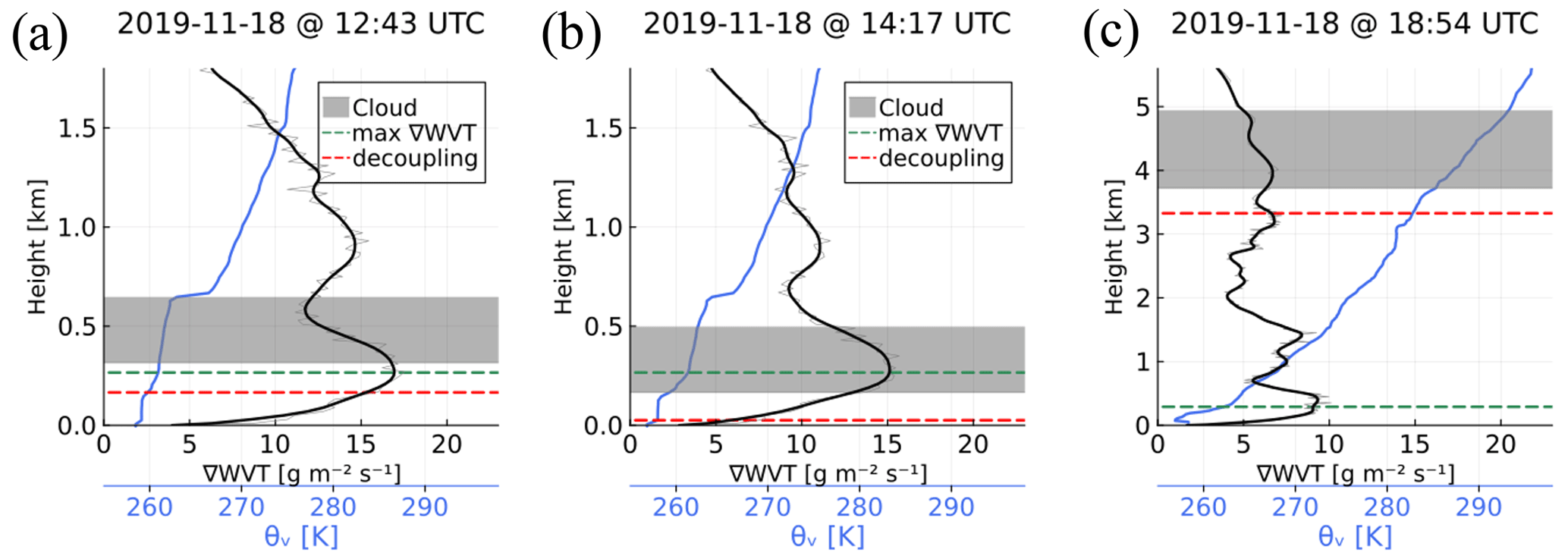
Figure 6Examples for ∇WVT profile (black axes) coupling (a, b) and decoupling (c) to the cloud for 18 November 2019. The liquid cloud layer is shown as a grey-shaded area. The coupling status is determined by the position of the maximum ∇WVT (dashed green) relative to the decoupling height CMLH (dashed red): (a) the max ∇WVT is above CMLH and below the cloud base but is still considered coupled to the cloud and (b) max ∇WVT is inside the cloud. Panel (c) shows a case where the cloud is decoupled. For reference θv is indicated by the solid line, and the x axis is in blue.
To estimate the cloud mixing layer height (CMLH) the relative variability in θv starting at the cloud base ad going downwards is analysed. This concept has been extensively utilized by Sotiropoulou et al. (2014) and Gierens et al. (2020) for classification of surface-coupled clouds. The criterion used in this study consists of calculating the cumulative variance of θv(i) ( defined by Eq. A2) starting from the cloud base and going towards the surface level or i = 0. Thus CMLH is equal to the z value at which the criterion is first met. The same procedure is applied to estimate the cloud-driven mixing layer above the cloud top. The CMLHs below and above the cloud base and -top are quantities used to estimate the coupling or decoupling state of the cloud with the water vapour transport, as described in the following section.
3.3.2 Cloud coupling classification
The observations are sorted into two classes depending on the likelihood of interaction between the sea ice situation upwind and the cloud observed aloft, and they are linked by the water vapour transport as a conveying mechanism for moisture and sensible heat to the clouds above the central observatory, i.e. whether or not the WVT is coupled or decoupled to the cloud. A cloud observation is considered to be coupled to WVT when the location of maximum ∇WVT is found to meet one of the following criteria: be in the cloud, or between the cloud's CMLH below and above the cloud base and top, respectively. Conversely it is considered decoupled when the maximum of ∇WVT happens to be either above the cloud top's CMLH or below the cloud base's CMLH. Those cases are illustrated in Fig. 6 for coupled (Fig. 6a and b) and decoupled (Fig. 6c) situations. It is important to note that in the present study we are departing from the canonical concept of surface–cloud coupling generally found in the literature. This is due to the fact that the location of sea ice lead occurrence is not strictly co-located with the position of RV Polarstern (see for instance Figs. 2 and D2); thus the sea ice–cloud interaction is not expected to take place vertically within a static column but rather to be dynamically ascribed by the air mass movement from afar. Moreover, the persistent presence of a surface temperature inversion in the Arctic makes the case of a vertically static column cloud–surface coupling a rare event.
Hence our definition of the sea ice–cloud coupling status is governed by the following criteria:
- I.
Coupled. This is when the maximum of ∇WVT is localized within the cloud-driven mixed height above and below the cloud top and base, respectively, in Fig. 6a and b.
- II.
Decoupled. This is when the maximum of ∇WVT is found to be outside the cloud layer limited by the top or bottom CMLH. as shown in Fig. 6c.
According to the above, the classical definition of cloud–surface coupling is only a special case of this more general approach when the CMLH below the cloud base reaches the surface level; i.e. z=0 in Eq. (A2). We found, however, that during the MOSAiC wintertime, this situation only comprises 4.7 % of all cloudy observations and 7.3 % of all cases that fulfil criterion (I), “coupled”.
3.4 Sea ice concentration in the direction of WVT
Information about the state of the sea ice is considered within a circular area of 50 km radius centred on the RV Polarstern. This particular radius has been chosen as a compromise to cover the sea ice conditions representative of the observations at the central observatory based on SIC comparisons of circles with 6, 50, and 100 km radius (see Krumpen et al., 2021).
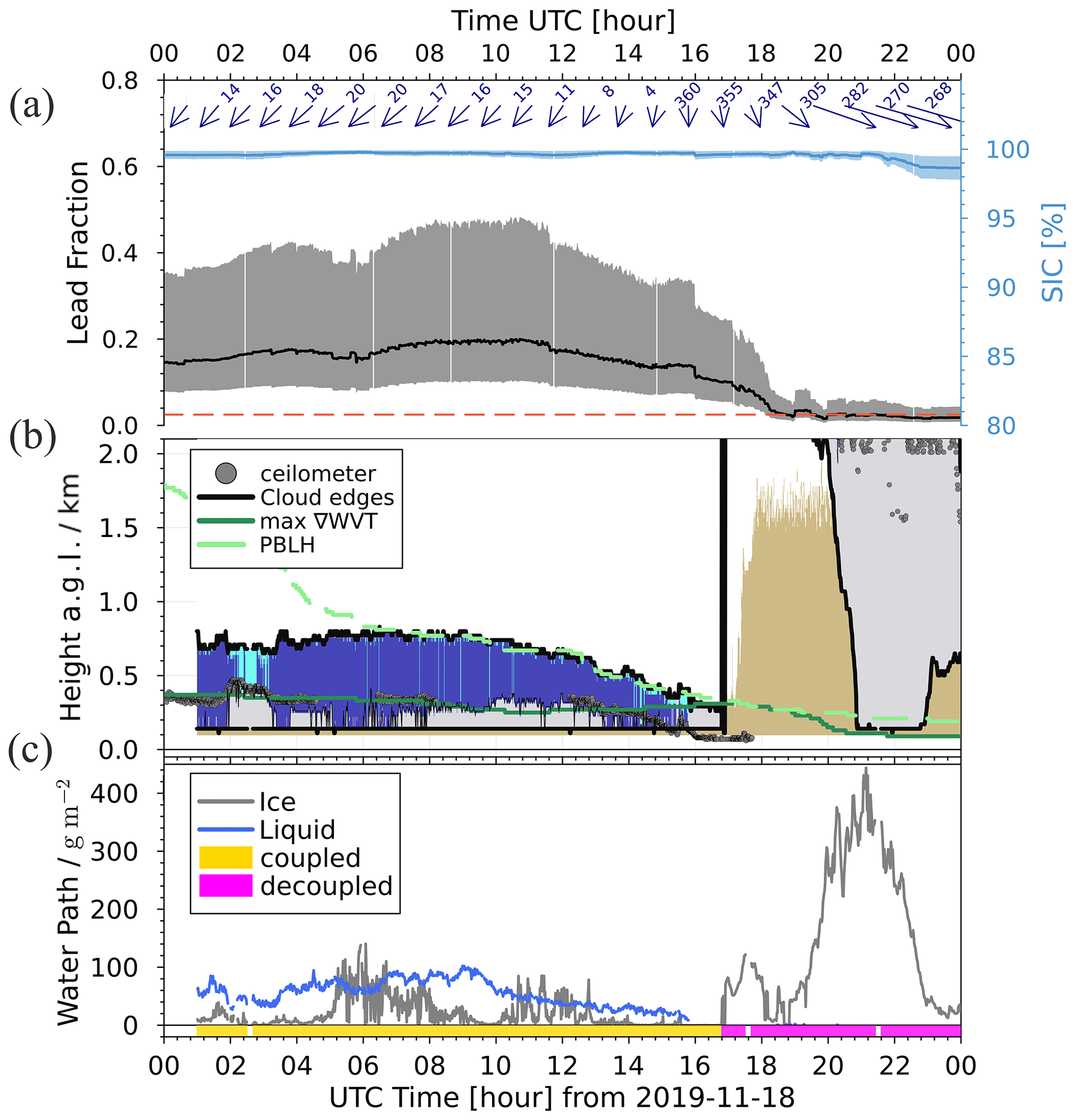
Figure 7From top to bottom: (a) median lead fraction time series (black line, left axis) with the interquartile region (shaded region) and sea ice concentration (light blue, right axis) after considering only grid cells within a conical sector centred on RV Polarstern. The direction of the conical sector as a function of the wind direction is shown by the blue arrows and values on top. The horizontal dashed red line indicates an average LF value for totally covered sea ice. (b) The same as Fig. 5 but magnified to the lower 2 km where the post-processing cloud edge detection is highlighted with black lines and the lidar cloud base is shown in grey dots. The height of maximum ∇WVT is shown in dark green, and the PBLH is in light green (dashed). (c) IWP and LWP within the detected cloud layer (b). The coupled–decoupled status flag is highlighted in yellow and magenta, respectively.
Within the 50 km circular area, sea ice conditions relevant for the interaction with the cloud observations are extracted from a conical sector centred on RV Polarstern and extended up to a 50 km radius and angular span of 5∘. The azimuth angle of this conical sector is adjusted every minute based on the wind direction measured at the altitude of maximum ∇WVT (green lines in Figs. 6 and 5b). For instance, for the sea ice situation on 18 November 2019 only the LF and SIC highlighted within the grey lines in Fig. 2 are associated with the zenith-pointing cloud observations. To ensure that the considered wind direction is still representative within the 50 km range, back-trajectory analysis was performed using the Lagrangian back-trajectory tool LAGRANTO (Sprenger and Wernli, 2015). The trajectory of WVT was tracked backwards from the altitude where maximum ∇WVT occurs; it was found that the back trajectories show a considerable agreement with the assumed wind direction within the 50 km radius (see Supplement).
Although RV Polarstern's ice floe drifted (i.e. the geographical position for the centre of the 50 km circular area had an average drifting speed of 8.52 km d−1; Krumpen et al., 2021; Nicolaus et al., 2022), we update the azimuth angle of the sea ice conical sectors every minute in synchrony to the available vertical wind profiles given by ARM's INTERPSONDE product. Since LF and SIC information is only available on a daily basis, the centre of the 50 km circular area also needs to be updated accordingly to avoid abrupt changes in the relative position of the leads with respect to RV Polarstern.
4.1 Case study of 18 November 2019
Besides the Cloudnet retrieval products summarized in Table 2, further macro-physical and thermodynamical properties of the cloud are estimated from the Cloudnet target classification and from radiosonde. These properties include cloud-base height and cloud-top height (CBH and CTH, respectively) as well as the temperature at the cloud base and top. Figure 7 summarizes all those properties as well as the coupled–decoupled status of every observation according to Sect. 3.3 for the case study of 18 November 2019. Results presented in Fig. 7c are based on vertical integrals from single-layer CBH to CTH of Cloudnet-determined LWC and IWC (see Table 2). LWP is determined for liquid-only clouds and MPCs, whereas IWP is determined for MPCs and pure ice clouds and includes falling solid precipitation (snowfall).
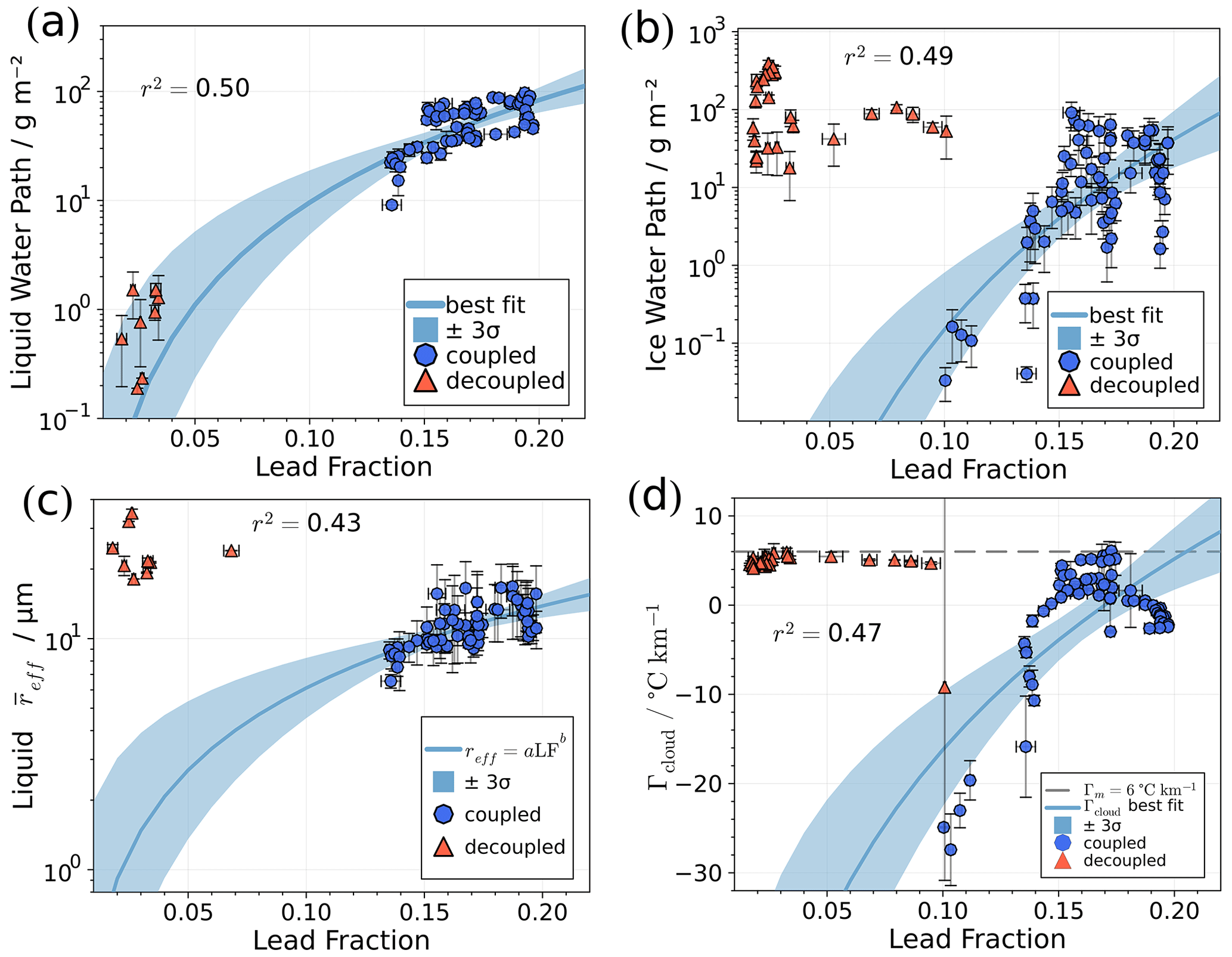
Figure 8Results for 18 November 2019: single-cloud-layer relationships between LF and micro- and macro-physical cloud properties. Observations are represented as averages (circles and triangles) with standard deviation (bars) within intervals of 15 min; coupled and decoupled cases are marked as blue circles and orange triangles, respectively. (a) Mean single-cloud-layer LWP vs. LF (black line in Fig. 7, top panel). (b) The same but for IWP of the same cloud layer. (c) Cloud layer average effective radius for liquid droplets. (d) Γcloud as defined in Eq. (4) vs. LF; the horizontal dashed line represents a moist adiabatic Γm. In all panels the best fit is shown as a dark-blue line and the corresponding coefficient of determination r2 is based only on coupled data points.
The case study in Fig. 7a shows the corresponding 1 min resolution time series for the sea ice statistics of all grid cells located within the conical sector aligned with the wind direction (see grey cone in Fig. 2) as described in Sect. 3.4. The conical sector is adjusted as a function of the wind direction (blue arrows in the top panel of Fig. 7) given at the height of maximum ∇WVT occurrence (Fig. 7b, solid green line).
From 00:00 to 16:00 UTC on 18 November 2019, latent heat and sensible heat were advected towards RV Polarstern from north-northeasterly directions where a sea ice lead had formed (Fig. 2, right panel). LF within the conical sector has median values ranging from 0.1–0.2 and with an interquartile region (IQR) of up to 0.4 shown in Fig. 7 (top panel). During this time period of high LF, a stratiform low-level MPC was observed (Figs. 1, 5a, and 7b).
At approximately 16:00 UTC, the wind direction changed towards the northwest to west, where no leads were located. This cut-off of the heat and moisture supply led to dissipation of the low-level MPCs. After about 17:00 UTC, a deep cloud system related to a storm was observed above RV Polarstern. This storm was associated with sublimation just above the maximum ∇WVT and also led to an increase in turbulence in the lowest atmospheric layers (see Fig. 5b, red colours). SIC shows a slight decrease from values near 100 % to about 98 % towards the end of the case study period. The coupling status is highlighted by the yellow (coupled) and magenta (decoupled) flag at the bottom of Fig. 7c.
From Fig. 8a, a relationship between LWP and LF can be seen; i.e. the larger the LF, the higher the LWP. For IWP (Fig. 8b), a more scattered relationship is found, with a wide range of IWP values occurring independently of the magnitude of the observed LF. The only clear feature is the clustering of larger IWP values at low LF which correspond to the decoupled profiles of the deep cloud present after 17:00 UTC. Note that between 16:00 and 17:30 UTC (in Fig. 7b) the lidar detects a liquid layer below the lowest available Cloudnet classification height, meaning Cloudnet could not relate this period with the occurrence of liquid droplets but instead misclassifies it as ice cloud only. This is reflected in the total water path calculated within the lowest and top cloud limits as indicated in Fig. 7c.
Table 3Number of available observations at 1 min resolution during the MOSAiC wintertime for the statistical analysis. The total of observations includes cloudless and cloudy cases. For cloudy situations, a distinction is made between WVT coupled and decoupled. The frequency of occurrences of different intervals of cloud water path sorted by the coupling status is presented in Appendix D2, Fig. D3a.
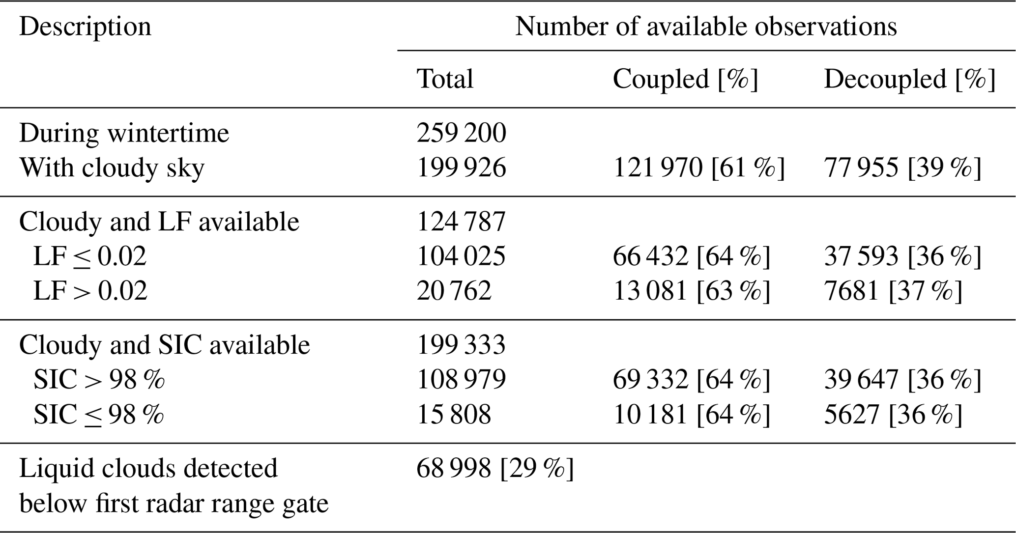
Figure 8c depicts the liquid effective radius retrieved by Cloudnet and averaged over the cloud layer defined by
where N(z) is the droplet number concentration and re(z) is the effective radius corresponding to the altitude z within CBH and CTH. The best-fit curve indicates a slightly positive correlation as LF increases.
Shown in Fig. 8d is the in-cloud temperature lapse rate defined as follows:
Figure 8d indicates that Γcloud is often close to the moist adiabatic lapse rate of 6.0 (dashed horizontal line in Fig. 8d), especially the decoupled cases (orange triangles) independent of LF. The negative Γcloud values represent cases with a temperature increase within the cloud layer or inversion at the cloud top, and they are mostly related to coupled clouds (blue circles).
The 18 November 2019 case study encompasses a situation where the observed clouds have a well-defined correlation with LF situation upwind, mainly due to the occurrence of a single cloud layer. This is not always the case, as can be seen in Fig. D1, where the cloud properties correlated to LF are more subtle. To assess the robustness of the case study results over a wide range of cases, a statistics analysis is performed based on the same methodology applied to the whole wintertime MOSAiC expedition.
4.2 Statistical analysis
The methodology introduced for the case study in Sect. 4.1 was applied to the whole wintertime MOSAiC period (November 2019–April 2020). Table 3 summarizes the obtained dataset that was statistically analysed after splitting between cases with LF less than or equal to 0.02 (LF ≤ 0.02) and LF greater than 0.02 (LF > 0.02). In that way we try to isolate cases in which sea ice leads have most likely been interacting with the observed clouds. The motivation to separate the coupling state when LF ≤ 0.02 is to have an insight into situations where WVT is present and leads can be located at ranges further than 50 km. In the following analysis when the probability distribution function (PDF) of a certain cloud property shows a similar shape for coupled cases with LF ≤ 0.02 and LF > 0.02, it might imply that leads located further away produce similar PDFs, e.g. having the same PDF maximum location but being less frequent. On the contrary, when the PDFs are different for cases of coupled with LF > 0.02 and decoupled (e.g. multiple peaks versus mono-modal distributions), it is an indication that the leads–WVT–cloud coupling system is separating the observations into two distinguishable distributions. This section presents the relevant statistical differences in relation to the cloud micro- and macro-physics and thermodynamic properties between clouds classified as coupled or decoupled to the WVT.
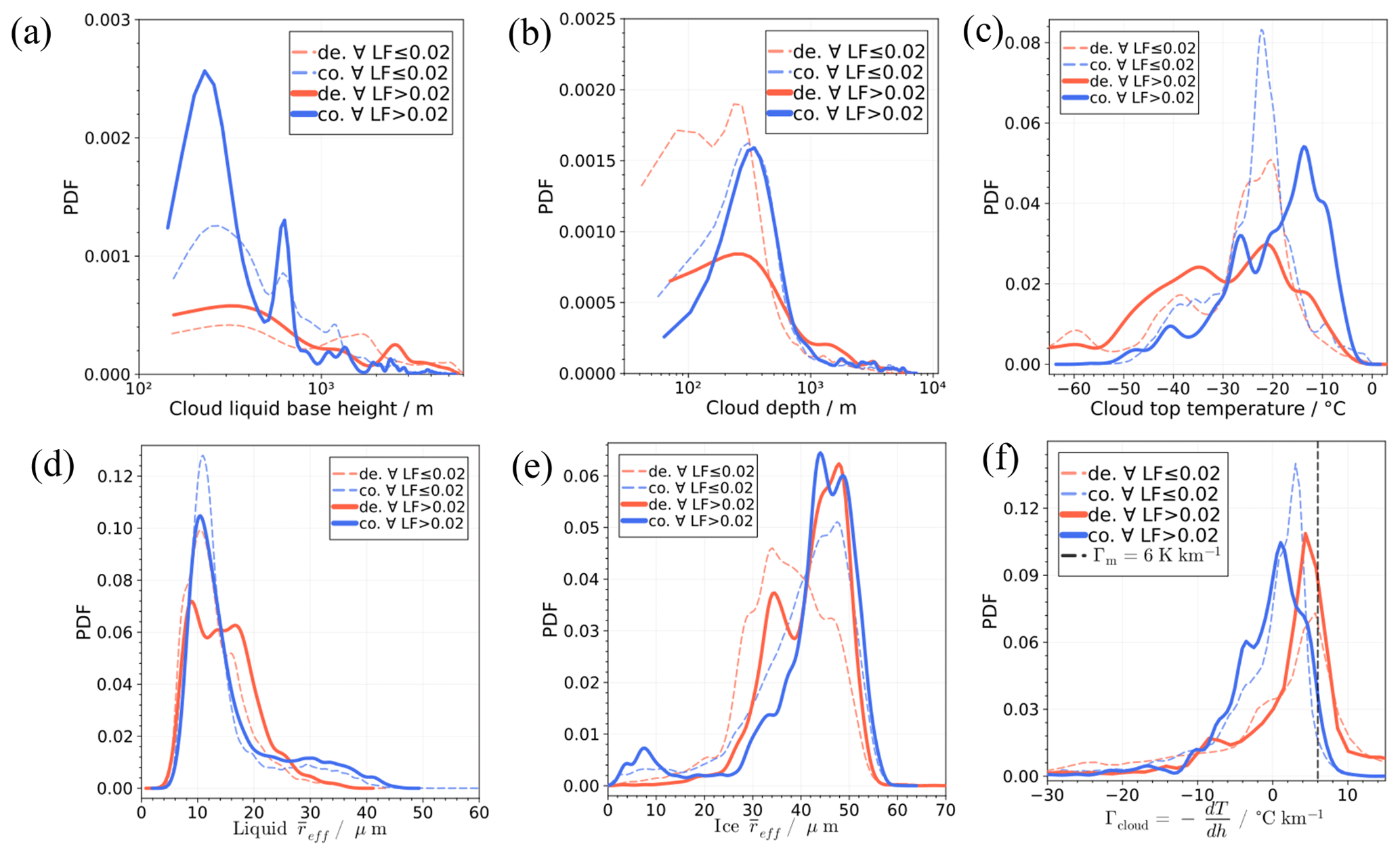
Figure 9Probability distribution functions for all observations from November 2019 to April 2020. Data are sorted by LF ≤ 0.02 (dashed lines), LF > 0.02 (solid lines), coupled (“co.”, blue), and decoupled (“de.”, orange) cases of cloud properties. (a) For liquid layer base height, separated for coupled (blue lines) and decoupled (orange lines) cases. Dashed lines correspond to LF ≤ 0.02 and solid lines to LF > 0.02. (b) The same but for the cloud depth. (c) PDF for cloud-top temperature. (d) PDF for cloud layer mean effective radius of liquid droplets. (e) Cloud layer mean effective radius of ice crystals. (f) In-cloud temperature lapse rate, with the dashed black line indicating a nominal moist adiabatic lapse rate.
Figure 9 depicts the PDFs of different macro- and microphysical cloud properties. The data are separated into four groups: WVT coupled cases (blue), decoupled cases (orange), cases with LF ≤ 0.02 (dashed lines), and cases with LF > 0.02 (solid lines). In Fig. 9a the PDFs of the liquid layer base height presented for coupled cases are generally comprised of low-level clouds with a probability of occurrence significantly enhanced for the subset corresponding to LF > 0.02, with a main peak at 250 m. In contrast, decoupled clouds do not have a pronounced peak in liquid layer base height occurrence but are more homogeneously distributed over a range of a few hundred metres to 1 km. Furthermore, Fig. 9b exposes the fact that coupled clouds also tend to be thicker, with a peak in the PDF at around 400 m, whereas decoupled clouds are equally likely to have thicknesses ranging between 40 and 500 m. Statistics of cloud-top temperature are shown in Fig. 9c, where two distinct features appear: clouds related to LF ≤ 0.02 have a maximum probability of cloud-top temperature at around −22 ∘C regardless of their coupling state. Conversely, for LF > 0.02, coupled clouds are generally warmer with their maximum PDF of cloud-top temperature at about −12 ∘C and a second minor PDF peak at −29 ∘C. For decoupled clouds and LF > 0.02, the cloud-top temperature PDF spreads out to colder temperatures with a primary peak at −22 ∘C and a second peak at −36 ∘C. Moreover cloud-top temperatures below −40 ∘C are considerably more frequently observed for decoupled than coupled clouds.
In Fig. 9d the PDF of the cloud layer mean liquid droplet effective radius of coupled cases peaks at 12 µm for both LF classes. The PDF of for the WVT decoupled cases exhibits a bimodal distribution peaking at 8 and 17 µm irrespective of LF. Likewise, the average effective radius for ice particles (Fig. 9e) exposes a bimodal PDF of ice with peaks at 42 and 49 µm almost equally likely to occur for coupled cases, while the PDF for decoupled cases has one minor peak at 32 µm and a major peak at 48 µm. The PDFs for LF ≤ 0.02 (dashed lines) have single maximums at 48 and 32 µm for coupled and decoupled cases, respectively.
To complement the thermodynamic features of the cloud, Fig. 9f shows the PDF of the cloud layer temperature lapse rate. The main feature found is that for LF ≤ 0.02, the decoupled PDF indicates a maximum at the nominal value for the moist adiabatic lapse rate Γm, while decoupled clouds at LF > 0.02 show a slightly lower lapse rate.
The coupled Γcloud PDFs are biased and skewed towards negative lapse rates with the most probable values found to be 0 and −2 for LF ≤ 0.02 and LF > 0.02, respectively. The latter also has a minor peak in the PDF at around −5 . The dominant feature found in Fig. 9f is that the Γcloud PDFs of clouds coupled to the WVT mechanism are displaced towards lower or even negative Γcloud values (i.e. temperature inversion above the cloud base), and this characteristic is enhanced when LF > 0.02.
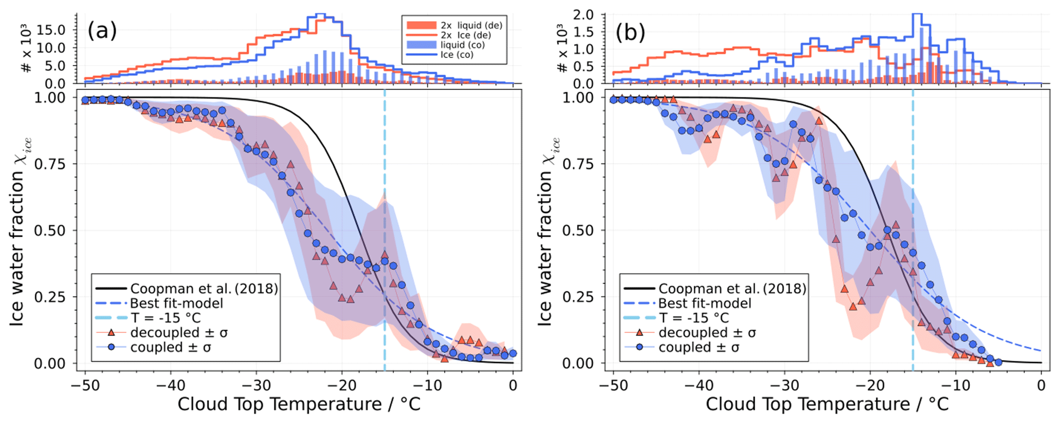
Figure 10Top panels: histograms of the number of occurrences for liquid (bars) and ice (lines) water paths for coupled (“co”, blue) and decoupled (“de”, orange) cases. For visualization purposes, the decoupled number of occurrences has been scaled by 2 (2×). Bottom panels: ice water fraction, as defined by Eq. (5), versus cloud-top temperature for (a) all cases and (b) cases where LF > 0.02. Coupled (decoupled) cases are depicted as blue circles (orange triangles); shaded areas represent 1 standard deviation of the ice water fraction sorted within 1 ∘C temperature bins. The best fit to the coupled data is shown as a dashed blue line.
4.2.1 Fraction of ice water content in cloud
Hereafter we define the fraction of ice water content in the clouds relative to the total condensed water in the cloud (ice and liquid) as follows:
The definition given in Eq. (5) is in line with the Korolev and Milbrandt (2022) phase composition of clouds but differs from most of the studies based on space-borne Arctic observation (Coopman et al., 2018) where χice is defined as the number of grid cells considered to be ice divided by the number of grid cells considered to be either liquid or ice. Similarly, the definition in Eq. (5) differs from other ground-based and ship-based observations over mid-latitudes and the Arctic, where the fraction of ice-containing clouds with respect to all observed clouds is considered (Kanitz et al., 2011; Westbrook and Illingworth, 2011; Griesche et al., 2021) regardless of the water content in those clouds. Therefore the results based on ice water fraction analysis presented here cannot be directly related to the previously mentioned work. We are mainly interested in the features controlling the cloud microphysical properties such as LWP and IWP, since those are the dominant drivers of the cloud–surface interaction. Furthermore, note that in the following analysis, Eq. (5) is only applied to the single cloud layer relevant for the classification of coupled or decoupled to the WVT; therefore the results are not representative of the whole atmosphere in the case of multi-layer cloud situations.
Figure 10 depicts a clear difference in the ice water fraction when separated by the cloud coupling to the WVT status (blue for coupled and orange for decoupled) between −15 and −25 ∘C for cases with LF ≤ 0.02 (a) and between −12 and −30 ∘C for cases with LF > 0.02 (b). For the situation in (a) the ice water fraction, for coupled and decoupled cases, increases until a local maximum corresponding to a cloud-top temperature of −15 ∘C is reached, as indicated by the vertical dashed light-blue line. This can be explained by the fact that at approximately −15 ∘C the maximum ice growth takes place due to the largest difference between saturation water vapour pressure over ice and water (Rogers and Yau, 1991). Below −15 ∘C cloud-top temperature, the coupled and decoupled cases depart significantly until approximately −25 ∘C, with the coupled cases showing a steady increase in ice water fraction, presumably due to the intake of humidity provided by the coupling with the WVT and thus fostering the formation of ice particles, whereas the decoupled case indicates a drop of ice water content up to χice = 25 % at a cloud-top temperature of −20 ∘C, whereafter the heterogeneous freezing process continues. Both χice curves reach 50 % at about the same temperature of −22 and −24 ∘C for the decoupled and coupled cases, respectively. For χice = 75 % and higher, the coupled and decoupled χice curves behave similarly towards homogeneous freezing, which has been found to occur within the range −37 to −40 ∘C (Rogers and Yau, 1991; Pruppacher and Klett, 1997).
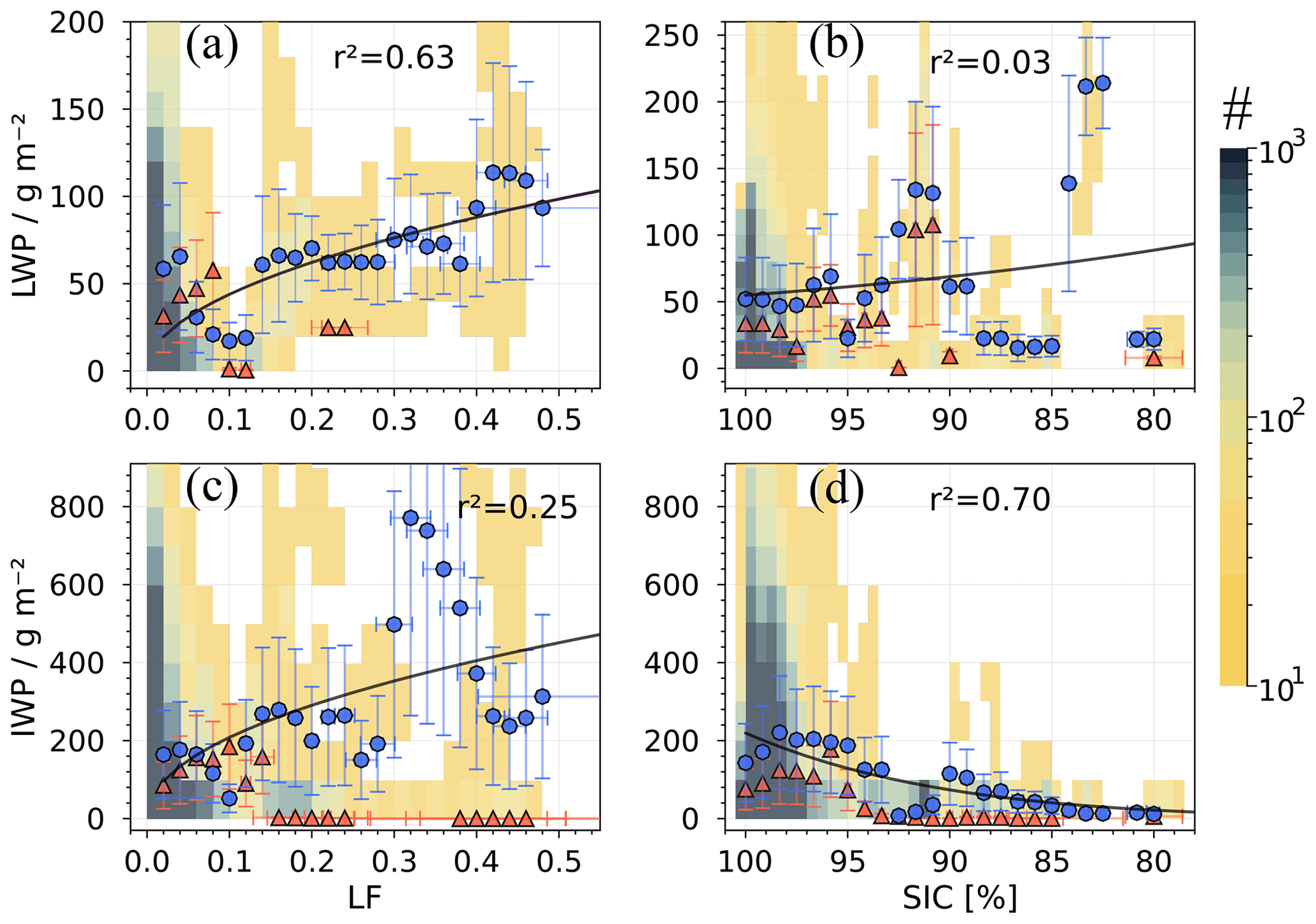
Figure 11Data for the period November 2019–April 2020: top row (a, b), distribution of LWP as a function of observed LF (a) and SIC (b); bottom row (c, d), distribution of IWP as a function of LF (c) and SIC (d). The symbols are the average of the observations within a fixed LF bin width, while the bars indicate 63 % variability within the LF bin. The colour scale indicates the number of observations within the bins for the whole dataset, whereas the symbols represent only the data corresponding to LF > 0.02. The coupling status is indicated by orange triangles (decoupled) and blue circles (coupled). The black curves represent the best fit for only the coupled blue circles, and the coefficient of determination is given by r2.
For the subset of data with LF > 0.02 (Fig. 10b), the χice coupled and decoupled cases reach a first local maximum at a colder temperature of −18 ∘C. Note, however, that the number of cases for LF > 0.02 are much smaller by a factor of ∼ 6 (Table 3). Furthermore this local maximum at −18 ∘C coincides with χice = 50 %, which means it reaches the 50 % ice water fraction at a warmer temperature as compared to Fig. 10a. Moreover, it can also be seen that χice for LF > 0.02 follows more closely the empirical model given as by Coopman et al. (2018) based on satellite-based observations for the Arctic between 2005 and 2010 during March to September. A slight modification to the empirical model for χice was made in this study so that β1 fits the temperature corresponding to χice = 50 %. The decoupled curve shows a steep drop in the ice fraction to a minimum of about 15 % at the temperature of −20 ∘C (a similar situation to that observed in Fig. 10a), followed by an abrupt increase in χice to 95 %. The best-fit curve for χice values of coupled cases has a more monotonic increase but with a less steep slope than the empirical model (dashed blue curve).
4.2.2 Liquid and ice water content as a function of sea ice
With the aim to confirm the relationship between cloud properties with the sea ice lead fraction found in Sect. 4.1, the whole dataset is analysed and summarized in Fig. 11. The number of occurrences for the whole dataset of observations containing either ice or MPCs is shown colour-coded in the background (corresponding to the total cloudy sky in Table 3). Overlaid on every panel are the data for LF > 0.02 (see Table 3 for references to the number of observations for LF > 0.02) depicted as binned averages for water vapour transport coupled (blue circles) and decoupled (orange triangles), with the corresponding standard deviation indicated by the bars. The best-fit curve to the coupled data (blue circles) is indicated by the black curves, and the coefficient of determination r2 is given.
The positive correlation between LWP and LF is evident from Fig. 11a, with the latter being responsible for 63 % of the variability observed in LWP as indicated by r2. Although there is an apparent reduction in LWP at LF between 0.02 and 0.08, this can be due to the circumstantial lack of LWP observations around an LF of 0.1. However, the fit is robust for data with an LF of 0.1 and higher. When comparing LWP to sea ice concentration, the positive relation is certainly weak or arguable nonexistent since the analysis shows that SIC can only explain 3 % of variability in LWP values (Fig. 11b). This result is strongly influenced by the LWP values that are less than 40 g m−2 paired with SIC between 90 % and 80 %. When excluding these data points, the correlation of LWP and SIC is enhanced. It is important to remark that due to the different sensors and retrieval methods, SIC and LF are not equivalent or interchangeable, meaning that higher LF observations do not necessarily correspond to low SIC, as demonstrated in Fig. 3. Therefore even after SIC is adjusted to reduce retrieval underestimations during April (see Appendix C), SIC can still contain ill-posed SIC retrievals that can attribute LWP values to uncertain SIC, e.g. a range of LWP values mapped to low SIC.
Regarding the IWP sensitivity to changes in LF and SIC, Fig. 11, bottom row, indicates a moderate positive correlation with LF (r2 of 0.25 for IWP vs. LF). On the contrary, when IWP is related to SIC, the relation is opposite, as with the case of IWP versus LF, mainly for the region of SIC between 80 % and 96 %, with only a moderate increase in IWP when SIC change from 100 % to 97 %. It is important to note that most of the observed high values of IWP are related to deep precipitating cloud systems.
To highlight the effect introduced by deep convective clouds in the statistical analysis, Fig. 11 is reproduced (see Saavedra Garfias, 2023) by only considering cloud-top heights below 2.5 km. This reveals that the robust positive relationship between LWP and LF originates mainly from the low-level clouds (with r2 = 0.58 for the case of 2.5 km versus r2 = 0.63 for all cloud heights in Fig. 11). Regarding IWP, the coefficient of determination with respect to LF is reduced to r2 = 0.03 (for the cases with 2.5 km cloud-top height) as compared to r2 = 0.25 in Fig. 11c. Moreover, it can be seen that when cloud-top height is constrained to 2.5 km, the clouds present values for IWP below 100 g m−2, with the coupled cases having systematically larger IWC than the decoupled cases. Therefore, it is concluded that the main sources of larger ice water content are deep precipitating systems rather than stratiform low-level clouds.
Based on the methodology developed in Sect. 3 applied to the case study of 18 November 2019 and to the complete MOSAiC wintertime observations (November 2019–April 2020) for statistical analysis, the following can be concluded:
-
The WVT coupled cloud observations outnumber the decoupled cases by at least a factor of 1.6 (61 % vs. 39 % from all cloudy cases in Table 3). However, this factor can range between 10 and 100 for a given total water path (Fig. D3). With LWP, results are found to be mostly below 150 g m−2, whereas for IWP most of the data points are above 100 g m−2.
-
When LF > 0.02, coupled clouds are statistically lower and thicker in height and depth, respectively.
-
Coupled clouds have significantly warmer cloud-top temperatures, with a vast majority of clouds having a temperature inversion at the cloud top, thus implying a stratified stable cloud layer.
-
The cloud microphysical properties such as droplet effective radii distribution do not show any clear indication of relevant differences between LF ≤ 0.02 and LF > 0.02 for WVT coupled clouds, with only a slight increase in the probability of occurrences of between 10 and 25 µm for decoupled cases. The effective radius for ice does not show a clear dependence on LF for coupled cases. For decoupled cases the values are larger for LF > 0.02 than for LF < 0.02. This suggests that the ice of decoupled clouds seems to be more sensitive to LF, which is counter-intuitive.
-
The distribution of LWP and IWP as a function of the sea ice lead fraction and sea ice concentration reveals that only LWP and LF are strongly related (r2=0.63). For the case of LWP versus SIC, the correlation is weakly negative (), with SIC only explaining 3 % of the LWP variability. It is important to note that SIC < 90 % was mainly observed during April 2020 (Fig. C1); this MOSAiC period is being extensively studied due to the occurrence of warm air intrusions into the central Arctic that are conducive to inaccuracies in AMSR2-based retrievals (Krumpen et al., 2021; Rückert et al., 2023). Given that in April there was not 8 % open water reported around RV Polarstern, the bias correction to the AMSR2–MODIS merged product (presented in Appendix C) still has inaccuracies, leading to the attribution of LWP at lower SIC values and hence affecting the correlation between LWP and SIC.
-
The occurrence of LF > 0.02 is correlated with increases in IWP. This is however contradictory to the result found for IWP versus SIC, where decreasing SIC is strongly correlated with a reduction in IWP. Important to note, however, is that when cases with cloud depth larger than 3 km are excluded (not shown), the relation between LWP and LF/SIC does not differ from the results in Fig. 11. The main difference is that for these situations no significant relation between IWP and LF (r2=0.0) is found. For IWP versus SIC, when only cloud depths below 3 km are considered, the pattern remains similar (r2=0.33) when all cloud depths are considered. This is an indicator that sea ice leads have no trivial effect on IWP but are only strongly correlated to LWP.
-
The ice fraction of total water content χice depicts major differences when the entire dataset is compared to cases with LF > 0.02. Mainly in the region of heterogeneous ice formation between −10 and −32 ∘C, the observations with LF ≤ 0.02 have a pronounced peak at about −15 ∘C (temperature where maximum growth of ice crystals takes place; Rogers and Yau, 1991). For the subset of data with LF > 0.02, the maximum χice peaks are displaced to a slightly colder temperature (−17 ∘C). χice = 50 % is reached at warmer temperatures (−18 ∘C) for LF > 0.02 as compared to the entire dataset (−22 ∘C). Both cases starkly contrast results reported by Westbrook and Illingworth (2011) for mid-latitude observation where χice = 50 % was reported to happen at −27 ∘C, based, however, on cloud observations only for temperatures below −10 ∘C.
The findings presented here can be used as valuable constraints to evaluate cloud microphysical parameterizations for the Arctic system. Since sea ice leads are not explicitly resolved in such models, lead-averaged surface heat flux, as well as its influence on clouds, is of considerable interest for the parameterization of energy exchange (Gryschka et al., 2023). The different features of ice water fraction χice, as a function of cloud-top temperature, found for coupled and decoupled cloud cases are a result that deserves to be deeply investigated by validating it not only with long-term observations but also by a better understanding of the modelling of cloud microphysics that can lead to explaining the finding.
The results found in this study are presented using the lead fraction as a constraint to distinguish effects on cloud properties. Based on SIC data from the MODIS–AMSR2 merged products, a spatial resolution of 1 km is sufficient to detect large leads. However, this resolution and merged retrieval product are not sufficient to resolve most small leads. Thus the novel product of the lead fraction (LF) with a spatial resolution of 700 m based on Sentinel-1 SAR satellite divergence data is of utter importance to determine the influence of sea ice leads over cloud properties and because of its ability to only detect leads when sea ice opens, avoiding therefore the consideration of newly frozen leads, which have been argued to serve as a dissipation mechanism for low-level clouds (Li et al., 2020b). Regarding aerosols as key components in cloud processes, although no direct or remote sensing measurements of advected aerosols along the WVT path were available during MOSAiC, aerosols and ice-nucleating particles (INPs) were sampled at the RV Polarstern location (Creamean et al., 2022). INP concentrations are found to be persistent among the months from October to April mainly at temperatures ranging from −25 to −15 ∘C, with large INP sampling during periods with high lead occurrence and wind speeds above 5 m s−1. Therefore, as highlighted by Creamean et al. (2022), the high fractional occurrence of ice in clouds below 3 km in winter implies that observed small INPs could serve an important role in cloud ice formation. Since the surface is predominantly frozen, the local source of INPs is locally limited; thus it is plausible to support the hypothesis that leads play an important role as sources of sea spray in windy conditions during the wintertime. It is feasible that the sea ice leads as sources of INPs, like sea spray, can be advected along the WVT and therefore be included in our analysis as part of the coupled–decoupled classification. However, since no continuous INP sampling has been performed, our dataset cannot be separated based on INP concentration, but such a type of analysis is an important source of information to narrow down the leads' effects on cloud properties.
The MOSAiC observations of LWP and IWP for cloud layers coupled to WVT have been analysed as a function of LF and depict a clear positive relation between LWP and IWP with LF for coupled cases. When compared to SIC, LWP has a less pronounced positive relation and IWP even exhibits a negative correlation. When cases with cloud-top heights below 2.5 km are considered, the strong relationship between LWP and LF is preserved, which points to the conclusion that sea ice leads have the dominant signal in LWP. On the contrary, the positive relationship between IWP and LF practically disappears when cases with cloud-top height below 2.5 km are considered, with IWP values reduced to below 100 g m−1. Based on these findings, the interpretation is that the effect of sea ice leads on low-level MPCs is that the former favour an increase in liquid water while tending to keep ice water steady. The dataset constrained to LF > 0.02 comprises only about 10 % of the total data containing clouds; nevertheless it exhibits significant differences compared to the whole dataset regarding cloud liquid base height, cloud thickness, cloud-top temperature, and the lapse rate.
Previous studies have already shown differences in various cloud properties when classified by surface coupling or observations over ocean or sea ice. For instance, Gierens et al. (2020) found, using observation from Ny-Ålesund in Svalbard, that surface-coupled persistent MPCs contain about twice as much liquid as the decoupled clouds. The total amount of condensed water was higher for coupled persistent MPCs, which led the authors to suggest that a humidity source existed which is not available for the decoupled MPCs. This suggestion can be confirmed by the present study, since the WVT serves as a humidity source from sea ice leads. Papakonstantinou-Presvelou et al. (2022), using satellite products for large-scale clouds below 2 km in the Arctic, found a strong ocean–sea ice contrast in terms of ice crystal number concentration, with this difference between sea ice and ocean being enhanced for temperatures between 0 and −10 ∘C and clouds located south of 70∘ N latitude. Although our study encompasses a different scale, we found that the highest values of IWP are concentrated at low LF or high SIC.
Griesche et al. (2021) reported contrasting ice formation in summer Arctic clouds when separated by surface coupling from observations on board RV Polarstern in 2017, with a larger number of ice-containing clouds corresponding to surface-coupled clouds between −10 and −5 ∘C cloud minimum temperature. Although we use the ice water fraction instead, our study found contrasting differences for WVT coupled versus decoupled cases, but the differences were mainly located in the range between −15 and −25 ∘C cloud-top temperature.
Danker et al. (2022), using CloudSat-CALIPSO DARDAR product for clouds below 2.5 km, have also reported the increase in the occurrence of mixed-phase clouds and decrease in supercooled liquid clouds at temperatures around −15 ∘C, although they only consider cloud-top temperatures up to −20 ∘C. For similar dips in χice at lower temperatures, no other references have been found, which exposes the significant importance of understanding the microphysical processes related to the interaction between water vapour, liquid, and ice growth revealed by the ice water fraction. This exposed a clear asymmetry when data were separated by the coupling to WVT. This result requires further investigation, since such an impact of WVT on cloud properties has not been reported previously.
The presented study puts into consideration a methodology to study the influence of sea ice on cloud properties based on the observations from the MOSAiC expedition. Although MOSAiC is unprecedented in terms of providing a detailed dataset, it only comprises one winter. Therefore, a similar study is being extended to a period from 2012 to 2022 in the western Arctic using data from the ARM North Slope of Alaska (NSA) site in Utqiaġvik, which has an instrumental suite comparable to that of RV Polarstern during MOSAiC. Moreover, recent improvements in cloud-phase classification are being implemented. This refers to Schimmel et al. (2022), who use a radar Doppler spectrum for the detection of liquid layers above lidar attenuation and thus provide the potential to significantly improve cloud-phase target classification, which can then be used to support the findings of this study.
The virtual potential temperature is defined as
where qr is the water vapour mixing ratio [g g−1]; ϵ≈0.622 is the ratio of dry-air to wet-air gas constant; and θ is the potential temperature [K], with κ≈0.286 being the ratio of the dry-air gas constant and specific heat capacity for constant pressure.
In order to estimate the mixing layer below the cloud, the radiosonde profiles are used first to compute the virtual potential temperature according to Eq. (A1), and then the cumulative variance of the potential temperature is calculated as follows:
Equation (A2) is evaluated starting at cloud-base height (CBH) downwards until surface level; i.e. i = 0. The mixing layer below the cloud is then assigned to the altitude where Eq. (A2) first surpasses a threshold value of 0.01 K2, as explained in Sect. 3.3 of the main text.
Similarly to the case of the cloud-driven mixing layer above the cloud top, Eq. (A2) is evaluated from cloud-top height (CTH) upwards until a threshold of 0.01 K2 is fulfilled. A stricter criterion for the upper threshold is due to the fact that there are cases where the temperature inversion happens inside the cloud and not necessarily above CTH. For these cases, θv can already be in a regime of adiabatic cooling; thus its variability might be small. This was also reported by Sedlar et al. (2012) for the central Arctic Ocean, where they found cloud top was frequently located at 100–200 m above the temperature inversion base.
The integrated vapour transport (IVT) is defined as the vertical integral of horizontal vapour fluxes (Zhu and Newell, 1998) and is normally used to identify ARs whenever either the IVT threshold of 250 is exceeded or the IVT exceeds the 85th percentile of a climatologically varying value. IVT can be calculated by integrating the module of the wind vector vw times the specific humidity qv:
where vw is the horizontal wind speed [m s−1]; qv the specific humidity [g g−1]; P atmospheric pressure [hPa]; and g the constant of gravity, 9.81 m s−2. The factor 102 in Eq. (B1) expresses IVT in units of after the integration normally performed from surface reference pressure P0 to a nominal P1 = 300 hPa.
The vertical gradient of WVT is obtained starting from the definition of IVT given by Eq. (B1) and applying the derivative with respect to the vertical component z:
Using the chain rule, the integration variable can be changed from P to z as follows:
Thus the integral can be cancelled out by the outer derivative, resulting in
Hereafter we rename the derivative of IVT with respect to the z variable in Eq. (B4) as the gradient along the vertical for the water vapour transport as ∇zWVT(z), which has units of and results in
Note that we started from the definition of IVT given by Eq. (B1), where the horizontal wind speed is used. Some authors prefer to define IVT by means of the wind zonal and meridional components U and V, respectively. It is important to mention that both definitions are not mathematically identical and thus produce slightly different results.
As reported first by Krumpen et al. (2021) and extensively studied by Rückert et al. (2023), there were several events of warm air mass intrusion (WAI) during the MOSAiC expedition, mainly in spring 2020. Those WAI events have fostered inaccuracies in some sea ice concentration retrievals (Figs. 1 and 9 in Rückert et al., 2023, and Krumpen et al., 2021, respectively). This is particularly the case for products from algorithms that use MWR polarization information at 36 GHz, i.e. the ASI algorithm. In the context of the present study those inaccuracies have fostered a misclassification of cloud properties when sorted as a function of SIC due to the SIC offset. Therefore it is paramount to correct the SIC product when the offset due to WAI is present. This section describes the details of this correction.
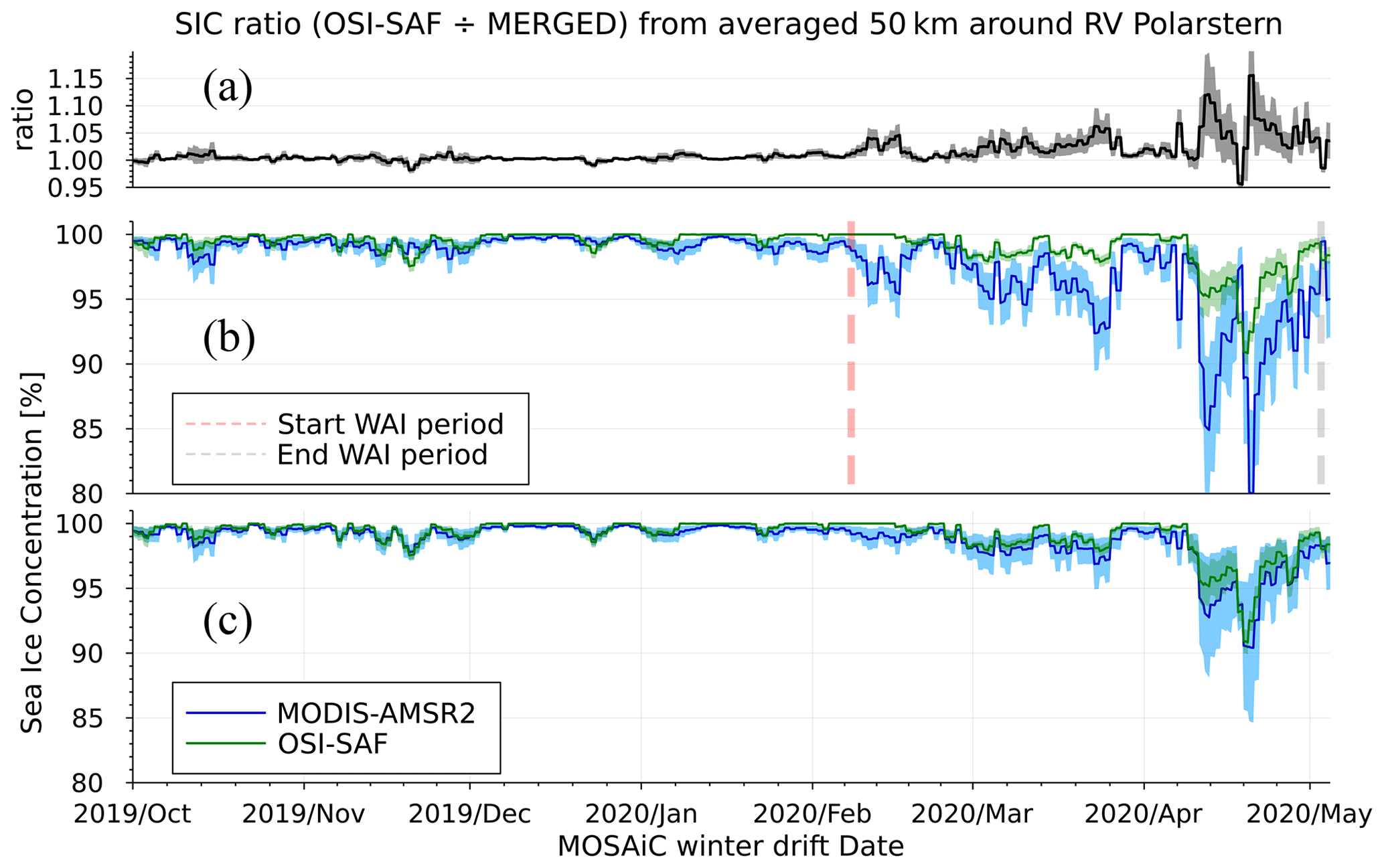
Figure C1From top to bottom: (a) the ratio of OSI SAF by MODIS–AMSR2 SIC products. A ratio close to 1 indicates that both products are on average similar within the sector of study. (b) SIC from MODIS–AMSR2 (blue) and from the OSI SAF product (green) averaged within 50 km of RV Polarstern. The initial period and end of reported warm air intrusions are marked by the dashed vertical red and grey lines. (c) The same as (b) but with the MODIS–AMSR2 SIC corrected (blue). In all panels the shaded areas correspond to 1 standard deviation.
The underestimation by MODIS–AMSR2 SIC retrievals can be observed from Fig. C1b. For the period of mid-February to the end of May 2020, considerable disagreement has been found in the SIC products obtained by the MODIS–AMSR2 and the OSI SAF retrievals. Unfortunately, the resolution of the OSI SAF product is 25 km, which is not enough to resolve small leads relevant to this study. Therefore, OSI SAF is only being used as a reference product, and we do not imply OSI SAF provides error-free retrieval or absolute values of SIC.
In Fig. D2 can be seen the advantage of detecting leads by the MODIS–AMSR2 product (Fig. D2a) as compared to the OSI SAF (Fig. D2b). Conversely OSI SAF sea ice concentration has the advantage of not being affected by the WAI events due to its different retrieval algorithm, which has been corroborated by Krumpen et al. (2021) and Rückert et al. (2023). Therefore those two products are being used in order to fix the SIC bias with OSI SAF while still keeping the high-resolution variability in the MODIS–AMSR2 product.
The time series of the OSI SAF and merged MODIS–AMSR2 products averaged over the 50 km radius around RV Polarstern is shown in Fig. C1. It clearly confirms the WAI compromised sea ice concentration mainly from February to May 2020 as reported by Rückert et al. (2023).
In order to ensure both products are statistically comparable, the MODIS–AMSR2 SIC is averaged by assuming a truncated normal distribution with 0 and 100 as lower and upper distribution limits. The averaging was performed within a 10 km grid centred on every OSI SAF coordinate grid; thus a MODIS–AMSR2 and OSI SAF dataset is achieved with the same spatial resolution as the OSI SAF grid. Then the ratio of those two products is calculated as an indicator of over- or underestimation of ASI relative to OSI SAF. The ratio is shown in Fig. C1a for the entire period of interest. It can be seen that the greatest discrepancy occurs from mid-February to May (in agreement with findings by Rückert et al., 2023) with the OSI SAF SIC retrieval being up to 15 % higher than that of MODIS–AMSR2. On the other hand the ratio rarely reaches ± 2 % for lower or higher MODIS–AMSR2 SIC outside the WAI period (mainly winter 2019), corroborating the fact that when no WAI events are experienced both products are comparable.
Since both SIC products are provided at a 24 h temporal resolution, the SIC ratio has been estimated on a daily basis. Every MODIS–AMSR2 SIC section of interest around RV Polarstern is then corrected by the SIC ratio to match on average the OSI SAF but keep the high spatial resolution and the variability within this sector of study. A comparison of this procedure is depicted in Fig. C1c, where the offset-free SIC is overlapped with the OSI SAF as a visual assessment for the feasibility of the method.
D1 Case study for 15 April 2020
Sea ice observations for 15 April 2020. In this example, both MODIS–AMSR2 (1 km resolution) and Sentinel-1 (700 m) detected the lead, whereas OSI SAF (25 km resolution) is not able to detect the lead.
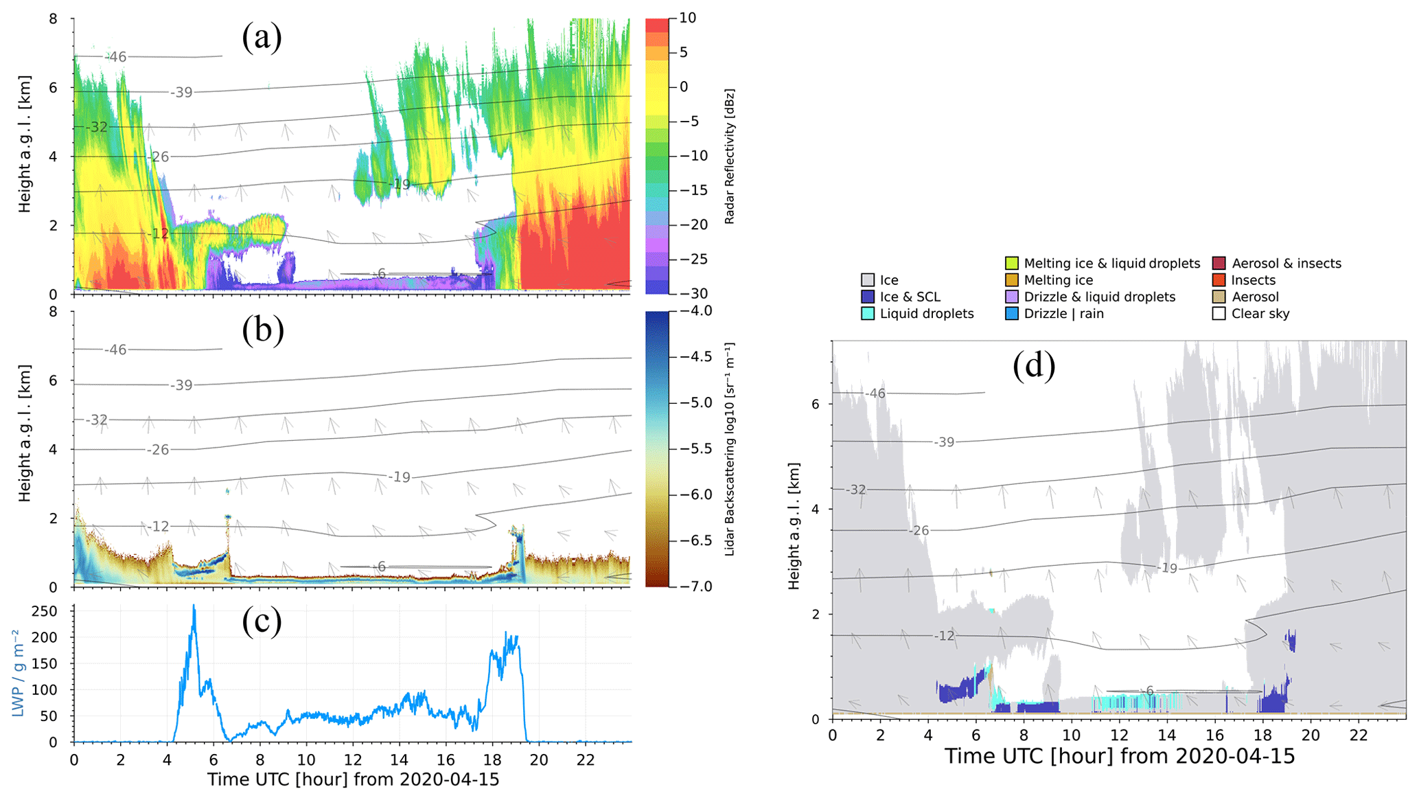
Figure D1Synergy of remote sensing instruments on board RV Polarstern for 15 April 2020. (a) KAZR cloud radar reflectivity factor; (b) PollyXT lidar backscattering coefficient; (c) liquid water path from the microwave radiometer. The isotherms and wind vectors are obtained from the weather model at selected altitudes and time steps. (d) Cloudnet classification.
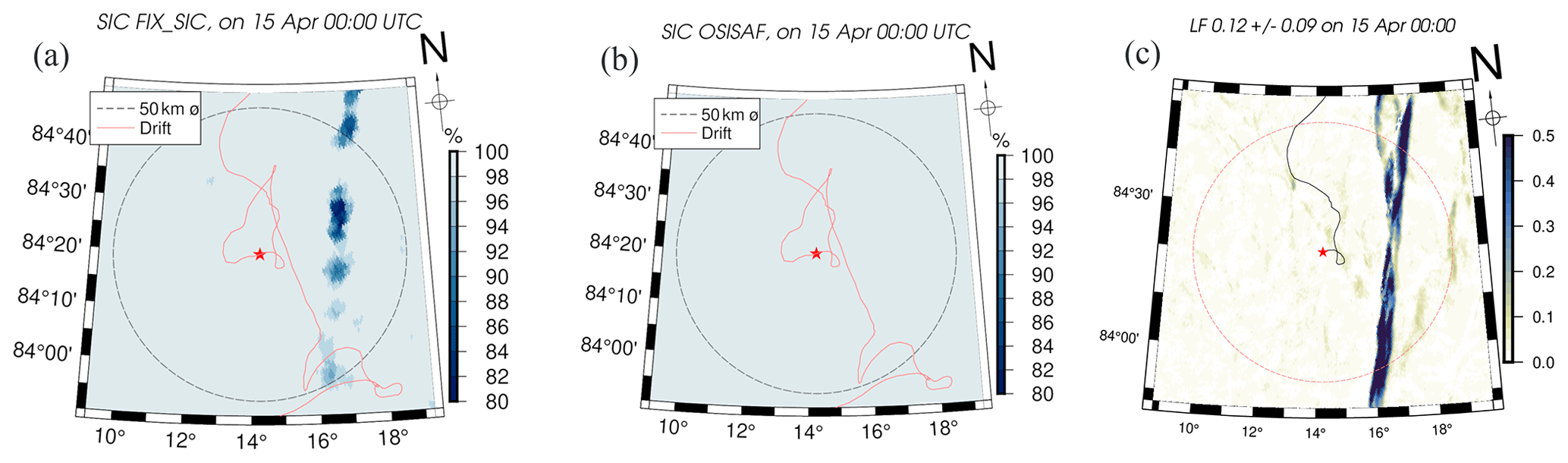
Figure D2Satellite-based sea ice observations for 15 April 2020. (a) SIC from the MODIS–AMSR2 merged product after being offset-corrected (see Appendix C). (b) SIC from OSI SAF. (c) LF from SAR Sentinel-1. The images are centred on the position of RV Polarstern (red star) on the given date. The RV drift is indicated by the red line; the dashed circle indicates the 50 km radius region of interest.
D2 Statistical analysis additional results
Figure D3a shows the frequency of occurrence of coupled-versus-decoupled cases when binned within intervals of total water path. For a total water path larger than 50 g m−2 (light- to dark-green colours), the coupled cases can be approximately 10 times more frequent than the decoupled cases (middle dashed red line), whereas cases with the total water path lower than 50 g m−2 are the most frequent observations (yellow colours) with a ratio of . It can be seen that liquid clouds are mostly found below 200 g m−2 and are more frequent than the ice clouds.
Finally the PDFs for surface skin temperature are presented in Fig. D3b, showing an asymmetric coupled–decoupled bimodal distribution. Cases with LF > 0.02 are associated with a considerable warm surface for coupled cases, with one peak located at −6 ∘C, whereas the decoupled PDF shows one peak at −17 ∘C.
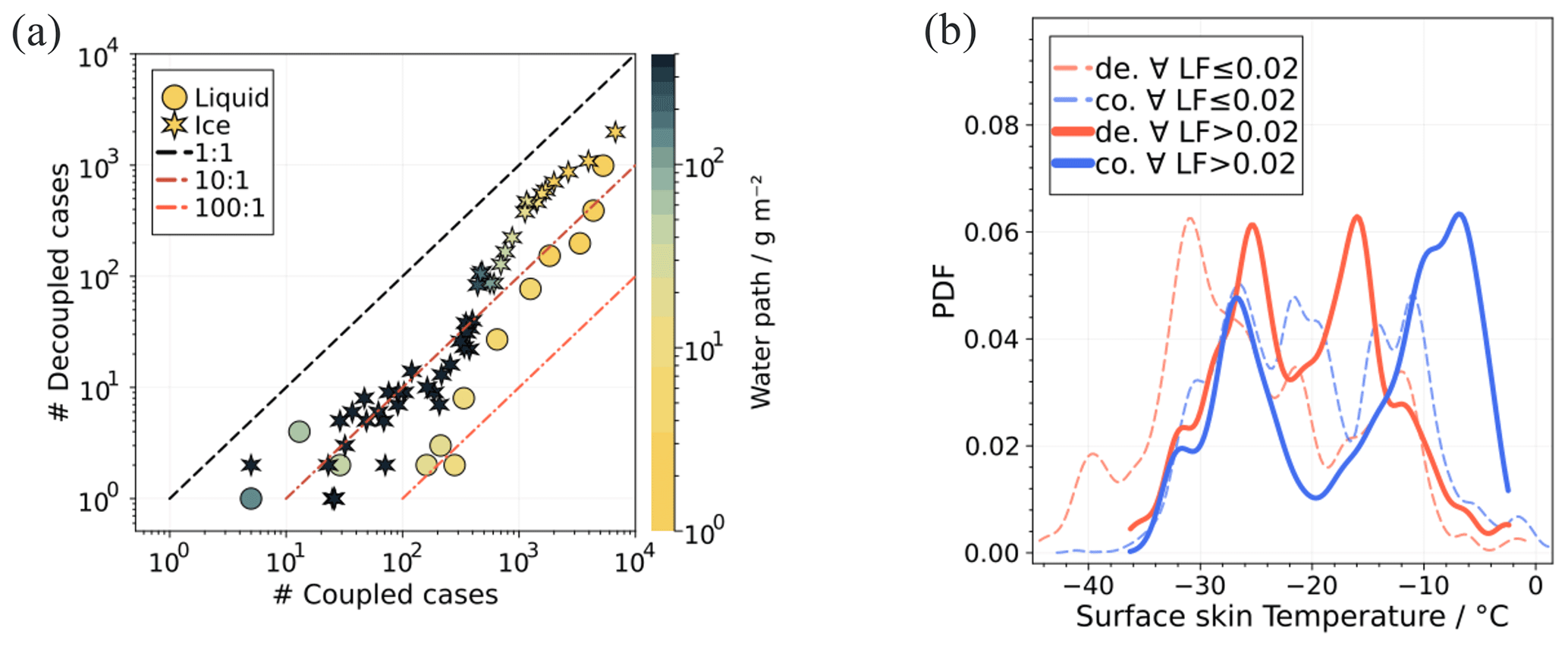
Figure D3(a) The distribution of cloud observations as a function of the integrated water path for coupled versus decoupled cases. The colour scale indicates the cloud water path for ice (stars) and liquid (circles). (b) PDF for the surface skin temperature from the GND IRT sensor.
D3 List of abbreviations and variables
| Abbreviation | Description |
| KAZR | Ka-band ARM zenith radar |
| MWR | Microwave radiometer |
| HATPRO | Humidity and Temperature Profiler |
| CEIL10m | Ceilometer 10 m resolution |
| INTERPSONDE | Interpolated Sonde |
| RV | Research vessel |
| AMSR2 | Advanced Microwave Scanning Radiometer 2 |
| MODIS | Moderate Resolution Imaging Spectroradiometer |
| MPCs | Mixed-phase clouds |
| ASI | ARTIST sea ice algorithm |
| OSI SAF | Ocean and Sea Ice Satellite Application Facility |
| SAR | Synthetic aperture radar |
| VAP | Value-added product |
Table D1Symbols, description, and corresponding units of physical quantities relevant in this study.
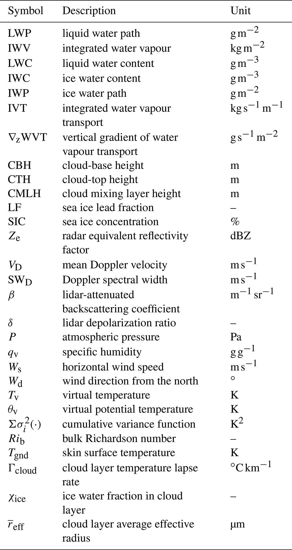
Data were obtained from the Atmospheric Radiation Measurement (ARM) user facility, a US Department of Energy (DOE) repository: https://arm.gov/data (ARM, 2023). The merged MODIS–AMSR2 1 km SIC product is publicly available at the University of Bremen data repository https://seaice.uni-bremen.de (Sea Ice Remote Sensing, 2023). HATPRO MWR data are public (https://doi.org/10.1594/PANGAEA.941389, Ebell et al., 2022). PollyXT and Cloudnet classification is available at the Cloudnet data portal under https://hdl.handle.net/21.12132/1.8865776cccd74da3 (Engelmann et al., 2023). Lead fraction data based on the divergence product from Sentinel-1 are provided following von Albedyll et al. (2023). The Cloudnet retrievals were processed using a Julia package – https://doi.org/10.5281/zenodo.7245669 (Saavedra Garfias, 2022) – and the dataset for the statistical analysis is public (https://doi.org/10.7910/DVN/DZSUV7, Saavedra Garfias and Kalesse-Los, 2023).
The supplement related to this article is available online at: https://doi.org/10.5194/acp-23-14521-2023-supplement.
PSG performed the data analysis and led the manuscript writing. HKL as project leader contributed to the research design and result analysis. LvA produced the sea ice divergence and lead fraction from SAR Sentinel-1 data. HG provided Cloudnet and the low-level cloud flag product for MOSAiC. GS provided the sea ice concentration products. All co-authors contributed with discussion and revision of the manuscript.
The contact author has declared that none of the authors has any competing interests.
Publisher's note: Copernicus Publications remains neutral with regard to jurisdictional claims made in the text, published maps, institutional affiliations, or any other geographical representation in this paper. While Copernicus Publications makes every effort to include appropriate place names, the final responsibility lies with the authors.
We thank all those who contributed to the Multidisciplinary drifting Observatory for the Study of Arctic Climate (MOSAiC) Consortium, and made this drift observatory possible (Nixdorf et al., 2021)! We express our gratitude to the DOE ARM programme for openly providing the data from its mobile facility AMF1 on board RV Polarstern. We acknowledge the open sea ice data repository from the University of Bremen and the EUMETSAT Ocean and Sea Ice Satellite Application Facility (OSI SAF). Pablo Saavedra Garfias is grateful to the project “Arctic Amplification (AC)3” for its supportive and welcome community. Thanks go to Nils Hutter, who developed the directional filter used to remove noise from the SAR divergence fields, and to Torsten Seelig for performing the Lagrangian back trajectories for the case study, as well as the three anonymous reviewers for valuable feedback and comments.
This research has been supported by the Deutsche Forschungsgemeinschaft within the Transregional Collaborative Research Center TR 172 “Arctic Amplification (AC)3” (grant no. 268020496), sub-project B07 (grant no. 437153667).
This paper was edited by Yuan Wang and reviewed by three anonymous referees.
Andreas, E. L.: Estimation of Heat and Mass Fluxes Over Arctic Leads, Mon. Weather Rev., 108, 2057–2063, https://doi.org/10.1175/1520-0493(1980)108<2057:EOHAMF>2.0.CO;2, 1980. a, b
Andreas, E. L. and Cash, B. A.: Convective heat transfer over wintertime leads and polynyas, J. Geophys. Res.-Oceans, 104, 25721–25734, https://doi.org/10.1029/1999JC900241 1999. a
ARM: Atmospheric Radiation Measurement (ARM) user facility data are collected through routine operations and scientific field experiments, US Department of Energy (DOE), https://arm.gov/data, last access: 23 November 2023. a
Bergeron, T.: On the physics of cloud and precipitation, Mémoire présenté a l'Association de Météorologie de l'U. G. G. I., Lissabon, Septembre 1933, Imprimerie Paul Dupont, Paris, 156–178, 1935. a
Chechin, D., Makhotina, I., Lüpkes, C., and Makshtas, A.: Effect of Wind Speed and Leads on Clear-Sky Cooling over Arctic Sea Ice during Polar Night, J. Atmos. Sci., 76, 2481–2503, https://doi.org/10.1175/JAS-D-18-0277.1, 2019. a
Coopman, Q., Riedi, J., Finch, D. P., and Garrett, T. J.: Evidence for Changes in Arctic Cloud Phase Due to Long-Range Pollution Transport, Geophys. Res. Lett., 45, 10709–10718, https://doi.org/10.1029/2018GL079873, 2018. a, b
Creamean, J. M., Barry, K., Hill, T. C. J., Hume, C., DeMott, P. J., Shupe, M. D., Dahlke, S., Willmes, S., Schmale, J., Beck, I., Hoppe, C. J. M., Fong, A., Chamberlain, E., Bowman, J., Scharien, R., and Persson, O.: Annual cycle observations of aerosols capable of ice formation in central Arctic clouds, Nat. Commun., 13, 3537, https://doi.org/10.1038/s41467-022-31182-x, 2022. a, b, c, d
Danker, J., Sourdeval, O., McCoy, I. L., Wood, R., and Possner, A.: Exploring relations between cloud morphology, cloud phase, and cloud radiative properties in Southern Ocean's stratocumulus clouds, Atmos. Chem. Phys., 22, 10247–10265, https://doi.org/10.5194/acp-22-10247-2022, 2022. a
Ebell, K., Walbröl, A., Engelmann, R., Griesche, H., Radenz, M., Hofer, J., and Althausen, D.: Temperature and humidity profiles, integrated water vapour and liquid water path derived from the HATPRO microwave radiometer onboard the Polarstern during the MOSAi C expedition, PANGAEA, https://doi.org/10.1594/PANGAEA.941389, 2022. a, b
Engelmann, R., Kanitz, T., Baars, H., Heese, B., Althausen, D., Skupin, A., Wandinger, U., Komppula, M., Stachlewska, I. S., Amiridis, V., Marinou, E., Mattis, I., Linné, H., and Ansmann, A.: The automated multiwavelength Raman polarization and water-vapor lidar PollyXT: the neXT generation, Atmos. Meas. Tech., 9, 1767–1784, https://doi.org/10.5194/amt-9-1767-2016, 2016. a, b
Engelmann, R., Althausen, D., Baars, H., Griesche, H., Hofer, J., Radenz, M., and Seifert, P.: Classification data from RV Polarstern on 18 November 2019, ACTRIS Cloud remote sensing data centre unit (CLU) [data set], https://hdl.handle.net/21.12132/1.8865776cccd74da3, 2023. a
Findeisen, W.: Die kolloidmeteorologischen Vorgänge bei der Niederschlagsbildung, Meteorol. Z., 55, 121–133, 1938. a
Frisch, A. S., Feingold, G., Fairall, C. W., Uttal, T., and Snider, J. B.: On cloud radar and microwave radiometer measurements of stratus cloud liquid water profiles, J. Geophys. Res.-Atmos., 103, 23195–23197, https://doi.org/10.1029/98JD01827, 1998. a
Frisch, S., Shupe, M., Djalalova, I., Feingold, G., and Poellot, M.: The Retrieval of Stratus Cloud Droplet Effective Radius with Cloud Radars, J. Atmos. Ocean. Tech., 19, 835–842, https://doi.org/10.1175/1520-0426(2002)019<0835:TROSCD>2.0.CO;2, 2002. a
Gierens, R., Kneifel, S., Shupe, M. D., Ebell, K., Maturilli, M., and Löhnert, U.: Low-level mixed-phase clouds in a complex Arctic environment, Atmos. Chem. Phys., 20, 3459–3481, https://doi.org/10.5194/acp-20-3459-2020, 2020. a, b, c
Griesche, H. J., Seifert, P., Ansmann, A., Baars, H., Barrientos Velasco, C., Bühl, J., Engelmann, R., Radenz, M., Zhenping, Y., and Macke, A.: Application of the shipborne remote sensing supersite OCEANET for profiling of Arctic aerosols and clouds during Polarstern cruise PS106, Atmos. Meas. Tech., 13, 5335–5358, https://doi.org/10.5194/amt-13-5335-2020, 2020. a, b
Griesche, H. J., Ohneiser, K., Seifert, P., Radenz, M., Engelmann, R., and Ansmann, A.: Contrasting ice formation in Arctic clouds: surface-coupled vs. surface-decoupled clouds, Atmos. Chem. Phys., 21, 10357–10374, https://doi.org/10.5194/acp-21-10357-2021, 2021. a, b
Gryschka, M., Gryanik, V. M., Lüpkes, C., Mostafa, Z., Sühring, M., Witha, B., and Raasch, S.: Turbulent Heat Exchange Over Polar Leads Revisited: A Large Eddy Simulation Study, J. Geophys. Res.-Atmos., 128, e2022JD038236, https://doi.org/10.1029/2022JD038236, 2023. a
Hogan, R. J., Mittermaier, M. P., and Illingworth, A. J.: The Retrieval of Ice Water Content from Radar Reflectivity Factor and Temperature and Its Use in Evaluating a Mesoscale Model, J. Appl. Meteorol. Clim., 45, 301–317, https://doi.org/10.1175/JAM2340.1, 2006. a, b
Howie, J. and Morris, V.: Infrared Thermometer (GNDIRT), Atmospheric Radiation Measurement (ARM) user facility [data set], https://doi.org/10.5439/1376838, 2020. a, b
Illingworth, A. J., Hogan, R. J., O'Connor, E. J., Bouniol, D., Brooks, M. E., Delanoé, J., Donovan, D. P., Eastment, J. D., Gaussiat, N., Goddard, J. W. F., Haeffelin, M., Baltink, H. K., Krasnov, O. A., Pelon, J., Piriou, J.-M., Protat, A., Russchenberg, H. W. J., Seifert, A., Tompkins, A. M., van Zadelhoff, G.-J., Vinit, F., Willén, U., Wilson, D. R., and Wrench, C. L.: CloudnetContinuous Evaluation of Cloud Profiles in Seven Operational Models Using Ground-Based Observations, B. Am. Meteorol. Soc., 88, 883–898, https://doi.org/10.1175/BAMS-88-6-883, 2007. a
Jensen, M., Giangrande, S., Fairless, T., and Zhou, A.: Interpolated Sonde (INTERPOLATEDSONDE), Atmospheric Radiation Measurement (ARM) user facility [data set], https://doi.org/10.5439/1095316, 2020. a, b
Johnson, K., Giangrande, S., and Toto, T.: Active Remote Sensing of CLouds (ARSCL) product using Ka-band ARM Zenith Radars (ARSCLKAZR1KOLLIAS), Atmospheric Radiation Measurement (ARM) user facility [data set], https://doi.org/10.5439/1393437, 2020. a
Kanitz, T., Seifert, P., Ansmann, A., Engelmann, R., Althausen, D., Casiccia, C., and Rohwer, E. G.: Contrasting the impact of aerosols at northern and southern midlatitudes on heterogeneous ice formation, Geophys. Res. Lett., 38, L17802, https://doi.org/10.1029/2011GL048532, 2011. a
Korolev, A. and Milbrandt, J.: How are mixed-phase clouds mixed?, Geophys. Res. Lett., 49, e2022GL099578, https://doi.org/10.1029/2022GL099578, 2022. a, b, c, d
Krumpen, T., von Albedyll, L., Goessling, H. F., Hendricks, S., Juhls, B., Spreen, G., Willmes, S., Belter, H. J., Dethloff, K., Haas, C., Kaleschke, L., Katlein, C., Tian-Kunze, X., Ricker, R., Rostosky, P., Rückert, J., Singha, S., and Sokolova, J.: MOSAiC drift expedition from October 2019 to July 2020: sea ice conditions from space and comparison with previous years, The Cryosphere, 15, 3897–3920, https://doi.org/10.5194/tc-15-3897-2021, 2021. a, b, c, d, e, f, g
Kwok, R.: Sea ice concentration estimates from satellite passive microwave radiometry and openings from SAR ice mo tion, Geophys. Res. Lett., 29, 25-1–25-4, https://doi.org/10.1029/2002GL014787, 2002. a, b
Lavergne, T., Tonboe, R., Lavelle, J., and Eastwood, S.: Algorithm Theoretical Basis Document (ATBD) for the OSI SAF Global Sea Ice Concentration Climate Data Record (v1.1), https://www.researchgate.net/publication/306365213_Algorithm_Theoretical_Basis_Document_ATBD_for_the_OSI_SAF_Global_Sea_Ice_Concentration_Climate_Data_Record_v11 (last access: 30 March 2023), 2016. a, b
Li, X., Krueger, S. K., Strong, C., and Mace, G. G.: Relationship Between Wintertime Leads and Low Clouds in the Pan-Arctic, J. Geophys. Res.-Atmos., 125, e2020JD032595, https://doi.org/10.1029/2020JD032595, 2020a. a
Li, X., Krueger, S. K., Strong, C., Mace, G. G., and Benson, S.: Midwinter Arctic leads form and dissipate low clouds, Nat. Commun., 11, 206, https://doi.org/10.1038/s41467-019-14074-5, 2020b. a, b
Ludwig, V., Spreen, G., and Pedersen, L. T.: Evaluation of a New Merged Sea-Ice Concentration Dataset at 1 km Resolution from Thermal Infrared and Passive Microwave Satellite Data in the Arctic, Remote Sens.-Basel, 12, 3183, https://doi.org/10.3390/rs12193183, 2020. a, b, c
Lüpkes, C., Vihma, T., Birnbaum, G., and Wacker, U.: Influence of leads in sea ice on the temperature of the atmospheric boundary layer during polar night, Geophys. Res. Lett., 35, L03805,, https://doi.org/10.1029/2007GL032461, 2008. a, b
Martin-Ralph, F., Dettinger, M., Rutz, J., and Waliser, D.: Atmospheric Rivers, Springer, https://doi.org/10.1007/978-3-030-28906-5, 2020. a, b, c
Maturilli, M., Holdridge, D. J., Dahlke, S., Graeser, J., Sommerfeld, A., Jaiser, R., Deckelmann, H., and Schulz, A.: Initial radiosonde data from 2019-10 to 2020-09 during project MOSAiC, PANGAEA, https://doi.org/10.1594/PANGAEA.928656, 2021. a
Michaelis, J. and Lüpkes, C.: The Impact of Lead Patterns on Mean Profiles of Wind, Temperature, and Turbulent Fluxes in the Atmospheric Boundary Layer over Sea Ice, Atmosphere, 13, 148, https://doi.org/10.3390/atmos13010148, 2022. a, b
Mioche, G., Jourdan, O., Ceccaldi, M., and Delanoë, J.: Variability of mixed-phase clouds in the Arctic with a focus on the Svalbard region: a study based on spaceborne active remote sensing, Atmos. Chem. Phys., 15, 2445–2461, https://doi.org/10.5194/acp-15-2445-2015, 2015. a
Morrison, H., de Boer, G., Feingold, G., Harrington, J., Shupe, M. D., and Sulia, K.: Resilience of persistent Arctic mixed-phase clouds, Nat. Geosci, 5, 11–17, https://doi.org/10.1038/ngeo1332, 2012. a, b
Murashkin, D., Spreen, G., Huntemann, M., and Dierking, W.: Method for detection of leads from Sentinel-1 SAR images, Ann. Glaciol., 59, 124–136, https://doi.org/10.1017/aog.2018.6, 2018. a
Nicolaus, M., Perovich, D. K., Spreen, G., Granskog, M. A., von Albedyll, L., Angelopoulos, M., Anhaus, P., Arndt, S., Belter, H. J., Bessonov, V., Birnbaum, G., Brauchle, J., Calmer, R., Cardellach, E., Cheng, B., Clemens-Sewall, D., Dadic, R., Damm, E., de Boer, G., Demir, O., Dethloff, K., Divine, D. V., Fong, A. A., Fons, S., Frey, M. M., Fuchs, N., Gabarró, C., Gerland, S., Goessling, H. F., Gradinger, R., Haapala, J., Haas, C., Hamilton, J., Hannula, H.-R., Hendricks, S., Herber, A., Heuzé, C., Hoppmann, M., Høyland, K. V., Huntemann, M., Hutchings, J. K., Hwang, B., Itkin, P., Jacobi, H.-W., Jaggi, M., Jutila, A., Kaleschke, L., Katlein, C., Kolabutin, N., Krampe, D., Kristensen, S. S., Krumpen, T., Kurtz, N., Lampert, A., Lange, B. A., Lei, R., Light, B., Linhardt, F., Liston, G. E., Loose, B., Macfarlane, A. R., Mahmud, M., Matero, I. O., Maus, S., Morgenstern, A., Naderpour, R., Nandan, V., Niubom, A., Oggier, M., Oppelt, N., Pätzold, F., Perron, C., Petrovsky, T., Pirazzini, R., Polashenski, C., Rabe, B., Raphael, I. A., Regnery, J., Rex, M., Ricker, R., Riemann-Campe, K., Rinke, A., Rohde, J., Salganik, E., Scharien, R. K., Schiller, M., Schneebeli, M., Semmling, M., Shimanchuk, E., Shupe, M. D., Smith, M. M., Smolyanitsky, V., Sokolov, V., Stanton, T., Stroeve, J., Thielke, L., Timofeeva, A., Tonboe, R. T., Tavri, A., Tsamados, M., Wagner, D. N., Watkins, D., Webster, M., and Wendisch, M.: Overview of the MOSAiC expedition: Snow and sea ice, Elementa, 10, 000046, https://doi.org/10.1525/elementa.2021.000046, 2022. a, b, c, d
Nixdorf, U., Dethloff, K., Rex, M., Shupe, M., Sommerfeld, A., Perovich, D. K., Nicolaus, M., Heuzé, C., Rabe, B., Loose, B., Damm, E., Gradinger, R., Fong, A., Maslowski, W., Rinke, A., Kwok, R., Spreen, G., Wendisch, M., Herber, A., Hirsekorn, M., Mohaupt, V., Frickenhaus, S., Immerz, A., Weiss-Tuider, K., König, B., Mengedoht, D., Regnery, J., Gerchow, P., Ransby, D., Krumpen, T., Morgenstern, A., Haas, C., Kanzow, T., Rack, F. R., Saitzev, V., Sokolov, V., Makarov, A., Schwarze, S., Wunderlich, T., Wurr, K., and Boetius, A.: MOSAiC Extended Acknowledgement, Zenodo, https://doi.org/10.5281/zenodo.5179739, 2021. a
Papakonstantinou-Presvelou, I., Sourdeval, O., and Quaas, J.: Strong Ocean/Sea-Ice Contrasts Observed in Satellite-Derived Ice Crystal Number Concentrations in Arctic Ice Boundary-Layer Clouds, Geophys. Res. Lett., 49, e2022GL098207, https://doi.org/10.1029/2022GL098207, 2022. a
Pruppacher, H. and Klett, J.: Microphysics of Clous and Precipitation, 2 edn., vol. 18 of Atmospheric and Oceanographic Science Library, Springer, Dordrecht, https://doi.org/10.1007/978-0-306-48100-0, 1997. a
Rogers, R. and Yau, M.: A Short Course in Clouds Physics, 3rd Edn., Pergamon Press, ISBN 9780080570945, 1991. a, b, c
Rückert, J. E., Rostosky, P., Huntemann, M., Clemens-Sewall, D., Ebell, K., Kaleschke, L., Lemmetyinen, J., Macfarlane, A. R., Naderpour, R., Stroeve, J. C., Walbröl, A., and Spreen, G.: Sea ice concentration satellite retrievals influenced by surface changes due to warm air intrusions: A case study from the MOSAiC expedition, EarthArXiv [preprint], https://eartharxiv.org/repository/view/5195/ (last access: 30 March 2023), 2023. a, b, c, d, e, f, g, h
Saavedra Garfias, P.: CloudnetTools.jl: Julia toolbox to apply Cloudnet to data from Atmospheric Radiation Measurement (ARM) facility, v1.0.0, Zenodo [code], https://doi.org/10.5281/zenodo.7245670, 2022. a
Saavedra Garfias, P.: Author Comment 2, Reply on RC2, https://doi.org/10.5194/egusphere-2023-623-AC2, 2023. a
Saavedra Garfias, P. and Kalesse-Los, H.: Wintertime Arctic cloud properties coupled to sea ice leads during MOSAiC expedition, Harvard Dataverse, https://doi.org/10.7910/DVN/DZSUV7, 2023. a
Schimmel, W., Kalesse-Los, H., Maahn, M., Vogl, T., Foth, A., Garfias, P. S., and Seifert, P.: Identifying cloud droplets beyond lidar attenuation from vertically pointing cloud radar observations using artificial neural networks, Atmos. Meas. Tech., 15, 5343–5366, https://doi.org/10.5194/amt-15-5343-2022, 2022. a
Sea Ice Remote Sensing: Sea Ice Remote Sensing at the University of Bremen, https://seaice.uni-bremen.de, last access: 23 November 2023. a
Sedlar, J., Shupe, M. D., and Tjernström, M.: On the Relationship between Thermodynamic Structure and Cloud Top, and Its Climate Significance in the Arctic, J. Climate, 25, 2374–2393, https://doi.org/10.1175/JCLI-D-11-00186.1, 2012. a
Serreze, M. C. and Barry, R. C.: Processes and impacts of Arctic amplification: A research synthesis, Global Planet. Change, 77, 85–96, https://doi.org/10.1016/j.gloplacha.2011.03.004, 2011. a
Shupe, M. D.: A ground-based multisensor cloud phase classifier, Geophys. Res. Lett., 34, L22809, https://doi.org/10.1029/2007GL031008, 2007. a
Shupe, M. D., Rex, M., Blomquist, B., Persson, P. O. G., Schmale, J., Uttal, T., Althausen, D., Angot, H., Archer, S., Bariteau, L., Beck, I., Bilberry, J., Bucci, S., Buck, C., Boyer, M., Brasseur, Z., Brooks, I. M., Calmer, R., Cassano, J., Castro, V., Chu, D., Costa, D., Cox, C. J., Creamean, J., Crewell, S., Dahlke, S., Damm, E., de Boer, G., Deckelmann, H., Dethloff, K., Dütsch, M., Ebell, K., Ehrlich, A., Ellis, J., Engelmann, R., Fong, A. A., Frey, M. M., Gallagher, M. R., Ganzeveld, L., Gradinger, R., Graeser, J., Greenamyer, V., Griesche, H., Griffiths, S., Hamilton, J., Heinemann, G., Helmig, D., Herber, A., Heuzé, C., Hofer, J., Houchens, T., Howard, D., Inoue, J., Jacobi, H.-W., Jaiser, R., Jokinen, T., Jourdan, O., Jozef, G., King, W., Kirchgaessner, A., Klingebiel, M., Krassovski, M., Krumpen, T., Lampert, A., Landing, W., Laurila, T., Lawrence, D., Lonardi, M., Loose, B., Lüpkes, C., Maahn, M., Macke, A., Maslowski, W., Marsay, C., Maturilli, M., Mech, M., Morris, S., Moser, M., Nicolaus, M., Ortega, P., Osborn, J., Pätzold, F., Perovich, D. K., Petäjä, T., Pilz, C., Pirazzini, R., Posman, K., Powers, H., Pratt, K. A., Preußer, A., Quéléver, L., Radenz, M., Rabe, B., Rinke, A., Sachs, T., Schulz, A., Siebert, H., Silva, T., Solomon, A., Sommerfeld, A., Spreen, G., Stephens, M., Stohl, A., Svensson, G., Uin, J., Viegas, J., Voigt, C., von der Gathen, P., Wehner, B., Welker, J. M., Wendisch, M., Werner, M., Xie, Z., and Yue, F.: Overview of the MOSAiC expedition–Atmosphere, Elementa, 10, 00060, https://doi.org/10.1525/elementa.2021.00060, 2022. a, b, c
Sotiropoulou, G., Sedlar, J., Tjernström, M., Shupe, M. D., Brooks, I. M., and Persson, P. O. G.: The thermodynamic structure of summer Arctic stratocumulus and the dynamic coupling to the surface, Atmos. Chem. Phys., 14, 12573–12592, https://doi.org/10.5194/acp-14-12573-2014, 2014. a
Spreen, G., Kaleschke, L., and Heygster, G.: Sea ice remote sensing using AMSR-E 89-GHz channels, J. Geophys. Res.-Oceans, 113, C02S03, https://doi.org/10.1029/2005JC003384, 2008. a
Sprenger, M. and Wernli, H.: The LAGRANTO Lagrangian analysis tool – version 2.0, Geosci. Model Dev., 8, 2569–2586, https://doi.org/10.5194/gmd-8-2569-2015, 2015. a
Tukiainen, S., O'Connor, E., and Korpinen, A.: CloudnetPy: A Python package for processing cloud remote sensing data, Journal of Open Source Software, 5, 2123, https://doi.org/10.21105/joss.02123, 2020. a
von Albedyll, L.: Sea ice deformation and sea ice thickness change, PhD thesis, Universität Bremen, https://doi.org/10.26092/elib/1868, 2022. a, b
von Albedyll, L., Haas, C., and Dierking, W.: Linking sea ice deformation to ice thickness redistribution using high-resolution satellite and airborne observations, The Cryosphere, 15, 2167–2186, https://doi.org/10.5194/tc-15-2167-2021, 2021. a
von Albedyll, L., Hendricks, S., Hutter, N., Murashkin, D., Kaleschke, L., Willmes, S., Thielke, L., Tian-Kunze, X., Spreen, G., and Haas, C.: Lead fractions from SAR-derived sea ice divergence during MOSAiC, The Cryosphere Discuss. [preprint], https://doi.org/10.5194/tc-2023-123, in review, 2023. a, b, c
Wang, D., Stachlewska, I. S., Delanoö, J., Ene, D., Song, X., and Schüttemeyer, D.: Spatio-temporal discrimination of molecular, aerosol and cloud scattering and polarization using a combination of a Raman lidar, Doppler cloud radar and microwave radiometer, Opt. Express, 28, 20117–20134, https://doi.org/10.1364/OE.393625, 2020. a
Wegener, A.: Thermodynamik der atmosphäre, Verlag von Johann Ambrosius Barth, Leipzig, https://doi.org/10.1002/qj.49703916510, pp. 8+331, 1911. a
Wendisch, M., Brückner, M., Burrows, J. P., Crewell, S., Dethloff, K., Ebell, K., Lüpkes, C., Macke, A., Notholt, J., Quaas, J., Rinke, A., and Tegen, I.: Understanding causes and effects of rapid warming in the Arctic, Eos, 98, 22–26, https://doi.org/10.1029/2017EO064803, 2017. a
Wendisch, M., Brückner, M., Crewell, S., Ehrlich, A., Notholt, J., Lüpkes, C., Macke, A., Burrows, J. P., Rinke, A., Quaas, J., Maturilli, M., Schemann, V., Shupe, M. D., Akansu, E. F., Barrientos-Velasco, C., Bärfuss, K., Blechschmidt, A.-M., Block, K., Bougoudis, I., Bozem, H., Böckmann, C., Bracher, A., Bresson, H., Bretschneider, L., Buschmann, M., Chechin, D. G., Chylik, J., Dahlke, S., Deneke, H., Dethloff, K., Donth, T., Dorn, W., Dupuy, R., Ebell, K., Egerer, U., Engelmann, R., Eppers, O., Gerdes, R., Gierens, R., Gorodetskaya, I. V., Gottschalk, M., Griesche, H., Gryanik, V. M., Handorf, D., Harm-Altstädter, B., Hartmann, J., Hartmann, M., Heinold, B., Herber, A., Herrmann, H., Heygster, G., Höschel, I., Hofmann, Z., Hölemann, J., Hünerbein, A., Jafariserajehlou, S., Jäkel, E., Jacobi, C., Janout, M., Jansen, F., Jourdan, O., Jurányi, Z., Kalesse-Los, H., Kanzow, T., Käthner, R., Kliesch, L. L., Klingebiel, M., Knudsen, E. M., Kovács, T., Körtke, W., Krampe, D., Kretzschmar, J., Kreyling, D., Kulla, B., Kunkel, D., Lampert, A., Lauer, M., Lelli, L., von Lerber, A., Linke, O., Löhnert, U., Lonardi, M., Losa, S. N., Losch, M., Maahn, M., Mech, M., Mei, L., Mertes, S., Metzner, E., Mewes, D., Michaelis, J., Mioche, G., Moser, M., Nakoudi, K., Neggers, R., Neuber, R., Nomokonova, T., Oelker, J., Papakonstantinou-Presvelou, I., Pätzold, F., Pefanis, V., Pohl, C., van Pinxteren, M., Radovan, A., Rhein, M., Rex, M., Richter, A., Risse, N., Ritter, C., Rostosky, P., Rozanov, V. V., Donoso, E. R., Saavedra Garfias, P., Salzmann, M., Schacht, J., Schäfer, M., Schneider, J., Schnierstein, N., Seifert, P., Seo, S., Siebert, H., Soppa, M. A., Spreen, G., Stachlewska, I. S., Stapf, J., Stratmann, F., Tegen, I., Viceto, C., Voigt, C., Vountas, M., Walbröl, A., Walter, M., Wehner, B., Wex, H., Willmes, S., Zanatta, M., and Zeppenfeld, S.: Atmospheric and Surface Processes, and Feedback Mechanisms Determining Arctic Amplification: A Review of First Results and Prospects of the (AC)3 Project, B. Am. Meteorol. Soc., 104, E208–E242, https://doi.org/10.1175/BAMS-D-21-0218.1, 2023. a
Westbrook, C. D. and Illingworth, A. J.: Evidence that ice forms primarily in supercooled liquid clouds at temperatures > −27 ∘C, Geophys. Res. Lett., 38, L14808, https://doi.org/10.1029/2011GL048021, 2011. a, b
Zhang, D., Morris, V., and Ermold, B.: Ceilometer (CEIL10m), Atmospheric Radiation Measurement (ARM) user facility [data set], 2020. a
Zhu, Y. and Newell, R. E.: A Proposed Algorithm for Moisture Fluxes from Atmospheric Rivers, Mon. Weather Rev., 126, 725–735, https://doi.org/10.1175/1520-0493(1998)126<0725:APAFMF>2.0.CO;2, 1998. a, b
- Abstract
- Introduction
- Instrumentation and data products
- Methodology
- Results
- Discussion and conclusions
- Appendix A: Cloud decoupling criteria
- Appendix B: Derivation for the gradient of water vapour transport
- Appendix C: Sea ice concentration offset correction
- Appendix D: Supporting material
- Code and data availability
- Author contributions
- Competing interests
- Disclaimer
- Acknowledgements
- Financial support
- Review statement
- References
- Supplement