the Creative Commons Attribution 4.0 License.
the Creative Commons Attribution 4.0 License.
 | 22 Nov 2023
Quantification of fossil fuel CO2 from combined CO, δ13CO2 and Δ14CO2 observations
Jinsol Kim
John B. Miller
Charles E. Miller
Scott J. Lehman
Sylvia E. Michel
Vineet Yadav
Nick E. Rollins
William M. Berelson
We present a new method for partitioning observed CO2 enhancements (CO2xs) into fossil and biospheric fractions (Cff and Cbio) based on measurements of CO and δ13CO2, complemented by flask-based Δ14CO2 measurements. This method additionally partitions the fossil fraction into natural gas and petroleum fractions (when coal combustion is insignificant). Although here we apply the method only to discrete flask air measurements, the advantage of this method (CO- and δ13CO2-based method) is that CO2xs partitioning can be applied at high frequency when continuous measurements of CO and δ13CO2 are available. High-frequency partitioning of CO2xs into Cff and Cbio has already been demonstrated using continuous measurements of CO (CO-based method) and Δ14CO2 measurements from flask air samples. We find that the uncertainty in Cff estimated from the CO- and δ13CO2-based method averages 3.2 ppm (23 % of the mean Cff of 14.2 ppm estimated directly from Δ14CO2), which is significantly less than the CO-based method which has an average uncertainty of 4.8 ppm (34 % of the mean Cff). Using measurements of CO, δ13CO2 and Δ14CO2 from flask air samples at three sites in the greater Los Angeles (LA) region, we find large contributions of biogenic sources that vary by season. On a monthly average, the biogenic signal accounts for −14 to +25 % of CO2xs with larger and positive contributions in winter and smaller and negative contributions in summer due to net respiration and net photosynthesis, respectively. Partitioning Cff into petroleum and natural gas combustion fractions reveals that the largest contribution of natural gas combustion generally occurs in summer, which is likely related to increased electricity generation in LA power plants for air-conditioning.
- Article
(3923 KB) - Full-text XML
-
Supplement
(565 KB) - BibTeX
- EndNote


The world's cities account for up to 70 % of global greenhouse gas (GHG) emissions, while covering less than 2 % of the Earth's surface (IPCC, 2014). Cities around the world have started implementing mitigation strategies to reduce carbon dioxide (CO2) emissions and collaborate with each other in organizations such as the C40 Cities Climate Leadership Group (https://www.c40.org/, last access: 25 October 2023) and the Global Covenant of Mayors for Climate & Energy (https://www.globalcovenantofmayors.org/, last access: 25 October 2023). To support urban efforts, monitoring systems are necessary to evaluate and verify reductions attributable to specific mitigation strategies (Turnbull et al., 2022).
Current understanding of anthropogenic CO2 emissions mainly derives from methods that estimate aggregate emissions in a domain using economic statistics such as total fuel sales or activity data such as total distance traveled for on-road vehicle emissions. These “bottom-up” methods provide specific location and process information that relies on mapping the source-specific emission factors and measurements of activities (e.g., McDonald et al., 2014; Gurney et al., 2019; Gately and Hutyra, 2017; Super et al., 2020). In contrast, more recently “top-down” methods that quantify emissions from measurements of atmospheric CO2 have been used to estimate emissions. These top-down approaches typically use either a mass balance technique where an initial estimate is not required (e.g., Mays et al., 2009; Cambaliza et al., 2014; Heimburger et al., 2017; Ahn et al., 2020) or an inverse/data assimilation approach where observations and a prior map of emissions are combined to generate a best estimate (e.g., Bréon et al., 2015; Staufer et al., 2016; Sargents et al., 2018; Turner et al., 2020; Lauvaux et al., 2016, 2020).
To estimate anthropogenic CO2 emissions using top-down methods, it is crucial to separate the fossil fuel signals from the biogenic signals, which can vary from negative (uptake) to positive (emission) across the annual cycle. Recent analyses of urban CO2 suggest that biogenic emissions and uptake have significant magnitudes relative to fossil fuel fluxes, especially during the growing season (Sargent et al., 2018; Vogel et al., 2019; Miller et al., 2020). Previous top-down studies have used biosphere models to estimate biogenic fluxes and have then focused on determining the balance of emissions attributable to fossil fuel combustion assuming that the biogenic emissions are known (Sargent et al., 2018; Turner et al., 2020; Lauvaux et al., 2020). However, even with recent improvements in biosphere models (Wu et al., 2021; Gourdji et al., 2022) the actual magnitude and variability of these fluxes are still not well constrained (Hardiman et al., 2017; Winbourne et al., 2022), potentially leading to unknown observational bias in the associated estimates of fossil-fuel-derived emissions.
Radiocarbon (14CO2) provides the ability to separate biogenic and anthropogenic CO2 fluxes and mole fractions from an observational point of view (e.g., Levin et al., 2003; Turnbull et al., 2006). Observational methods rely on the fact that fossil fuels and the resultant CO2 produced during combustion are completely devoid of 14C (i.e., Δ14C ‰ on the widely used delta scale; Stuiver and Polach, 1977). Measurements of Δ14CO2, acquired at timescales of weeks to months allow quantification of seasonal variations in biogenic and fossil contributions to the atmospheric CO2 mole fraction (e.g., Djuricin et al., 2010; Miller et al., 2012; Turnbull et al., 2015). 14C methods typically require air sample collection, preparation and analysis via accelerator mass spectrometry, which limits the number of measurements, although a number of promising optical methods for in situ 14CO2 measurement at natural abundance are currently being developed (Fleisher et al., 2017; Genoud et al., 2019; McCartt and Jiang, 2022).
On the other hand, carbon monoxide (CO) is a widely used tracer that can be measured continuously in situ using high-precision optical analyzers (e.g., Vogel et al., 2010; Newman et al., 2013; Turnbull et al., 2015; Lauvaux et al., 2020). CO is often co-emitted with fossil fuel CO2 (CO2ff) during incomplete combustion. If the COxs:CO2ff ratio (Rff, where COxs is the CO enhancement above the background) is well constrained, continuous CO measurements combined with Rff can provide an estimate of continuous CO2ff. A few studies have applied this method to estimate fossil fuel emissions for a moment in time during an airborne measurement campaign (Graven et al., 2009; Turnbull et al., 2011). However, with this approach it is challenging to identify interannual trends because Rff at a site may vary significantly on timescales ranging from hours to years (Levin and Karstens, 2007; Vogel et al., 2010). The CO:CO2 emission ratio can vary by sources depending on the carbon content of the fuel and combustion conditions. Due to the impacts of atmospheric transport at a given observation site and the variability in the source combination in time and space, Rff also varies in time and space. Additionally, CO produced from oxidation of volatile organic compounds (VOCs) can have an effect (Vimont et al., 2019).
Vardag et al. (2015) proposed dividing fossil fuel emissions further into two groups that may display less variability in the CO:CO2 emission ratio. If one group is well constrained by CO and the other by 13CO2, each group can be identified by combining CO and 13CO2 observations. Vardag et al. (2015) focused on separating traffic from non-traffic emissions or biofuel emissions from the other fossil fuel emissions. However, no significant benefit of combining CO and 13CO2 was found because traffic and biofuel CO2 do not produce a distinct CO:CO2 emission ratio or 13CO2 isotopic signatures compared to the other CO2ff source terms.
Here, we differentiate CO2 signals from biogenic, petroleum and natural gas sources by combining CO, δ13CO2 and Δ14CO2 measurements. The combination of Δ14CO2 and δ13CO2 has been used previously to distinguish biogenic, petroleum and natural gas signals for air sampling events (Lopez et al., 2013; Djuricin et al., 2010) and at a seasonal scale (Newman et al., 2016). In contrast, the combination of CO and δ13CO2, which can both be measured at high frequency, enables source partitioning at higher temporal resolution. We demonstrate the agreement between the existing Δ14CO2 and δ13CO2 and newly proposed CO and δ13CO2 methods. This establishes the utility of the CO and δ13CO2 method in partitioning CO2xs into fossil fuel and biogenic components, with further partitioning of fossil fuel sources into petroleum and natural gas sources, in the megacity of Los Angeles (LA).
Here, we describe two methods for separating fossil fuel and biogenic components from atmospheric CO2 measurements in the complex urban environment of the megacity of Los Angeles (LA). Section 2.2 describes our application of the method already described by Newman et al. (2016) using Δ14CO2 and δ13CO2 observations. The details of the new method utilizing CO and δ13CO2 measurements are described in Sect. 2.3. Briefly, we take advantage of the fact that the combination of the CO:CO2 emission ratio and the 13CO2 isotopic signature reveals a very distinct pattern for biogenic, petroleum and natural gas sources. However, this approach requires knowledge of the CO:CO2 emission ratio and the isotopic signature of each source. We apply isotopic signatures reported by previous studies, and CO:CO2 emission ratios are determined for LA using measurements of CO, δ13CO2 and Δ14CO2 from flask samples. Flask measurements are described in Sect. 2.1, and the source apportionment from Δ14CO2 and δ13CO2 observations, which is used to derive CO:CO2 emission ratios for each source, is described in Sect. 2.2.
2.1 Measurements
We use measurements from air samples collected at 14:00 local standard time at three existing Los Angeles Megacity Carbon Project sites: the University of Southern California (USC); California State University, Fullerton (FUL); and Granada Hills (GRA) (Miller et al., 2020). Air samples were collected from November 2014 to March 2016 using the National Oceanic and Atmospheric Administration (NOAA) programmable flask packages (PFPs) and programmable compressor packages (Sweeney et al., 2015). The samples were sent back to the NOAA Global Monitoring Laboratory where greenhouse gases including CO2 as well as CO mole fractions were measured using NOAA's high-precision/high-accuracy greenhouse gas measurement system (Sweeney et al., 2015). After the measurement, residual air is extracted from PFP flasks, and CO2 is isolated for 14C measurement using established cryogenic and mass spectrometric techniques (Lehman et al., 2013). Samples are purified, graphitized and packed into individual targets at the University of Colorado, Boulder, Institute of Arctic and Alpine Research (INSTAAR), and then sent to the University of California, Irvine, Keck Carbon Cycle Accelerator Mass Spectrometer Facility, for high-precision Δ14C measurement. 1σ measurement uncertainty is ∼1.8 ‰, equivalent to ∼ 1.2 parts per million (ppm) of recently added fossil fuel CO2. δ13CO2 in PFP samples is measured by dual-inlet isotope ratio mass spectrometry with a precision of approximately 0.02 ‰ at the INSTAAR Stable Isotope Laboratory (Vaughn et al., 2004; Sweeney et al., 2015).
Enhancement of each species is defined relative to a time-dependent background level, which is based on nighttime (02:00 local standard time) measurements made at Mount Wilson Observatory (MWO; Fig. 1) located at 1670 m above sea level. Nighttime air at MWO generally represents the relatively clean, well-mixed free troposphere since polluted LA Basin boundary layer air has typically descended back into the basin by this time. After an additional step of filtering obvious outliers corresponding to pollution events indicated by anomalously elevated concentrations, values were interpolated to the time of observations within the LA Basin by fitting curves to the screened MWO data (Fig. 2). A further analysis of associated CO measurements indicates that background reconstructed using nighttime air samples from MWO is representative of clean background air coming from either onshore or offshore (Miller et al., 2020).
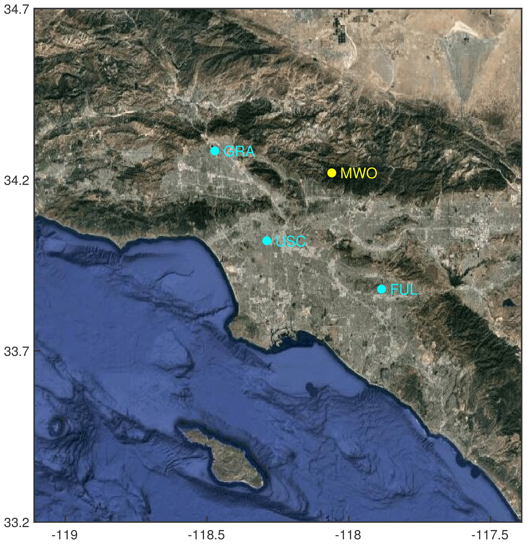
Figure 1Map of the greater Los Angeles region. The three Los Angeles Megacity Carbon Project sites are marked in cyan, and the Mount Wilson Observatory used to define background values is marked in yellow. Map data © Google Maps 2022.
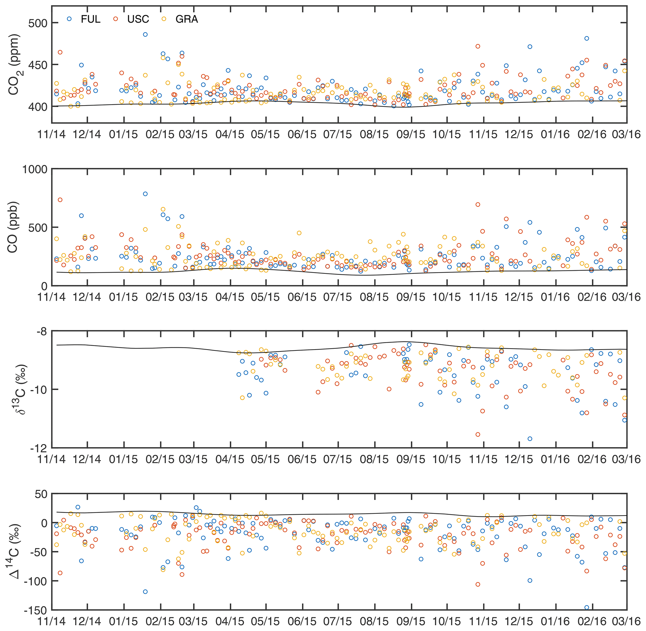
Figure 2Time series of CO2, CO, δ13C and Δ14C. The black line represents background values. The dates are labeled as month/year.
2.2 Partitioning CO2 signals using flask-based Δ14CO2 and δ13CO2 measurements
Our general approach to distinguishing CO2 signals from biogenic, petroleum and natural gas sources using Δ14CO2 and δ13CO2 follows the procedure described by Newman et al. (2016). Following previous derivations (e.g., Turnbull et al., 2006; Miller et al., 2020), we start with the definition for CO2ff, which is based on mass balances for the atmospherically conserved quantities Δ14C × CO2 and CO2:
Measured CO2 mole fractions and Δ14C values are abbreviated as C and Δ. The subscripts obs, bkg, ff and r represent observations, background, fossil fuel and respiration, respectively. Δff is equal to −1000 ‰. As in the Miller et al. (2020) study focusing on LA, we estimate the value of the small respiratory term, , as 0.25 ppm. The overall uncertainty in Cff for LA measurements during 2015 is approximately 1.2 ppm, which includes 100 % uncertainty assigned to the respiratory term. Cff and Cbio (Cbio=Cxs–Cff) are calculated for all available flask air samples during the 2014–2016 sampling period, at a frequency of approximately 3 times per week at each of the three sites.
Cff is then separated into signals from petroleum and natural gas combustion using 13C:12C ratios (δ13C as defined by standard isotopic definition; Craig, 1957) measured on the same air samples. First, the flux weighted-mean δ13C signature of all sources located in the observation footprints (δsrc) is determined on a sample-by-sample basis using the combined mass balances for δ13C × CO2 and CO2:
where δ is shorthand for δ13CO2. The uncertainties in Cobs, Cbkg, δobs and δbkg are 0.1 ppm, 1.5 ppm, 0.02 ‰ and 0.08 ‰, respectively. The obs uncertainties are measurement uncertainties, while the bkg uncertainties are determined as the standard deviation of the difference between the observations and their smoothed-curve representation at MWO. The median uncertainty in δsrc is 3.0 ‰ and is calculated by propagating the uncertainties listed above, including covariance between δ13C and δ13C × CO2.
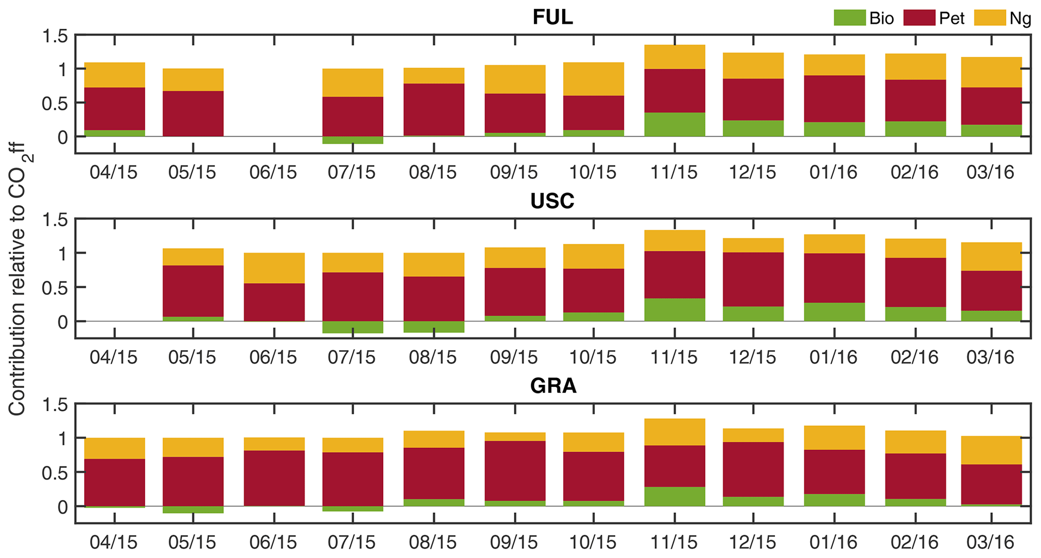
Figure 3Monthly mean fractional contributions (f) of biosphere (green), petroleum (red) and natural gas (yellow) to CO2xs at each site, as determined from Δ14C and δ13C observations (Sect. 2.2). The sum of the fractions is 1 in each month. The dates are labeled as month/year.
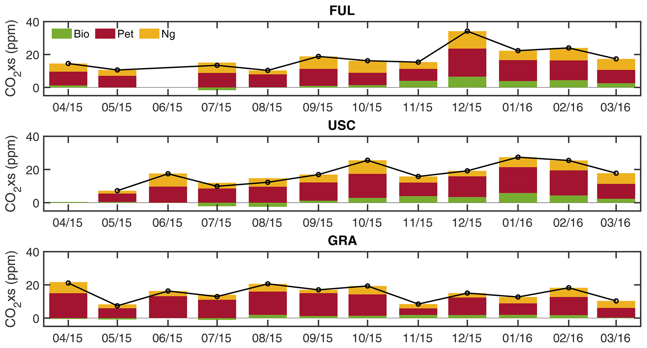
Figure 4Monthly mean CO2xs partitioned into biosphere (green), petroleum (red) and natural gas (yellow) signals, as determined from Δ14C and δ13C observations, at each site. The black marker indicates CO2xs. The dates are labeled as month/year.
We combine Cff (Eq. 1) and δsrc (Eq. 2) to determine the δ13C signature of fossil fuel emissions, δff:
Rearranging yields
where f is the fraction. Following Newman et al. (2016), we take the isotopic signature of biospheric CO2 fluxes (δbio) to be ‰ based on the analysis of Northern Hemisphere mid-latitude CO2 and δ13C observations (Bakwin et al., 1998b), which reflects the predominance of C3 photosynthesis. However, because LA turfgrasses, which could account for a significant fraction of urban CO2 fluxes (Miller, 2020), are often C4 species (e.g., Bermuda and Buffalo grasses), we also conduct tests using ‰, representing a C3–C4 mix (Fig. S1). When we change δbio from −26.6 ‰ to −20 ‰, fpet decreases by 0.04, and fng increases by 0.05, which is smaller than the median uncertainty in fpet and fng, which is 0.17 and 0.16, respectively. fff is the fraction of Cff in Cxs, i.e., , and . Lastly, the proportions of Cff emitted by petroleum (pet) and natural gas (ng) combustion, fpet and fng, are calculated from the values of δff:
We use values of ‰ for δpet (Newman et al., 2016; measurements in 2014) and ‰ for δng (Newman et al., 2008); , and , where . We use temporally constant δ13C signatures for petroleum, natural gas and biogenic sources (and sinks), although with additional processed-based information, this assumption could be relaxed in the future. Note that although pet, ng and bio signatures are fixed, both δsrc and δff vary with time, meaning that fbio, fpet and fng all vary at the frequency of the air sampling. Samples with calculated values outside the range of 0 and 1, corresponding to small CO2xs and large uncertainty in δsrc, are excluded from the analysis.
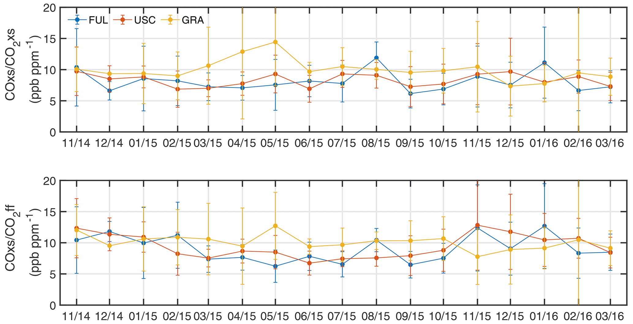
Figure 5Monthly variations in (Rsrc) and (Rff) at each site. is calculated using 14C observations. The dates are labeled as month/year.
2.3 Partitioning CO2 signals using CO and δ13CO2 measurements
Although we can determine fbio, fpet and fng at the frequency of discrete flask sampling events using the method described in Sect. 2.2, here we describe how comparable CO2xs fractions can in theory be determined at high frequency using continuous measurements of CO and δ13CO2. To evaluate the method, we compute the relative contributions of biogenic, petroleum and natural gas sources to CO2xs using flask air CO and δ13CO2 measurements and compare these to values obtained using the Δ14CO2-guided approach for the same samples by applying the following system of equations:
Rsrc represents the ratio of the total source, which is the observed ratio, and we use R to refer to the emission ratios of individual CO2xs components (bio, pet and ng). For now, we assume that R of each source is constant over a year-long period and over the greater LA region (discussed in Sect. 3.2); especially with high-frequency CO and δ13CO2 measurements, this assumption could easily be relaxed (discussed in Sect. 3.3).
R values and δ13C signatures for bio, pet and ng are needed to solve Eqs. (7)–(9). δ13C signatures are specified in Sect. 2.2; R values are obtained via multiple linear regression of Eq. (7) using observed Rsrc and f values determined using Δ14C and δ13C of CO2 measurements as described in Sect. 2.2. Then we solve Eqs. (7)–(9) for new f values, f′. This new CO2xs partitioning (i.e., , , based on CO and δ13CO2 observations is used to calculate new values of Cff and Cbio (i.e., and .
3.1 Contribution of biogenic, petroleum and natural gas sources to CO2 excess
We calculated the fractional contribution of petroleum, natural gas and biospheric fluxes to total CO2xs each month from April 2015 to March 2016 using Δ14CO2 and δ13CO2 observations recorded at FUL, USC and GRA. The results are given in Table S1 and presented in Fig. 3. Figure 4 presents the results in terms of the relative CO2xs contribution from each source at each site. We observe seasonal variation in CO2xs from each source. Fossil fuel is the dominant CO2 emissions source at each site, which agrees with the findings of Newman et al. (2016) and Miller et al. (2020). Annually averaged across all three sites, biogenic emissions account for 6 % of CO2xs. Biogenic emissions are larger and positive in winter and smaller and negative in summer, indicating winter respiration and uptake in summertime, generally consistent with the results of Miller et al. (2020). Note that in this study, we do not partition Cbio into an urban biosphere component and other components. Other components include the oxidation of biogenic carbon including ethanol added to gasoline, and human and other animal food and waste (which can only be positive and are unlikely to vary much seasonally). If, as in Miller et al. (2020), we accounted for the always positive ethanol, food and waste signals, we would likely observe similarly large seasonal drawdown associated with urban vegetation.
Table 1Bottom-up CO2 emission, CO emission and R ( ratio) estimates for each source sector and fuel type for the LA Basin based on the Vulcan 3.0 and the US Environmental Protection Agency (EPA) National Emission Inventory for the 2011 (NEI 2011) product. NEI 2011 is scaled by the emissions with a fuel consumption dataset from the US Energy Information Administration (EIA) State Energy Data System (SEDS) to estimate 2015 CO emissions.
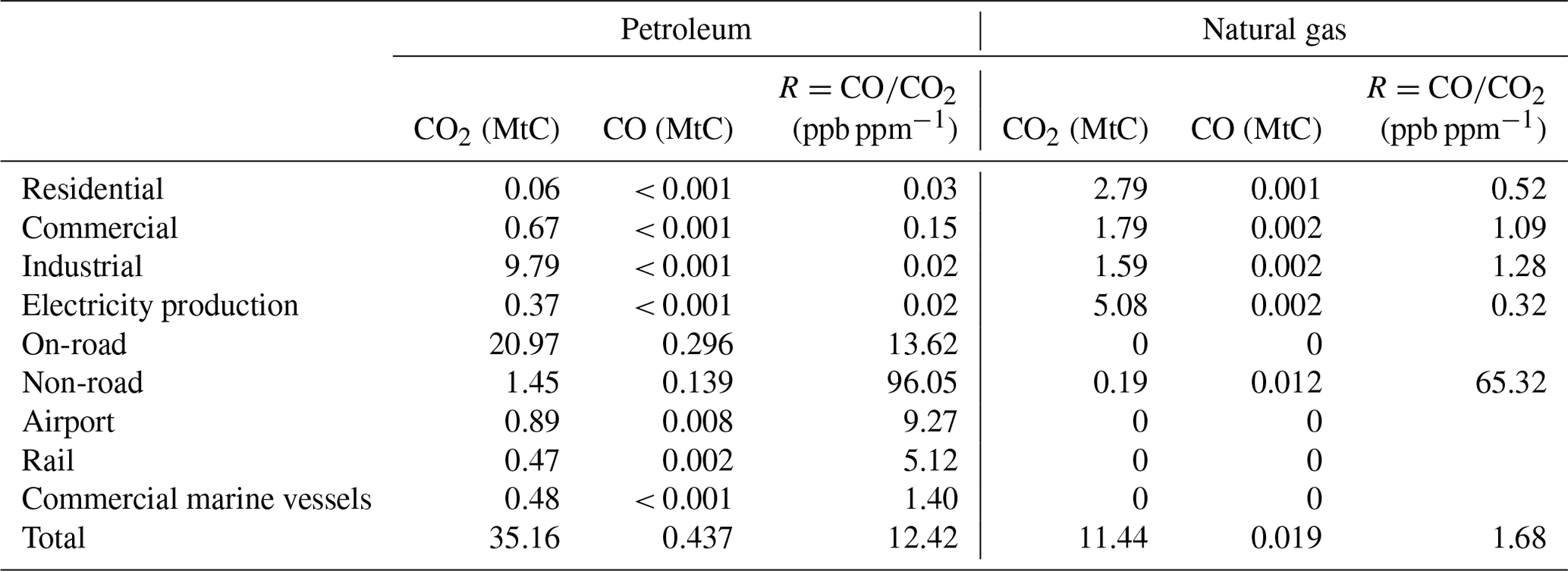
Table 2 ratios (R) and δ13C signatures used to determine the relative contribution of biogenic, petroleum and natural gas sources.
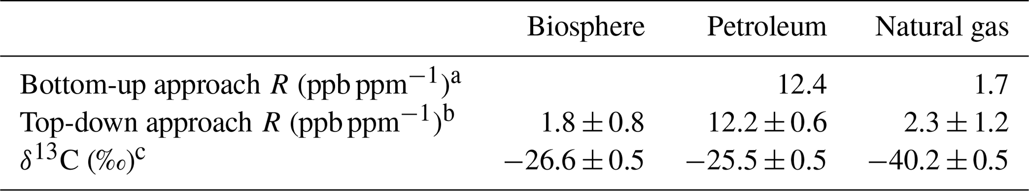
a R calculated from Table 1. These values are not used for CO2xs partitioning and are for reference only.
b R calculated from CO, δ13CO2 and Δ14CO2 flask observations. These values are used in this study.
c δ13C from previous studies (Bakwin et al., 1998a; Newman et al., 2008).
We also observe spatial differences: the USC site exhibits a smaller contribution of the biosphere (3 % of annual average CO2 excess) compared to FUL and GRA (9 % and 5 % of total CO2 excess, respectively). However, these modest annual average biospheric contributions mask significant seasonal activity. On a monthly basis, maximum positive biogenic contribution is observed in November at 25 %, 26 % and 22 % at USC, FUL and GRA (percentage of total CO2 excess, respectively). And the maximum negative contribution, driven by net photosynthesis, is observed in July with values of −22 %, −13 % and −12 % at USC, FUL and GRA (percentage of total CO2 excess, respectively).
The network average Cff is 11.0 ± 14.5 ppm in winter (November–February; median and standard deviation) and 12.2 ± 6.6 ppm in summer (May–August). No significant difference is observed in winter and summer Cff. This corresponds to the seasonality in Hestia-LA emissions, which indicates Cff inputs are only 3 % higher in winter. High variability observed in wintertime Cff agrees with Miller et al. (2020), which is likely caused by increased temperature inversion trapping as the cold ground surface in winter cools the air layer right above the ground. While Hestia-LA estimated the relative contribution of petroleum and natural gas to fossil fuel emissions as 75 % and 25 %, we observe a lower contribution of petroleum, 67 %, and a larger contribution of natural gas, 33 %. Furthermore, the top-down seasonality of petroleum and natural gas (Fig. 4), which as fractions of Cff should be largely independent of mixing, is clearly evident. The proportions of natural gas in fossil fuel signals are 40 % and 36 % in summer and 34 % and 30% in winter at FUL and USC (Fig. 3). The increase in the natural gas contribution observed in summer can be explained by the increase in natural-gas-generated electricity in LA power plants to provide for air-conditioning in summer (Newman et al., 2016; He et al., 2019) as well as the air dominantly blowing from the southwest during summer. GRA, located northwest of USC by ∼ 35 km without an electricity generation facility nearby, shows the opposite pattern (24 % in summer and 40 % in winter). This suggests the local influence of increased natural gas usage for heating in the winter.
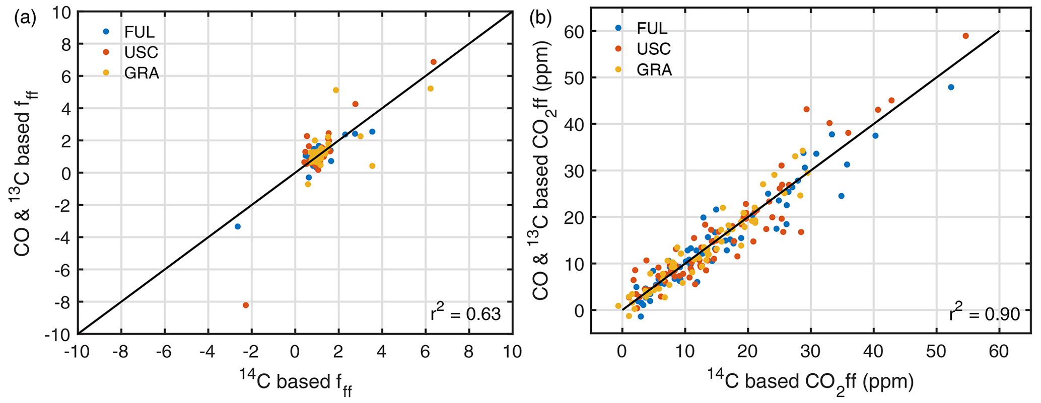
Figure 6Comparison of fff and (a) and Cff and (b). The black lines represent 1:1 relationships, and different colors indicate different sites.
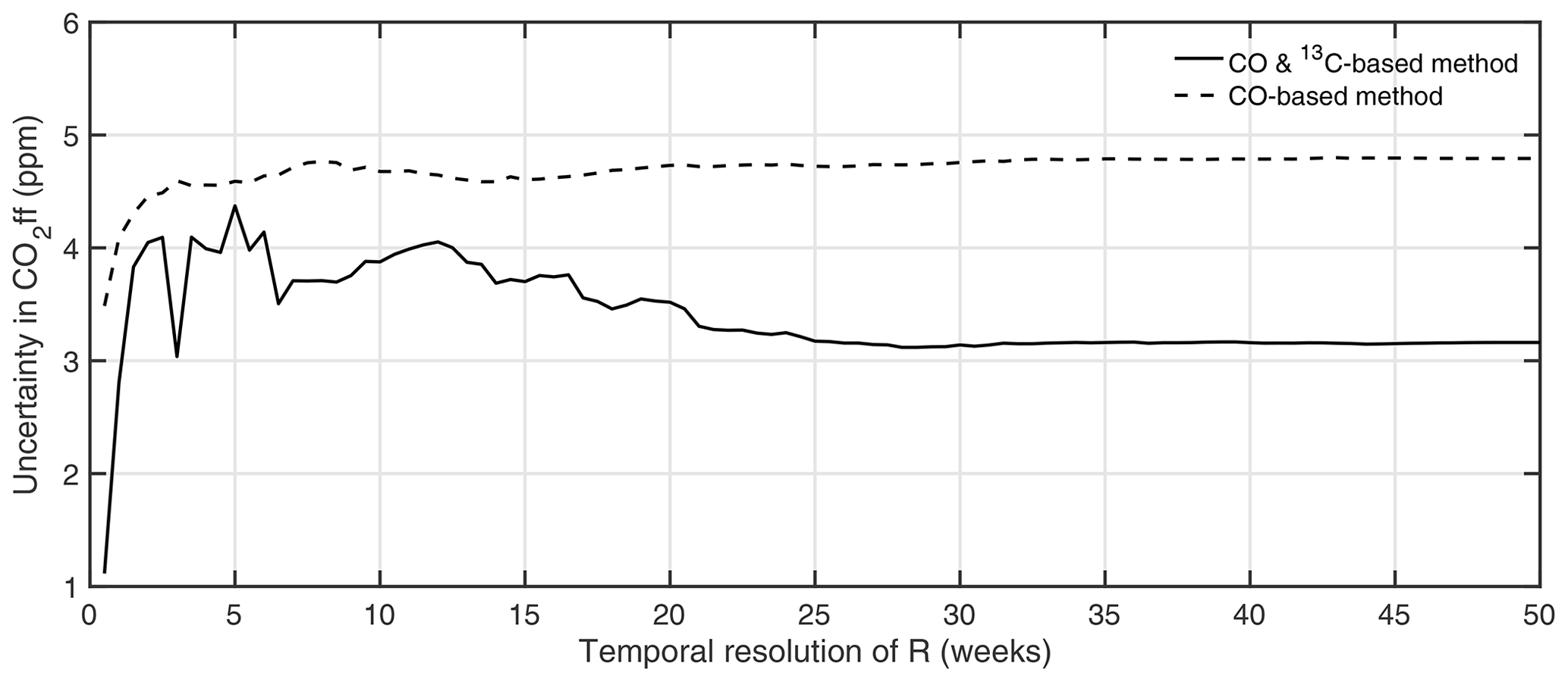
Figure 7Uncertainty in for varying temporal resolution of R (N weeks). R is determined for each data point solving Eq. (7) using CO, 13CO2 and 14CO2 observations within a moving window of 2N weeks. For the CO-based method, Rff is smoothed using a 2N-week moving window.
3.2 CO:CO2 emission ratio (R) values of biogenic, petroleum and natural gas sources
Monthly, site-based Rsrc varies between 5.5–11.4 ppb ppm−1 (Fig. 5), with a mean and standard deviation of 8.2 ± 1.6 ppb ppm−1 (relative SD = 19 %). Greater variability is seen in Rff (lower panel), with a mean and SD of 9.6 ± 2.1 ppm (relative SD = 22 %). To understand and predict the variation in Rff, we further divide the fossil fuel emissions into petroleum and natural gas emissions. Applying the calculated f values from Δ14CO2 and δ13CO2 observations (Sect. 2.2., Fig. 3), we solve Eq. (7) for each source's emission ratio, R (Table 2). Note that we exclude negative flask-based values of COxs (and corresponding Rsrc values) and CO2ff (and corresponding fff values) as non-physical. Likewise, positive δsrc values and values (and corresponding fpet and fng values) outside the range of 0–1 are also excluded. A bootstrapping method is used to calculate the mean and uncertainty of possible ratios. The ratios of petroleum (Rpet) and natural gas (Rng) combustion emissions are 12.2 ± 0.6 ppb ppm−1 and 2.3 ± 1.2 ppb ppm−1, respectively. As discussed above, the proportion of natural gas in fossil fuel emissions is bigger in summer, resulting in smaller Rff in summer at FUL and USC. We find the value of 1.8 ± 0.8 ppb ppm−1 for Rbio, which is non-zero because biofuel (mainly corn-based ethanol) in the gasoline in California with a large ratio signal is included in the biogenic sources, while respiratory ratios approach 0. A larger contribution of the biosphere with a low ratio in winter offsets the large Rff, lowering the variability in Rsrc at each site.
We compare our model-determined ratios of each source (Table 2) to bottom-up inventory-based estimates (Table 1). ratios of each source constrained from our model and the observational data approach agree well with the bottom-up inventory-based estimates. Sources contributing a high percentage of CO2 emissions strongly influence the total ratio. The ratio of petroleum combustion is greatly affected by on-road emissions and industrial emissions (contributing 60 % and 28 % of total petroleum CO2 emissions). Natural gas is mostly dominated by non-mobile emissions (electricity production, residential, commercial and industrial, sequentially), resulting in a low ratio.
3.3 Estimation of CO2ff based on CO and δ13CO2 observations
Table 2 shows the ratio and δ13C signature of each source. The combination of the R and δ signals reveals a distinct pattern for each source: the biosphere has low near-zero R, petroleum has high R and natural gas has low R. Petroleum and biosphere CO2 have similar δ values, whereas natural gas has a very low δ. By substituting these values into Eqs. (7)–(9), f′ values are calculated, and then we calculate by multiplying the sum of and by CO2xs measured every few days. We compare and to fff and Cff (determined using 14C observations) in Fig. 6. The assessment for each source is shown in Figs. S2 and S3. The R2 values are 0.63 and 0.90 for and , respectively.
If R values are allowed to vary in time, it is likely to improve the precision of the method. We calculate the uncertainty in for varying temporal resolutions of R (solid black line in Fig. 7). We find that the uncertainty increases when the size of the window increases from 1 week to 10 weeks; in other words, allowing temporal variation in R improves the precision of the method. However, the uncertainty decreases slightly beyond the 10-week window. This is likely caused by the reduction in the error of R values (not shown) as the number of observations used to find R (by solving Eq. 7) increases. In summary, the ideal flask sampling frequency for this method would be higher than every 2 weeks. In cases where this is impossible, it is better to assume constant R values.
The uncertainty in estimated using the CO-based method is also shown in Fig. 7 (dashed black line). The CO-based method also provides improved precision of the method when flask sampling is available at higher frequency. However, the CO- and δ13CO2-based method shows greater confidence than the CO-based method for the whole range of adjusted temporal resolution in R. When using constant R values (temporal resolution of 50 weeks), the uncertainty is 3.2 ppm (the 1σ standard deviation of differences between Cff and for the CO- and δ13CO2-based method, while it is 4.8 ppm for the CO-based method. This improvement is likely associated with the additional information provided by δ13CO2 that constrains the effective Rff and further separates fossil fuel sources into sub-categories (petroleum and natural gas sources).
We present a CO- and δ13CO2-based method to estimate CO2ff that is based on flask-based Δ14CO2 measurements. We applied the method to measurements from flask samples collected in the LA Basin every few days in the afternoon for more than 1 year (2015–2016). The proposed method was assessed by comparing it to a more traditional Δ14CO2-based method. The CO and δ13CO2 approach can be applied to continuous measurements of CO2, CO and δ13CO2, which can provide CO2ff estimates at higher temporal resolution and with greater accuracy than previously applied CO-based methods.
We analyzed three locations in the megacity of Los Angeles, partitioning observed CO2 enhancements (CO2xs) into biogenic, petroleum and natural gas sources. We observed a substantial biogenic signal that varies from −14 % to +25 % of CO2xs over the course of the year, with positive contributions in winter and negative contributions in summer due to net respiration and net photosynthesis, respectively. Furthermore, partitioning CO2ff into petroleum and natural gas combustion fractions revealed that natural gas combustion has the largest contribution in summer, potentially due to an increase in electricity generation at LA power plants for air-conditioning.
The data that support the findings of this study are available from John B. Miller (john.b.miller@noaa.gov) upon request.
The supplement related to this article is available online at: https://doi.org/10.5194/acp-23-14425-2023-supplement.
JK designed and executed the study. JBM, SJL and SEM provided the data. JK prepared the paper with contributions from all co-authors.
The contact author has declared that none of the authors has any competing interests.
Publisher's note: Copernicus Publications remains neutral with regard to jurisdictional claims made in the text, published maps, institutional affiliations, or any other geographical representation in this paper. While Copernicus Publications makes every effort to include appropriate place names, the final responsibility lies with the authors.
We acknowledge the support for this research provided by a USC Dornsife College Research Award to William M. Berelson.
Δ14C measurements and sample collection in Los Angeles were supported in part by a National Oceanic and Atmospheric Administration (NOAA) award (grant no. NA14OAR4310177), with additional contributions from NOAA Global Monitoring Laboratory funding and personnel. δ13C measurements were supported by NOAA including the Global Monitoring Laboratory and Climate Program Office. A portion of this work was performed at the Jet Propulsion Laboratory, California Institute of Technology, under contract with the National Aeronautics and Space Administration (grant no. 80NM0018D0004) and the National Institute of Standards and Technology.
This paper was edited by Eliza Harris and reviewed by Jocelyn Turnbull and one anonymous referee.
Ahn, D. Y., Hansford, J. R., Howe, S. T., Ren, X. R., Salawitch, R. J., Zeng, N., Cohen, M. D., Stunder, B., Salmon, O. E., Shepson, P. B., Gurney, K. R., Oda, T., Lopez-Coto, I., Whetstone, J., and Dickerson, R. R.: Fluxes of Atmospheric Greenhouse-Gases in Maryland (FLAGG-MD): Emissions of Carbon Dioxide in the Baltimore, MD-Washington, D.C. Area, J. Geophys. Res.-Atmos., 125, 1–23, https://doi.org/10.1029/2019JD032004, 2020.
Bakwin, P. S., Tans, P. P., Andres, J., and Conway, C. O.: Determination of the isotopic (13C/12C) discrimination of atmospheric, Global Biogeochem. Cy., 12, 555–562, 1998a.
Bakwin, P. S., Tans, P. P., White, J. W. C., and Andres, R. J.: Determination of the isotopic () discrimination of terrestrial biology from a global network of observations, Global Biogeochem. Cy., 12, 555–562, https://doi.org/10.1029/98GB02265, 1998b.
Bréon, F. M., Broquet, G., Puygrenier, V., Chevallier, F., Xueref-Remy, I., Ramonet, M., Dieudonné, E., Lopez, M., Schmidt, M., Perrussel, O., and Ciais, P.: An attempt at estimating Paris area CO2 emissions from atmospheric concentration measurements, Atmos. Chem. Phys., 15, 1707–1724, https://doi.org/10.5194/acp-15-1707-2015, 2015.
Cambaliza, M. O. L., Shepson, P. B., Caulton, D. R., Stirm, B., Samarov, D., Gurney, K. R., Turnbull, J., Davis, K. J., Possolo, A., Karion, A., Sweeney, C., Moser, B., Hendricks, A., Lauvaux, T., Mays, K., Whetstone, J., Huang, J., Razlivanov, I., Miles, N. L., and Richardson, S. J.: Assessment of uncertainties of an aircraft-based mass balance approach for quantifying urban greenhouse gas emissions, Atmos. Chem. Phys., 14, 9029–9050, https://doi.org/10.5194/acp-14-9029-2014, 2014.
Craig, H.: Isotopic standards for carbon and oxygen and correction factors for mass-spectrometric analysis of carbon dioxide, Geochim. Cosmochim. Acta, 12, 133–149, https://doi.org/10.1016/0016-7037(57)90024-8, 1957.
Djuricin, S., Pataki, D. E., and Xu, X.: A comparison of tracer methods for quantifying CO2 sources in an urban region, J. Geophys. Res., 115, 1–13, https://doi.org/10.1029/2009JD012236, 2010.
Fleisher, A. J., Long, D. A., Liu, Q., Gameson, L., and Hodges, J. T.: Optical Measurement of Radiocarbon below Unity Fraction Modern by Linear Absorption Spectroscopy, J. Phys. Chem. Lett., 8, 4550–4556, https://doi.org/10.1021/acs.jpclett.7b02105, 2017.
Gately, C. K. and Hutyra, L. R.: Large Uncertainties in Urban-Scale Carbon Emissions, J. Geophys. Res.-Atmos., 122, 11242-11260, https://doi.org/10.1002/2017JD027359, 2017.
Genoud, G., Lehmuskoski, J., Bell, S., Palonen, V., Oinonen, M., Koskinen-Soivi, M. L., and Reinikainen, M.: Laser Spectroscopy for Monitoring of Radiocarbon in Atmospheric Samples, Anal. Chem., 91, 12315–12320, https://doi.org/10.1021/acs.analchem.9b02496, 2019.
Gourdji, S. M., Karion, A., Lopez-Coto, I., Ghosh, S., Mueller, K. L., Zhou, Y., Williams, C. A., Baker, I. T., Haynes, K. D., and Whetstone, J. R.: A Modified Vegetation Photosynthesis and Respiration Model (VPRM) for the Eastern USA and Canada, Evaluated With Comparison to Atmospheric Observations and Other Biospheric Models, J. Geophys. Res.-Biogeosci., 127, e2021JG006290, https://doi.org/10.1029/2021JG006290, 2022.
Graven, H. D., Stephens, B. B., Guilderson, T. P., Campos, T. L., Schimel, D. S., Campbell, J. E., and Keeling, R. F.: Vertical profiles of biospheric and fossil fuel-derived CO2 and fossil fuel CO2: CO ratios from airborne measurements of Δ14C, CO2 and CO above Colorado, USA, Tellus B, 61, 536–546, https://doi.org/10.1111/j.1600-0889.2009.00421.x, 2009.
Gurney, K. R., Patarasuk, R., Liang, J., Song, Y., O'Keeffe, D., Rao, P., Whetstone, J. R., Duren, R. M., Eldering, A., and Miller, C.: The Hestia fossil fuel CO2 emissions data product for the Los Angeles megacity (Hestia-LA), Earth Syst. Sci. Data, 11, 1309–1335, https://doi.org/10.5194/essd-11-1309-2019, 2019.
Hardiman, B. S., Wang, J. A., Hutyra, L. R., Gately, C. K., Getson, J. M., and Friedl, M. A.: Accounting for urban biogenic fluxes in regional carbon budgets, Sci. Total Environ., 592, 366–372, https://doi.org/10.1016/j.scitotenv.2017.03.028, 2017.
He, L., Zeng, Z., Pongetti, T. J., Wong, C., Liang, J., Gurney, K. R., Newman, S., Yadav, V., Verhulst, K. R., Miller, C. E., Duren, R., Frankenberg, C., Wennberg, P. O., Shia, R., Yung, Y. L., and Sander, S. P.: Atmospheric Methane Emissions Correlate With Natural Gas Consumption From Residential and Commercial Sectors in Los Angeles, Geophys. Res. Lett., 46, 8563–8571, https://doi.org/10.1029/2019gl083400, 2019.
Heimburger, A., Harvey, R., Shepson, P. B., Stirm, B. H., Gore, C., Turnbull, J. C., Cambaliza, M. O. L., Salmon, O. E., Kerlo, A.-E. M., Lavoie, T. N., Davis, K. J., Lauvaux, T., Karion, A., Sweeney, C., Brewer, W. A., Hardesty, R. M., and Gurney, K. R.: Assessing the optimized precision of the aircraft mass balance method for measurement of urban greenhouse gas emission rates through averaging, Elem. Sci. Anth., 5, 26, https://doi.org/10.1525/elementa.134, 2017.
IPCC: Contribution of Working Group III to the Fifth Assessment Report of the Intergovernmental Panel on Climate Change, Climate Change 2014: Mitigation of Climate Change, Cambridge University Press, https://doi.org/10.1017/CBO9781107415416, 2014.
Lauvaux, T., Miles, N. L., Deng, A., Richardson, S. J., Cambaliza, M. O., Davis, K. J., Gaudet, B., Gurney, K. R., Huang, J., O'Keefe, D., Song, Y., Karion, A., Oda, T., Patarasuk, R., Razlivanov, I., Sarmiento, D., Shepson, P., Sweeney, C., Turnbull, J. C., and Wu, K.: High-resolution atmospheric inversion of urban CO2 emissions during the dormant season of the Indianapolis flux experiment (INFLUX), J. Geophys. Res., 121, 5213–5236, https://doi.org/10.1002/2015JD024473, 2016.
Lauvaux, T., Gurney, K. R., Miles, N. L., Davis, K. J., Richardson, S. J., Deng, A., Nathan, B. J., Oda, T., Wang, J. A., Hutyra, L., and Turnbull, J. C.: Policy-relevant assessment of urban CO2emissions, Environ. Sci. Technol., 54, 10237–10245, https://doi.org/10.1021/acs.est.0c00343, 2020.
Lehman, S. J., Miller, J. B., Wolak, C., Southon, J., Tans, P. P., Montzka, S. A., Sweeney, C., Andrews, A., LaFranchi, B., Guilderson, T. P., and Turnbull, J. C.: Allocation of Terrestrial Carbon Sources Using 14 CO2: Methods, Measurement, and Modeling, Radiocarbon, 55, 1484–1495, https://doi.org/10.1017/s0033822200048414, 2013.
Levin, I. and Karstens, U.: Inferring high-resolution fossil fuel CO2 records at continental sites from combined 14CO2 and CO observations, Tellus, Ser. B Chem. Phys. Meteorol., 59, 245–250, https://doi.org/10.1111/j.1600-0889.2006.00244.x, 2007.
Levin, I., Kromer, B., Schmidt, M., and Sartorius, H.: A novel approach for independent budgeting of fossil fuel CO2 over Europe by 14CO2 observations, Geophys. Res. Lett., 30, 1–5, https://doi.org/10.1029/2003GL018477, 2003.
Lopez, M., Schmidt, M., Delmotte, M., Colomb, A., Gros, V., Janssen, C., Lehman, S. J., Mondelain, D., Perrussel, O., Ramonet, M., Xueref-Remy, I., and Bousquet, P.: CO, NOx and 13CO2 as tracers for fossil fuel CO2: results from a pilot study in Paris during winter 2010, Atmos. Chem. Phys., 13, 7343–7358, https://doi.org/10.5194/acp-13-7343-2013, 2013.
Mays, K. L., Shepson, P. B., Stirm, B. H., Karion, A., Sweeney, C., and Gurney, K. R.: Aircraft-based measurements of the carbon footprint of Indianapolis, Environ. Sci. Technol., 43, 7816–7823, https://doi.org/10.1021/es901326b, 2009.
McCartt, A. D. and Jiang, J.: Room-Temperature Optical Detection of 14CO2 below the Natural Abundance with Two-Color Cavity Ring-Down Spectroscopy, ACS Sensors, 7, 3258–3264, https://doi.org/10.1021/acssensors.2c01253, 2022.
Mcdonald, B. C., McBride, Z. C., Martin, E. W., and Harley, R. A.: High-resolution mapping of motor vehicle carbon dioxide emissions, J. Geophys. Res.-Atmos., 119, 5283–5298, https://doi.org/10.1002/2013JD021219, 2014.
Miller, J. B., Lehman, S. J., Montzka, S. A., Sweeney, C., Miller, B. R., Karion, A., Wolak, C., Dlugokencky, E. J., Southon, J., Turnbull, J. C., and Tans, P. P.: Linking emissions of fossil fuel CO2 and other anthropogenic trace gases using atmospheric 14CO2, J. Geophys. Res.-Atmos., 117, D08302, https://doi.org/10.1029/2011JD017048, 2012.
Miller, J. B., Lehman, S. J., Verhulst, K. R., Miller, C. E., Duren, R. M., Yadav, V., Newman, S., and Sloop, C. D.: Large and seasonally varying biospheric CO2 fluxes in the Los Angeles megacity revealed by atmospheric radiocarbon, P. Natl. Acad. Sci. USA, 117, 26681–26687, https://doi.org/10.1073/pnas.2005253117, 2020.
Newman, S., Xu, X., Affek, H. P., Stolper, E., and Epstein, S.: Changes in mixing ratio and isotopic composition of CO2 in urban air from the Los Angeles basin, California, between 1972 and 2003, J. Geophys. Res.-Atmos., 113, 1–15, https://doi.org/10.1029/2008JD009999, 2008.
Newman, S., Jeong, S., Fischer, M. L., Xu, X., Haman, C. L., Lefer, B., Alvarez, S., Rappenglueck, B., Kort, E. A., Andrews, A. E., Peischl, J., Gurney, K. R., Miller, C. E., and Yung, Y. L.: Diurnal tracking of anthropogenic CO2 emissions in the Los Angeles basin megacity during spring 2010, Atmos. Chem. Phys., 13, 4359–4372, https://doi.org/10.5194/acp-13-4359-2013, 2013.
Newman, S., Xu, X., Gurney, K. R., Hsu, Y. K., Li, K. F., Jiang, X., Keeling, R., Feng, S., O'Keefe, D., Patarasuk, R., Wong, K. W., Rao, P., Fischer, M. L., and Yung, Y. L.: Toward consistency between trends in bottom-up CO2 emissions and top-down atmospheric measurements in the Los Angeles megacity, Atmos. Chem. Phys., 16, 3843–3863, https://doi.org/10.5194/acp-16-3843-2016, 2016.
Sargent, M., Barrera, Y., Nehrkorn, T., Hutyra, L. R., Gately, C. K., Jones, T., McKain, K., Sweeney, C., Hegarty, J., Hardiman, B., and Wofsy, S. C.: Anthropogenic and biogenic CO2 fluxes in the Boston urban region, P. Natl. Acad. Sci. USA, 115, 7491–7496, https://doi.org/10.1073/pnas.1803715115, 2018.
Staufer, J., Broquet, G., Bréon, F.-M., Puygrenier, V., Chevallier, F., Xueref-Rémy, I., Dieudonné, E., Lopez, M., Schmidt, M., Ramonet, M., Perrussel, O., Lac, C., Wu, L., and Ciais, P.: The first 1-year-long estimate of the Paris region fossil fuel CO2 emissions based on atmospheric inversion, Atmos. Chem. Phys., 16, 14703–14726, https://doi.org/10.5194/acp-16-14703-2016, 2016.
Stuiver, M. and Polach, H. A.: Discussion: Reporting of 14C Data, Radiocarbon, 19, 355–363, 1977.
Super, I., Dellaert, S. N. C., Visschedijk, A. J. H., and Denier van der Gon, H. A. C.: Uncertainty analysis of a European high-resolution emission inventory of CO2 and CO to support inverse modelling and network design, Atmos. Chem. Phys., 20, 1795–1816, https://doi.org/10.5194/acp-20-1795-2020, 2020.
Sweeney, C., Karion, A., Wolter, S., Newberger, T., Guenther, D., Higgs, J. A., Andrews, A. E., Lang, P. M., Neff, D., Dlugokencky, E., Miller, J. B., Montzka, S. A., Miller, B. R., Masarie, K. A., Biraud, S. C., Novelli, P. C., Crotwell, M., Crotwell, A. M., Thoning, K., and Tans, P. P.: Seasonal climatology of CO2 across North America from aircraft measurements in the NOAA/ESRL Global Greenhouse Gas Reference Network, J. Geophys. Res.-Atmos., 120, 5155–5190, https://doi.org/10.1002/2014JD022591, 2015.
Turnbull, J. C., Miller, J. B., Lehman, S. J., Tans, P. P., Sparks, R. J., and Southon, J.: Comparison of 14CO2, CO, and SF6 as tracers for recently added fossil fuel CO2 in the atmosphere and implications for biological CO2 exchange, Geophys. Res. Lett., 33, 2–6, https://doi.org/10.1029/2005GL024213, 2006.
Turnbull, J. C., Karion, A., Fischer, M. L., Faloona, I., Guilderson, T., Lehman, S. J., Miller, B. R., Miller, J. B., Montzka, S., Sherwood, T., Saripalli, S., Sweeney, C., and Tans, P. P.: Assessment of fossil fuel carbon dioxide and other anthropogenic trace gas emissions from airborne measurements over Sacramento, California in spring 2009, Atmos. Chem. Phys., 11, 705–721, https://doi.org/10.5194/acp-11-705-2011, 2011.
Turnbull, J. C., Sweeney, C., Karion, A., Newberger, T., Lehman, S. J., Tans, P. P., Davis, K. J., Lauvaux, T., Miles, N. L., Richardson, S. J., Cambaliza, M. O., Shepson, P. B., Gurney, K. R., Patarasuk, R., and Razlivanov, I.: Toward quantification and source sector identification of fossil fuel CO2 emissions from an urban area: Results from the INFLUX experiment, J. Geophys. Res., 120, 292–312, https://doi.org/10.1002/2014JD022555, 2015.
Turnbull, J. C., DeCola, P., Mueller, K., and Vogel, F.: IG3IS Urban Greenhouse Gas Emission Observation and Monitoring Best Research Practices, World Meteorological Organization, https://ig3is.wmo.int/ (last access: 25 October 2023), 1 August 2022.
Turner, A. J., Kim, J., Fitzmaurice, H., Newman, C., Worthington, K., Chan, K., Wooldridge, P., Köhler, P., Frankenberg, C., and Cohen, R. C.: Observed impacts of COVID-19 on urban CO2 emissions, Geophys. Res. Lett., 47, e2020GL090037, https://doi.org/10.1029/2020GL090037, 2020.
Vardag, S. N., Gerbig, C., Janssens-Maenhout, G., and Levin, I.: Estimation of continuous anthropogenic CO2: model-based evaluation of CO2, CO, δ13C(CO2) and Δ14C(CO2) tracer methods, Atmos. Chem. Phys., 15, 12705–12729, https://doi.org/10.5194/acp-15-12705-2015, 2015.
Vaughn, B. H., Miller, J. B., Ferretti, D. F., and White, J. W. C.: Stable isotope measurements of atmospheric CO2 and CH4, in: Handbook of Stable Isotope Analytical Techniques, https://doi.org/10.1016/B978-044451114-0/50016-8, 2004.
Vimont, I. J., Turnbull, J. C., Petrenko, V. V., Place, P. F., Sweeney, C., Miles, N., Richardson, S., Vaughn, B. H., and White, J. W. C.: An improved estimate for the δ13C and δ18O signatures of carbon monoxide produced from atmospheric oxidation of volatile organic compounds, Atmos. Chem. Phys., 19, 8547–8562, https://doi.org/10.5194/acp-19-8547-2019, 2019.
Vogel, F. R., Hammer, S., Steinhof, A., Kromer, B., and Levin, I.: Implication of weekly and diurnal 14C calibration on hourly estimates of CO-based fossil fuel CO2 at a moderately polluted site in southwestern Germany, Tellus B, 62, 512–520, https://doi.org/10.1111/j.1600-0889.2010.00477.x, 2010.
Vogel, F. R., Frey, M., Staufer, J., Hase, F., Broquet, G., Xueref-Remy, I., Chevallier, F., Ciais, P., Sha, M. K., Chelin, P., Jeseck, P., Janssen, C., Té, Y., Groß, J., Blumenstock, T., Tu, Q., and Orphal, J.: XCO2 in an emission hot-spot region: the COCCON Paris campaign 2015, Atmos. Chem. Phys., 19, 3271–3285, https://doi.org/10.5194/acp-19-3271-2019, 2019.
Winbourne, J. B., Smith, I. A., Stoynova, H., Kohler, C., Gately, C. K., Logan, B. A., Reblin, J., Reinmann, A., Allen, D. W., and Hutyra, L. R.: Quantification of Urban Forest and Grassland Carbon Fluxes Using Field Measurements and a Satellite-Based Model in Washington DC/Baltimore Area, J. Geophys. Res.-Biogeosci., 127, e2021JG006568, https://doi.org/10.1029/2021JG006568, 2022.
Wu, D., Lin, J. C., Duarte, H. F., Yadav, V., Parazoo, N. C., Oda, T., and Kort, E. A.: A model for urban biogenic CO2 fluxes: Solar-Induced Fluorescence for Modeling Urban biogenic Fluxes (SMUrF v1), Geosci. Model Dev., 14, 3633–3661, https://doi.org/10.5194/gmd-14-3633-2021, 2021.