the Creative Commons Attribution 4.0 License.
the Creative Commons Attribution 4.0 License.
 | 25 Jan 2023
Microphysical, macrophysical, and radiative responses of subtropical marine clouds to aerosol injections
Je-Yun Chun
Peter Blossey
Sarah J. Doherty
Ship tracks in subtropical marine low clouds are simulated and investigated using large-eddy simulations. Five variants of a shallow subtropical stratocumulus-topped marine boundary layer (MBL) are chosen to span a range of background aerosol concentrations and variations in free-tropospheric moisture. Idealized time-invariant meteorological forcings and approximately steady-state aerosol concentrations constitute the background conditions. We investigate processes controlling cloud microphysical, macrophysical, and radiative responses to aerosol injections. For the analysis, we use novel methods to decompose the liquid water path (LWP) adjustment into changes in cloud and boundary-layer properties and to decompose the cloud radiative effect (CRE) into contributions from cloud macro- and microphysics. The key results are that (a) the cloud-top entrainment rate increases in all cases, with stronger increases for thicker than thinner clouds; (b) the drying and warming induced by increased entrainment is offset to differing degrees by corresponding responses in surface fluxes, precipitation, and radiation; (c) MBL turbulence responds to changes caused by the aerosol perturbation, and this significantly affects cloud macrophysics; (d) across 2 d of simulation, clouds were brightened in all cases. In a pristine MBL, significant drizzle suppression by aerosol injections results not only in greater water retention but also in turbulence intensification, leading to a significant increase in cloud amount. In this case, Twomey brightening is strongly augmented by an increase in cloud thickness and cover. In addition, a reduction in the loss of aerosol through coalescence scavenging more than offsets the entrainment dilution. This interplay precludes estimation of the lifetime of the aerosol perturbation. The combined responses of cloud macro- and microphysics lead to 10–100 times more effective cloud brightening in these cases relative to those in the non-precipitating MBL cases. In moderate and polluted MBLs, entrainment enhancement makes the boundary layer drier, warmer, and more stratified, leading to a decrease in cloud thickness. This LWP response offsets the greatest fraction of the Twomey brightening in a moderately moist free troposphere. This finding differs from previous studies that found larger offsets in a drier free troposphere, and it results from a greater entrainment enhancement of initially thicker clouds, so the offsetting effects are weaker. The injected aerosol lifetime in cases with polluted MBLs is estimated to be 2–3 d, which is much longer than estimates of typical ship track lifetimes from satellite images.
- Article
(7943 KB) - Full-text XML
-
Supplement
(1508 KB) - BibTeX
- EndNote


Stratocumulus clouds cover extensive areas of the ocean surface and influence the climate system primarily by enhancing the reflection of incoming solar radiation back to space (e.g., Hartmann and Short, 1980). That is, clouds are brighter than open ocean when seen from space. Cloud brightness (i.e., solar reflectivity) is determined by cloud macrophysical (coverage and thickness) and microphysical (droplet size) properties. Anthropogenic pollution increases cloud condensation nuclei (CCN) concentrations, which leads to more numerous and smaller cloud droplets (Twomey, 1974). For a fixed liquid water path (LWP), cloud optical thickness increases sublinearly with the cloud droplet number concentration (Nc), a behavior known as the Twomey effect (Twomey, 1977). Observational and modeling studies provide convincing evidence that anthropogenic aerosol forcing by aerosol–cloud interactions masks a significant fraction of the forcing from increases in well-mixed greenhouse gases (e.g., Zelinka et al., 2014; Bellouin et al., 2020; Forster et al., 2021).
Although the Twomey effect results in cloud brightening, cloud macrophysical responses to aerosols (known as cloud adjustments) remain highly uncertain and have the potential to enhance or offset Twomey brightening. The cloud fraction may increase or decrease with aerosol depending on meteorological conditions and the size and concentration of both background and injected aerosol. In a precipitating boundary layer, aerosol increases reduce cloud droplet size and collision–coalescence efficiency, leading to precipitation suppression (Wood, 2012). Taken alone, precipitation suppression should allow the retention of liquid water in clouds, potentially increasing the LWP and cloud cover (Albrecht, 1989). In a non-precipitating boundary layer, on the other hand, water retention is weak. Increased droplet surface area reduces both the timescale for the evaporation of liquid water (Wang et al., 2003) and the rate of sedimentation of condensate away from cloud top (Bretherton et al., 2007; Ackerman et al., 2009). Both effects are expected to enhance the cloud-top entrainment rate (Ackerman et al., 2004). In most circumstances, entrainment warming and drying results in thinner clouds with a lower LWP (Wood, 2007). Thus, cloud adjustments can either be positive or negative depending upon the nature of the cloud into which aerosol is introduced, the moisture of the free-tropospheric air overlying the cloud, and the background and added aerosol properties (Ackerman et al., 2004; Wood, 2007; Glassmeier et al., 2021; Hoffmann and Feingold, 2021).
Recent observational and modeling studies of so-called “natural experiments”, such as of shipping and pollution plumes, yield a wide range of estimates of the contribution of cloud adjustments to overall aerosol forcing. Observations over polluted and adjacent unperturbed regions have shown that the average LWP adjustment is negative, ranging from 3 % to 20 % (Toll et al., 2019; Diamond et al., 2020; Trofimov et al., 2020), and it may offset up to 30 % of the Twomey effect. Other studies have investigated the Nc–LWP relationship more generally using satellite observations (Gryspeerdt et al., 2019) and large-eddy simulation (LES) modeling (Glassmeier et al., 2021), estimating that negative LWP adjustments may offset as much as 60 % of the Twomey brightening. Glassmeier et al. (2021), however, argued that estimates using ship track data overestimate albedo increases associated with an anthropogenically enhanced Nc by up to 200 %, because the lifetime of the ship track (typically ∼8 h) is usually shorter than the timescale by which clouds relax to an equilibrium state (∼20 h; see Eastman et al., 2016).
Better constraining the cloud responses to aerosols is of interest because the radiative forcing from only a small change in the coverage and thickness of stratocumulus clouds is comparable to the warming resulting from doubling atmospheric carbon dioxide (Randall et al., 1984). This fact, and clouds' known strong sensitivity to aerosol, led to the idea that deliberately injecting CCN into subtropical low marine clouds might enhance cloud albedo and offset global warming (Latham, 1990). This climate intervention approach is commonly referred to as marine cloud brightening (MCB). Modeling studies with global climate models (GCMs) to test the potential efficacy of MCB have been conducted by enhancing the Nc or reducing the effective radius of cloud drops (re). They have shown that cooling sufficient to offset a significant fraction of global warming caused by doubling of preindustrial CO2 is potentially achievable (e.g., Latham et al., 2008, 2012; Rasch et al., 2009; Ahlm et al., 2017; Stjern et al., 2018). Salter et al. (2008) estimated that an injection rate of 1.45×10⁶ particles over all marine regions covered by exposed low clouds would produce a sufficient Twomey cloud radiative effect perturbation of −3.7 W m−2, which is comparable to the positive radiative forcing from a doubling of preindustrial CO2. GCMs, however, are not able to fully represent the complexity of aerosol–cloud interactions. For instance, most GCMs show that global-scale aerosol perturbation induces positive LWP adjustment on average (Lohmann and Feichter, 2005), which runs counter to observational evidence.
LES models can resolve most processes relevant to aerosol–cloud–precipitation interactions, allowing more accurate simulations of cloud responses to the addition of aerosols, and for attribution of the drivers behind these adjustments under a range of local meteorological conditions (e.g., Wang and Feingold, 2009; Wang et al., 2011; Berner et al., 2015; Possner et al., 2018). Using LES models, Wang and Feingold (2009) and Wang et al. (2011) showed that sharp gradients in precipitation generated by spatially variable aerosol concentrations induce a mesoscale circulation, which affects cloud properties. Wang et al. (2011) showed that the albedo perturbation produced by aerosol injection strongly depends on the background cloud droplet concentration and meteorological conditions. Using an LES, Berner et al. (2015) successfully simulated an observed ship track in the collapsed marine boundary layer sampled by aircraft. Sensitivity tests with LES models to changes in background aerosol number concentration are consistent with observations: positive LWP adjustments tend to occur under pristine conditions, and negative adjustments occur in polluted boundary layers (e.g., Lohmann and Feichter, 2005; Wang et al., 2011; Berner et al., 2015). Possner et al. (2018) investigated ship tracks in deep open-cell stratocumuli, showing that, although ship tracks are rarely visible in satellite retrievals in deep boundary layers (e.g., Durkee et al., 2000; Coakley et al., 2000), their radiative effect could be significant. While these studies have provided useful new insights, there are still many processes regarding how clouds respond to the addition of CCN in a plume that need to be better quantified; these include details on entrainment enhancement, the role of other processes controlling cloud properties (e.g., turbulence, surface flux, precipitation, and radiation), and the full temporal evolution of cloud responses.
This study investigates the processes controlling cloud microphysical, macrophysical, and radiative responses to aerosol injection in marine boundary layers (MBLs) under different background aerosol concentrations and a range of lower free-tropospheric moisture using LES modeling. Two novel methods are used to quantitatively decompose the cloud adjustments into the contributions from different processes and to decompose the cloud radiative effect (CRE) into the contributions from changes in the cloud droplet number concentration (Nc), LWP, and cloud fraction (CF).
2.1 Model formulation
This study uses version 6.10 of the System for Atmospheric Modeling (SAM), a non-hydrostatic anelastic model (Khairoutdinov and Randall, 2003). Three-dimensional simulations are used with a horizontal grid resolution of 50 m and a vertical grid resolution that gradually varies from 5 m at 400–800 m altitude (where clouds form) to 15 m near the surface and to 70 m at the top (1.55 km) of the vertical domain. The model time step is adaptive with a typical value of ∼0.5 s. Periodic boundary conditions in both the x and y dimensions are used. The upper part of the domain includes a sponge layer to damp gravity waves and prevent artificial reflection from the upper boundary. The sub-grid-scale turbulence is represented using a 1.5-order turbulent closure model with a prognostic formulation of turbulent kinetic energy. Advection of all scalars is calculated using an advection scheme that preserves monotonicity (Blossey and Durran, 2008). The total water mixing ratio (qt) and liquid static energy () are conserved under phase changes. Here, cp is the specific heat of air at constant pressure, T is the temperature, z is the altitude, g is the gravitational acceleration, L is the latent heat of evaporation of water, and ql is the liquid water content. Hereafter, will be used as a conserved variable. Radiation, entrainment mixing, surface fluxes, and precipitation influence the prognostic variables. Radiative transfer (shortwave and thermal infrared) is calculated using the Rapid Radiative Transfer Model for GCM applications (RRTMG; Mlawer et al., 1997), which utilizes a droplet effective radius (re) diagnosed from microphysical variables related to cloud. Sensible and latent heat fluxes from the ocean surface are calculated in each grid box based on Monin–Obukhov theory.
The two-moment Morrison microphysics scheme (Morrison and Grabowski, 2008) with autoconversion and accretion parameterized following Khairoutdinov and Kogan (2000) predicts the number concentrations and mixing ratios of cloud and rain droplets. When the water vapor mixing ratio (qv) is greater than the saturation mixing ratio, condensation is calculated using saturation adjustment. Evaporation of drizzle is explicitly represented, but vapor deposition onto drizzle is not. Ice-phase hydrometeor species are not required because the simulation domain is below the freezing level everywhere.
A bulk aerosol scheme (Berner et al., 2013) that predicts the number and dry mass of a single lognormal accumulation mode is combined with the modeled cloud microphysics to simulate the aerosol life cycle and, therefore, more faithfully represent aerosol–cloud–precipitation interactions. The scheme represents activation (Abdul-Razzak and Ghan, 2000), autoconversion, accretion, precipitation evaporation, scavenging of interstitial aerosol by cloud and rain (see appendix in Berner et al., 2013), droplet sedimentation, and surface fluxes. The number and mass fluxes of sea-salt spray is diagnosed based on the wind speed (Clarke et al., 2006) with a single, lognormal accumulation mode with a mean dry diameter of 255 nm. Note that the size of the aerosol produced by surface flux has been corrected from that in Berner et al. (2013). Cloud droplets are activated from this single lognormal aerosol size distribution, defined by the number and mass of aerosol and the geometric standard deviation of 1.5. Above-inversion aerosol has a prescribed size of 200 nm. There is no representation of the Aitken mode.
2.2 Simulation descriptions
Model simulations in this study are based on an idealized stratocumulus case study used in the Cloud Feedbacks Model Intercomparison Project/Global Atmospheric Systems Studies Intercomparison of Large-Eddy and Single-Column Models (CGILS). Among the cases CGILS considered, we focus on S12 (Blossey et al., 2013), which is derived from monthly mean (July 2003) data from the ECMWF ERA-Interim reanalysis (ERA) near the Californian coast (35∘ N, 125∘ W). Unlike in Blossey et al. (2013), solar insolation varies diurnally in these simulations, with corresponding changes in solar zenith angle. Although these simulations use constant-in-time Eulerian forcings (Zhang et al., 2012), they are intended to represent the evolution of an air mass after aerosol injection for 39.5 h downstream following the aerosol injection. While such an air mass would be expected to experience changing forcings over that time period, we choose steady forcings in order to be able to both characterize the effect of aerosol injection and more clearly attribute it to key processes in the presence of a diurnal cycle on an important MBL cloud regime. In future work, we plan to evaluate the effect of aerosol injection on Lagrangian case studies of stratocumulus-to-cumulus transitions (e.g., Sandu and Stevens, 2011; Blossey et al., 2021).
This study investigates the effects of aerosol injections into five variants of the CGILS S12 case. The variants are designed to explore how cloud responses depend upon different aerosol background conditions and lower free-troposphere water vapor concentrations. The background aerosol is initially uniformly distributed in the model. After model spin-up, spatial variations in background aerosol concentrations develop (e.g., as a result of interactions with clouds). The cases are designed to have aerosol concentrations in the control case (no aerosol injection) that are, on average across the domain, in approximately steady state over the 2 d period. This avoids interpretation issues that would be inevitable if the background aerosol concentrations were strongly evolving with time and also facilitates the attribution of cloud responses to specific processes. An attempt was also made to ensure that boundary-layer depth and cloud properties do not strongly drift over time. To avoid strong drifts, lower free-troposphere aerosol Na,FT and large-scale divergence D values were adjusted to produce quasi-steady-state conditions in the MBL.
Table 1Conditions used for the Pristine6, Middle6, Polluted6, Polluted3.5, and Polluted1.5 cases. The upper section of the table summarizes the initial and boundary conditions, the middle section summarizes the quasi-steady-state conditions in Ctrl runs, and the lower section summarizes the information on aerosol injections.

Initial and boundary conditions for the five variant cases are shown in Table 1. All other meteorological drivers are the same across all of the cases. The Pristine6, Middle6, and Polluted6 cases produce different precipitation regimes: precipitating, weakly precipitating, and non-precipitating stratocumulus, respectively. Polluted6, Polluted3.5, and Polluted1.5 have the same aerosol initial and boundary conditions but have free tropospheric water vapor mixing ratios qFT of 6.0, 3.5, and 1.5 g kg−1, respectively. All three of the polluted cases produce negligible precipitation. Simulations are performed for a 96 km × 9.6 km domain for the Pristine6 and Middle6 cases and for a 48 km × 9.6 km domain for the Polluted6, Polluted3.5, and Polluted1.5 cases. The wider domains for the Pristine6 and Middle6 are used to ensure that a significant portion of the domain remains free of injected aerosol for the entire run in order to allow an analysis of mesoscale interactions between the track and surrounding clouds, which are more significant in the precipitating cases. All of the cases are run for 39.5 h after spin-up, which covers the first daytime and nighttime periods as well as the second daytime period, which will be referred as to Day 1, Night, and Day 2, respectively.
The model is spun up for 12 h, from 16:00 to 04:00 LT. Two branched runs with (Plume) and without (Ctrl) aerosol injection are then produced for each case. In the Plume runs, a point sprayer travels once across the center of the x axis (long dimension) along the y axis (short dimension) with a domain-relative speed of 10.5 m s−1 for 914 s. This is consistent with the model domain representing a 9.6 km wide slab of an air mass moving at 10.5 m s−1 over a stationary point-source injection site. This wind speed is similar to the near-surface wind speed in Blossey et al. (2013) (8.3 m s−1), and it allows for a moderate increase in winds with altitude in the MBL. The mean modal dry diameter of the injected aerosol is 205 nm. The injection rate is 1016 s−1 in Pristine6, in Middle6, and in the polluted cases in order to produce a roughly consistent fractional increase in the mean aerosol concentration, 〈Na〉, across the cases. The injection rates used in this study are comparable to those suggested in previous studies (e.g., Salter et al., 2008; Wang et al., 2011; Wood, 2021). The initial 〈Na〉 perturbation () is given in Table 1.
The quasi-steady-state conditions are also summarized in Table 1. The buoyancy jump across the inversion (Δbt) is strongest in the polluted cases where the large-scale subsidence is strongest. The jump in the total water mixing ratio (Δqt) largely varies with qFT, from −Δqt of 3.6–3.8 g kg−1 in the moist case to 7.3 g kg−1 in the driest case, Polluted1.5. In-cloud droplet concentration (NCCLD) is similar to 〈Na〉 in the Ctrl cases (Table 1).
3.1 General description
In the following two subsections, general characteristics of the cloud fields in the baseline (Ctrl) runs and the perturbations to the clouds in the aerosol injection (Plume) runs are described.
Table 2Spatiotemporal averages from the baseline (Ctrl) simulations of the in-cloud LWPCLD, cloud fraction (CF), surface precipitation rate (Rsfc), cloud-base precipitation rate (Rcb), effective radius of cloud drops (re), entrainment rate (we), and inversion height (zinv) for the simulated cases. The first, second, and third values represent averages across Day 1, Night, and Day 2, respectively, with the standard deviations shown in square brackets.

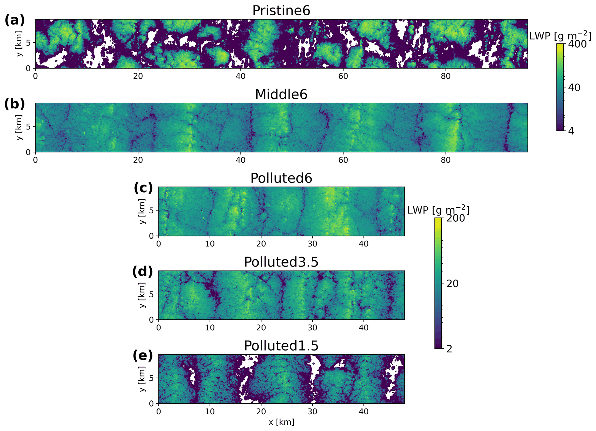
Figure 1Horizontal fields of the LWP at local noon (12:08 LT) on Day 1 in the Ctrl run for the Pristine6, Middle6, Polluted6, Polluted3.5, and Polluted1.5 cases.

3.1.1 Baseline (Ctrl) runs
Table 2 shows the averages and standard deviations of meteorological conditions during Day 1, Night, and Day 2 in the Ctrl runs for each case. As observed in subtropical marine stratocumulus (Wood et al., 2002), the LES runs show a strong diurnal cycle in cloud properties. Figures 1 and 2 show the cloud LWP across the model domain in each case during Day 1 and Night, respectively, for the Ctrl runs. In all cases, mesoscale roll convection develops, similar to that seen in the LES runs of a case study using aircraft-observed fields (Berner et al., 2015). In the Pristine6 runs, the roll structure is less coherent, especially during daytime, and the cloud structure more closely resembles open cellular convection. This change in the cloud field organization is likely caused by cloud-base precipitation. Solar absorption may also help to break the roll structure (Chlond, 1992; Müller and Chlond, 1996; Glendening, 1996; Berner et al., 2015).
During daytime, the in-cloud LWP (LWPCLD) is lower than at night (Table 2), as solar absorption weakens the net radiative cooling at cloud top, which is the primary source of turbulence in marine low clouds. It is notable that the LWPCLD in the Polluted3.5 and Polluted1.5 runs is much lower than 60 g m−2, contradicting the argument by Hoffmann et al. (2020) that a LWP is difficult to sustain in steady state. Our inclusion of the diurnal cycle (in contrast to Hoffmann et al., 2020) may permit lower LWP values to be sustained in our cases, but this is unclear. The CF in Pristine6 also varies diurnally from ∼50 % during the day to ∼80 % at night. During the daytime, weak turbulence is unable to supply water vapor from the subcloud to the cloud layer so that the cloud is depleted by drizzle. During the night, the turbulence is intensified and cloud water is recovered. The Middle6 and Polluted6 cases remain overcast through the entire day, without stabilization of the boundary layer due to drizzle evaporation. As the free troposphere (FT) becomes drier, the CF decreases because the lifting condensation level (LCL) becomes closer to the inversion due to the incorporation of dry free-tropospheric air into the boundary layer.
For the Pristine6 run, the cloud-base precipitation rate Rcb varies diurnally from 0.40 mm d−1 during the day to 0.81 mm d−1 at night. Rcb in the Middle6 run is much weaker due to the low coalescence efficiency of the smaller cloud droplets, and this precipitation is too weak to reach the surface. Rcb in the three polluted cases is negligible (). Similarly, the surface precipitation rate Rsfc in the Pristine6 run changes from 0.15 mm d−1 during the daytime to 0.31 mm d−1 at night. re is largest in Pristine6 and becomes smaller as 〈Na〉 increases. Among the three polluted cases, the cloud droplet effective radius re is largest for the case with the moist FT (Polluted6) due to thicker clouds and a comparable number of cloud droplets.
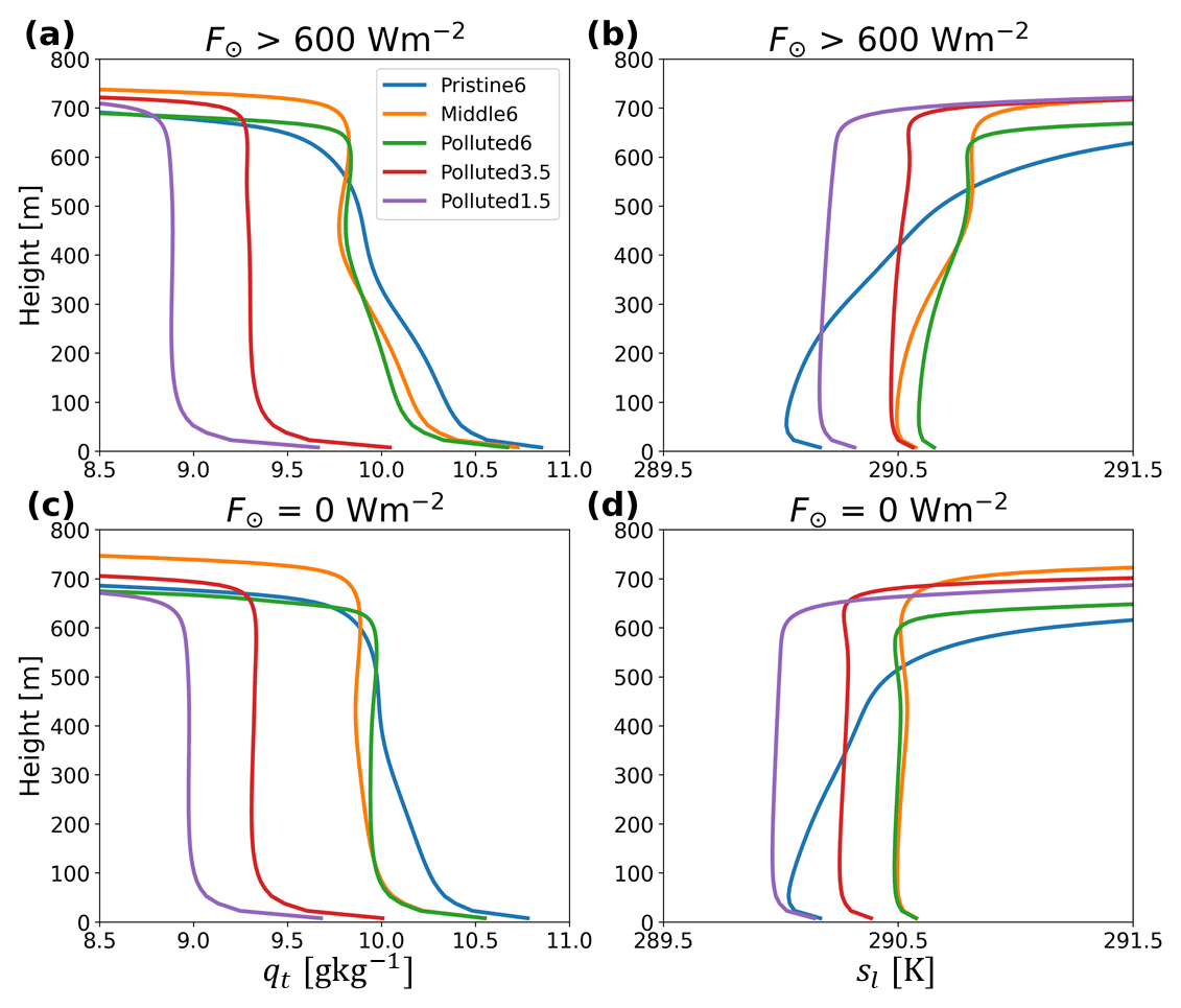
Figure 3Vertical profiles of (a, c) qt and (b, d) sl averaged during (a, b) day and (c, d) nighttime for the Ctrl case.
Figure 3 shows vertical profiles of qt and sl during day and nighttime. Generally, qt and sl profiles are more stratified during daytime than nighttime, as solar absorption at cloud top weakens the production of turbulence by longwave cooling. Evaporation of rain drops below cloud base stabilizes the MBL, so the Pristine6 case is the most stratified of the cases. The MBL is more stratified with a moister FT than a drier FT, as a drier FT is more transparent to outgoing longwave radiation so that cloud-top cooling is more effective.
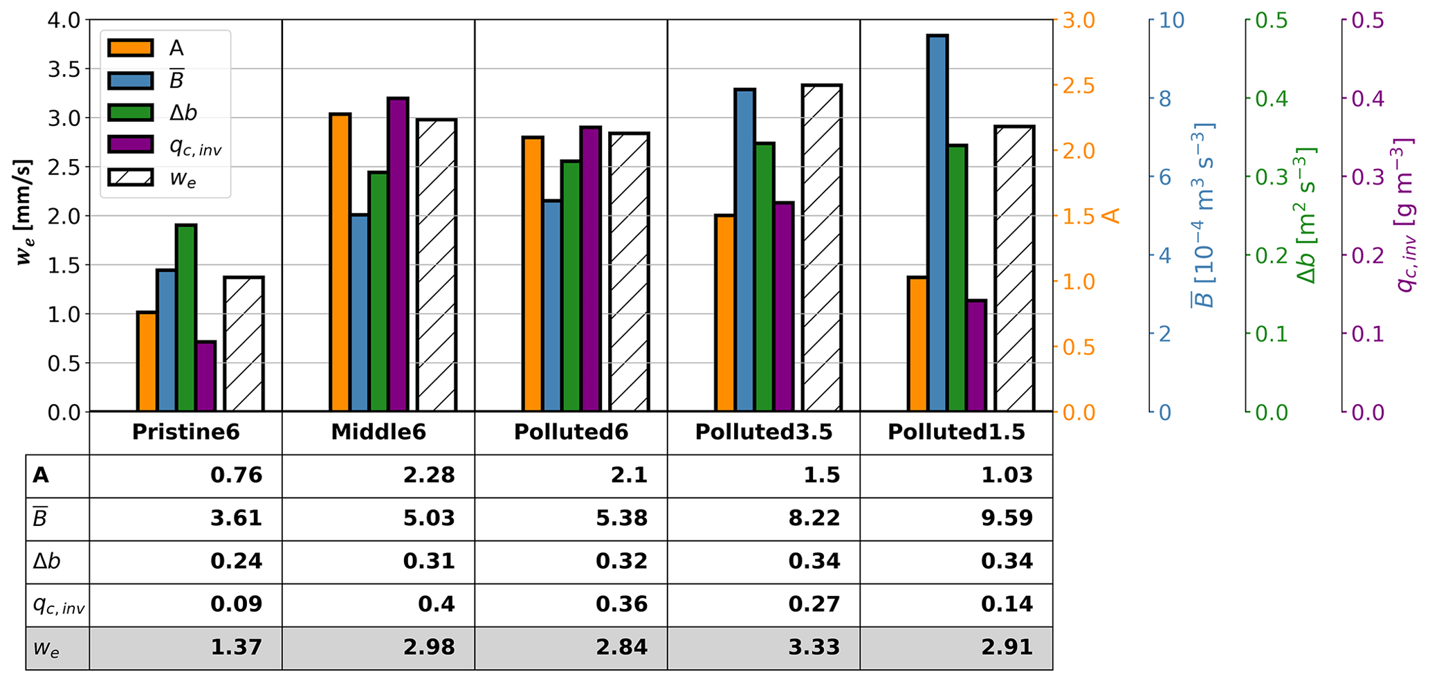
Figure 4Run-averaged entrainment velocity (we, hatching), entrainment efficiency (A, orange), boundary-layer-mean buoyancy flux (, blue), buoyancy jump (Δb, dark green), and cloud water mixing ratio at zinv−50 m (qc,inv, purple) in the Ctrl runs for the Pristine6, Middle6, Polluted6, Polluted3.5, and Polluted1.5 cases. The y axis on the left-hand side is for we, and the different colored axes on the right-hand side correspond to bars of the same colors in the figure.
The entrainment rate (we) also varies depending on meteorological conditions (Table 2, Fig. 4). Factors controlling we include boundary-layer turbulence, the strength of the buoyancy jump across the inversion Δb, the boundary-layer depth zinv, and an efficiency term A that incorporates the microphysical (e.g., evaporation and sedimentation) impacts on entrainment. We use the parametric formula suggested in Bretherton et al. (2007):
Here, w* is the convective velocity scale, a measure of the buoyant production of turbulence, defined as the vertical integral of the buoyancy flux over the boundary layer: . In this work, we define , as the vertical integral of buoyancy production normalized by the boundary-layer depth: . Therefore, Eq. (1) becomes
Thus,
As approximated by Eqs. (5) and (6) in Bretherton et al. (2007), entrainment efficiency (A) increases with entrainment-zone cloud liquid water amount, which is largely determined by sedimentation velocity and cloud thickness (Bretherton et al., 2007), and with the reduction in buoyancy due to evaporation by the dilution of cloud water with above-inversion air (e.g., Nicholls and Turton, 1986). The expressions in Eqs. (1) and (2) are approximate. If, for example, entrainment is related to a different metric of boundary-layer turbulence than (e.g., Stevens, 2002), the computation of A from simulated values of we, , and Δb will be affected. As a result, changes in A with aerosol perturbations may result from both changes in entrainment efficiency and errors in the approximations embedded in Eq. (3). Figure 4 shows run-averaged (after the spin-up) A, , Δb, cloud liquid water mixing ratio at zinv−50 m (qc,inv), and we in the Ctrl runs. Generally, A is proportional to qc,inv, consistent with the results of Bretherton et al. (2007).
In the Pristine6 Ctrl run, we is significantly weaker than the other runs, mainly due to small A and . The low A value may be attributed to low qc,inv caused by the high sedimentation velocity of large cloud droplets, whereas the low value is caused by the suppression of turbulence from rain formation, which warms the cloud layer, and precipitation evaporative cooling below cloud. Across the weakly precipitating and non-precipitating cases, we is quite similar, but the factors driving we are different. In the Middle6 and Polluted6 runs, where the FT is moist, A is high but is low. The high A value is mainly due to larger qc,inv, while the moist overlying FT leads to weaker cloud-top radiative cooling and low (e.g., Siems et al., 1990). For drier FTs, A and qc,inv decrease as clouds become thinner, but increases as cloud-top cooling becomes more effective. For all cases, we is greater at night than during the day, due to stronger net radiative cooling at cloud top. In the Pristine6 run, we at night (2.72 mm s−1) is 3 times greater than during the day (0.92 mm s−1). This is partly attributed to the large variation in the CF, in addition to the stronger net radiative cooling at night.
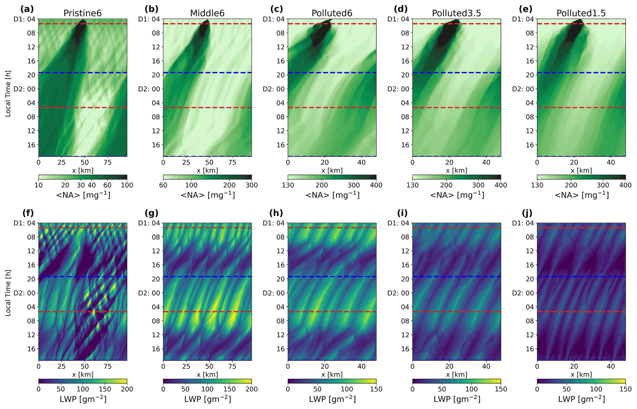
Figure 5Hovmöller plots of (a–e) 〈Na〉 and (f–j) the LWP in the Plume runs for the (a, f) Pristine6, (b, g) Middle6, (c, h) Polluted6, (d, i) Polluted3.5, and (e, j) Polluted1.5 cases across the 2 d simulation. Red and blue dashed lines indicate the times of sunrise and sunset, respectively.
3.1.2 Aerosol injection (Plume) runs
Figure 5 shows Hovmöller plots of the boundary-layer mean 〈Na〉 (Fig. 5a–e; hereafter, angled brackets represent the boundary-layer mean of a variable) and LWP (Fig. 5f–j) averaged along the y axis for the Plume runs for each case. For all of the cases, the ship tracks are approximately parallel to the roll axis, which strongly affects the lateral dilution of the plume (Berner et al., 2015). Except in the Pristine6 run, the plume edge tends to align with the mesoscale cell boundaries, showing that the mixing across the width of a cell is rapid, whereas the mixing to adjacent cells is relatively slow.
During Day 1 in the Pristine6 run, there is a fringe of clear sky at the edges of the plume (Fig. 5f), consistent with Wang and Feingold (2009) and Wang et al. (2011). These cloud-cleared regions are caused by a mesoscale circulation, generated by the gradient in precipitation rates between the region with a higher NCCLD, due to the injected plume, and the background. The widths of the cloud-cleared regions become broader up until the early afternoon, and they then narrow. At night, the roll structure develops within the plume, and the cloud-free fringes disappear. Clouds within the plume become overcast, while those in the background remain patchy but thick. On Day 2, the areas within the plume remain mostly overcast, while clouds in the background regions are more broken. Starting at sunrise on Day 2, 〈Na〉 in the background air starts to be depleted, likely because turbulence after sunrise is too weak to sustain the cloud number concentration against the loss by coalescence. In the other cases, there is no visible change in cloud morphology with aerosol injection.
Table 3As in Table 2 but for the differences between the Plume and Ctrl runs averaged across Day 1 (first row in each section), Night (second row in each section), and Day 2 (third row in each section).

3.2 Responses to aerosol injection
The impacts of aerosol injections are analyzed below using budget equations to quantitatively compare the roles of different processes in the Plume and Ctrl runs. Throughout, we use “d” in front of each variable to indicate the Plume − Ctrl difference. Comparisons are made for averages over Day 1, Night, and Day 2, respectively (Table 3). Values in square brackets indicate the standard deviation from the time series of the domain-mean differences and provide a measure of the robustness of the Plume − Ctrl differences.
3.2.1 Microphysical impacts on entrainment and turbulence
In all of the cases, the cloud droplet effective radius averaged over cloudy grids (re) robustly decreases with aerosol injection (Table 3), with stronger decreases when unperturbed re is large. The decrease in re is greatest in the Pristine6 case (−1.3, −1.7, and −1.6 µm for Day 1, Night, and Day 2, respectively), followed by the Middle6 case (−0.9, −0.9, and −1.6 µm) for Day 1, Night, and Day 2, respectively), despite lower aerosol injection rates in these runs. Among the three polluted cases, the re decrease is larger in the moister cases, as unperturbed re is larger; the increase in the Nc is very similar in all cases (Table 1).
In the Pristine6 and Middle6 cases, the cloud-base precipitation rate Rcb decreases in response to aerosol injection. Reduction in droplet size (Table 3) reduces collision–coalescence efficiency. dRcb in the Pristine6 case is −0.06, −0.26, and −0.04 mm d−1 for Day 1, Night, and Day 2, respectively; dRcb in the Middle6 case is −0.03, −0.07, and −0.06 mm d−1, respectively. The decrease is larger during nighttime and early morning because the background precipitation rate is higher. As there is negligible precipitation in the three polluted cases, dRcb is also negligible (Table 3). Likewise, Rsfc also decreases in the Pristine6 case (−0.02, −0.09, and −0.01 mm d−1 for Day 1, Night, and Day 2, respectively). Precipitation is too weak to reach the surface in the Middle6 case, so dRsfc∼0.
As a result of the reduction in re, the cloud-top entrainment rate we is enhanced in all cases due to the sedimentation–entrainment feedback (Table 3). Turbulence production through drizzle suppression (Wood, 2007) is more effective than the sedimentation–entrainment feedback with respect to enhancing turbulence (Bretherton et al., 2007), so dwe is greatest in the Pristine6 case (Table 3), where we in the Plume run is increased by 30 %–100 % over the Ctrl run. The increase in we in the Middle6 case is likely also aided by Rcb suppression. For the three polluted cases, dwe is weaker than in the two precipitating cases, but it generally increases with free-tropospheric moisture.
From Eq. (2), the relative change in entrainment rate can be expressed as
Run-averaged values of , , , and (Fig. 6) clearly show that entrainment efficiency changes (dA) dominate changes in entrainment. These changes are much greater in the Pristine6 case than in the Middle6 and three polluted cases (note the different axes), probably due to the greater reduction in re and, thus, also sedimentation velocity. Likewise, among the three polluted cases, is greater for a moister than a drier FT, which is also attributed to a greater reduction in re. Reduced turbulence (i.e., negative ) partly mitigates the A-driven increase in dwe. This is largely a damping of the MBL turbulence by the increased entrainment itself (Stevens, 2002), although in the Pristine6 case due to turbulence invigoration from precipitation suppression. is more negative in the Polluted6 case than in the Polluted3.5 case, likely because is greater, and the associated enhancement of entrainment results in increased stratification in the boundary layer.
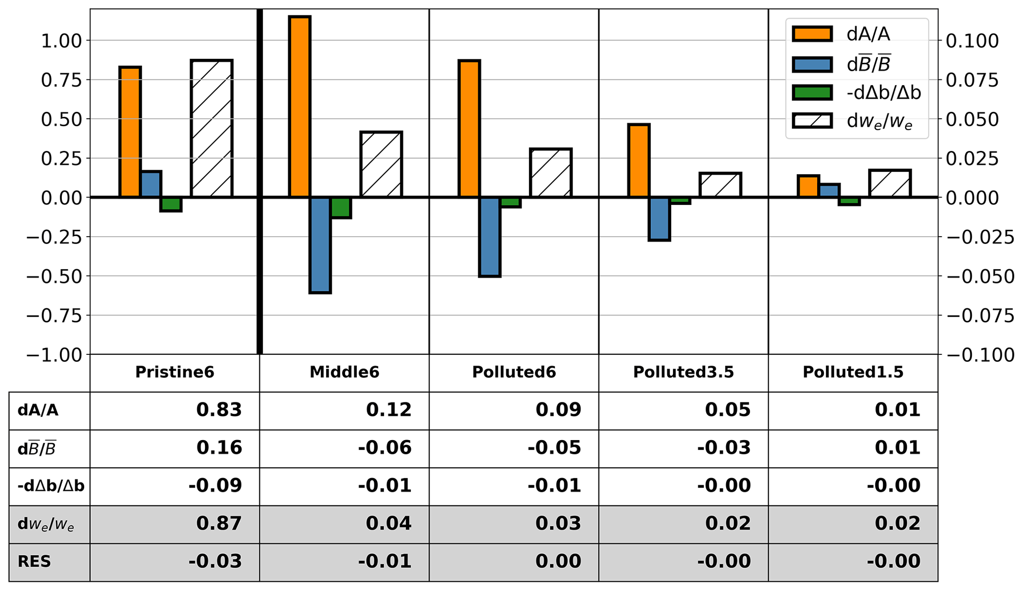
Figure 6Run-averaged fractional changes between the Plume and Ctrl runs of dwe (hatching), dA (orange), and (blue) and Δb (dark green) in the Pristine6, Middle6, Polluted6, Polluted3.5, and Polluted1.5 cases. Note that the y-axis scale for the Pristine6 case (left-hand side of plot) is 10 times greater than that for the other cases (right-hand side of plot). The table below the histograms shows the values of the fractional changes and the residual between fractional change in dwe as well as the sum of the rest of the values.
In contrast to the other polluted cases, in Polluted1.5 is positive. This is mainly attributed to greater cloud cover in the Plume run than in the Ctrl run (Table 3), leading to a stronger longwave radiative cooling and, thus, an intensification of turbulence. An increase in cloud thickness with greater entrainment can happen in a mixed layer (Randall, 1984) but typically requires a moist FT. Here, increased is occurring with an extremely dry FT, which one would expect to be detrimental to cloud amount. This behavior may be due to a response (increase) in surface fluxes, as discussed in the following section. Finally, it should be noted that contributes only weakly to dwe. In all cases, dΔb increases because stronger entrainment tends to sharpen the inversion.
These results imply that, in general, entrainment enhancement of weakly precipitating and non-precipitating MBLs is mainly caused by an increase in entrainment efficiency, which leads to stronger stratification of the boundary layer. In a precipitating MBL, although there is also a large increase in entrainment efficiency, buoyancy production by suppression of precipitation leads to a more turbulent boundary layer. The combination of the enhancement of A and drive a large enhancement of the entrainment rate.
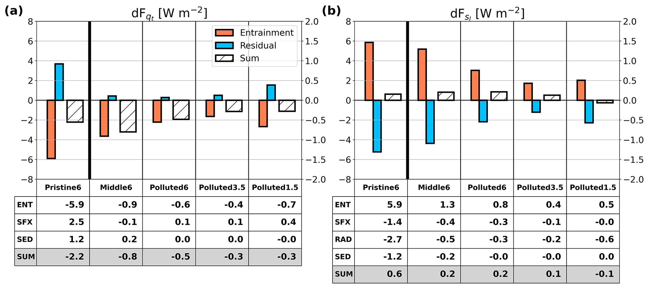
Figure 7(a) Run-averaged differences between the Plume and Ctrl runs in qt flux into the boundary layer by entrainment (orange) and the sum of the surface flux and surface precipitation (residual, blue). The hatched bars represent the sum of all of the fluxes. Panel (b) is the same as panel (a) but for sl. Residuals here include the fluxes induced by radiation responses. The tables below the histograms show the mean values for entrainment (ENT), surface fluxes (SFX), and radiation (RAD; for sl only) as well as their sum (SUM). Note the logarithmic y-axis scale.
3.2.2 Perturbations in qt and sl fluxes into the MBL by aerosol injections
As illustrated in Appendix A, LWP adjustments are controlled by changes in zinv and zcb, which are determined by both the mean and coupling state of qt and sl. In this subsection, we show the changes in the fluxes of qt and sl into the MBL in response to aerosol injections, which affect the MBL mean state. To understand the different responses of 〈qt〉 and 〈sl〉, perturbations in net fluxes of qt and sl into the boundary layer, averaged throughout the simulation ( and , respectively), are given in Fig. 7. Bars represent and by entrainment (orange), by the rest of the processes (blue), and the sum of all terms (hatched). The tables below the histograms in Fig. 7 show the net fluxes due to different processes (i.e., entrainment – ENT, surface flux – SFX, sedimentation – SED, radiation – RAD, and sum of all terms – SUM). The methods to calculate the net fluxes are given in Appendix A.
The change in fluxes from entrainment, and , in the Pristine6 case are −5.9 and 5.9 W m2, respectively, which are about 5–6 times greater than in the Middle6 case and about 1 order of magnitude greater than the in the polluted cases. Among the three polluted cases, is greatest for Polluted1.5, as Δqt is more negative for the drier FT. Because Δsl is comparable across all of these cases (Table 1), is mostly explained by dwe.
All of the other processes, such as the changes in the surface flux, sedimentation, and radiation, buffer the drying and warming of the boundary layer by entrainment enhancement. This buffering is most effective in the Pristine6 case, with surface moisture fluxes and precipitation suppression together offsetting almost two-thirds of the entrainment drying. Similarly, , , and together offset 84 % of the entrainment warming. The surface flux responses and the negative response are attributable both to changes in the MBL mean state and to changes in the degree of MBL coupling. The suppression of precipitation also induces moistening and cooling of the boundary layer (i.e., positive and negative , respectively). For the Pristine6 case, greater MBL cooling through the radiative flux response (i.e., negative ) is caused by an enhanced CF at night in the Plume run.
The buffering is less effective in the Middle6 case, where only 20 % of the entrainment drying is offset by a reduced precipitation flux, and the contribution from surface evaporation is negligible. Approximately 60 % of entrainment warming is buffered by a reduction in surface sensible heat flux, reduced precipitation warming, and increased radiative cooling. Although the MBL becomes drier, decoupling suppresses heat and momentum transport, inducing only weak damping from the surface fluxes. Moistening and cooling by precipitation suppression is less effective in the Middle6 case than in the Pristine6 case, due to weaker suppression of Rsfc. As dCF is negligible in the Middle6 case, the increased radiative flux divergence in this case is driven by reduced solar absorption from a reduced cloud LWP (Table 3).
The amount of buffering of entrainment drying by other responses depends on the free-tropospheric moisture. Of the polluted cases, is most negative for Polluted1.5 due to the drier FT. However, this drying is largely offset by so that is comparable to that in the Polluted3.5 case but weaker than that in the moister Polluted6 case. This can also be explained by the response of the coupling state of the MBL. The greater enhancement of entrainment in the moister FT induces greater stratification, making the damping by surface fluxes less effective.
, on the other hand, is more sensitive to 〈sl〉, rather than to stratification. is more negative in the Polluted6 case than in the Polluted3.5 case, probably because the greater decrease in the LWPCLD (e.g., Table 3) leads to a greater reduction in solar absorption. in the Polluted1.5 case is, however, much greater than in the Polluted6 and Polluted3.5 cases. This occurs because radiative cooling strengthens with a greater nighttime CF in the Plume than in the Ctrl run (Table 3).
These results imply that drying and warming of the MBL by entrainment enhancement is controlled not only by Δqt and Δsl but also by the response of the entrainment rate to aerosol perturbation. In addition, the surface fluxes, precipitation, and radiation respond to aerosol-induced changes in the MBL state and play important roles in the MBL qt and sl budgets. This suggests that studies of aerosol–cloud interactions of a day or longer should include interactive surface fluxes so that the buffering mechanisms seen here are represented.
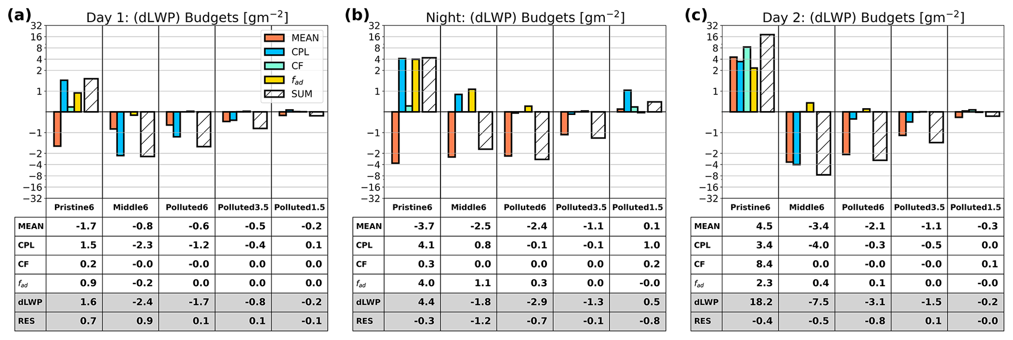
Figure 8The dLWP budgets for (a) Day 1, (b) Night, and (c) Day 2. The histograms show the dLWP induced by changes in the MBL mean state (orange) and coupling state (blue), the dLWP induced by changes in the CF (green) and fad (yellow), and the sum of all budget terms (SUM, hatched). The tables below the histograms show the values given in the plots as well as the residual between the actual dLWP and that estimated using the approach shown in Appendix. A. Note the logarithmic y-axis scale.
3.2.3 Cloud liquid water path adjustment
The previous sections showed how the mean value and MBL coupling state of qt and sl respond to aerosol injection as well as which processes contribute to the response. In this section, we analyze how changes in cloud and MBL properties affect cloud LWP adjustments. Here, we assume that changes in the domain-mean cloud liquid water are determined by changes in the cloud fraction (dLWPCF), cloud thickness (dLWPh), and cloud adiabaticity (). dLWPh is further decomposed into contributions to dLWP via changes in cloud thickness resulting from a response in the MBL mean state (dLWPMEAN) and in the degree of MBL coupling (dLWPCPL). Based on this, cloud LWP adjustments can be decomposed as follows:
Details on how each term is calculated are given in Appendix A. Bars in Fig. 8 show dLWP caused by changes in the cloud thickness from responses in the MBL mean state and the coupling state, changes in the CF, and changes in adiabaticity as well as the sum of all of the terms during (Fig. 8a) Day 1, (Fig. 8b) Night, and (Fig. 8c) Day 2.
On Day 1, dLWPMEAN is negative in all cases and is most negative for the Pristine6 case, followed by the Middle6, Polluted6, Polluted3.5, and Polluted1.5 cases. This is consistent with the degree of entrainment enhancement across the cases, indicating that MBL warming and drying by aerosol injection are mainly driven by entrainment enhancement. At Night, dLWPMEAN becomes more negative, except in the Polluted1.5 case. This implies that the system continues to move toward a drier and warmer steady state, which is consistent with the results of the Glassmeier et al. (2021) simulations, which showed that the adjustment equilibrium timescale of cloud macrophysics (about 1 d) is much longer than that of the cloud microphysics (5–10 min).
On Day 2, dLWPMEAN in the Pristine6 case becomes positive (4.66 g m−2). This sign change in dLWPMEAN is mainly attributed to greater nocturnal drizzle suppression. Drizzle suppression is ineffective during daytime, as background Rcb is weak (e.g., Table 2). Therefore, entrainment drying and warming are stronger than the damping effects discussed above. At night, drizzle starts to be strongly suppressed (e.g., Table 3), leading to significant liquid water retention and turbulence generation. Thus, dLWP is driven more strongly by changes in sedimentation (i.e., surface precipitation), surface fluxes, and radiation during night. As a result, by the end of the night period, entrainment drying and warming is more than offset by these responses, leading to more positive dLWP. Accumulated drizzle suppression during nighttime leads to significant positive dLWPMEAN on Day 2. This leads not only to thicker clouds but also to a greater CF. During Day 1 and at night, dLWPCF is negligible (0.26 and 0.29 g m−2, respectively). On Day 2, dLWPCF becomes 8.44 g m−2, and this term dominates dLWP. Without significant suppression of precipitation, the weakly precipitating and non-precipitating cases do not have this sign change in dLWPMEAN.
Changes in the MBL coupling state in response to aerosol injection also have significant impacts on dLWP. Because turbulence in the MBL is intensified by drizzle suppression, dLWPCPL is positive in the Pristine6 case. More precipitation is suppressed at night, making dLWPCPL more positive at night than during daytime. During daytime in the Middle6, Polluted6, and Polluted3.5 cases, dLWPCPL is negative due to increased stratification of the boundary layer. dLWPCPL tends to be more negative during daytime when the background clouds are thick (Table 2), due to a significant enhancement of the entrainment efficiency (i.e., Fig. 4) leading to greater stratification. At night, however, dLWPCPL in these cases becomes negligible, as background drizzle is intensified. In the Polluted1.5 case, where the background LWP is very low, dLWPCPL is negligible during daytime. At night it becomes positive, and this term dominates total cloud LWP changes.
In the Pristine6 and Middle6 cases, where Rcb is not negligible, aerosol-induced Rcb suppression reduces the loss of cloud liquid water by drizzle, leading to an increase in the adiabaticity of MBL clouds (Wood, 2005). However, as there is no precipitation in the polluted cases, there is, of course, no reduction in Rcb (Table 2), and is insignificant.
The overall LWP adjustment dLWPSUM in the Pristine6 case is positive, despite significant enhancement of we, due to responses in the coupling state of the MBL by precipitation suppression and the increase in the CF and fad offsetting entrainment drying. dLWPSUM increases with time, as drizzle suppression is accumulated. dLWPSUM during daytime in the Middle6 case, where the background LWP is greatest, is the most negative of all of the cases and becomes less negative as the background LWP decreases. dLWPSUM is more negative on Day 2 than on Day 1 in the weakly precipitating and non-precipitating MBLs (i.e., all cases other than Pristine6). The Middle6 case stands out as having a relatively smaller negative dLWPSUM at night than during either of the days, compared with the other cases. This is because the background Rcb in this case is larger so that positive values of dLWPCPL and compensate for the negative dLWPMEAN. In the Polluted1.5 case, where the background clouds are quite thin, the LWP adjustment is much weaker.
3.2.4 Aerosol and cloud number concentration
The lifetime of aerosol perturbations is an important factor for determining the full extent of cloud radiative responses to an injection event. The temporal evolution of the aerosol perturbations is analyzed by separating the changes in the total aerosol within the boundary layer (d〈Na〉) into contributions from different processes: entrainment (ENT), autoconversion (AUT), accretion (ACC), scavenging (SCV), sedimentation (SED), and surface flux (SFX). Tendencies of 〈Na〉 for AUT, ACC, SCV, SED, and SFX are calculated online (as illustrated in Sect. 2.2), whereas the tendency of 〈Na〉 for ENT is estimated using , where Na(z) is the total aerosol number concentration at level z. The contributions to d〈Na〉 by the end of the simulation are calculated as the difference in each tendency term between the Plume and Ctrl runs, integrated over the time of the simulation. Figure 9 shows , i.e., the contribution to from the different processes. For example, a unit of −1 cm−3 cm3 means that the initial perturbation has dissipated completely over the time of the simulation (39.5 h), whereas +1 cm−3 cm3 means the initial aerosol perturbation has doubled. Figure S5 in Supplement shows that the budget calculations agree well with the evolution of 〈Na〉.
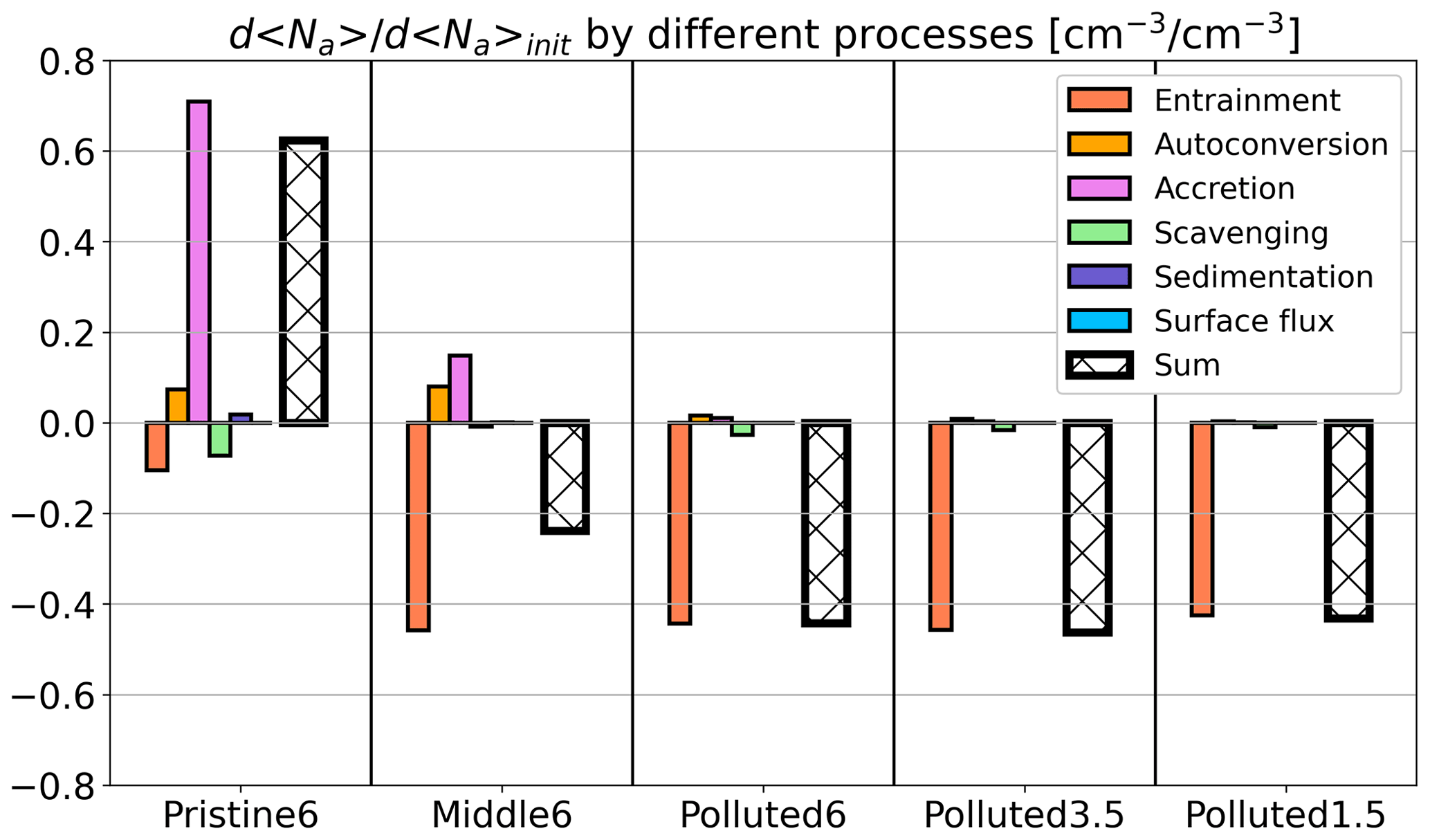
Figure 9Fractional changes in the initial Na perturbation resulting from different microphysical responses to aerosol injection, averaged across the 2 d simulation: entrainment (red), autoconversion (orange), accretion (magenta), scavenging (green), and surface flux (blue). The thick hatched bars represent the sum of all of the budget terms.
Because the aerosol injections increase 〈Na〉 considerably, dilution by cleaner free-tropospheric air acts as a sink and negative d〈Na〉. is smaller in the Pristine6 case than in the other cases (about −0.1 cm−3 cm3). This is mainly because the FT is more polluted than the boundary layer, and the initial perturbation is not significant compared with the jump in Na across the inversion (see Table 1). In the other cases, where the boundary layer is more polluted than the FT, acts as a major sink, ranging from −0.45 to −0.47 cm−3 cm3.
Another primary cause of differences in across cases is collision–coalescence. For precipitating clouds, aerosol injections reduce coalescence scavenging, so that the sink of aerosol to accretion and autoconversion decreases. In the Pristine6 case, where precipitation is most strongly suppressed, accretion and autoconversion decreases together induce positive (contributing 0.70 and 0.07 cm−3 cm3, respectively). This implies that, in a strongly precipitating MBL, aerosol injection may induce a transition from open to closed cells. In a weakly precipitating case (Middle6), due to change in accretion and autoconversion is positive but smaller (0.07 and 0.12 cm−3 cm3, respectively), extending the lifetime of the aerosol perturbation. In non-precipitating cases, these effects are negligible.
Scavenging of aerosol by coagulation onto cloud droplets induces universally negative , as the higher concentration of Na produced by aerosol injection leads to a higher scavenging rate. However, these terms do not have a large impact in the overall in any of the cases examined. Surface aerosol fluxes and sedimentation of rain and cloud droplets do not respond significantly to aerosol injection, so this does not contribute to .
Based on the budget approach presented here, we can infer the lifetime of aerosol perturbations. The sum of all of the terms (hatched bars in Fig. 9, ) represents the change in over the duration of the experiment after injection (39.5 h). Thus, the lifetime can be roughly estimated by dividing 39.5 h by . As increases with time for the Pristine6 case, it is not possible to estimate a lifetime for injected aerosol in this case. The injected aerosol lifetime in the Middle6 case is ∼90 h; for the polluted cases, it is ∼65 h. These timescales are considerably larger than the typical age (∼7 h) of ship tracks detected using satellite observations (Durkee et al., 2000). Coupled with the fact that the magnitude of the cloud LWP adjustments becomes stronger on Day 2 than on Day 1 (Fig. 8), this points to the need to track cloud responses to aerosol injections over multiple days in order to provide an assessment of their overall radiative effect. After 2 d, most ship tracks will have lost their identity, and it may be difficult to distinguish regions containing injected aerosol from marine background conditions.
3.2.5 Cloud radiative effect
Previous sections have illustrated how the cloud LWP and cloud droplet number concentrations respond to aerosol injections for the different background meteorological and aerosol cases. This section analyzes injection-induced changes in the cloud radiative effect (dCRE) by decomposition into contributions from changes in the Nc (), i.e., the Twomey effect, and from those due to adjustments in the cloud LWP (dCRELWP) and CF (dCRECF). The decomposition approach is described in Appendix B. In all of the cases, the residuals (RES) between the actual dCRE and the sum of all components are much smaller than individual components, indicating that the decomposition works quite well. The values of dCRE given here are an average over 24 h, so the zero values during nighttime are accounted for. When comparing dCRE across cases, it should be noted that the domain size in the Pristine6 and Middle6 cases is twice that of the polluted cases and that the amount of aerosol injection is different among the cases (see Table 1). The bar plot in Fig. 10 summarizes , dCRELWP, and dCRECF on Day 1 and Day 2 for all of the cases.
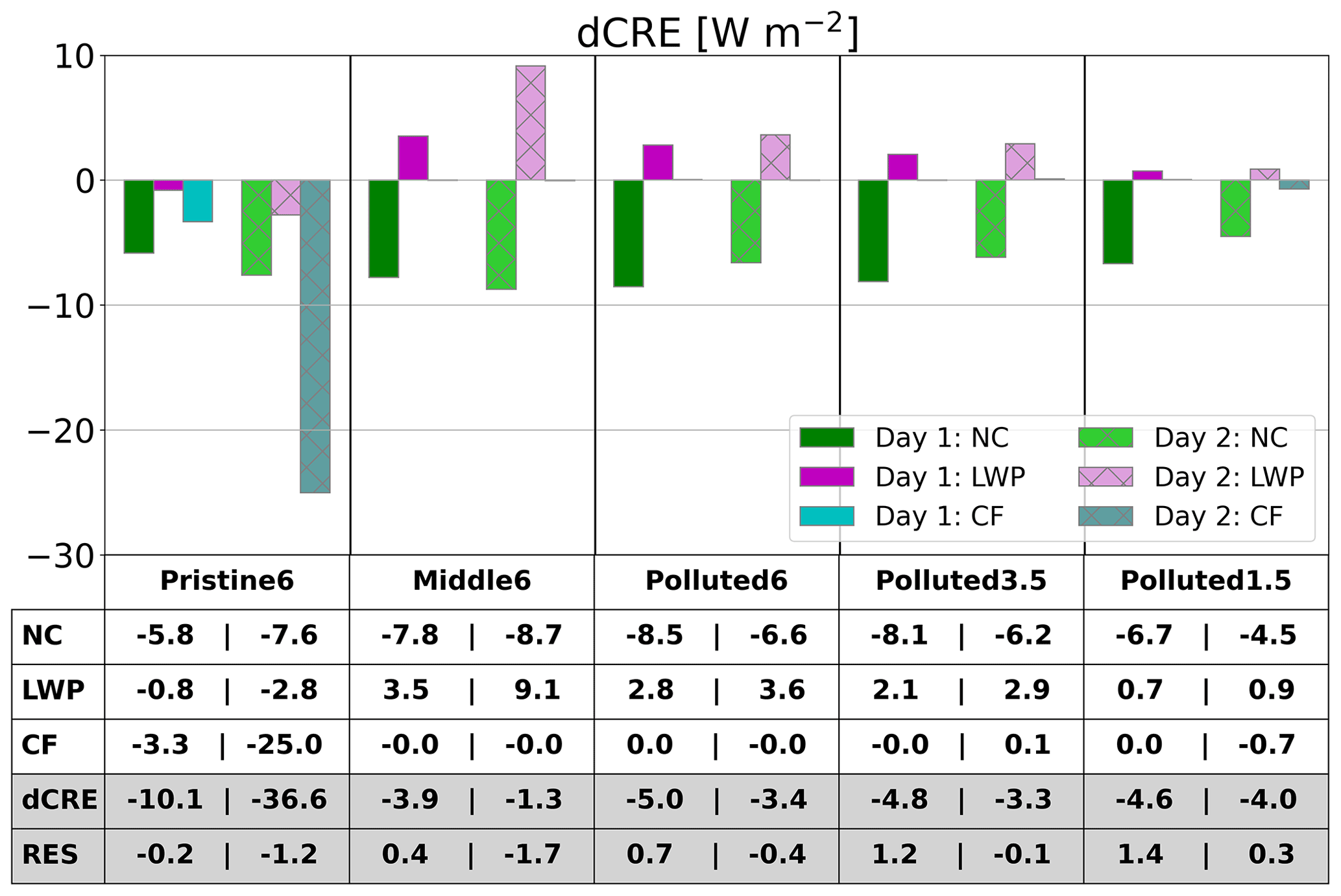
Figure 10The difference in the decomposed 24 h cloud radiative effect between the Plume and Ctrl runs (dCRE) for each case, showing contributions from (green), dCRELWP (magenta), and dCRECF (blue). The darker colors show the average dCRE for Day 1, and the lighter colors with hatching show the averages for Day 2. The table below the histograms shows , dCRELWP, dCRECF, dCRE, and the residual between the actual dCRE and that estimated using an approach shown in Appendix B for Day 1 (left bars) and Day 2 (right bars).
For the Pristine6 case, , dCRELWP, and dCRECF on Day 1 are −5.8 and −0.8, and −3.3 W m−2, respectively. Positive adjustments in both the LWPCLD and CF (Table 3) approximately double the brightening induced by the Twomey effect alone. On Day 2, contributions from all three cloud properties increase in magnitude (Fig. 10), with dCRECF dominating the brightening.
For all other cases, the cloud fraction responses dCRECF contribute only minimally or not at all to dCRE, and CRE changes largely comprise Twomey effects and LWP adjustments only. In all cases other than the Pristine6 case, LWP adjustments are negative (dCRELWP>0). In the Middle6 case, LWP reductions offset almost 50 % of Twomey brightening on Day 1. On Day 2, there is a small amount of cloud brightening in the morning, but there is darkening during the afternoon that offsets the cloud brightening earlier in the morning (Fig. S7b). The actual dCRE during Day 2 of Middle6 indicates brightening, even though the sum of the Nc, LWP, and CF contributions to dCRE indicates darkening. This discrepancy is attributed to the near cancellation of the Nc and LWP contributions, which allows errors in predicting the individual contributions to dominate the total. For the three polluted cases, is similar across cases, and it is slightly smaller on Day 2 than on Day 1 in all cases. Although a more evenly distributed plume would result in greater Twomey brightening on Day 2, this is offset by the fact that the magnitude of the aerosol perturbation is decreasing with time (Fig. 9). The negative LWP adjustments in the polluted cases offset 10 %–30 % of the Twomey effect on Day 1; this increased to 20 %–50 % on Day 2. It is noteworthy that dCRELWP is more positive under a moist FT (Fig. 10), a response that appears to differ from Glassmeier et al. (2021), wherein the strongest negative LWP adjustments occur with a very dry FT. This is due to the greater entrainment enhancement under a moist FT, leading to more significant stratification and a weaker surface flux response than under a dry FT, as described above in earlier sections.
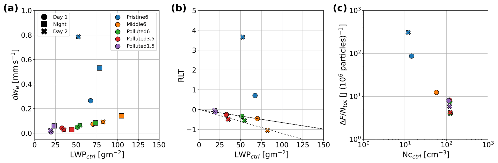
Figure 11(a) Sensitivity of dwe to the LWPctrl. The circle, square, and cross markers represent Day 1, Night, and Day 2 averages, respectively. Panel (b) is the same as (a) but for the sensitivity of RLT to the LWPctrl. (c) Sensitivity of brightening efficiency (i.e., the radiative forcing per 106 particles) to Nc,ctrl.
Our results highlight the complexity of cloud responses to aerosol injections. Changes in the mean state and the coupling state of the MBL, changes in cloud cover, and changes in the adiabaticity of MBL clouds (Fig. 8) are important for determining the cloud radiative responses. Cloud responses depend on the background conditions, such as background aerosol loading, cloud thickness and cover, and free-tropospheric moisture. A key result is that the aerosol-induced increases in the cloud-top entrainment rate are more rapid for thicker than for thinner clouds (Fig. 11a) because entrainment efficiency, which is an estimate of how strong entrainment is for a given level of turbulence, is more strongly affected by cloud thickness (Hoffmann et al., 2020; Zhang et al., 2022) than by the dryness of the FT. In weakly precipitating and non-precipitating MBLs (i.e., the Middle6, Polluted6, Polluted3.5, and Polluted1.5 cases), entrainment enhancement (dwe) monotonically increases with an unperturbed background LWP (Fig. 11a). This result seems to be broadly consistent with Possner et al. (2020), who show that the LWP susceptibility to the cloud number concentration is more negative when the boundary layer is deeper and, thus, clouds are thicker. In a strongly precipitating MBL (e.g., the Pristine6 case here), turbulent intensification by suppression of drizzle evaporation greatly augments the increase in entrainment efficiency. In response to enhanced entrainment, perturbations in surface fluxes, radiative fluxes at cloud top, and precipitation all offset entrainment-enhanced drying and warming of the MBL. In addition, changes in MBL stratification (quantified here as changes in coupling, cloud cover, and adiabaticity) by entrainment enhancement (drizzle suppression) also affect cloud macrophysics and, thus, cloud radiative properties.
Figure 11b shows the impact of the background LWP on the ratio of the radiative effects of cloud adjustments (the LWP and CF) to the Twomey effect (i.e., RLT = (). For example, RLT indicates that the Twomey effect is exactly canceled by cloud adjustments, whereas RLT indicates that the adjustments produce a doubling of the brightening compared with the Twomey effect alone. For weakly precipitating and non-precipitating MBLs, RLT tends to linearly decrease with the background LWP (Fig. 11b). On Day 2, the slope of the line becomes more negative, as the system moves toward an equilibrium steady state (Glassmeier et al., 2021). The regression lines imply that cloud darkening occurs when the LWP is greater than 150 g m−2 on Day 1 and 80 g m−2 on Day 2, which is much higher than the 55 g m−2 estimated from satellite observations over the northeastern Pacific (Zhang et al., 2022). Despite the discrepancy, our results seem to be consistent with satellite observations from (Zhang et al., 2022) in that the observations are obtained at ∼ 13:30 LT (local time) when clouds become thin and negative LWP adjustment becomes most significant due to diurnal variation (see Figs. S2 and S7). In the strongly precipitating Pristine6 case, the LWP adjustment becomes more positive, so that RLT becomes positive.
One can define a brightening efficiency as the total additional solar energy reflected per injected particle. The per-particle efficiency decreases by over an order of magnitude as the background Nc increases from 10 to 100 cm−3 (Fig. 11c). This is consistent with results from other LES studies and is somewhat steeper than that from a simple heuristic model with no cloud adjustments (see Fig. 4d in Wood, 2021). Positive LWP adjustment at low Nc and negative adjustments under more polluted conditions steepen this curve compared with expectations from the Twomey effect alone. This nonlinearity means that assessments of the potential global forcing from MCB (e.g., Wood, 2021) should ideally consider the temporal variability in the background cloud droplet concentration and aerosol. Such a strong sensitivity of the brightening to the unperturbed aerosol state also suggests that there may be considerable benefit in targeting injections to occur primarily in regimes with very low aerosol concentrations. These regimes of extreme albedo susceptibility likely occur relatively infrequently, but they could provide a significant fraction of the overall MCB radiative forcing. However, rare extreme brightening events likely make it challenging to assess MCB efficacy for a region as a whole.
The lifetime of aerosol perturbations is also examined here, as this will directly impact the duration of cloud radiative effects. In strongly drizzling MBLs, aerosol injection significantly reduces coalescence scavenging losses by cloud and rain drops, enough to surpass the enhanced loss by entrainment dilution (Fig. 9). This leads to increasing aerosol and cloud number concentrations in the MBL, at least over the first 2 d, making it impossible to define an injected aerosol lifetime. Even in a weakly drizzling MBL, aerosol lifetime can be extended by slowing the rate at which the aerosol perturbation is damped. Our simulations show that the aerosol lifetime in a non-precipitating MBL, which is mainly determined by entrainment dilution, is about 65 h, which is much longer than the typical longevity of ship tracks seen in satellite observations (e.g., Durkee et al., 2000; Gryspeerdt et al., 2021). One possible reason for this is that ship track identification using satellite images is essentially based on the variation in the cloud number concentration over the track, which sharply decreases with time, mainly due to lateral dilution (plume dispersion) (Berner et al., 2015) rather than losses by microphysical processes. As the aerosol plume spreads and dilutes, such aerosol perturbations will become more difficult to detect above the noise caused by spatial variability in background clouds. A lack of track detectability does not necessarily mean a lack of radiative forcing, however. More work is required to understand how satellite observations can be used together with LES to assess track detectability and radiative forcing for those cases where the injected aerosol had spread and diluted markedly. Aerosol lifetime might also depend on the jump in the aerosol number concentration across the inversion, which is not a focus of this study. However, given the small increase in the cloud-top entrainment rate with aerosol perturbation in non-precipitating MBLs (i.e., 2 %–5 %; shown in Fig. 6), the jump in the aerosol number concentration might have a marginal impact on the lifetime.
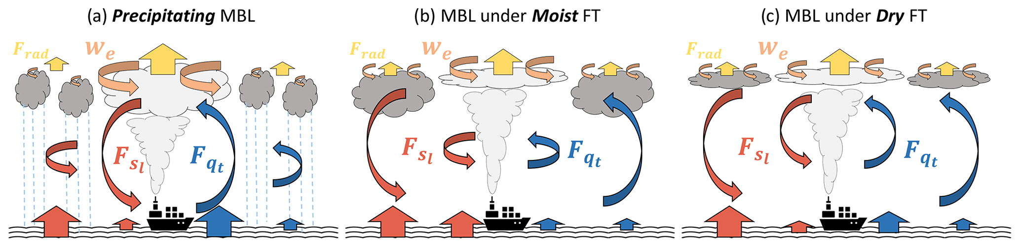
Figure 12This schematic illustrates the responses of the entrainment rate (light red arrows), boundary-layer turbulence (curved arrows in the boundary layer), surface fluxes (arrows on the surface), and cloud radiative fluxes (yellow arrows on the top of clouds) to aerosol injections. Red arrows represent sensible heat flux, and blue arrows represent moisture flux. The size of the arrows represents the intensity. The center of the domain is the region perturbed by ship tracks; to the left and right of this are the unperturbed regions. Response tendencies are shown for three sets of MBL conditions: (a) precipitating boundary layer, (b) non-precipitating MBL under a moist FT, and (c) non-precipitating MBL under a dry FT.
Figure 12 conceptualizes the findings in this study. It illustrates the responses in precipitation, entrainment rate, boundary-layer turbulence, and surface fluxes to aerosol injection under different meteorological conditions. In a strongly drizzling MBL (Fig. 12a), drizzle is strongly suppressed by aerosol injection. This induces a large enhancement of the entrainment rate, both by increased entrainment efficiency and by turbulent invigoration. As a result, there is considerable entrainment drying and warming of the MBL. However, these effects are largely countered by other processes. First, turbulent invigoration by suppressed subcloud precipitation evaporation and greater retention of cloud liquid water in the cloud both drive better MBL coupling. In addition, drying and warming of the MBL are largely offset by negative surface sensible and latent heat flux feedbacks, reduced moisture loss from surface precipitation, and increased longwave radiative flux divergence. The combination of these effects results in large increases in cloud thickness, cover, and adiabaticity, further enhancing brightening from the Twomey effect.
The responses of clouds in weakly precipitating and non-precipitating MBLs are distinctly different. In these cases, the entrainment rate is enhanced by the cloud droplet sedimentation–entrainment feedback. Because drizzle suppression is weak or negligible, it provides no source of turbulent invigoration. Instead, MBL turbulence tends to weaken in response to aerosol injections because enhanced entrainment reduces the buoyancy flux (Stevens, 2002). This leads to increased MBL decoupling. In addition, weaker turbulence makes surface flux moistening/cooling feedbacks less effective. Therefore, a combination of entrainment drying/warming and increased MBL stratification makes clouds thinner, reducing the cloud LWP. Figure 12b and c illustrate the steady-state adjustment of clouds to aerosol injection under moist and dry free-tropospheric conditions, respectively. Under a moister FT without strong drizzle (Fig. 12b), background clouds are thick. Aerosol injection into thick clouds considerably enhances the entrainment rate. Without the strong damping effect of surface fluxes, the MBL becomes drier and warmer. Furthermore, the MBL is more stratified, leading to weaker moisture and temperature fluxes through cloud base and, thus, greater cloud thinning. Under a dry FT (Fig. 12c), on the other hand, background clouds are thin and the sedimentation–evaporation feedback in thin clouds leads to a weaker enhancement of entrainment. This leads to weak drying/warming of the boundary layer, little induced stratification, and, thus, only a small reduction in cloud thickness.
These results are in contrast with previous observational (e.g., Gryspeerdt et al., 2019; Possner et al., 2020) and modeling (e.g., Wood, 2007; Glassmeier et al., 2021) studies, where increasing aerosol concentrations in clouds with a dry overlying lower FT induce a large reduction in the cloud LWP. This difference might be because our simulations are for a specific regime of stratocumulus clouds – those in a shallow and mostly coupled MBL. The LWP increases more rapidly with MBL depth under a dry FT due to more effective cloud-top cooling; thus, mixing (e.g., Eastman and Wood, 2018; Possner et al., 2020) and negative LWP adjustment under a dry FT might become more negative rapidly with MBL depth compared with that under a moist FT. A recent modeling study by Glassmeier et al. (2021) found that the Twomey effect could be entirely canceled by negative LWP adjustments (cloud thinning) in an extremely dry FT, leading to low radiative forcing or even cloud darkening. That study noted that the timescale of cloud macrophysics (about 20 h) is much longer than that of the cloud microphysical response to aerosol perturbation (less than 1 h). As such, Glassmeier et al. (2021) concluded that the radiative forcing derived for ship tracks, which are mostly observed only a few hours after injection, may represent an overestimate of the overall cooling effect of the ship track, as it misses the negative LWP adjustments that affect the clouds over several days. However, their simulations used fixed latent and sensible heat fluxes from the ocean surface, which we find to be one of the main processes that offsets the drying and warming of the MBL by enhanced entrainment. As the timescale of these damping effects is comparable to that of cloud macrophysics, the strength of negative LWP adjustments in a steady-state equilibrium may be overestimated in Glassmeier et al. (2021).
Future work should investigate other cloud regimes, such as deeper, more decoupled MBLs with cumulus under stratocumulus, using high-resolution, process-resolving models. Our simulations only cover shallow, well-mixed stratocumulus cloud, which is not the most dominant low-cloud regime over the subtropical and tropical oceans. Thus, in order to reduce uncertainty in the global cloud radiative forcing caused by anthropogenic aerosol emissions and to evaluate the potential efficacy of MCB, we also need to quantify the processes occurring in different MBL regimes. It is expected that the balance of processes described here will differ in other cloud regimes.
Our limited understanding of aerosol–cloud interactions accounts for a considerable uncertainty in anthropogenic aerosol radiative forcing. In an attempt to overcome challenges associated with entangled aerosol and meteorological influences on clouds (Stevens and Feingold, 2009), many studies have utilized “natural experiments” such as ship tracks and cloud responses to emissions from volcanic eruptions and power plants (Christensen et al., 2021). These real-world aerosol-induced cloud responses have provided invaluable insights into aerosol–cloud interactions, as we can directly compare the cloud properties with and without aerosol perturbations under the same meteorological conditions. However, these studies show a large variability in responses, implying that cloud responses are strongly dependent on the meteorological conditions as well as on the background and injected aerosol properties. This motivates the investigation of aerosol–cloud interactions under a variety of meteorological conditions using LES modeling.
This study investigates the MBL and cloud responses to aerosol injections in LES runs in a shallow, idealized stratocumulus-topped MBL near the Californian coast (35∘ N, 125∘ W). We focus on the effects of different background aerosol loading and levels of free-tropospheric moisture, using 2 d simulations of five cases with different background aerosol number concentrations, free-tropospheric moisture, and large-scale subsidence. Across 2 d of simulation, a case with a clean MBL and three cases with polluted MBLs under different lower FT (1.5–6.0 g kg−1) showed cloud brightening and cloud radiative effects ranging from −3 to −35 W m−2 across the cases and simulation days. A moderately polluted case with higher free-tropospheric moisture (6 g kg−1) had cloud brightening on Day 1 and Day 2 in the morning and cloud darkening in the afternoon on Day 2, which canceled almost all of the brightening in the morning on Day 2. The relative contribution of cloud adjustments to the Twomey effect (RLT; Fig. 11b) ranges from −1 to 4, which is consistent with estimates from various observations (e.g., Hu et al., 2021; Zhang et al., 2022).
Our results show that aerosol injection affects the cloud-top entrainment rate, MBL turbulence, surface fluxes, and cloud microphysics differently depending on meteorological conditions. These responses alter the mean and coupling states of the MBL, which both play important roles in the cloud adjustment.
The followings are the key responses modulating the LWP adjustment:
-
Aerosol injection enhances the cloud-top entrainment rate through the sedimentation–entrainment feedback (Bretherton et al., 2007). This enhancement is larger when the unperturbed clouds are thick, as the cloud drop size is then more susceptible to aerosol perturbation, leading to increased entrainment efficiency. In precipitating conditions, suppression of cloud-base precipitation greatly enhances the entrainment rate (Bretherton et al., 2007).
-
Enhanced entrainment induces MBL drying and warming, which is substantially damped by perturbations in surface latent and sensible heat fluxes, by radiative flux at cloud top, and by surface precipitation. The damping effect by surface fluxes is more effective when the boundary layer is well mixed. When drizzle is greatly suppressed, increased cloud cover (which increases radiative cooling) and increasing cloud adiabaticity both augment the damping.
-
The response of the MBL coupling state to aerosol injection strongly depends on the background meteorological conditions. In a strongly precipitating MBL, the suppression of subcloud drizzle evaporation induces stronger coupling of the MBL, leading to an increased cloud amount and LWP. In weakly precipitating and non-precipitating MBLs, aerosol injections cause stronger MBL stratification by entraining more buoyant air from the FT; this leads to a decreased cloud LWP. The greater entrainment enhancement is, the more stratified the MBL becomes. The stratification effect is shown to be more significant during daytime than at nighttime.
-
In a strongly precipitating MBL, precipitation suppression significantly reduces aerosol loss by coalescence scavenging, causing differences in aerosol concentrations between the runs with (Plume) and without (Control) aerosol injections to increase with time over the 2 d simulation. This implies an infinite effective lifetime for injected aerosol. The effective aerosol lifetime in non-precipitating MBLs is estimated at 65 h; this is much longer than the estimates of ship track lifetimes made using satellite images (e.g., Durkee et al., 2000; Gryspeerdt et al., 2021). Even a weak suppression of precipitation significantly extends the effective lifetime of aerosol perturbations.
-
In all cases examined, aerosol injections into shallow marine clouds induce Twomey brightening, augmented by the positive LWP adjustment in a pristine MBL with strong drizzle and offset by negative LWP adjustments in moderate and polluted MBLs. Twomey brightening is more strongly offset by negative LWP adjustments when the FT is moister. Clouds in a strongly precipitating MBL become brighter with time following aerosol injection, whereas the brightening in weakly precipitating and non-precipitating MBLs decrease on Day 2 of simulation. It is, therefore, possible that there could be cloud darkening beyond the 2 d duration of our simulations, which is an issue requiring further exploration.
Given the multiday effective lifetime of injected aerosol and the finding that the cloud LWP responses (be they positive or negative) grow with time, we may conclude that even 2 d simulations are not of a sufficient duration to fully capture marine low-cloud responses to point-source aerosol injections. In reality, meteorological boundary conditions will not be constant for such long periods; thus, a future simulation strategy is required that allows for quasi-idealized evolution of boundary conditions (e.g., increasing sea surface temperature (SST) over time). Such simulations will more realistically capture the evolution of background cloud fields over the subtropical eastern oceans.
Mixed-layer theory, first proposed by Lilly (1968), has been widely used to model stratocumulus-topped boundary layers, and it is a simple but useful tool to investigate microphysical and macrophysical processes controlling cloud thickness (e.g., Randall et al., 1984; Wood, 2007; Hoffmann et al., 2020). However, the fundamental assumption in the mixed-layer model that the boundary layer is fully mixed and liquid water adiabatically increases with height without consideration of cloud cover is not an accurate portrayal of reality in many cases. Here, we use a modified model that predicts the LWP responses to changes in cloud thickness and cover as well as the adiabaticity of clouds as follows:
Here, is the lapse rate of the liquid water content, zinv is inversion height, fad is adiabaticity, and h is cloud thickness. fad is calculated as an average of adiabaticity at every cloudy column. For the calculation of adiabaticity for individual cloudy columns, cloud thickness h is defined as a vertical thickness of grids where the Nc is greater than 0.1 cm−3. Assuming that the aerosol perturbation changes h, CF, and fad, the resulting adjustment of the LWP can be expressed as follows:
where d represents the difference between the Plume and Ctrl runs.
The LWP adjustment due to changes in cloud thickness LWPh can be further decomposed because cloud thickness adjustments arise from changes in both zinv and zcb (i.e., ). We assume that the cloud-base height change dzcb is determined by the moisture and liquid static energy of the cloud layer, rather than by MBL-mean values of these variables (〈qt〉 and 〈sl〉, respectively). These variables are decomposed into their mean through the depth of the boundary layer and their residual as follows:
Here, δ (the residual) is the difference between the cloud layer and the MBL mean, a measure of the MBL decoupling. Cloud-layer values are calculated for the upper third of the cloud layer within cloudy columns. The values of 〈qt〉 and 〈sl〉 change in response to fluxes into the boundary layer, such as entrainment, surface fluxes, radiation, and surface precipitation, while δqt and δsl vary with the coupling state of the boundary layer.
The cloud-base height zcb is equal to the LCL defined by and , as described below. The response of zcb can be expressed using the two moist conserved variables, as in Wood (2007):
From this, dLWPh can be calculated as follows:
The terms in the first parentheses (or round brackets) on the right-hand side correspond to the LWP adjustment through a change in the MBL mean state, and those in the second parentheses correspond to the LWP adjustment through a change in the coupling state dLWPCPL.
The combination of Eqs. (A2) and (A5) indicates that cloud LWP changes are determined by changes in cloud thickness associated with changes in the MBL mean state (dLWPMEAN), coupling state (dLWPCPL), cloud cover (dLWPCF), and adiabaticity ():
The variables needed to calculate these terms are estimated using domain-averaged vertical profiles from the LES. zinv is identified as the level where the product of the vertical gradients in moisture and in temperature is at a minimum. zcb is the lowest height at which . The values of , , and are estimated as in Wood (2007):
Here, Γd and Γs are the dry and moist adiabatic lapse rates, respectively; cp is the specific heat at constant pressure; Ra and Rv are the specific heats of dry air and water vapor, respectively; Tcb is temperature at cloud base; and g is Earth's gravitational acceleration.
We use a novel method to decompose the change in the cloud radiative effect (dCRE) into the components caused by changes in the cloud droplet number concentration (), LWP (dCRELWP), and CF (dCRECF). The derivation of the method is based on the equations in Diamond et al. (2020), and the calculations are conducted using LES outputs of solar insolation (F⊙), cloudy-sky and clear-sky net shortwave radiative flux at the top of atmosphere (Fcld and Fclr, respectively), and the in-cloud Nc and LWP.
The overall change in the cloud radiative effect by an aerosol perturbation (dCRE) can be defined as follows:
where A is the domain-mean albedo, and the subscripts pl and ctrl denote the runs with and without aerosol perturbation, respectively. The domain contains a mixture of cloudy and clear columns. Therefore, A can be decomposed into contributions from the clear-sky () and cloudy-sky () regions as follows:
Using Eq. (B2), Eq. (B1) can be converted as follows:
The first term on the right-hand side represents change in the CRE due to change in cloud albedo (dCREcld), and the second term represents the effect of changes in the cloud fraction (dCRECF).
The next step is to decompose dCREcld further into and dCRELWP. To do this, we first need to estimate changes in cloud albedo (α) due to changes in the Nc and LWP:
where and dαLWP are cloud albedo changes due to change in the Nc and LWP, respectively. Using cloud albedo susceptibility to the Nc and LWP (Platnick and Twomey, 1994; Quaas et al., 2008),
We can explicitly calculate the perturbation in cloud albedo due to changes in the Nc and LWP as follows:
Here, ; . The reason for the mean of nth percentiles is to account for the different distributions of the Nc in the Plume, Background, and Ctrl. αctrl denotes cloud albedo without perturbation, which can be calculated using a simplified single-layer atmospheric model for solar radiation (Donohoe and Battisti, 2011; Qu and Hall, 2005):
where T is transmissivity of the atmosphere (i.e., ), and αatm is the albedo of the atmosphere. To convert cloud albedo (αNc,pl and αLWP,pl) to overcast albedo (ANc,pl and ALWP,pl), we use a rearranged Eq. (B7):
Equation (B3) is then further decomposed into
However, the aerosol plumes do not cover the whole domain (Fig. 5). Thus, in order to accurately quantify the dCRE between the Plume and Ctrl runs, we need to separate the plume and background as follows:
where subscripts pl and bg represent values over plume and background regions, respectively, in the plume run; AFpl and AFbg represent the areal fractions of the respective plume and background in the pl run.
The original model source code is publicly available: http://rossby.msrc.sunysb.edu/~marat/SAM/ (further information can be found at http://rossby.msrc.sunysb.edu/~marat/SAM.html, Khairoutdinov, 2022).
The modified model source codes and case setups for these simulations are available at https://doi.org/10.5281/zenodo.7353468 (Chun, 2022).
Python analysis codes for this study are available on request.
The supplement related to this article is available online at: https://doi.org/10.5194/acp-23-1345-2023-supplement.
JYC, RW, and PB formulated the original model study. JYC and PB set up the model runs. JYC conducted and analyzed the runs with input from RW, PB, and SJD. JYC drafted the paper, and RW, PB, and SJD provided edits and revisions.
The contact author has declared that none of the authors has any competing interests.
Publisher's note: Copernicus Publications remains neutral with regard to jurisdictional claims in published maps and institutional affiliations.
This study was primarily supported by the NOAA Climate Program Office “Earth's Radiation Budget” (ERB) program (grant no. NA20OAR4320271). Lowercarbon Capital, the Pritzker Innovation Fund, and SilverLining provided financial support within the framework of the Marine Cloud Brightening Project. This publication is also partially funded by the Cooperative Institute for Climate, Ocean and Ecosystem Studies (CICOES; NOAA cooperative agreement no. NA15OAR4320063, contribution no. 2022-1200).
This research has been supported by the National Oceanic and Atmospheric Administration (grant nos. 5 NA20OAR4320271 and NA15OAR4320063), Lowercarbon Capital, the Pritzker Innovation Fund, and SilverLining.
This paper was edited by Hailong Wang and reviewed by two anonymous referees.
Abdul-Razzak, H. and Ghan, S. J.: A parameterization of aerosol activation: 2. Multiple aerosol types, J. Geophys. Res.-Atmos., 105, 6837–6844, 2000. a
Ackerman, A. S., Kirkpatrick, M. P., Stevens, D. E., and Toon, O. B.: The impact of humidity above stratiform clouds on indirect aerosol climate forcing, Nature, 432, 1014–1017, 2004. a, b
Ackerman, A. S., VanZanten, M. C., Stevens, B., Savic-Jovcic, V., Bretherton, C. S., Chlond, A., Golaz, J.-C., Jiang, H., Khairoutdinov, M., Krueger, S. K., Lewellen, D. C., Lock, A., Moeng, C.-H., Nakamura, K., Petters, M. D., Snider, J. R., Weinbrecht, S., and Zulauf, M.: Large-eddy simulations of a drizzling, stratocumulus-topped marine boundary layer, Mon. Weather Rev., 137, 1083–1110, 2009. a
Ahlm, L., Jones, A., Stjern, C. W., Muri, H., Kravitz, B., and Kristjánsson, J. E.: Marine cloud brightening – as effective without clouds, Atmos. Chem. Phys., 17, 13071–13087, https://doi.org/10.5194/acp-17-13071-2017, 2017. a
Albrecht, B. A.: Aerosols, cloud microphysics, and fractional cloudiness, Science, 245, 1227–1230, 1989. a
Bellouin, N., Quaas, J., Gryspeerdt, E., Kinne, S., Stier, P., Watson-Parris, D., Boucher, O., Carslaw, K. S., Christensen, M., Daniau, A.-L., Dufresne, J.-L., Feingold, G., Fiedler, S., Forster, P., Gettelman, A., Haywood, J. M., Lohmann, U., Malavelle, F., Mauritsen, T., McCoy, D. T., Myhre, G., Mülmenstädt, J., Neubauer, D., Possner, A., Rugenstein, M., Sato, Y., Schulz, M., Schwartz, S. E., Sourdeval, O., Storelvmo, T., Toll, V., Winker, D., and Stevens, B.: Bounding global aerosol radiative forcing of climate change, Rev. Geophys., 58, e2019RG000660, https://doi.org/10.1029/2019RG000660, 2020. a
Berner, A. H., Bretherton, C. S., Wood, R., and Muhlbauer, A.: Marine boundary layer cloud regimes and POC formation in a CRM coupled to a bulk aerosol scheme, Atmos. Chem. Phys., 13, 12549–12572, https://doi.org/10.5194/acp-13-12549-2013, 2013. a, b, c
Berner, A. H., Bretherton, C. S., and Wood, R.: Large eddy simulation of ship tracks in the collapsed marine boundary layer: a case study from the Monterey area ship track experiment, Atmos. Chem. Phys., 15, 5851–5871, https://doi.org/10.5194/acp-15-5851-2015, 2015. a, b, c, d, e, f, g
Blossey, P. N. and Durran, D. R.: Selective monotonicity preservation in scalar advection, J. Computat. Phys., 227, 5160–5183, 2008. a
Blossey, P. N., Bretherton, C. S., Zhang, M., Cheng, A., Endo, S., Heus, T., Liu, Y., Lock, A. P., de Roode, S. R., and Xu, K.-M.: Marine low cloud sensitivity to an idealized climate change: The CGILS LES intercomparison, J. Adv. Model. Earth Sy., 5, 234–258, https://doi.org/10.1002/jame.20025, 2013. a, b, c
Blossey, P. N., Bretherton, C. S., and Mohrmann, J.: Simulating observed cloud transitions in the northeast Pacific during CSET, Mon. Weather Rev., 149, 2633–2658, 2021. a
Bretherton, C., Blossey, P. N., and Uchida, J.: Cloud droplet sedimentation, entrainment efficiency, and subtropical stratocumulus albedo, Geophys. Res. Lett., 34, L03813, https://doi.org/10.1029/2006GL027648, 2007. a, b, c, d, e, f, g, h
Chlond, A.: Three-dimensional simulation of cloud street development during a cold air outbreak, Bound.-Lay. Meteorol., 58, 161–200, 1992. a
Christensen, M. W., Gettelman, A., Cermak, J., Dagan, G., Diamond, M., Douglas, A., Feingold, G., Glassmeier, F., Goren, T., Grosvenor, D. P., Gryspeerdt, E., Kahn, R., Li, Z., Ma, P.-L., Malavelle, F., McCoy, I. L., McCoy, D. T., McFarquhar, G., Mülmenstädt, J., Pal, S., Possner, A., Povey, A., Quaas, J., Rosenfeld, D., Schmidt, A., Schrödner, R., Sorooshian, A., Stier, P., Toll, V., Watson-Parris, D., Wood, R., Yang, M., and Yuan, T.: Opportunistic experiments to constrain aerosol effective radiative forcing, Atmos. Chem. Phys., 22, 641–674, https://doi.org/10.5194/acp-22-641-2022, 2022. a
Chun, J.-Y.: SAM-UW codes for (0.1.0), Zenodo [data set], https://doi.org/10.5281/zenodo.7353468, 2022. a
Clarke, A. D., Owens, S. R., and Zhou, J.: An ultrafine sea-salt flux from breaking waves: Implications for cloud condensation nuclei in the remote marine atmosphere, J. Geophys. Res.-Atmos., 111, D06202, https://doi.org/10.1029/2005JD006565, 2006. a
Coakley, J. A., Durkee, P. A., Nielsen, K., Taylor, J. P., Platnick, S., Albrecht, B. A., Babb, D., Chang, F.-L., Tahnk, W. R., Bretherton, C. S., and Hobbs, P. V.: The Appearance and Disappearance of Ship Tracks on Large Spatial Scales, J. Atmos. Sci., 57, 2765–2778, https://doi.org/10.1175/1520-0469(2000)057<2765:TAADOS>2.0.CO;2, 2000.
Diamond, M. S., Director, H. M., Eastman, R., Possner, A., and Wood, R.: Substantial cloud brightening from shipping in subtropical low clouds, AGU Advances, 1, e2019AV000111, https://doi.org/10.1029/2019AV000111, 2020. a, b
Donohoe, A. and Battisti, D. S.: Atmospheric and surface contributions to planetary albedo, J. Climate, 24, 4402–4418, 2011. a
Durkee, P. A., Noone, K. J., and Bluth, R. T.: The Monterey area ship track experiment, J. Atmos. Sci., 57, 2523–2541, 2000. a, b, c
Eastman, R. and Wood, R.: The competing effects of stability and humidity on subtropical stratocumulus entrainment and cloud evolution from a Lagrangian perspective, J. Atmos. Sci., 75, 2563–2578, 2018. a
Eastman, R., Wood, R., and Bretherton, C. S.: Time scales of clouds and cloud-controlling variables in subtropical stratocumulus from a Lagrangian perspective, J. Atmos. Sci., 73, 3079–3091, 2016. a
Forster, P., Storelvmo, T., Armour, K., Collins, W., Dufresne, J.-L., Frame, D., Lunt, D., Mauritsen, T., Palmer, M., Watanabe, M., Wild, M., and Zhang, H.: Chapter 7: The Earth's energy budget, climate feedbacks, and climate sensitivity, in: Climate Change 2021: The Physical Science Basis. Contribution of Working Group I to the Sixth Assessment Report of the Intergovernmental Panel on Climate Change, edited by: Masson-Delmotte, V., Zhai, P., Pirani, A., Connors, S., Péan, C., Berger, S., Caud, N., Chen, Y., Goldfarb, L., Gomis, M., Huang, M., Leitzell, K., Lonnoy, E., Matthews, J. B. R., Maycock, T. K., Waterfield, T., Yelekçi, O., Yu, R., and Zhou, B., Cambridge University Press, https://doi.org/10.25455/wgtn.16869671.v1, 2021. a
Glassmeier, F., Hoffmann, F., Johnson, J. S., Yamaguchi, T., Carslaw, K. S., and Feingold, G.: Aerosol-cloud-climate cooling overestimated by ship-track data, Science, 371, 485–489, 2021. a, b, c, d, e, f, g, h, i, j
Glendening, J. W.: Lineal eddy features under strong shear conditions, J. Atmos. Sci., 53, 3430–3449, 1996. a
Gryspeerdt, E., Goren, T., Sourdeval, O., Quaas, J., Mülmenstädt, J., Dipu, S., Unglaub, C., Gettelman, A., and Christensen, M.: Constraining the aerosol influence on cloud liquid water path, Atmos. Chem. Phys., 19, 5331–5347, https://doi.org/10.5194/acp-19-5331-2019, 2019. a, b
Gryspeerdt, E., Goren, T., and Smith, T. W. P.: Observing the timescales of aerosol–cloud interactions in snapshot satellite images, Atmos. Chem. Phys., 21, 6093–6109, https://doi.org/10.5194/acp-21-6093-2021, 2021. a, b
Hartmann, D. L. and Short, D. A.: On the use of earth radiation budget statistics for studies of clouds and climate, J. Atmos. Sci., 37, 1233–1250, 1980. a
Hoffmann, F. and Feingold, G.: Cloud microphysical implications for marine cloud brightening: The importance of the seeded particle size distribution, J. Atmos. Sci., 78, 3247–3262, 2021. a
Hoffmann, F., Glassmeier, F., Yamaguchi, T., and Feingold, G.: Liquid water path steady states in stratocumulus: Insights from process-level emulation and mixed-layer theory, J. Atmos. Sci., 77, 2203–2215, 2020. a, b, c, d
Hu, S., Zhu, Y., Rosenfeld, D., Mao, F., Lu, X., Pan, Z., Zang, L., and Gong, W.: The Dependence of Ship-Polluted Marine Cloud Properties and Radiative Forcing on Background Drop Concentrations, J. Geophys. Res.-Atmos., 126, e2020JD033852, https://doi.org/10.1029/2020JD033852, 2021. a
Khairoutdinov, M.: System for Atmospheric Modeling, http://rossby.msrc.sunysb.edu/~marat/SAM.html, last access: 5 December 2022. a
Khairoutdinov, M. and Kogan, Y.: A new cloud physics parameterization in a large-eddy simulation model of marine stratocumulus, Mon. Weather Rev., 128, 229–243, 2000. a
Khairoutdinov, M. F. and Randall, D. A.: Cloud Resolving Modeling of the ARM Summer 1997 IOP: Model Formulation, Results, Uncertainties, and Sensitivities, J. Atmos. Sci., 60, 607–625, https://doi.org/10.1175/1520-0469(2003)060<0607:CRMOTA>2.0.CO;2, 2003. a
Latham, J.: Control of global warming?, Nature, 347, 339–340, 1990. a
Latham, J., Rasch, P., Chen, C.-C., Kettles, L., Gadian, A., Gettelman, A., Morrison, H., Bower, K., and Choularton, T.: Global temperature stabilization via controlled albedo enhancement of low-level maritime clouds, Philos. T. Roy. Soc. A, 366, 3969–3987, 2008. a
Latham, J., Bower, K., Choularton, T., Coe, H., Connolly, P., Cooper, G., Craft, T., Foster, J., Gadian, A., Galbraith, L., Iacovides, H., Johnston, D., Launder, B., Leslie, B., Meyer, J., Neukermans, A., Ormond, B., Parkes, B., Rasch, P., Rush, J., Salter, S., Stevenson, T., Wang, H., Wang, Q., and Wood, R.: Marine cloud brightening, Philos. T. Roy. Soc. A, 370, 4217–4262, 2012. a
Lilly, D. K.: Models of cloud-topped mixed layers under a strong inversion, Q. J. Roy. Meteor. Soc., 94, 292–309, 1968. a
Lohmann, U. and Feichter, J.: Global indirect aerosol effects: a review, Atmos. Chem. Phys., 5, 715–737, https://doi.org/10.5194/acp-5-715-2005, 2005. a, b
Mlawer, E. J., Taubman, S. J., Brown, P. D., Iacono, M. J., and Clough, S. A.: Radiative transfer for inhomogeneous atmospheres: RRTM, a validated correlated-k model for the longwave, J. Geophys. Res.-Atmos., 102, 16663–16682, 1997. a
Morrison, H. and Grabowski, W. W.: Modeling supersaturation and subgrid-scale mixing with two-moment bulk warm microphysics, J. Atmos. Sci., 65, 792–812, 2008. a
Müller, G. and Chlond, A.: Three-dimensional numerical study of cell broadening during cold-air outbreaks, Bound.-Lay. Meteorol., 81, 289–323, 1996. a
Nicholls, S. and Turton, J.: An observational study of the structure of stratiform cloud sheets: Part II. Entrainment, Q. J. Roy. Meteor. Soc., 112, 461–480, 1986. a
Platnick, S. and Twomey, S.: Determining the susceptibility of cloud albedo to changes in droplet concentration with the Advanced Very High Resolution Radiometer, J. Appl. Meteorol. Clim., 33, 334–347, 1994. a
Possner, A., Wang, H., Wood, R., Caldeira, K., and Ackerman, T. P.: The efficacy of aerosol–cloud radiative perturbations from near-surface emissions in deep open-cell stratocumuli, Atmos. Chem. Phys., 18, 17475–17488, https://doi.org/10.5194/acp-18-17475-2018, 2018. a
Possner, A., Eastman, R., Bender, F., and Glassmeier, F.: Deconvolution of boundary layer depth and aerosol constraints on cloud water path in subtropical stratocumulus decks, Atmos. Chem. Phys., 20, 3609–3621, https://doi.org/10.5194/acp-20-3609-2020, 2020. a, b, c
Qu, X. and Hall, A.: Surface contribution to planetary albedo variability in cryosphere regions, J. Climate, 18, 5239–5252, 2005. a
Quaas, J., Boucher, O., Bellouin, N., and Kinne, S.: Satellite-based estimate of the direct and indirect aerosol climate forcing, J. Geophys. Res.-Atmos., 113, D05204, https://doi.org/10.1029/2007JD008962, 2008. a
Randall, D., Coakley, J., Fairall, C., Kropfli, R., and Lenschow, D.: Outlook for research on subtropical marine stratiform clouds, B. Am. Meteorol. Soc., 65, 1290–1301, 1984. a, b
Randall, D. A.: Stratocumulus cloud deepening through entrainment, Tellus A, 36, 446–457, 1984. a
Rasch, P. J., Latham, J., and Chen, C.-C. J.: Geoengineering by cloud seeding: influence on sea ice and climate system, Environ. Res. Lett., 4, 045112, https://doi.org/10.1088/1748-9326/4/4/045112, 2009. a
Salter, S., Sortino, G., and Latham, J.: Sea-going hardware for the cloud albedo method of reversing global warming, Philos. T. Roy. Soc. A, 366, 3989–4006, 2008. a, b
Sandu, I. and Stevens, B.: On the factors modulating the stratocumulus to cumulus transitions, J. Atmos. Sci., 68, 1865–1881, 2011. a
Siems, S. T., Bretherton, C. S., Baker, M. B., Shy, S., and Breidenthal, R. E.: Buoyancy reversal and cloud-top entrainment instability, Q. J. Roy. Meteor. Soc., 116, 705–739, 1990. a
Stevens, B.: Entrainment in stratocumulus-topped mixed layers, Q. J. Roy. Meteor. Soc., 128, 2663–2690, 2002. a, b, c
Stevens, B. and Feingold, G.: Untangling aerosol effects on clouds and precipitation in a buffered system, Nature, 461, 607–613, https://doi.org/10.1038/nature08281, 2009. a
Stjern, C. W., Muri, H., Ahlm, L., Boucher, O., Cole, J. N. S., Ji, D., Jones, A., Haywood, J., Kravitz, B., Lenton, A., Moore, J. C., Niemeier, U., Phipps, S. J., Schmidt, H., Watanabe, S., and Kristjánsson, J. E.: Response to marine cloud brightening in a multi-model ensemble, Atmos. Chem. Phys., 18, 621–634, https://doi.org/10.5194/acp-18-621-2018, 2018. a
Toll, V., Christensen, M., Quaas, J., and Bellouin, N.: Weak average liquid-cloud-water response to anthropogenic aerosols, Nature, 572, 51–55, 2019. a
Trofimov, H., Bellouin, N., and Toll, V.: Large-Scale Industrial Cloud Perturbations Confirm Bidirectional Cloud Water Responses to Anthropogenic Aerosols, J. Geophys. Res.-Atmos., 125, e2020JD032575, https://doi.org/10.1029/2020JD032575, 2020. a
Twomey, S.: Pollution and the planetary albedo, Atmos. Environ., 8, 1251–1256, 1974. a
Twomey, S.: The influence of pollution on the shortwave albedo of clouds, J. Atmos. Sci., 34, 1149–1152, 1977. a
Wang, H. and Feingold, G.: Modeling mesoscale cellular structures and drizzle in marine stratocumulus. Part II: The microphysics and dynamics of the boundary region between open and closed cells, J. Atmos. Sci., 66, 3257–3275, 2009. a, b, c
Wang, H., Rasch, P. J., and Feingold, G.: Manipulating marine stratocumulus cloud amount and albedo: a process-modelling study of aerosol-cloud-precipitation interactions in response to injection of cloud condensation nuclei, Atmos. Chem. Phys., 11, 4237–4249, https://doi.org/10.5194/acp-11-4237-2011, 2011. a, b, c, d, e, f
Wang, S., Wang, Q., and Feingold, G.: Turbulence, condensation, and liquid water transport in numerically simulated nonprecipitating stratocumulus clouds, J. Atmos. Sci., 60, 262–278, 2003. a
Wood, R.: Drizzle in stratiform boundary layer clouds. Part I: Vertical and horizontal structure, J. Atmos. Sci., 62, 3011–3033, 2005. a
Wood, R.: Cancellation of aerosol indirect effects in marine stratocumulus through cloud thinning, J. Atmos. Sci., 64, 2657–2669, 2007. a, b, c, d, e, f, g
Wood, R.: Stratocumulus clouds, Mon. Weather Rev., 140, 2373–2423, 2012. a
Wood, R.: Assessing the potential efficacy of marine cloud brightening for cooling Earth using a simple heuristic model, Atmos. Chem. Phys., 21, 14507–14533, https://doi.org/10.5194/acp-21-14507-2021, 2021. a, b, c
Wood, R., Bretherton, C. S., and Hartmann, D. L.: Diurnal cycle of liquid water path over the subtropical and tropical oceans: DIURNAL CYCLE OF LIQUID WATER PATH, Geophys. Res. Lett., 29, 7-1–7-4, https://doi.org/10.1029/2002GL015371, 2002. a
Zelinka, M. D., Andrews, T., Forster, P. M., and Taylor, K. E.: Quantifying components of aerosol-cloud-radiation interactions in climate models, J. Geophys. Res.-Atmos., 119, 7599–7615, 2014. a
Zhang, J., Zhou, X., Goren, T., and Feingold, G.: Albedo susceptibility of northeastern Pacific stratocumulus: the role of covarying meteorological conditions, Atmos. Chem. Phys., 22, 861–880, https://doi.org/10.5194/acp-22-861-2022, 2022. a, b, c, d
Zhang, M., Bretherton, C. S., Blossey, P. N., Bony, S., Brient, F., and Golaz, J.-C.: The CGILS experimental design to investigate low cloud feedbacks in general circulation models by using single-column and large-eddy simulation models, J. Adv. Model. Earth Sy., 4, M12001, https://doi.org/10.1029/2012MS000182, 2012. a
- Abstract
- Introduction
- Methodology
- Results
- Discussion
- Conclusions
- Appendix A: Decomposition of the LWP adjustment
- Appendix B: Decomposition of the cloud radiative effect
- Code and data availability
- Author contributions
- Competing interests
- Disclaimer
- Acknowledgements
- Financial support
- Review statement
- References
- Supplement