the Creative Commons Attribution 4.0 License.
the Creative Commons Attribution 4.0 License.
 | 23 Oct 2023
Assessment of isoprene and near-surface ozone sensitivities to water stress over the Euro-Mediterranean region
Andrea Pozzer
Graziano Giuliani
Erika Coppola
Fabien Solmon
Xiaoyan Jiang
Alex Guenther
Efstratios Bourtsoukidis
Dominique Serça
Jonathan Williams
Filippo Giorgi
Plants emit biogenic volatile organic compounds (BVOCs) in response to changes in environmental conditions (e.g. temperature, radiation, soil moisture). In the large family of BVOCs, isoprene is by far the strongest emitted compound and plays an important role in ozone chemistry, thus affecting both air quality and climate. In turn, climate change may alter isoprene emissions by increasing temperature as well as the occurrence and intensity of severe water stresses that alter plant functioning.
The Model of Emissions of Gases and Aerosols from Nature (MEGAN) provides different parameterizations to account for the impact of water stress on isoprene emissions, which essentially reduces emissions in response to the effect of soil moisture deficit on plant productivity.
By applying the regional climate–chemistry model RegCM4chem coupled to the Community Land Model CLM4.5 and MEGAN2.1, we thus performed sensitivity simulations to assess the effects of water stress on isoprene emissions and near-surface ozone levels over the Euro-Mediterranean region and across the drier and wetter summers over the 1992–2016 period using two different parameterizations of the impact of water stress implemented in the MEGAN model.
Over the Euro-Mediterranean region and across the simulated summers, water stress reduces isoprene emissions on average by nearly 6 %. However, during the warmest and driest selected summers (e.g. 2003, 2010, 2015) and over large isoprene-source areas (e.g. the Balkans), decreases in isoprene emissions range from −20 % to −60 % and co-occur with negative anomalies in precipitation, soil moisture and plant productivity. Sustained decreases in isoprene emissions also occur after prolonged or repeated dry anomalies, as observed for the summers of 2010 and 2012. Although the decrease in isoprene emissions due to water stress may be important, it only reduces near-surface ozone levels by a few percent due to a dominant VOC-limited regime over southern Europe and the Mediterranean Basin. Overall, over the selected analysis region, compared to the old MEGAN parameterization, the new one leads to localized and 25 %–50 % smaller decreases in isoprene emissions and 3 %–8 % smaller reductions in near-surface ozone levels.
- Article
(7921 KB) - Full-text XML
-
Supplement
(5776 KB) - BibTeX
- EndNote


Plants release biogenic volatile organic compounds (BVOCs) in response to changes in biotic (e.g. insects, pathogens) and abiotic (e.g. temperature, water, sunlight) factors under both optimal and stressed conditions (Kesselmeier and Staudt, 1999; Niinemets, 2009). Among abiotic factors, air temperature, soil moisture, photosynthetic active radiation (PAR) and carbon dioxide (CO2) strongly influence BVOC emissions (Peñuelas and Staudt, 2010). In the context of global climate change, it is critical to understand and characterize how BVOC emissions respond to changes in abiotic factors since these gaseous compounds influence the levels of greenhouse gases, aerosols and air pollutants, thus affecting both climate and air quality (Guenther et al., 1995; Pacifico et al., 2009). In turn, climate change may alter BVOC emissions by modifying, directly or indirectly, some of their drivers (e.g. proliferation of pathogens, global warming, rise in carbon dioxide levels) and by increasing the occurrence and intensity of severe stress (e.g. heat waves, drought) (Peñuelas and Llusià, 2003; Pacifico et al., 2009; Peñuelas and Staudt, 2010), potentially exacerbating air pollution (Meleux et al., 2007; Colette et al., 2015; Churkina et al., 2017).
Isoprene dominates and accounts for at least 65 % of the total BVOCs (Henrot et al., 2017). Once released in the atmosphere, it is rapidly oxidized and transformed into radical species that fuel reaction chains, linking its fate to the chemistry of the low troposphere and the boundary layer (Chameides et al., 1988; Atkinson and Arey, 2003; Pacifico et al., 2009; Laothawornkitkul et al., 2009). During daytime, under warm and sunny conditions, with high levels of nitrogen oxides (NOx), the hydroxyl radical (OH) oxidizes isoprene to produce organic peroxy radicals that participate in the production of ground-surface ozone (O3), a secondary air pollutant that threatens both human and plant health (Atkinson and Arey, 2003) and an important greenhouse gas when transported to the mid-troposphere.
The emission of isoprene may be altered by the effect of water stress on plant functioning (e.g. Bourtsoukidis et al., 2014). If high temperatures and radiation are well-known short-term drivers that enhance isoprene emissions up to an optimum, the effect of water stress is more variable. Reviews based on observational studies have reported that severe/long-term water stress reduces BVOC emissions, whereas mild/short-term water stress temporarily amplifies or maintains BVOC emissions to protect plants against ongoing stress (Niinemets, 2009; Peñuelas and Staudt, 2010; Werner et al., 2021; Byron et al., 2022). Regarding isoprene, recent meta-analysis of observational studies reported that isoprene emissions decrease by 23 % when the relative water content drops to 55 % (Feng et al., 2019) and show no intermediate increase under mild or short-term water stress (Bonn et al., 2019).
A parameterization of the decrease in isoprene emissions under water stress has been implemented in the BVOC emission model MEGAN (Model of Emissions of Gases and Aerosols from Nature; Guenther et al., 2006) and has been applied at global (Müller et al., 2008; Sindelarova et al., 2014; Zheng et al., 2015; Bauwens et al., 2016), regional (US: Tawfik et al., 2012; Huang et al., 2014, 2015; Wang et al., 2017; Europe: Vogel and Elbern, 2021; Guion et al., 2023; Australia: Emmerson et al., 2019; China: P. Wang et al., 2021; Y. Wang et al., 2021) and local (southern France: Genard-Zielinski et al., 2015; Texas: Seco et al., 2015) scales. These studies found that the original parameterization linking isoprene to water stress overly reduces emissions, with global decreases between −20 % (Müller et al., 2008) and −50 % (Sindelarova et al., 2014), reaching −70 % over dry regions such as Africa and Australia (Sindelarova et al., 2014; Bauwens et al., 2016). The scheme is also very sensitive to the modelling of soil moisture, plant rooting depth and the soil wilting point (i.e. the minimal soil moisture below which plants can no longer draw water from the soil) (Müller et al., 2008; Genard-Zielinski et al., 2014; Huang et al., 2015; Seco et al., 2015; Y. Wang et al., 2021). Therefore, recently, the MEGAN parameterization was updated by Jiang et al. (2018) to account for the combined effect on isoprene emissions of soil moisture deficit and plant productivity (i.e. photosynthesis) under water stress. Using the earth system model CAM–chem-CLM4.5–MEGAN2.1, the authors found that the new parameterization reduces global isoprene emissions by ∼17 %, with regional decreases in isoprene of up to 42 % in dry areas. Applying NASA's earth system model GISS ModelE2.1, Klovenski et al. (2022) obtained a reduction of ∼ 3 % in global isoprene emissions, while high-isoprene-emission regions such as the south-eastern US showed larger decreases between −10 % and −20 %. Moreover, the authors suggested that the MEGAN soil moisture activity factor and its parameters should be tuned based on the modelling set-up, to which the soil moisture activity factor is sensitive.
Most of these studies apply MEGAN in its standalone version fed by meteorological reanalysis data (Müller et al., 2008; Genard-Zielinski et al., 2014; Sindelarova et al., 2014; Seco et al., 2015; Bauwens et al., 2016). Three studies, Jiang et al. (2018), P. Wang et al. (2021) and Guion et al. (2023), have quantified the impact of changes in isoprene emissions due to water stress on atmospheric chemistry. At the global scale, Jiang et al. (2018) found contrasting effects on near-surface ozone, depending on the dominant photochemical regime: ozone increases in NOx-limited regimes (Amazon and Congo basins), while it decreases in VOC-limited regimes (Europe and North America). Over China, P. Wang et al. (2021) simulated a decrease in near-surface ozone (−8 %) and secondary organic aerosols (−30 %). Over the Po Valley, Guion et al. (2023) simulated a maximum decrease over land in near-surface ozone by −5 %. Three studies, Genard-Zielinski et al. (2015), Vogel and Elbern (2021), and Guion et al. (2023), have investigated the effect of water stress on isoprene emissions over the Euro-Mediterranean region by applying the Guenther et al. (2006) parameterization over limited temporal (a single summer) or spatial conditions (i.e. during a field campaign in southern France, Genard-Zielinski et al., 2014, and in the Po Valley, Vogel and Elbern, 2021).
Compared to the Guenther et al. (2006) parameterization, the Jiang et al. (2018) parameterization does not simply include a soil moisture deficit effect, but it also accounts for vegetation processes, such as plant productivity. Recent observation-based studies have demonstrated that plant productivity is the primary variable controlling plant water stress (Lee et al., 2013; Stocker et al., 2018; Pagán et al., 2019; Walther et al., 2019). Using multiple satellite-based proxies of plant productivity and soil moisture content from reanalyses, Walther et al. (2019) found that plant productivity strongly decreases when soil moisture is below the average over areas with limited or no tree cover (tree cover percentage lower than 50 %), e.g. over southern France, Spain and the Balkans. Over these regions, Stocker et al. (2018) computed low–intermediate aridity indexes (between 0.3 and 0.9). Instead, in ecosystems where trees dominate (e.g. the Amazon and the Congo Basin), plant productivity is linked more to co-variations in light availability and temperature than to water availability (Walther et al., 2019). Hence, depending on the ecosystem type, plant productivity has a different sensitivity to its main drivers, temperature, water and light availability.
When modelling isoprene emissions using MEGAN, the scientific community is still divided between including (Jiang et al., 2018; Emmerson et al., 2019) the water stress effect on isoprene emissions or not (Bauwens et al., 2018). The need for this parameterization also depends on the regional sensitivity to water stress. The Euro-Mediterranean region is a large BVOC-source area, characterized by a warm–dry climate that regional climate projections indicate to become warmer and drier (Giorgi and Lionello, 2008; Giorgi et al., 2014) and where intense urbanization, air stagnation and high temperatures often lead to harmful ozone pollution in summer (Meleux et al., 2007), with BVOCs contributing 30 %–75 % to severe ozone pollution episodes (Solmon et al., 2004, and Curci et al., 2010, and references therein). From this brief overview, it is thus clear that more assessments of the importance of water stress on isoprene emissions are needed, particularly in regions prone to water stress. For this reason, here we focus on the Euro-Mediterranean region, and we apply a regional climate–vegetation–chemistry model (the RegCM4; Giorgi et al., 2012) including MEGAN2.1 to quantify the effect of water stress on isoprene emissions and near-surface ozone levels and to inter-compare the parameterizations of Guenther et al. (2006) and Jiang et al. (2018).
Differently from previous literature (e.g. Guion et al., 2023), numerical simulations of multi-year summers have been used in this work in order to have statistically sound comparison of the model results of the influence of water stress on atmospheric chemistry, based on the different parameterizations present in the literature (Guenther et al., 2006; Jiang et al., 2018).
Our model and experiment design are described in the next section, while the results are presented in Sect. 3 and conclusions in Sect. 4.
2.1 The regional climate model RegCM4 coupled to chem-CLM4.5–MEGAN2.1
For our experiments we use the RegCM4 limited-area model designed for long-term regional climate simulations (Giorgi et al., 2012). The model offers the flexibility to use either a hydrostatic or a non‐hydrostatic dynamical core, and here we use the latter as described by Coppola et al. (2021). The model applies a σ–p vertical coordinate system run on a staggered Arakawa B grid (i.e. velocities are evaluated at the grid centre, masses at grid corners) and a relaxation exponential technique for lateral boundary conditions (Giorgi et al., 1993). We use the following model set-up: for radiative processes, the radiative transfer model from the Community Climate Model 3 (CCM3) of the National Center for Atmospheric Research (NCAR) (Kiehl et al., 1996); for convection, the parameterization of Tiedtke (1996) which accounts for sub-grid cloud heterogeneities to reproduce deep and shallow cumulus convection over land and the sea; for the planet boundary layer (PBL) description, the University of Washington turbulence closure model (Grenier and Bretherton, 2001; Bretherton et al., 2004) where a convective mass flux scheme is coupled to a PBL turbulence scheme; for resolved-scale precipitation, the Subgrid Explicit moisture scheme (SUBEX) that, based on the average grid cell relative humidity, distinguishes cloudy and non-cloudy fractions in each grid cell (Pal et al., 2000); for ocean fluxes (i.e. heat, freshwater, momentum), the bulk aerodynamic algorithm of Zeng et al. (1997); for land surface processes, the Community Land Model (CLM version 4.5; Oleson et al., 2013; Sect. 2.1.1); and for biogenic emissions, the Model of Emissions of Gases and Aerosols from Nature (MEGAN version 2.1; Guenther et al., 2012; Sect. 2.1.2). To represent chemical compounds and their reactions in the atmosphere, RegCM4 is coupled to the global-scale Carbon Bond Mechanism – Zaveri version (CBM-Z) gas-phase module (Zaveri and Peters, 1999; Shalaby et al., 2012; Sect. 2.1.3). Hereafter, we refer to the surface–atmosphere model as RegCM4–CLM4.5, while RegCM4chem–CLM4.5–MEGAN2.1 is the surface–atmosphere–chemistry model.
2.1.1 The land surface model CLM4.5
To represent biophysical and biochemical processes linking the atmosphere to the land surface, the CLM4.5 land surface model solves the surface energy and water budget equations and computes stomatal physiology and photosynthesis (Oleson et al., 2013). In the present study, we do not activate the crop and urban models nor the carbon and nitrogen cycles, and we apply static vegetation (i.e. no dynamic vegetation model).
To maximize its ability to represent the large variety of vegetation species, the CLM4.5 model adopts the concept of plant functional types (PFTs), which groups vegetation species sharing similar ecological and hydrological characteristics into a single PFT. The model includes 16 vegetated PFTs: 8 for forests, 3 for shrubs, 3 for grasslands and 2 for croplands. Bare soil represents an additional land cover, for a total of 17 PFTs (Table S1 in the Supplement). The fraction cover of the 17 PFTs at a given grid cell is prescribed referring to a present-day land cover distribution from the Moderate Resolution Imaging Spectroradiometer (MODIS) and the Advanced Very High Resolution Radiometer (AVHRR) (Lawrence and Chase, 2007; Oleson et al., 2013). When applying static vegetation, both vegetation structure (i.e. leaf and stem area indices, canopy top, and bottom heights) and plant physiology are prescribed for each PFT using gridded datasets (Lawrence and Chase, 2007; Bonan et al., 2002).
The CLM4.5 model describes canopy, snow and soil hydrology. In particular, soil hydrology relies on a multi-layer module representing the vertical soil moisture transport across 10 soil layers stretching from the surface down to ∼ 3 m depth, with increasing soil thickness. The module for soil hydrology accounts for multiple processes along the vertical exchange (i.e. infiltration as well as surface and sub-surface runoff, gradient diffusion, gravity, canopy transpiration through root extraction, and interactions with groundwater), while horizontal exchange between soil water columns is neglected. Soil grid cell points are initialized with a soil water content of 0.15 m3 m−3 for all soil layers (Oleson et al., 2013). A 5-year model spin-up is carried out to reach equilibrium in soil water content and to initialize the whole water column.
Soil hydrology and plant physiology are connected via the soil water stress function βt which directly limits stomata opening (i.e. βt multiplies the minimum stomatal conductance) and indirectly reduces photosynthesis (i.e. βt multiplies leaf net photosynthesis and plant respiration) (Oleson et al., 2013). The soil water stress function ranges from 0 (dry soil) to 1 (wet soil) and, being lower than 1, it reduces stomatal conductance and photosynthesis. The function βt is dimensionless and depends on the root fraction distribution r and the plant wilting factor W in each soil layer k:
The root fraction distribution r decreases exponentially with depth based on PFT-dependent parameters (see Table 8.3 in Oleson et al., 2013). The plant wilting factor W is the minimal soil moisture below which plants cannot extract water from the soil. In each soil layer, Wk depends on the relative porosity of the selected soil layer and the effective free energy that allows water to move in that layer:
where ϕ is the soil water matric potential (mm), which depends on the soil wetness (dimensionless); ϕc and ϕo are PFT-dependent parameters that define the soil water matric potential when stomata are fully closed or fully open, respectively; θsat is the total porosity; and θsat−θice is the effective porosity accounting for the ice fraction.
2.1.2 The biogenic emission model MEGAN2.1
The biogenic emission model MEGAN describes BVOC foliage emissions via a mechanistic algorithm combining information on average emissions and their response to changes in environmental conditions. The model includes the emissions of 150 compounds, which are lumped into 19 emission categories to reduce computational costs (Guenther et al., 2012). Due to its abundance, isoprene represents a single class and a single compound.
For the compound class i, the net emission rate F results from the multiplication of a compound- and PFT-dependent emission factor ϵ and a compound-dependent normalized empirical function γ describing the dependence of emissions on environmental conditions, everything scaled by the grid cell fraction covered by a specific PFT χ:
In the first version of MEGAN, BVOC emissions only depended on photosynthetically active radiation (PAR) and leaf temperature (Guenther et al., 1993). In MEGAN2.0, Guenther et al. (2006) included the dependence of BVOC emissions on other drivers in the compound-dependent activity emission factor γi:
In Eq. (4), the canopy environment coefficient CCE, which describes the canopy loss/production, multiplies the leaf area index (LAI) and the activity emission factors describing the effects of PAR, temperature, leaf age, soil moisture and CO2 concentrations on BVOC emissions.
The soil moisture activity factor γSM is only applied to isoprene and represents a reduction in isoprene emissions under severe water stress. Guenther et al. (2006) proposed a first version of γSM, 2006 that depends on the root fraction in a given soil layer, the useful soil moisture compared to the soil moisture at the wilting point θw and a sensitivity parameter Δθ1 taken from a study for a single plant species (Pegoraro et al., 2004):
Recently, Jiang et al. (2018) modified the MEGAN soil moisture activity factor to link isoprene emissions to the drought response of photosynthesis (already parameterized in land surface models). In its new version, the soil moisture activity factor γSM, 2018 depends on the soil water stress function (Eq. 1), the maximum rate of carboxylation by the photosynthetic enzyme RuBisCO (Vcmax) and an empirical parameter α derived from field measurements (Potosnak et al., 2014; Seco et al., 2015):
In CLM4.5, Vcmax changes with leaf temperature and water stress. Specifically, the soil water stress function βt multiplies Vcmax and plant respiration, thus directly limiting CO2 uptake and photosynthesis and indirectly influencing the stomatal conductance process.
2.1.3 The RegCM4 chemistry module CBM-Z
The CBM-Z module provides RegCM4 with 57 chemical species and 124 chemical reactions which include oxidation, dissociation and photolysis (Zaveri and Peters, 1999; Shalaby et al., 2012). RegCM passes the following input variables to the CBM-Z module: surface emissions, atmospheric and chemical boundary conditions, and fixed chemical concentrations for selected species (e.g. O2).
As emission input, we use anthropogenic emissions from the baseline simulation of the ECLIPSE project, version 5A (Evaluating the Climate and Air Quality Impacts of Short-Lived Pollutants; Stohl et al., 2015; Klimont et al., 2017). For the 1990–2050 period, the ECLIPSE database provides global monthly gridded emissions of methane and a number of short-lived climate forcers (black and organic carbon, carbon monoxide, nitrogen oxides, tropospheric ozone, sulfur dioxide, ammonia, and non-methane volatile organic compounds). The database includes shipping emissions and a seasonal cycle for each species, while it does not include pyrogenic emissions. For this reason, we have combined ECLIPSE with the GFED4 inventory (Global Fire Emissions Database, fourth generation; Giglio et al., 2013) for the following species: black and organic carbon, carbon monoxide, nitrogen oxides, tropospheric ozone, and non-methane volatile organic compounds (NMVOCs). For the 1995–2016 period, GFED4 provides monthly fire emissions at a spatial resolution of 0.25∘ (van der Werf et al., 2017), based on emissions factors presented in the literature (Akagi et al., 2011; Andreae, 2019).
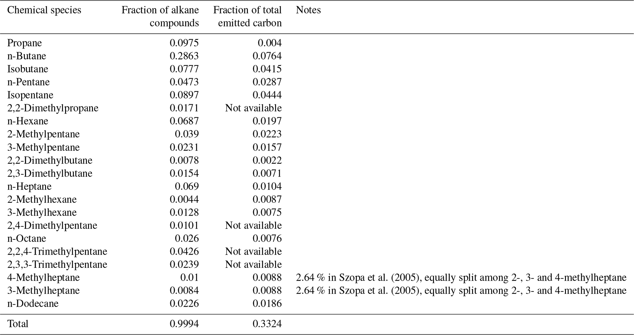
In both the ECLIPSE and the GFED4 databases, NMVOC emissions are lumped together. The CBM-Z module distinguishes 13 compounds/classes of NMVOCs; hence we have disaggregated NMVOC emissions into the CBM-Z compound/class using conversion factors from Szopa et al. (2005) and other sources. We have derived each compound/class emission by multiplying NMVOC emissions by the respective fraction of the total emitted carbon reported in Table 1. For lumped compounds (e.g. ACET, ketones, or PAR, paraffin carbon), the fraction of the total emitted carbon results from the sum of fractions of single compounds taken from Zaveri and Peters (1999) and Szopa et al. (2005) (Table 2).
Pozzer et al. (2007)Table 1Non-methane volatile organic compound speciation based on fractions of total emitted carbon as obtained from Table 1 in Szopa et al. (2005) or from other sources, when specified.
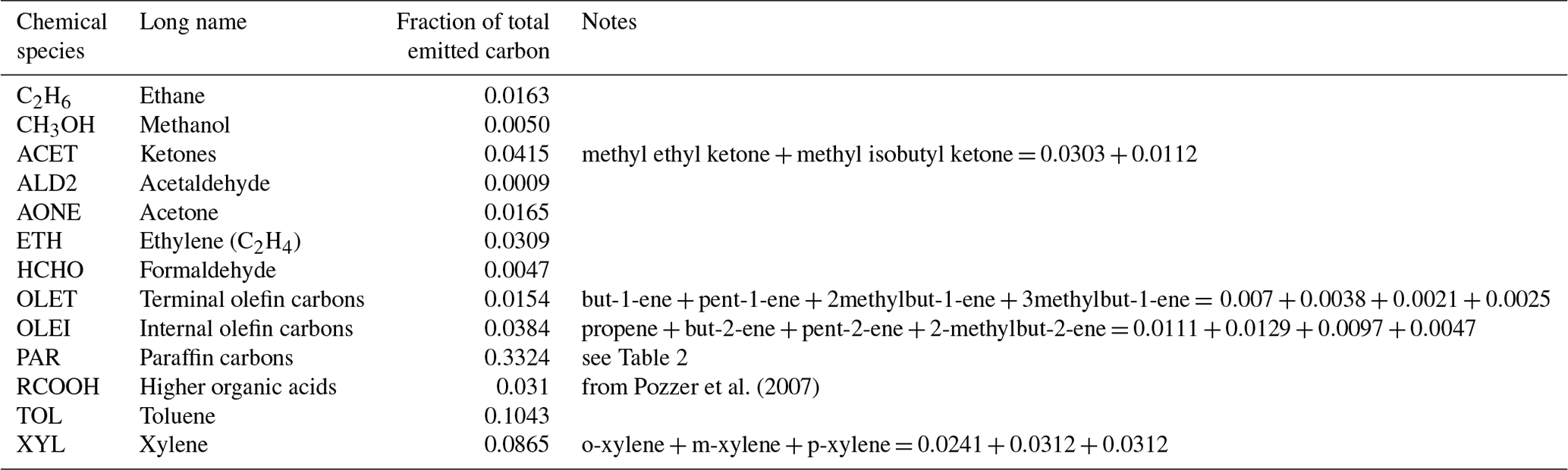
Table 2List of paraffin carbons as well as their related fraction of alkane compounds (Table 4 in Zaveri and Peters, 1999) and fraction of total emitted carbon (Table 1 in Szopa et al., 2005).
Chemical boundary conditions are taken from the 1999–2009 monthly climatology built on the global chemistry model Model for Ozone and Related chemical Tracers (MOZART) (Emmons et al., 2010). The species O2 and H2 are kept at fixed concentrations (Graedel et al., 1993).
The RegCM model handles the removal of chemical species via dry and wet deposition, with dry deposition representing the main sink for ozone. Dry deposition is parameterized for relevant species (including ozone) using the scheme of Zhang et al. (2003) which reproduces stomatal and non-stomatal uptake from plants and soil by applying three resistances in series: aerodynamic, quasi-laminar and bulk surface/canopy resistances.
More details on the CBM-Z module and the RegCM4chem model can be found in Zaveri and Peters (1999) and Shalaby et al. (2012).
2.2 Simulation and analysis design
We carry out atmosphere-only simulations with the RegCM4–CLM4.5 model, while we use the full model RegCM4chem–CLM4.5–MEGAN2.1 to run atmosphere–chemistry simulations. Both simulations include surface–atmosphere interactions, handled by the CLM4.5 land surface model. All simulations are run at a horizontal grid spacing of ∼25 km over the Med-CORDEX (Coordinated Regional Climate Downscaling Experiment in the Mediterranean region) domain (Ruti et al., 2016; https://cordex.org/domains/region-12-mediterranean/, last access: October 2023), forced with ERA-Interim reanalysis (Dee et al., 2011), which provides lateral and boundary conditions for both the atmosphere and the sea surface temperature every 6 h at a horizontal resolution of 0.75∘. Greenhouse gas concentrations follow the historical values from the Intergovernmental Panel on Climate Change (IPCC) Fifth Assessment Report (AR5) (van Vuuren et al., 2011). Stratospheric ozone is prescribed based on the dataset used for the Coupled Model Intercomparison Project (CMIP5) from the Stratosphere–Troposphere Processes and their Role in Climate (SPARC) project (Cionni et al., 2011), while aerosols are not accounted for. The total solar irradiance is taken from the CMIP5 solar forcing data (Lean et al., 1995).
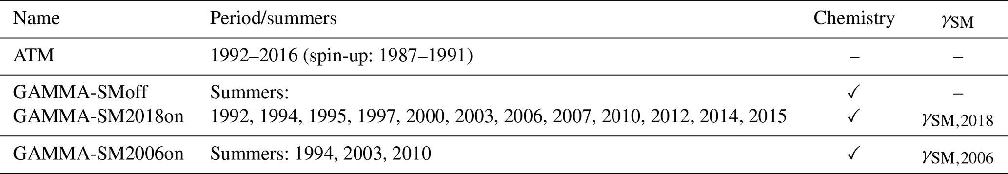
Firstly, we perform a control atmosphere-only simulation (named ATM), covering the 1987–2016 period (with a 5-year spin-up, 1987–1991). These simulations provide initial and lateral meteorological and surface conditions to drive the coupled atmosphere–chemistry simulations. This methodology ensures that at the first time step of each atmosphere–chemistry simulation atmospheric and soil conditions are realistic. The atmosphere–chemistry simulations are then carried out for 12 selected summers: 1992, 1994, 1995, 1997, 2000, 2003, 2006, 2007, 2010, 2012, 2014 and 2015, since summer is the season of maximum isoprene emissions and maximum production of near-surface ozone. These summers have been selected based on the 1970–2016 precipitation climatology derived from the E-OBSv20 dataset as those having dry or wet anomalies within the 1992–2016 period (Fig. S1 in the Supplement).
The summer atmosphere–chemistry simulations cover the periods May through August, with May assumed as spin-up to reach the equilibrium of chemical species (and thus not considered in the analysis). Each simulation is run twice: with (GAMMA-SM2018on) and without (GAMMA-SMoff) the new MEGAN soil moisture activity factor (γSM, 2018, Eq. 6). We then compare the GAMMA-SM2018on and GAMMA-SMoff simulations to evaluate the effect of soil moisture on isoprene emissions and near-surface ozone levels. We also select some extreme summers (i.e. 1994, 2003, 2010) to perform the same simulation using the old MEGAN soil moisture activity factor (γSM, 2006, Eq. 5, GAMMA-SM2006on) in order to compare the effects of the updates in the activity factor parameterization. To ensure there are no differences in the simulated climate across the atmosphere–chemistry simulations (GAMMA-SM2018on, GAMMA-SM2006on and GAMMA-SMoff), we do not account for the chemistry feedback on climate. Table 3 summarizes all performed simulations.
We focus our analysis on the summer atmosphere–chemistry simulations for the June–July–August (JJA) periods, when isoprene emissions and surface ozone levels are maximum over the Med-CORDEX domain. We compute the absolute differences in a variable X as , with the “∗on” referring to GAMMA-SM2018on or GAMMA-SM2006on simulations. Percentage changes in X are calculated relative to the GAMMA-SMoff simulation (i.e. ). When considering the old and new MEGAN soil moisture activity factors, we compare the GAMMA-SM2018on and GAMMA-SM2006on simulations against each other and also against the GAMMA-SMoff simulations.
We derive values of the soil moisture activity factor γSM by dividing isoprene emissions from the GAMMA-SM2018on (or the GAMMA-SM2006on) simulation by emissions from the reference simulation GAMMA-SMoff.
Except for the model evaluation of atmospheric fields, which considers the whole Med-CORDEX domain, our analysis encompasses part of the domain, whose coordinates are (28–58∘ N, 15∘ E–50∘ W); hereafter, we refer to this area as the Euro-Mediterranean region. To facilitate the model evaluation, the model output was remapped onto the observed data grid using a distance-weighted method, which conserves both the total field and its spatial structure (Torma et al., 2015).
3.1 Model evaluation
3.1.1 Atmospheric fields: temperature and precipitation
To evaluate means and extremes in temperature and precipitation, we use the E-OBS ensemble version 20e (E-OBSv20e), which provides daily land-only station-based gridded precipitation and surface air temperature (mean, minimum and maximum) over the 1950–2018 period at a resolution of 0.25∘ (Cornes et al., 2018). For cloud cover, we use the CLoud property dAtAset using SEVIRI (CLAAS, version 1) observation dataset produced by the European Organization for the Exploitation of Meteorological Satellites (EUMETSAT) within the Satellite Application Facility on Climate Monitoring (CM SAF) project, which is derived from the geostationary Meteosat Spinning Enhanced Visible and Infrared Imager (SEVIRI) measurements and provides global (between 65∘ S and 65∘ N), monthly mean, fractional cloud cover over the 1991–2015 period at a resolution of 0.05∘ (Stengel et al., 2014). Table S2 presents all observation-based datasets and their features, which we used for model evaluation in the present study.
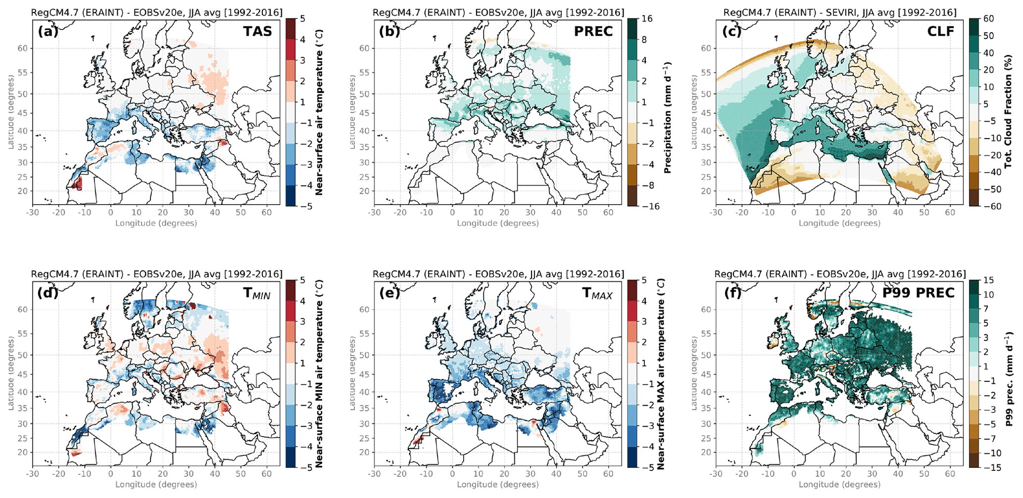
Figure 1Spatial distribution of summer (June–July–August, JJA) biases over the Med-CORDEX domain and over the 1992–2016 period in the (a) 2 m air temperature (units: ∘C), (b) precipitation rate (mm d−1), (c) total cloud fraction (unitless), (d–e) daily maximum and minimum 2 m air temperature (∘C), and (f) 99th percentile of the precipitation rate (P99 prec.; mm d−1). Biases correspond to differences between summer-averaged fields from the RegCM4–CLM4.5 model and (a, b, d–f) the E-OBSv20e dataset for temperature and precipitations and (c) the CLAAS dataset for total cloud fraction. For comparison, the model output was remapped onto the observation grid.
Figure 1 presents the spatial distribution of summer-averaged atmospheric biases for the 1992–2016 period. Compared to E-OBSv20e, the RegCM4–CLM4.5 model shows a prevailing cold bias between −3 and −2 ∘C across the Mediterranean Basin. Conversely, over south-western Russia, north-western Africa and Iraq, there is a warm bias of +1 to +2 ∘C (Fig. 1a). Overall, the bias absolute values are mostly in the range of 1 to 3 ∘C, which is in line with other regional climate simulations (Kotlarski et al., 2014; Vautard et al., 2021). For precipitation over land, RegCM4–CLM4.5 shows a prevailing wet bias across the domain in the range of +1 and +4 mm d−1, with larger biases in the mountainous regions (i.e. the Pyrenees, the Alps, the Carpathians) (Fig. 1b). Compared to the CLAAS dataset, the model tends to overestimate cloudiness (between 10 % and 40 % in terms of total cloud fraction) over the ocean and the Mediterranean Sea, as well as over northern Spain, southern France, northern Italy and northern Turkey (between 10 % and 20 %), while cloudiness is underestimated (between −5 % and −20 %) over the southern, eastern and northern parts of the domain (Fig. 1c). In terms of climate extremes, compared to E-OBSv20e, the summer bias in daily minimum temperatures shows both cold and warm bias, between −3 to +3 ∘C (Fig. 1d), while daily maximum temperatures show prevailing cold biases (between −5 and −1 ∘C) over nearly the entire domain (Fig. 1e). The model overestimates intense precipitation over most of the domain with a wet bias between +10 and +15 mm d−1 in the 99th percentile of daily precipitation (Fig. 1f). It is likely that the wet precipitation biases and the cold temperature ones are related, but overall the model performance for the present runs is in line with previous applications of the RegCM4 (e.g. Fantini et al., 2018).
3.1.2 Surface fields: latent heat flux and soil moisture
To evaluate surface latent heat flux as an indicator of evapotranspiration, we use the remote-sensed (RS) product from the FLUXCOM dataset (Jung et al., 2019), which provides monthly global gridded remote-sensed latent heat fluxes for 2001–2015 at a resolution of 0.5∘. The FLUXCOM dataset results from the upscaling of site-level energy flux observations from the global network of micro-meteorological flux measurement towers (FLUXNET eddy-covariance data) using a machine learning technique and combining in situ observations with remote sensing and land cover data (Jung et al., 2019). Compared to FLUXCOM over the Euro-Mediterranean region, RegCM4–CLM4.5 shows larger evapotranspiration during summer, over land-only grid cells (5–10 W m−2, Fig. 2a; +10 %–20 % percentage biases in Fig. S2), with the largest wet bias over north-eastern Spain (+20–40 W m−2; +40 %–80 %), while some areas located in the middle and southern part of the domain (Portugal, north-western Spain, western France, the middle of Italy, the Balkans, northern Africa and the Middle East) display a dry bias (between −5 and −20 W m−2, between −10 % and −20 %). From June to August, over land-only grid cells located in the southern part of the domain (below 50∘ N), the difference between the model and observation annual cycles is <5 W m−2 (Fig. 2b). The overestimation of latent heat flux is likely related to the overestimation of precipitation found in Sect. 3.1.1.
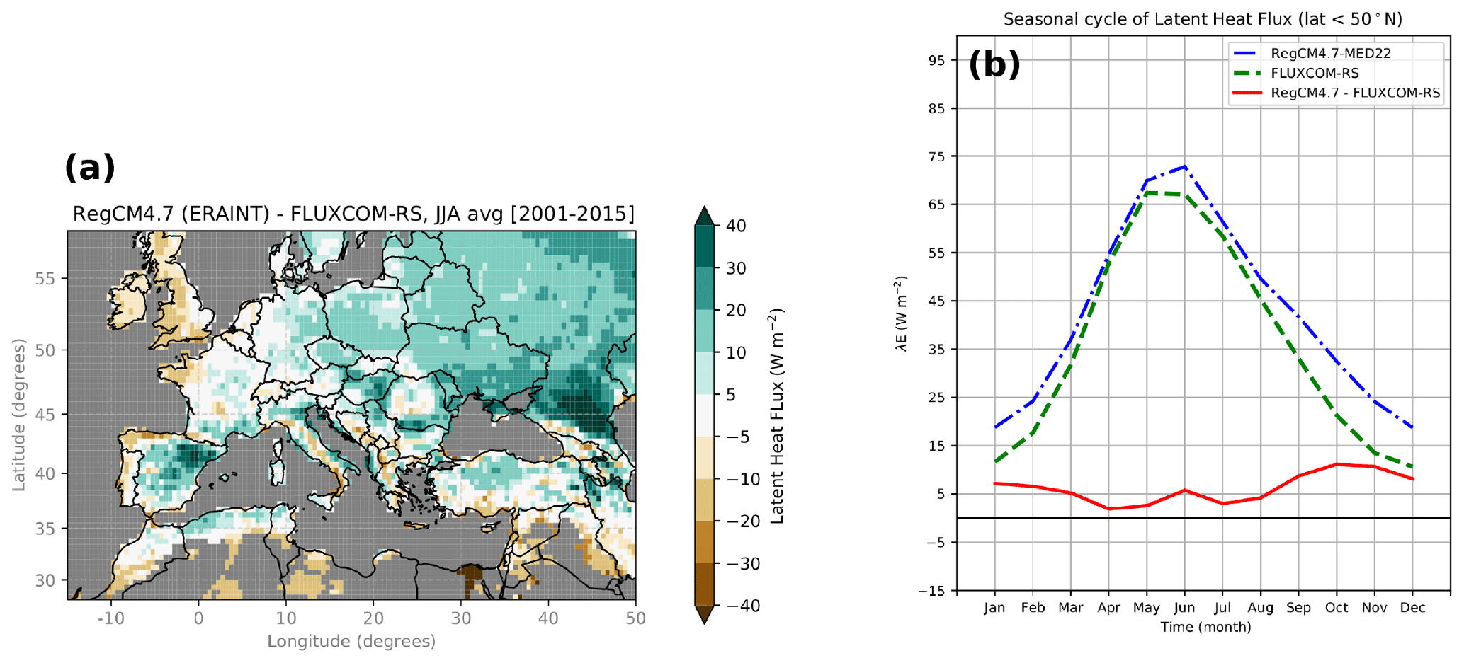
Figure 2Comparison of latent heat fluxes (units: W m−2) between the RegCM4–CLM4.5 model and the FLUXCOM dataset (remote-sensed product) over 2001–2015: (a) spatial distribution of summer bias and (b) annual cycles south of 50∘ N for the RegCM4–CLM4.5 model (blue line) and the FLUXCOM dataset (green line), as well as their difference (red line) as computed over the illustrated part of the model domain, hereafter referred to as the Euro-Mediterranean region (coordinates: (28–58∘ N, 15∘ E–50∘ W)). Biases correspond to differences between summer-averaged fields from the RegCM4–CLM4.5 model and the FLUXCOM dataset. For comparison, the model output was remapped onto the FLUXCOM grid.
For the evaluation of soil moisture, we use the global monthly gridded (0.25∘) surface soil moisture (SSM) data for 1978–2015 produced by the European Space Agency Climate Change Initiative (ESA-CCI, version 04.4) based on observations from both scatterometers and radiometers (Dorigo et al., 2017). The ESA-CCI dataset offers three products obtained from different sensor types: active (scatterometer only), passive (radiometer only) and combined (merged active and passive products), and here we use the combined product. Since the ESA-CCI dataset has many missing values over Europe before 2004, we focus our analysis on the 2005–2015 period. The ESA-CCI theoretical global mean sensing depth is ∼ 2 cm (Dorigo et al., 2017). Based on the soil thickness of the RegCM4 soil layers (Table S3), we compare ESA-CCI data with the first model soil layer (soil depth: 1.75 cm), which shows a similar pattern as the observed, with lower values in the eastern part of the domain (Fig. S3). Over the southern part of the Euro-Mediterranean region (south of 50∘ N), RegCM4–CLM4.5 follows the ESA-CCI volumetric soil moisture well and shows high correlation (r2=0.7), while the correlation is lower north of 50∘ N (r2=0.3), most probably due to the effect of snow at higher latitudes (Fig. 3a and b). South of 50∘, both RegCM4–CLM4.5 and ESA-CCI SSM show a bimodal distribution, which however peaks around lower values in RegCM4–CLM4.5 (below 0.1 m3 m−3 against 0.1 and 0.2 m3 m−3 for ESA-CCI SSM) and spans a larger range (up to 0.5 m3 m−3 vs. 0.4 m3 m−3 for ESA-CCI SSM) (Fig. 3c and d). Hence, compared to observations, the model more frequently reproduces very dry (below 0.1 m3 m−3) and very wet (above 0.4 m3 m−3) grid cells over the Euro-Mediterranean region.
Overall, compared to observations, RegCM4–CLM4.5 reproduces fields of evapotranspiration and soil moisture over the Euro-Mediterranean region quite well.
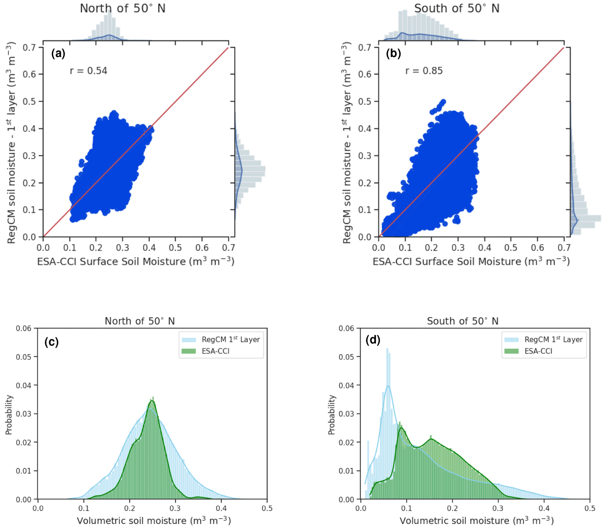
Figure 3Comparison of volumetric soil moisture (unit: m3 m−3) between the first soil layer in the RegCM4–CLM4.5 model and the ESA-CCIv4.04 dataset over the 2005–2015 period: (a, b) cloud plots and Pearson's r correlations between the RegCM4–CLM4.5 model (y axis) and the ESA-CCIv4.04 dataset (x axis) and (c, d) probability distributions of soil moisture from the RegCM4–CLM4.5 model (in blue) and the ESA-CCIv4.04 dataset (in green). Panels (a) and (c) refer to the area north of 50∘ N and (b) and (d) to the area south of 50∘ N in Fig. 2a. For comparison, the model output was remapped onto the ESA-CCI grid.
3.1.3 Chemical fields
Among the chemical species simulated by the RegCM4chem–CLM4.5–MEGAN2.1 model, we focus on isoprene, formaldehyde (HCHO) and near-surface ozone, and we evaluate the model output produced by the RegCM4chem–CLM4.5–MEGAN2.1 model in the GAMMA-SMoff simulation.
For isoprene, since there is no network over Europe routinely measuring isoprene concentrations in vegetated areas, we use in situ measurements of isoprene concentrations collected during two field campaigns that took place (1) in south-eastern France (site: La Verdière; latitude: 43.63∘ N, longitude: 5.93∘ E) during the summer of 2000 (from 21 June to 6 July) in the framework of the ESCOMPTE field campaign (Cros et al., 2004) when isoprene concentrations had been measured every 30 min using a fast isoprene sensor and (2) in Cyprus (site: Ineia; latitude: 34.96∘ N, longitude: 32.39∘ E) during the summer of 2014 (from 7 July to 3 August; data collected every 45 min) using the technique of gas chromatography–mass spectrometry (GC–MS) (Derstroff et al., 2017). Figure 4 shows the comparison between summer isoprene concentrations as observed at the two filed sites (La Verdière, France; and Ineia, Cyprus) and as simulated by the RegCM4chem–CLM4.5-MEGAN2.1 model (GAMMA-SMoff simulation) at the grid cell nearest to the observation spot. In general, the model underestimates isoprene concentrations at both locations (La Verdiére and Ineia), and sometimes it reproduces a delayed peak in isoprene concentrations compared to observations. Differences between observations and the model output could result from multiple factors: (i) the cold and wet model bias that limits isoprene emissions; (ii) differences between vegetation types in the field and in the model grid cell; and (iii) different scales with a model grid cell spanning a surface of hundreds of square kilometres, while station measurements have a footprint of a hundreds of metres.
In addition, to evaluate isoprene emissions, we use satellite retrievals of formaldehyde, an intermediate by-product of the oxidation of hydrocarbons such as methane and BVOCs. Although the oxidation of methane represents the dominant source of formaldehyde (60 %) followed by the oxidation of BVOCs (30 %) (Stavrakou et al., 2015), methane contributes to the background abundance of formaldehyde in the troposphere (Fowler et al., 2009), while isoprene drives major variations in formaldehyde concentrations in the boundary layer, with contributions of up to 85 % during the growing season (Franco et al., 2016) at a spatial scale of ca. 10–100 km (Palmer et al., 2003). Thus, retrievals of HCHO provides a good surrogate to evaluate the model performance in reproducing isoprene emissions.
To evaluate the formaldehyde burden, we use retrievals of HCHO column concentrations from the Ozone Monitoring Instrument (OMI), a nadir-viewing UV–Vis solar backscatter instrument, travelling aboard the Aura satellite (Stavrakou et al., 2018). These are gridded level-3 monthly mean data produced in the framework of the EU FP7 Quality Assurance for Essential Climate Variables project, version QA4ECV (De Smedt et al., 2015), covering the 2005–2016 period at a resolution of 0.25∘. Focusing on land-only grid cells in the Euro-Mediterranean region, for the simulated summers within the OMI observing period (2005–2016), RegCM4chem–CLM4.5–MEGAN2.1 shows similar distributions of summer-averaged HCHO column concentrations as those observed. However, the model has lower median values and a smaller variability in maximal outliers (Fig. 5). This result is consistent with the model underestimating isoprene concentrations compared to in situ measurements. The summer of 2010, when a heat wave hit Russia with associated wildfires (Barriopedro et al., 2011), stands out as the summer when the model does not capture the largest median value of HCHO columns, although the model shows larger variability in outliers. These differences may be related to the cold and wet biases identified for the RegCM4–CLM4.5 model (Sect. 3.1.1) since warm atmospheric conditions favour BVOC production and emissions and, lastly, influence HCHO columns. Negative values in the OMI dataset indicate high noise in the data over areas with low-HCHO columns, mainly located over northern Africa in the chosen domain.
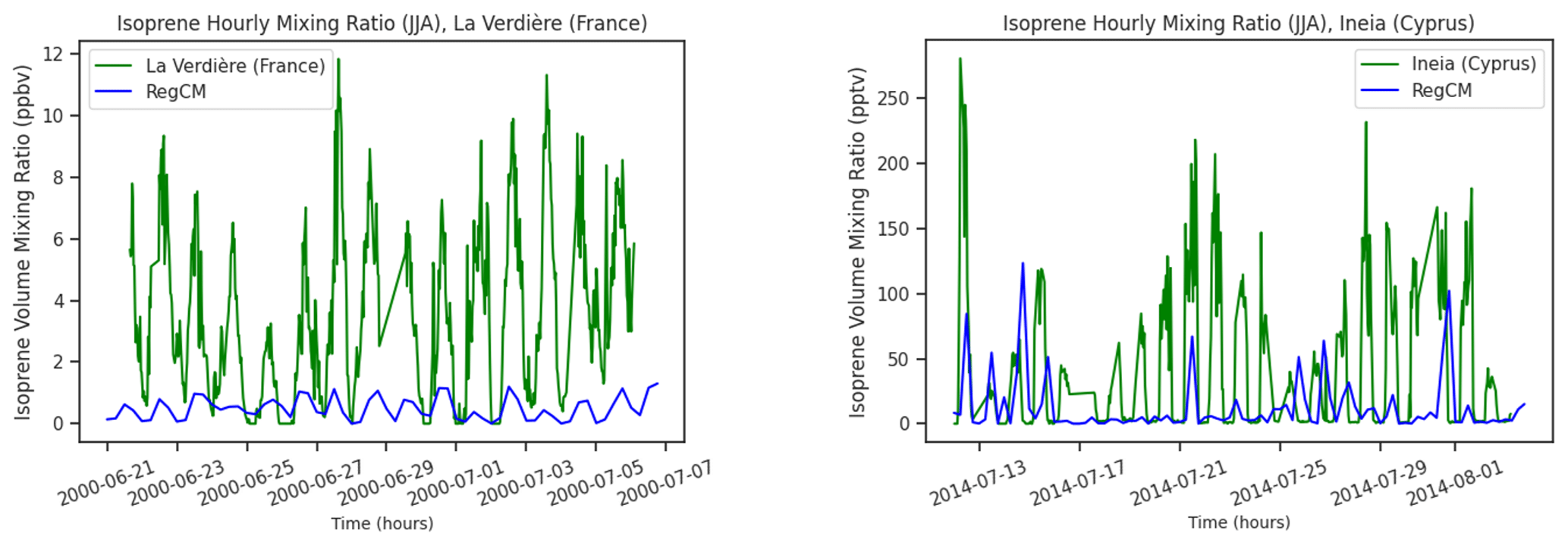
Figure 4Comparison of the time series of isoprene concentrations collected at La Verdière (latitude: 43.63∘ N, longitude: 5.93∘ E; France, summer 2000; units: ppbv) and at Ineia (latitude: 34.96∘ N; longitude: 32.39∘ E; Cyprus, summer 2014; units: pptv). The solid green line shows observations, while the solid blue line shows the model output extracted from the grid cell nearest to the observation spot from the GAMMA-SMoff simulation performed with the RegCM4chem–CLM4.5–MEGAN2.1 model.
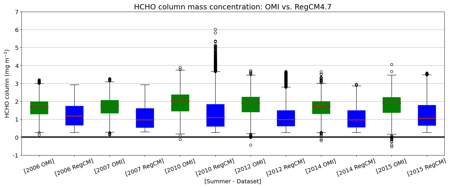
Figure 5Box-and-whisker plots showing the distribution of the summer-averaged mass column concentrations of formaldehyde (HCHO) (units: mg m−2) as observed by the Ozone Monitoring Instrument (OMI; version QA4ECV; green boxes) and as reproduced by the RegCM4chem–CLM4.5–MEGAN2.1 model (blue boxes) over land-only grid cells in the Euro-Mediterranean region (see Fig. 2a) and across simulated summers over the OMI observational period, 2005–2016. The boxes display the interquartile range (Q25, Q75), with the orange line showing the median value; the whiskers cover from to ; and the empty black circles represent outliers. Negative values in the OMI dataset reflect the high noise in the data detected over scenes with low-HCHO columns. For comparison, the model output has been remapped onto the OMI grid.
To evaluate near-surface ozone, we use air quality measurements collected by the European Environment Agency (EEA) that provide observations over different European countries (https://www.eea.europa.eu/data-and-maps/data/aqereporting-9, last access: June 2022). In Fig. 6 the summary of the comparison is presented, focusing on the summer of 2015 and using daily means. Although RegCM4chem–CLM4.5–MEGAN2.1 underestimates ozone concentrations compared to the EEA dataset over the three selected countries (i.e. Italy, Spain and France) and the Airbase observations span until very low values (close to 0), observed and modelled ozone concentrations differ with less than 50 µg m−3 over Italy and less than 25 µg m−3 over Spain and France. Additional comparisons against the reanalyses from the Copernicus Atmosphere Monitoring Service (CAMS; Marécal et al., 2015) for the 2003–2007 period shows that the model performs well over land (differences lower than 10 ppbv), while it underestimates near-surface ozone over the Mediterranean Basin, with differences spanning between 10 and 20 ppbv and with some summers and some grid cells showing larger differences, up to 30 ppbv (Fig. S4).
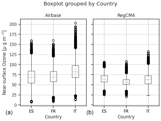
Figure 6Box-and-whisker plots showing the distribution of summer daily mass concentrations of near-surface ozone levels (O3) (units: µg m−3) as observed by the Airbase monitoring network (a) and as reproduced by the RegCM4chem–CLM4.5–MEGAN2.1 model (b) over the summer of 2015 over Spain (ES), France (FR) and Italy (IT). The boxes display the interquartile range (Q25, Q75), with the orange line showing the median value; the whiskers cover from to ; and the empty black circles represent outliers. For comparison, the model output has been taken at the grid cell closest to each Airbase station.
3.2 Effect of water stress on isoprene emissions
In MEGAN2.1, the activity factor γSM, 2018 spans between 0 and 1, and, based on the intensity of water stress, it reduces isoprene emissions (Eq. 6). Figure 7 shows the spatial distribution of the unitless summer-averaged soil moisture activity factor γSM, 2018 across the simulated summers and across areas where vegetation can grow (desert areas are in grey), while Fig. 8 shows the spatial distribution of summer percentage changes in isoprene emissions (absolute changes in Fig. S5). Low values of the soil moisture activity factor () indicate a sustained water stress and are located over dry climates such as over northern Africa and the Middle East (Fig. 7). In these areas isoprene emissions decrease by more than 80 % when the effect of water stress is accounted for in numerical simulations (Fig. 8). Mid and high values () correspond to a mild and low water stress and are located over areas that experienced a dry anomaly based on the 1970–2016 precipitation climatology (Fig. S1 vs. Fig. 7). Over these areas, isoprene emissions decrease between −5 % and −60 % (Fig. 8) (absolute changes between −0.50 and −12.0 mg m−2 d−1, Fig. S5).
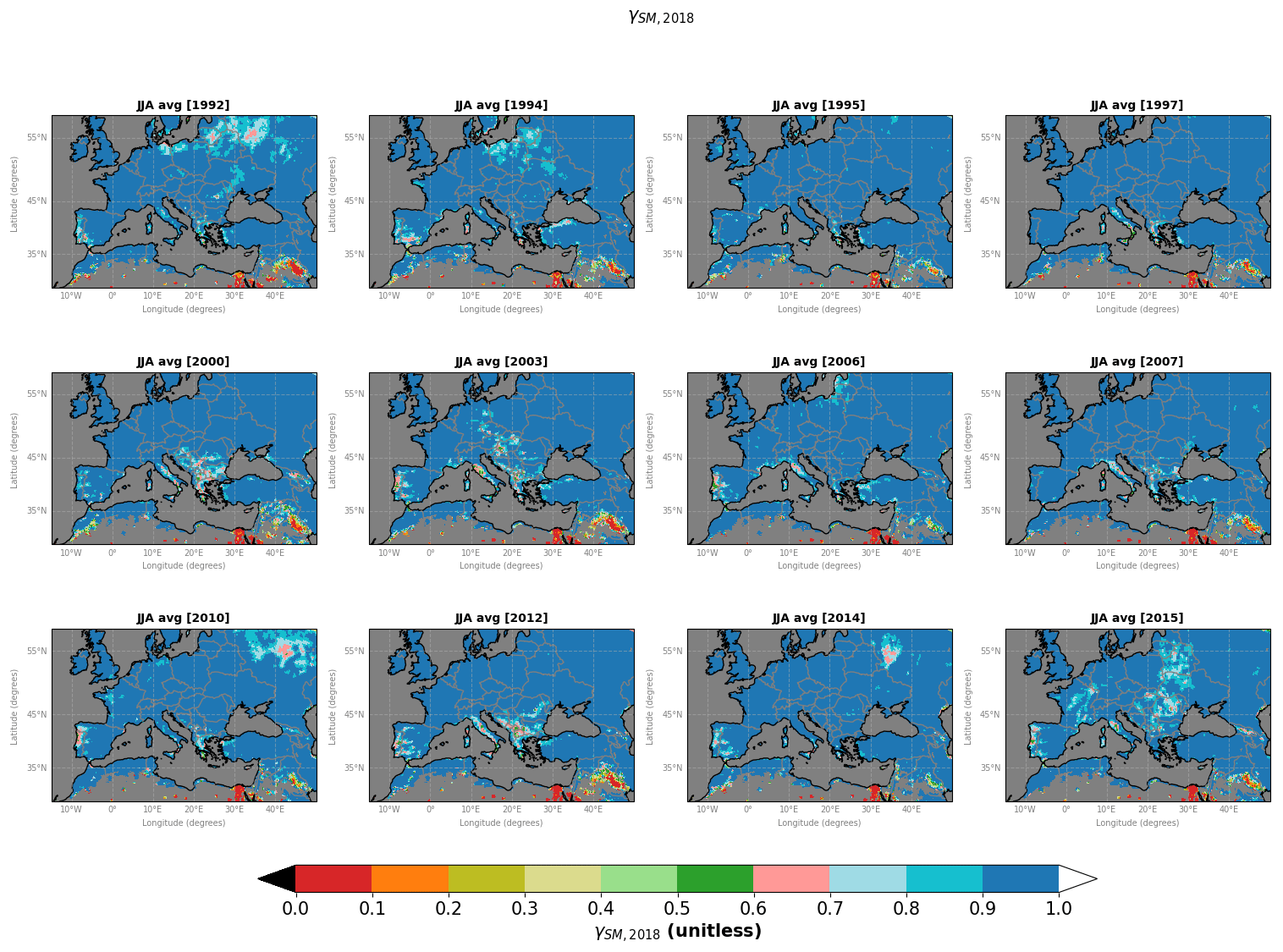
Figure 7Spatial distribution of the summer-averaged soil moisture activity factor γSM,2018 (unitless) as simulated by the RegCM4chem–CLM4.5–MEGAN2.1 model over the Euro-Mediterranean region and across selected summers over 1992–2016. The γSM,2018 factor ranges between 0 (severe water stress) to 1 (no water stress) and was derived by dividing isoprene emissions from the GAMMA-SM2018on simulation by emissions from the reference simulation GAMMA-SMoff. The grey areas correspond to grid cells where isoprene emissions are not defined.
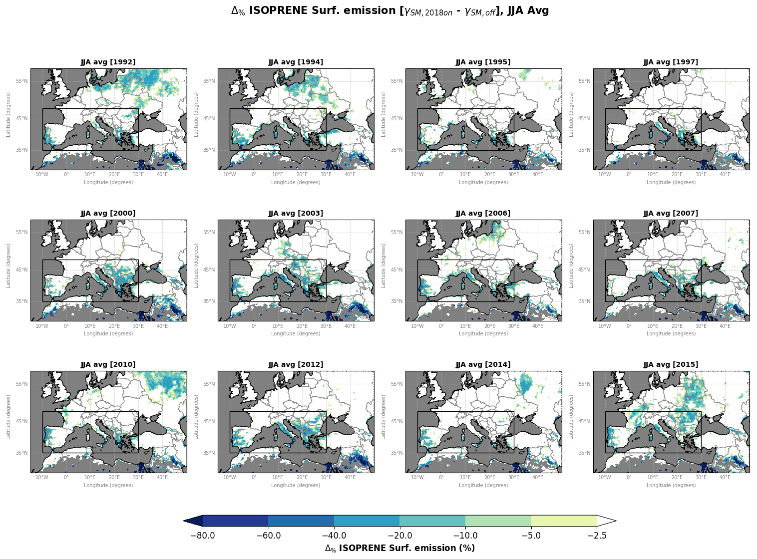
Figure 8Spatial distribution of the summer-averaged percentage changes in isoprene emissions (units: %) as simulated by the RegCM4chem–CLM4.5–MEGAN2.1 model over the Euro-Mediterranean region and across selected summers over 1992–2016. To compute percentage changes, the difference between JJA averages from the GAMMA-SM2018on (γSM, 2018) and the GAMMA-SMoff simulations was divided by the reference simulation GAMMA-SMoff. The black boxes highlight the area of southern Europe selected for further analysis.
Simulated decreases in isoprene emissions are similar to those simulated using a global climate model over Europe in the year 2010 by Jiang et al. (2018), who found a decrease in isoprene emissions over Europe with a maximum in August and spanning between 0 and −2 mg m−2 h−1. In the summer of 2010, the RegCM4chem–CLM4.5–MEGAN2.1 model also reproduced the largest decrease in isoprene emissions, with a maximum reduction of −76 mg m−2 d−1 simulated in July and located over south-western Russia (latitude: 60.24∘ N; longitude: 39.88∘ E) where drought and an extreme heat wave occurred (Barriopedro et al., 2011). Such a substantial reduction in isoprene emissions corresponds to −3 mg m−2 h−1 (not shown). Compared to another high-isoprene-emission region such as the south-eastern US, the Euro-Mediterranean region shows similar reductions in summer isoprene emissions, between −10 % and −20 %, to those simulated by Klovenski et al. (2022).
Table 4 presents absolute and percentage changes in isoprene emissions and near-surface ozone mixing ratios averaged over the Euro-Mediterranean region. Over this region and across the simulated summers, isoprene emissions decrease by 6 % on average (−0.3 mg m−2 d−1), mirroring the spatial and temporal patterns of the 1970–2016 precipitation anomaly (see Figs. S1 and 8). In particular, a “wet” summer, such as the summer that occurred in 1997, shows the smallest reduction in isoprene emissions over the Euro-Mediterranean region (−0.16 mg m−2 d−1, −5.09 %), while a “dry” summer, such as the summer of 2012, displays the largest absolute reduction (−0.48 mg m−2 d−1, −8.11 %). Among all simulated summers, the summer of 2000 has the largest percentage reduction (−0.47 mg m−2 d−1, −8.41 %) since a large dry anomaly occurred in the Balkans, a region characterized by elevated isoprene emissions. The largest decreases in isoprene emissions occur in the summers of 2003 and 2012 (Table 4), when the observation-based summer temperatures are nearly 4–5 standard deviations above (warmer than) the 1970–1990 climatology (Fig. S6). These results suggest that isoprene emissions would be strongly reduced when heat waves and droughts co-occur.
Table 4The absolute and percentage changes in summer isoprene emissions and near-surface ozone mixing ratios averaged over the Euro-Mediterranean region (see Fig. 2a) and computed across the simulated summers. Changes correspond to the difference between summer means from the GAMMA-SM2018on (or GAMMA-SM2006on) and the GAMMA-SMoff simulations. The percentage changes were obtained by dividing the absolute changes by the reference simulation, GAMMA-SMoff.

Decreases in isoprene emissions drive decreases in formaldehyde concentrations that range between −5 % and −20 % (Fig. S7). As shown in Sect. 3.1.3, the RegCM4chem–CLM4.5–MEGAN2.1 model underestimates HCHO columns in its standard configuration (Fig. 5). The activation of a soil moisture activity factor in MEGAN (i.e. γSM, 2018 or γSM, 2006) decreases isoprene emissions due to the effect of water stress and, as a consequence, decreases HCHO concentrations and does not improve the comparison with OMI HCHO observations. On the contrary, the models used by P. Wang et al. (2021), Klovenski et al. (2022) and Wang et al. (2022) overestimate HCHO columns in their standard configurations; hence the indirect effect of the MEGAN soil moisture activity factor on HCHO concentrations improves the comparison between modelled and observed formaldehyde.
3.3 The link between anomalies in soil moisture and plant productivity and changes in isoprene emissions
When the MEGAN soil moisture activity factor γSM, 2018 is activated, dry anomalies limit isoprene emissions. Figure 9 shows the spatial distribution of summer anomalies in the total volumetric soil moisture used by vegetation and gross primary productivity (GPP; hereafter also referred to as plant productivity) as simulated by the RegCM4–CLM4.5 1 model for the simulated summers. Spatially, the anomalies in plant productivity overlap and correspond in signs with the anomalies in soil moisture that, in turn, follow the anomalies in precipitation (Figs. 9 and S1). Where dry anomalies occur, isoprene emissions decrease when the MEGAN soil moisture activity factor is activated (Fig. 9 vs. Fig. 8).
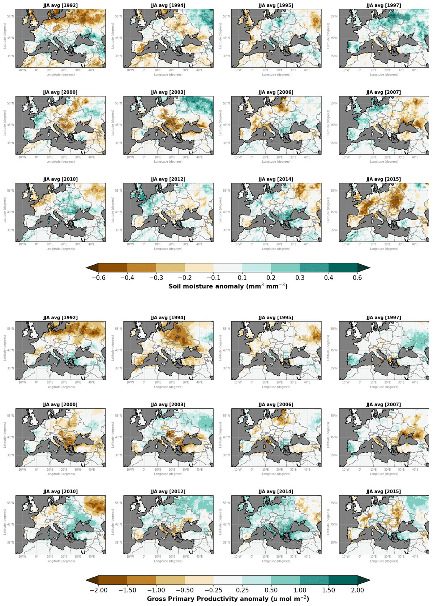
Figure 9Spatial distribution of the summer anomalies in soil moisture used by vegetation (units: mm3 mm−3) and gross primary productivity (GPP; units: µmol m−2) as simulated by the RegCM4–CLM4.5 model over the Euro-Mediterranean region and across selected summers over 1992–2016.
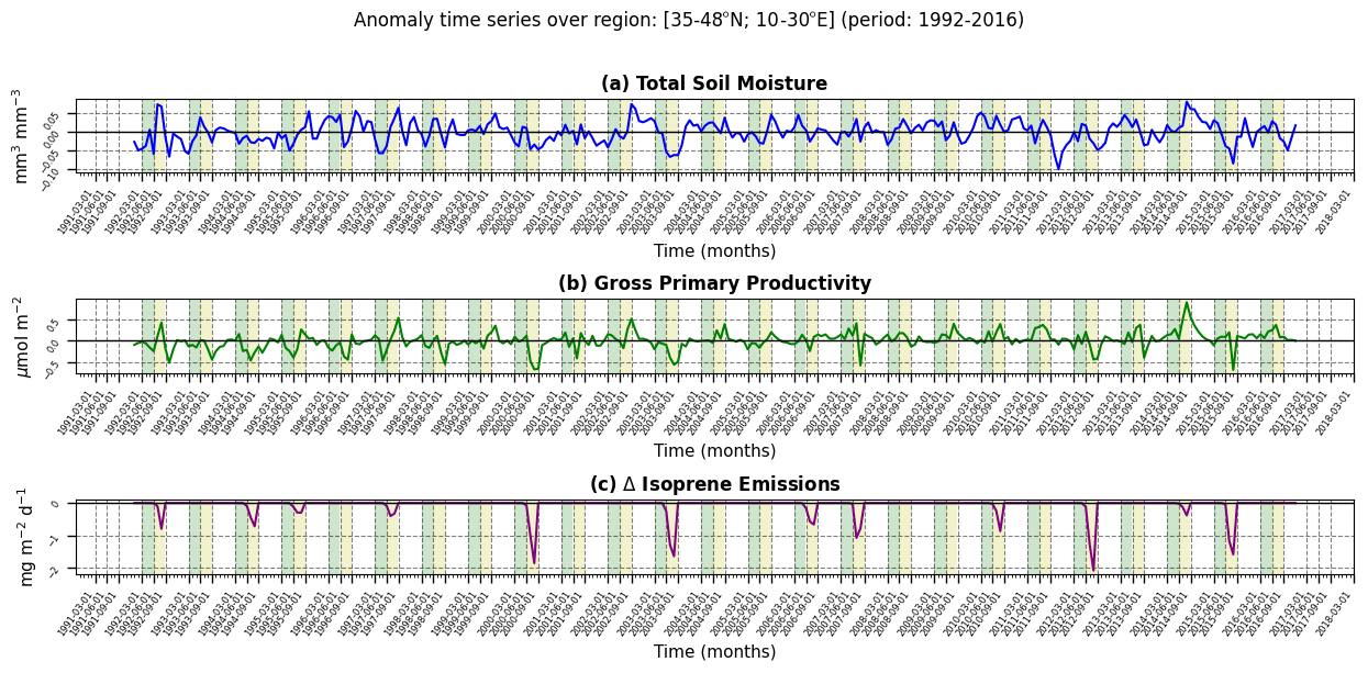
Figure 10Time series of the monthly anomalies in the (a) total soil moisture used by vegetation (units: mm3 mm−3; blue line), (b) gross primary productivity (GPP; units: µmol m−2; green line) and (c) absolute change in the monthly means of isoprene emissions (units: mg m−2 d−1; purple line). Anomalies and means were computed over the central part of the domain (black box in Fig. 8; coordinates: (35–48∘ N, 10∘ E–30∘ W)). Absolute changes in isoprene emissions correspond to the difference between monthly averages from the GAMMA-SM2018on and the reference simulation, GAMMA-SMoff, across selected summers over 1992–2016. The green (yellow) stripes highlight the spring, March–April–May, (summer, June–July–August) season.
Focusing on southern Europe (black box in Fig. 9), Fig. 10 shows the time series of the monthly anomalies in the total soil moisture used by vegetation and photosynthesis, as well as absolute monthly changes in isoprene emissions. All values are averaged over the (35–48∘ N; 10∘ E–30∘ W) area. Negative anomalies in soil moisture and plant productivity are in phase with the decrease in isoprene emissions. The summers of 2000, 2003, 2012 and 2015 display the most intense dry anomalies in soil moisture, leading to negative anomalies in plant productivity and, subsequently, to important decreases in isoprene emissions (−2 mg m−2 d−1). Among these summers, the summer of 2012 shows the largest decrease in isoprene emissions, most likely due to the combined effect of the driest anomaly in soil moisture between the years 2011 and 2012, followed by a short wet anomaly during spring and an intense dry anomaly during summer. A lagged effect probably due to a dry autumn and winter also plays an important role during the summer of 2010, when isoprene emissions decrease substantially, although both soil moisture and plant productivity show positive summer anomalies. Using meteorological observations and simulations, Vautard et al. (2007) found that hot summers over Europe are correlated with winter to early spring precipitation deficits in southern Europe.
3.4 The effects of changes in isoprene emissions on near-surface ozone levels
Under the effect of water stress, the RegCM4chem–CLM4.5–MEGAN2.1 model simulates a reduction in isoprene emissions that influences levels of near-surface ozone. Figure 11 shows the spatial distribution of summer percentage changes in the near-surface ozone mixing ratio when the water stress factor is activated. Decreases in isoprene emissions reduce near-surface ozone levels by less than 2 % (Fig. 11; absolute reduction <2 ppbv, Fig. S8). Over Europe, Jiang et al. (2018) obtained a similar decrease in near-surface ozone with a 6-month atmosphere–chemistry–vegetation simulation with the earth system model CAM–chem-CLM4.5–MEGAN2.1 at a coarser resolution (1.9∘ × 2.5∘ spatial res.). Similarly, Guion et al. (2023) simulated a decrease in near-surface ozone of −5 % over the Po Valley using the chemistry-transport model CHIMERE. Such a small decrease in near-surface ozone levels may be due to a dominant VOC-limited regime, where ozone decreases by lowering VOC emissions, reproduced by the RegCM4chem–CLM4.5–MEGAN2.1 model over the whole domain, as shown in Fig. S9 by computing the ratio between formaldehyde and nitrogen dioxide (NO2) based on Duncan et al. (2010).
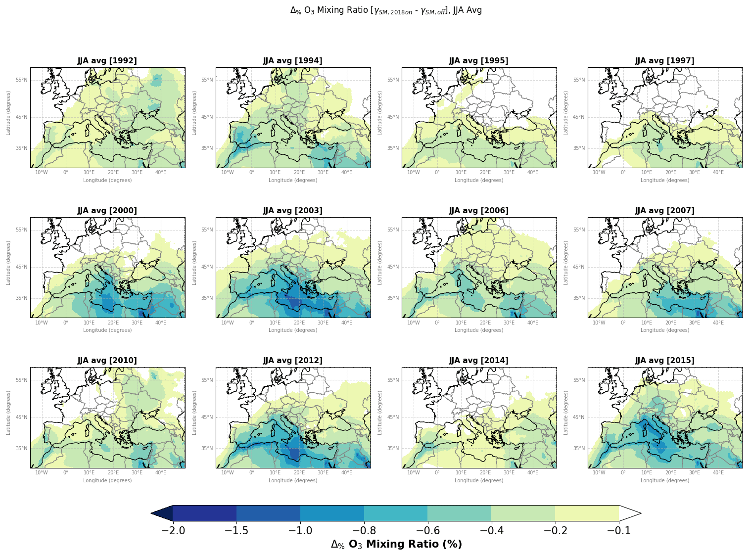
Figure 11Spatial distribution of summer-averaged percentage changes in the ozone (O3) mixing ratio at 1000 hPa (units: %) as simulated by the RegCM4chem–CLM4.5–MEGAN2.1 model over the Euro-Mediterranean region and across selected summers over 1992–2016. To compute percentage changes, the difference between summer averages from the GAMMA-SM2018on and the GAMMA-SMoff simulations was divided by the reference simulation, GAMMA-SMoff.
Spatially, the largest reductions in near-surface ozone levels are observed over the southern and eastern part of the Mediterranean Basin (Fig. 11). Multiple modelling studies have identified a pronounced land–sea gradient in near-surface ozone levels, with higher concentrations over the Mediterranean Basin and the Middle East and lower concentrations over continental Europe and northern Africa (Jaidan et al., 2018, with references therein). In particular, in the eastern Mediterranean Basin, ozone production is favoured by the transport of ozone precursors, mainly from the European continent, and by stagnant meteorological conditions dominating during summer (Gerasopoulos et al., 2005). This pattern of near-surface ozone levels over the Mediterranean Basin most likely influences the spatial distribution of changes (Fig. 11).
As for isoprene emissions, the wet summer of 1997 shows the smallest reduction in near-surface ozone levels (−0.06 ppbv, −0.14 %). Instead, the largest reduction in near-surface ozone, of about −0.17 ppbv (−0.42 %), is found in the summer of 2003, when a heat wave hit Europe (Table 4) due to the temperature effect on ozone chemistry. Indeed, the summer of 2003 shows the largest and widest warm anomaly in surface air temperatures (Fig. S6).
3.5 Comparison of the two soil moisture activity factors and their effects on isoprene and near-surface ozone
The choice of the soil moisture activity factor in MEGAN2.1 influences the pattern and the magnitude of changes in isoprene emissions and near-surface ozone levels, as we tested for the summers of 1994, 2003 and 2010. Focusing on the summer of 2003 when Europe was struck by a series of heat waves, Fig. 12 displays the spatial distribution of the old and new MEGAN soil moisture activity factors, γSM, 2006 and γSM, 2018, respectively. The old MEGAN soil moisture activity factor γSM, 2006 shows low and mid values between 0 and 0.6 over the Euro-Mediterranean region, with values lower than 0.4 over northern Africa and between 0.4 and 0.6 across Europe. In contrast, the new MEGAN soil moisture activity factor γSM, 2018 varies across the whole scale of values (from 0 to 1) and shows some areas where there is no water stress (in white) and localized areas with middle values (between 0.3 and 0.7). For example, over Italy and the Balkans, which show the largest soil moisture anomalies during the summer of 2003 (see Fig. 9), γSM, 2006 has a homogeneous pattern with values between 0.4 and 0.5, while γSM, 2006 has values between 0.5 and 0.7 over small areas.
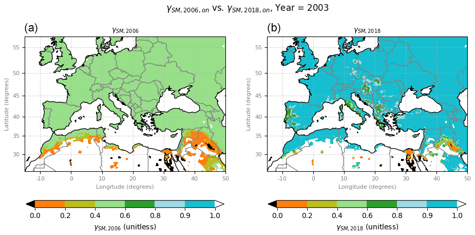
Figure 12Spatial distribution of the summer-averaged soil moisture activity factors γSM,2006 (a) and γSM,2018 (b) (unitless) over the Euro-Mediterranean region and for the summer of 2003.
The pattern and magnitude of the soil moisture activity factor influence the spatial distribution of changes in isoprene emissions (Fig. 13). Using the old soil moisture activity factor γSM, 2006, isoprene emissions decrease by more than 25 % over the Euro-Mediterranean region, with absolute decreases spanning from −0.5 up to −12 mg m−2 d−1. Once averaged over the Euro-Mediterranean region, decreases in isoprene emissions are around −3 mg m−2 d−1 (−57 %, Table 4). Over Australia and China, Emmerson et al. (2019) and Y. Wang et al. (2021) found similar decreases in isoprene emissions using the Guenther et al. (2006) parameterization (i.e. γSM, 2006). Conversely, when applying the new soil moisture activity factor γSM, 2018, isoprene emissions decrease by much lower magnitudes, with percentage changes between −5 and −25 % and larger reductions in the Middle East ( %). Over most of the Euro-Mediterranean region, decreases in isoprene emissions are smaller than 2.5 % ( mg m−2 d−1).
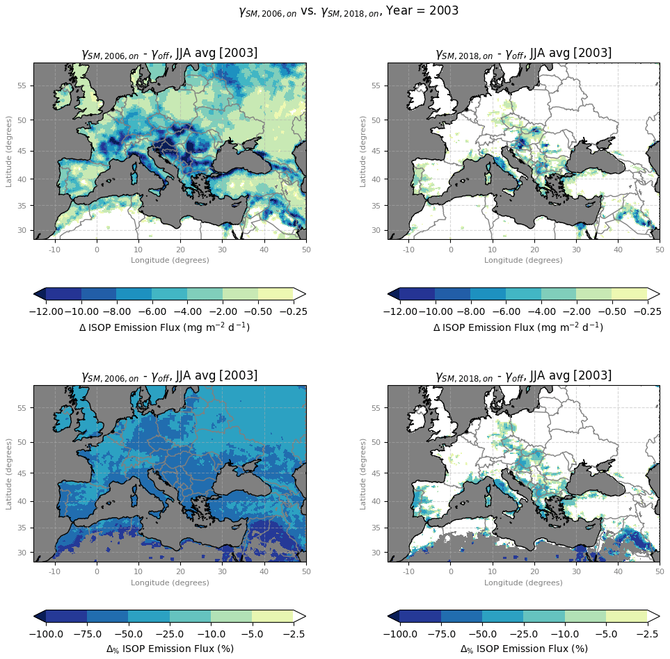
Figure 13Spatial distribution of the summer-averaged absolute (units: mg m−2 d−1) and percentage (%) changes in isoprene emissions computed over the Euro-Mediterranean region and for the summer of 2003 using the γSM,2006 and γSM,2018 soil moisture activity factors. Changes correspond to differences between summer averages of the model output from the GAMMA-SMon and the GAMMA-SMoff simulations using the old (γSM, 2006, GAMMA-SM2006on) or the new (γSM, 2018, GAMMA-SM2018on) soil moisture activity factor.
Concerning the effects on near-surface ozone, when applying the old soil moisture activity factor, near-surface ozone levels decrease homogeneously by ∼10 % (between −1.2 and 7.5 ppbv) over the Euro-Mediterranean region, with reductions between −2.5 % and −5 % over Europe and between −5 % and −10 % over the Mediterranean Basin (Fig. 14). Once averaged over the Euro-Mediterranean region, decreases in the near-surface ozone mixing ratio are around −3 ppbv (−4 %, Table 4). Similarly, using the Guenther et al. (2006) parameterization (i.e. γSM, 2006) over China, P. Wang et al. (2021) found that decreases in isoprene emissions reduce near-surface ozone with up to −8 % in drought-hit regions and during dry years. Conversely, when using the new soil moisture activity factor, near-surface ozone levels are not reduced by more than −1.5 %.
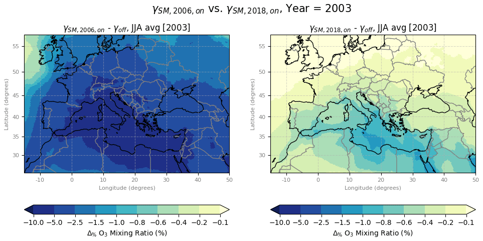
Figure 14As Fig. 13 – spatial distribution of the summer-averaged percentage changes (units: %) in the ozone mixing ratio at 1000 hPa for the summer of 2003.
The water stress effects on isoprene emissions and near-surface ozone mixing ratios were investigated for selected dry and wet summers in the Euro-Mediterranean region, using a regional vegetation–chemistry–climate model. This model includes the BVOC emission model MEGAN which provides two parameterizations limiting isoprene emissions under water stress. By performing sensitivity simulations, we assessed the decrease in isoprene emissions due to water stress and its impact on near-surface ozone mixing ratios. Moreover, we compared the two parameterizations available in MEGAN: the Guenther et al. (2006) and the Jiang et al. (2018) parameterizations.
Our results show that, over the Euro-Mediterranean region, water stress reduces isoprene emissions on average by 6 %, with larger decreases of up to 40 %–60 % over sensitive areas (e.g. the Balkans) and during very dry summers (e.g. 2003, 2015). Sustained decreases in isoprene emissions not only co-occur with negative anomalies in precipitation, soil moisture and plant productivity, but also are influenced by the lagged effect of prolonged or repeated dry anomalies, as observed for the summers of 2010 and 2012. This result confirms that it is critical to correctly initialize soil moisture for atmospheric–chemistry–vegetation numerical experiments. Regarding the indirect impact of water stress on near-surface ozone, our results suggest that over the Euro-Mediterranean region near-surface ozone levels have a limited sensitivity to decreases in isoprene emissions, with reductions in near-surface ozone by a few percent, most likely due to a dominant VOC-limited regime over the region, in agreement with Jiang et al. (2018). When comparing the two MEGAN parameterizations of water stress impact on isoprene emissions, we found substantial differences in the reduction of both isoprene emissions and near-surface ozone mixing ratios. Compared to the Guenther et al. (2006) parameterization, the Jiang et al. (2018) parameterization leads to more localized and 25 %–50 % smaller decreases in isoprene emissions and 3 %–8 % smaller reductions in near-surface ozone mixing ratios.
To summarize, our results (1) confirm the importance of soil moisture initialization when performing atmospheric–chemistry–vegetation numerical experiments, (2) show that the choice of the MEGAN parameterization to account for water stress impacts on isoprene emissions produces different reductions in ozone levels and (3) suggest that the indirect effect of water stress on ozone levels via changes in isoprene emissions is limited over the Euro-Mediterranean region. Our results are partly influenced by the prevailing cold temperature and wet precipitation biases identified for the RegCM4–CLM4.5 model. Warm atmospheric conditions favour both isoprene emissions and the production of near-surface ozone; hence a model characterized by a cold–wet bias most likely has a negative bias in reproducing isoprene emissions and near-surface ozone levels. Nevertheless, our results compare well with similar studies (Jiang et al., 2018; Emmerson et al., 2019; Y. Wang et al., 2021; Klovenski et al., 2022). While we observed an opposite sensitivity of isoprene emissions to the two parameterizations compared to the study by Guion et al. (2023), who obtained a larger decrease in isoprene emissions (−39 %) when using an adapted formulation of Jiang et al. (2018) and a smaller decrease (−12 %) when using the Guenther et al. (2006) parameterization. This result confirms the conclusions of Klovenski et al. (2022), who highlighted the need for tuning the MEGAN soil moisture activity factor and its parameters, based on the modelling set-up, which influences the soil moisture activity factor. In a future study, we aim to explore the ozone climate penalty over the Euro-Mediterranean region under both present-day and future climates and to assess the impact of both the direct effect of high temperatures and the indirect effect of water stress on isoprene emissions on ozone concentration.
To isolate the water stress impact on isoprene emissions and near-surface ozone, we chose to not account for aerosols (natural and anthropogenic) and the chemistry feedback on climate. A fully coupled vegetation–chemistry–climate model may produce different results, with aerosols (time varying or constant) influencing surface solar radiation, surface air temperature, cloud cover, evapotranspiration over land and lastly relative humidity (Boé et al., 2020), with consequences for the thermal and water stresses experienced by plants, which influence vegetation processes and isoprene emissions. Moreover, water stress could potentially impact other processes involved in atmospheric chemistry such as the formation of secondary organic aerosols (SOAs), which plays an important role in the Euro-Mediterranean region (Freney et al., 2018, and references therein). Hence, future studies should apply fully coupled vegetation–chemistry–climate simulations to assess the overall effect of water stress on isoprene emissions and ozone levels when accounting for the chemistry feedback on climate and the feedback of ozone levels on plant physiology and productivity (e.g. Yue et al., 2017). Moreover, water stress could potentially impact other processes involved in atmospheric chemistry such as the formation of secondary organic aerosols (SOAs), which plays an important role in the Euro-Mediterranean region (Freney et al., 2018, and references therein). These simulations could use regional inventories of emission factors that, compared to the PFT-based method, can reproduce regional variations in the emission potentials of vegetation, as shown over France by Solmon et al. (2004). In addition, to assess the effect of water stress on ozone levels, it would be important to directly link the modelling of soil moisture and ozone deposition velocity to compare the effect of water stress on isoprene emissions with the effect of water stress on the ozone dry deposition. Due to high temperatures and precipitation deficits, plants can undergo water stress, thus reducing ozone dry deposition (Vautard et al., 2005). This process could counteract the decrease in isoprene emissions, which drives the decrease in near-surface ozone levels. Via sensitivity simulations over south-western Europe, Guion et al. (2023) evaluated the combined effect of decreases in isoprene emissions and ozone dry deposition on ozone levels. Using a chemistry-transport model, Guion et al. (2023) obtained a slight increase in ozone levels, suggesting that the decrease in dry deposition is the dominant process. However, model performance in reproducing ozone dry deposition also depends on the meteorological forcing, which is simulated offline in a chemistry-transport model. Moreover, the modelling of ozone chemistry strongly depends on the spatial resolution, which influences the model's ability to adequately distinguish chemical regimes (i.e. VOC or NOx limited), which, in turn, depends on the emission pattern of natural and anthropogenic sources (Massad et al., 2019). Hence, future studies should explore water stress effects on isoprene and ozone in urban contexts, where more VOC-limited conditions dominate.
Both the Guenther et al. (2006) and the Jiang et al. (2018) parameterizations have two limits. Firstly, both parameterizations rely on the assumption that water stress limits isoprene (and in general BVOC) emissions, a hypothesis that is still under debate (Strada et al., 2023a, and references therein). Recently, P. Wang et al. (2021) tested a parameterization which increases isoprene emissions under mild water stress via changes in leaf temperature, and when applied over China, this parameterization increases isoprene emissions with up to 30 %. Secondly, in addition to the assumption that water stress only reduces isoprene emissions, MEGAN only parameterizes the impact of water stress on isoprene emissions, not on monoterpenes, i.e. compounds in the BVOC family largely emitted in the Mediterranean region that contribute to the production of secondary organic aerosols and that seem to behave differently from isoprene under water stress (Feng et al., 2019). Hence, the need for improving our understanding of the role of water availability in BVOC production and emissions and the need for realistically representing plant processes in a changing climate call for more observational studies on the soil water dependence of BVOC emissions. These studies can take advantage of new datasets and can combine new datasets from next-generation machine learning isoprene retrievals (Wells et al., 2022), longer time series of soil moisture content from multiple satellite-based datasets (e.g. NASA's Soil Moisture Active Passive instrument, SMAP, and the European Space Agency's Soil Moisture and Ocean Salinity mission, SMOS) and new proxies of plant productivity that do not simply rely on greenness (e.g. the sun-induced chlorophyll fluorescence, SIF; Pagán et al., 2019; Walther et al., 2019).
The RegCM source code is available at https://github.com/ICTP/RegCM/releases/tag/IDIOM (last access: August 2023; https://doi.org/10.5281/zenodo.8199842, Strada et al., 2023b) licence GPL3. The E-OBSv20e dataset (Cornes et al., 2018) was obtained at https://www.ecad.eu/download/ensembles/download.php. The CLAASv1 dataset (Stengel et al., 2013) was obtained from https://doi.org/10.5676/EUM_SAF_CM/CLAAS/V001. Latent heat fluxes data (remote-sensed product, Jung et al., 2019) are available at https://www.fluxcom.org/. The surface soil moisture product was available from the ESA-CCI SM project (ESACCI SSM v04.4, combined product, Dorigo et al., 2023), available at https://esa-soilmoisture-cci.org/node/236. OMI data of formaldehyde column concentrations were obtained from the EU FP7 Quality Assurance for Essential Climate Variables project (FP7-SPACE-2103-1, project no. 607405, De Smedt et al., 2015), available at http://www.qa4ecv.eu. Near-surface ozone measurements were obtained from the European Environment Agency (EEA, 2007) https://www.eea.europa.eu/en/datahub/datahubitem-view/778ef9f5-6293-4846-badd-56a29c70880d. In situ isoprene and ozone measurements from the field site La Verdière, France (Cros et al., 2004), were provided by Dominique Serça and are available upon request. In situ isoprene measurements from the field site Ineia, Cyprus (Derstroff et al., 2017), are available at https://zenodo.org/record/8267184 (Strada et al., 2023c).
The supplement related to this article is available online at: https://doi.org/10.5194/acp-23-13301-2023-supplement.
SS, AP, GG, EC, FS and FG designed the numerical experiments. SS and GG modified the model code with support from FS, AP, AG and XJ. SS performed the simulations and analysis. EB, DS and JW provided the isoprene concentration data and contributed to its analysis. SS prepared the paper with contributions from all the co-authors.
At least one of the (co-)authors is a member of the editorial board of Atmospheric Chemistry and Physics. The peer-review process was guided by an independent editor, and the authors also have no other competing interests to declare.
Publisher’s note: Copernicus Publications remains neutral with regard to jurisdictional claims in published maps and institutional affiliations.
This research has been supported by the H2020 Marie Skłodowska-Curie Actions (grant no. 791413). Alex Guenther and Xiaoyan Jiang were supported by the US National Science Foundation award, number AGS-1643042. Isoprene and ozone measurements from the field site La Verdière (France) were made available with support from the ESCOMPTE programme, funded by the French programmes PNCA and PRIMEQUAL-PREDIT. Andrea Pozzer, Efstratios Bourtsoukidis and Jonathan Williams were supported by the European Union's Horizon 2020 research and innovation programme under grant agreement no. 856612 (project EMME-CARE).
This paper was edited by Qi Chen and reviewed by three anonymous referees.
Akagi, S. K., Yokelson, R. J., Wiedinmyer, C., Alvarado, M. J., Reid, J. S., Karl, T., Crounse, J. D., and Wennberg, P. O.: Emission factors for open and domestic biomass burning for use in atmospheric models, Atmos. Chem. Phys., 11, 4039–4072, https://doi.org/10.5194/acp-11-4039-2011, 2011. a
Andreae, M. O.: Emission of trace gases and aerosols from biomass burning – an updated assessment, Atmos. Chem. Phys., 19, 8523–8546, https://doi.org/10.5194/acp-19-8523-2019, 2019. a
Atkinson, R. and Arey, J.: Gas-phase tropospheric chemistry of biogenic volatile organic compounds: a review, Atmos. Environ., 37, 197–219, https://doi.org/10.1016/S1352-2310(03)00391-1, 2003. a, b
Barriopedro, D., Fischer, E. M., Luterbacher, J., Trigo, R. M., and García-Herrera, R.: The Hot Summer of 2010: Redrawing the Temperature Record Map of Europe, Science, 332, 220–224, https://doi.org/10.1126/science.1201224, 2011. a, b
Bauwens, M., Stavrakou, T., Müller, J.-F., De Smedt, I., Van Roozendael, M., van der Werf, G. R., Wiedinmyer, C., Kaiser, J. W., Sindelarova, K., and Guenther, A.: Nine years of global hydrocarbon emissions based on source inversion of OMI formaldehyde observations, Atmos. Chem. Phys., 16, 10133–10158, https://doi.org/10.5194/acp-16-10133-2016, 2016. a, b, c
Bauwens, M., Stavrakou, T., Müller, J.-F., Van Schaeybroeck, B., De Cruz, L., De Troch, R., Giot, O., Hamdi, R., Termonia, P., Laffineur, Q., Amelynck, C., Schoon, N., Heinesch, B., Holst, T., Arneth, A., Ceulemans, R., Sanchez-Lorenzo, A., and Guenther, A.: Recent past (1979–2014) and future (2070–2099) isoprene fluxes over Europe simulated with the MEGAN–MOHYCAN model, Biogeosciences, 15, 3673–3690, https://doi.org/10.5194/bg-15-3673-2018, 2018. a
Bonan, G., Oleson, K., Vertenstein, M., Levis, S., Zeng, X., Dai, Y., Dickinson, R., and Yang, Z.-L.: The land surface climatology of the Community Land Model coupled to the NCAR Community Climate Model., J. Climate, 15, 3123–3149, 2002. a
Bonn, B., Magh, R.-K., Rombach, J., and Kreuzwieser, J.: Biogenic isoprenoid emissions under drought stress: different responses for isoprene and terpenes, Biogeosciences, 16, 4627–4645, https://doi.org/10.5194/bg-16-4627-2019, 2019. a
Bourtsoukidis, E., Kawaletz, H., Radacki, D., Schütz, S., Hakola, H., Hellén, H., Noe, S., Mölder, I., Ammer, C., and Bonn, B.: Impact of flooding and drought conditions on the emission of volatile organic compounds of Quercus robur and Prunus serotina, Trees, 28, 193–204, https://doi.org/10.1007/s00468-013-0942-5, 2014. a
Boé, J., Somot, S., Corre, L., and Nabat, P.: Large discrepancies in summer climate change over Europe as projected by global and regional climate models: causes and consequences, Clim. Dynam., 54, 2981–3002, https://doi.org/10.1007/s00382-020-05153-1, 2020. a
Bretherton, C. S., McCaa, J. R., and Grenier, H.: A New Parameterization for Shallow Cumulus Convection and Its Application to Marine Subtropical Cloud-Topped Boundary Layers. Part II: Regional Simulations of Marine Boundary Layer Clouds, Mon. Weather Rev., 132, 864–882, https://doi.org/10.1175/1520-0493(2004)132<0864:ANPFSC>2.0.CO;2, 2004. a
Byron, J., Kreuzwieser, J., Purser, G., van Haren, J., Ladd, S. N., Meredith, L. K., Werner, C., and Williams, J.: Chiral monoterpenes reveal forest emission mechanisms and drought responses, Nature, 609, 307–312, https://doi.org/10.1038/s41586-022-05020-5, 2022. a
Chameides, W. L., Lindsay, R. W., Richardsen, J., and Kiang, C. S.: The role of biogenic hydrocarbons in urban photochemical smog: Atlanta as a case study, Science, 241, 1473–1475, https://doi.org/10.1126/science.3420404, 1988. a
Churkina, G., Kuik, F., Bonn, B., Lauer, A., Grote, R., Tomiak, K., and Butler, T. M.: Effect of VOC Emissions from Vegetation on Air Quality in Berlin during a Heatwave, Environ. Sci. Technol., 51, 6120–6130, https://doi.org/10.1021/acs.est.6b06514, 2017. a
Cionni, I., Eyring, V., Lamarque, J. F., Randel, W. J., Stevenson, D. S., Wu, F., Bodeker, G. E., Shepherd, T. G., Shindell, D. T., and Waugh, D. W.: Ozone database in support of CMIP5 simulations: results and corresponding radiative forcing, Atmos. Chem. Phys., 11, 11267–11292, https://doi.org/10.5194/acp-11-11267-2011, 2011. a
Colette, A., Andersson, C., Baklanov, A., Bessagnet, B., Brandt, J., Christensen, J. H., Doherty, R., Engardt, M., Geels, C., Giannakopoulos, C., Hedegaard, G. B., Katragkou, E., Langner, J., Lei, H., Manders, A., Melas, D., Meleux, F., Rouïl, L., Sofiev, M., Soares, J., Stevenson, D. S., Tombrou-Tzella, M., Varotsos, K. V., and Young, P.: Is the ozone climate penalty robust in Europe?, Environ. Res. Lett., 10, 084015, https://doi.org/10.1088/1748-9326/10/8/084015, 2015. a
Coppola, E., Nogherotto, R., Ciarló, J. M., Giorgi, F., van Meijgaard, E., Kadygrov, N., Iles, C., Corre, L., Sandstad, M., Somot, S., Nabat, P., Vautard, R., Levavasseur, G., Schwingshackl, C., Sillmann, J., Kjellström, E., Nikulin, G., Aalbers, E., Lenderink, G., Christensen, O. B., Boberg, F., Sørland, S. L., Demory, M.-E., Bülow, K., Teichmann, C., Warrach-Sagi, K., and Wulfmeyer, V.: Assessment of the European Climate Projections as Simulated by the Large EURO-CORDEX Regional and Global Climate Model Ensemble, J. Geophys. Res.-Atmos., 126, e2019JD032356, https://doi.org/10.1029/2019JD032356, 2021. a
Cornes, R., van der Schrier, G., van den Besselaar, E. J. M., and Jones, P. D.: An Ensemble Version of the E-OBS Temperature and Precipitation Datasets, J. Geophys. Res.-Atmos., 123, 9391–9409, https://doi.org/10.1029/2017JD028200, 2018 (data available at: https://www.ecad.eu/download/ensembles/download.php, last access: March 2021). a, b
Cros, B., Durand, P., Cachier, H., Drobinski, P., Fréjafon, E., Kottmeier, C., Perros, P., Peuch, V.-H., Ponche, J.-L., Robin, D., Saïd, F., Toupance, G., and Wortham, H.: The ESCOMPTE program: an overview, Atmos. Res., 69, 241–279, https://doi.org/10.1016/j.atmosres.2003.05.001, 2004. a, b
Curci, G., Palmer, P. I., Kurosu, T. P., Chance, K., and Visconti, G.: Estimating European volatile organic compound emissions using satellite observations of formaldehyde from the Ozone Monitoring Instrument, Atmos. Chem. Phys., 10, 11501–11517, https://doi.org/10.5194/acp-10-11501-2010, 2010. a
De Smedt, I., Stavrakou, T., Hendrick, F., Danckaert, T., Vlemmix, T., Pinardi, G., Theys, N., Lerot, C., Gielen, C., Vigouroux, C., Hermans, C., Fayt, C., Veefkind, P., Müller, J.-F., and Van Roozendael, M.: Diurnal, seasonal and long-term variations of global formaldehyde columns inferred from combined OMI and GOME-2 observations, Atmos. Chem. Phys., 15, 12519–12545, https://doi.org/10.5194/acp-15-12519-2015, 2015 (data available at: http://www.qa4ecv.eu, last access: October 2019). a, b
Dee, D. P., Uppala, S. M., Simmons, A. J., Berrisford, P., Poli, P., Kobayashi, S., Andrae, U., Balmaseda, M. A., Balsamo, G., Bauer, P., Bechtold, P., Beljaars, A. C. M., van de Berg, L., Bidlot, J., Bormann, N., Delsol, C., Dragani, R., Fuentes, M., Geer, A. J., Haimberger, L., Healy, S. B., Hersbach, H., Hólm, E. V., Isaksen, L., Kallberg, P., Köhler, M., Matricardi, M., McNally, A. P., Monge-Sanz, B. M., Morcrette, J.-J., Park, B.-K., Peubey, C., de Rosnay, P., Tavolato, C., Thépaut, J.-N., and Vitart, F.: The ERA-Interim reanalysis: configuration and performance of the data assimilation system, Q. J. Roy. Meteor. Soc., 137, 553–597, https://doi.org/10.1002/qj.828, 2011. a
Derstroff, B., Hüser, I., Bourtsoukidis, E., Crowley, J. N., Fischer, H., Gromov, S., Harder, H., Janssen, R. H. H., Kesselmeier, J., Lelieveld, J., Mallik, C., Martinez, M., Novelli, A., Parchatka, U., Phillips, G. J., Sander, R., Sauvage, C., Schuladen, J., Stönner, C., Tomsche, L., and Williams, J.: Volatile organic compounds (VOCs) in photochemically aged air from the eastern and western Mediterranean, Atmos. Chem. Phys., 17, 9547–9566, https://doi.org/10.5194/acp-17-9547-2017, 2017. a, b
Dorigo, W., Wagner, W., Albergel, C., Albrecht, F., Balsamo, G., Brocca, L., Chung, D., Ertl, M., Forkel, M., Gruber, A., Haas, E., Hamer, P. D., Hirschi, M., Ikonen, J., de Jeu, R., Kidd, R., Lahoz, W., Liu, Y. Y., Miralles, D., Mistelbauer, T., Nicolai-Shaw, N., Parinussa, R., Pratola, C., Reimer, C., van der Schalie, R., Seneviratne, S. I., Smolander, T., and Lecomte, P.: ESA CCI Soil Moisture for improved Earth system understanding: State-of-the art and future directions, Remote Sens. Environ., 203, 185–215, https://doi.org/10.1016/j.rse.2017.07.001, 2017. a, b
Dorigo, W., Preimesberger, W., Moesinger, L., Pasik, A., Scanlon, T., Hahn, S., Van der Schalie, R., Van der Vliet, M., De Jeu, R., Kidd, R., Rodriguez-Fernandez, N., and Hirschi, M.: ESA Soil Moisture Climate Change Initiative (Soil_Moisture_cci): COMBINED product, Version 07.1, NERC EDS Centre for Environmental Data Analysis [data set], https://esa-soilmoisture-cci.org/node/236 (last access: April 2022), 2023. a
Duncan, B. N., Yoshida, Y., Olson, J. R., Sillman, S., Martin, R. V., Lamsal, L., Hu, Y., Pickering, K. E., Retscher, C., Allen, D. J., and Crawford, J. H.: Application of OMI observations to a space-based indicator of NOx and VOC controls on surface ozone formation, Atmos. Environ., 44, 2213–2223, https://doi.org/10.1016/j.atmosenv.2010.03.010, 2010. a
EEA: Annual European Community LRTAP Convention Emission Inventory report 1990–2005, EEA Technical report, No. 14/2007, European Environment Agency, Copenhagen, 2007 (data available at: https://www.eea.europa.eu/en/datahub/datahubitem-view/778ef9f5-6293-4846-badd-56a29c70880d, last access: October 2023). a
Emmerson, K. M., Palmer, P. I., Thatcher, M., Haverd, V., and Guenther, A. B.: Sensitivity of isoprene emissions to drought over south-eastern Australia: Integrating models and satellite observations of soil moisture, Atmos. Environ., 209, 112–124, https://doi.org/10.1016/j.atmosenv.2019.04.038, 2019. a, b, c, d
Emmons, L. K., Walters, S., Hess, P. G., Lamarque, J.-F., Pfister, G. G., Fillmore, D., Granier, C., Guenther, A., Kinnison, D., Laepple, T., Orlando, J., Tie, X., Tyndall, G., Wiedinmyer, C., Baughcum, S. L., and Kloster, S.: Description and evaluation of the Model for Ozone and Related chemical Tracers, version 4 (MOZART-4), Geosci. Model Dev., 3, 43–67, https://doi.org/10.5194/gmd-3-43-2010, 2010. a
Fantini, A., Raffaele, F., Torma, C., Bacer, S., Coppola, E., Giorgi, F., Ahrens, B., Dubois, C., Sanchez, E., and Verdecchia, M.: Assessment of multiple daily precipitation statistics in ERA-Interim driven Med-CORDEX and EURO-CORDEX experiments against high resolution observations, Clim. Dynam., 51, 877–900, https://doi.org/10.1007/s00382-016-3453-4, 2018. a
Feng, Z., Yuan, X., Fares, S., Loreto, F., Li, P., Hoshika, Y., and Paoletti, E.: Isoprene is more affected by climate drivers than monoterpenes: A meta-analytic review on plant isoprenoid emissions, Plant Cell Environ., 42, 1939–1949, https://doi.org/10.1111/pce.13535, 2019. a, b
Fowler, D., Pilegaard, K., Sutton, M. A., Ambus, P., Raivonen, M., Duyzer, J., Simpson, D., Fagerli, H., Fuzzi, S., Schjoerring, J., Granier, C., Neftel, A., Isaksen, I., Laj, P., Maione, M., Monks, P., Burkhardt, J., Daemmgen, U., Neirynck, J., Personne, E., Wichink-Kruit, R., Butterbach-Bahl, K., Flechard, C., Tuovinen, J., Coyle, M., Gerosa, G., Loubet, B., Altimir, N., Gruenhage, L., Ammann, C., Cieslik, S., Paoletti, E., Mikkelsen, T. N., Ro-Poulsen, H., Cellier, P., Cape, J. N., Horváth, L., Loreto, F., Niinemets, U., Palmer, P. I., Rinne, J., Misztal, P., Nemitz, E., Nilsson, D., Pryor, S., Gallagher, M. W., Vesala, T., Skiba, U., Brüggemann, N., Zechmeister-Boltenstern, S., Williams, J., O'Dowd, C., Facchini, M. C., de Leeuw, G., Flossman, A., Chaumerliac, N., and Erisman, J. W.: Atmospheric composition change: Ecosystems–Atmosphere interactions, Atmos. Environ., 43, 5193–5267, https://doi.org/10.1016/j.atmosenv.2009.07.068, 2009. a
Franco, B., Marais, E. A., Bovy, B., Bader, W., Lejeune, B., Roland, G., Servais, C., and Mahieu, E.: Diurnal cycle and multi-decadal trend of formaldehyde in the remote atmosphere near 46∘ N, Atmos. Chem. Phys., 16, 4171–4189, https://doi.org/10.5194/acp-16-4171-2016, 2016. a
Freney, E., Sellegri, K., Chrit, M., Adachi, K., Brito, J., Waked, A., Borbon, A., Colomb, A., Dupuy, R., Pichon, J.-M., Bouvier, L., Delon, C., Jambert, C., Durand, P., Bourianne, T., Gaimoz, C., Triquet, S., Féron, A., Beekmann, M., Dulac, F., and Sartelet, K.: Aerosol composition and the contribution of SOA formation over Mediterranean forests, Atmos. Chem. Phys., 18, 7041–7056, https://doi.org/10.5194/acp-18-7041-2018, 2018. a, b
Genard-Zielinski, A.-C., Ormeño, E., Boissard, C., and Fernandez, C.: Isoprene Emissions from Downy Oak under Water Limitation during an Entire Growing Season: What Cost for Growth?, PLOS One, 9, https://doi.org/10.1371/journal.pone.0112418, 2014. a, b, c
Genard-Zielinski, A.-C., Boissard, C., Fernandez, C., Kalogridis, C., Lathière, J., Gros, V., Bonnaire, N., and Ormeño, E.: Variability of BVOC emissions from a Mediterranean mixed forest in southern France with a focus on Quercus pubescens, Atmos. Chem. Phys., 15, 431–446, https://doi.org/10.5194/acp-15-431-2015, 2015. a, b
Gerasopoulos, E., Kouvarakis, G., Vrekoussis, M., Kanakidou, M., and Mihalopoulos, N.: Ozone variability in the marine boundary layer of the eastern Mediterranean based on 7-year observations, J. Geophys. Res.-Atmos., 110, D15309, https://doi.org/10.1029/2005JD005991, 2005. a
Giglio, L., Randerson, J. T., and van der werf, G. R.: Analysis of daily, monthly, and annual burned area using the fourth-generation global fire emissions database (GFED4), J. Geophys. Res.-Biogeo., 118, 317–328, https://doi.org/10.1002/jgrg.20042, 2013. a
Giorgi, F. and Lionello, P.: Climate change projections for the Mediterranean region, Global Planet. Change, 63, 90–104, https://doi.org/10.1016/j.gloplacha.2007.09.005, 2008. a
Giorgi, F., Marinucci, M. R., Bates, G. T., and De Canio, G.: Development of a Second-Generation Regional Climate Model (RegCM2). Part II: Convective Processes and Assimilation of Lateral Boundary Conditions, Mon. Weather Rev., 121, 2814–2832, https://doi.org/10.1175/1520-0493(1993)121<2814:DOASGR>2.0.CO;2, 1993. a
Giorgi, F., Coppola, E., Solmon, F., Mariotti, L., Sylla, M. B., Bi, X., Elguindi, N., Diro, G. T., Nair, V., Giuliani, G., Turuncoglu, U. U., Cozzini, S., Güttler, I., O'Brien, T. A., Tawfik, A. B., Shalaby, A., Zakey, A. S., Steiner, A. L., Stordal, F., Sloan, L. C., and Brankovic, C.: RegCM4: model description and preliminary tests over multiple CORDEX domains, Clim. Res., 52, 7–29, https://doi.org/10.3354/cr01018, 2012. a, b
Giorgi, F., Coppola, E., Raffaele, F., Diro, G. T., Fuentes-Franco, R., Giuliani, G., Mamgain, A., Llopart, M. P., Mariotti, L., and Torma, C.: Changes in extremes and hydroclimatic regimes in the CREMA ensemble projections, Climatic Change, 125, 39–51, https://doi.org/10.1007/s10584-014-1117-0, 2014. a
Graedel, T. E., Crutzen, P. J., and Freeman, W. H.: Atmospheric Change: An Earth System Perspective, J. Chem. Educ., 70, A252, https://doi.org/10.1021/ed070pA252.2, 1993. a
Grenier, H. and Bretherton, C. S.: A moist PBL parameterization for large-scale models and its application to subtropical cloud-topped marine boundary layers, Mon. Weather Rev., 129, 357–377, https://doi.org/10.1175/1520-0493(2001)129<0357:AMPPFL>2.0.CO;2, 2001. a
Guenther, A., Hewitt, C. N., Erickson, D., Fall, R., Geron, C., Graedel, T., Harley, P., Klinger, L., Lerdau, M., McKay, W. A., Pierce, T., Scholes, B., Steinbrecher, R., Tallamraju, R., Taylor, J., and Zimmerman, P.: A global model of natural volatile organic compound emissions, J. Geophys. Res., 100, 8873–8892, 1995. a
Guenther, A., Karl, T., Harley, P., Wiedinmyer, C., Palmer, P. I., and Geron, C.: Estimates of global terrestrial isoprene emissions using MEGAN (Model of Emissions of Gases and Aerosols from Nature), Atmos. Chem. Phys., 6, 3181–3210, https://doi.org/10.5194/acp-6-3181-2006, 2006. a, b, c, d, e, f, g, h, i, j, k, l, m
Guenther, A. B., Zimmerman, P. R., Harley, P. C., Monson, R. K., and Fall, R.: Isoprene and monoterpene emission rate variability: Model evaluations and sensitivity analyses, J. Geophys. Res.-Atmos., 98, 12609–12617, https://doi.org/10.1029/93JD00527, 1993. a
Guenther, A. B., Jiang, X., Heald, C. L., Sakulyanontvittaya, T., Duhl, T., Emmons, L. K., and Wang, X.: The Model of Emissions of Gases and Aerosols from Nature version 2.1 (MEGAN2.1): an extended and updated framework for modeling biogenic emissions, Geosci. Model Dev., 5, 1471–1492, https://doi.org/10.5194/gmd-5-1471-2012, 2012. a, b
Guion, A., Turquety, S., Cholakian, A., Polcher, J., Ehret, A., and Lathière, J.: Biogenic isoprene emissions, dry deposition velocity, and surface ozone concentration during summer droughts, heatwaves, and normal conditions in southwestern Europe, Atmos. Chem. Phys., 23, 1043–1071, https://doi.org/10.5194/acp-23-1043-2023, 2023. a, b, c, d, e, f, g, h, i
Henrot, A.-J., Stanelle, T., Schröder, S., Siegenthaler, C., Taraborrelli, D., and Schultz, M. G.: Implementation of the MEGAN (v2.1) biogenic emission model in the ECHAM6-HAMMOZ chemistry climate model, Geosci. Model Dev., 10, 903–926, https://doi.org/10.5194/gmd-10-903-2017, 2017. a
Huang, L., McDonald-Buller, E., McGaughey, G., Kimura, Y., and Allen, D.: Annual variability in leaf area index and isoprene and monoterpene emissions during drought years in Texas, Atmos. Environ., 92, 240–249, https://doi.org/10.1016/j.atmosenv.2014.04.016, 2014. a
Huang, L., McGaughey, G., McDonald-Buller, E., Kimura, Y., and Allen, D. T.: Quantifying regional, seasonal and interannual contributions of environmental factors on isoprene and monoterpene emissions estimates over eastern Texas, Atmos. Environ., 106, 120–128, 2015. a, b
Jaidan, N., El Amraoui, L., Attié, J.-L., Ricaud, P., and Dulac, F.: Future changes in surface ozone over the Mediterranean Basin in the framework of the Chemistry-Aerosol Mediterranean Experiment (ChArMEx), Atmos. Chem. Phys., 18, 9351–9373, https://doi.org/10.5194/acp-18-9351-2018, 2018. a
Jiang, X., Guenther, A., Potosnak, M., Geron, C., Seco, R., Karl, T., Kim, S., Gu, L., and Pallardy, S.: Isoprene emission response to drought and the impact on global atmospheric chemistry, Atmos. Environ., 183, 69–83, https://doi.org/10.1016/j.atmosenv.2018.01.026, 2018. a, b, c, d, e, f, g, h, i, j, k, l, m, n, o, p
Jung, M., Koirala, S., Weber, U., Ichii, K., Gans, F., Camps-Valls, G., Papale, D., Schwalm, C., Tramontana, G., and Reichstein, M.: The FLUXCOM ensemble of global land-atmosphere energy fluxes, Sci. Data, 6, 74, https://doi.org/10.1038/s41597-019-0076-8, 2019 (data available at: https://www.fluxcom.org/, last access: September 2019). a, b, c
Kesselmeier, J. and Staudt, M.: Biogenic Volatile Organic Compounds (VOC): An Overview on Emission, Physiology and Ecology, J. Atmos. Chem., 33, 23–88, 1999. a
Kiehl, J. T., Hack, J. J., Bonan, G. B., Boville, B. A., Breigleb, B. P., Williamson, D., and Rasch, P.: Description of the NCAR Community Climate Model (CCM3), NCAR Technical Note NCAR/TN-420+STR, National Center for Atmospheric Research, 1996. a
Klimont, Z., Kupiainen, K., Heyes, C., Purohit, P., Cofala, J., Rafaj, P., Borken-Kleefeld, J., and Schöpp, W.: Global anthropogenic emissions of particulate matter including black carbon, Atmos. Chem. Phys., 17, 8681–8723, https://doi.org/10.5194/acp-17-8681-2017, 2017. a
Klovenski, E., Wang, Y., Bauer, S. E., Tsigaridis, K., Faluvegi, G., Aleinov, I., Kiang, N. Y., Guenther, A., Jiang, X., Li, W., and Lin, N.: Interactive biogenic emissions and drought stress effects on atmospheric composition in NASA GISS ModelE, Atmos. Chem. Phys., 22, 13303–13323, https://doi.org/10.5194/acp-22-13303-2022, 2022. a, b, c, d, e
Kotlarski, S., Keuler, K., Christensen, O. B., Colette, A., Déqué, M., Gobiet, A., Goergen, K., Jacob, D., Lüthi, D., van Meijgaard, E., Nikulin, G., Schär, C., Teichmann, C., Vautard, R., Warrach-Sagi, K., and Wulfmeyer, V.: Regional climate modeling on European scales: a joint standard evaluation of the EURO-CORDEX RCM ensemble, Geosci. Model Dev., 7, 1297–1333, https://doi.org/10.5194/gmd-7-1297-2014, 2014. a
Laothawornkitkul, J., Taylor, J. E., Paul, N. D., and Hewitt, C. N.: Biogenic volatile organic compounds in the Earth system, New Phytol., 183, 27–51, https://doi.org/10.1111/j.1469-8137.2009.02859.x, 2009. a
Lawrence, P. J. and Chase, T. N.: Representing a new MODIS consistent land surface in the Community Land Model (CLM 3.0), J. Geophys. Res.-Biogeo., 112, G01023, https://doi.org/10.1029/2006JG000168, 2007. a, b
Lean, J., Beer, J., and Bradley, R.: Reconstruction of solar irradiance since 1610: Implications for climate change, Geophys. Res. Lett., 22, 3195–3198, https://doi.org/10.1029/95GL03093, 1995. a
Lee, J.-E., Frankenberg, C., van der Tol, C., Berry, J. A., Guanter, L., Boyce, C. K., Fisher, J. B., Morrow, E., Worden, J. R., Asefi, S., Badgley, G., and Saatchi, S.: Forest productivity and water stress in Amazonia: observations from GOSAT chlorophyll fluorescence, P. Roy. Soc. B-Biol. Sci., 280, 20130171, https://doi.org/10.1098/rspb.2013.0171, 2013. a
Marécal, V., Peuch, V.-H., Andersson, C., Andersson, S., Arteta, J., Beekmann, M., Benedictow, A., Bergström, R., Bessagnet, B., Cansado, A., Chéroux, F., Colette, A., Coman, A., Curier, R. L., Denier van der Gon, H. A. C., Drouin, A., Elbern, H., Emili, E., Engelen, R. J., Eskes, H. J., Foret, G., Friese, E., Gauss, M., Giannaros, C., Guth, J., Joly, M., Jaumouillé, E., Josse, B., Kadygrov, N., Kaiser, J. W., Krajsek, K., Kuenen, J., Kumar, U., Liora, N., Lopez, E., Malherbe, L., Martinez, I., Melas, D., Meleux, F., Menut, L., Moinat, P., Morales, T., Parmentier, J., Piacentini, A., Plu, M., Poupkou, A., Queguiner, S., Robertson, L., Rouïl, L., Schaap, M., Segers, A., Sofiev, M., Tarasson, L., Thomas, M., Timmermans, R., Valdebenito, Á., van Velthoven, P., van Versendaal, R., Vira, J., and Ung, A.: A regional air quality forecasting system over Europe: the MACC-II daily ensemble production, Geosci. Model Dev., 8, 2777–2813, https://doi.org/10.5194/gmd-8-2777-2015, 2015. a
Massad, R. S., Lathière, J., Strada, S., Perrin, M., Personne, E., Stéfanon, M., Stella, P., Szopa, S., and de Noblet-Ducoudré, N.: Reviews and syntheses: influences of landscape structure and land uses on local to regional climate and air quality, Biogeosciences, 16, 2369–2408, https://doi.org/10.5194/bg-16-2369-2019, 2019. a
Meleux, F., Solmon, F., and Giorgi, F.: Increase in summer European ozone amounts due to climate change, Atmos. Environ., 41, 7577–7587, https://doi.org/10.1016/j.atmosenv.2007.05.048, 2007. a, b
Müller, J.-F., Stavrakou, T., Wallens, S., De Smedt, I., Van Roozendael, M., Potosnak, M. J., Rinne, J., Munger, B., Goldstein, A., and Guenther, A. B.: Global isoprene emissions estimated using MEGAN, ECMWF analyses and a detailed canopy environment model, Atmos. Chem. Phys., 8, 1329–1341, https://doi.org/10.5194/acp-8-1329-2008, 2008. a, b, c, d
Niinemets, U.: Mild versus severe stress and BVOCs: thresholds, priming and consequences, Trends Plant Sci., 15, 145–153, https://doi.org/10.1016/j.tplants.2009.11.008, 2009. a, b
Oleson, K., Lawrence, D. M., Bonan, G. B., Drewniak, B., Huang, M., Koven, C. D., Levis, S., Li, F., Riley, W. J., Subin, Z. M., Swenson, S. C., and Thornton, P. E. E. A.: Technical Description of version 4.5 of the Community Land Model (CLM), NCAR Technical Note NCAR/TN-478+STR, National Center for Atmospheric Research, Boulder, CO, 2013. a, b, c, d, e, f
Pacifico, F., Harrison, S. P., Jones, C. D., and Sitch, S.: Isoprene emissions and climate, Atmos. Environ., 43, 6121–6135, https://doi.org/10.1016/j.atmosenv.2009.09.002, 2009. a, b, c
Pagán, B. R., Maes, W. H., Gentine, P., Martens, B., and Miralles, D. G.: Exploring the Potential of Satellite Solar-Induced Fluorescence to Constrain Global Transpiration Estimates, Remote Sens., 11, 413, https://doi.org/10.3390/rs11040413, 2019. a, b
Pal, J. S., Small, E. E., and Eltahir, E. A. B.: Simulation of regional-scale water and energy budgets: Representation of subgrid cloud and precipitation processes within RegCM, J. Geophys. Res., 105, 29579–29594, 2000. a
Palmer, P. I., Jacob, D. J., Fiore, A. M., Martin, R. V., Chance, K., and Kurosu, T. P.: Mapping isoprene emissions over North America using formaldehyde column observations from space, J. Geophys. Res.-Atmos., 108, 4180, https://doi.org/10.1029/2002JD002153, 2003. a
Peñuelas, J. and Llusià, J.: BVOCs: plant defense against climate warming?, Trends Plant Sci., 8, 105–109, https://doi.org/10.1016/S1360-1385(03)00008-6, 2003. a
Peñuelas, J. and Staudt, M.: BVOCs and global change, Trends Plant Sci., 15, 133–144, https://doi.org/10.1016/j.tplants.2009.12.005, 2010. a, b, c
Pegoraro, E., Rey, A., Greenberg, J., Harley, P., Grace, J., and Malhi, Y.: Effect of drought on isoprene emission rates from leaves of Quercus virginiana Mill., Atmos. Environ., 38, 6149–6156, https://doi.org/10.1016/j.atmosenv.2004.07.028, 2004. a
Potosnak, M. J., Le Stourgeon, L., Pallardy, S. G., Hosman, K. P., Gu, L., Karl, T., Geron, C., and Guenther, A. B.: Observed and modeled ecosystem isoprene fluxes from an oak-dominated temperate forest and the influence of drought stress, Atmos. Environ., 84, 314–322, https://doi.org/10.1016/j.atmosenv.2013.11.055, 2014. a
Pozzer, A., Jöckel, P., Tost, H., Sander, R., Ganzeveld, L., Kerkweg, A., and Lelieveld, J.: Simulating organic species with the global atmospheric chemistry general circulation model ECHAM5/MESSy1: a comparison of model results with observations, Atmos. Chem. Phys., 7, 2527–2550, https://doi.org/10.5194/acp-7-2527-2007, 2007. a
Ruti, P. M., Somot, S., Giorgi, F., Dubois, C., Flaounas, E., Obermann, A., Dell’Aquila, A., Pisacane, G., Harzallah, A., Lombardi, E., Ahrens, B., Akhtar, N., Alias, A., Arsouze, T., Aznar, R., Bastin, S., Bartholy, J., Béranger, K., Beuvier, J., Bouffies-Cloché, S., Brauch, J., Cabos, W., Calmanti, S., Calvet, J.-C., Carillo, A., Conte, D., Coppola, E., Djurdjevic, W., Drobinski, P., Elizalde-Arellano, A., Gaertner, M., Galàn, P., Gallardo, C., Gualdi, S., Goncalves, M., Jorba, O., Jordà, G., L’Heveder, B., Lebeaupin-Brossier, C., Li, L., Liguori, G., Lionello, P., Maciàs, D., Nabat, P., Önol, B., Raikovic, B., Ramage, K., Sevault, F., Sannino, G., Struglia, M. V., Sanna, A., Torma, C., and Vervatis, V.: Med-CORDEX Initiative for Mediterranean Climate Studies, B. Am. Meteorol. Soci., 97, 1187–1208, https://doi.org/10.1175/BAMS-D-14-00176.1, 2016. a
Seco, R., Karl, T., Guenther, A., Hosman, K. P., Pallardy, S. G., Gu, L., Geron, C., Harley, P., and Kim, S.: Ecosystem-scale volatile organic compound fluxes during an extreme drought in a broadleaf temperate forest of the Missouri Ozarks (central USA), Glob. Change Biol., 21, 3657–3674, https://doi.org/10.1111/gcb.12980, 2015. a, b, c, d
Shalaby, A., Zakey, A. S., Tawfik, A. B., Solmon, F., Giorgi, F., Stordal, F., Sillman, S., Zaveri, R. A., and Steiner, A. L.: Implementation and evaluation of online gas-phase chemistry within a regional climate model (RegCM-CHEM4), Geosci. Model Dev., 5, 741–760, https://doi.org/10.5194/gmd-5-741-2012, 2012. a, b, c
Sindelarova, K., Granier, C., Bouarar, I., Guenther, A., Tilmes, S., Stavrakou, T., Müller, J.-F., Kuhn, U., Stefani, P., and Knorr, W.: Global data set of biogenic VOC emissions calculated by the MEGAN model over the last 30 years, Atmos. Chem. Phys., 14, 9317–9341, https://doi.org/10.5194/acp-14-9317-2014, 2014. a, b, c, d
Solmon, F., Sarrat, C., Ser~̧ca, D., Tulet, P., and Rosset, R.: Isoprene and monoterpenes biogenic emissions in France: modeling and impact during a regional pollution episode, Atmos. Environ., 38, 3853–3865, 2004. a, b
Stavrakou, T., Müller, J.-F., Bauwens, M., De Smedt, I., Van Roozendael, M., De Mazière, M., Vigouroux, C., Hendrick, F., George, M., Clerbaux, C., Coheur, P.-F., and Guenther, A.: How consistent are top-down hydrocarbon emissions based on formaldehyde observations from GOME-2 and OMI?, Atmos. Chem. Phys., 15, 11861–11884, https://doi.org/10.5194/acp-15-11861-2015, 2015. a
Stavrakou, T., Müller, J.-F., Bauwens, M., De Smedt, I., Van Roozendael, M., and Guenther, A.: Impact of Short-Term Climate Variability on Volatile Organic Compounds Emissions Assessed Using OMI Satellite Formaldehyde Observations, Geophys. Res. Lett., 45, 8681–8689, https://doi.org/10.1029/2018GL078676, 2018. a
Stengel, M., Kniffka, A., Meirink, J.-F., Riihelä, A., Trentmann, J., Müller, R., Lockhoff, M., and Hollmann, R.: CLAAS: CM SAF CLoud property dAtAset using SEVIRI – Edition 1 – Hourly/Daily Means, Pentad Means, Monthly Means/Monthly Mean Diurnal Cycle/Monthly Histograms, Satellite Application Facility on Climate Monitoring [data set], https://doi.org/10.5676/EUM_SAF_CM/CLAAS/V001, 2013. a
Stengel, M., Kniffka, A., Meirink, J. F., Lockhoff, M., Tan, J., and Hollmann, R.: CLAAS: the CM SAF cloud property data set using SEVIRI, Atmos. Chem. Phys., 14, 4297–4311, https://doi.org/10.5194/acp-14-4297-2014, 2014. a
Stocker, B. D., Zscheischler, J., Keenan, T. F., Prentice, I. C., Peñuelas, J., and Seneviratne, S. I.: Quantifying soil moisture impacts on light use efficiency across biomes, New Phytol., 218, 1430–1449, https://doi.org/10.1111/nph.15123, 2018. a, b
Stohl, A., Aamaas, B., Amann, M., Baker, L. H., Bellouin, N., Berntsen, T. K., Boucher, O., Cherian, R., Collins, W., Daskalakis, N., Dusinska, M., Eckhardt, S., Fuglestvedt, J. S., Harju, M., Heyes, C., Hodnebrog, Ø., Hao, J., Im, U., Kanakidou, M., Klimont, Z., Kupiainen, K., Law, K. S., Lund, M. T., Maas, R., MacIntosh, C. R., Myhre, G., Myriokefalitakis, S., Olivié, D., Quaas, J., Quennehen, B., Raut, J.-C., Rumbold, S. T., Samset, B. H., Schulz, M., Seland, Ø., Shine, K. P., Skeie, R. B., Wang, S., Yttri, K. E., and Zhu, T.: Evaluating the climate and air quality impacts of short-lived pollutants, Atmos. Chem. Phys., 15, 10529–10566, https://doi.org/10.5194/acp-15-10529-2015, 2015. a
Strada, S., Fernández-Martínez, M., Peñuelas, J., Bauwens, M., Stavrakou, T., Verger, A., and Giorgi, F.: Disentangling temperature and water stress contributions to trends in isoprene emissions using satellite observations of formaldehyde, 2005–2016, Atmos. Environ., 295, 119530, https://doi.org/10.1016/j.atmosenv.2022.119530, 2023a. a
Strada, S., Pozzer, A., Giorgi, F., Giuliani, G., Coppola, E., Solmon, F., Xiaoyan, J., Alex, G., Bourtsoukidis, E., Serça, D., and Williams, J.: RegCM model code used in the paper “Assessment of isoprene and near surface ozone sensitivities to water stress over the Euro-Mediterranean region”, Zenodo [code], https://doi.org/10.5281/zenodo.8199842, 2023b. a
Strada, S., Pozzer, A., Giuliani, G., Coppola, E., Solmon, F., Jiang, X., Guenther, A., Bourtsoukidis, E., Serça, D., Williams, J., and Giorgi, F.: Isoprene concentrations data used in the paper “Assessment of isoprene and near surface ozone sensitivities to water stress over the Euro-Mediterranean region”, Zenodo [data set], https://zenodo.org/record/8267184, 2023c. a
Szopa, S., Aumont, B., and Madronich, S.: Assessment of the reduction methods used to develop chemical schemes: building of a new chemical scheme for VOC oxidation suited to three-dimensional multiscale HOx-NOx-VOC chemistry simulations, Atmos. Chem. Phys., 5, 2519–2538, https://doi.org/10.5194/acp-5-2519-2005, 2005. a, b, c, d, e, f
Tawfik, A. B., Stöckli, R., Goldstein, A., Pressley, S., and Steiner, A. L.: Quantifying the contribution of environmental factors to isoprene flux interannual variability, Atmos. Environ., 54, 216–224, https://doi.org/10.1016/j.atmosenv.2012.02.018, 2012. a
Tiedtke, M.: An Extension of Cloud-Radiation Parameterization in the ECMWF Model: The Representation of Subgrid-Scale Variations of Optical Depth, Mon. Weather Rev., 124, 745–750, https://doi.org/10.1175/1520-0493(1996)124<0745:AEOCRP>2.0.CO;2, 1996. a
Torma, C., Giorgi, F., and Coppola, E.: Added value of regional climate modeling over areas characterized by complex terrain – Precipitation over the Alps, J. Geophys. Res., 120, 3957–3972, 2015. a
van der Werf, G. R., Randerson, J. T., Giglio, L., van Leeuwen, T. T., Chen, Y., Rogers, B. M., Mu, M., van Marle, M. J. E., Morton, D. C., Collatz, G. J., Yokelson, R. J., and Kasibhatla, P. S.: Global fire emissions estimates during 1997–2016, Earth Syst. Sci. Data, 9, 697–720, https://doi.org/10.5194/essd-9-697-2017, 2017. a
van Vuuren, D. P., Edmonds, J., Kainuma, M., Riahi, K., Thomson, A., Hibbard, K., Hurtt, G. C., Kram, T., Krey, V., Lamarque, J.-F., Masui, T., Meinshausen, M., Nakicenovic, N., Smith, S. J., and Rose, S. K.: The representative concentration pathways: an overview, Climatic Change, 109, 5, https://doi.org/10.1007/s10584-011-0148-z, 2011. a
Vautard, R., Beekmann, M., Desplat, J., Hodzic, A., and Morel, S.: Air quality in Europe during the summer of 2003 as a prototype of air quality in a warmer climate, C.R. Geosci., 339, 747–763, https://doi.org/10.1016/j.crte.2007.08.003, 2005. a
Vautard, R., Yiou, P., D'Andrea, F., de Noblet, N., Viovy, N., Cassou, C., Polcher, J., Ciais, P., Kageyama, M., and Fan, Y.: Summertime European heat and drought waves induced by wintertime Mediterranean rainfall deficit, Geophys. Res. Lett., 34, L07711, https://doi.org/10.1029/2006gl028001, 2007. a
Vautard, R., Kadygrov, N., Iles, C., Boberg, F., Buonomo, E., Bülow, K., Coppola, E., Corre, L., van Meijgaard, E., Nogherotto, R., Sandstad, M., Schwingshackl, C., Somot, S., Aalbers, E., Christensen, O. B., Ciarlo, J. M., Demory, M.-E., Giorgi, F., Jacob, D., Jones, R. G., Keuler, K., Kjellström, E., Lenderink, G., Levavasseur, G., Nikulin, G., Sillmann, J., Solidoro, C., Sørland, S. L., Steger, C., Teichmann, C., Warrach-Sagi, K., and Wulfmeyer, V.: Evaluation of the Large EURO-CORDEX Regional Climate Model Ensemble, J. Geophys. Res.-Atmos., 126, e2019JD032344, https://doi.org/10.1029/2019JD032344, 2021. a
Vogel, A. and Elbern, H.: Identifying forecast uncertainties for biogenic gases in the Po Valley related to model configuration in EURAD-IM during PEGASOS 2012, Atmos. Chem. Phys., 21, 4039–4057, https://doi.org/10.5194/acp-21-4039-2021, 2021. a, b, c
Walther, S., Duveiller, G., Jung, M., Guanter, L., Cescatti, A., and Camps-Valls, G.: Satellite Observations of the Contrasting Response of Trees and Grasses to Variations in Water Availability, Geophys. Res. Lett., 46, 1429–1440, https://doi.org/10.1029/2018GL080535, 2019. a, b, c, d
Wang, H., Lu, X., Seco, R., Stavrakou, T., Karl, T., Jiang, X., Gu, L., and Guenther, A. B.: Modeling Isoprene Emission Response to Drought and Heatwaves Within MEGAN Using Evapotranspiration Data and by Coupling With the Community Land Model, J. Adv. Model. Earth Sy., 14, e2022MS003174, https://doi.org/10.1029/2022MS003174, 2022. a
Wang, P., Schade, G., Estes, M., and Ying, Q.: Improved MEGAN predictions of biogenic isoprene in the contiguous United States, Atmos. Environ., 148, 337–351, https://doi.org/10.1016/j.atmosenv.2016.11.006, 2017. a
Wang, P., Liu, Y., Dai, J., Fu, X., Wang, X., Guenther, A., and Wang, T.: Isoprene Emissions Response to Drought and the Impacts on Ozone and SOA in China, J. Geophys. Res.-Atmos., 126, e2020JD033263, https://doi.org/10.1029/2020JD033263, 2021. a, b, c, d, e, f
Wang, Y., Tan, X., Huang, L., Wang, Q., Li, H., Zhang, H., Zhang, K., Liu, Z., Traore, D., Yaluk, E., Fu, J. S., and Li, L.: The impact of biogenic emissions on ozone formation in the Yangtze River Delta region based on MEGANv3.1, Air Qual. Atmos. Hlth., 14, 763–774, https://doi.org/10.1007/s11869-021-00977-0, 2021. a, b, c, d
Wells, K. C., Millet, D. B., Payne, V. H., Vigouroux, C., Aquino, C. A. B., De Mazière, M., de Gouw, J. A., Graus, M., Kurosu, T., Warneke, C., and Wisthaler, A.: Next-Generation Isoprene Measurements From Space: Detecting Daily Variability at High Resolution, J. Geophys. Res.-Atmos., 127, e2021JD036181, https://doi.org/10.1029/2021JD036181, 2022. a
Werner, C., Meredith, L. K., Ladd, S. N., Ingrisch, J., Kübert, A., van Haren, J., Bahn, M., Bailey, K., Bamberger, I., Beyer, M., Blomdahl, D., Byron, J., Daber, E., Deleeuw, J., Dippold, M. A., Fudyma, J., Gil-Loaiza, J., Honeker, L. K., Hu, J., Huang, J., Klüpfel, T., Krechmer, J., Kreuzwieser, J., Kühnhammer, K., Lehmann, M. M., Meeran, K., Misztal, P. K., Ng, W.-R., Pfannerstill, E., Pugliese, G., Purser, G., Roscioli, J., Shi, L., Tfaily, M., and Williams, J.: Ecosystem fluxes during drought and recovery in an experimental forest, Science, 374, 1514–1518, https://doi.org/10.1126/science.abj6789, 2021. a
Yue, X., Unger, N., Harper, K., Xia, X., Liao, H., Zhu, T., Xiao, J., Feng, Z., and Li, J.: Ozone and haze pollution weakens net primary productivity in China, Atmos. Chem. Phys., 17, 6073–6089, https://doi.org/10.5194/acp-17-6073-2017, 2017. a
Zaveri, R. A. and Peters, L. K.: A new lumped structure photochemical mechanism for large-scale applications, J. Geophys. Res.-Atmos., 104, 30387–30415, https://doi.org/10.1029/1999JD900876, 1999. a, b, c, d, e
Zeng, X., Zhao, M., and Dickinson, R. E.: Intercomparison of Bulk Aerodynamic Algorithms for the Computation of Sea Surface Fluxes Using TOGA COARE and TAO Data, J. Climate, 11, 2628–2644, https://doi.org/10.1175/1520-0442(1998)011<2628:IOBAAF>2.0.CO;2, 1997. a
Zhang, L., Brook, J. R., and Vet, R.: A revised parameterization for gaseous dry deposition in air-quality models, Atmos. Chem. Phys., 3, 2067–2082, https://doi.org/10.5194/acp-3-2067-2003, 2003. a
Zheng, Y., Unger, N., Barkley, M. P., and Yue, X.: Relationships between photosynthesis and formaldehyde as a probe of isoprene emission, Atmos. Chem. Phys., 15, 8559–8576, https://doi.org/10.5194/acp-15-8559-2015, 2015. a