the Creative Commons Attribution 4.0 License.
the Creative Commons Attribution 4.0 License.
 | 16 Oct 2023
Measurement report: Airborne measurements of NOx fluxes over Los Angeles during the RECAP-CA 2021 campaign
Clara M. Nussbaumer
Bryan K. Place
Qindan Zhu
Eva Y. Pfannerstill
Paul Wooldridge
Benjamin C. Schulze
Caleb Arata
Ryan Ward
Anthony Bucholtz
John H. Seinfeld
Allen H. Goldstein
Nitrogen oxides () are involved in most atmospheric photochemistry, including the formation of tropospheric ozone (O3). While various methods exist to accurately measure NOx concentrations, it is still a challenge to quantify the source and flux of NOx emissions. We present airborne measurements of NOx and winds used to infer the emission of NOx across Los Angeles. The measurements were obtained during the research aircraft campaign RECAP-CA (Re-Evaluating the Chemistry of Air Pollutants in CAlifornia) in June 2021. Geographic allocations of the fluxes are compared to the NOx emission inventory from the California Air Resources Board (CARB). We find that the NOx fluxes have a pronounced weekend effect and are highest in the eastern part of the San Bernardino Valley. The comparison of the RECAP-CA and the modeled CARB NOx fluxes suggests that the modeled emissions are higher than expected near the coast and in Downtown Los Angeles and lower than expected further inland in the eastern part of the San Bernardino Valley.
- Article
(4934 KB) - Full-text XML
-
Supplement
(4305 KB) - BibTeX
- EndNote


Nitrogen oxides (NOx), representing the sum of nitric oxide (NO) and nitrogen dioxide (NO2), are hazardous pollutants and a precursor to tropospheric ozone, which is known to have adverse health effects on humans and plants (Boningari and Smirniotis, 2016; Mills et al., 2018; Nuvolone et al., 2018; CARB, 2022b). NOx is emitted from some natural sources, including soil, microbial activity and lightning, but mostly from anthropogenic combustion sources, such as electricity-generation facilities and motor vehicles, with the latter dominating in urban environments (Delmas et al., 1997; Pusede et al., 2015). Densely populated cities, such as the megacity of Los Angeles, often suffer from poor air quality, leading to increases in respiratory diseases and premature mortality (Stewart et al., 2017). Air quality monitoring, public policy and new emission control technologies have been developed and implemented to assess, guide and manage emissions, leading to cleaner air in cities (CARB, 2022b). Significant reductions in NOx and other primary pollutants have occurred in the USA and specifically in Los Angeles over the past few decades (e.g., Qian et al., 2019; Nussbaumer and Cohen, 2020; U.S. EPA, 2022a). However, ozone exceedances of the U.S. National Ambient Air Quality Standards (NAAQS) of 0.070 ppm (8 h maximum) are still frequent in Los Angeles, which the American Lung Association (2022) found to have the highest ozone pollution in all of the USA (South Coast Air Quality Management District, 2017; U.S. EPA, 2022c). In the summer months from June to September 2021, O3 exceeded the NAAQS threshold on more than half of the days. Exceedances were even more frequent in 2020, demonstrating that further precursor reductions are imperative (U.S. EPA, 2022b).
The combination of emission inventories with models provides insight into the emission reductions needed to achieve healthy air. It helps us understand atmospheric dynamics, which include the transport of emitted trace gases from their source through the atmosphere, their deposition to the Earth's surface and the oxidation processes they are involved in. A comparison of predicted concentrations of chemicals with this type of combined modeling system provides a guide for the needed reductions in emissions to protect public health. Errors and biases in any part of this system can lead to incorrect estimates of the total reduction needed to achieve a particular goal. Fujita et al. (2013) pointed towards the problem of biased emission inventories regarding future predictions of ozone, naming underestimations in early VOC (volatile organic compound) SoCAB (South Coast Air Basin) emission inventories and hence modeled that did not match the atmosphere as being a key bias in the understanding of ozone chemistry.
Direct observational mapping of emissions would allow a more straightforward evaluation of the accuracy of emission inventories without requiring the untangling of potential errors in emissions from those of transport or chemistry. Until recently, such measurements have been rare because of the difficulty of obtaining and interpreting measurements of emissions in heterogeneous urban environments and especially the difficulty of mapping emissions over the spatial scales needed to assess the full complement of urban processes. Recently, several experiments have overcome these challenges, measuring NOx and VOC fluxes using aircraft platforms.
Airborne studies on VOC fluxes include those from Karl et al. (2013) and Misztal et al. (2014), who present fluxes of biogenic VOCs (BVOCs) based on research flights during the CABERNET (California Airborne BVOC Emission Research in Natural Ecosystem Transects) campaign over Californian oak forests in June 2011. Yuan et al. (2015) determined CH4 and VOC emissions from two shale gas production plants in the southern USA, based on aircraft measurements in summer 2013. Yu et al. (2017) derived isoprene and monoterpene fluxes during the airborne Southeast Atmosphere Study (SAS) above the USA in 2013. Other studies presenting VOC fluxes based on aircraft measurements include Karl et al. (2009), Conley et al. (2009), Kaser et al. (2015), Wolfe et al. (2015), Gu et al. (2017) and Yu et al. (2017).
NOx fluxes based on airborne measurements are even less common than VOCs. Wolfe et al. (2015) reported NOx fluxes based on a measurement flight during the NASA SEAC4RS (Studies of Emissions and Atmospheric Composition, Clouds and Climate Coupling by Regional Surveys) campaign in 2013. Vaughan et al. (2016) and Vaughan et al. (2021) reported NOx fluxes based on this method over the Greater London region during the OPFUE (Ozone Precursors Fluxes in an Urban Environment) campaign in July 2014. They compared emission predictions from the National Atmospheric Emissions Inventory with the calculated NOx fluxes via wavelet transformation, which they found to be higher than the inventory by up to a factor of 2, underlining the importance of emission inventory validation. Zhu et al. (2023) recently reported NOx fluxes over the San Joaquin Valley of California, based on the RECAP-CA (Re-Evaluating the Chemistry of Air Pollutants in CAlifornia) aircraft campaign, where NOx from soils was identified as being a key contributor to the overall emission.
In this paper, we present NOx flux calculations via wavelet transformation from aircraft measurements of NOx concentrations and the vertical wind speed during the RECAP-CA aircraft campaign over Los Angeles in June 2021. We provide footprint calculations for investigating the origin of the sampled air masses and compare our results to the emission inventory of the California Air Resources Board (CARB).
2.1 RECAP-CA aircraft campaign
The RECAP-CA (Re-Evaluating the Chemistry of Air Pollutants in CAlifornia) aircraft campaign took place in June 2021 over Los Angeles and Central Valley, California, with the campaign base in Burbank, California (34.20∘ N, 118.36∘ W), using the CIRPAS (Center for Interdisciplinary Remotely Piloted Aircraft Studies) Twin Otter aircraft. Details on the research aircraft (see Fig. S1 in the Supplement) can be found in Reid et al. (2001) and Hegg et al. (2005). The ambient air was sampled with an inlet approximately 1 m above the aircraft nose at a sampling speed (aircraft speed) of around 60 m s−1. The aircraft carried instruments for measurements of meteorological data, nitrogen oxides, volatile organic compounds and greenhouse gases. All flights were carried out between 11:00 and 18:00 local time (LT).
We focus on the measurements over Los Angeles which took place on 3 weekends (6, 12 and 19 June) and 6 weekdays (1, 4, 10, 11, 18 and 21 June) in 2021. The flight paths are shown in Fig. 1a. All flights were carried out at an altitude of roughly 300–400 m above ground level, covering the coastal region of Los Angeles, parts of Santa Ana county, Downtown Los Angeles and the San Bernardino Valley. Flight days were chosen to explore as wide a range of temperature as possible. In addition, about half of the flights started with the northwest–southeast legs and the other half started with the coastal north–south legs to gain additional variation in temperature. For further analysis, we separated the covered area into four different segments, as shown in Fig. 1b.
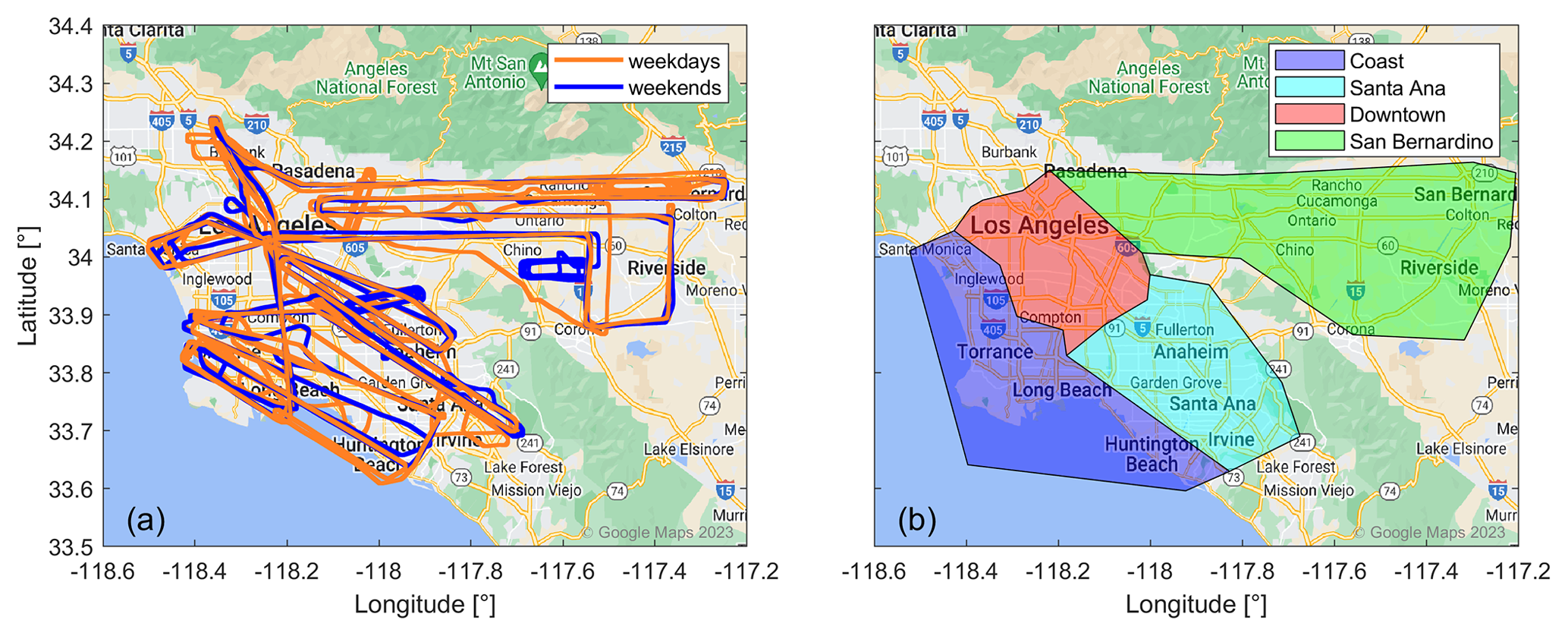
Figure 1(a) Overview of the flight paths during the RECAP-CA campaign over Los Angeles in June 2021. Blue colors show weekend flights and orange colors show weekday flights. (b) Geographic separation of the covered area into four segments, including the coast (blue), parts of Santa Ana county (light blue), Downtown Los Angeles (red) and the San Bernardino Valley (green). © Google Maps 2023.
2.2 Meteorological measurements
The meteorological instruments on board the CIRPAS Twin Otter research aircraft were previously described in Karl et al. (2013). Temperature was obtained by a Rosemount sensor (Emerson Electric Co., St. Louis, Missouri, USA). Dew point temperature was measured by a DewMaster Chilled Mirror Hygrometer (Edgetech Instruments Inc., Hudson, Massachusetts, USA). Differential and barometric pressure sensors (Setra Systems, Inc., Boxborough, Massachusetts, USA) were used to determine the pressure. GPS latitude, longitude, altitude, ground speed and track, as well as pitch, heading and roll angle were measured by a C-MIGITS (Miniature Integrated GPS (global positioning system) and INS (inertial navigation system) Tactical System) III (Systron, Inc., Canada). A radome flow angle probe provided the true air speed and the 3D wind. The planetary boundary layer height (PBLH) was determined from changes in water vapor and toluene concentrations, the dew point and temperature, which decrease rapidly at the boundary between the boundary layer and the free troposphere (Pfannerstill et al., 2023). The aircraft crossed the top of the PBL several times during each flight, thus providing these direct observations.
2.3 NOx measurements
NOx measurements were carried out using a custom-built three-channel thermal dissociation laser-induced fluorescence (TD-LIF) instrument with a detection limit of ∼ 15 pptv (parts per trillion by volume; 10 s; higher for higher-resolution data) and a precision (2σ) of <7 % (Thornton et al., 2000). The instrument is described in detail in Thornton et al. (2000), Day et al. (2002) and Sparks et al. (2019). Briefly, NO2 is excited in the first channel with a 532 nm Nd3+:YVO4 laser (Explorer One XP, Spectra-Physics). The fluorescence resulting from NO de-excitation is detected by a photomultiplier tube as a signal which is approximately proportional to the ambient NO2 mixing ratio. The proportionality arises because the fluorescence signal and the quenching of the fluorescence both scale with pressure. Calibration with an NO2 gas standard (5.5 ppm; Praxair Technology, Inc.) was performed once an hour. The instrument background was determined every 20 min, using scrubbed ambient air. NO is determined in the second channel through conversion to NO2 by adding excess ozone (O3). Reactive nitrogen species (NOy≡NOx, HNO3, HONO, RONO2, RO2NO2, etc.) were detected through thermal dissociation at ∼500 ∘C to NO2 in the third channel (Day et al., 2002). Ambient air was sampled at a flow rate of 6 L min−1, which was equally divided into the three instrument channels.
2.4 NOx flux calculations
The emission of a trace gas is characterized as a flux which is a mass emitted per area and time (e.g., mg m2 h−1). A flux F can be described as the covariance of the fluctuation in the vertical wind speed w′ and the fluctuation in the concentration of the trace gas of interest c′, as shown in Eq. (1).
Analyses of the covariance of winds and concentrations from tower-based or aircraft-based observations enable the determination of fluxes. With the eddy covariance (EC) method, the flux is directly calculated from the measurements as the mean of the product of the deviation of the vertical wind speed from the mean of the vertical wind speed and the deviation of the concentration analogously, as shown in Eq. (2) (e.g.,Schaller et al., 2017; Desjardins et al., 2021).
Requirements for accurate fluxes with EC are stationary conditions and a vertical homogeneously mixed boundary layer. Typically, an averaging time of at least 30 min is used to ensure that the full spectrum of eddies is sampled (Schaller et al., 2017; Desjardins et al., 2021). The 30 min long averaging time is easily implementable for stationary tower installments. For aircraft observations, the high aircraft velocity and the associated rapid geographical change are inconsistent with the stationary requirement. An alternative is the flux calculation via wavelet transformation. This approach does not require the assumption of stationary conditions, as it enables the determination of a flux localized both in time and frequency (Karl et al., 2013; Schaller et al., 2017). A discrete time series, such as the vertical wind speed or the concentration of an atmospheric trace gas is convolved with a wavelet function ψa,b(t), yielding the wavelet coefficient W(a,b), according to Eq. (3) (Torrence and Compo, 1998; Thomas and Foken, 2005; Schaller et al., 2017; Desjardins et al., 2021).
The function ψa,b(t), Eq. (4), a wavelet, scaled by a and shifted by b, controls the frequency and the time of the wavelet, respectively. In our study, we use the complex Morlet wavelet ψM, Eq. (5), which is the product of a sine and a Gaussian function, with ω0=6 and (Torrence and Compo, 1998; Metzger et al., 2013; Wolfe et al., 2018).
The expression represents the power spectrum of the discrete time series, showing each scale a and translation b with the applicable amplitude. For two different time series, the product of the wavelet coefficients yields the cross-power spectrum, which, when integrated across scales, represents the covariance and, in case of the vertical wind speed and the trace gas concentration, the flux (Torrence and Compo, 1998; Metzger et al., 2013; Schaller et al., 2017). The flux is calculated through wavelet transformation via Eq. (6).
Cδ is a reconstruction factor equal to 0.776 for the Morlet wavelet. N is the number of elements in the time series () with the time step δt. J is the number of scales () with the spacing δj (Metzger et al., 2013; Schaller et al., 2017; Desjardins et al., 2021). Both data pre-treatment (of the NOx and meteorological data) and wavelet analysis were performed by following the procedure presented by Vaughan et al. (2021). The time stamp of the meteorological data was interpolated to the NOx data time stamp, with a resolution of 5 Hz. We generated the flight segments as input for the wavelet analysis with a 10 km minimum length of continuous measurements. Observations above the boundary layer and thus in the free troposphere were excluded from our analysis, as they are assumed to be out of contact with the surface below. Data with an aircraft roll angle larger than 8∘, or where the altitude changed by more than ∼100 m across the 10 km, were excluded. Due to different inlet sampling locations and computer clocks, the NOx measurements and the vertical wind speed measurements were slightly time shifted. This lag correction was quantified via the cross-covariance of the two time series. The vertical wind speed was then shifted to the NOx measurements, according to the covariance peak. We used the median lag of all segments of the same flight day for the lag correction.
For the wavelet analysis, we followed the procedure described in detail in Torrence and Compo (1998). The wavelet transform was calculated separately for the vertical wind speed fluctuation w′ and the NOx concentration fluctuation c′. We used the wavelet software provided by Christopher Torrence and Gilbert P. Compo, with the Morlet wavelet ψM (described in Eq. 5), the time step δt=0.2 s−1, a scale spacing δj=0.25 and a scale number of (default value; ). For example, there would be 36 scales for a segment with 1000 data points. The cross-spectrum was obtained through the sum of the product of the real parts of the wavelet transform for c′ and w′ and the product of the imaginary parts, which gave the NOx flux via the weighted sum over all scales, according to Eq. (24) in Torrence and Compo (1998). Due to edge effects, the error is particularly high at the beginning and end of each segment, which is described by the cone of influence (COI; Torrence and Compo, 1998). We have discarded data points for which more than 80 % of the spectral information is located within the COI. Note that approximately 50 % of the data points are lost due to edge effects, likely due to short segment lengths and frequent calibrations. For our analysis, we used the 2 km moving mean of the NOx flux. Figure 2a shows the discrete time series of the NOx concentration and the vertical wind speed for one segment on 6 June, with a length of 30.0 km. The x axis shows the time in seconds from the start of the segment (∼9 min). Figure 2b shows the cross-power spectrum of c′ and w′, with red colors representing positive amplitudes and blue colors representing negative amplitudes; the COI is indicated by the dashed black line. The 2 km moving mean of the resulting NOx flux is presented in Fig. 2c.
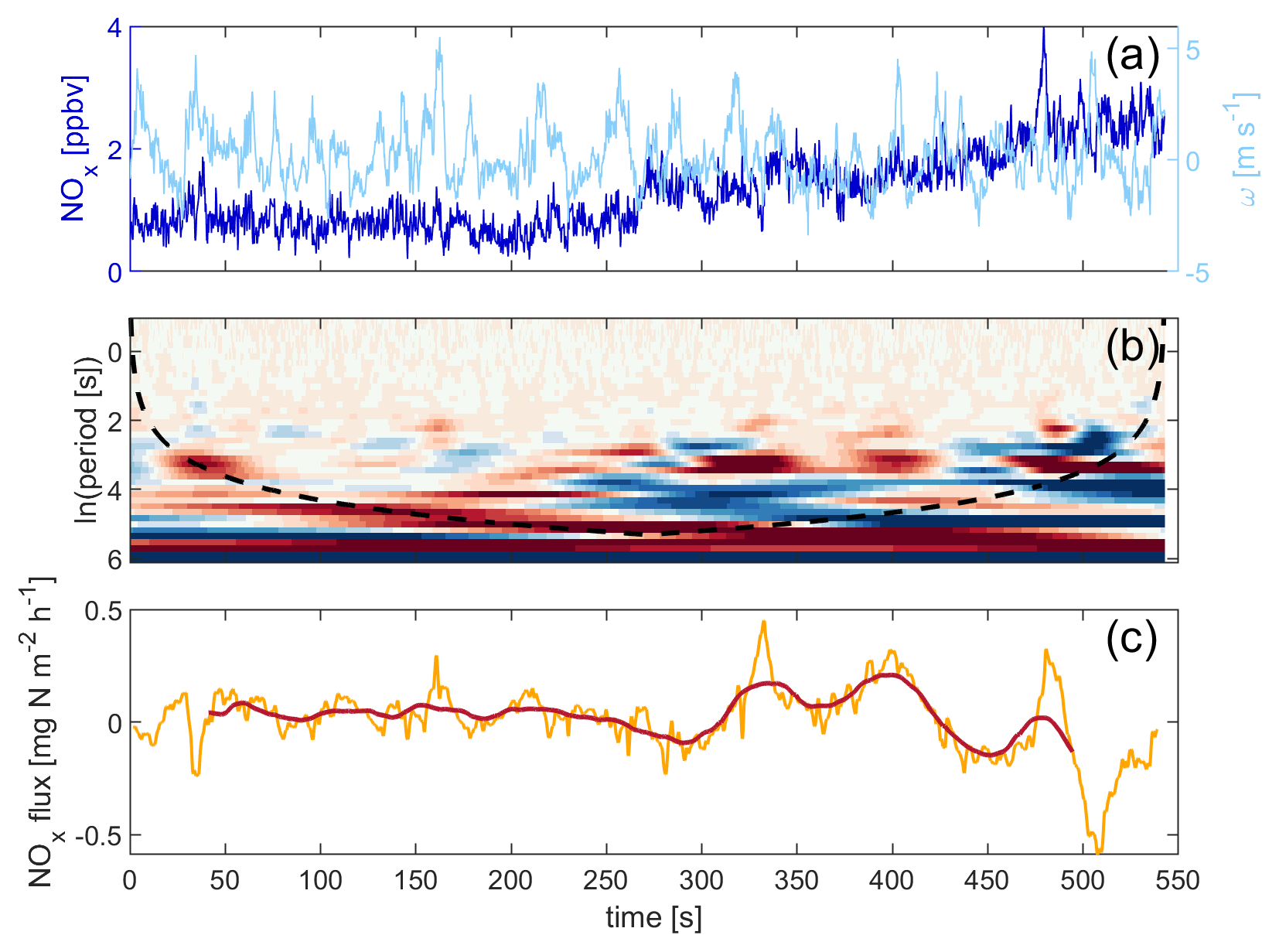
Figure 2(a) Discrete time series of the NOx concentration (dark blue) and the vertical wind speed (light blue) for a segment on 6 June. (b) Cross-power spectrum, with 41 scales and 2777 translations and the latter equaling the number of points in the segment. Red colors represent positive amplitudes, and blue colors represent negative amplitudes. (c) The resulting NOx flux (orange) and the 2 km moving mean (red) are shown.
In Fig. S2, we present an example covariance peak for NOx and potential temperature θ with the vertical wind speed, respectively, for three segments on 6 June. For all three segments shown here, the covariance for NOx and the vertical wind speed is clearly identifiable. The covariance peak for θ and the vertical wind speed can only be determined for two of these segments (middle and right panel). However, particularly for NOx, the identified lag times match quite well. As we expect the lag time to not vary throughout one flight (its variation is primarily associated with the alignment of different computer clocks and not the variation in the transit time to the detection point), we correct all segments with the median lag time of the identified segments. We show an example co-spectrum for the NOx flux and the heat flux in Fig. S3 for three segments on 6 June corresponding to Fig. S2. The Nyquist frequency, which is equal to half the sampling frequency, is shown as dotted black lines. We were able to capture most eddies due to the high sampling frequency of 5 Hz. Similar to the lag covariance, however, we observe difficulties for some of the segments. We explicitly chose positive and negative examples of lag covariance and co-spectra plots here to underline the strength and also the limitation of our data quality, which varies from segment to segment and is dependent on various factors, including the instrumental performance, meteorological conditions, the relative aircraft position within the boundary layer, the aircraft speed, the segment length, changes in altitude and the roll angle of the aircraft. A detailed error analysis and discussion can be found in Zhu et al. (2023).
The overall uncertainty of the calculated NOx flux is composed of the uncertainty in the measurement of the NOx concentration and the vertical wind speed. We find that the NOx median and average values are dominated by the atmospheric variability and not the measurement uncertainties. The observed atmospheric variability in NOx is on the order of 30 % (1σ), which is around 4 times higher than the instrumental precision of <7 % (1σ). Additional uncertainty is associated with the presented method of performing the wavelet transformation, including random and systematic errors (Lenschow et al., 1994; Mann and Lenschow, 1994; Wolfe et al., 2015; Vaughan et al., 2021). A detailed error analysis for these observations is provided in Zhu et al. (2023).
2.5 Vertical divergence
Vertical flux divergence describes the effect in which a flux measured at a certain altitude can differ from the surface flux caused, for example, through chemistry conversions, entrainment from above or horizontal advection (Wolfe et al., 2018; Vaughan et al., 2021). The characterization of the vertical divergence can be performed by measurements of a vertical profile over a homogeneous surface. Several racetracks stacked at multiple heights were conducted over Los Angeles during RECAP-CA, but none fulfilled the criteria for performing flux calculations, as described in Sect. 2.4 (e.g., roll angle or segment length). A different approach is described in Wolfe et al. (2018) and Zhu et al. (2023), which investigates the vertical profile of the calculated NOx fluxes that are normalized to the boundary layer height over a homogeneous surface. In contrast to San Joaquin Valley considered in Zhu et al. (2023), the measurements over Los Angeles are not homogeneous, neither in space nor in time, due to a high variety of emission sources and a diurnal cycle affected, e.g., by rush hour traffic. In Fig. S4, we show the calculated NOx flux across Los Angeles versus the dimensionless altitude , where z is the radar altitude of the research aircraft and zi the boundary layer height. Figure S5 presents the distribution of these data points as a density plot. The data points exhibit a decreasing trend (green) with altitude, pointing towards the effect of vertical divergence but show a low statistical significance with an R2 of only 6 %, likely due to the source heterogeneity, both space-wise and time-wise. In order to investigate the influence of vertical divergence, we compare an analysis with a correction of the fluxes, using the linear fit of the NOx flux (Fz) and the dimensionless altitude (), as shown in Fig. S4, to our analysis, assuming that the divergence is zero, which we will refer to as the sensitivity study in the following. We use a correction factor as presented in Eq. (15) in Wolfe et al. (2018). The uncertainty of this correction is dominated by the uncertainty in the fitted line, which arises from describing Fz vs. with a linear function, as presented in Fig. S4. The resulting surface flux F0 can then be calculated, as shown in Eq. (7), with the measured flux Fz at the altitude , the slope m of the linear fit and its y intercept c.
We show the fluxes adjusted for this estimate of the vertical divergence versus the dimensionless altitude in Fig. S6. Data points which are located close to the linear fit can be corrected quite accurately. However, corrections for data points which are located further away from the fit, and particularly those measured close to the boundary layer height (BLH), are highly uncertain. As the slope is negative, and the absolute values for slope and y intercept are almost equal, the denominator in Eq. (7) becomes extremely small close to the BLH, and the correction becomes correspondingly large. Karl et al. (2013) also suggest that fluxes can become uncertain close to the boundary layer height, due to entrainment to the free troposphere. Thus, for the sensitivity study, we omit data points within the upper 20 % of the boundary layer (), as a trade-off between high uncertainties close to the top of the PBL and the associated data loss. Additionally, the upper 20 % of the boundary layer were found to be most likely influenced by entrainment (Druilhet and Durand, 1984; Stull, 1988). The corrected fluxes filtered by the upper 20 % of the boundary layer are shown in Fig. S7.
2.6 Footprint calculations
In order to map emissions, we performed footprint calculations which help to identify the areas over which the associated sources and sinks influence the observed fluxes (Vesala et al., 2008). We used the footprint model KL04-2D, proposed by Kljun et al. (2004) and further developed by Metzger et al. (2012), to include the impact of crosswinds. The KL04 model was developed from the 3D backward Lagrangian model KL02 (Kljun et al., 2002). This model was previously applied by Vaughan et al. (2021). The resulting footprints during RECAP-CA over Los Angeles are presented in Fig. 3.
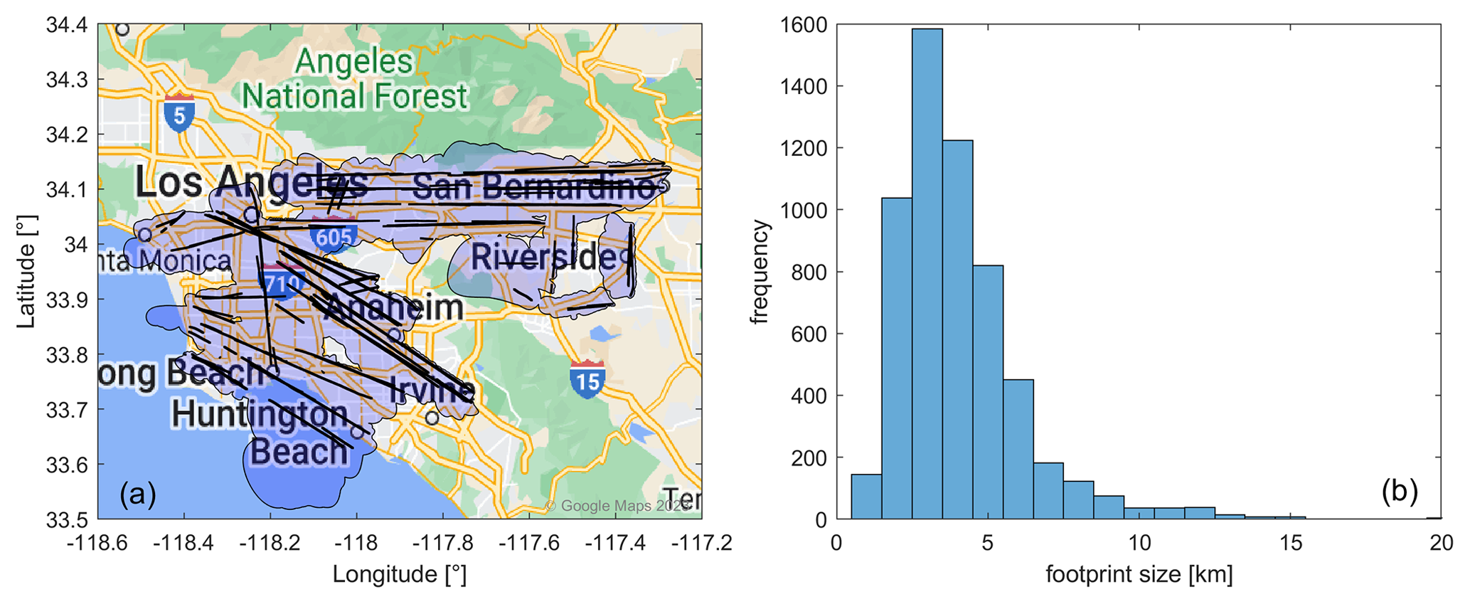
Figure 3(a) Overview of the 90 % footprint influences for the flight campaign over Los Angeles. © Google Maps 2023. (b) Frequency distribution of the 90 % footprint size, which describes the distance perpendicular to the flight track.
We subdivided the area of observations into a 500 m × 500 m spatial grid and calculated an average of all the data points located in one grid box separately for each segment. We then performed the footprint calculation for each grid box of each segment, generating approximately 5000 footprints for the entire campaign. The footprint calculation is dependent on the wind direction (∘), the crosswind fluctuations (standard deviation of the horizontal wind speed; m s−1), the vertical wind fluctuations (standard deviation of the vertical wind speed; m s−1), the friction velocity (m s−1), the roughness length (m), the altitude of the measurement above ground level (m) and the height of the planetary boundary layer (m). Please find details on the acquisition of the meteorological inputs in Sect. 2.2. The roughness length z0 is a measure of the surface properties, which we adapted from Burian et al. (2002) and from the World Meteorological Organization (2018), based on the land cover use for Los Angeles. We first generated footprints using the roughness length from the High-Resolution Rapid Refresh (HRRR) model by the National Oceanic and Atmospheric Administration (NOAA, 2021). Based on the dominant land cover type in each footprint, we then applied the roughness length according to Burian et al. (2002) and the World Meteorological Organization (2018). The land use data set was obtained from the Multi-Resolution Land Characteristics (MRLC) Consortium (MRLC, 2019). The friction velocity u* is a measure for the shear stress and can be approximated via the logarithmic wind profile, as shown in Eq. (8), where u is the horizontal wind speed, k the Karman constant equaling 0.41, z the altitude above ground level and z0 the roughness length (Weber, 1999).
The model output is a spatial grid of the fractional contribution to each footprint normalized to a value of unity. We focused on the 90 % footprint influences and assigned the measured NOx flux to the NOx flux of each grid box in the 90 % footprints. We then overlaid all footprint grids separately for weekends and for weekdays and calculated a value for the NOx flux for each grid box as the weighted average.
Figure 3a presents the 90 % contours of all segments over Los Angeles in blue and the respective flight paths in black. The majority of the 90 % footprints captured air masses from a distance of ∼3 km (perpendicular to the flight track), as shown in the histogram of the footprint size in Fig. 3b. We observed individual footprints with a size of up to 22.5 km, for example, for 19 June around Huntington Beach, which were accompanied by high horizontal wind speeds (∼5 m s−1) and a flight altitude (∼380 m) in the upper part of the boundary layer (BLH of ∼410 m). This is in line with the findings by Kljun et al. (2004) and demonstrates the impact of the receptor height (Fig. 1 in Kljun et al., 2004). The smallest footprint, with 500 m, was observed on 12 June and characterized by a small value for the horizontal wind speed, with ∼0.3 m s−1. The flight took place roughly in the middle of the boundary layer at an altitude of ∼315 m, with a BLH of ∼500 m.
The influence of the horizontal wind speed on the footprint analysis is also highlighted in Fig. 4. The two panels present selected flight segments colored by the NOx flux that is in geographic proximity over the San Bernardino Valley on 6 June (Fig. 4a) and on 12 June (Fig. 4b). Both days were weekend days, and we expect similar NOx emissions. However, the calculated NOx flux for the displayed segments was on average 0.08±0.09 mg N m−2 h−1 for 6 June and 0.53±0.34 mg N m−2 h−1 for 12 June. At the same time, the footprint size for these segments, represented by the black lines, was more than 4 times larger for 6 June, with an average of 7.1±2.5 km, than for 12 June, with an average of 1.9±1.0 km. The measured air on 12 June originated from above the highways in the San Bernardino Valley. In contrast, on 6 June we also captured air from adjacent sources with less NOx, such as residential areas, thus diluting the NOx polluted air from above the highways and leading to lower NOx fluxes. While all inputs for the footprint model were roughly similar (e.g., radar altitude 383 m for 6 June and 349 m for 12 June; BLH 637 m for 6 June and 600 m for 12 June), the horizontal wind speed was significantly higher on 6 June, with an average of 8.2±1.2 m s−1 than on 12 June, where the average was 2.5±1.0 m s−1. This example also underlines the importance of footprint calculations in the interpretation of the observed fluxes.
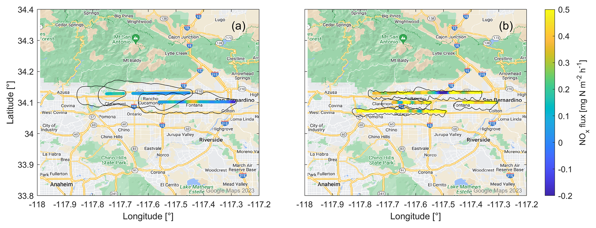
Figure 4Flight segments colored by the NOx flux in geographic proximity on 2 weekend days, (a) 6 June and (b) 12 June, with different footprint sizes. The black lines represent the contour of the 90 % footprints. © Google Maps 2023.
2.7 Emission inventory
The California Air Resources Board (CARB) provides an emission inventory for Los Angeles, with a 1 h temporal resolution and a 4 km × 4 km spatial resolution over 12 vertical layers. The emission inventory is assembled from several sub-models accounting for different emission source categories. These are on-road vehicle emissions, aircraft emissions and all other emissions, including, for example, shipping and port emissions. Mobile emissions are obtained via the ESTA (Emissions Spatial and Temporal Allocator) model (CARB, 2019). Emissions from vehicles, including passenger cars, buses and heavy-duty trucks, are estimated via the EMFAC (EMission FACtors) model, based on vehicle registrations and emission rate data for different vehicle types (CARB, 2021, 2022a). In combination with spatial information and temporal data, such as diurnal profiles and day-of-week dependence, the on-road emission inventory can be created via the ESTA model (CARB, 2019). The GATE (Gridded Aircraft Trajectory Emissions) model analogously provides spatially and temporally resolved aircraft emissions (CARB, 2017). Emissions from shipping and port activities, and additional point or area sources, are modeled with the SMOKE (Sparse Matrix Operator Kernel Emissions) model (CEMPD, 2022).
We are presenting a comparison of the NOx fluxes calculated from the RECAP-CA campaign measurements with the 2020 CARB emission inventory for Los Angeles, which is a baseline inventory and therefore does not include any effects related to the COVID-19 (coronavirus disease 2019) economic and social upheaval. For each flight day of the 2021 campaign, we include the corresponding day of the week of the emission inventory in 2020. As 2020 was a leap year, the day of year for each considered flight is shifted by two from the 2020 calendar (e.g., Tuesday, 1 June, was the 152nd day of 2021 for which we consider Tuesday, 2 June, the 154th day of 2020, from the emission inventory). We combined the 500 m × 500 m spatial resolution of the RECAP-CA NOx fluxes to the 4 km × 4 km CARB grid for this comparison.
3.1 NOx emissions over Los Angeles
NOx mixing ratios and NOx fluxes over Los Angeles are separated into four different geographical regions, as shown in Fig. 1b. We analyze the effects of temperature and the planetary boundary layer height, as well as differences between weekend and weekday data. Figure 5 shows the temperature for the different sections that were measured on the research aircraft (380±63 m altitude). The lowest temperatures were observed in the coastal section, with a median value of 17 ∘C. Temperatures measured over Santa Ana and Downtown Los Angeles were slightly higher, with median values around 19 ∘C. Further inland, observed temperatures were highest, with a median value of 24 ∘C. Differences between the four sections were also observed regarding the boundary layer height (BLH), as presented in Fig. 5b. The lowest BLH was found for the coastal section, with a median value of 470 m, followed by Santa Ana with 490 m and a median value of 540 m for Downtown Los Angeles. The BLH in the San Bernardino Valley was highest, with a median value of 590 m. Figure 5c shows NOx mixing ratios, and Fig. 5d shows the corresponding fluxes over Los Angeles separated into the geographical sections and into weekdays and weekends. Neither NOx mixing ratios nor NOx fluxes were found to be temperature dependent (see Fig. S8).
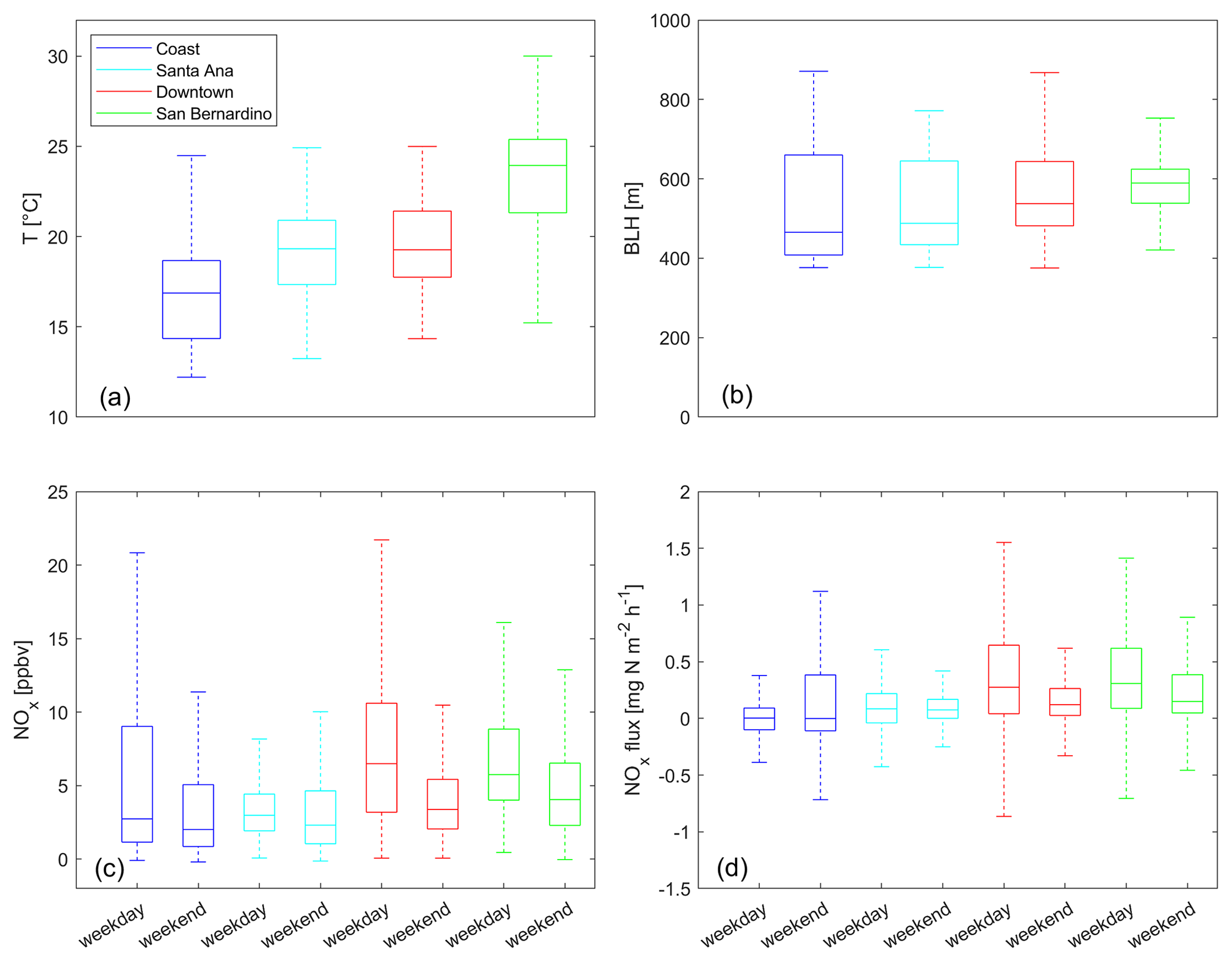
Figure 5Box plots for (a) the temperature, (b) the boundary layer height, (c) NOx concentrations and (d) NOx fluxes subdivided into four geographical sections, according to Fig. 1b (same color code), and into weekday and weekend data. Blue colors represent the coast, cyan colors the Santa Ana region, red colors Downtown Los Angeles and green colors the San Bernardino Valley. Please note that outliers are not shown.
Median mixing ratios were highest in Downtown Los Angeles, with 6.5 ppbv on weekdays and 3.4 ppbv on weekends. In the San Bernardino Valley, median concentrations were 5.8 and 4.1 ppbv on weekdays and weekends, respectively. The observed levels of NOx reductions from weekdays to weekends are consistent with previous results based on ground-based measurements across Los Angeles, which, for example, we have investigated in Nussbaumer and Cohen (2020). The median measured fluxes in Downtown Los Angeles were 0.27 and 0.12 mg N m−2 h−1, respectively, for weekdays and weekends. In the San Bernardino Valley, the median fluxes were 0.31 mg N m−2 h−1 on weekdays and 0.15 mg N m−2 h−1 on weekends. In all of these locations, weekend emissions decreased by 50 %–60 % from weekday values.
Mixing ratios were lower near the coast. Median NOx mixing ratios were similar for the coastal section and Santa Ana, with 2.8–3.0 ppbv on weekdays. The weekend values were smaller, with 2.0–2.3 ppbv. However, no significant differences could be observed between weekday and weekend fluxes in these regions. Much of the coastal region is over water, and the median values of fluxes are near-zero on both weekdays and weekends and approximately 0.1 mg N m−2 h−1 on both weekdays and weekends in the Santa Ana region.
While NOx concentrations were observed to be highest over Downtown Los Angeles, NOx fluxes were found to be highest in the San Bernardino Valley. This effect could be partly caused by the observed differences in the boundary layer height. While the highest emissions occurred in the San Bernardino Valley, the increased planetary BLH (as shown in Fig. 5b), should lead to a ∼15 % lower mixing ratio. The differences in concentrations are likely also due to chemistry and advection.
Using the highway information by the California Department of Transportation (2015), we separated NOx fluxes into emissions from highway and non-highway grid cells. A 500 m × 500 m grid cell is considered a highway emission when it is crossed by a highway. We present the resulting emission grid in Fig. S9. For weekdays, NOx fluxes from highway grid cells were on average 0.27±0.48 mg N m−2 h−1 and approximately 25 % higher than NOx fluxes from non-highway grid cells, with an average of 0.22±0.42 mg N m−2 h−1. Weekend NOx fluxes from highways were on average 0.19±0.31 mg N m−2 h−1. Weekend NOx emissions from non-highway areas were 0.15±0.32 mg N m−2 h−1. Note the large 1σ standard deviations, indicating the large variability in the fluxes. The median values were lower compared to the mean values (0.18 and 0.10 mg N m−2 h−1 for highway and non-highway, respectively, on weekdays and 0.09 and 0.13 mg N m−2 h−1 for highway and non-highway, respectively, on weekends) but showed a similar qualitative result with higher emissions from highway compared to non-highway areas.
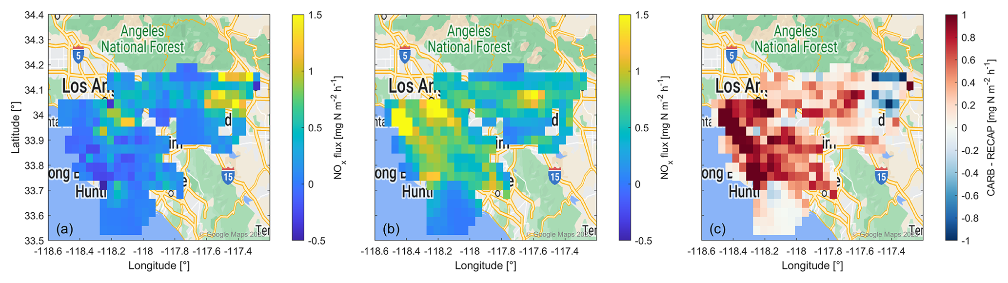
Figure 6Weekday averages of NOx emissions across Los Angeles, with a 4 km × 4 km spatial resolution (a) during the RECAP-CA campaign, (b) from the CARB emission inventory and (c) the difference between CARB and RECAP-CA NOx fluxes. © Google Maps 2023.
3.2 Comparison to the emission inventory
The comparison between the emission inventory and the calculated NOx fluxes is shown in Fig. 6. We present the weekday data here and show the weekend data in Fig. S10. This figure presents measured NOx fluxes, which are not corrected for vertical divergence. We present the results of the sensitivity study (as described in Sect. 2.5), applying a correction according to the linear fit presented in Fig. S4, and discuss the implications of this correction at the end of this section. Figure 6a shows the RECAP-CA NOx fluxes at 4 km × 4 km, Fig. 6b presents the CARB emission inventory, and in Fig. 6c we show the difference between the CARB and the RECAP-CA data. Red colors indicate higher fluxes from the emission inventory, and blue colors show higher fluxes from the RECAP-CA airborne measurements. As expected from the results presented in Sect. 3.1, the highest NOx fluxes were observed in the San Bernardino Valley, which is characterized by several heavily trafficked highways and warehouses that cause dense diesel truck traffic (Los Angeles Times, 2023). Elevated NOx emissions also occurred in the region around Downtown Los Angeles. The average weekend RECAP-CA NOx fluxes (Fig. S10a) showed a similar emission distribution over Los Angeles compared to the weekday data but with smaller values. This is in line with the findings presented in Sect. 3.1.
Figure 6b shows the average weekday NOx fluxes, as predicted by the CARB emission inventory. The large NOx flux in proximity to the coast (∼ 34.0∘ N, 118.4∘ W), with a value close to 3.5 mg N m−2 h−1, was associated with aircraft emissions and ground-handling equipment and vehicle traffic from and around Los Angeles International Airport (LAX). Additionally, emissions from aircraft not only at the surface but also at elevated altitudes could contribute to the observed value. We show the NOx fluxes, as predicted by CARB, separated into (a) on-road emissions, (b) aircraft emissions, (c) area sources (e.g., residential heating or cooking emissions which accumulate over a larger area; CARB, 2023) and (d) emissions from ocean-going vessels in Fig. S11. Aircraft NOx emissions can also be observed in the San Bernardino Valley (∼ 34.1∘ N, 117.6∘ W) from Ontario International Airport, which is illustrated in Fig. S11b. High NOx fluxes in this area were also associated with on-road emissions, as shown in Fig. S11a. The Downtown Los Angeles area (∼ 34.0∘ N, 118.2∘ W) also showed high fluxes which originated from on-road and area sources. Elevated NOx fluxes around Long Beach (∼ 33.8∘ N, 118.2∘ W) were associated with shipping and port emissions. Average weekend NOx fluxes predicted by the emission inventory are presented in Fig. S11b, which showed a similar qualitative distribution compared to the weekday data but were generally lower. Figure 6c presents the difference between the NOx fluxes from the RECAP-CA campaign and the CARB emission inventory. Blue colors represent higher values for the RECAP-CA campaign compared to the emission inventory. Red colors indicate higher fluxes from the emission inventory. In most places, the NOx fluxes predicted by the emission inventory were higher compared to the values from the RECAP-CA campaign. This difference was particularly pronounced in the area around Downtown Los Angeles and along the coast. Due to lively air traffic, the research aircraft could not approach the airport closely, and the footprints only covered a minor area of LAX airport. As a result, the differences in the vicinity of the airport should not be interpreted as meaningful. NOx fluxes around Downtown Los Angeles are dominated by area sources and on-road emissions.
We observed higher NOx fluxes during the RECAP-CA campaign compared to the emission inventory in the San Bernardino Valley. A possible explanation could be the accumulation of distribution and fulfillment centers which are accessible to delivery trucks via multiple highways in this area (Schorung and Lecourt, 2021; Los Angeles Times, 2023). Over the past 2 decades, net sales via distribution centers have grown exponentially (Statista, 2022a). In the USA, the number of delivered orders by the online retailer Amazon has increased by nearly a factor of 6 between 2018 and 2020 (Statista, 2022b). NOx emissions in proximity to warehouses have likely increased to a similar extent in recent years, which might not yet be incorporated in the CARB 2020 emission inventory. Additional research is needed to examine more details of these differences and connect them to specific processes in the inventory and observations.
In Figs. S12 and S13, we show the NOx fluxes corrected for vertical divergence, as presented in Sect. 2.5, in comparison to the CARB emission inventory for weekdays and weekends, respectively. The emission features shown in Fig. 6 for the RECAP-CA campaign are more pronounced after applying the factor for vertical correction. High emissions are observed over Downtown Los Angeles and the inland highways in San Bernardino, while the coastal region and Santa Ana show lower, and even negative, fluxes. As a result, CARB emissions remain dominant over RECAP-CA fluxes in the coastal region but are lower around Downtown Los Angeles and in San Bernardino. The median values of the corrected fluxes are around a factor of 3 higher compared to the non-corrected fluxes. The interquartile range increases by even more as a result of the large scatter induced by the correction (compare Figs. S6 and S7). We do not correct the fluxes for vertical divergence, as our data set does not provide a significant or unambiguous indication for its occurrence and extent. This is likely an outcome of the source heterogeneity experienced across Los Angeles, as most emissions are highly variable in time and space. In previous studies, the vertical divergence has been successfully characterized via the correlation of the flux and the dimensionless altitude over homogeneous surfaces, which is not applicable to Los Angeles. Instead, carefully planned stacked racetrack flights could provide insight into the vertical flux divergence. This sensitivity analysis emphasizes how important the characterization of the vertical flux divergence is and should be the subject of future studies.
In this study, we have investigated NOx fluxes via wavelet analysis, based on airborne observations of NOx concentrations and the vertical wind speed during the research aircraft campaign RECAP-CA, which took place in June 2021 over Los Angeles. We identified NOx concentrations to be highest over Downtown Los Angeles, while we found highest NOx fluxes in the San Bernardino Valley, where a high PBLH induced a higher dilution of the emitted NOx. Both NOx concentrations and NOx fluxes revealed a weekend effect, with higher values on weekdays due to more commuter traffic and more diesel trucks on roads, which was most pronounced over Downtown Los Angeles and the San Bernardino Valley. Footprint calculations revealed that the distance of the 90 % influence was on average 4 km upwind, whereby the horizontal wind speed played a dominant role in the footprint size. NOx emissions predicted by the California Air Resources Board (CARB) in 2020 were in the same order of magnitude but on average higher compared to the RECAP-CA NOx fluxes. Spatially, the emission inventory overestimated the fluxes in coastal proximity and over Downtown Los Angeles, which could be due to COVID-19-related reductions, such as a shift to more remote work and less commuter traffic, general emission reductions not yet captured by the emission inventory or the misallocation of emission sources in the inventory. In contrast, the emission inventory underestimated the NOx fluxes over the eastern part of the San Bernardino Valley, where an increased activity of trucks going to and from warehouses due to the exponential growth of online retailers, such as Amazon, have led to higher NOx emissions in recent years. A single uniform correction for vertical divergence could locally lead to improved agreement in this part of the domain but would at the same time increase the difference in other parts of the studied area. As this is an important tool in air quality regulation, we encourage further investigation of the accuracy of local emission inventories with observations from aircraft, towers or dense networks. For flux measurements from aircraft or towers, a particular focus on improving vertical divergence characterization, in order to provide accurate emission predictions, would be especially beneficial.
The codes used for the wavelet transformation and the footprint calculation are available at https://doi.org/10.5281/zenodo.8425485 (Zhu and Pfannerstill, 2023).
Data measured during the flight campaign, computed fluxes and footprints are available at https://doi.org/10.5281/zenodo.8199013 (Nussbaumer et al., 2023). Additional files, for example, in different resolutions, are available from the corresponding authors upon request.
The supplement related to this article is available online at: https://doi.org/10.5194/acp-23-13015-2023-supplement.
CMN analyzed the data, with contributions from BKP, QZ, and EYP. CMN wrote the paper. BKP, EYP, PW, BCS, CA, RW, AB, JHS, AHG, and RCC participated in the field campaign. All co-authors contributed to designing the study and proofreading the paper.
At least one of the (co-)authors is a member of the editorial board of Atmospheric Chemistry and Physics. The peer-review process was guided by an independent editor, and the authors also have no other competing interests to declare.
Publisher’s note: Copernicus Publications remains neutral with regard to jurisdictional claims made in the text, published maps, institutional affiliations, or any other geographical representation in this paper. While Copernicus Publications makes every effort to include appropriate place names, the final responsibility lies with the authors.
We acknowledge Horst Fischer and Lenard Röder for valuable discussions and proofreading this work. The wavelet software was provided by Christopher Torrence and Gilbert P. Compo and is available at http://paos.colorado.edu/research/wavelets/ (last access: 11 January 2022). Plots including Google Maps data were created with a MATLAB function by Bar-Yehuda (2022). This work has been supported by the Max Planck Graduate Center with the Johannes Gutenberg University Mainz (MPGC).
The RECAP-CA aircraft campaign has been funded by the California Air Resources Board (grant nos. 20RD003 and 20AQP012) and the South Coast Air Quality Management District (grant no. 20327).
The article processing charges for this open-access publication were covered by the Max Planck Society.
This paper was edited by Qi Chen and reviewed by Glenn Wolfe and one anonymous referee.
American Lung Association: Most Polluted Cities, https://www.lung.org/research/sota/city-rankings/most-polluted-cities (last access: 8 April 2022), 2022. a
Bar-Yehuda, Z.: zoharby/plot_google_map, https://github.com/zoharby/plot_google_map (last access: 11 July 2022), 2022. a
Boningari, T. and Smirniotis, P. G.: Impact of nitrogen oxides on the environment and human health: Mn-based materials for the NOx abatement, Curr. Opin. Chem. Eng., 13, 133–141, https://doi.org/10.1016/j.coche.2016.09.004, 2016. a
Burian, S. J., Brown, M. J., and Velugubantla, S. P.: Roughness length and displacement height derived from building databases, OSTI.GOV, https://www.osti.gov/biblio/976101 (last access: 6 October 2023), 2002. a, b
California Department of Transportation: State Highways (Segments), California, 2015, https://searchworks.stanford.edu/view/xc453kn9742 (last access: 15 July 2022), 2015. a
CARB: GATE Basic Introduction, GitHub, https://github.com/mmb-carb/GATE_Documentation/blob/master/docs/BASIC_INTRO.md (last access: 30 May 2022), 2017. a
CARB: ESTA Basic Introduction, GitHub, https://github.com/mmb-carb/ESTA_Documentation/blob/master/docs/BASIC_INTRO.md (last access: 30 May 2022), 2019. a, b
CARB: EMFAC2021 Volume III Technical Document, Tech. rep., Mobile Source Analysis Branch Air Quality Planning and Science Division, https://ww2.arb.ca.gov/sites/default/files/2021-08/emfac2021_technical_documentation_april2021.pdf?utm_medium=email&utm_source=govdelivery (last access: 31 May 2022), 2021. a
CARB: Welcome to EMFAC, https://arb.ca.gov/emfac/ (last access: 31 May 2022), 2022a. a
CARB: Nitrogen Dioxide and Health, https://ww2.arb.ca.gov/resources/nitrogen-dioxide-and-health (last access: 7 April 2022), 2022b. a, b
CARB: Criteria Pollutant Emission Inventory Data, https://ww2.arb.ca.gov/criteria-pollutant-emission-inventory-data (last access: 17 July 2023), 2023. a
CEMPD: SMOKE, GitHub, https://github.com/CEMPD/SMOKE/ (last access: 31 May 2022), 2022. a
Conley, S. A., Faloona, I., Miller, G. H., Lenschow, D. H., Blomquist, B., and Bandy, A.: Closing the dimethyl sulfide budget in the tropical marine boundary layer during the Pacific Atmospheric Sulfur Experiment, Atmos. Chem. Phys., 9, 8745–8756, https://doi.org/10.5194/acp-9-8745-2009, 2009. a
Day, D., Wooldridge, P., Dillon, M., Thornton, J., and Cohen, R.: A thermal dissociation laser-induced fluorescence instrument for in situ detection of NO2, peroxy nitrates, alkyl nitrates, and HNO3, J. Geophys. Res.-Atmos., 107, ACH 4-1–ACH 4-14, https://doi.org/10.1029/2001JD000779, 2002. a, b
Delmas, R., Serça, D., and Jambert, C.: Global inventory of NOx sources, Nutr. Cycl. Agroecosys., 48, 51–60, 1997. a
Desjardins, R. L., Worth, D. E., MacPherson, I., Mauder, M., and Bange, J.: Aircraft-Based Flux Density Measurements, in: Springer Handbook of Atmospheric Measurements, Springer International Publishing, Cham, 1305–1330, https://doi.org/10.1007/978-3-030-52171-4_48, 2021. a, b, c, d
Druilhet, A. and Durand, P.: Etude de la couche limite convective sahélienne en présence de brumes sèches (Expérience ECLATS), Bound.-Lay. Meteorol., 28, 51–77, https://doi.org/10.1007/BF00119456, 1984. a
Fujita, E. M., Campbell, D. E., Stockwell, W. R., and Lawson, D. R.: Past and future ozone trends in California's South Coast Air Basin: Reconciliation of ambient measurements with past and projected emission inventories, J. Air Waste Manage., 63, 54–69, https://doi.org/10.1080/10962247.2012.735211, 2013. a
Gu, D., Guenther, A. B., Shilling, J. E., Yu, H., Huang, M., Zhao, C., Yang, Q., Martin, S. T., Artaxo, P., Kim, S., Seco, R., Stavrakou, T., Longo, K. M., Tóta, J., de Souza, R. A. F., Vega, O., Liu, Y., Shrivastava, M., Alves, E. G., Santos, F. C., Leng, G., and Hu, Z.: Airborne observations reveal elevational gradient in tropical forest isoprene emissions, Nat. Commun., 8, 15541, https://doi.org/10.1038/ncomms15541, 2017. a
Hegg, D. A., Covert, D. S., Jonsson, H., and Covert, P. A.: Determination of the transmission efficiency of an aircraft aerosol inlet, Aerosol Sci. Tech., 39, 966–971, https://doi.org/10.1080/02786820500377814, 2005. a
Karl, T., Apel, E., Hodzic, A., Riemer, D. D., Blake, D. R., and Wiedinmyer, C.: Emissions of volatile organic compounds inferred from airborne flux measurements over a megacity, Atmos. Chem. Phys., 9, 271–285, https://doi.org/10.5194/acp-9-271-2009, 2009. a
Karl, T., Misztal, P., Jonsson, H., Shertz, S., Goldstein, A., and Guenther, A.: Airborne flux measurements of BVOCs above Californian oak forests: Experimental investigation of surface and entrainment fluxes, OH densities, and Damköhler numbers, J. Atmos. Sci., 70, 3277–3287, https://doi.org/10.1175/JAS-D-13-054.1, 2013. a, b, c, d
Kaser, L., Karl, T., Yuan, B., Mauldin III, R., Cantrell, C., Guenther, A. B., Patton, E., Weinheimer, A. J., Knote, C., Orlando, J., Emmons, L., Apel, E., Hornbrook, R., Shertz, S., Ullmann, K., Hall, S., Graus, M., de Gouw, J., Zhou, X., and Ye, C.: Chemistry-turbulence interactions and mesoscale variability influence the cleansing efficiency of the atmosphere, Geophys. Res. Lett., 42, 10894–10903, https://doi.org/10.1002/2015GL066641, 2015. a
Kljun, N., Rotach, M., and Schmid, H.: A three-dimensional backward Lagrangian footprint model for a wide range of boundary-layer stratifications, Bound.-Lay. Meteorol., 103, 205–226, https://doi.org/10.1023/A:1014556300021, 2002. a
Kljun, N., Calanca, P., Rotach, M., and Schmid, H.: A simple parameterisation for flux footprint predictions, Bound.-Lay. Meteorol., 112, 503–523, https://doi.org/10.1023/B:BOUN.0000030653.71031.96, 2004. a, b, c
Lenschow, D., Mann, J., and Kristensen, L.: How long is long enough when measuring fluxes and other turbulence statistics?, J. Atmos. Ocean. Tech., 11, 661–673, https://doi.org/10.1175/1520-0426(1994)011<0661:HLILEW>2.0.CO;2, 1994. a
Los Angeles Times: Warehouse boom transformed Inland Empire. Are jobs worth the environmental degradation?, https://www.latimes.com/california/story/2023-02-05/warehouses-big-rigs-fill-inland-empire-streets?utm_id=85748&sfmc_id=1882085 (last access: 6 March 2023), 2023. a, b
Mann, J. and Lenschow, D. H.: Errors in airborne flux measurements, J. Geophys. Res.-Atmos., 99, 14519–14526, https://doi.org/10.1029/94JD00737, 1994. a
Metzger, S., Junkermann, W., Mauder, M., Beyrich, F., Butterbach-Bahl, K., Schmid, H. P., and Foken, T.: Eddy-covariance flux measurements with a weight-shift microlight aircraft, Atmos. Meas. Tech., 5, 1699–1717, https://doi.org/10.5194/amt-5-1699-2012, 2012. a
Metzger, S., Junkermann, W., Mauder, M., Butterbach-Bahl, K., Trancón y Widemann, B., Neidl, F., Schäfer, K., Wieneke, S., Zheng, X. H., Schmid, H. P., and Foken, T.: Spatially explicit regionalization of airborne flux measurements using environmental response functions, Biogeosciences, 10, 2193–2217, https://doi.org/10.5194/bg-10-2193-2013, 2013. a, b, c
Mills, G., Pleijel, H., Malley, C. S., Sinha, B., Cooper, O. R., Schultz, M. G., Neufeld, H. S., Simpson, D., Sharps, K., Feng, Z., Gerosa, G., Harmens, H., Kobayashi, K., Saxena, P., Paoletti, E., Sinha, V., and Xu, X.: Tropospheric Ozone Assessment Report: Present-day tropospheric ozone distribution and trends relevant to vegetation, Elementa: Science of the Anthropocene, 6, 47, https://doi.org/10.1525/elementa.302, 2018. a
Misztal, P. K., Karl, T., Weber, R., Jonsson, H. H., Guenther, A. B., and Goldstein, A. H.: Airborne flux measurements of biogenic isoprene over California, Atmos. Chem. Phys., 14, 10631–10647, https://doi.org/10.5194/acp-14-10631-2014, 2014. a
MRLC: Multi-Resolution Land Characteristics (MRLC) Consortium – National Land Cover Database, https://www.mrlc.gov/ (last access: 2 May 2022), 2019. a
NOAA: The High-Resolution Rapid Refresh (HRRR), https://rapidrefresh.noaa.gov/hrrr/ (last access: 25 May 2022), 2021. a
Nussbaumer, C. M. and Cohen, R. C.: The Role of Temperature and NOx in Ozone Trends in the Los Angeles Basin, Environ. Sci. Technol., 54, 15652–15659, https://doi.org/10.1021/acs.est.0c04910, 2020. a, b
Nussbaumer, C. M., Place, B. K., Zhu, Q., Pfannerstill, E. Y., Wooldridge, P., Schulze, B. C., Arata, C., Ward, R., Bucholtz, A., Seinfeld, J. H., Goldstein, A. H., and Cohen, R. C.: Supporting data for: Measurement report: Airborne measurements of NOx fluxes over Los Angeles during the RECAP-CA 2021 campaign, Version 1, Zenodo [data set], https://doi.org/10.5281/zenodo.7786409, 2023. a
Nuvolone, D., Petri, D., and Voller, F.: The effects of ozone on human health, Environ. Sci. Pollut. R., 25, 8074–8088, https://doi.org/10.1007/s11356-017-9239-3, 2018. a
Pfannerstill, E. Y., Arata, C., Zhu, Q., Schulze, B. C., Woods, R., Seinfeld, J. H., Bucholtz, A., Cohen, R. C., and Goldstein, A. H.: Volatile organic compound fluxes in the San Joaquin Valley – spatial distribution, source attribution, and inventory comparison, EGUsphere [preprint], https://doi.org/10.5194/egusphere-2023-723, 2023. a
Pusede, S. E., Steiner, A. L., and Cohen, R. C.: Temperature and recent trends in the chemistry of continental surface ozone, Chem. Rev., 115, 3898–3918, https://doi.org/10.1021/cr5006815, 2015. a
Qian, Y., Henneman, L. R., Mulholland, J. A., and Russell, A. G.: Empirical development of ozone isopleths: Applications to Los Angeles, Environ. Sci. Tech. Let., 6, 294–299, https://doi.org/10.1021/acs.estlett.9b00160, 2019. a
Reid, J. S., Jonsson, H. H., Smith, M. H., and Smirnov, A.: Evolution of the vertical profile and flux of large sea-salt particles in a coastal zone, J. Geophys. Res.-Atmos., 106, 12039–12053, https://doi.org/10.1029/2000JD900848, 2001. a
Schaller, C., Göckede, M., and Foken, T.: Flux calculation of short turbulent events – comparison of three methods, Atmos. Meas. Tech., 10, 869–880, https://doi.org/10.5194/amt-10-869-2017, 2017. a, b, c, d, e, f
Schorung, M. and Lecourt, T.: Analysis of the spatial logics of Amazon warehouses following a multiscalar and temporal approach. For a geography of Amazon's logistics system in the United States, https://halshs.archives-ouvertes.fr/halshs-03489397/document (last access: 31 May 2022), 2021. a
South Coast Air Quality Management District: Final 2016 air quality management plan, Chap. 2, Tech. rep., South Coast Air Quality Management District, http://www.aqmd.gov/docs/default-source/clean-air-plans/air-quality-management-plans/2016-air-quality-management-plan/final-2016-aqmp/chapter2.pdf (last access: 8 April 2022), 2017. a
Sparks, T. L., Ebben, C. J., Wooldridge, P. J., Lopez-Hilfiker, F. D., Lee, B. H., Thornton, J. A., McDuffie, E. E., Fibiger, D. L., Brown, S. S., Montzka, D. D., Weinheimer, A. J., Schroder, J. C., Campuzano-Jost, P., Jimenez, J. L., and Cohen, R. C.: Comparison of airborne reactive nitrogen measurements during WINTER, J. Geophys. Res.-Atmos., 124, 10483–10502, https://doi.org/10.1029/2019JD030700, 2019. a
Statista: Annual net sales revenue of Amazon from 2004 to 2021, https://www.statista.com/statistics/266282/annual-net-revenue-of-amazoncom/ (last access: 1 June 2022), 2022a. a
Statista: Number of packages delivered by Amazon Logistics in the United States from 2018 to 2020 (in billion packages), https://www.statista.com/statistics/1178979/amazon-logistics-package-volume-united-states/ (last access: 1 June 2022), 2022b. a
Stewart, D. R., Saunders, E., Perea, R. A., Fitzgerald, R., Campbell, D. E., and Stockwell, W. R.: Linking air quality and human health effects models: an application to the Los Angeles air basin, Environmental Health Insights, 11, 1178630217737551, https://doi.org/10.1177/1178630217737551, 2017. a
Stull, R. B.: An introduction to boundary layer meteorology, Vol. 13, Springer Science & Business Media, https://doi.org/10.1007/978-94-009-3027-8, 1988. a
Thomas, C. and Foken, T.: Detection of long-term coherent exchange over spruce forest using wavelet analysis, Theor. Appl. Climatol., 80, 91–104, https://doi.org/10.1007/s00704-004-0093-0, 2005. a
Thornton, J. A., Wooldridge, P. J., and Cohen, R. C.: Atmospheric NO2: In situ laser-induced fluorescence detection at parts per trillion mixing ratios, Anal. Chem., 72, 528–539, https://doi.org/10.1021/ac9908905, 2000. a, b
Torrence, C. and Compo, G. P.: A practical guide to wavelet analysis, B. Am. Meteorol. Soc., 79, 61–78, https://doi.org/10.1175/1520-0477(1998)079<0061:APGTWA>2.0.CO;2, 1998. a, b, c, d, e, f
U.S. EPA: Overview of the Clean Air Act and Air Pollution, U.S. EPA, https://www.epa.gov/clean-air-act-overview (last access: 7 April 2022), 2022a. a
U.S. EPA: Air Data – Ozone Exceedances, U.S. EPA, https://www.epa.gov/outdoor-air-quality-data/air-data-ozone-exceedances (last access: 7 April 2022), 2022b. a
U.S. EPA: California Nonattainment/Maintenance Status for Each County by Year for All Criteria Pollutants, U.S. EPA, https://www3.epa.gov/airquality/greenbook/anayo_ca.html (last access: 8 April 2022), 2022c. a
Vaughan, A. R., Lee, J. D., Misztal, P. K., Metzger, S., Shaw, M. D., Lewis, A. C., Purvis, R. M., Carslaw, D. C., Goldstein, A. H., Hewitt, C. N., Davison, B., and Beeversh, Sean D. Karl, T. G.: Spatially resolved flux measurements of NOx from London suggest significantly higher emissions than predicted by inventories, Faraday Discuss., 189, 455–472, https://doi.org/10.1039/c5fd00170f, 2016. a
Vaughan, A. R., Lee, J. D., Metzger, S., Durden, D., Lewis, A. C., Shaw, M. D., Drysdale, W. S., Purvis, R. M., Davison, B., and Hewitt, C. N.: Spatially and temporally resolved measurements of NOx fluxes by airborne eddy covariance over Greater London, Atmos. Chem. Phys., 21, 15283–15298, https://doi.org/10.5194/acp-21-15283-2021, 2021. a, b, c, d, e
Vesala, T., Kljun, N., Rannik, Ü., Rinne, J., Sogachev, A., Markkanen, T., Sabelfeld, K., Foken, T., and Leclerc, M. Y.: Flux and concentration footprint modelling: State of the art, Environ. Pollut., 152, 653–666, https://doi.org/10.1016/j.envpol.2007.06.070, 2008. a
Weber, R. O.: Remarks on the definition and estimation of friction velocity, Bound.-Lay. Meteorol., 93, 197–209, https://doi.org/10.1023/A:1002043826623, 1999. a
Wolfe, G. M., Hanisco, T. F., Arkinson, H. L., Bui, T. P., Crounse, J. D., Dean-Day, J., Goldstein, A., Guenther, A., Hall, S. R., Huey, G., Jacob, D. J., Karl, T., Kim, P. S., Liu, X., Marvin, M. R., Mikoviny, T., Misztal, P. K., Nguyen, T. B., Peischl, J., Pollack, I., Ryerson, T., St. Clair, J. M., Teng, A., Travis, K. R., Ullmann, K., Wennberg, P. O., and Wisthaler, A.: Quantifying sources and sinks of reactive gases in the lower atmosphere using airborne flux observations, Geophys. Res. Lett., 42, 8231–8240, https://doi.org/10.1002/2015GL065839, 2015. a, b, c
Wolfe, G. M., Kawa, S. R., Hanisco, T. F., Hannun, R. A., Newman, P. A., Swanson, A., Bailey, S., Barrick, J., Thornhill, K. L., Diskin, G., DiGangi, J., Nowak, J. B., Sorenson, C., Bland, G., Yungel, J. K., and Swenson, C. A.: The NASA Carbon Airborne Flux Experiment (CARAFE): instrumentation and methodology, Atmos. Meas. Tech., 11, 1757–1776, https://doi.org/10.5194/amt-11-1757-2018, 2018. a, b, c, d
World Meteorological Organization: Guide to Instruments and Methods of Observation, Volume I – Measurement of Meteorological Variables, ISBN: 978-92-63-10008-5, 2018. a, b
Yu, H., Guenther, A., Gu, D., Warneke, C., Geron, C., Goldstein, A., Graus, M., Karl, T., Kaser, L., Misztal, P., and Bin, Y.: Airborne measurements of isoprene and monoterpene emissions from southeastern US forests, Sci. Total Environ., 595, 149–158, https://doi.org/10.1016/j.scitotenv.2017.03.262, 2017. a, b
Yuan, B., Kaser, L., Karl, T., Graus, M., Peischl, J., Campos, T. L., Shertz, S., Apel, E. C., Hornbrook, R. S., Hills, A., Gilman, J. B., Lerner, B. M., Warneke, C., Flocke, F. M., Ryerson, T. B., Guenther, A. B., and de Gouw, J. A.: Airborne flux measurements of methane and volatile organic compounds over the Haynesville and Marcellus shale gas production regions, J. Geophys. Res.-Atmos., 120, 6271–6289, https://doi.org/10.1002/2015JD023242, 2015. a
Zhu, Q. and Pfannerstill, E. Y.: qdzhu/FLUX: v2.0 qdzhu/FLUX: 2nd release, Version 2.0, Zenodo [code], https://doi.org/10.5281/zenodo.8425485, 2023. a
Zhu, Q., Place, B., Pfannerstill, E. Y., Tong, S., Zhang, H., Wang, J., Nussbaumer, C. M., Wooldridge, P., Schulze, B. C., Arata, C., Bucholtz, A., Seinfeld, J. H., Goldstein, A. H., and Cohen, R. C.: Direct observations of NOx emissions over the San Joaquin Valley using airborne flux measurements during RECAP-CA 2021 field campaign, Atmos. Chem. Phys., 23, 9669–9683, https://doi.org/10.5194/acp-23-9669-2023, 2023. a, b, c, d, e