Impact of chlorine ion chemistry on ozone loss in the middle atmosphere during very large solar proton events

Solar coronal mass ejections can accelerate charged particles, mostly protons, to high energies, causing solar proton events (SPEs). Such energetic particles can precipitate upon the Earth's atmosphere, mostly in polar regions because of geomagnetic shielding. Here, SPE-induced chlorine activation due to ion chemistry can occur, and the activated chlorine depletes ozone in the polar middle atmosphere. We use the state-of-the-art 1D stacked-box Exoplanetary Terrestrial Ion Chemistry (ExoTIC) model of atmospheric ion and neutral composition to investigate such events in the Northern Hemisphere (NH). The Halloween SPE that occurred in late October 2003 is used as a test field for our study. This event has been extensively studied before using different 3D models and satellite observations. Our main purpose is to use such a large event that has been recorded by the Michelson Interferometer for Passive Atmospheric Sounding (MIPAS) on the Environmental Satellite (ENVISAT) to evaluate the performance of the ion chemistry model. Sensitivity tests were carried out for different model settings with a focus on the chlorine species of HOCl and ClONO₂ as well as O₃ and reactive nitrogen, NO_y. The model simulations were performed in the Northern Hemisphere at a high latitude of 67.5^∘ N, inside the polar cap. Comparison of the simulated effects against MIPAS observations for the Halloween SPE revealed rather good temporal agreement, also in terms of altitude range for HOCl, O₃ and NO_y. For ClONO₂, good agreement was found in terms of altitude range. The model showed ClONO₂ enhancements after the peak of the event. The best model setting was the one with full ion chemistry where O(¹D) was set to photo-chemical equilibrium. HOCl and ozone changes are very well reproduced by the model, especially for nighttime. HOCl was found to be the main active chlorine species under nighttime conditions, resulting in an increase of more than 0.2 ppbv. Further, ClONO₂ enhancements of 0.2–0.3 ppbv have been observed during both daytime and nighttime. Model settings that compared best with MIPAS observations were applied to an extreme solar event that occurred in AD 775, presumably once in a 1000-year event. With the model applied to this scenario, an assessment can be made about what is to be expected at worst for the effects of a SPE on the middle atmosphere, concentrating on the effects of ion chemistry compared to crude parameterizations. Here, a systematic analysis comparing the impact of the Halloween SPE and the extreme event on the Earth's middle atmosphere is presented. As seen from the model simulations, both events were able to perturb the polar stratosphere and mesosphere with a high production of NO_y and HO_x. Longer-lasting and stronger stratospheric ozone loss was seen for the extreme event. A qualitative difference between the two events and a long-lasting impact on HOCl and HCl for the extreme event were found. Chlorine ion chemistry contributed to stratospheric ozone losses of 2.4 % for daytime and 10 % for nighttime during the Halloween SPE, as seen with time-dependent ionization rates applied to the model. Furthermore, while comparing the Halloween SPE and the extreme scenario, with ionization rate profiles applied just for the event day, the inclusion of chlorine ion chemistry added ozone losses of 10 % and 20 % respectively.

1 Introduction

High-energy particles (e.g. electrons and protons) that precipitate at high latitudes can alter the chemical composition of the atmosphere by different photo-chemical reactions. This mainly happens due to primary collision processes and subsequent ion and neutral chemistry reactions. Such reactions ordered by increasing energy are e.g. excitation, photo-dissociation, photo-ionization, and dissociative ionization. These particles can come from various sources in outer space, accelerated by different processes to different energies. They affect different altitude ranges of the atmosphere. Such sources are e.g. galactic cosmic rays (GCRs), with protons and heavier nuclei of energies ranging from hundreds of mega-electron volt to giga-electron volt; coronal mass ejections and SPEs with protons of energies (MeV to GeV); auroral electrons during sub-storms accelerated to energies from 10 keV to hundreds of kilo-electron volt; and medium- and high-energy electrons in the radiation belts to energies from tens of kilo-electron volt to the mega-electron-volt range. This study involves SPEs which can also induce geomagnetic disturbances in the Earth's magnetosphere, leading to energetic electron precipitation (EEP) events. Recent studies, such as Verronen et al. (2005), which studied energetic particle precipitation (EPP) events, found significant co-variability in mesospheric ozone with proton and electron fluxes. HNO₃ increases measured during SPEs cannot be reproduced using the standard parameterization of HO_x and NO_x production, while models considering D-region ion chemistry in detail agree with the observations (Verronen et al., 2016). This finding highlighted the need to improve ion chemistry modelling in the D region for altitudes below 90 km in the ionosphere (Funke et al., 2011) to capture the EPP ozone interaction. The HO_x and NO_x parameterization cannot reproduce the longer-term effects of ion chemistry on e.g. the reactive nitrogen partitioning, ozone, and dynamics of the middle atmosphere (Kvissel et al., 2012).

In the case of parameterized NO_x, NO is produced when N(²D) reacts with molecular oxygen, as shown in Reaction (R1) (Porter et al., 1976; Jackman et al., 2005). This reaction is a major source of NO in the stratosphere, mesosphere, and lower thermosphere (Rusch et al., 1981; Barth, 1992).

$$\begin{array}{}\text{(R1)}& \mathrm{N}\left({}^{\mathrm{2}}\mathrm{D}\right)+{\mathrm{O}}_{\mathrm{2}}⟶\mathrm{NO}+\mathrm{O}\left({}^{\mathrm{3}}\mathrm{P},{}^{\mathrm{1}}\mathrm{D}\right)\end{array}$$

NO can be destroyed by Reaction (R2), which is an effective loss mechanism for NO_x, also known as the scavenging reaction (Jackman et al., 2005)

$$\begin{array}{}\text{(R2)}& \mathrm{N}\left({}^{\mathrm{4}}\mathrm{S}\right)+\mathrm{NO}⟶{\mathrm{N}}_{\mathrm{2}}+\mathrm{O}.\end{array}$$

O₂ can also react with the ground state N(⁴S); i.e. it is temperature-dependent and is a major source of NO in the thermosphere above ∼120 km (Sinnhuber et al., 2012; Barth, 1992). The excited states of N form NO, while the ground state can destroy NO, which is relevant in the stratosphere, mesosphere, and lower thermosphere. The partitioning between the ground and excited states determines the amount of NO_x formed (Sinnhuber et al., 2012; Nieder et al., 2014), thereby making Reaction (R2) the driver of the parameterized NO_x. Thus, Reaction (R2) makes the difference between full ion chemistry and parameterized NO_x formation. The main processes responsible for the odd hydrogen (HO_x = H, OH, HO₂) formation during energetic particle precipitation events, along with the ion chemistry processes leading to its release, were considered by Solomon et al. (1981). They take place after the initial formation of ion pairs. Solomon et al. (1981) considered the ion chemistry processes leading to a release of HO_x during energetic particle precipitation events. They found that the main process responsible is the uptake of water vapour into large-cluster ions and the subsequent release of hydrogen during recombination reactions of these cluster ions. Large-cluster ions can then be formed by reaction pathways like the following (Sinnhuber et al., 2012):

$$\begin{array}{}\text{(R3)}& {\displaystyle }& {\displaystyle }{\mathrm{O}}_{\mathrm{2}}^{+}\left({\mathrm{H}}_{\mathrm{2}}\mathrm{O}\right)+{\mathrm{H}}_{\mathrm{2}}\mathrm{O}⟶{\mathrm{H}}_{\mathrm{3}}{\mathrm{O}}^{+}\left(\mathrm{OH}\right)+{\mathrm{O}}_{\mathrm{2}},\text{(R4)}& {\displaystyle }& {\displaystyle }{\mathrm{O}}_{\mathrm{2}}^{+}\left({\mathrm{H}}_{\mathrm{2}}\mathrm{O}\right)+{\mathrm{H}}_{\mathrm{2}}\mathrm{O}⟶{\mathrm{H}}^{+}\left({\mathrm{H}}_{\mathrm{2}}\mathrm{O}\right)+\mathrm{OH}+{\mathrm{O}}_{\mathrm{2}}.\end{array}$$

These protonized water cluster ions can then recombine with electrons to form H and OH.

$$\begin{array}{}\text{(R5)}& {\mathrm{H}}_{\mathrm{3}}{\mathrm{O}}^{+}\left(\mathrm{OH}\right)+e^{-}⟶{\mathrm{H}}_{\mathrm{2}}\mathrm{O}+\mathrm{H}+\mathrm{OH}\end{array}$$

Hydrogen and nitrogen radicals led to ozone destruction through catalytic cycles in the stratosphere and mesosphere. Different studies found ozone depletion in the mesosphere during SPEs, e.g. Weeks et al. (1972), who studied a large polar cap absorption event in 1969 that was explained as a result of the formation of odd hydrogen (Swider and Keneshea, 1973).

1.1 Hydrogen catalytic cycles

Catalytic cycles involving HO₂ are very important in the lower stratosphere (10–30 km). The fastest of these cycles is shown in Reactions (R6)–(R8).

$$\begin{array}{}\text{(R6)}& {\displaystyle }& {\displaystyle }\mathrm{OH}+{\mathrm{O}}_{\mathrm{3}}⟶{\mathrm{HO}}_{\mathrm{2}}+{\mathrm{O}}_{\mathrm{2}}\text{(R7)}& {\displaystyle }& {\displaystyle }{\mathrm{HO}}_{\mathrm{2}}+\mathrm{O}⟶\mathrm{OH}+{\mathrm{O}}_{\mathrm{2}}\text{(R8)}& {\displaystyle }& {\displaystyle }\mathrm{Net}:{\mathrm{O}}_{\mathrm{3}}+\mathrm{O}⟶{\mathrm{O}}_{\mathrm{2}}+{\mathrm{O}}_{\mathrm{2}}\end{array}$$

Another example of HO_x catalytic destruction cycles that is important in the middle and upper mesospheres (above 60 km) is shown in Reactions (R9) and (R10) (Bates and Nicolet, 1950). In every chain of Reactions (R9) and (R10), one molecule of O₃, O(³P), or O(¹D) is lost while reforming H and OH and thereby produces a net ozone loss (Reaction R11).

$$\begin{array}{}\text{(R9)}& {\displaystyle }& {\displaystyle }\mathrm{H}+{\mathrm{O}}_{\mathrm{3}}⟶\mathrm{OH}+{\mathrm{O}}_{\mathrm{2}}\text{(R10)}& {\displaystyle }& {\displaystyle }\mathrm{OH}+\mathrm{O}⟶\mathrm{H}+{\mathrm{O}}_{\mathrm{2}}\text{(R11)}& {\displaystyle }& {\displaystyle }\mathrm{Net}:{\mathrm{O}}_{\mathrm{3}}+\mathrm{O}⟶{\mathrm{O}}_{\mathrm{2}}+{\mathrm{O}}_{\mathrm{2}}\end{array}$$

1.2 Nitrogen catalytic cycle

In the lower stratosphere, ozone loss is mainly due to the catalytic cycle with NO_x governed by Reactions (R12) and (R13), in which case the loss of ozone is more persistent due to the longer lifetimes of NO_x.

$$\begin{array}{}\text{(R12)}& {\displaystyle }& {\displaystyle }\mathrm{NO}+{\mathrm{O}}_{\mathrm{3}}⟶{\mathrm{NO}}_{\mathrm{2}}+{\mathrm{O}}_{\mathrm{2}}\text{(R13)}& {\displaystyle }& {\displaystyle }{\mathrm{NO}}_{\mathrm{2}}+\mathrm{O}⟶\mathrm{NO}+{\mathrm{O}}_{\mathrm{2}}\text{(R14)}& {\displaystyle }& {\displaystyle }\mathrm{Net}:{\mathrm{O}}_{\mathrm{3}}+\mathrm{O}⟶{\mathrm{O}}_{\mathrm{2}}+{\mathrm{O}}_{\mathrm{2}}\end{array}$$

1.3 Chlorine catalytic cycles

The focus of this paper is the impact of charged chlorine species during a SPE. Negative chlorine species constitute a significant part of the total anions in the mesosphere (Chakrabarty and Ganguly, 1989; Fritzenwallner and Kopp, 1998). The chlorine-negative ion is an abundant ion of the lower D region during daytime and nighttime. Other D-region-negative ions like O${}_{\mathrm{2}}^{-}$, O⁻, CO${}_{\mathrm{3}}^{-}$, OH⁻, NO${}_{\mathrm{2}}^{-}$, and NO${}_{\mathrm{3}}^{-}$ can react with HCl to produce Cl⁻, which forms Cl⁻(X), where X = (HCl, H₂O, CO₂, and HO₂) (Kopp and Fritzenwallner, 1997). Cl⁻ and Cl⁻(H₂O) are the most abundant chlorine ions in the mesosphere, as indicated by previous studies for e.g. Chakrabarty and Ganguly (1989), Fritzenwallner and Kopp (1998), and Turco (1977). Both species can react with atomic hydrogen, re-releasing HCl and some of the recombination reactions of negative chlorine species with positive ions like H⁺-release Cl, ClO, ClNO₂, and Cl₂. Since the ion reactions are faster, the SPE impacts due to chlorine ion chemistry are expected to occur without any notable delay. The reactions involving charged and uncharged chlorine species along with the reaction rate coefficients are given in Table A1.

Apart from the NO_x and HO_x catalytic cycles, solar proton events can also affect stratospheric chlorine chemistry, but whether solar protons effectively activate or deactivate chlorine depends on the illumination conditions. The ion production rates increase during a SPE and influence the chemistry of both charged and uncharged chlorine species. The neutral compounds of chlorine can then contribute to ozone loss. The chlorine catalytic cycles of ozone destruction are very efficient around 40 km (Lary, 1997). SPE-induced changes in chlorine species can contribute to the short-term ozone depletion occurring after the SPE (von Clarmann et al., 2005). This influence is indirect and is mainly caused by NO_x and HO_x enhancements. The ClO_x ozone loss catalytic cycles with ClO photolysis are as follows.

$$\begin{array}{}\text{(R15)}& {\displaystyle }& {\displaystyle }\mathrm{ClO}+\mathrm{O}⟶\mathrm{Cl}+{\mathrm{O}}_{\mathrm{2}}\text{(R16)}& {\displaystyle }& {\displaystyle }\mathrm{Cl}+{\mathrm{O}}_{\mathrm{3}}⟶\mathrm{ClO}+{\mathrm{O}}_{\mathrm{2}}\text{(R17)}& {\displaystyle }& {\displaystyle }\mathrm{Net}:{\mathrm{O}}_{\mathrm{3}}+\mathrm{O}⟶{\mathrm{O}}_{\mathrm{2}}+{\mathrm{O}}_{\mathrm{2}}\end{array}$$

This is the main cycle responsible for ozone loss in the middle and upper stratosphere between 40 and 50 km (Daniel et al., 1999). O is formed by the photolysis of O₂ and O₃ and is available during daytime. The catalytic cycle involving hypochlorous acid (HOCl) and ClO acts as a link between chlorine and HO_x enhancements as a result of the SPEs (Reactions R19–R23) (Lary, 1997). HOCl can photolyse during daytime and the OH formed can react with O₃, reforming HO₂, Cl, and ClO and thereby recycling HOCl again through Reaction (R19). This cycle mainly plays a role in the sunlit polar lower stratosphere (Lary, 1997). Reactive Cl can also be formed via reaction of OH with HCl.

$$\begin{array}{}\text{(R18)}& {\displaystyle }& {\displaystyle }\mathrm{OH}+\mathrm{HCl}⟶{\mathrm{H}}_{\mathrm{2}}\mathrm{O}+\mathrm{Cl}\text{(R19)}& {\displaystyle }& {\displaystyle }\mathrm{ClO}+{\mathrm{HO}}_{\mathrm{2}}⟶\mathrm{HOCl}+{\mathrm{O}}_{\mathrm{2}}\text{(R20)}& {\displaystyle }& {\displaystyle }\mathrm{HOCl}+h\mathit{\nu }⟶\mathrm{Cl}+\mathrm{OH}\text{(R21)}& {\displaystyle }& {\displaystyle }\mathrm{Cl}+{\mathrm{O}}_{\mathrm{3}}⟶\mathrm{ClO}+{\mathrm{O}}_{\mathrm{2}}\text{(R22)}& {\displaystyle }& {\displaystyle }\mathrm{OH}+{\mathrm{O}}_{\mathrm{3}}⟶{\mathrm{HO}}_{\mathrm{2}}+{\mathrm{O}}_{\mathrm{2}}\text{(R23)}& {\displaystyle }& {\displaystyle }\mathrm{Net}:\mathrm{2}{\mathrm{O}}_{\mathrm{3}}⟶\mathrm{3}{\mathrm{O}}_{\mathrm{2}}\end{array}$$

von Clarmann et al. (2005) showed an enhancement of chlorine monoxide, ClO, and HOCl immediately after the SPE. They concluded that this was due to Reactions (R21) and (R19). During an SPE, HOCl and reactive Cl present in the stratosphere can react with OH and HO₂ respectively to form ClO. Other reactions of Cl with HO₂ and H₂O₂ can yield the production of HCl, which is the most important stratospheric reservoir species of Cl. Reactions (R24)–(R27) are relevant to the study in Sect. 4.

$$\begin{array}{}\text{(R24)}& {\displaystyle }& {\displaystyle }\mathrm{HOCl}+\mathrm{OH}⟶\mathrm{ClO}+{\mathrm{H}}_{\mathrm{2}}\mathrm{O}\text{(R25)}& {\displaystyle }& {\displaystyle }\mathrm{Cl}+{\mathrm{HO}}_{\mathrm{2}}⟶\mathrm{ClO}+\mathrm{OH}\text{(R26)}& {\displaystyle }& {\displaystyle }\mathrm{Cl}+{\mathrm{HO}}_{\mathrm{2}}⟶\mathrm{HCl}+{\mathrm{O}}_{\mathrm{2}}\end{array}$$

$$\begin{array}{}\text{(R27)}& \mathrm{Cl}+{\mathrm{H}}_{\mathrm{2}}{\mathrm{O}}_{\mathrm{2}}⟶\mathrm{HCl}+{\mathrm{HO}}_{\mathrm{2}}\end{array}$$

This is another effective ozone loss cycle involving SPE-induced NO_x enhancements between 15 and 40 km (Lary, 1997). ClO can react with nitric oxide (Reactions R28–R31), which is most important in the 15–50 km altitude range, as suggested by Farman et al. (1985). NO_x enhancements are also essential regarding the production of ClONO₂. López-Puertas et al. (2005) and von Clarmann et al. (2005) reported the first experimental confirmation of Reaction (R32) under SPE conditions. ClO reacts with nitrogen dioxide, NO₂, which is most efficient in the lower stratosphere, forming ClONO₂ (Reactions R32–R36).

$$\begin{array}{}\text{(R28)}& {\displaystyle }& {\displaystyle }\mathrm{ClO}+\mathrm{NO}⟶\mathrm{Cl}+{\mathrm{NO}}_{\mathrm{2}}\text{(R29)}& {\displaystyle }& {\displaystyle }{\mathrm{NO}}_{\mathrm{2}}+\mathrm{O}\left({}^{\mathrm{3}}\mathrm{P}\right)⟶\mathrm{NO}+{\mathrm{O}}_{\mathrm{2}}\text{(R30)}& {\displaystyle }& {\displaystyle }\mathrm{Cl}+{\mathrm{O}}_{\mathrm{3}}⟶\mathrm{ClO}+{\mathrm{O}}_{\mathrm{2}}\text{(R31)}& {\displaystyle }& {\displaystyle }\mathrm{Net}:\mathrm{O}\left({}^{\mathrm{3}}\mathrm{P}\right)+{\mathrm{O}}_{\mathrm{3}}⟶\mathrm{2}{\mathrm{O}}_{\mathrm{2}}\text{(R32)}& {\displaystyle }& {\displaystyle }\mathrm{ClO}+{\mathrm{NO}}_{\mathrm{2}}⟶{\mathrm{ClONO}}_{\mathrm{2}}\text{(R33)}& {\displaystyle }& {\displaystyle }{\mathrm{ClONO}}_{\mathrm{2}}+h\mathit{\nu }⟶\mathrm{Cl}+{\mathrm{NO}}_{\mathrm{3}}\text{(R34)}& {\displaystyle }& {\displaystyle }{\mathrm{NO}}_{\mathrm{3}}+h\mathit{\nu }⟶\mathrm{NO}+{\mathrm{O}}_{\mathrm{2}}\text{(R35)}& {\displaystyle }& {\displaystyle }\mathrm{Cl}+{\mathrm{O}}_{\mathrm{3}}⟶\mathrm{ClO}+{\mathrm{O}}_{\mathrm{2}}\text{(R36)}& {\displaystyle }& {\displaystyle }\mathrm{Net}:\mathrm{O}\left({}^{\mathrm{3}}\mathrm{P}\right)+{\mathrm{O}}_{\mathrm{3}}⟶\mathrm{2}{\mathrm{O}}_{\mathrm{2}}\end{array}$$

The present paper deals with changes in HOCl, ClONO₂, ozone, and NO_y occurring in the Northern Hemisphere at a high latitude of 67.5^∘ N during the Halloween SPE from mid-October to early November 2003, peaking around 28–29 October. The Halloween SPE was one of the largest SPEs in the satellite era and consisted of a series of solar flares and coronal mass ejections. Such large events mainly occur in the declining phase of the solar maximum. Changes in the composition of HOCl, ClONO₂, ozone, and NO_y species during the Halloween SPE were previously reported in Funke et al. (2011) and Jackman et al. (2008). Funke et al. (2011) used different models to investigate the SPE-induced changes, and Jackman et al. (2008) used version 3 of the Whole Atmosphere Community Climate Model (WACCM). Both studies were compared with the Michelson Interferometer for Passive Atmospheric Sounding (MIPAS) observations from the polar orbit Environmental Satellite (ENVISAT). Damiani et al. (2012) also looked at chlorine species (i.e. HOCl, ClONO₂, ClO, and HCl) using MLS and MIPAS data and version 4 of the WACCM model during SPEs of 17 and 20 January 2005. However, they did not consider the D-region ion chemistry. Here, we studied the temporal evolution of changes in the respective chemical constituents considering the D-region ion chemistry in the 1D stacked-box model, Exoplanetary Terrestrial Ion Chemistry (ExoTIC). The ion chemistry was implemented by Winkler et al. (2009), upon which ExoTIC is based.

In order to have a better comparison of ExoTIC simulations with MIPAS observations, we ensured that they are sampled inside the polar vortex. The polar vortex is a large circumpolar cyclone that is formed due to decreased solar insolation in the polar winter stratosphere as a manifestation of a strong meridional temperature gradient caused by a lack of high-latitude solar heating during polar night and dominates the dynamics (Harvey et al., 2015). The assumption is that the air inside the polar vortex is horizontally well mixed and separated from air masses outside the vortex. This allows us to simulate it in a 1D vertical model. The ionization during particle precipitation in the polar cap is also assumed to be inside the polar vortex, where NO_x is conserved, which makes it more comparable to the 1D model. The procedure is described in detail in Sect. 3.1.

The Halloween SPE is later compared with an exceptionally strong cosmic ray event that occurred in AD 775. It was derived from the historical records in radiocarbon ¹⁴C measured in tree ring archives and later confirmed by ¹⁰Be and ³⁶Cl cosmogenic nuclides. Although various scenarios were initially proposed, it is concluded now that the event was caused by solar energetic particles (Sukhodolov et al., 2017). ¹⁰Be and ¹⁴C implied that the event had a very hard spectrum and thereby very high-energy protons. It is the strongest solar energetic particle storm known for the last 11 millennia (the Holocene), serving as a likely worst-case scenario 40–50 times stronger than the largest directly observed event on 23 February 1956 (Usoskin et al., 2013). This event was transient, as estimated using the ratio of different cosmogenic isotopes (Mekhaldi et al., 2015).

This paper is organized as follows. Section 2 describes the ionization rates, model framework, simulations, and satellite observations used to evaluate the model. Section 3 presents the results of the model evaluation with MIPAS satellite observations. An overview of the changes in chlorine species, ozone, and NO_y induced by the SPE is presented. Section 4 presents a case study comparing model simulations of the Halloween SPE with the extreme solar event. Section 5 shows some results describing the impact of chlorine ion chemistry on ozone loss. In Sect. 6, a conclusion is provided to check whether the data are well understood, together with a summary of how our results compare to previous studies. Finally, an assessment is given of how further studies could improve our current knowledge on SPE-induced ozone loss due to chlorine ion chemistry.

Figure 1 Time-dependent and daily averaged ionization rates (IRs) from 25 October to 4 November 2003 obtained from the AISstorm model for a latitude of 67.5^∘ N (a). Mean IRs before the SPE (27–28 October) and in the SPE main phase (28–29 October) obtained from AISstorm and mean IRs of the extreme event for the same latitude of 67.5^∘ N (b).

2 Data and methods

2.1 Ionization rates

The ionization rates (IRs) used for the Halloween SPE were obtained from the Atmospheric Ionisation during Substorm (AISstorm) model, which is an enhanced version of the Atmospheric Ionisation Module Osnabrück (AIMOS) model (Wissing and Kallenrode, 2009). The AIMOS model computes ionization rates by precipitating electrons, protons, and alpha particles for the whole atmosphere based on particle flux measurements from Polar Operational Environmental Satellites (POES), Meteorological Operational satellites (Metop), and Geostationary Operational Environmental Satellites (GOES). The treatment of the electron fluxes is in the energy range 0.154–300 keV, with protons with an energy range of 0.154 eV–500 MeV. In the AIMOS v2.0–AISstorm model, both the time resolution (0.5 h) and the spatial resolution have been improved compared to AIMOS. For a comparison of the model results with MIPAS observations, the time-dependent ionization rates were put into ExoTIC. Figure 1 on the left-hand side shows the temporal evolution of an ion pair's production rates for protons, electrons, and alpha particles, varying over the time period 25 October–4 November 2003 from the AISstorm model. These IRs are averaged over the longitudes for the latitude of 67.5^∘ N in the polar cap region and are also daily averaged. For the extreme event, integrated ionization rates were taken from an extreme SPE of 23 February 1956 (SPE 56) (Meyer et al., 1956), which was the strongest observed event with ground-level enhancement (GLE), > 4000 %. Cliver et al. (2022) estimated this factor to be 70 times the particle influence compared to the 1956 event, and the ionization rates were scaled accordingly. This factor was a rough estimate to scale the fluxes of particles and excess radiation such that the energy spectrum of SPE 56 was comparable to the isotope signals of the extreme event. Figure 1 on the right shows the ionization rate profiles for both events. The profiles for the Halloween SPE show the average IRs for 27 October (day 301) and 28 October (day 302) before the SPE (in blue) and the average IRs for 28 and 29 October during the main SPE phase (in green). It can be observed that the ionization rates for the stratosphere and lower mesosphere in the case of the extreme event are about 1–2 orders of magnitude higher compared to the Halloween SPE main phase. This is because the extreme event contained protons of energies up to a few giga-electron-volt protons compared to about only a few mega-electron-volt protons for the Halloween SPE, and the ionization rates for the same can be seen to reach much further down to the surface.

2.2 Description of the 1D model and experiments

ExoTIC is a 1D stacked-box model of the atmospheric neutral and ion composition (Herbst et al., 2022). The ion chemistry is based on the UBIC (University of Bremen ion chemistry) model developed by Winkler et al. (2009) for the terrestrial middle atmosphere. The neutral chemistry is based on the SLIMCAT (Single Layer Isentropic Model of Chemistry and Transport) model by Chipperfield (1999). It accounts for photo-ionization of NO by Lyman-α radiation, photo-dissociation of charged species, and photo-detachment of electrons but does not contain any diffusion or horizontal and vertical transport. It first simulates a neutral atmosphere and contains the time evolution of 106 charged and 58 neutral species that interact due to neutral, neutral–ion, and ion–ion gas-phase reactions as well as photolysis and photo-electron attachment and detachment reactions (Sinnhuber et al., 2012). The ExoTIC model extends the applicability of UBIC to atmospheres of (rocky) planets other than Earth with a wide range of orbital parameters, stellar systems, and base compositions as discussed by Herbst et al. (2019). More neutral species have been added to the ion chemistry in ExoTIC since the study by Winkler et al. (2009). The ionization of CO₂ was recently included. Another small change is that the equilibrium is calculated for the ions, which stabilized the model. The model contains boxes of 2.7 km, each in height. For the studies performed here, the background atmosphere was taken from the EMAC (ECHAM5 with MESSy Atmospheric Chemistry) atmospheric chemistry-climate model with T42 horizontal truncation. It has 74 levels in the vertical direction and covers an altitude of up to 200–220 km, depending on latitude and season, with a vertical resolution of 2.7 km. The neutral chemistry and the ion chemistry model are calculated iteratively as follows.

1. The neutral model is time-dependent and calculates the volume-mixing ratios of the neutral species with a variable time step and feeds them to the ion chemistry model.

2. The ion chemistry in the equilibrium state is calculated, calling it hourly from the neutral model. The highest level for which the ion chemistry is calculated is 1 (207.4 km), and the lowest level is 53 (25.4 km), which depends on the initialization.

3. The net effective production or loss rates of neutral species due to primary ionization and positive and negative ion chemistry, which can also be used as a parameterization for global chemistry-climate models (Nieder et al., 2014), are computed using an iterative chemical equilibrium approach.

4. The production rates resulting from the ion chemistry computation are then fed back to the 1D neutral chemistry model, which solves for the neutral atmospheric state transiently using the net effective production or loss reactions as well as neutral photo-chemistry reactions.

5. Lastly, this state is again returned to the ion chemistry model for the following computation.

The model settings used for the sensitivity studies were mainly variations of full ion chemistry containing both positive and negative ions from the D region, setting reactive O(¹D) in photo-chemical equilibrium and switching off the chlorine ion chemistry. Parameterized NO_x and HO_x model simulations based on Porter et al. (1976) and Solomon et al. (1981) were also carried out to assess the performance of the ion chemistry model.

2.2.1 Ion chemistry

The ionization in this case is driven by prescribed ionization rates and by photo-ionization of NO, with the primary positive charges being distributed onto N₂, N, O₂, and O balanced with electrons (Sinnhuber et al., 2012). These rates of the primary ions are calculated by ionization cross sections based on Rusch et al. (1981) and Jones and Rees (1973). All of the processes like dissociation and dissociative ionization of O₂ and N₂ as well as ionization of O₂, N₂, and O can form the excited states of N, O, N${}_{\mathrm{2}}^{+}$, N⁺, and NO⁺, which are also included in the model. More details with a full list of the reactions, reaction rates, and references for the reaction rates used for the positive ion chemistry can be found in Sinnhuber et al. (2012), and the newer versions can be found in Herbst et al. (2022).

The simulation results are sensitive to the changes in the O(¹D) branching ratio, $\mathit{\beta }=\mathrm{\Delta }\mathrm{O}\left({}^{\mathrm{1}}\mathrm{D}\right)/\left(\mathrm{\Delta }\mathrm{O}\right({}^{\mathrm{1}}\mathrm{D})+\mathrm{\Delta }\mathrm{O}({}^{\mathrm{3}}\mathrm{P}\left)\right)$, which is discussed in Winkler et al. (2009). Winkler et al. (2011) reported the O(¹D) corrections in the UBIC model in more detail. O(¹D) is a reactive species which is formed from the dissociation of O₂ and CO₂ by particle impact ionization but also in the ion chemistry reactions themselves. This generally goes into photo-chemical equilibrium, but this is not considered in the ion chemistry part of the model, so the rate of O(¹D) formation passed to the neutral chemistry is too large. There are a few other short-lived neutral species in the ion chemistry model, like the excited states of N, e.g. N(²D), which are treated like ions. Basically, O(¹D) is produced through Reaction (R1). Since O(¹D) is mostly short-lived but is not considered to go into equilibrium in the ion chemistry stage, a large rate of formation of O(¹D) is produced and is added to the neutral chemistry. The time constants for the quenching O(¹D) + M ⟶ O(³P) + M in the stratosphere are significantly smaller than the chosen integration time step in the ion chemistry model, which was also reported in Winkler et al. (2011). This causes too high O(¹D) concentrations and an unrealistically strong effect through Reaction (R37). O(¹D) can react with species like H₂O, H₂, and CH₄ in the lower stratosphere and also with HCl in the stratosphere to produce OH. Therefore, either setting the formation rates of O(¹D) to zero or calculating them in photo-chemical equilibrium can make a difference to the full ion chemistry through Reactions (R37)–(R40).

$$\begin{array}{}\text{(R37)}& {\displaystyle }& {\displaystyle }\mathrm{O}\left({}^{\mathrm{1}}\mathrm{D}\right)+{\mathrm{H}}_{\mathrm{2}}\mathrm{O}⟶\mathrm{2}\mathrm{OH}\text{(R38)}& {\displaystyle }& {\displaystyle }\mathrm{O}\left({}^{\mathrm{1}}\mathrm{D}\right)+{\mathrm{H}}_{\mathrm{2}}⟶\mathrm{OH}+\mathrm{H}\text{(R39)}& {\displaystyle }& {\displaystyle }\mathrm{O}\left({}^{\mathrm{1}}\mathrm{D}\right)+{\mathrm{CH}}_{\mathrm{4}}⟶{\mathrm{CH}}_{\mathrm{3}}+\mathrm{OH}\text{(R40)}& {\displaystyle }& {\displaystyle }\mathrm{O}\left({}^{\mathrm{1}}\mathrm{D}\right)+\mathrm{HCl}⟶\mathrm{OH}+\mathrm{Cl}\end{array}$$

2.2.2 Sensitivity tests switching off the chlorine ion chemistry

The purpose of this sensitivity test is to study the impact of the chlorine ion. We wanted to study what difference it makes to the full ion chemistry with a focus on the ozone loss. This is done by switching off the reactions of negative chlorine ions with neutrals or the recombination reactions with H⁺ in ExoTIC. The relevant reactions are given in Table A1.

2.2.3 Parameterized NO_x and HO_x

The assumption in the case of parameterized NO_x is that 1.25 N atoms are produced per ion pair when electrically charged particles collide and dissociate N₂. This process produces N${}_{\mathrm{2}}^{+}$ and NO⁺ ions and, finally, atomic nitrogen. The latter is produced in its ground state N(⁴S) (45 % or 0.55 per ion pair) and the excited state N(²D) (55 % or 0.7 per ion pair). These values are mostly used in the stratospheric and mesospheric models. In the case of HO_x, each ion pair typically results in the production of around two HO_x constituents, i.e. a pair of H and OH per ion pair during recombination of the protonized water cluster ions in the upper stratosphere and lower mesosphere (Reaction R5), which was first estimated by Swider and Keneshea (1973). Andersson et al. (2016) calculated the parameterized HO_x production using a fixed H₂O profile. In contrast, ExoTIC assumes a zero abundance of water vapour above 80 km, while below, water vapour is modelled as a pair of H and OH. The HO_x formation stops when there is no more water vapour. For high water vapour, two HO_x constituents per ion pair are formed, but the rate decreases with decreasing H₂O. As the H₂O profile used in Andersson et al. (2016) decreases strongly above 80 km, the rate of HO_x production also goes to zero above 80 km. Jackman et al. (2005) also considered this, and an ion pair is computed to produce less than two HO_x constituents per ion pair in the middle and upper mesosphere. In ExoTIC, two HO_x constituents are produced per ion pair everywhere, but the production of HO_x is balanced by loss of water vapour, and the production therefore stops when all water vapour is consumed, effectively also reducing the amount of HO_x production in regions of low water vapour. We choose two HO_x molecules per ion pair because we want to mainly concentrate on the middle mesosphere to the stratosphere and not the upper mesosphere, i.e. above 80 km.

2.3 MIPAS on ENVISAT

MIPAS was a Fourier transform spectrometer for the detection of mid-infrared limb emission spectra in the middle and upper atmosphere on the ENVISAT (Fischer et al., 2000) mission (Fischer et al., 2008). ENVISAT was launched in 2002 into a sun-synchronous polar orbit (800 km) and stopped operation in April 2012. The atmospheric spectra were inverted into vertical profiles of atmospheric pressure, temperature, and volume-mixing ratios (vmrs) of more than 30 trace constituents. MIPAS observed a spectral range of 4.15 to 14.6 µm with a high spectral resolution, where a wide variety of trace gases have absorption lines and signals that are generally higher than in other parts of the spectrum. This is because the Planck function maximizes at about 10 µm for atmospheric temperatures. The measurement strategy of the MIPAS instrument was based on trace gases with characteristic emission and absorption lines, represented by their absorption coefficients, which are unambiguous “fingerprints” of the particular trace gases. The MIPAS mission is separated into two phases, caused by a malfunction of the instrument around March 2004. The first phase of the mission (2002–2004) is usually referred to as the MIPAS full-resolution (FR) period. After the malfunction, operation was resumed with a reduced optical path difference, resulting in a deteriorated spectral resolution. The second phase starting in January 2005 is called the reduced-resolution (RR) period. Because of the long optical path through the atmospheric layers, MIPAS could also detect trace gases with very low mixing ratios. Vertical information was gained by scanning the atmosphere at different elevation angles with different tangent altitudes. MIPAS could observe atmospheric parameters in the altitude range from 5 to 68 km nominally with minimum and maximum vertical steps of 1 and 8 km respectively. The MIPAS data are used here for evaluation of the model results with different parameterizations. Data presented here are IMK version V5 data for HOCl, ozone, ClONO₂, and NO_y species (NO, NO₂, HNO₃, and N₂O₅) that are updates of those published by von Clarmann et al. (2006, 2012), Glatthor et al. (2006), Höpfner et al. (2007), and Funke et al. (2005).

2.3.1 Averaging kernels

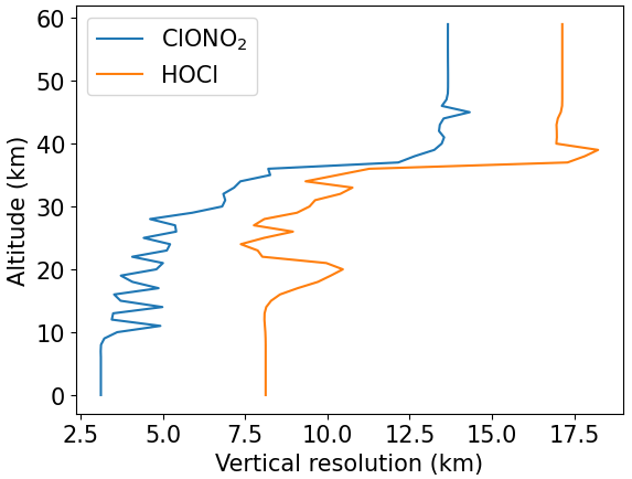
Different vertical resolutions of the MIPAS observations and the model need to be taken into account for a meaningful comparison. The ExoTIC model has a vertical resolution of 2.7 km, whereas MIPAS has different vertical resolutions for different species. For example, in the case of HOCl, the maximum vertical resolution can be 17 km, and for ClONO₂, it can be 13 km at an altitude of 40 km and above, as seen from an example in Fig. 2 for a specific time point.

Figure 2 Example of typical profiles for the vertical resolution of HOCl and ClONO₂.

To remove the discrepancy of different vertical resolutions between the model and MIPAS observations, the original model profiles have to be convolved and adjusted to the MIPAS altitude resolution. This adjustment procedure yields new species profiles that MIPAS would see if it were to sound the model atmosphere. For this purpose, we make use of the averaging kernels Rodgers (2000) and use a scheme suggested by Connor et al. (1994) to adjust the better-resolved model profiles to those of MIPAS, and the new adjusted model profiles x_new are calculated as

$$\begin{array}{}\text{(1)}& {\mathit{x}}_{\mathrm{new}}=\mathbf{A}{\mathit{x}}_{\mathrm{orig}}+(\mathbf{I}-\mathbf{A}){\mathit{x}}_{\mathrm{a}},\end{array}$$

where A is the MIPAS averaging kernel matrix, x_orig is the original model profile, I is a unity matrix, and x_a is the a priori information used in the MIPAS retrievals. The rows of the averaging kernel matrix give the contribution of the true values to the retrieved values and the columns give the response of the delta peak-like perturbations at each altitude. Figure 3 shows an example of averaging kernels for the different species and for a profile retrieved from spectra measured at a latitude of 67.5^∘ N on 27 October 2003 at 00:00 UT. From the figure, it is seen that the trace gas retrievals result in different sensitivities at different altitudes. For example, the maximum sensitivity is seen at 20 km for HOCl in this specific case, whereas, for ClONO₂, it is around 15 km. To characterize the vertical resolution, the typical measures are either the full width at half-maximum of the rows of the A or the grid width divided by the respective diagonal of A (Rodgers, 2000).

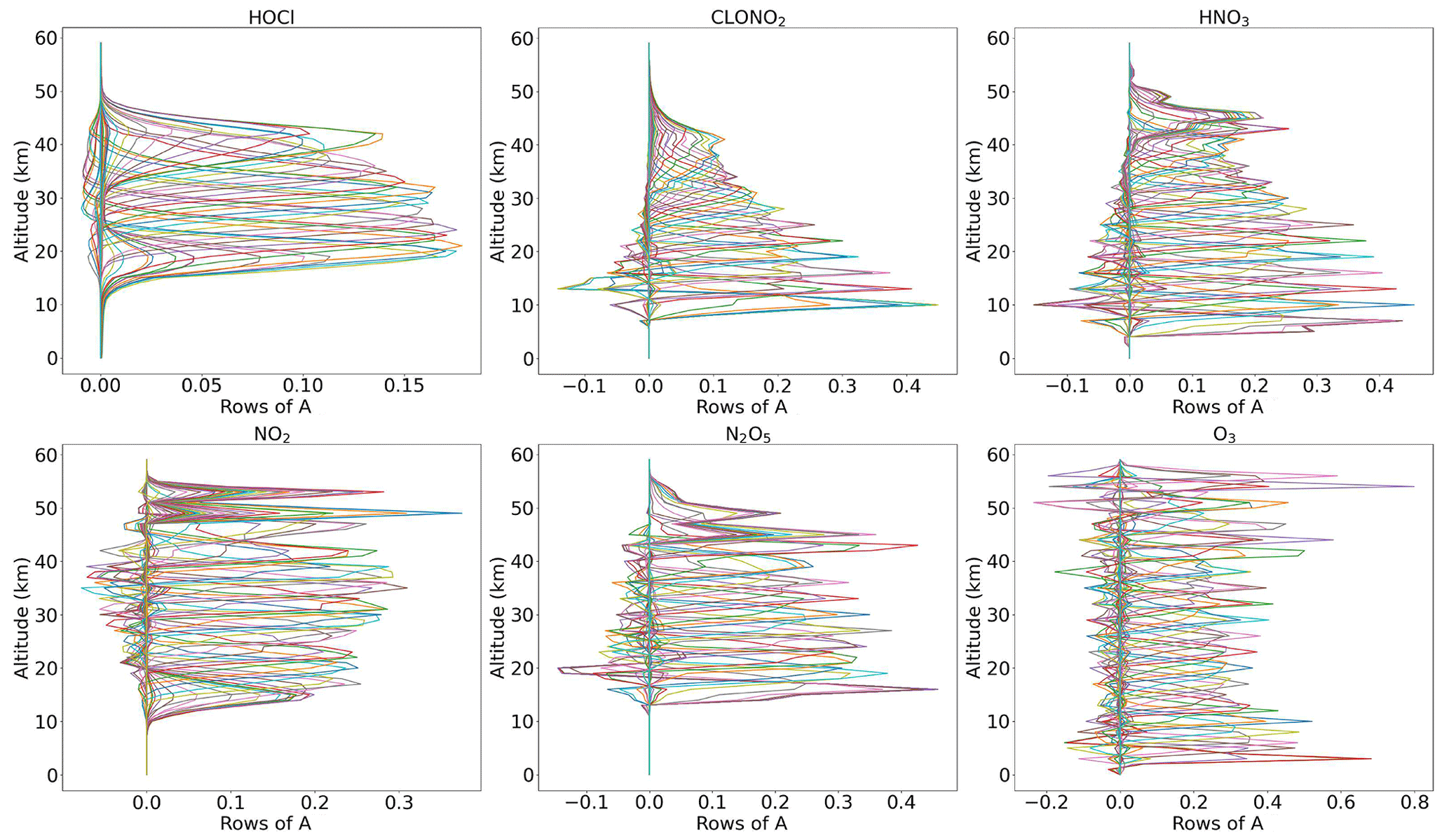
Figure 3 Example of rows of averaging kernels (A) for typical MIPAS HOCl, ClONO₂, HNO₃, NO₂, N₂O₅, and O₃ at a latitude of 67.5^∘ N on 27 October 2003 at 00:00 UT.

3 Comparison of ExoTIC simulations to MIPAS observations for the Halloween SPE 2003

In this section, a comparison study between the ExoTIC model results and MIPAS observations has been carried out for the chlorine species of HOCl, ClONO₂, ozone, and odd oxides of nitrogen (NO_y) for the Halloween SPE 2003. The comparison is done for the model simulations with different settings of ion chemistry, i.e. calculating the photo-chemical equilibrium of O(¹D) and switching off the uptake of chlorine ions and parameterized NO_x and HO_x. The model simulations are performed for a high latitude of 67.5^∘ N, and the MIPAS data are taken for the polar cap region, averaged over geographic latitudes such that MIPAS data are inside the vortex, vortex core, or vortex edge depending on the tracer properties. The model data are sampled in the MIPAS altitude grid as well. The day and night for the MIPAS data are sorted according to the solar zenith angle (sza) (day ≤ 90^∘; night > 98^∘). The solar zenith angles for the 1D model were chosen such that, for each day, this is the mean solar zenith angle for the MIPAS data plus or minus the standard error of the mean (SEM), with N being the number of data points for each day.

$$\begin{array}{}\text{(2)}& \mathrm{SEM}={\displaystyle \frac{\mathrm{standard}\mathrm{deviation}}{\sqrt{N}}}\end{array}$$

Since ExoTIC does not have diffusion or horizontal and vertical transport, the comparison can only be done for a short period of time. The model results are compared with the MIPAS observations for a total of 9 d from 26 October to 3 November 2003. Due to different vertical resolutions between the model and MIPAS observations, averaging kernels were applied. The averaging kernels were applied after sampling the model data in the MIPAS altitude grid. Now, ExoTIC being a 1D column model does not produce the output at the same geolocations as MIPAS, and hence the application of the MIPAS averaging kernels was based on the temperature criteria. The following procedure was applied for the convolution.

1. The model profiles were selected, one at a time, from the entire time series.

2. All the profiles from MIPAS within 57.5 and 77.5^∘ N latitude and ±6 h of the model profile's time were selected.

3. For this obtained MIPAS sample of temperature profiles, the root mean square value was calculated with the model's temperature profile, which is fixed for the entire time series.

4. The geolocation for which the root mean square value of the temperature difference profile was minimal was selected, and the averaging kernels for this geolocation were applied to the trace gas profiles from the model.

Using this procedure, we have obtained model profiles that were adjusted to the vertical resolution of MIPAS. The data were then averaged daily and the absolute or relative differences with respect to a day before the event, i.e. 26 October 2003 (day 299), was calculated.

3.1 Estimation of the polar vortex edge

There are different methods of estimating the vortex edge, and one of the methods widely used is to use CO as a tracer of vortex air. Due to its strong vertical gradient and longevity in the polar winter vortex, carbon monoxide is commonly used as a tracer of vortex air originating from the upper mesosphere and lower thermosphere. Hence it can be used to estimate the vortex edge. Here, we have used a CO vmr threshold (discriminating mesospheric air from the background) as a vortex criterion. We need an altitude-independent criterion (as we need to differentiate entire profiles), and our short time period (a few days) allows for a time-independent definition. A chemical vortex definition (via CO) is also widely used in the mesosphere (Harvey et al., 2015). For the chemical species and the SPE responses discussed here, the relevant altitude range is more in the stratosphere. In the stratosphere, the vortex might be considerably smaller and is commonly determined from the potential vorticity. Here, we use the tracer gradient instead to be consistent with the MIPAS observations that we use for comparison. Figure 4 shows volume-mixing ratios of CO versus latitude in the Northern Hemisphere for different longitude bins of size 20 (shown by different colours) and averaged over latitude bins of size 5 from 27 October (day 300) to 3 November 2003 (day 307) separated by daytime and nighttime. Choosing a threshold of 0.5 ppm of CO, the polar vortex boundary can be determined from the corresponding x axis, where an increase in the volume-mixing ratios starts to occur. An increase is observed starting at a latitude of approximately 55^∘ N for the different days. The estimation of the polar vortex boundary helps to choose the MIPAS sampling of the zonal averages for a better inter-comparison. One can also check the vortex boundary by looking at CH₄ zonal means, e.g. Fig. 9 of Funke et al. (2011). From that figure, and as also discussed in Funke et al. (2011), the boundary is around 60^∘ N, which also works well for the stratosphere. We chose the latitude 57^∘ N as where the vortex begins and defined the latitude bands 57–77^∘ N as “the edge region of the vortex” and the high-latitude bands 70–90^∘ N as “deep in the vortex”.

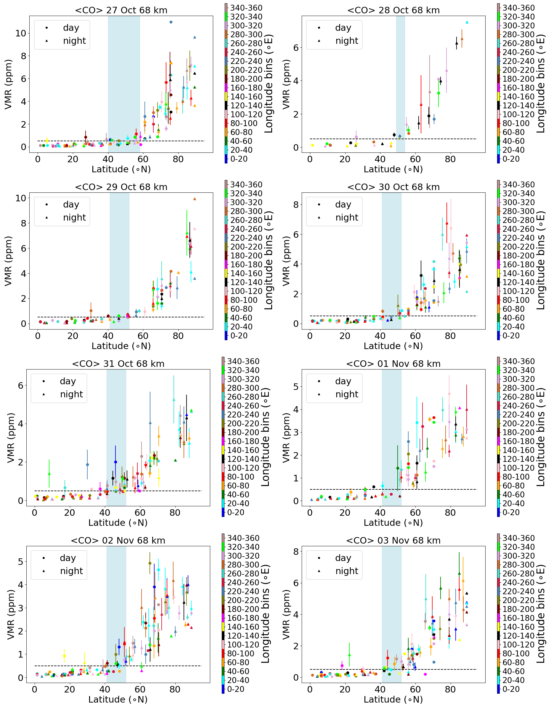
Figure 4 MIPAS daily averaged CO (ppm) as a function of latitude (^∘ N) for longitude bins of size 20 and averaged over latitude bins of size 5 for 27 October–3 November 2003 (day and night) at 68 km altitude. Colours mark the longitude bins from 0–20 to 340–360^∘ E running from blue to rosy brown. The error bars mark the standard error of the mean. The light-blue-shaded region marks the latitude range of the vortex edge and the dashed horizontal line is the CO threshold of 0.5 ppm.

3.2 HOCl change

A comparison of ENVISAT MIPAS V5 HOCl measurements (von Clarmann et al., 2006) for the polar Northern Hemisphere (57–77^∘ N) and ExoTIC computations with different settings of HOCl simulation is presented in Figs. 5 and 6 for daytime and nighttime respectively. The model data are read out in the solar zenith angle range of MIPAS daytime and nighttime observations. The values in both Figs. 5 and 6 start on 26 October 2003 (day 299). MIPAS observations for HOCl showed enhancements with peak values of 0.2 ppb for daytime and 0.24 ppb for nighttime on 29 October. The model results with full ion chemistry also overestimated the observed enhancements for nighttime by a factor of 4 (around 1.25 ppb) and for daytime by a factor of 3 (around 0.65 ppb) produced at an altitude of 35–40 km. HOCl enhancements below 30 km were also observed for both daytime and nighttime with full ion chemistry, and a peak producing 0.12 ppb was observed in the mesosphere during nighttime. Sensitivity studies were performed by setting O(¹D) to photo-chemical equilibrium, which showed a decrease in the enhancements from 1.25 to 0.55 ppb during nighttime and from 0.65 to 0.08 ppb during daytime produced by the model (also at 35–40 km during the event). The higher mixing ratios of HOCl below 30 km for both daytime and nighttime also disappeared with this setting. Switching off the chlorine ion chemistry led to the removal of 0.2 ppb HOCl observed in the mesosphere during nighttime. Similar behaviour was also observed for the parameterized NO_x and HO_x model. However, much lower values were observed during daytime for the model, setting O(¹D) to photo-chemical equilibrium without chlorine ion chemistry and parameterized NO_x and HO_x compared to MIPAS observations. Reaction rate constants and photo-chemical data in general follow the JPL-2006 recommendations from Sander et al. (2006).

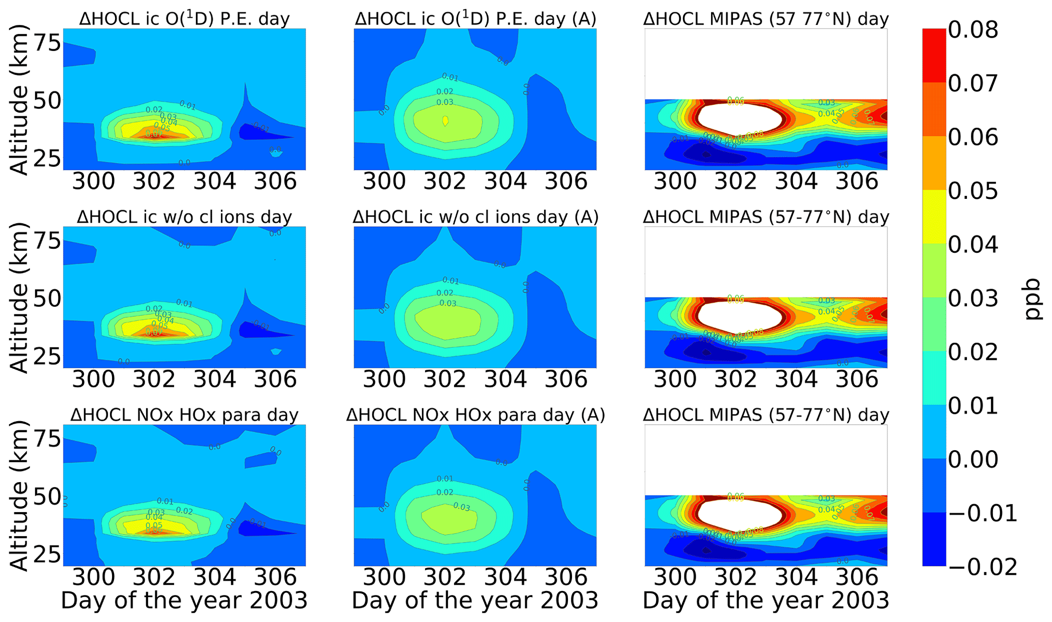
Figure 5 Absolute differences of daily averaged data for HOCl with respect to a day before the event, i.e. 26 October 2003. The starting point is 26 October 2003 for the three different model settings (sensitivity tests): (row-wise) ion chemistry with O(¹D) in photo-chemical equilibrium, switching off chlorine ion chemistry and parameterized NO_x and HO_x); (column-wise) without an averaging kernel (A) and with an averaging kernel (A) applied and MIPAS observations averaged over 57–77^∘ N for daytime (sza ≤ 90^∘). For daytime, the white region below 50 km is the MIPAS peak (0.2 ppb) and the colour bar is adjusted to the lower mixing ratios predicted by the model (first plot). The white region above 50 km for the MIPAS observations represents meaningless data where the values of averaging-kernel (A) diagonal elements are close to zero (<0.03), which indicates no sensitivity to the retrieved parameter at the corresponding altitude. Colour-bar interval: (−0.02, −0.01, 0.00, 0.01, 0.02, 0.03, 0.04, 0.05, 0.06, 0.07, 0.08).

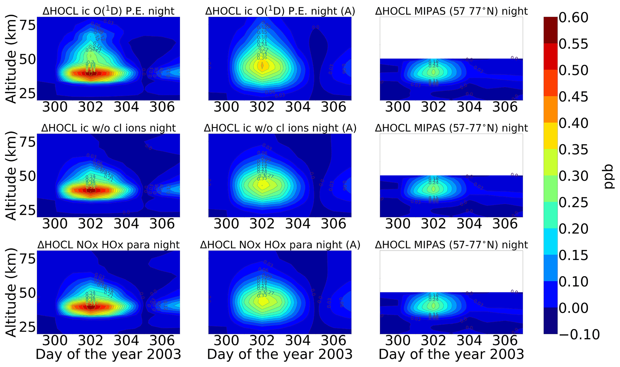
Figure 6 Same as Fig. 5 but for nighttime (sza > 98^∘). Colour-bar interval: (−0.10, 0.00, 0.10, 0.15, 0.20, 0.25, 0.30, 0.35, 0.40, 0.45, 0.50, 0.55, 0.60).

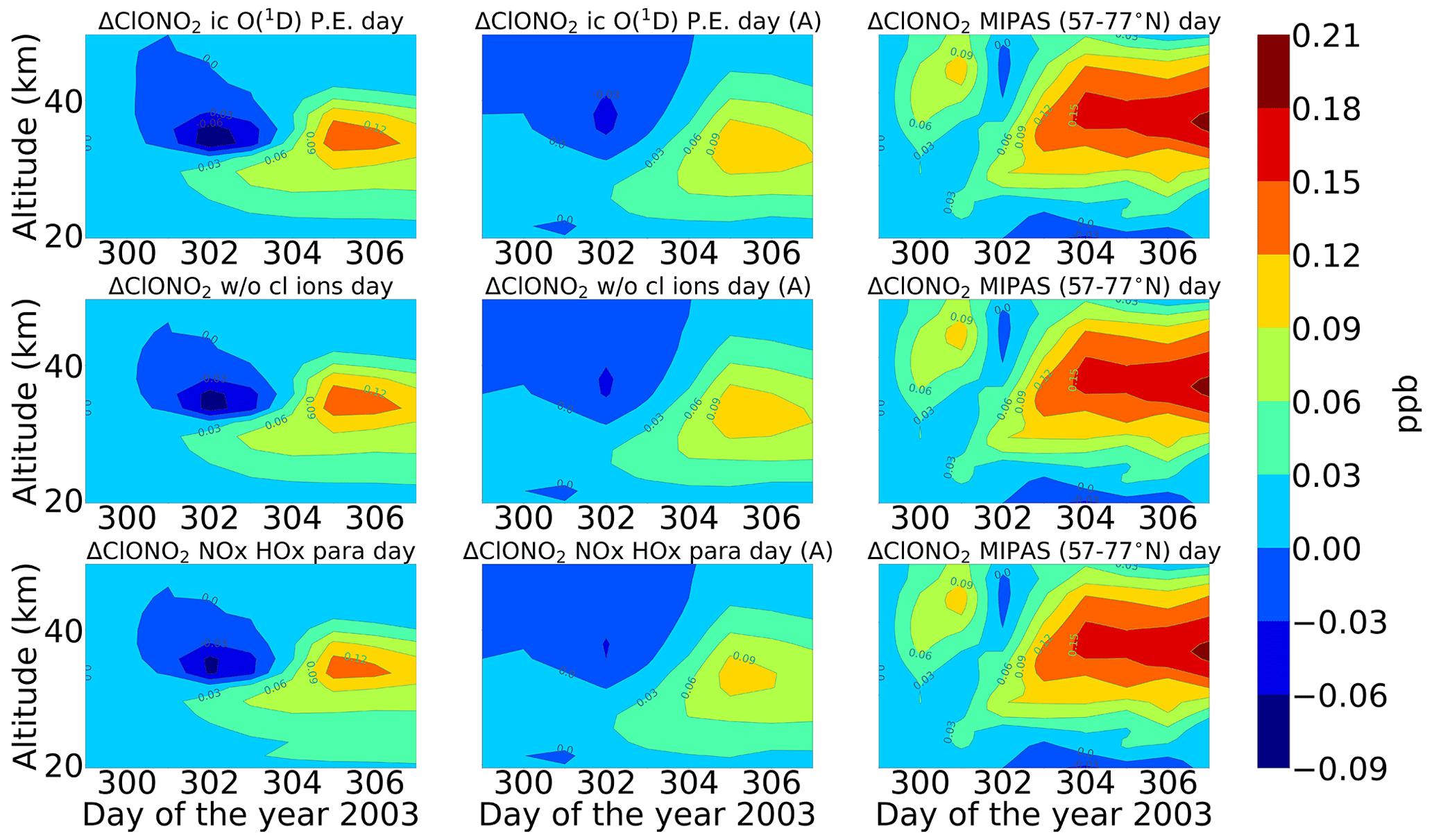
Figure 7 Same as Fig. 5 but for ClONO₂. Colour-bar interval: (−0.09, −0.06, −0.03, 0.00, 0.03, 0.06, 0.09, 0.12, 0.15, 0.18, 0.21).

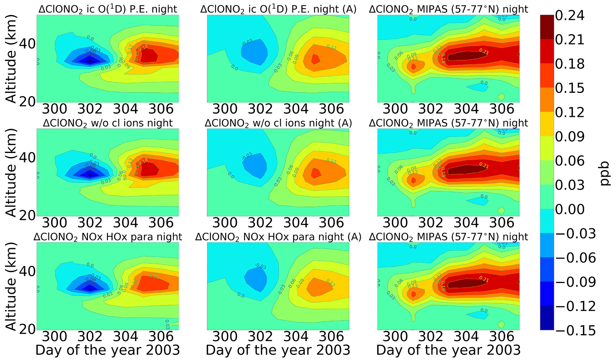
Figure 8 Same as Fig. 6 but for ClONO₂. Colour-bar interval: (−0.15, −0.12, −0.09, −0.06, −0.03, 0.00, 0.03, 0.06, 0.09, 0.12, 0.15, 0.18, 0.21, 0.24).

After the application of averaging kernels, the higher mixing ratios produced by the model were smeared out over altitudes and reduced in their peak value. For daytime, the peak value of the full ion chemistry model decreased from 0.65 to 0.4 ppb. For the sensitivity studies with O(¹D) in photo-chemical equilibrium and without chlorine ion chemistry and parameterized NO_x and HO_x, the peak value of 0.08 ppb decreased to 0.03 ppb. This peak value occurs due to the increased availability of chlorine atoms due to the catalytic ozone destruction cycle. The HOCl concentration reaches a peak around 35 km during daytime because this altitude represents the optimal conditions for the ClO–HOCl catalytic cycle (Reactions R19–R22) to occur. For nighttime, the full ion chemistry peak value of 1.25 ppb went down to 0.84 ppb after applying the MIPAS averaging kernels. Setting O(¹D) to photo-chemical equilibrium decreased the peak value from 0.55 to 0.36 ppb, which is in better agreement with the MIPAS observations. For the model without chlorine ion chemistry and parameterized NO_x and HO_x, the enhancements of 0.58 ppb went down to 0.33 ppb, which also agrees quite well with the “MIPAS observations”. Jackman et al. (2008) compared results from WACCM3 with MIPAS observations, applied MIPAS averaging kernels for the Halloween SPE 2003, and found the HOCl peak at an altitude of 48 km on 29 October; the MIPAS averaging kernels moved the HOCl peak at altitude 48 km down to 40 km. ExoTIC however produced the peak around 35–40 km for both daytime and nighttime and for all the test cases. This is actually quite in agreement with the MIPAS observations, and the application of the averaging kernels also did not shift the peak in terms of altitude. This difference in the peak altitude between the results from Jackman et al. (2008) and ExoTIC might be due to the fact that WACCM3 has fully interactive dynamics, radiation, chemistry, and other parameterizations, whereas ExoTIC includes only the chemistry. Damiani et al. (2012) considered the SPE of January 2005, where they observed a 0.2 ppb increase in HOCl during the event in the polar cap region, also using the WACCM model that agreed quite well with Microwave Limb Sounder (MLS) observations. Enhancements of HOCl result from enhanced HO_x constituents. In the middle stratosphere, this is mainly accelerated by odd hydrogen chemistry (via Reaction R19). The morphology of the HOCl distribution and its temporal variation are a combined effect of the photolysis, temperature, and availability of ClO, HO₂, and OH, which in themselves show a pronounced diurnal variation.

Figure 9 Same as Fig. 5 but for NO_y species. Colour-bar interval: ($-{\mathrm{10}}^{-\mathrm{1}}$, −10⁰, 0, 10⁰, 10¹, 2×10¹, 3×10¹, 4×10¹, 6×10¹, 10²).

3.3 ClONO₂ change

Figures 7 and 8 show the daily averaged absolute differences for ENVISAT MIPAS V5 (Höpfner et al., 2007) and modelled chlorine nitrate with respect to 26 October 2003 for daytime and nighttime. The zonal average for ClONO₂ observations was also taken over a latitude range of 57–77^∘ N, the edge region of the polar vortex. Continuous enhancements of ClONO₂ are observed for the full ion chemistry model, with peak values of 0.96 and 1.15 ppb approximately 2 d after the event for daytime and nighttime respectively starting from the onset of the event on 28 October. The peak was observed around 25 km. In the case of the model with ion chemistry but O(¹D) set to photo-chemical equilibrium, a peak value of around 0.18 ppb was observed for both daytime and nighttime, which agreed much better with the MIPAS observations. Similar results were also observed for the sensitivity study without chlorine ion chemistry and the parameterized NO_x and HO_x model. The increase was also seen approximately 2 d after the event in the altitude range 35–40 km. After the application of averaging kernels, the peak value for the full ion chemistry during daytime and nighttime decreased to 0.66 and 0.78 ppb respectively. For the rest, the peak value decreased from 0.12 to 0.09 ppb for daytime and from 0.18 to 0.12 ppb for nighttime. Jackman et al. (2008) observed ClONO₂ maximum enhancements of 0.3–0.4 ppb with a peak production at a higher altitude of 40–45 km with WACCM3. The peak was however produced several days later than MIPAS. The application of MIPAS averaging kernels moved the peak down to 40 km, and the predicted peak increases are reduced substantially to about 0.2 ppbv (about a factor of 2 less than MIPAS observations).

The enhanced ClONO₂ production happens due to SPE-produced NO_x via Reaction (R32). ClONO₂ is removed mainly by photolysis in the sunlit atmosphere and, to a lesser extent, by reaction with atomic oxygen. Due to its pressure dependence, ClONO₂ formation by Reaction (R32) is more effective at lower altitudes (Funke et al., 2011). The zonal averages of MIPAS observations were tested for latitude bands 57–77^∘ N, i.e. in the edge region of the polar vortex, and 70–90^∘ N, deep in the polar vortex. The sample of 57–77^∘ N works better for the inter-comparison of ClONO₂ compared to 70–90^∘ N. In the case where the sample is taken deep in the vortex, the model seems to fairly underestimate the peak values. This can be explained by Reaction (R32), where formation of ClO needs sunlight, which is again more available in the edge region of the polar vortex. However, ClONO₂ can also photolyse in the presence of sunlight and, due to this, there is a balance between the two processes and ClONO₂ can form in the edge region. This can be transported deep into the vortex and conserved there at high latitudes. This cannot however be reproduced by the 1D model because it is fixed at a certain location and has no transport.

Figure 10 Same as Fig. 6 but for NO_y species. Colour-bar interval: ($-{\mathrm{10}}^{-\mathrm{1}}$, −10⁰, 0, 10⁰, 10¹, 2×10¹, 3×10¹, 4×10¹, 6×10¹, 10²).

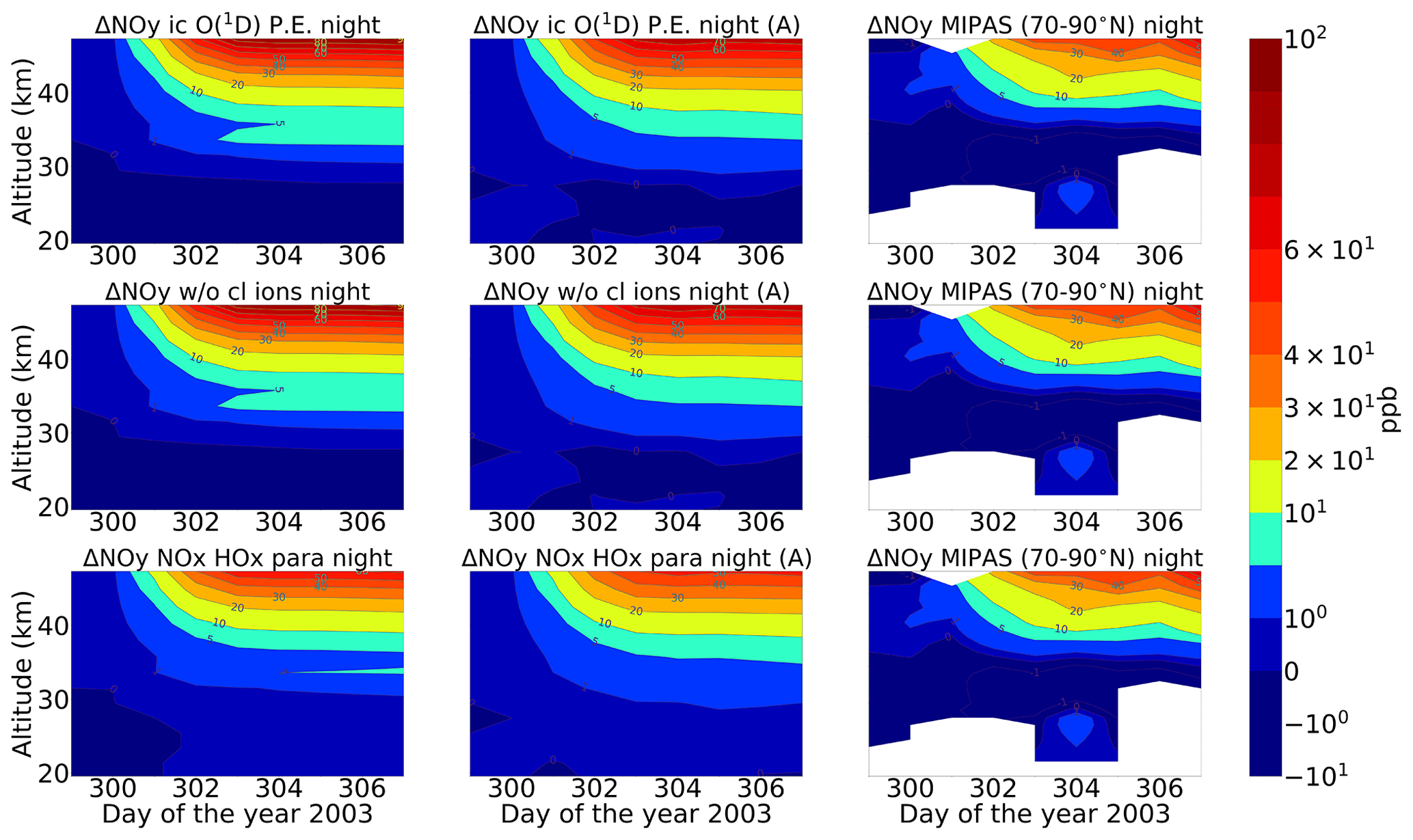
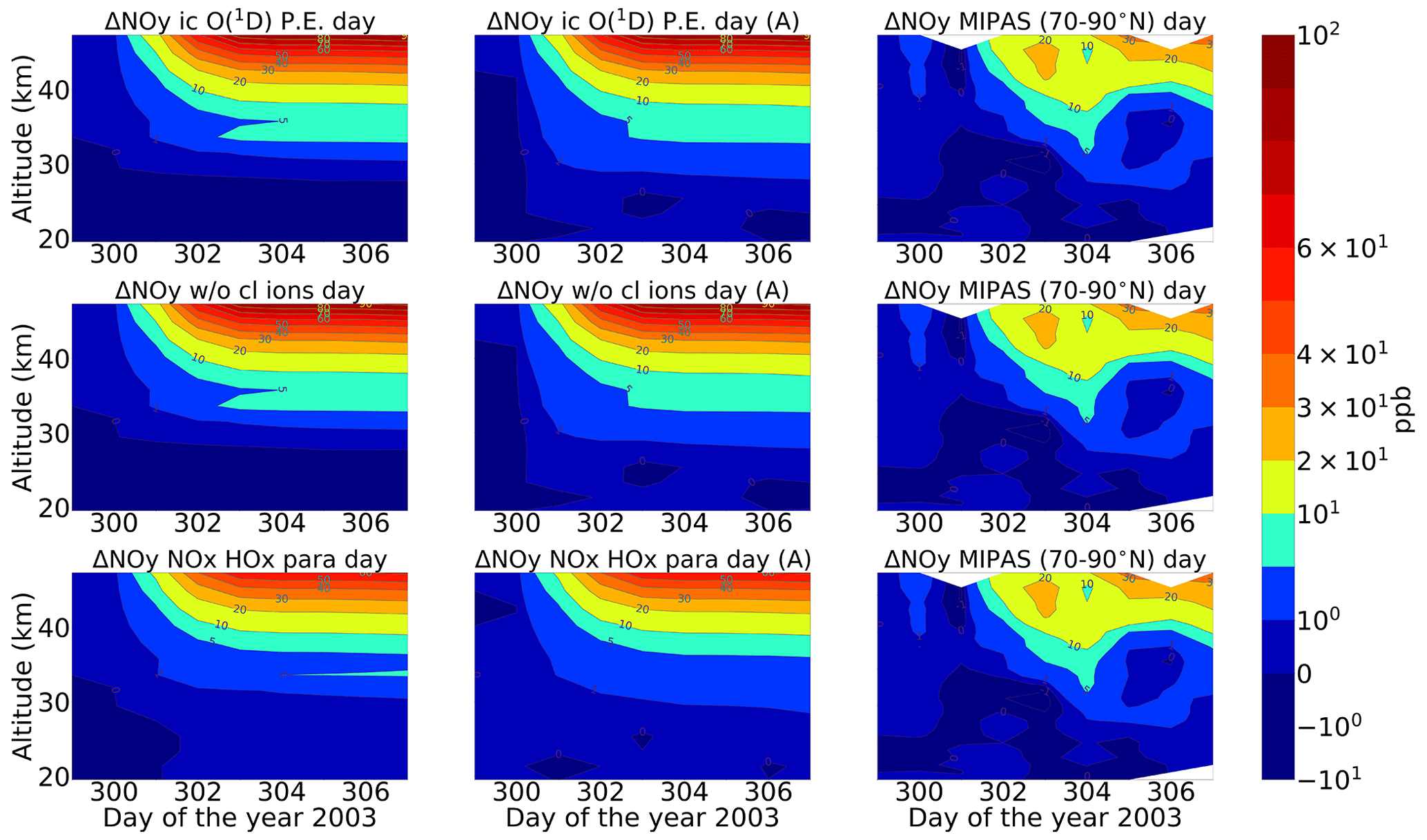
3.4 Odd oxides of nitrogen (NO_y)

An important impact of proton precipitation in the middle atmosphere is the formation of NO_x, which happens by the dissociation of molecular nitrogen by ionization and subsequent recombination with oxygen. In order to assess the agreement of the ENVISAT MIPAS V5 (Funke et al., 2005) and modelled SPE-related odd nitrogen enhancements, total NO_y (NO + NO₂ + HNO₃ + 2N₂O₅ + ClONO₂) is compared. The observed and modelled NO_y enhancements with respect to 26 October are shown in Figs. 9 and 10 for daytime and nighttime conditions respectively. Averaging kernels are also applied to the model profiles for the different NO_y species for the different model settings and are then added, except for NO. In the case of MIPAS NO and NO₂ data, there is a complication, which is that, instead of mixing ratios, the logarithms of the mixing ratios are retrieved. Also, the averaging kernels refer to the logarithms of the mixing ratios. The application of MIPAS averaging kernels to a better-resolved profile on the basis of the coarse-grid averaging kernel A of the logarithm of the mixing ratio is then (Stiller et al., 2012)

$$\begin{array}{}\text{(3)}& {\mathit{x}}_{\mathrm{new}}=\exp \left(\mathbf{A}\log \left({\mathit{x}}_{\mathrm{orig}}\right)+(\mathbf{I}-\mathbf{A})\log \left({\mathit{x}}_{\mathrm{a}}\right)\right).\end{array}$$

There is a general issue with logarithmic retrievals, because regularization is self-adaptive and depends on the actual state of the atmosphere. For an SPE response, if the NO peaks around 50–60 km and if there is a better sensitivity at this altitude, the Jacobian and the averaging kernels scale with the volume-mixing ratio. For NO₂, however, the logarithmic averaging kernels behave well and are not dependent on the actual conditions (for a deeper discussion of the problem of time- and state-dependent averaging kernels, see von Clarmann et al., 2020). Due to this complication, for the total NO_y in the second columns of Figs. 9 and 10 for both daytime and nighttime, NO is added without the application of the averaging kernels as compared to the rest of the species.

The magnitude of NO_y enhancements is found to be larger for the ExoTIC model with ion chemistry settings compared to the MIPAS observations for both daytime and nighttime. However, the SPE-induced NO_y layer is reproduced well in terms of vertical distribution. The MIPAS observations showed productions of 30–40 ppb in the upper stratosphere during nighttime and 20–30 ppb during daytime. The MIPAS observations show much higher dynamics than ExoTIC for both daytime and nighttime. The nighttime values show stronger dynamics with decreased ionization rates on days 305–306 and, connected to this, less ΔNO_y reaches a constant state after the maximum of the first SPE on day 303. This could be an indication that some of the NO_y recombination speeds are faster than expected. The results are shown up to 50 km since above 50 km NO is the largest contributor (Funke et al., 2011) and averaging kernels are not applied to NO. Another reason is that large uncertainties in small vmr values of ClONO₂ (Höpfner et al., 2007) will spoil the NO_y sum and its uncertainty. The nighttime results compare better with the observations, especially for the parameterized NO_x and HO_x model. For daytime, the model with and without an averaging kernel (A) did not make too much of a difference because NO was added without an averaging kernel (A) and was abundant during daytime.

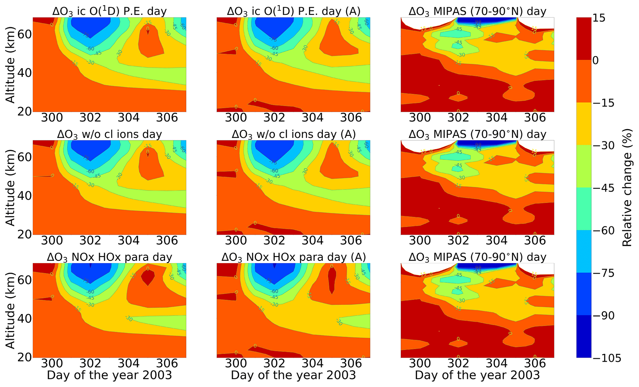
Figure 11 Relative difference of ozone with respect to 26 October. The rest is the same as Fig. 5. Colour-bar interval: (−105, −90, −75, −60, −45, −30, −15, 0, 15).

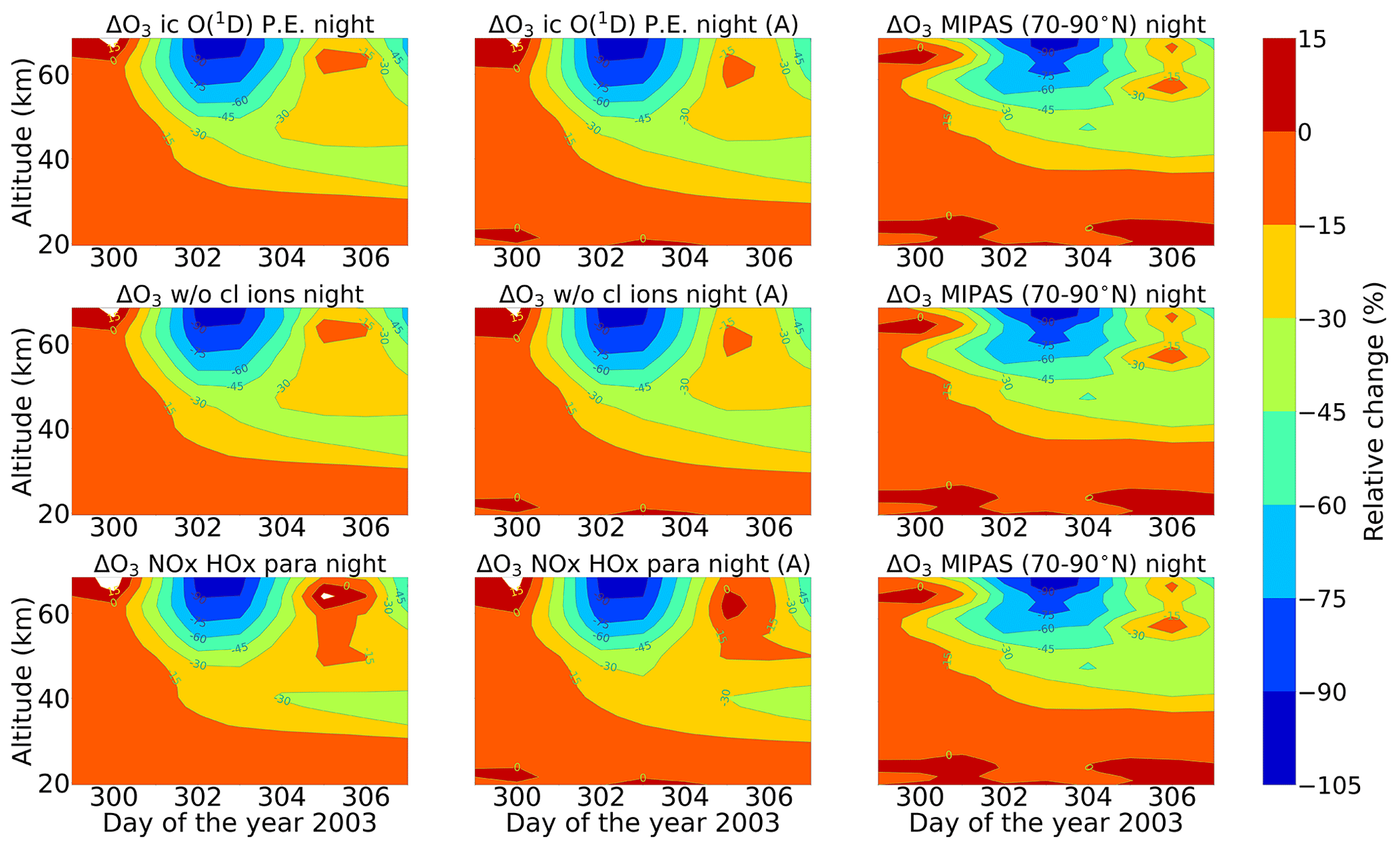
Figure 12 Same as Fig. 11 but for nighttime. Colour-bar interval: (−105, −90, −75, −60, −45, −30, −15, 0, 15).

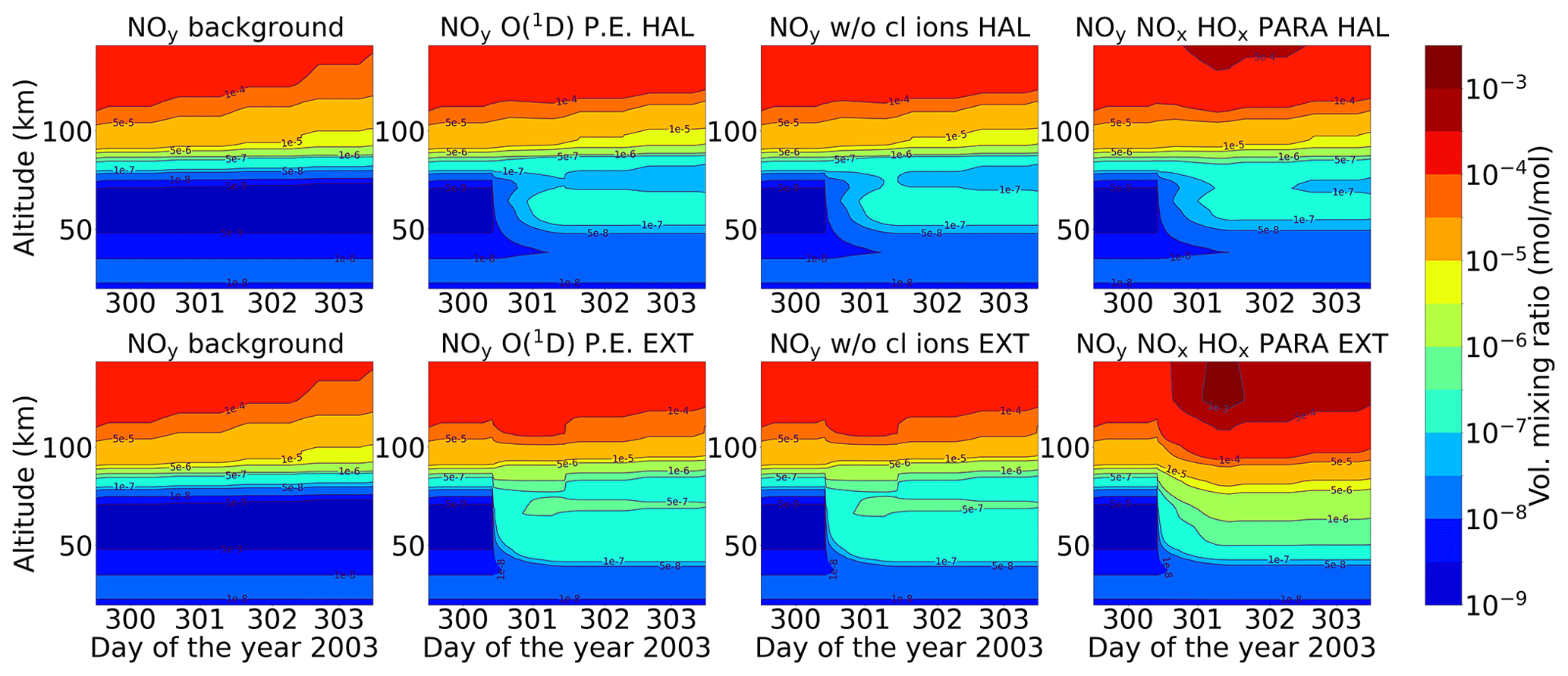
Figure 13 Comparison of the Halloween SPE and the extreme scenario (row-wise) for $\stackrel{\mathrm{̃}}{{\mathrm{NO}}_y}$: reference run (background atmosphere) and full ion chemistry with O(¹D) set to photo-chemical equilibrium, without chlorine ions and the parameterized NO_x and HO_x model (column-wise) for a high latitude of 67.5^∘ N.

3.5 Ozone

Energetic particles in the polar atmosphere enhance the production of NO_x and HO_x in the winter stratosphere and mesosphere. Both NO_x and HO_x are powerful ozone destroyers. An important aspect in the evaluation of the ability of models is the reproduction of the observed ozone destruction caused by the catalytic cycles of NO_x and HO_x during SPE-induced chemical composition changes. As inferred from observations, stratospheric ozone decreases due to the indirect effect of EPP by about 10 %–15 % as observed by satellite instruments (Meraner and Schmidt, 2018). López-Puertas et al. (2005) found HO_x-related mesospheric ozone losses of up to 70 % and NO_x-related stratospheric losses of around 30 % during the Halloween SPE.

Figures 11 and 12 show ENVISAT MIPAS V5 (Glatthor et al., 2006) and the modelled temporal evolution of the relative ozone changes with respect to 26 October, averaged over 70–90^∘ N for daytime and nighttime respectively. For ozone, the long-term history of air parcels is more important, as air parcels that are ozone-depleted are dispersed into the mid-latitudes if they are in the edge region of the vortex. So, a sample deeper in the vortex for ozone is better, which is the reason we chose 70–90^∘ N here. A loss of 60 %–75 % is observed during the event itself in the mesosphere that is short-lived and that is related to the HO_x catalytic cycle (Reactions R6, R7, R9, and R10, Funke et al., 2011; Bates and Nicolet, 1950). The ozone recovers after the event, since HO_x is short-lived. A second peak is observed on 3 November that is related to a weaker coronal mass ejection event. A NO_x-related loss of 15 % is observed in the stratosphere, lasts longer, and is also related to the polar winter atmosphere (Reactions R12 and R13). The full ion chemistry shows an ongoing loss of 45 % starting from the event day, and the sensitivity study with O(¹D) in photo-chemical equilibrium confirmed that this loss is due to reactions like Reactions (R40) and (R37), which produce OH and Cl, contributing further to ozone loss. The agreement between the observations and the model results, for nighttime, for the three model results except for the full ion chemistry is excellent in the mesosphere, indicating the good ability of the model to reproduce HO_x-related ozone loss for SPEs. However, the ozone loss shifted to lower altitudes for both daytime and nighttime in all the model settings as compared to MIPAS observations. This could be explained as a result of the AISstorm ionization rates, which were used in the model and could be different to what MIPAS might have experienced during the SPE. Here, AISstorm uses proton fluxes from GOES 10, and the ionization rates should be a lower estimate. The SPE ionization happens in the denser atmosphere, and therefore the conversion from particle fluxes into ionization should be more or less precise in terms of total ionization and altitude. The main uncertainty in SPE ionization in AISstorm is the size of the area that is affected by high-energy particle precipitation. This cannot be derived from these channels but is taken from a lower-energy channel on another satellite, and thus it might be an underestimate of the polar cap size. However, if this is important for the spatial average 70–90^∘ N, we should see an underestimation of the ionization (and NO_y) as well, which does not seem to be the case (and which is unlikely anyway as the equatorward boundary should be at about 60^∘ N).

4 Comparison of the Halloween storm and the extreme solar event of AD 775

In this section, a comparison study between the Halloween storm of 2003 and the extreme event of AD 775 is presented. The model simulations are performed at a latitude of 67.5^∘ N and begin at noon on 27 October (day 300). The ionization rate profiles are obtained from AISstorm for both the events and are inputted from noon on 28 October to noon on 29 October. Since the studies were performed without horizontal and vertical transport, the results shown here are restricted to a short time period. The results are shown for the model simulations for the settings that compared well with MIPAS observations.

Figure 14 Same as Fig. 13 but for odd hydrogen species (HO_x).

4.1 $\stackrel{\mathrm{̃}}{{\mathrm{NO}}_y}$ and HO_x

Figure 13 shows the formation of $\stackrel{\mathrm{̃}}{{\mathrm{NO}}_y}$ during the Halloween SPE and the extreme scenario with different settings of the ion chemistry. $\stackrel{\mathrm{̃}}{{\mathrm{NO}}_y}$ consists of species of odd nitrogen as shown in Eq. (4):

$$\begin{array}{}\text{(4)}& \stackrel{\mathrm{̃}}{{\mathrm{NO}}_y}=\mathrm{NO}+{\mathrm{NO}}_{\mathrm{2}}+\mathrm{N}+{\mathrm{HNO}}_{\mathrm{3}}+\mathrm{2}{\mathrm{N}}_{\mathrm{2}}{\mathrm{O}}_{\mathrm{5}}+{\mathrm{NO}}_{\mathrm{3}}+{\mathrm{ClONO}}_{\mathrm{2}}.\end{array}$$

After the onset of the event, $\stackrel{\mathrm{̃}}{{\mathrm{NO}}_y}$ starts accumulating over time in the stratosphere and lower mesosphere. For the extreme scenario, the vmr of $\stackrel{\mathrm{̃}}{{\mathrm{NO}}_y}$ is about 1 order of magnitude larger compared to the Halloween SPE in the upper stratosphere and lower mesosphere. For example, the amount of $\stackrel{\mathrm{̃}}{{\mathrm{NO}}_y}$ at 60 km is found to be 50 ppb for the Halloween event compared to 500 ppb for the extreme event. Additionally, for the extreme event, $\stackrel{\mathrm{̃}}{{\mathrm{NO}}_y}$ is seen to be formed even in the lower stratosphere (below 30 km). This is because of the high values of ionization rates that reached further down in altitude in this case. A small difference was observed between the sensitivity study without the chlorine ion chemistry and the model setting of ion chemistry with O(¹D) in photo-chemical equilibrium around 75 km. The full ion chemistry and the ion chemistry setting O(¹D) to photo-chemical equilibrium did not show much of a difference. For the parameterized model, $\stackrel{\mathrm{̃}}{{\mathrm{NO}}_y}$ enhancements are observed in the mesosphere and lower thermosphere, with higher values seen for the extreme scenario compared to the Halloween event. Since only N, NO, and NO₂ are present for the parameterized NO_x, the impact of the scavenging reaction, Reaction (R2), is stronger, and the partitioning between N and NO is different compared to the ion chemistry, which also contains other $\stackrel{\mathrm{̃}}{{\mathrm{NO}}_y}$ species like HNO₃. Reaction (R2) drives the NO_x parameterization and makes the main difference with respect to the ion chemistry. In contrast to our results, which show the total NO_y that includes NO_x = N + NO, Andersson et al. (2016) showed that WACCM-D with the D-region ion chemistry predicts more NO_x in the mesosphere compared to WACCM with the standard parameterization of NO_x and HO_x production for the northern polar cap region (latitude > 60^∘ N during the SPE of January 2005). Kalakoski et al. (2020) also reported the same when considering SPEs using proton flux data from satellite-based GOES observations. They considered an event in which the peak proton flux exceeded 100 pfu (particle flux units), with pfu defined as the 5 min average flux in units of particles (cm⁻² s⁻¹ sr⁻¹) for protons with energy higher than 10 MeV. The rate of formation of NO_x = N + NO is indeed higher in the mesosphere when full ion chemistry is considered, but the partitioning between the formation of N and N(²D)−forming NO is also increasingly in favour of N, meaning that the rate of loss of NO is also faster in this altitude range when full ion chemistry is considered. This can lead to less NO, depending on the absolute rate of NO_x formation and the partitioning between N and NO in this formation. The HO_x parameterization does not make much of a difference for $\stackrel{\mathrm{̃}}{{\mathrm{NO}}_y}$.

Figure 15 Same as Fig. 13 but for HCl.

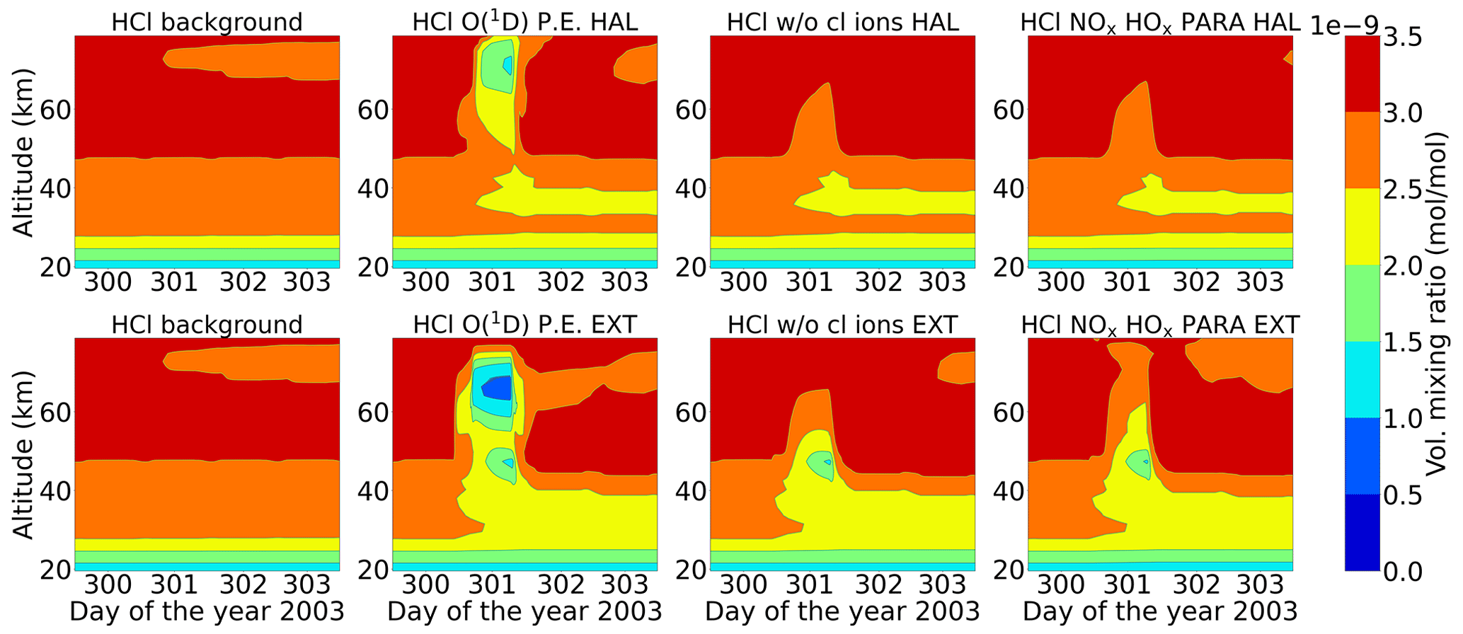
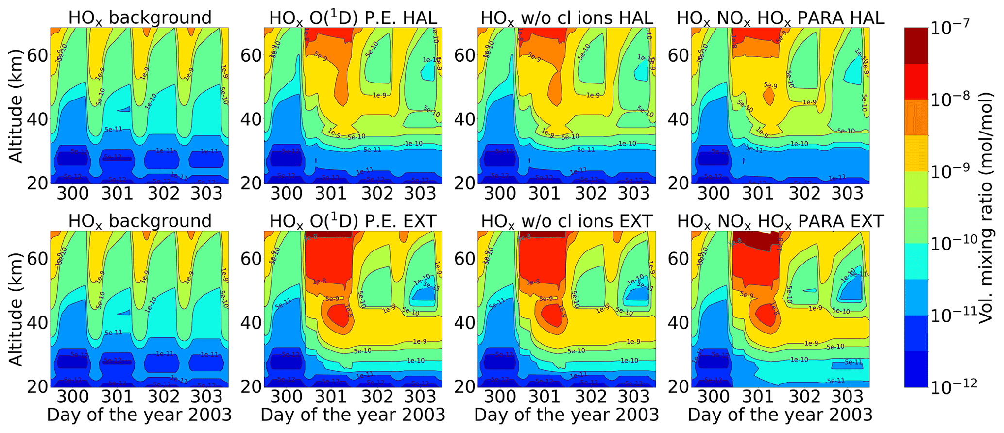
Figure 14 shows the temporal evolution of HO_x for the Halloween SPE and extreme scenario that consists of odd hydrogen species (Eq. 5).

$$\begin{array}{}\text{(5)}& {\mathrm{HO}}_x=\mathrm{H}+\mathrm{OH}+{\mathrm{HO}}_{\mathrm{2}}+\mathrm{2}{\mathrm{H}}_{\mathrm{2}}{\mathrm{O}}_{\mathrm{2}}\end{array}$$

HO_x was not shown for the MIPAS comparison due to the fact that H and OH are not provided by MIPAS. HO_x enhancements are seen during the event. For the Halloween SPE, HO_x enhancements of 0.1 ppm were observed in the mesosphere during the event, whereas for the extreme scenario, these enhancements were seen to penetrate deep down. However, after the event stops, the HO_x disappears at higher altitudes, since it is short-lived up there. However, at lower altitudes, around 25–40 km, HO_x enhancements of around 1 ppb were found to be continuous and more persistent, especially for the extreme scenario. The full ion chemistry shows HO_x enhancements below 30 km due to the presence of O(¹D), which can react with water vapour, hydrogen, and methane via Reactions (R37)–(R39). However, with O(¹D) set to photo-chemical equilibrium, the HO_x enhancements below 30 km disappeared for both events. The impact of chlorine ion chemistry is seen to be rather small. For the parameterized model, the recovery of HO_x after the event was found to be slower compared to the ion chemistry model. The high values of HO_x are balanced by the continuous destruction of water vapour, and when it is completely destroyed, the HO_x formation breaks down. So, the full parameterization with both NO_x and HO_x is different, but the water vapour is a limiting factor for both. The ion chemistry with more HO_x can also lead to a faster reaction between OH and NO₂ (Reaction R41), which can produce HNO₃ and contribute a difference to the recovery of HO_x.

$$\begin{array}{}\text{(R41)}& \mathrm{OH}+{\mathrm{NO}}_{\mathrm{2}}⟶{\mathrm{HNO}}_{\mathrm{3}}\end{array}$$

4.2 Chlorine species

Figure 15 shows the volume-mixing ratios of HCl for the two events. Loss of HCl, which can occur via transformation into reactive chlorine as it is taken up from the gas phase into negative ions, is seen during the event in both cases but is more pronounced for the extreme scenario. This occurred in both the stratosphere and mesosphere for full ion chemistry. Negative ions upon reaction with HCl can form Cl⁻ ions, which form large-cluster ions and thereby release Cl upon recombination (Sinnhuber et al., 2012).

$$\begin{array}{}\text{(R42)}& {\displaystyle }& {\displaystyle }\mathrm{HCl}+X^{-}⟶{\mathrm{Cl}}^{-}+\mathrm{H}X\text{(R43)}& {\displaystyle }& {\displaystyle }{\mathrm{Cl}}^{-}+Y⟶{\mathrm{Cl}}^{-}Y\end{array}$$

$$\begin{array}{}\text{(R44)}& {\mathrm{Cl}}^{-}\left(Y\right)+{\mathrm{Z}}^{+}⟶\mathrm{Cl}+Z+Y\end{array}$$

X = O, O₂, CO₃, OH, NO₂, and NO₃. Y = HCl, H₂O, and CO₂, and Z is positive ions (Kopp and Fritzenwallner, 1997). Cl⁻ and Cl⁻ cluster ions like Cl⁻(H₂O) can also release HCl via reaction with H (Kopp and Fritzenwallner, 1997). HCl can react with O(¹D) via Reaction (R40), resulting in an enhanced loss of HCl below 40 km, but this disappears when O(¹D) is set to photo-chemical equilibrium. At 40–50 km, ExoTIC with ion chemistry and O(¹D) set to photo-chemical equilibrium observed 5 %–15 % HCl loss for the Halloween SPE and 20 %–45 % HCl loss for the extreme event. From the sensitivity study without the chlorine ions, it is evident that the huge HCl loss of around 75 % observed in the mesosphere is due to the chlorine ion chemistry. The parameterized model underestimates the loss of HCl which was also found in the study by Winkler et al. (2009).

The primary neutral reaction that leads to the decrease in HCl below 50 km is a series of reactions involving HO_x species that are part of the catalytic ozone destruction cycle (Reactions R6 and R7). The decrease in ozone concentration has a secondary effect on the concentration of HCl. In the absence of an SPE, ozone plays a role in the conversion of ClO back to HCl. However, during an SPE, the enhanced ionization and subsequent formation of ions disrupt this ozone destruction and formation cycle. This leads to an increase in the concentration of ClO and a subsequent reduction in the concentration of HCl. The excess ClO can further participate in additional ozone depletion cycles, leading to a decline in ozone levels during the event. Andersson et al. (2016) reported daily averaged anomalies of HCl in both hemispheres for the latitudinal band 60–82.5^∘ N at altitudes between 40 and 52 km. They compared WACCM-D consisting of the D-region ion chemistry and WACCM consisting of the standard NO_x and HO_x parameterization with MLS observations. They found a rapid HCl decrease of about 2 %–6 % during the January 2005 SPE in both hemispheres. With WACCM-D, a loss of around 4 % was found compared to a loss of 3 % in the standard WACCM in the Northern Hemisphere. They also showed that WACCM-D showed better agreement with MLS observations.

Since $\stackrel{\mathrm{̃}}{{\mathrm{NO}}_y}$ and HO_x production is enhanced during SPEs, which is evident from Figs. 13 and 14, they can react with reactive chlorine species like ClO. ClO can react either with HO_x, producing short-term enhancement in HOCl (Reaction R19), or with NO_x, slowly producing ClONO₂ (Reaction R32). ClO is formed from the reactive Cl via Reaction (R21) by neutral gas-phase reactions of Cl with ozone in the altitude range 35–40 km.

Figure 16 Same as Fig. 15 but for ClO.

Figure 17 Same as Fig. 15 but for HOCl.

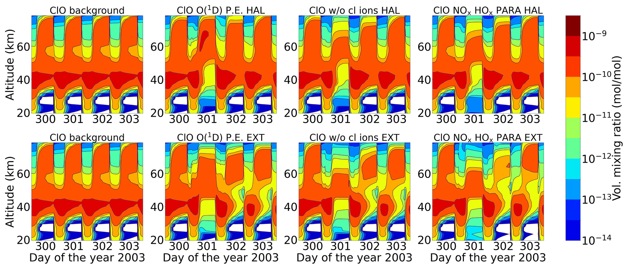
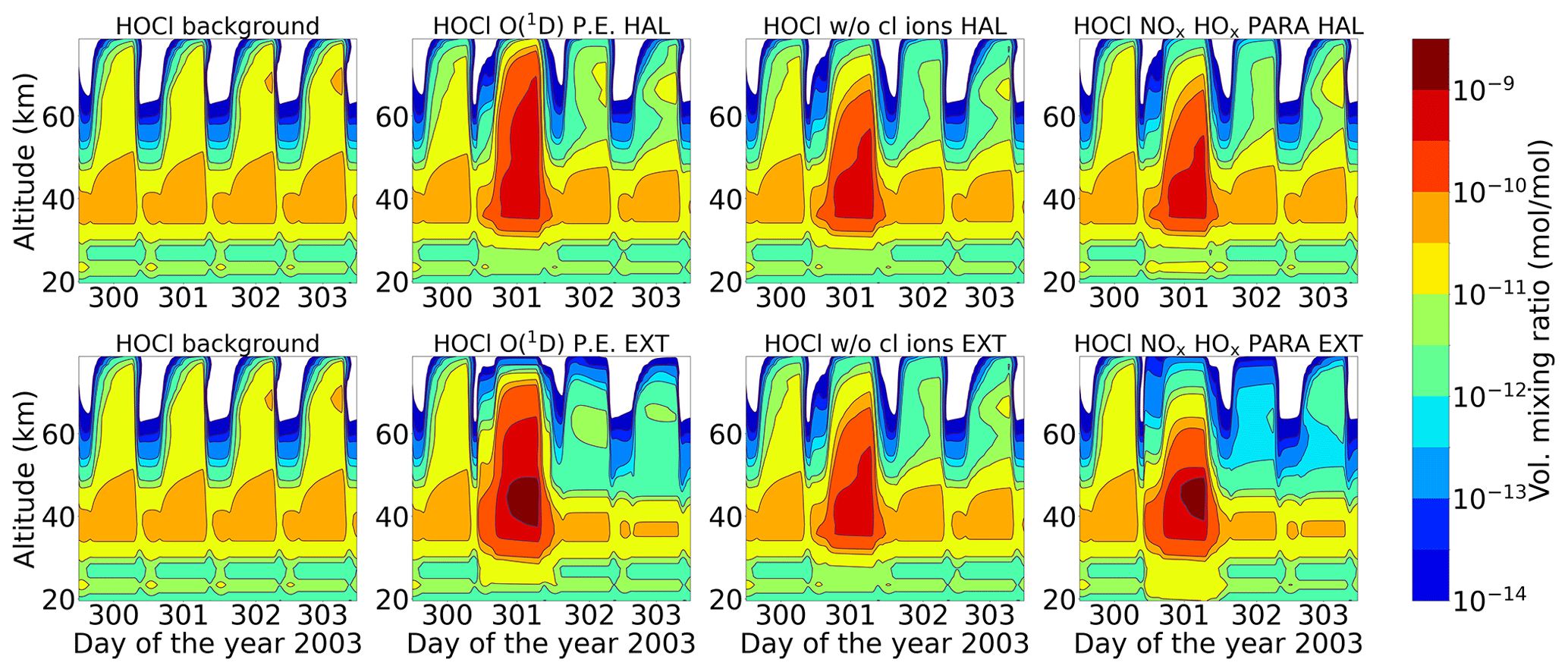
From Fig. 16, it can be seen that ClO decreases during the event for the same altitude range but recovers straight after the event stops. ClO can react with HO_x species during SPEs, particularly HO₂, to produce HOCl (Reaction R19), which is also a short-lived species. Therefore, a short-term enhancement of HOCl is seen during both events (Fig. 17), which was also observed by von Clarmann et al. (2005) for the Halloween SPE. However, for the extreme scenario, loss of ClO continues, especially around 30–40 km, even after the event stops. This is because of the excess NO_x available for the extreme event due to which Reaction (R32) can happen continuously, which is supplemented by an increase in ClONO₂ after the extreme event as seen in Fig. 18. Loss of HOCl seen after the extreme event is due to excess HO_x as well. HOCl can react with OH to form ClO (Reaction R24), and then ClO can react back with HO₂; this catalytic cycle thereby results in the loss of both species due to excess HO_x.

Figure 18 Same as Fig. 15 but for ClONO₂.

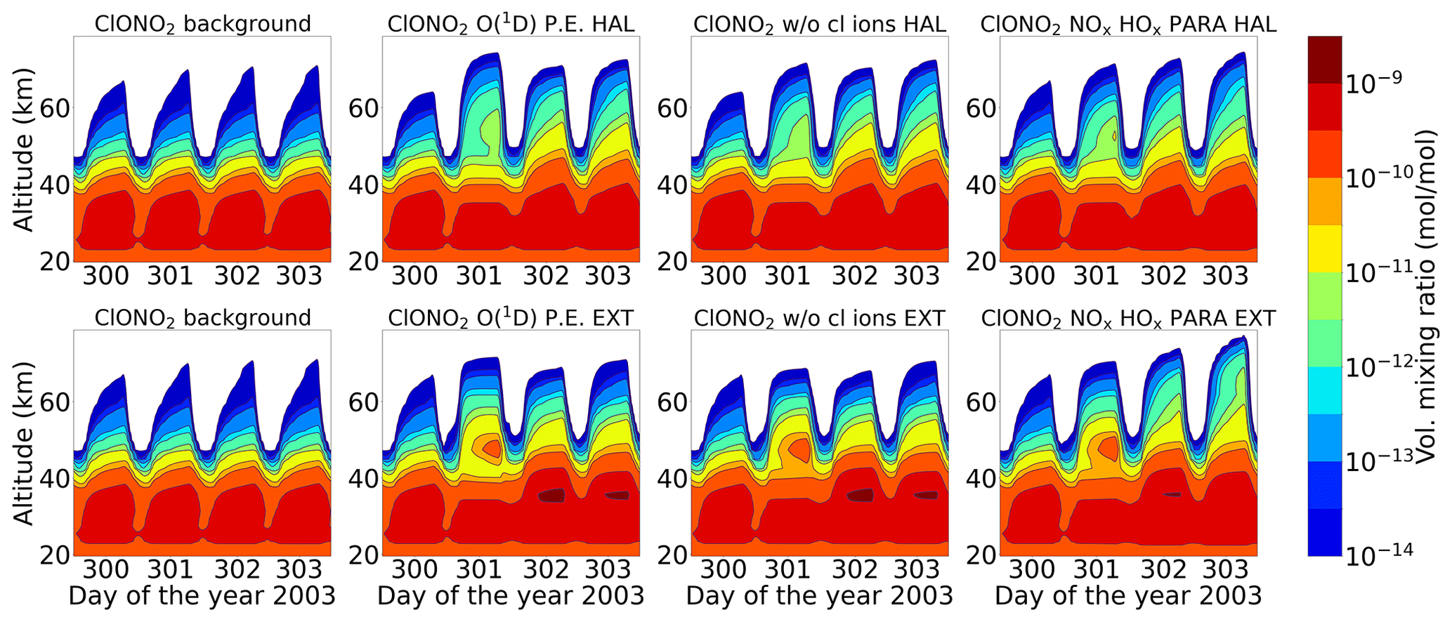
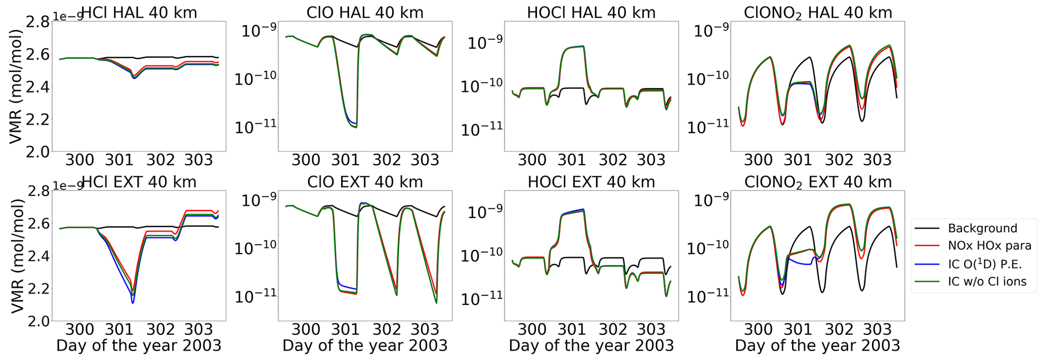
Figure 19 Comparison of the Halloween SPE and the extreme scenario for (column wise) HCl, ClO, HOCl, and ClONO₂ at 40 km.

An increase in ClONO₂ is also observed during both events at an altitude of 60 km (Fig. 18). Solomon et al. (1981) pointed out that the increasing NO_x concentrations after the SPE interact with chlorine species, forming chlorine nitrate at the expense of reactive radicals. This reaction is of importance in the lower and middle stratosphere around 40 km (Jackman et al., 2000) but is not so important at higher altitudes. It can be seen from Fig. 18 that, at an altitude of 40 km, ClONO₂ increases after the event has stopped. This is because after the event ClO is lost via Reaction (R32) since NO_x is formed slowly, accumulating over time. So, the formation of ClONO₂ via Reaction (R32) is slow, leading to high production after the event in the lower and middle stratosphere. The chlorine ion chemistry plays a small role in ClONO₂ around 45–50 km, especially during nighttime on day 301. The production of ClONO₂ when the chlorine ion chemistry is switched off is comparatively higher at that altitude.

Figure 19 shows the chlorine species at an altitude of 40 km for the various model set-ups. There is a small impact of chlorine ion chemistry on the loss of HCl, whereas the parameterized NO_x and HO_x underestimate it. ClO decreases during the event and is converted to HOCl via Reaction (R19). After the event, it recovers, and the HOCl enhancements also decrease. For the extreme event, however, ongoing loss of ClO during nighttime is observed, which is due to the excess HO_x produced during the extreme event. Reformation of HCl after the event is observed, which happens via Reactions (R26) and (R27).

An interesting observation for HCl can be seen in Fig. 19 for the extreme scenario, where the recovered HCl after the event shows a positive excursion. This depends on the diurnal cycle of ClO and happens mainly during nighttime. The reformation of HCl can happen via Reactions (R26) and (R27) during nighttime because, during daytime, HO₂ and H₂O₂ photolyse. This can be seen in Fig. 20, where HO₂ and H₂O₂ production increases during the event, mainly at nighttime. A steep increase in HCl is observed during the transition from day to night where Cl, HO₂, and H₂O₂ increase, which is constant over the night and increases again afterwards at the beginning of the day. This is due to the fact that, during nighttime, the concentration of free chlorine atoms is typically low since the primary source of these atoms is the dissociation of chlorine-containing reservoir species, such as chlorine nitrate (ClONO₂). ClONO₂ occurs predominantly during daytime due to the presence of sunlight, where it is photolysed to release chlorine atoms, and hence at sunrise this renewed increase in chlorine atoms results in a subsequent increase in HCl levels.

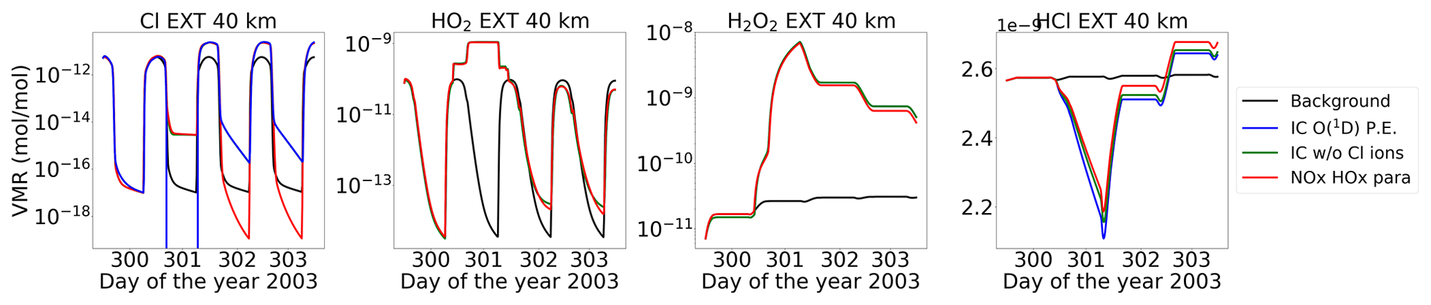
Figure 20 Volume-mixing ratios of species (Cl, HO₂, H₂O₂, and HCl) at 40 km for the extreme event. The different lines are for the model settings: reference (black), ion chemistry with O(¹D) in photo-chemical equilibrium (blue), without chlorine ions (green), and parameterized NO_x and HO_x (red).

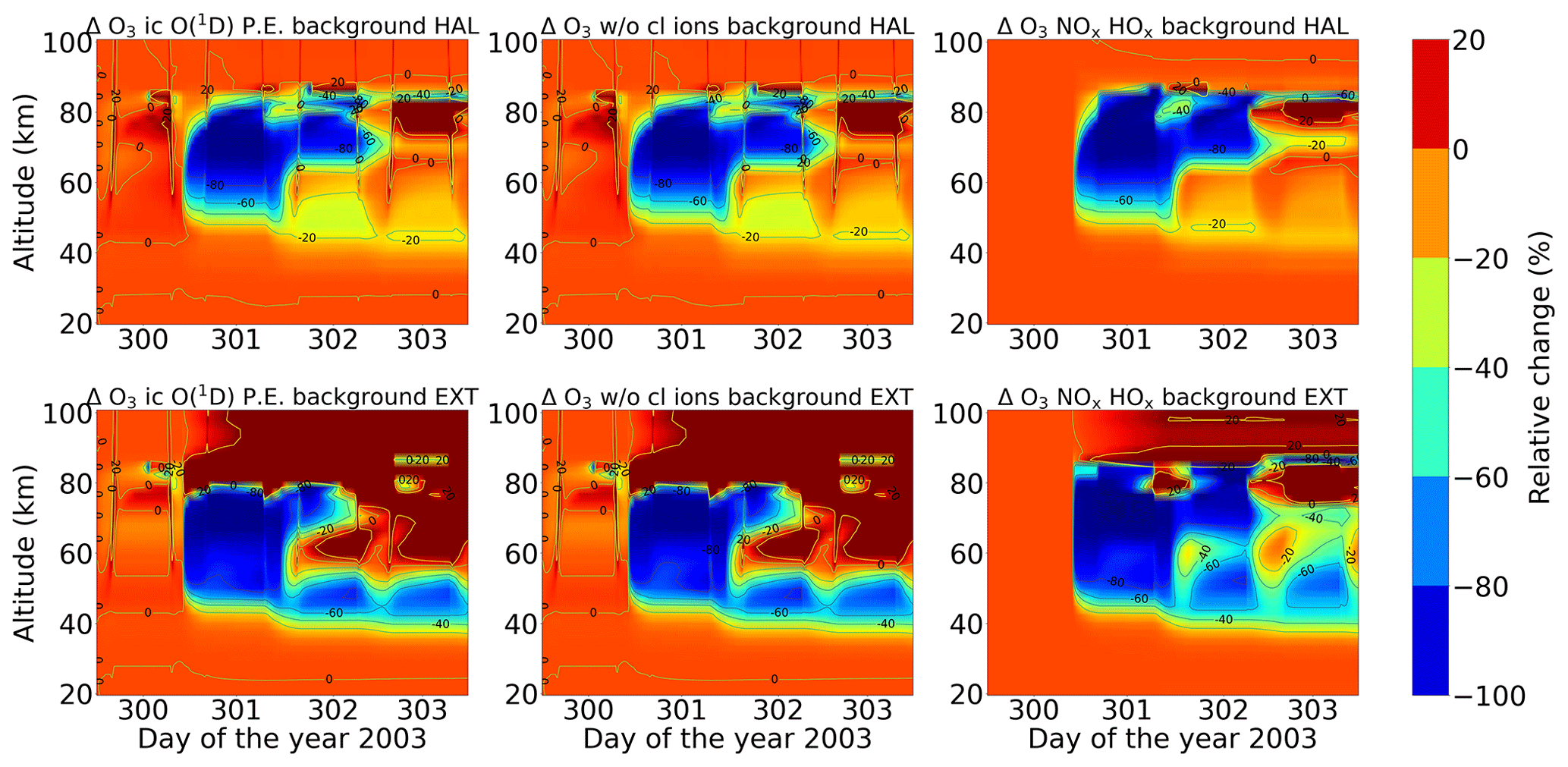
Figure 21 Percentage difference of ozone for the different model runs with respect to the reference run (row-wise): Halloween event and extreme scenario; (column-wise) ion chemistry with O(¹D) in photochemical equilibrium, without Cl ions and parameterized NO_x and HO_x.

4.3 Ozone

Figure 21 shows the percentage difference of ozone for the two events for the different model runs calculated with respect to the reference run. It is seen that, with the onset of the event, ozone is completely lost, which is due to HO_x enhancements in the mesosphere above 55 km. This net ozone loss in the upper stratosphere and mesosphere is mainly due to odd hydrogen (HO_x) catalytic destruction cycles (Reactions R6 and R7) (Jackman et al., 2005) and is short-lived. Since HO_x species have a shorter lifetime, the recovery of ozone is faster. For the extreme event, after the event stops, ozone enhancements of up to 25 % are observed in the mesosphere and above 80 km.

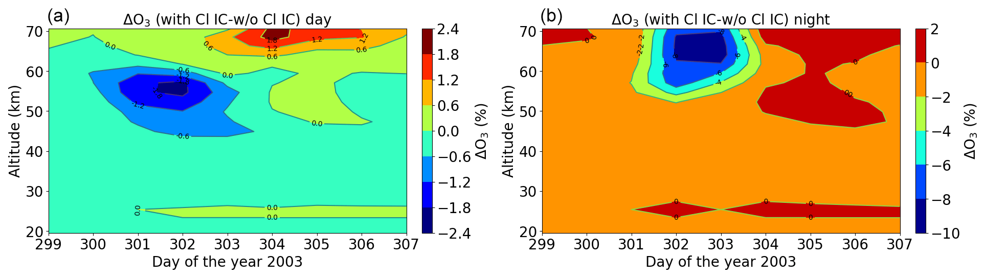
Figure 22 Relative difference of the model with full ion chemistry and O(¹D) in photo-chemical equilibrium, including chlorine ions with respect to the model without chlorine ion chemistry for the Halloween SPE: daytime (a) and nighttime (b). The difference here is calculated for daily averaged data.

NO is quite long-lived down at the 60 km altitude and below, so the ozone loss due to the NO_x catalytic cycle seems to be persistent. The ozone loss occurs during daytime, when NO reacts with ozone to form NO₂, which is then photolysed back to NO, and this catalytic cycle between NO and NO₂ and related to daytime continues (see Reactions R12 and R13). In the beginning, the amount of $\stackrel{\mathrm{̃}}{{\mathrm{NO}}_y}$ was not enough for ozone loss, but at the end of the event, the accumulation is large enough for significant ozone depletion, which stays on and produces a diurnal cycle between 40 and 80 km due to NO_x–HO_x cycles as seen in Fig. 21. The magnitude of depletion with respect to the diurnal cycle and altitude has some considerable variation. Verronen et al. (2005) used a 1D chemical model, the Sodankylä Ion and neutral Chemistry model (SIC) for ionospheric D-region studies. They studied the effects of ion chemistry on the neutral atmosphere, the diurnal variation of NO_x or HO_x increases, and ozone depletions. This diurnal variation during a solar proton event or an EPP event was previously reported by Aikin and Smith (1999). Verronen et al. (2005) observed the diurnal cycle of O_x = O + O₃ depletion between 40 and 85 km. They found substantial ozone loss at sunset on 28 October and even greater loss at sunrise on 29 October followed by a recovery at 55–75 km during the noon and afternoon hours. The maximum depletion is reached just after sunset, with a 95 % reduction in the O_x values at 78 km. During daytime on 30 October, O_x partly recovers but is again depleted during sunset. Rohen et al. (2005) also studied the Halloween SPE using SCanning Imaging Absorption spectroMeter for Atmospheric CHartographY (SCIAMACHY) observations and considered the 60^∘ N magnetic latitude, which compares quite well to our 67.5^∘ N geographic latitude. Since SCIAMACHY only measures during daytime, they did not see a diurnal cycle in their results. With SCIAMACHY, they reported a 20 %–30 % ozone loss at 40–50 km in the Northern Hemisphere during the event and a 20 %–40 % ozone loss (also during the event at 40–55 km observed by a photochemical model). This is related to the NO_x catalytic cycle that was long-lived. Above 50 km and at higher altitudes, ozone recovery was faster after 50 %–60 % loss during the event observed with SCIAMACHY and the model, which was due to the short lifetime of HO_x and photolytical reproduction of ozone. In our case, the continuing ozone loss at 40–55 km related to the diurnal variation of NO_x is found to be 60 %–80 % for the extreme scenario as compared to the Halloween event, which is just around 20 %. At 60–80 km, 80 %–100 % ozone loss is observed during the event and the continuing loss due to the HO_x-related diurnal cycle afterwards. Two other examples that provide valuable insights into the significant ozone variations that can occur during extreme space weather events were studied by Calisto et al. (2013) and Rodger et al. (2008). Calisto et al. (2013) investigated the potential effects of a Carrington-like solar event on ozone using a global 3D chemistry-climate model (SOCOL v2.0). They found that the enhanced ionization during the event led to substantial ozone depletion in the polar regions, particularly in the middle atmosphere. Due to the NO_x and HO_x enhancements, ozone depletion was found to be 60 % in the mesosphere and 20 % in the stratosphere for several weeks after the event started. They also showed that total ozone decreased by more than 20 DU in the Northern Hemisphere. Rodger et al. (2008) examined the relationship between SPEs and ozone depletion using ground-based observations and modelling. They used the SIC model, investigated the Carrington event of August and September 1859, and found that SPEs can cause localized ozone depletion in the polar regions, primarily through the production of NO_x. The most important SPE-driven atmospheric response is an unusually strong and long-lived O_x decrease in the upper stratosphere (O_x levels drop by 40 %) primarily caused by the very large fluxes of >30 MeV protons. Considering these studies, it is crucial to recognize that the ion chemistry processes during SPEs can lead to ozone changes that go beyond what is typically captured in fixed parameterizations or standard models. The enhanced ionization and subsequent chemical reactions can influence ozone concentrations, particularly in the polar regions. Therefore, when studying the impact of SPEs on ozone, it is important to consider the effects of ion chemistry processes and their potential role in generating substantial ozone variations. By incorporating these processes into models, we can better understand the complex interplay between extreme space weather events, ion chemistry, and ozone dynamics, ultimately improving our ability to assess the impacts of such events on Earth's atmosphere.

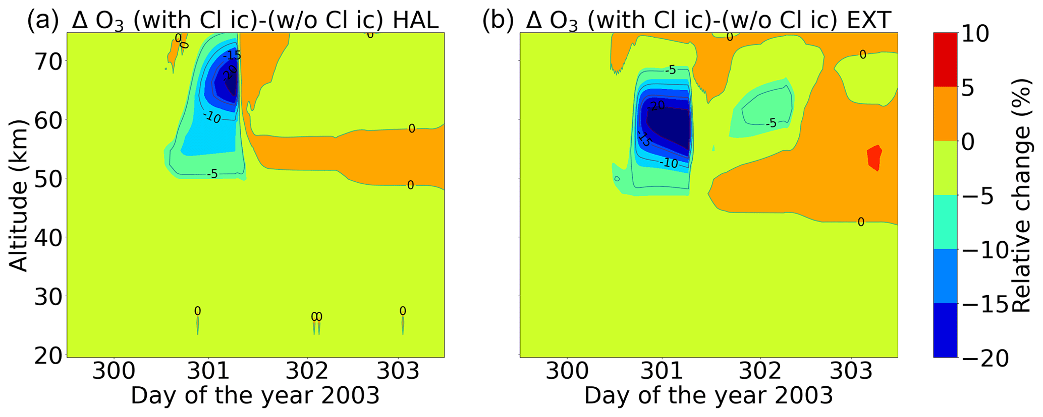
Figure 23 Relative difference of the model simulations: full ion chemistry with O(¹D) in photo-chemical equilibrium and with chlorine ions with respect to the model setting without chlorine ion chemistry, comparing the Halloween SPE (a) and the extreme scenario (b). The data shown here are not daily averaged but are the real model time step.

5 Impact of chlorine ions on ozone loss

The evaluation of the model results with MIPAS observations gave us confidence in the model. Thus, the impact of chlorine ion chemistry on ozone loss could be assessed using the model. According to the model, we found the ozone loss in the stratosphere and lower mesosphere during the event. Figure 22 shows the relative difference of the ion chemistry model with O(¹D) in photo-chemical equilibrium, including chlorine ions with respect to the model without chlorine ions for daytime and nighttime. The difference in this case is calculated here for daily averaged data for each day. Losses of 2.5 % during daytime in an altitude range of 40–60 km and about 10 % during nighttime at an altitude of 50–70 km are observed during the event day. Negative chlorine species directly increase the concentrations of uncharged active chlorine compounds. Through their catalytic cycles, these uncharged chlorine compounds can be responsible for ozone loss at different altitudes that is also dependent on illumination conditions. The ClO_x catalytic cycle (Reactions R15 and R16) is responsible for the ozone loss at 40–50 km. There is a slight difference between daytime and nighttime in the loss observed in terms of altitude range, which is expected. This difference can be explained by the difference in the diurnal cycle of ClO during daytime and nighttime. The catalytic ozone loss cycles relevant in the stratosphere and mesosphere are ClO + O (Reactions R15–R17) and ClO + HO₂ (Reactions R18, R19, and R21), which also need solar light since O is formed by photolysis. During daytime, ClO photolyses in the mesosphere but not in the stratosphere, so ClO is not observed in the mesosphere. The ClO + HO₂ cycle produces HOCl, which also photolyses during daytime and produces Cl through Reaction (R20). So, during daytime, Cl is more important than ClO. However, during nighttime, ClO accumulates in the mesosphere and in the stratosphere; this is mainly ClONO₂ due to Reaction (R32). As we see from our results, during the event days on 28 October and 29 October, the ClO mixing ratios were found to be higher for nighttime around 60–70 km compared to daytime. Hence, the ozone loss occurs more in the upper stratosphere or mesosphere around 50–70 km for nighttime, thereby producing the difference in the ozone loss in the altitude range. Losses of 0.6 % during daytime and 2 % during nighttime are observed in the altitude range 30–40 km. The ClO_x cycles with Reactions (R28)–(R30) and Reactions (R32)–(R35) are responsible in this altitude range for both daytime and nighttime. Furthermore, a continuous ozone formation of 2 % during both daytime and nighttime is observed. This increase is linked to enhanced atomic oxygen production by O₂ photolysis in solar maximum conditions (Marsh et al., 2007). It is observed in altitude ranges of 60–70 km for daytime and 50–70 km for nighttime.

Figure 23 shows the relative differences in the model setting, with ion chemistry and O(¹D) in photo-chemical equilibrium with respect to the model setting without chlorine ion chemistry comparing the Halloween SPE and the extreme event in order to assess the impact of chlorine ion chemistry on ozone loss during the event day. An impact of the chlorine ions around 10 %–20 % is observed on the event day. Qualitatively, it was a bit more for the extreme event compared to the Halloween SPE, which could be more important for higher forcing. An increase of around 5 % for ozone is also seen after the event stops for the extreme scenario. The extreme run does not show any impact of chlorine ion chemistry on ozone loss at 70–75 km, while the Halloween SPE does. This can be explained by the ClO and HOCl responses to SPEs as well as by the ClO_x catalytic cycle. At an altitude of 70–75 km, ClO decrease for the sensitivity runs for both ion chemistry with O(¹D) in photo-chemical equilibrium and without chlorine ions is larger for the extreme event compared to the Halloween SPE (Fig. 16). This is one contributing factor as to why we do not see an impact on ozone loss at these altitudes. Kalakoski et al. (2020) used WACCM-D to investigate ozone depletion around 50–60 km after the onset of the SPE as explained in Sect. 4. They studied the effect in both hemispheres, and the duration and altitude range of this extra ozone loss correspond to NO_x and enhanced Cl_x(= Cl + ClO) mixing ratios. An ozone loss of 0.2 ppm in both hemispheres was observed after the event. Around 70 km, the ozone loss was due to short-lived HO_x. Around 50 km, it is driven by NO_x and Cl_x and lasts longer, with a maximum ozone decrease seen about 30 d after the event onset. Since HCl responses to SPEs are partly due to chlorine ion chemistry, which converts it to Cl, ClO, and HOCl (Winkler et al., 2009), this is also indirectly an effect of the chlorine ion chemistry. They also see an increase in ozone around 0.2 ppm throughout the period near the secondary ozone maximum above 80 km, which is also due to the O₂ photolysis as discussed above. We observe a continuous increase in O₃ after the event, which is about 5 %. This increase was seen around 50–60 km for the Halloween SPE and around 50–75 km for the extreme scenario.

6 Discussions and conclusions

Using satellite data (MIPAS on ENVISAT), the state-of-the-art 1D ion chemistry ExoTIC model has been validated. Two event classes were modelled, and chlorine ion chemistry and its impact on ozone were evaluated. ExoTIC was used to study the short-term constituent changes caused by the Halloween SPE of 2003. The results demonstrated here show a comparison of stratospheric and mesospheric composition changes observed by MIPAS in the polar cap region with simulations performed by ExoTIC. The inter-comparison of the model and MIPAS observations allowed for an evaluation of the overall ability of the ExoTIC model to reproduce observed atmospheric perturbations generated by solar proton events, particularly with respect to changes in the chlorine species, SPE-induced NO_y enhancements, and ozone depletion. Polar upper-stratospheric and lower-mesospheric NO_y increased by over 40 ppbv, and mesospheric ozone decreased by over 70 % during the SPE period. The inter-comparison also tested and identified deficiencies in the chemical schemes, particularly with respect to nitrogen and chlorine chemistry, which is relevant for stratospheric ozone. Short-term enhancements of HOCl and ClONO₂ were observed by MIPAS and also reproduced in the simulations with different model settings. Application of MIPAS averaging kernels to the ExoTIC output made the inter-comparison much better. HOCl enhancements were reproduced best for the model simulation with ion chemistry, where O(¹D) was set to photo-chemical equilibrium. An HOCl enhancement of more than 0.2 ppbv occurred roughly during the event as observed by MIPAS. The HOCl enhancements with averaging kernels as found in ExoTIC and its temporal variation agree quite well with MIPAS. The ozone depletion simulated by the model extends over a large altitude range as compared to MIPAS observations. Jackman et al. (2008) found the opposite from WACCM3 results in the Northern Hemisphere in terms of altitude range. The encountered differences between the model and observations for ClONO₂ enhancements (its underestimations by the model) are related to a smaller availability of ClO in the polar region before the SPE. The ClONO₂ peak is observed at the same altitude for both the model and MIPAS, but the enhancements in MIPAS are observed earlier, and the peak values seem to agree quite well even without the averaging kernels applied. Jackman et al. (2008) also found the ClONO₂ peak at the same altitude with WACCM3, but the values were underestimated by a factor of 2 compared to MIPAS.

The comparison of the Halloween SPE and the extreme solar event of AD 775 showed long-lasting stratospheric ozone loss for the extreme scenario. A long-lasting impact was also found for chlorine species like HOCl and HCl in the case of the extreme scenario. Loss of HCl was underestimated by the parameterized model, which was also found by Winkler et al. (2009) during the solar proton event in July 2000 in the northern polar region. For the extreme event, the parameterized model showed much higher NO_y enhancements, about 1000 ppm in the mesosphere and lower thermosphere. HO_x enhancements of 0.1 ppm were found during the extreme event, which went further down in altitude up to 40 km for all the model case studies. An impact of around 10 %–20 % on ozone loss was found due to the chlorine ions for the two events, which is a bit stronger for the extreme scenario and is more important for higher forcing. Ozone formation was observed after the event, which is also due to the impact of chlorine ion chemistry. For the Halloween event with temporal ionization rates, ozone losses of 2.4 % during daytime and 10 % during nighttime were observed during the event, which is also due to the included chlorine ion chemistry. Ozone formation of 2 %–4 % was found after the event during both daytime and nighttime.

In general, ExoTIC simulations reproduced the impacts of the Halloween SPE quite well, mainly for HOCl and NO_y. However, the initial state of the atmosphere in the simulations could be an important factor for some variability in the model results and MIPAS observations. Future work will focus on including the D-region ion chemistry in the global 3D chemistry-climate model EMAC and the evaluation of the chemistry with MIPAS observations in a set-up considering atmospheric dynamics. While previous results with UBIC focused on the solar proton event in July 2000 in the northern polar region and compared them to the HCl measurements from the Halogen Occultation Experiment instrument (HALOE), we compare the results of the ion-chemistry model simulations with MIPAS observations. Since MIPAS observations provide a better picture of the polar cap region as compared to HALOE observations that are less densely sampled, these results suggest that the validated D-region ion chemistry set-up in the ExoTIC model can be trusted for implementation in a global 3D model. The problem of O(¹D) in the ion chemistry in ExoTIC should be taken into account, which was however related to the neutral chemistry model as explained in Sect. 2.2.1. For a global 3D chemistry-climate model, at least in EMAC, which we are considering for the implementation, the ion chemistry is part of the normal chemistry solver, and in that case, the O(¹D) formation rate should not be too large and should work without doing anything to O(¹D). This set-up will first be evaluated with MIPAS observations and, since EMAC can already provide the data at the MIPAS footprints, the modelled data can be sampled at MIPAS measurement local times. The model will then be considered for experiments in different set-ups to look at the dynamical impacts with and without the D-region ion chemistry with important chemical reactions involving water, chlorine, and NO⁺ cluster ions.

Appendix A: Chlorine ions and ionic reactions

In this Appendix, the reactions involving the chlorine ions and their rate coefficients used in ExoTIC are listed.

Amelynck et al. (1994)Kopp and Fritzenwallner (1997)Turco (1977)Kazil et al. (2003)Kopp and Fritzenwallner (1997)Kopp and Fritzenwallner (1997)Kopp and Fritzenwallner (1997)Kopp and Fritzenwallner (1997)Kopp and Fritzenwallner (1997)Turco (1977)Huey (1996)Turco (1977)Amelynck et al. (1994)Kopp and Fritzenwallner (1997)Kopp and Fritzenwallner (1997)Kopp and Fritzenwallner (1997)Kopp and Fritzenwallner (1997)Kopp and Fritzenwallner (1997)Kopp and Fritzenwallner (1997)Kopp and Fritzenwallner (1997)Turco (1977)Amelynck et al. (1994)Kopp and Fritzenwallner (1997)Kopp and Fritzenwallner (1997)Amelynck et al. (1994)Kopp and Fritzenwallner (1997)Kopp and Fritzenwallner (1997)Kopp and Fritzenwallner (1997)Kopp and Fritzenwallner (1997)Kopp and Fritzenwallner (1997)Kopp and Fritzenwallner (1997)Amelynck et al. (1994)Turco (1977)Turco (1977)Turco (1977)Turco (1977)Turco (1977)Turco (1977)Turco (1977)Turco (1977)Turco (1977)Turco (1977)Turco (1977)Turco (1977)Turco (1977)Turco (1977)Turco (1977)Turco (1977)Turco (1977)Turco (1977)Turco (1977)Turco (1977)Turco (1977)Turco (1977)Arijs et al. (1987)

Table A1 T is the temperature (K), and M is the total air density (cm⁻³).

^* The coefficient is the same for all the reactions below.