the Creative Commons Attribution 4.0 License.
the Creative Commons Attribution 4.0 License.
 | 09 Oct 2023
A roadmap to estimating agricultural ammonia volatilization over Europe using satellite observations and simulation data
Camille Viatte
William C. Porter
Nikolaos Evangeliou
Cathy Clerbaux
Lieven Clarisse
Martin Van Damme
Pierre-François Coheur
Sarah Safieddine
Ammonia (NH3) is one of the most important gases emitted from agricultural practices. It affects air quality and the overall climate and is in turn influenced by long-term climate trends as well as by short-term fluctuations in local and regional meteorology. Previous studies have established the capability of the Infrared Atmospheric Sounding Interferometer (IASI) series of instruments, aboard the Metop satellites, to measure ammonia from space since 2007. In this study, we explore the interactions between atmospheric ammonia, land and meteorological variability, and long-term climate trends in Europe. We investigate the emission potential (Γsoil) of ammonia from the soil, which describes the soil–atmosphere ammonia exchange. Γsoil is generally calculated in-field or in laboratory experiments; here, and for the first time, we investigate a method which assesses it remotely using satellite data, reanalysis data products, and model simulations.
We focus on ammonia emission potential in March 2011, which marks the start of growing season in Europe. Our results show that Γsoil ranges from 2 × 10³ to 9.5 × 10⁴ (dimensionless) in fertilized cropland, such as in the North European Plain, and is of the order of 10–102 in a non-fertilized soil (e.g., forest and grassland). These results agree with in-field measurements from the literature, suggesting that our method can be used in other seasons and regions in the world. However, some improvements are needed in the determination of mass transfer coefficient k (m s−1), which is a crucial parameter to derive Γsoil.
Using a climate model, we estimate the expected increase in ammonia columns by the end of the century based on the increase in skin temperature (Tskin), under two different climate scenarios. Ammonia columns are projected to increase by up to 50 %, particularly in eastern Europe, under the SSP2-4.5 scenario and might even double (increase of 100 %) under the SSP5-8.5 scenario. The increase in skin temperature is responsible for a formation of new hotspots of ammonia in Belarus, Ukraine, Hungary, Moldova, parts of Romania, and Switzerland.
- Article
(12409 KB) - Full-text XML
- Companion paper
-
Supplement
(1451 KB) - BibTeX
- EndNote


Ammonia (NH3) emissions increased in a continuous manner from 1970 to 2017 (McDuffie et al., 2020). During the period 2008–2018 alone, the increase in ammonia columns in western and southern Europe amounted to 20.8 % yr−1 (± 4.3 %) and to 12.8 % yr−1 (± 1.3 %) globally (Van Damme et al., 2021). Although ammonia alone is stable against heat and light, it is considered to be a very reactive base, and it constitutes the largest portion of the reactive nitrogen (Nr) on Earth. The vast majority of atmospheric ammonia that is not deposited is transformed into fine particulate matter (PM2.5) composed of ammonium (), through acid–base chemical reactions with available acids in the environment, namely sulfuric acid (H2SO4), hydrochloric acid (HCl), and nitric acid (HNO3) (Yu et al., 2018), while only 10 % of the total ammonia gas is believed to be oxidized by hydroxyl radicals (OH−) (Roelle and Aneja, 2005). PM2.5 has degrading effects on human health, especially respiratory diseases (Bauer et al., 2016). Soils are known to be a source of atmospheric ammonia, especially in areas of intensive agricultural practices (Schlesinger and Hartley, 1992), and this is due to enrichment of the soil with the reactive nitrogen present in fertilizers. The increase in the application of synthetic fertilizers and intensification of agricultural practices are believed to be the dominant factors of the global increase in ammonia emissions over the past century (Behera et al., 2013; McDuffie et al., 2020). In addition to agriculture, ammonia can be emitted from industrial processes, biomass burning (Van Damme et al., 2018), and natural sources such as from seal colonies (Theobald et al., 2006).
Following the application of fertilizers, ammonium and ammonia are released in the soil. Prior to its volatilization, ammonia in the soil exists in either the gas phase (NH3 (g)) or the aqueous/liquid phase (NH3 (aq)); the equilibrium between both states of ammonia is governed by Henry's law (Wentworth et al., 2014), as shown in the Appendix A. The dissociation of ammonia in soil water is a function of soil acidity (pH) and temperature (Roelle and Aneja, 2005) (Eqs. A1 and A2 in Appendix A) and controlled by the dissociation constant . Once released to the atmosphere, ammonia near the surface exists in the gas phase; hence Henry's law can be used to describe the equilibrium between ammonia in the soil (liquid phase) and near the surface (gas phase). This bidirectional exchange between the soil and the atmosphere will continue until the equilibrium is reached, and this occurs when ammonia concentration is equal to the compensation point (the concentration of ammonia at equilibrium). The flux of ammonia from the soil to the atmosphere (emission) occurs when the concentration of atmospheric ammonia is less than the compensation point , while ammonia deposition occurs when the concentration of ammonia is equal to or greater than (Flechard et al., 2011; Wichink Kruit, 2010). It is then crucial to quantify the compensation point in order to understand this bidirectional exchange. The main variables needed to calculate are soil temperature (Tskin) and Γsoil, which is a dimensionless ratio between ammonium and pH ( and H+ (aq) concentrations, respectively, in the soil). All the equations are described in Appendix A (Eqs. A1 to A15).
The soil emission potential (Γsoil) has been thoroughly investigated in field and controlled laboratory environments (e.g., David et al., 2009; Flechard et al., 2013; Massad et al., 2010; Mattsson et al., 2009; Nemitz et al., 2000; Wentworth et al., 2014; among others). Γsoil is dimensionless, and it can range from 20 (non-fertilized soil in a forest) to a value on the order of 106 (mixture of slurry in a cropland). It is found to peak right after fertilizer application, due to the increase in ammonium content in the soil (a product of urea hydrolysis), and to return to pre-fertilization levels 10 d after the application (Flechard et al., 2010; Massad et al., 2010). Little information exists on regional or global scales to assess the large-scale spatial variability in ammonia emission potentials.
In order to meet the needs of a growing population, agricultural practices intensified during the 2003–2019 period (more fertilizer use per surface area), resulting in increased net primary production (NPP) per capita (Potapov et al., 2022) and volatilized ammonia (due to an increase in both nitrogen soil content and cultivated lands). In Europe alone, the area of croplands increased by 9 % from 2003 to 2019, and most of the expansion took place on lands that were abandoned for more than 4 years (Potapov et al., 2022). Around 90 % of the mineral fertilizers used in Europe are nitrogen-based, with urea and nitrate fertilizers dominating the market in the 27 EU countries, since they make up 22 % and 45 % of the total market (Fertilizers Europe, 2016). With the increase in cropland area and agricultural activities, climate change will have a significant effect on agricultural practices, with warmer climates enhancing the volatilization of ammonia from soils, especially in intensely fertilized lands (Shen et al., 2020).
This study aims at exploring ammonia emission potential and volatilization in Europe, using infrared satellite data of ammonia columns, reanalysis temperature data, and chemical transport model simulations to provide information on chemical sources and sinks. We specifically study the relationship between satellite-derived ammonia concentration at the start of the growing season, soil emission potentials, and their spatial variability over Europe in March of 2011. Section 2 provides the methods and datasets used. The results are described in Sect. 3, including simulation from GEOS-Chem in Sect. 3.1. Regional emission potentials are shown and discussed in Sect. 3.2. Using a climate model, future projections of ammonia columns are investigated under different climate scenarios in Sect. 3.3. Conclusions are listed in Sect. 4.
2.1 Calculation of the emission potential
In this study, we use Infrared Atmospheric Sounding Interferometer (IASI) satellite data to calculate the ammonia emission potential Γsoil instead of field soil measurements. In field studies, Γsoil is calculated by measuring the concentration of ammonium () and H+ (10−pH) in the soil; the ratio between both of these concentrations is Γsoil. Here, we use infrared satellite observations, which offer a regional coverage over Europe. With these, however, we cannot monitor soil content of ammonium nor its pH. This renders the remote Γsoil calculation challenging and less straightforward. The full derivation of the equation used to calculate the emission potential is explained in Appendix A. In short, upon its dissolution in the soil water, ammonia follows Henry's law. In steady-state conditions between the soil and the near surface, the amount of the ammonia emitted and lost is considered equal. Based on this assumption, the soil emission potential (dimensionless) is calculated as shown in Eqs. (1) and A15 in Appendix A:
where is the total column concentration of ammonia (), measured by satellite remote sensors; Tsoil is the soil temperature at the surface, which can be expressed as the skin temperature Tskin (Kelvin); a and b are constants (a = 2.75 × 10³ g K cm−3, b = 1.04 × 10⁴ K); is the molar mass of ammonia (M = 17.031 g mol−1); Na is Avogadro's number (Na = 6.0221409 × 10²³ ); c′ is 100 and is added to convert k from meters per second to centimeters per second (since is in molecules per square centimeter); and τ is the lifetime of ammonia (seconds).
The term k is the soil–atmosphere exchange coefficient or deposition velocity (cm s−1), also known as the mass transfer coefficient (this nomenclature is used in this study). It is a function of the roughness length of the surface, wind speed, boundary layer height (Olesen and Sommer, 1993; Van Der Molen et al., 1990), and pH (Lee et al., 2020). It can also be calculated using a resistance model, often used to explain the exchange between the surface and the atmosphere (Wentworth et al., 2014). Different studies provide look-up-table values of k for different land cover types and different seasons based on this resistance model (Aneja et al., 1986; Erisman et al., 1994; Phillips et al., 2004; Roelle and Aneja, 2005; Svensson and Ferm, 1993; Wesely, 1989).
In general, the mass transfer coefficient k is on the order of 10−3 to 10−2 m s−1 in a mixture of soil and manure and 10−6 to 10−5 m s−1 in a mixture of manure alone (Roelle and Aneja, 2005). We discuss and provide more information on k in Sect. 3.2, and additional details on this calculation in general are provided in Appendix A.
2.2 IASI ammonia, ERA5 Tskin, and MODIS land cover
The Infrared Atmospheric Sounding Interferometer (IASI) is considered to be the most innovative instrument on board the polar-orbiting Metop satellites (Klaes, 2018). Three IASI instruments are on board Metop-A, Metop-B, and Metop-C, the series of satellites launched by the EUMETSAT (European Organization for the Exploitation of Meteorological Satellites) in 2006, 2012, and 2018, respectively. The Metop-A satellite was de-orbited in October 2021 (Lentze, 2021), and as a result only two instruments (IASI-B and IASI-C on board Metop-B and Metop-C) are operating today. The observations from IASI cover any location on Earth at 09:30 and 21:30 local solar time. It can detect a variety of atmospheric species including trace gases (Clerbaux et al., 2009). The IASI Fourier-transform spectrometer monitors the atmosphere in the spectral range between 645 and 2760 cm−1 (thermal infrared) and is nadir-looking. IASI has a swath width that measures 2200 km, with a pixel size of ∼ 12 km.
Ammonia was first detected with IASI using the ν2 vibrational band (∼ 950 cm−1) (Clerbaux et al., 2009; Coheur et al., 2009). The ammonia total columns used in this study are the product of an artificial neural network and reanalyzed temperature data from the European Centre for Medium-Range Weather Forecasts (ECMWF) product ERA5 ANNI-NH3-v3R-ERA5 (Van Damme et al., 2021). Several studies used ammonia data from IASI to study hotspots of ammonia of different source types, including both natural and anthropogenic sources (Clarisse et al., 2019a, b; Dammers et al., 2019; Van Damme et al., 2018, 2021; Viatte et al., 2021). Recently, IASI observations were used to study the effect of war and conflict on agricultural practices in Syria (Abeed et al., 2021).
Fewer errors on the retrieval were observed during the day and over land (Van Damme et al., 2017); hence, we use only daytime ammonia measurements from IASI. Comparisons with ammonia measured using a ground-based instrument showed a good correlation of R = 0.75 (Viatte et al., 2021). Satellite ammonia data from CrIS (Crosstrack Infrared Sounder) (Shephard and Cady-Pereira, 2015) were compared with those from IASI and were equally found to give similar results when looking at concentrations from a wildfire (Adams et al., 2019), showing consistency when studying seasonal and interannual variability (Viatte et al., 2020).
In addition to ammonia, we look at skin temperature (Tskin) or land surface temperature (LST) data from the ECMWF reanalysis (ERA5) at a grid resolution of 0.25∘ × 0.25∘ (Hersbach et al., 2020). ERA5 temperatures are interpolated temporally and spatially to the IASI morning overpass (∼ 09:30 local time), since we only consider daytime ammonia. ERA5 temperature data are also used in the retrieval process of the ammonia data we used in this study; the name of the ammonia data product is NH3-v3R-ERA5 (Van Damme et al., 2021). Tskin is defined as the temperature of the uppermost surface layer when radiative equilibrium is reached. It also represents the theoretical temperature required in order to reach the surface energy balance (ECMWF, 2016). Skin temperature in Europe varies with a standard deviation of the daily average that is mostly between 2 and 6 ∘C in northern, central, western, and southwestern Europe and between 4 to 8 ∘C in eastern Europe (not shown here).
In order to assign a mass transfer coefficient k to each land type, we used data from the Moderate Resolution Imaging Spectroradiometer (MODIS), a series of instruments orbiting the Earth aboard the Aqua and Terra satellites. The data product MCD12Q1 (version 6) is a combined Aqua–Terra land cover type product, with a spatial resolution of 500 m. This product provides maps of land cover type from 2001 through 2019 (Sulla-Menashe and Friedl, 2018). From the land use categories included in the MOD12Q1 product (Belward et al., 1999) we focus on croplands, forests, shrublands, and grasslands. We do not include bare lands, snow cover, and urban areas in our analysis; we are not interested in studying these surfaces, since we focus on ammonia volatilization from the soil in areas where fertilizers are applied. In addition to croplands, in this study we show the emission potential in forests and grasslands/shrublands for comparison with values in the literature. In an attempt to calculate an emission potential (Eq. 1) that is relevant to the land cover/use, we therefore assign a mass transfer coefficient k to each land type based on literature values (Aneja et al., 1986; Erisman et al., 1994; Roelle and Aneja, 2005; Svensson and Ferm, 1993; Wesely, 1989), and we discuss it in Sect. 3.2.
2.3 Model simulations
2.3.1 GEOS-Chem chemistry transport model
In this study we use version 12.7.2 of the GEOS-Chem chemical transport model (Bey et al., 2001). The model is driven by the Modern-Era Retrospective Analysis for Research and Applications version 2 (MERRA-2) reanalysis product, including nested domains over Europe at a 0.5∘ × 0.625∘ horizontal resolution. MERRA-2 is the second version of the MERRA atmospheric reanalysis product by the NASA Global Modulation Assimilation Office (GMAO) (Gelaro et al., 2017). Boundary conditions for the nested domains are created using a global simulation for the same months at 2∘ × 2.5∘ resolution. We generate model output for March of 2011, preceded by 1 month of discarded model spin-up time for the nested run and 2 months for the global simulation. March corresponds well to the beginning of the growing season (FAO, 2022; USDA, 2022) and as such to the month of fertilizer application in Europe.
Output includes the hourly mean for selected diagnostics. Anthropogenic emissions are taken primarily from the global Community Emissions Data System (CEDS) inventory (Hoesly et al., 2018). Biogenic non-agricultural ammonia, as well as ocean ammonia sources, are taken from the Global Emission Inventories Activities database (GEIA; Bouwman et al., 1997). Open-fire emissions are generated using the GFED 4.1s inventory (Randerson et al., 2015). We used the Harmonized Emissions Component module (HEMCO) to obtain the ammonia emissions over Europe (Keller et al., 2014).
2.3.2 EC-Earth climate model
To analyze how future climate will affect ammonia concentration and emission potential, we use the ECMWF European Earth Consortium climate model (EC-Earth; http://www.ec-earth.org/, last access: 26 September 2023). While other climate models exist, we choose this one because the ammonia product from IASI uses ERA5 for the retrievals, and we calculate the emission potential from the Tskin product of ERA5. The reanalysis uses the ECMWF Integrated Forecasting System for the atmosphere–land component (IFS). The IFS is also used in EC-Earth and is complemented with other model components to simulate the full range of Earth system interactions that are relevant to climate (Döscher et al., 2022). We note that the versions of the IFS models used in ERA5 and in EC-Earth are not identical as the climate model product is not assimilated and is not initialized with observations several times a day like ERA5. The EC-Earth simulations are included in the Climate Model Intercomparison Project Phase 6 (Eyring et al., 2016), part of the Intergovernmental Panel on Climate Change (IPCC) report of 2021 (Masson-Delmotte et al., 2021). We use the so-called Scenario Model Intercomparison Project (ScenarioMIP), covering the period 2015–2100 for future projections under different shared socio-economic pathways (SSPs) (Riahi et al., 2017). We analyze two scenarios: the SSP2-4.5, a “middle-of-the-road” socio-economic scenario with a nominal 4.5 W m−2 radiative forcing level by 2100, similar to the RCP-4.5 scenario, and the SSP5-8.5, the upper edge of the SSP scenario spectrum with a high fossil-fuel-development use over the 21st century.
2.4 GEOS-Chem validation with IASI
To analyze how well the model simulates atmospheric ammonia, we compare the simulated GEOS-Chem hourly averaged (March 2011) ammonia total column output (Sect. 2.3.1) with the IASI NH3 total columns gridded at the same horizontal resolution (0.5∘ × 0.625∘) and during the same month. We applied a temporal coincidence criterion to GEOS-Chem outputs in order to compare them with IASI morning observations. For instance, we selected data between 08:30 and 11:30 UTC in the GEOS-Chem model output.
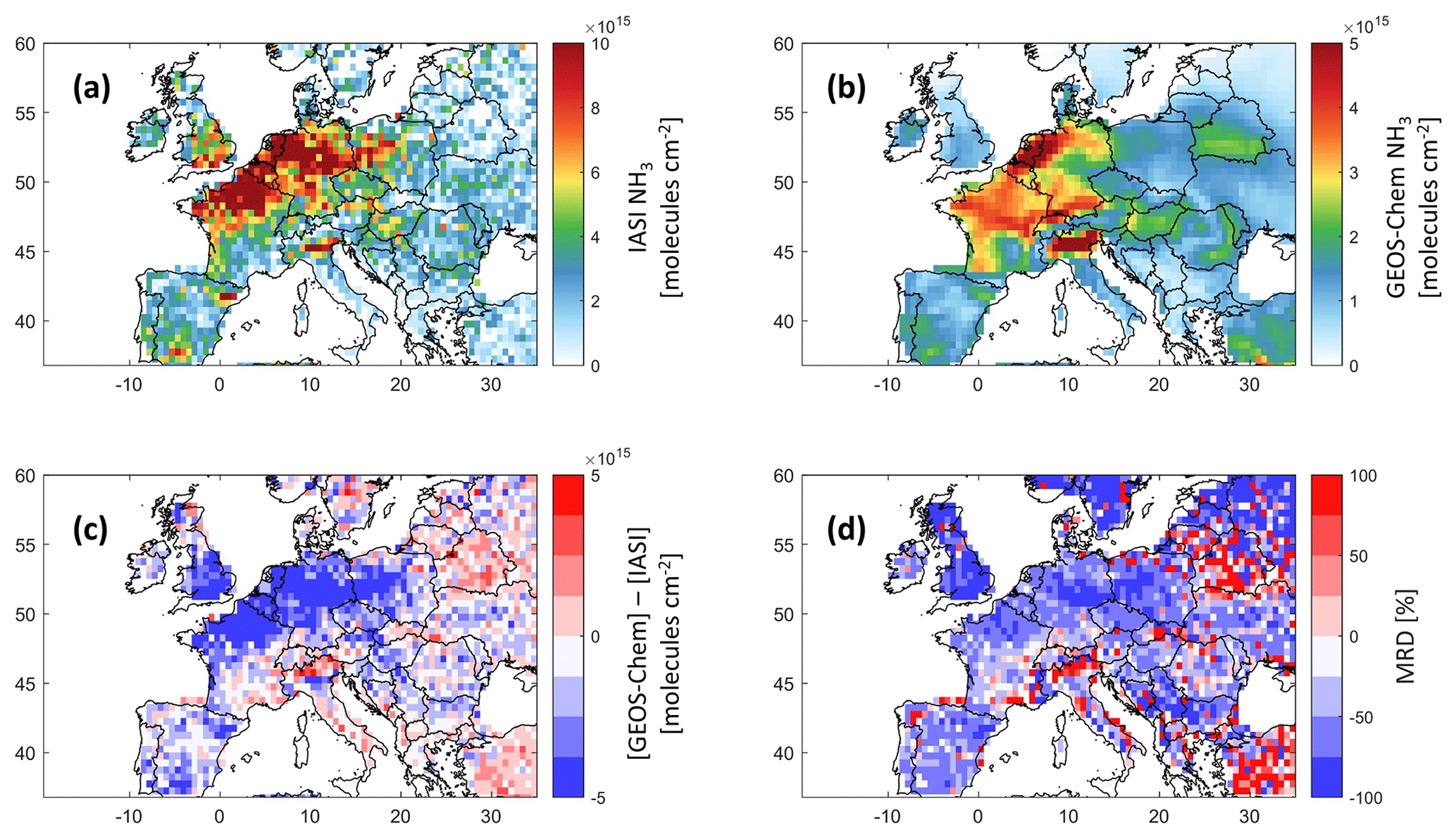
Figure 1Ammonia total column concentrations from IASI (a) and GEOS-Chem (b), the difference between both datasets (c) in molecules per square centimeter, and the mean relative difference (MRD) in percent (d); all data are a monthly average of March 2011 at a 0.5∘ × 0.625∘ grid resolution. Note that the color bar limits are different between (a) and (b).
Figure 1 shows the IASI NH3 distribution (Fig. 1a) and that from GEOS-Chem (Fig. 1b), the bias between the two (Fig. 1c), and the mean relative difference MRD (Fig. 1d), all in March 2011. MRD is calculated as the mean of the ratio at each grid point.
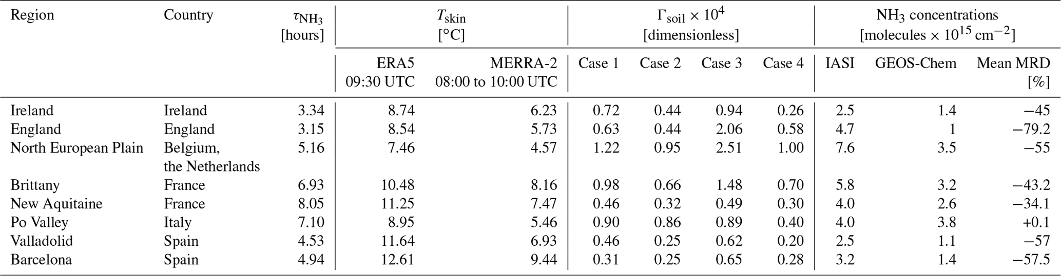
Table 1Summary of ammonia average lifetime, emission potential, concentrations, and the Tskin in selected regions in Europe.
Generally, both GEOS-Chem and IASI show coincident sources of ammonia, reflecting the good ability of the model to reproduce ammonia columns over major agricultural source regions in Europe. The bias between IASI and GEOS-Chem and the mean relative difference (MRD) are shown in Fig. 1c and d. Ammonia columns from GEOS-Chem are underestimated by up to 2 × 10¹⁶ in some source regions/hotspots, especially in England, northeastern France, the North European Plain (the Netherlands, Belgium), and Spain (around Barcelona). Similar results were found in the study of Whitburn et al. (2016), in which they show that GEOS-Chem underestimates ammonia columns by up to 1 × 10¹⁶ in Europe on average in 2009, notably in the North European Plain. It is important to note that, in our study, we compare only 1 month of data (March, 2011), which marks the start of the growing season in the majority of the countries of interest (FAO, 2022; USDA, 2022). The differences are most likely due to the fact that, with IASI, cloud-free data are used to retrieve ammonia. In most of the studied regions, the MRD is around 50 % (± 7 %) in absolute value; for instance, in Brittany MRD = −43 %, whereas in both Barcelona and Valladolid in Spain, it is −57 %. While England shows the highest MRD value in absolute terms (−79 %), the best-represented region is the Po Valley (+0.1 %), followed by the region of New Aquitaine in the southwest of France (−34.1 %) (see Table 1). A summary of the results of this study, including the MRD over some source regions, is listed in Table 1. Although the biases and MRD values can be considered to be high, the spatial distribution is consistent between IASI and GEOS-Chem. Therefore, we assume that meteorological and soil parameters affecting one dataset (e.g., IASI NH3) are applicable to the other (e.g., model simulation); this is known as the steady-state approximation. It is worth noting that although we do not use the latest version of GEOS-Chem, the results we obtain reflect our current understanding of the regional chemistry at this horizontal and temporal resolution.
The frequency of fertilizer application can vary per crop type and per country, as well as from year to year. In Europe, however, the N applied per surface area is quite stable after the year 1980, with some interannual fluctuations in most European countries (Einarsson et al., 2021). To our knowledge, accurate information on the application frequency per country is not reported. While the application frequency can change from year to year, the fluctuations are less pronounced after the year 2000. For instance, in France and Belgium the nitrogen content fluctuates between 100 and 110 from 2000 to 2020 (Einarsson et al., 2021).
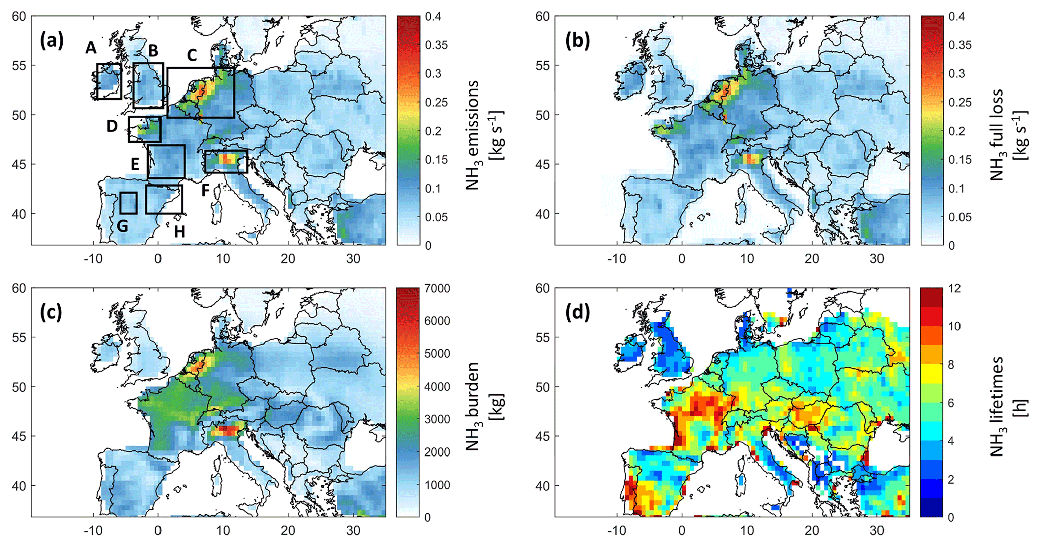
Figure 2Ammonia budget in Europe from GEOS-Chem: (a) ammonia emissions from the Harmonized Emissions Component module (HEMCO) in kilograms per second with our regions of interest shown with rectangles, (b) full ammonia loss in kilograms per second, (c) total ammonia burden in kilograms, and (d) ammonia lifetime in hours. All plots refer to March 2011 and are presented at a 0.5∘ × 0.625∘ grid resolution.
3.1 Ammonia emissions, losses, and lifetime in Europe
In order to understand the NH3 spatial variability in Europe during the application of fertilizers, a detailed analysis of the output of the GEOS-Chem simulation for the month of March 2011 is shown in Fig. 2.
The anthropogenic sources (i.e., mainly agriculture) constitute 83 % of the total ammonia emissions in March 2011 in Europe. The ammonia emissions from natural sources (i.e., soil of natural vegetation, oceans, and wild animals) follow, representing 16 % of the total emissions, whereas the remaining 1 % correspond to the ammonia emissions from biomass burning and ships (not shown here).
Figure 2a shows the monthly emissions of ammonia. Most of these emissions are due to agricultural activities (not shown here); we identify eight source regions, which we investigate thoroughly in this study, shown as rectangles A to H. The agricultural sources with the highest contribution are located in the North European Plain, Brittany, and the Po Valley (regions C, D, and F).
In the calculation of the total loss of ammonia (Fig. 2b), we considered dry deposition, chemistry, transport, and wet deposition (in which we included ammonia loss to convection) from the GEOS-Chem model simulation, which are all possible loss processes for ammonia (David et al., 2009). Figure 2b shows that the largest losses occur logically where we have the highest sources detected (see Fig. 2a).
The total ammonia burden (Fig. 2c) is calculated as the integrated sum of all ammonia columns in the model grid box. We can clearly detect ammonia hotspots over Europe, in particular the North European Plain, Brittany, and the Po Valley; all these regions are characterized by intense agricultural activities, as the total emissions and deposition show (Figs. 1 and 2). We also see that the burden is generally the highest over France, Belgium, the Netherlands, and parts of Germany and Italy.
The lifetime τss of ammonia is shown in Fig. 2d. In the case of a gas with a short lifetime, such as ammonia, the emissions are relatively well balanced spatially by eventual sinks/losses (steady-state approximation). Therefore, we can calculate a steady-state lifetime as the ratio between the total burden B (Fig. 2c) and the total emissions E or losses L (sum of all emitted/lost molecules; Fig. 2a and b) using the following equation: (Plumb and Stolarski, 2013).
We note that the τss is more or less the same whether we calculate it using the losses or the emissions. For instance, in selected source regions (rectangles in Fig. 2a) the total emissions and losses are very close, with very low biases that are less than 2 % (not shown here). Our results show that τss, on average monthly, can go up to 12 h, and it can reach 1 d (24 h) in coastal regions such as region E in New Aquitaine in France. The latter can be related to the high probability of air stagnation in that area, especially during spring, in comparison to northern Europe (Garrido-Perez et al., 2018), since higher PM2.5 pollution episodes were found under stagnant meteorological conditions (AQEG, 2012), and these PM2.5 particles can dissociate, releasing ammonia. Our results agree with the literature suggesting a residence time between a few hours and a few days (Behera et al., 2013; Pinder et al., 2008). We note that Evangeliou et al. (2021) estimated the lifetime of ammonia over Europe using a different model, and the results showed a monthly average ranging from 10 to 13 h. The figure adapted from Evangeliou et al. (2021) is shown in Fig. S1 in the Supplement. Shorter lifetimes from industrial sources of ammonia were reported in Dammers et al. (2019), with a mean lifetime of ammonia that is equal to 2.35 h (± 1.16). A recent study found lifetimes of ammonia that vary between 5 and 25 h, roughly, in Europe (Luo et al., 2022); these values are higher since, in addition to ammonia loss, Luo et al. (2022) included the loss of ammonium and thus considered the loss of ammonia to be terminal only when the ammonium is also lost/deposited. This approach is not adopted here nor in Evangeliou et al. (2021).
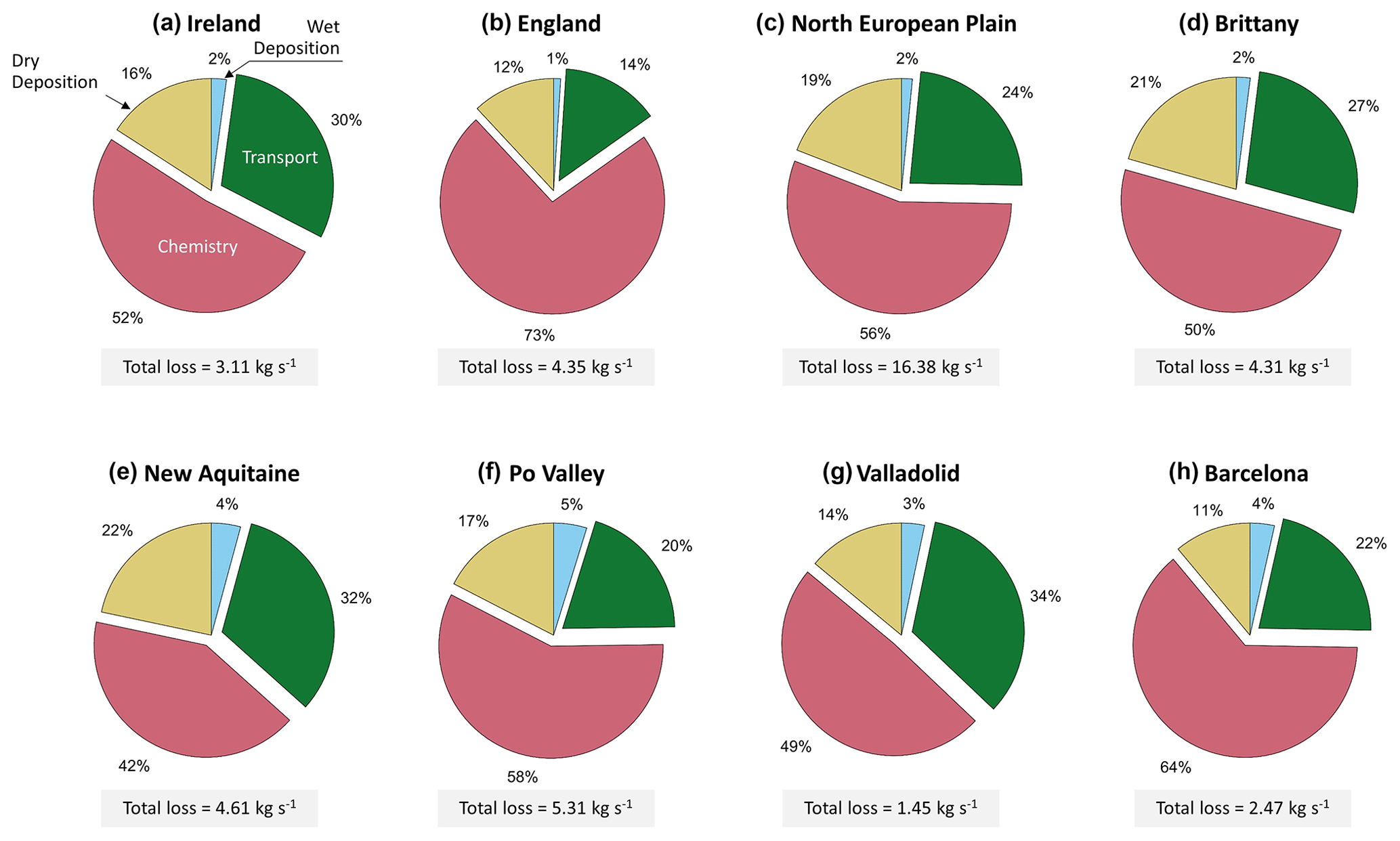
Figure 3Repartition of the ammonia loss mechanisms for major agricultural areas in Europe in March 2011, as retrieved from GEOS-Chem, with the total ammonia loss shown in the gray boxes under each pie chart (kg s−1). The regions are shown with black boxes in Fig. 2a.
Notably, ammonia lifetime and burden (Fig. 2c and d) each have a different spatial distribution compared to the other two panels (Fig. 2a and b). The ammonia residence time in the atmosphere varies depending on the sources and more importantly on the locally dominant loss mechanisms. For this reason, in Fig. 3, we show the relative contribution of the ammonia loss mechanisms, presented as pie charts, for the agricultural source regions shown by black boxes in Fig. 2a.
The fastest loss mechanisms are either chemical (i.e., in the vast majority transformation to particulate matter) or through wet and dry deposition (Tournadre et al., 2020). Figure 3 shows that more than 50 % of the ammonia molecules in the atmosphere are lost to chemical reactions in most of the regions (A, B, C, H, and F). The shortest residence time of ammonia is observed in England, where the chemical removal was significantly higher than other sinks and represented up to 73 % of the total ammonia loss pathways, suggesting a rapid transformation into inorganic particulate matter (PM2.5). In the regions D, G, and E the chemical loss makes up 50 %, 49 %, and 42 %, respectively. In fact, in March 2011, PM was found to be mostly composed of inorganic nitrate (41 %) and ammonium (20 %) (Viatte et al., 2022) over Europe, both of which are products of atmospheric ammonia. For instance, nitrate-bearing PM2.5 is formed when nitric acid (HNO3) reacts with ammonia (Yang et al., 2022), while ammonium is a direct product of the hydrolysis of ammonia. A total of 41 % of the nitric acid formed in the atmosphere is produced from the reaction between nitrogen dioxide (NO2) and the hydroxyl radical (OH) (Alexander et al., 2020). These chemical pathways help explain the large chemical losses in most of the regions studied in Fig. 3.
Ammonia loss to transport is the highest in regions neighboring the Atlantic Ocean, accounting for 30 %, 27 %, 32 %, and 34 % of total sinks in regions A, D, E, and G, respectively. These regions are exposed to the North Atlantic Drift, also known as the Gulf Stream, which is associated with high wind speed and cyclonic activity (Barnes et al., 2022). Although the Gulf Stream also affects the loss to transport in England (region B), the chemical loss is the dominant one. Acids, such as HNO3 and H2SO4, react with ammonia in the atmosphere. Therefore, high atmospheric concentrations of NO2 and SO2 (from which HNO3 and H2SO4 are derived, respectively) induce higher loss of ammonia to chemical reactions. In England, the annual concentration means of both NO2 and SO2 are higher than in Ireland (European Environment Agency, 2017a, b). This can explain why the largest proportion of NH3 is lost to chemistry in England, in spite of the effect of the Gulf Stream. In other regions, 14 % to 22 % of the total ammonia is lost to transport mechanisms, and in all regions, 11 % to 22 % is lost to dry deposition (Fig. 3).
In March, precipitation is relatively lower as compared to winter (December, January, February) in Europe. Furthermore, 2011 was a particularly dry year compared to the 1981–2010 average (Met Office, 2016). Drought was reported to be severe in areas such as France, Belgium, and the Netherlands and moderate in England and Ireland (EDO, 2011). This can help explain the low percentage of wet deposition in March 2011 (1 % to 5 % out of the total loss of ammonia).
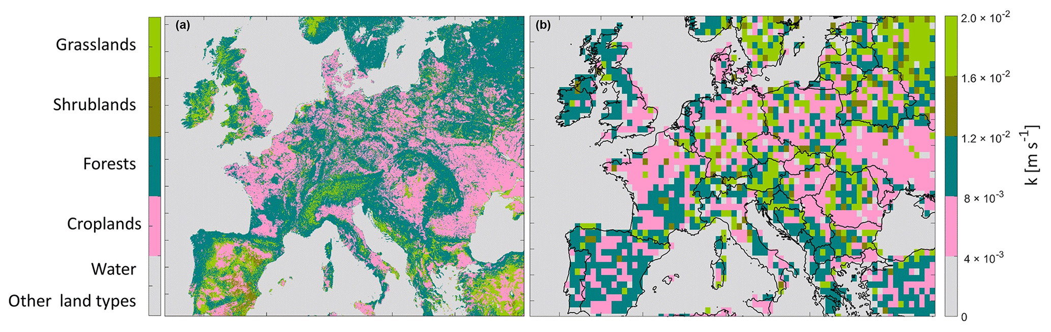
Figure 4MODIS land cover type at a 500 m × 500 m grid box resolution (a) and aggregated mass transfer coefficient k (variable k) at a horizontal grid box resolution of 0.5∘ × 0.625∘ (b).
3.2 Ammonia emission potential over Europe
To calculate emission potential, a calculation of the mass transfer coefficient k, which relates to the land type, is necessary. Figure 4 shows the land cover type from MODIS in Europe (Fig. 4a), and the corresponding assigned mass transfer coefficient k (Fig. 4b) needed to calculate the emission potential (Eq. 1). In order to choose a mass transfer coefficient that is convenient for the different land types relevant to this study, we searched for k values in the literature. Note that ammonia transfer coefficients are not available for all land types.
For waterbodies and other land types that are not considered here (see Sect. 2.2), the mass transfer values k were set to zero and are represented in gray in Fig. 4. In a laboratory experiment, Svensson and Ferm (1993) reported k = 4.3 × 10⁻³ m s−1 for a mixture of soil and swine manure; therefore, this value was assigned to croplands. Due to the lack of NH3 k values for non-fertilized forests, shrublands, and grasslands in the literature, we used values originally assigned to SO2, bearing in mind that these are approximate values, and they mostly reflect the conditions of the soil cover type (short, medium, or tall grass) rather than the gas itself. In Aneja et al. (1986), the authors estimated the mass transfer coefficient for both NH3 and SO2 above different types of crops; they found similar values. For NH3, k varied between 0.3 and 1.3 cm s−1, and for SO2 it varied between 0.5 and 1.5 cm s−1 (Aneja et al., 1986). Since the latter study estimates several values for NH3 mass transfer coefficient, over different types of crops, we use the k provided by Svensson and Ferm (1993) since it is better adapted to reflect NH3 emission from fertilizers and is not dependent on the crop type. To assign a k value for forests, we used values reported in Aneja et al. (1986) (k = 2 × 10⁻² m s−1), which originally represent deposition velocity (mass transfer) of SO2 in a forest (high crops), since both SO2 and NH3 showed similar k values above crops. For shrublands and grasslands (the two land types have the same k), we used the value k = 8 × 10⁻³ m s−1 reported in Aneja et al. (1986) as the deposition velocity (mass transfer) of SO2 in a grassland (medium crops). These values obtained by using MODIS land cover types and published estimates of k values represent our best effort to compute realistic mass transfer coefficients and therefore realistic soil emission potentials.
After choosing the k values, we assigned them for each land type on the 500 m × 500 m grid. We then aggregated the array with the k values from 500 m × 500 m to the resolution of GEOS-Chem (0.5∘ × 0.625∘ grid box). This leads to averaging different fine pixels with different land cover types into a coarser grid. The result is shown in the right panel of Fig. 4.
Uncertainties in this methodological approach can be summarized as follows:
-
The k value assigned for croplands is approximate and therefore not the same in every cropland over Europe.
-
The k value assigned for forests represents the SO2 exchange in high croplands; this value may be different for ammonia, since NH3 can easily dissolve in the water film on leaves under conditions of high humidity.
-
While changing the resolution of a fine array (500 m × 500 m), several grid points are merged and averaged together in order to construct the coarser grid box (0.5∘ × 0.625∘ ); the result is therefore an average that might mix croplands with neighboring forests/bare lands/grasslands. This leads to a range of different k values that are shown in Fig. 4.
Using a land-type-specific k value is necessary in order to reflect realistic emission potential; we call this the variable k, as ammonia exchange in a forest is different from that of croplands or unfertilized grasslands due to different barriers (long, medium, or short crop/grass) and ammonium soil content in each land type.
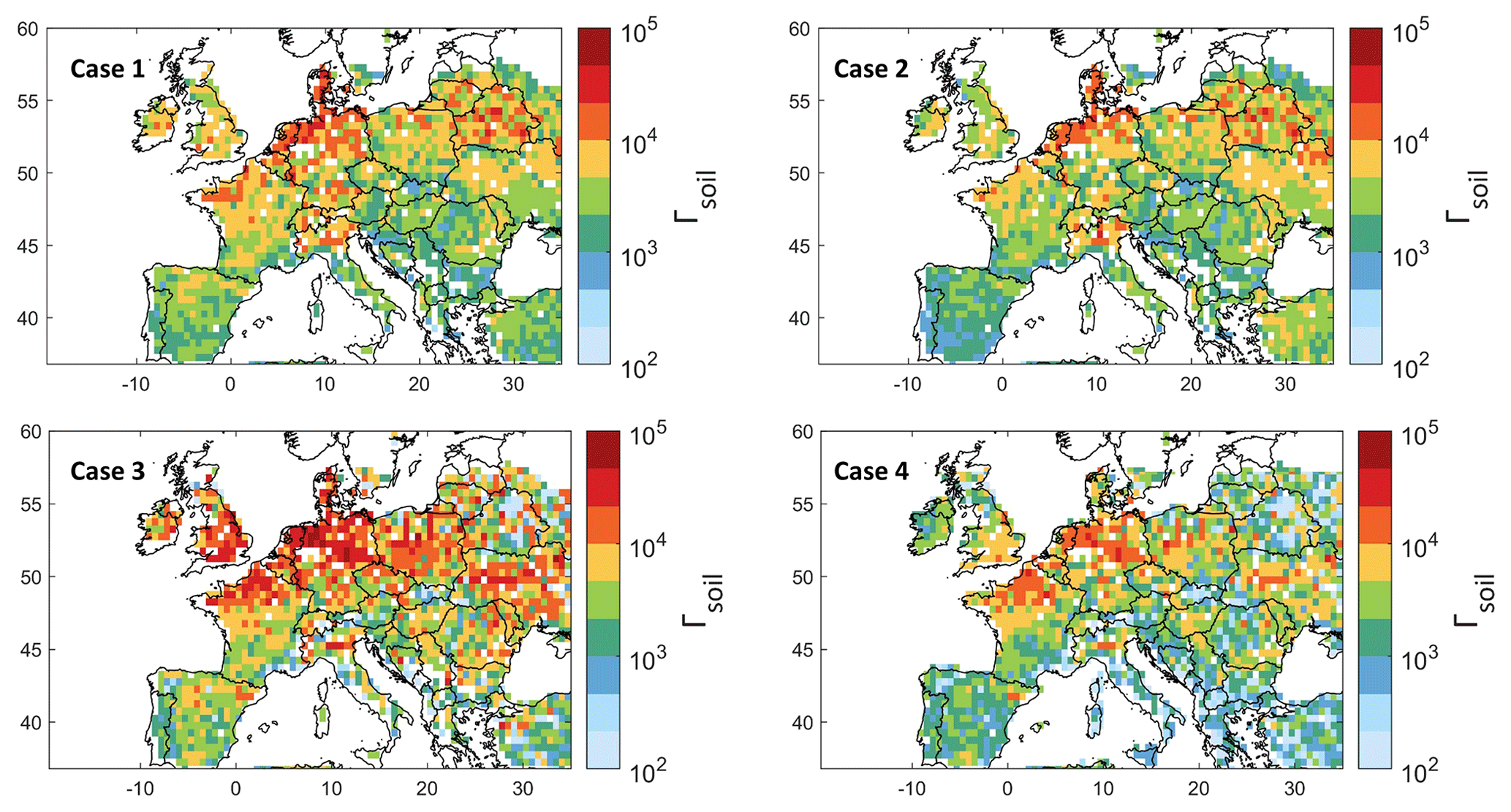
Figure 5Ammonia soil emission potential (Γsoil) on a log10 scale from model simulation, observation, and reanalysis for four different cases (see text for details).
Figure 5 illustrates the ammonia soil emission potential Γsoil calculated using Eq. (1) and k values presented in Fig. 4. After assigning a variable mass transfer coefficient, the remaining variables needed to calculate Γsoil in Eq. (1) are ammonia concentration and lifetime, as well as the skin temperature. Therefore, the emission potential Γsoil shown in Fig. 5 is calculated using different configurations.
-
Case 1: GEOS-Chem ammonia and lifetime and MERRA-2 Tskin, i.e., simulated Γsoil;
-
Case 2: GEOS-Chem ammonia and lifetime and ERA5 Tskin to check the effect of using ERA5 vs. MERRA-2 for skin temperature;
-
Case 3: IASI ammonia, ERA5 Tskin, and GEOS-Chem ammonia lifetime;
-
Case 4: IASI ammonia, ERA5 Tskin, and ammonia lifetime from Evangeliou et al. (2021), calculated using the LMDz-OR-INCA chemistry transport model (the latter couples three models – the general circulation model GCM (LMDz) (Hourdin et al., 2006), the INteraction with Chemistry and Aerosols (INCA) (Folberth et al., 2006), and the land surface dynamical vegetation model (ORCHIDEE) (Krinner et al., 2005)).
We show in Fig. S2 the emission potential (similarly to what we show in Fig. 5), but from a fixed and averaged k value for all land types. Figure S2 shows the importance of using a variable k that is adjusted to each land type. To calculate a fixed k (common to all land types) we assume 14 d of fertilization (k = 10−3 m s−1, e.g., croplands), 7 d when the k value is reduced (k = 10−5 m s−1), and 10 d when k is low (k = 10−6 m s−1, e.g., forests), resulting in an average of k = 4.5 × 10⁻⁴ m s−1. The difference in the emission potential between fixed and spatially variable k is shown in Fig. S3, where we see that a fixed k might overestimate Γsoil by 10 to 103 on a log10 scale (500 %–3000 %) in agricultural areas.
When calculating Γsoil, we filtered data points with ammonia total column concentration less than 5 × 10¹⁴ . The latter are mostly grid boxes concentrated above 56∘ north that we consider to be noise (shown with white pixels in Fig. 5).
Tskin from ERA5 and MERRA-2 agree very well, with a coefficient of determination r2 = 0.97 (Fig. S4). This explains the excellent spatial correlation between cases 1 and 2. Note that when using MERRA-2 Tskin, we selected only morning measurements from 08:00 to 10:00 UTC. Since IASI NH3 retrievals use ERA5 Tskin, this also suggests that using MERRA-2 or ERA5 does not affect our Γsoil calculation. In case 3, the emission potential agrees spatially with that of GEOS-Chem. However, we observe higher Γsoil in regions such as Ireland, England, northern France, northeastern Spain, and Poland. This is due to the underestimation of ammonia from GEOS-Chem as compared to IASI observations (Fig. 1a). For instance, Γsoil from IASI and ERA5 (case 3) differs from that from GEOS-chem and ERA5 (case 1) by 31 % in Ireland. Looking at Table 1, this difference can be explained by the corresponding MRD for Ireland (−45 %). The differences between case 3 and 4 reach up to +72 % in Ireland, and this is mostly due to the 10 h difference between ammonia lifetime from GEOS-Chem and Evangeliou et al. (2021) (Fig. S1). The lowest Γsoil values (in most regions) were obtained in case 4, due to the higher lifetime values from Evangeliou et al. (2021), as compared to those calculated from GEOS-Chem (Fig. S1); note that Γsoil is inversely proportional to ammonia lifetime (Eq. 1). In fact, the longer ammonia stays in the atmosphere (longer lifetime), the less the flux will be directed from the soil to the atmosphere (less ammonia emission). We compared Γsoil calculated from all cases for each region, and we conclude that cases 2 and 4 showed the best compatibility. For instance, Γsoil values from cases 2 and 4 differ by only 6 % in the North European Plain and Brittany and by 4 % in New Aquitaine. The highest difference between cases 2 and 4 is observed in the Po Valley (53 %) (not shown here).
In the four cases presented in Fig. 5, we see similar spatial distribution of ammonia emission potential, with values ranging from 12 × 10−1 in a forest to 9.5 × 10⁴ in a cropland (monthly average considering all the cases). In agricultural lands, our results show that Γsoil ranges from 2 × 10³ to 9.5 × 10⁴. In fact, most of the studies summarized in Zhang et al. (2010) reported Γsoil values that range mostly from 103 to 104 in fertilized croplands/grasslands; the minimum Γsoil reported is on the order of 102, and the maximum is of the order of 105. Therefore, our values fit within the range of Γsoil calculated in the literature and summarized in Zhang et al. (2010) and the references within. Personne et al. (2015) focused on Grignon, an agricultural region near Paris, France (48∘51′ N, 01∘58′ E). They obtained Γsoil values between 1.1 × 10⁴ and 5.8 × 10⁶. In the present study, the emission potential over this region is between 4 × 10³ (case 2) and 5 × 10³ (case 4). In this study, lower values than those measured in the field are expected. Therefore, we consider our results to be in good agreement with the values in Personne et al. (2015), since ours reflect a 31 d mean of an average of Γsoil over a large area (55 × 70 km2) as compared to the localized measurements done by Personne et al. (2015).
The mean emission potentials per ammonia source region in Europe (shown with rectangles in Figs. 2 and 3) and per case are shown in Fig. 6 and listed in Table 1. Table 1 shows the average lifetime from GEOS-Chem (hours), the average Tskin from the two datasets that we used (∘C), the average ammonia emission potential in all the cases examined (dimensionless), and the average ammonia columns from IASI and GEOS-Chem (). The four cases show a similar pattern, with the North European Plain exhibiting the highest emission potential. This is shown in Figs. 1, 2, and 5, as well as in Table 1, where Γsoil is higher in regions with high ammonia columns. This is expected in fertilized lands (croplands), since Γsoil is proportional to the concentration of ammonia near the surface. The latter increases when the soil content of ammonium () increases following the application of nitrogen-based fertilizers.
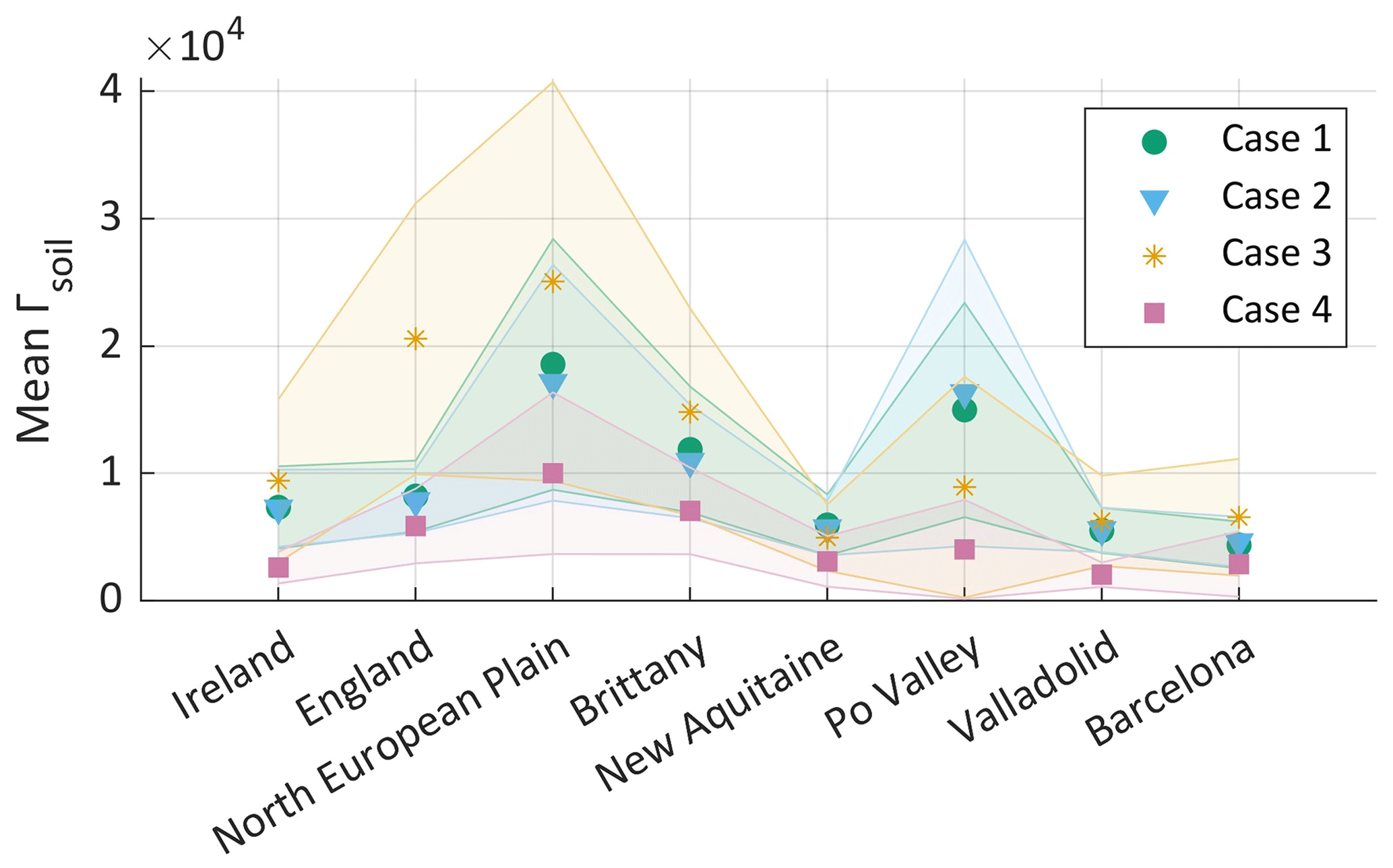
Figure 6Mean ammonia emission potential Γsoil per region and per case, with the error margin of the mean as the shaded area (95th percentile) for cases 1 to 4. The cases are explained in the discussion of Fig. 5.
Figure 6 also shows that for cases 1 and 2 (GEOS-Chem) the emission potential in the Po Valley is almost equal to case 3 (IASI), with Γsoil = 0.9 and 0.86 × 10⁴ in cases 1 and 2 and 0.89 × 10⁴ in case 3 (see Table 1). To calculate Γsoil from IASI NH3 (case 3 and 4), we used Tskin from ERA5 that coincides with the overpass of IASI. We used the same Tskin values from ERA5 for case 2, as well as hourly concentrations of ammonia from GEOS-Chem (08:30 to 11:30 UTC). The ERA5 Tskin values are shown in Table 1. The effect of skin temperature through Eq. (1) makes the emission potential highly dependent on it. In fact, Γsoil is both directly and inversely proportional to Tskin; however, the exponential in the denominator has an effect on the value of Γsoil that is ∼ 10 times greater than the Tskin in the numerator. Therefore, through Eq. (1), we conclude that an increase in temperature by 1 ∘C will reduce Γsoil by around −8 %.
The standard deviation (shaded area) is found to be the highest in the North European Plain, which is also the largest region (hence higher variability is expected), especially when considering case 3 with IASI. IASI distinguishes different source sub-regions, leading to higher spatial variability in ammonia and therefore Γsoil.
3.3 The effect of temperature change on the volatilization of ammonia
As seen in Eq. (1), higher skin temperatures favor volatilization of ammonia from the soil. In an attempt to understand how our simplified emission potential model behaves under changing climate, as well as under future scenarios, we adopt the future Tskin simulations from the EC-Earth climate model in Eq. (1). The two socio-economic climate scenarios that we consider are SSP2-4.5 (middle-of-the-road scenario, where trends broadly follow their historical patterns) and SSP5-8.5 (a world of rapid and unconstrained growth in economic output and energy use) (Riahi et al., 2017). The same figure constructed using Γsoil from GEOS-Chem (case 1) is shown in Fig. S5 in the Supplement.
We calculate current and future ammonia columns assuming that the emission potential Γsoil remains unchanged. In other words, we assume that the same quantity of fertilizers and manure is used until 2100 in the agricultural fields and farms (unchanged ammonium soil content).
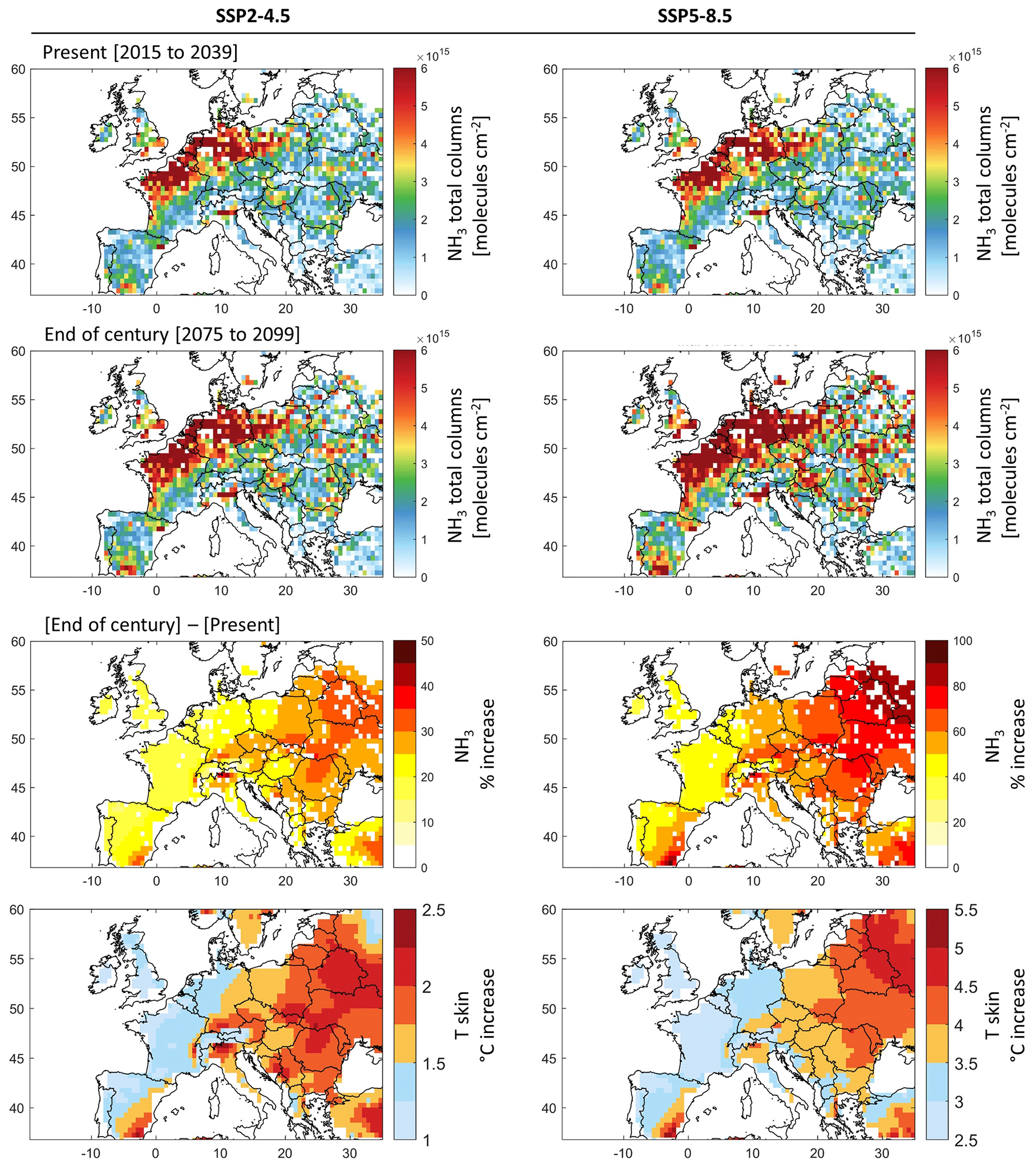
Figure 7First and second rows: ammonia total column concentrations in March (monthly averages) under the present climate (2015 to 2039; first row) and the end-of-the-century climate (2075 to 2099; second row) under the socio-economic scenarios SSP2-4.5 (left) and SSP5-8.5 (right). Third and fourth rows: the percentage increase in ammonia concentration (third row) and the change in Tskin in degrees Celsius (fourth row) by the end of the century (2075 to 2099) with respect to present climate (2015 to 2039) under SSP2-4.5 (left) and SSP5-8.5 (right). Ammonia columns were calculated using ammonia emission potential Γsoil derived from IASI and ERA5 for March 2011 (case 3) and EC-Earth Tskin simulations for SSP2-4.5 and SSP5-8.5 extending from 2015 till 2099.
Figure 7 shows ammonia columns during the 25 years (2015–2039) representing the present climate (upper panels) and the end of the century (2075–2099; middle panels). The ammonia columns in the 25-year average climate of the end of the century with respect to present-day climate (lower panels) are also shown.
Spatially, the present-climate ammonia columns calculated from the Tskin of the climate model and our emission potential from IASI (case 3 in Fig. 5) agree very well with those shown in Fig. 1. We do not aim at validating or directly comparing the two, as we are only interested in the climate response to ammonia concentration, i.e., by the difference due to skin temperature increase (lower panels).
From Fig. 7 (lower panels) it can be seen that the increase in ammonia columns by the end of the century is more severe in eastern Europe. Under the most likely scenario (SSP2-4.5), ammonia columns vary between +15 % in France and around +20 % in the North European Plain (Fig. 7). The largest increase is detected in eastern Europe, where ammonia columns show an increase of up to +50 % (Fig. 7, lower left panels), creating new potential hotspots/sources of ammonia in Belarus, Ukraine, Hungary, Moldova, parts of Romania, and Switzerland. Under the SSP5-8.5 scenario, the results show an increase in ammonia columns of up to +100 % in eastern Europe (Fig. 7, lower right panel). This is directly related to the higher projected increase in skin temperature over these regions. Other studies have equally reported eastern Europe to be more affected by climate change under future scenarios, as compared to western Europe (European Environment Agency, 2022; Jacob et al., 2018). Spatially, the increase in ammonia coincides with the increase in Tskin.
Figure 8 depicts the change in ammonia columns under the SSP2-4.5 and SSP5-8.5 scenarios for our source regions (shown as rectangles in Fig. 2). Ammonia column increase is foreseen to be the highest in the Po Valley (Italy), with +26 % and +59 % under SSP2-4.5 and SSP5-8.5, respectively. It is then followed by the agricultural areas around Barcelona (Spain) and the North European Plain (Belgium, the Netherlands), with an increase of +21 % (+49 %) and +20 % (+53 %), respectively, under the SSP2-4.5 (SSP5-8.5) scenario. Under SSP5-8.5, the increase in ammonia columns in percentage is more than twice the change under SSP2-4.5 (+127 % in the case of the Po Valley for instance). The Po Valley is adjacent to the Alps, and due to global warming, this region is expected to experience increased evapotranspiration (Donnelly et al., 2017), which is a major factor that leads to the volatilization of ammonia.
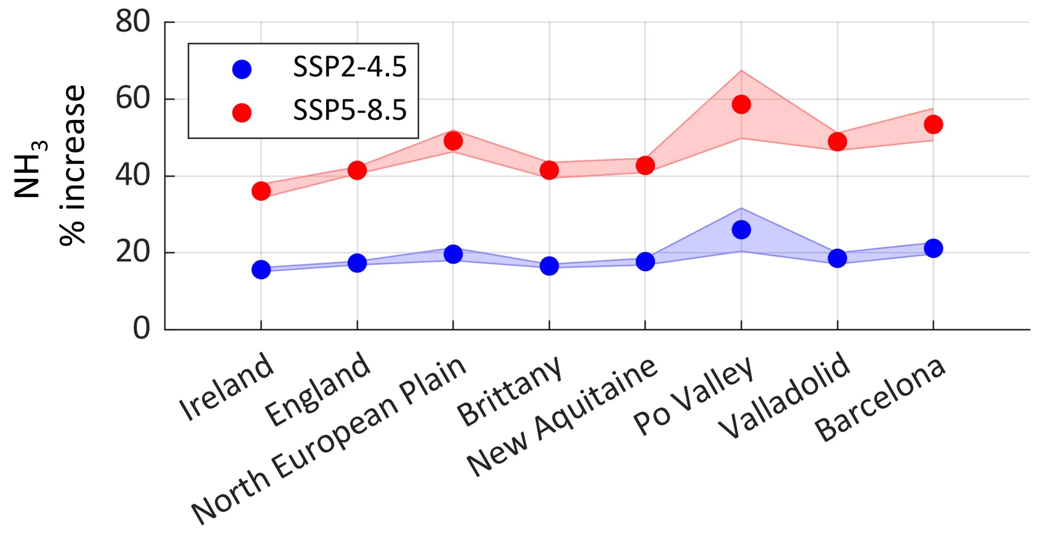
Figure 8The percentage increase in ammonia concentration by the end of the century (2075 to 2099) with respect to the present climate (2015 to 2039) under the two climate scenarios SSP2-4.5 (blue) and SSP5-8.5 (red) in the source regions investigated in this study. The shades around each line represent the standard deviation from the mean.
The local and regional effect of volatilization of ammonia under different climate scenarios remains difficult to properly assess. Even under the middle-of-the-road scenario SSP2-4.5, and without climate extremes (e.g., heat waves), Europe might be facing big challenges in air quality for regions nearby or downwind agricultural regions, since chemistry and atmospheric transport (Fig. 3) drive the loss of ammonia during the growing season in this part of the world.
An increase in ammonia concentration has a significant and yet poorly understood effect on local and regional air quality through the increase in PM2.5 concentration. We note, however, that ammonia columns in the soil are governed by a threshold. Higher temperatures will increase the rate of volatilization of ammonia from the soil, but only up to a certain point where no dissolved ammonium is left. Plants, however, can also be a source of ammonia when exposed to stressful conditions. For example, under heat stress and in instances where there is no ammonia in the air, an increase in air temperature results in an exponential increase in ammonia emission from plants' leaves (Husted and Schjoerring, 1996).
Agriculture worldwide has fed the human race for thousands of years and will continue to do so, as humankind highly relies on it. Emissions from agricultural activities will inevitably increase in order to meet the expected yield. In this study, we use a variety of state-of-the-art datasets (satellite, reanalysis, and model simulation) to calculate the first regional map of ammonia emission potential during the start of the growing season in Europe. The emission potential can be used as a proxy to calculate ammonia columns in the atmosphere and as such to assess its deposition, atmospheric transport, and contribution to PM formation. First, we show that the GEOS-Chem chemistry transport model is able to reproduce key spatio-temporal patterns of ammonia levels over Europe. The ammonia budget is governed by the emissions over source regions (North European Plain, Brittany, and the Po Valley), as well as by key loss processes. We find that the chemical loss pathway is responsible for 50 % or more of the total ammonia loss over Europe. From the GEOS-Chem simulation, we calculate the average ammonia lifetime in the atmosphere, which ranges between 4 and 12 h in agricultural source regions of Europe. From this, and using the mass transfer coefficient for different land cover types, we calculate a range of emission potentials Γsoil from IASI and GEOS-Chem. We find that Γsoil ranges from 0.2 × 10⁴ to 2.5 × 10⁴ in fertilized lands (croplands). Choosing a variable k from the literature, and based on different land cover types from MODIS, we calculate Γsoil values that are consistent with those found in the literature. The increase in Tskin is expected to have an effect on the emission of ammonia from the soil. Using Tskin from the EC-Earth climate model, we estimate ammonia columns by the end of the century (2075–2099) and compare them to columns of the present climate (2015–2039). Our results show that ammonia columns might double under the SSP5-8.5 scenario and might increase by up to 50 % under the most likely SSP2-4.5 scenario. The eastern part of Europe is the most affected by the change in temperatures, and it is where we find the highest ammonia column increase. Among the regions of focus, Italy, Spain, Belgium, and the Netherlands are the most affected, as compared to France, England, and Ireland. The highest increase in ammonia columns is observed in the Po Valley in Italy (+59 % under the SSP5-8.5).
We calculate ammonia concentration under future climate and during the start of the growing season (March) in Europe. However, in order to grasp the yearly budget of ammonia, it is crucial to apply this method to all seasons of the year, especially in regions with extensive agricultural activities, such as the United States, India, and China. In addition to this, more field measurements of ammonia emission potential (Γsoil) in different land use/cover types are required; this can help us perform better comparison with emission potentials calculated from model and satellite data. Finally, having ammonia columns at different times of the day from field observations or satellite measurements will allow quantification of daily emission potentials, which will in turn help us understand its diurnal variability. This will be ensured with the launch of the Infrared Sounder (IRS) on the Meteosat Third Generation (MTG) geostationary satellites scheduled in 2025.
A1 Ammonia–ammonium equilibrium
Ammonia (NH3) is a water-soluble gas; it undergoes protonation with H+ from the hydronium ion H3O+ in an aqueous solution in order to give ammonium ( cation). The dissociation equation is expressed as follows:
or
with as the ammonium–ammonia dissociation equilibrium constant, that can be expressed as
The solubility of ammonia in water is affected by the temperature and the acidity (pH) of the solvent (water). The equilibrium constant can be expressed as follows:
A2 Henry's equilibrium
Upon its dissolution in water, NH3 obeys Henry's law. Ammonia gas (NH3 (g)) near the surface of the solvent is in equilibrium with the dissolved ammonia in the aqueous-phase NH3 (aq) (in water). Henry's equilibrium is expressed as follows:
where is Henry's constant, which can be expressed as (Wichink Kruit, 2010)
The partial pressure of ammonia near the surface of the soil can be calculated using Henry's constant and the dissociation equilibrium (Wichink Kruit, 2010):
If we use the ideal gas law (PV = nRT), we can draw a link between the mass density of ammonia (NH3 (g)) and the partial pressure:
where is the concentration of NH3 at the soil surface (kg m−3), is the partial pressure of NH3 near the surface (atm), is the molar mass of NH3 (kg mol−1), R is the gas constant (0.082 ), and T is the temperature in Kelvin.
Substituting Eq. (A7) into (A8) we get
where is the concentration of ammonia at the soil surface at equilibrium (g m−3) and is referred to as the compensation point, Tsoil is the temperature of the soil (Kelvin), and is the NH3 emission potential from the soil and is a dimensionless ratio between [] and [H+].
A3 Ammonia total columns from IASI
In this study we use the total columns of ammonia from IASI () since in order to calculate the emission potential Γsoil, we should draw a link between these columns and this parameter. The bidirectional exchange of NH3 between the surface and the atmosphere can be expressed by the flux (assuming a flux independent of time) (Roelle and Aneja, 2005; Zhang et al., 2010):
where is the bidirectional flux between the soil and the atmosphere (); k is the soil–atmosphere exchange velocity (m s−1), also known as the mass transfer coefficient; [NH3]soil is the concentration of NH3 (g) in the soil; and [NH3]atm is the concentration of NH3 (g) in the atmosphere near the surface (). We can consider that [NH3]atm is identical to the total column of NH3 provided by IASI and denoted here as [NH3]col. This is because most of the atmospheric NH3 is located in the lower boundary layer (Dammers et al., 2019). Assuming a first-order dissociation of NH3, we can express the change in the [NH3]col total columns as follows:
where k′ is the rate of dissociation of first-order (m s−1), with τ the lifetime of NH3 in the atmosphere. Assuming steady state, and considering the [NH3]atm to be the [NH3]col and [NH3]soil to be , Eq. (A11) can be written as
where c is the column height and is equal to 6 km. It is important to note that we neglect the effect of transport by wind since we only look at large regions. Finally, the total column of ammonia [NH3]col can be written as
The column height is not considered anymore because it is negligible compared to . Using Eq. (A9) in Eq. (A13) we get
Note that 9.72 × 1023 = ((K molec.) (s cm2)−1), where a = 2.75 × 10³ (g K cm−3), Na is Avogadro's number (6.0221409 × 10²³ ), c′ = 10−2 is added to convert k from meters per second to centimeters per second, and is the molar mass of NH3 (17.031 g mol−1). The emission potential of NH3 from the soil can be written as
where b = 1.04 × 10⁴ K.
The IASI NH3 data used in this study are retrieved from the Aeris data infrastructure (https://iasi.aeris-data.fr/nh3r-era5/, LATMOS-ULB, 2023). ERA5 skin temperature from 1979 to present is available for download from the following DOI: https://doi.org/10.24381/cds.adbb2d47 (Hersbach et al., 2023). The GEOS-Chem outputs used in this study are only available upon request. EC-Earth3 model output prepared for CMIP6 ScenarioMIP is retrieved here: https://doi.org/10.22033/ESGF/CMIP6.727 (EC-Earth Consortium, 2019). The MODIS land cover data are available for download from the following link: https://doi.org/10.5067/MODIS/MCD12Q1.006 (Friedl and Sulla-Menashe, 2019).
The supplement related to this article is available online at: https://doi.org/10.5194/acp-23-12505-2023-supplement.
RA contributed to the conception and design of the article, developed the code, wrote the manuscript, analyzed and interpreted the data, and approved the version for submission; CV, CC, and PFC revised the manuscript; WCP provided the GEOS-Chem simulation data and revised the manuscript; NE provided ammonia lifetime calculation using the LMDz-OR-INCA chemistry transport model and commented on the manuscript; MVD and LC contributed to the acquisition of the IASI ammonia data (NH3-v3R-ERA5) and revised the manuscript; SS contributed to the conception and design of the article, provided the EC-Earth temperature data, revised the manuscript, and approved the version for submission.
The contact author has declared that none of the authors has any competing interests.
Publisher's note: Copernicus Publications remains neutral with regard to jurisdictional claims in published maps and institutional affiliations.
The IASI mission is a joint mission of EUMETSAT and the Centre National d'Etudes Spatiales (CNES, France). The authors acknowledge the Aeris data infrastructure for providing the IASI L1C and L2 data.
Rimal Abeed received financial support from CNES. The research in Belgium was funded by the Belgian State Federal Office for Scientific, Technical and Cultural Affairs (Prodex HIRS) and the Air Liquide Foundation (TAPIR project). This work is also partly supported by the FED-tWIN project ARENBERG (“Assessing the Reactive Nitrogen Budget and Emissions at Regional and Global Scales”), funded via the Belgian Science Policy Office (BELSPO). Lieven Clarisse is a research associate and is supported by the Belgian F.R.S.-FNRS. Cathy Clerbaux received financial support from CNES. Nikolaos Evangeliou was funded by Norges Forskningsråd (ROM-FORSK – Program for romforskning of the Research Council of Norway; grant no. 275407).
This paper was edited by Amos Tai and reviewed by two anonymous referees.
Abeed, R., Clerbaux, C., Clarisse, L., Van Damme, M., Coheur, P.-F., and Safieddine, S.: A space view of agricultural and industrial changes during the Syrian civil war, Elem. Sci. Anthr., 9, 000041, https://doi.org/10.1525/elementa.2021.000041, 2021.
Adams, C., McLinden, C. A., Shephard, M. W., Dickson, N., Dammers, E., Chen, J., Makar, P., Cady-Pereira, K. E., Tam, N., Kharol, S. K., Lamsal, L. N., and Krotkov, N. A.: Satellite-derived emissions of carbon monoxide, ammonia, and nitrogen dioxide from the 2016 Horse River wildfire in the Fort McMurray area, Atmos. Chem. Phys., 19, 2577–2599, https://doi.org/10.5194/acp-19-2577-2019, 2019.
Alexander, B., Sherwen, T., Holmes, C. D., Fisher, J. A., Chen, Q., Evans, M. J., and Kasibhatla, P.: Global inorganic nitrate production mechanisms: comparison of a global model with nitrate isotope observations, Atmos. Chem. Phys., 20, 3859–3877, https://doi.org/10.5194/acp-20-3859-2020, 2020.
Aneja, V. P., Rogers, H. H., and Stahel, E. P.: Dry Deposition of Ammonia at Environmental Concentrations on Selected Plant Species, J. Air Pollut. Control Assoc., 36, 1338–1341, https://doi.org/10.1080/00022470.1986.10466183, 1986.
AQEG: Fine particulate matter (PM2.5) in the United Kingdom (p. 203), Air Quality Expert Group (AQEG), prepared for the Department for Environment, Food and Rural Affairs (Defra), Scottish Executive, Welsh Government and the Department of the Environment in Northern Ireland, https://uk-air.defra.gov.uk/assets/documents/reports/cat11/1212141150_AQEG_Fine_Particulate_Matter_in_the_UK.pdf (last access: 26 September 2023), 2012.
Barnes, A. P., Svensson, C., and Kjeldsen, T. R.: North Atlantic air pressure and temperature conditions associated with heavy rainfall in Great Britain, Int. J. Climatol., 42, 3190–3207, https://doi.org/10.1002/joc.7414, 2022.
Bauer, S. E., Tsigaridis, K., and Miller, R.: Significant atmospheric aerosol pollution caused by world food cultivation, Geophys. Res. Lett., 43, 5394–5400, https://doi.org/10.1002/2016GL068354, 2016.
Behera, S. N., Sharma, M., Aneja, V. P., and Balasubramanian, R.: Ammonia in the atmosphere: A review on emission sources, atmospheric chemistry and deposition on terrestrial bodies, Environ. Sci. Pollut. R., 20, 8092–8131, https://doi.org/10.1007/s11356-013-2051-9, 2013.
Belward, A. S., Estes, John E., and Kline, K. D.: The IGBP-DIS Global 1-Km Land-Cover Data Set DIS-Cover: A Project Overview, Photogramm. Eng. Rem. S., 65, 1013–1020, https://www.asprs.org/wp-content/uploads/pers/1999journal/sep/1999_sept_1013-1020.pdf (last access: 26 September 2023), 1999.
Bey, I., Jacob, D. J., Yantosca, R. M., Logan, J. A., Field, B. D., Fiore, A. M., Li, Q., Liu, H. Y., Mickley, L. J., and Schultz, M. G.: Global modeling of tropospheric chemistry with assimilated meteorology: Model description and evaluation, J. Geophys. Res.-Atmos., 106, 23073–23095, https://doi.org/10.1029/2001JD000807, 2001.
Bouwman, A. F., Lee, D. S., Asman, W. A. H., Dentener, F. J., Van Der Hoek, K. W., and Olivier, J. G. J.: A global high-resolution emission inventory for ammonia, Global Biogeochem. Cy., 11, 561–587, https://doi.org/10.1029/97GB02266, 1997.
Clarisse, L., Van Damme, M., Clerbaux, C., and Coheur, P.-F.: Tracking down global NH3 point sources with wind-adjusted superresolution, Atmos. Meas. Tech., 12, 5457–5473, https://doi.org/10.5194/amt-12-5457-2019, 2019a.
Clarisse, L., Van Damme, M., Gardner, W., Coheur, P.-F., Clerbaux, C., Whitburn, S., Hadji-Lazaro, J., and Hurtmans, D.: Atmospheric ammonia (NH3) emanations from Lake Natron's saline mudflats, Sci. Rep.-UK, 9, 4441, https://doi.org/10.1038/s41598-019-39935-3, 2019b.
Clerbaux, C., Boynard, A., Clarisse, L., George, M., Hadji-Lazaro, J., Herbin, H., Hurtmans, D., Pommier, M., Razavi, A., Turquety, S., Wespes, C., and Coheur, P.-F.: Monitoring of atmospheric composition using the thermal infrared IASI/MetOp sounder, Atmos. Chem. Phys., 9, 6041–6054, https://doi.org/10.5194/acp-9-6041-2009, 2009.
Coheur, P.-F., Clarisse, L., Turquety, S., Hurtmans, D., and Clerbaux, C.: IASI measurements of reactive trace species in biomass burning plumes, Atmos. Chem. Phys., 9, 5655–5667, https://doi.org/10.5194/acp-9-5655-2009, 2009.
Dammers, E., McLinden, C. A., Griffin, D., Shephard, M. W., Van Der Graaf, S., Lutsch, E., Schaap, M., Gainairu-Matz, Y., Fioletov, V., Van Damme, M., Whitburn, S., Clarisse, L., Cady-Pereira, K., Clerbaux, C., Coheur, P. F., and Erisman, J. W.: NH3 emissions from large point sources derived from CrIS and IASI satellite observations, Atmos. Chem. Phys., 19, 12261–12293, https://doi.org/10.5194/acp-19-12261-2019, 2019.
David, M., Loubet, B., Cellier, P., Mattsson, M., Schjoerring, J. K., Nemitz, E., Roche, R., Riedo, M., and Sutton, M. A.: Ammonia sources and sinks in an intensively managed grassland canopy, Biogeosciences, 6, 1903–1915, https://doi.org/10.5194/bg-6-1903-2009, 2009.
Donnelly, C., Greuell, W., Andersson, J., Gerten, D., Pisacane, G., Roudier, P., and Ludwig, F.: Impacts of climate change on European hydrology at 1.5, 2 and 3 degrees mean global warming above preindustrial level, Climatic Change, 143, 13–26, https://doi.org/10.1007/s10584-017-1971-7, 2017.
Döscher, R., Acosta, M., Alessandri, A., Anthoni, P., Arsouze, T., Bergman, T., Bernardello, R., Boussetta, S., Caron, L.-P., Carver, G., Castrillo, M., Catalano, F., Cvijanovic, I., Davini, P., Dekker, E., Doblas-Reyes, F. J., Docquier, D., Echevarria, P., Fladrich, U., Fuentes-Franco, R., Gröger, M., v. Hardenberg, J., Hieronymus, J., Karami, M. P., Keskinen, J.-P., Koenigk, T., Makkonen, R., Massonnet, F., Ménégoz, M., Miller, P. A., Moreno-Chamarro, E., Nieradzik, L., van Noije, T., Nolan, P., O'Donnell, D., Ollinaho, P., van den Oord, G., Ortega, P., Prims, O. T., Ramos, A., Reerink, T., Rousset, C., Ruprich-Robert, Y., Le Sager, P., Schmith, T., Schrödner, R., Serva, F., Sicardi, V., Sloth Madsen, M., Smith, B., Tian, T., Tourigny, E., Uotila, P., Vancoppenolle, M., Wang, S., Wårlind, D., Willén, U., Wyser, K., Yang, S., Yepes-Arbós, X., and Zhang, Q.: The EC-Earth3 Earth system model for the Coupled Model Intercomparison Project 6, Geosci. Model Dev., 15, 2973–3020, https://doi.org/10.5194/gmd-15-2973-2022, 2022.
EC-Earth Consortium (EC-Earth): EC-Earth-Consortium EC-Earth3-Veg model output prepared for CMIP6 ScenarioMIP, Earth System Grid Federation [data set], https://doi.org/10.22033/ESGF/CMIP6.727, 2019.
ECMWF: IFS Documentation CY43R1, ECMWF, https://www.ecmwf.int/sites/default/files/elibrary/2016/17117-part-iv-physical-processes.pdf (last access: 26 September 2023), 2016.
EDO: Drought news in Europe: Situation in April 2011—Short Analysis of data from the European Drought Observatory (EDO), p. 2, European Drought Observatory (EDO), https://edo.jrc.ec.europa.eu/documents/news/EDODroughtNews201104.pdf (last access: 26 September 2023), 2011.
Einarsson, R., Sanz-Cobena, A., Aguilera, E., Billen, G., Garnier, J., van Grinsven, H. J. M., and Lassaletta, L.: Crop production and nitrogen use in European cropland and grassland 1961–2019, Scientific Data, 8, 1, https://doi.org/10.1038/s41597-021-01061-z, 2021.
Erisman, J. W., Van Pul, A., and Wyers, P.: Parametrization of surface resistance for the quantification of atmospheric deposition of acidifying pollutants and ozone, Atmos. Environ., 28, 2595–2607, https://doi.org/10.1016/1352-2310(94)90433-2, 1994.
European Environment Agency: Nitrogen Dioxide (NO2): annual mean concentrations in Europe, https://www.eea.europa.eu/themes/air/interactive/no2 (last access: 26 September 2023), 2017a.
European Environment Agency: Sulphur Dioxide (SO2): annual mean concentrations in Europe, https://www.eea.europa.eu/themes/air/interactive/so2 (last access: 26 September 2023), 2017b.
European Environment Agency: Global and European temperatures, https://www.eea.europa.eu/ims/global-and-european-temperatures (last access: 26 September 2023), 2022.
Evangeliou, N., Balkanski, Y., Eckhardt, S., Cozic, A., Van Damme, M., Coheur, P.-F., Clarisse, L., Shephard, M. W., Cady-Pereira, K. E., and Hauglustaine, D.: 10-year satellite-constrained fluxes of ammonia improve performance of chemistry transport models, Atmos. Chem. Phys., 21, 4431–4451, https://doi.org/10.5194/acp-21-4431-2021, 2021.
Eyring, V., Bony, S., Meehl, G. A., Senior, C. A., Stevens, B., Stouffer, R. J., and Taylor, K. E.: Overview of the Coupled Model Intercomparison Project Phase 6 (CMIP6) experimental design and organization, Geosci. Model Dev., 9, 1937–1958, https://doi.org/10.5194/gmd-9-1937-2016, 2016.
FAO: FAO, GIEWS, Earth Observation, https://www.fao.org/giews/earthobservation/country/index.jsp?lang=en&code=FRA (last access: 26 September 2023), 2022.
Flechard, C. R., Spirig, C., Neftel, A., and Ammann, C.: The annual ammonia budget of fertilised cut grassland – Part 2: Seasonal variations and compensation point modeling, Biogeosciences, 7, 537–556, https://doi.org/10.5194/bg-7-537-2010, 2010.
Flechard, C. R., Nemitz, E., Smith, R. I., Fowler, D., Vermeulen, A. T., Bleeker, A., Erisman, J. W., Simpson, D., Zhang, L., Tang, Y. S., and Sutton, M. A.: Dry deposition of reactive nitrogen to European ecosystems: a comparison of inferential models across the NitroEurope network, Atmos. Chem. Phys., 11, 2703–2728, https://doi.org/10.5194/acp-11-2703-2011, 2011.
Flechard, C. R., Massad, R.-S., Loubet, B., Personne, E., Simpson, D., Bash, J. O., Cooter, E. J., Nemitz, E., and Sutton, M. A.: Advances in understanding, models and parameterizations of biosphere-atmosphere ammonia exchange, Biogeosciences, 10, 5183–5225, https://doi.org/10.5194/bg-10-5183-2013, 2013.
Folberth, G. A., Hauglustaine, D. A., Lathière, J., and Brocheton, F.: Interactive chemistry in the Laboratoire de Météorologie Dynamique general circulation model: model description and impact analysis of biogenic hydrocarbons on tropospheric chemistry, Atmos. Chem. Phys., 6, 2273–2319, https://doi.org/10.5194/acp-6-2273-2006, 2006.
Friedl, M. and Sulla-Menashe, D.: MCD12Q1 MODIS/Terra+Aqua Land Cover Type Yearly L3 Global 500m SIN Grid V006, NASA EOSDIS Land Processes Distributed Active Archive Center [data set], https://doi.org/10.5067/MODIS/MCD12Q1.006, 2019.
Garrido-Perez, J. M., Ordóñez, C., García-Herrera, R., and Barriopedro, D.: Air stagnation in Europe: Spatiotemporal variability and impact on air quality, Sci. Total Environ., 645, 1238–1252, https://doi.org/10.1016/j.scitotenv.2018.07.238, 2018.
Gelaro, R., McCarty, W., Suárez, M. J., Todling, R., Molod, A., Takacs, L., Randles, C. A., Darmenov, A., Bosilovich, M. G., Reichle, R., Wargan, K., Coy, L., Cullather, R., Draper, C., Akella, S., Buchard, V., Conaty, A., da Silva, A. M., Gu, W., Kim, G.-K., Koster, R., Lucchesi, R., Merkova, D., Nielsen, J. E., Partyka, G., Pawson, S., Putman, W., Rienecker, M., Schubert, S. D., Sienkiewicz, M., and Zhao, B.: The Modern-Era Retrospective Analysis for Research and Applications, Version 2 (MERRA-2), J. Climate, 30, 5419–5454, https://doi.org/10.1175/JCLI-D-16-0758.1, 2017.
Hersbach, H., Bell, B., Berrisford, P., Hirahara, S., Horányi, A., Muñoz-Sabater, J., Nicolas, J., Peubey, C., Radu, R., Schepers, D., Simmons, A., Soci, C., Abdalla, S., Abellan, X., Balsamo, G., Bechtold, P., Biavati, G., Bidlot, J., Bonavita, M., De Chiara, G., Dahlgren, P., Dee, D., Diamantakis, M., Dragani, R., Flemming, J., Forbes, R., Fuentes, M., Geer, A., Haimberger, L., Healy, S., Hogan, R. J., Hólm, E., Janisková, M., Keeley, S., Laloyaux, P., Lopez, P., Lupu, C., Radnoti, G., de Rosnay, P., Rozum, I., Vamborg, F., Villaume, S., and Thépaut, J.-N.: The ERA5 global reanalysis, Q. J. Roy. Meteor. Soc., 146, 1999–2049, https://doi.org/10.1002/qj.3803, 2020.
Hersbach, H., Bell, B., Berrisford, P., Biavati, G., Horányi, A., Muñoz Sabater, J., Nicolas, J., Peubey, C., Radu, R., Rozum, I., Schepers, D., Simmons, A., Soci, C., Dee, D., and Thépaut, J.-N.: ERA5 hourly data on single levels from 1940 to present, Copernicus Climate Change Service (C3S) Climate Data Store (CDS) [data set], https://doi.org/10.24381/cds.adbb2d47, 2023.
Hoesly, R. M., Smith, S. J., Feng, L., Klimont, Z., Janssens-Maenhout, G., Pitkanen, T., Seibert, J. J., Vu, L., Andres, R. J., Bolt, R. M., Bond, T. C., Dawidowski, L., Kholod, N., Kurokawa, J.-I., Li, M., Liu, L., Lu, Z., Moura, M. C. P., O'Rourke, P. R., and Zhang, Q.: Historical (1750–2014) anthropogenic emissions of reactive gases and aerosols from the Community Emissions Data System (CEDS), Geosci. Model Dev., 11, 369–408, https://doi.org/10.5194/gmd-11-369-2018, 2018.
Hourdin, F., Musat, I., Bony, S., Braconnot, P., Codron, F., Dufresne, J.-L., Fairhead, L., Filiberti, M.-A., Friedlingstein, P., Grandpeix, J.-Y., Krinner, G., LeVan, P., Li, Z.-X., and Lott, F.: The LMDZ4 general circulation model: Climate performance and sensitivity to parametrized physics with emphasis on tropical convection, Clim. Dynam., 27, 787–813, https://doi.org/10.1007/s00382-006-0158-0, 2006.
Husted, S. and Schjoerring, J. K.: Ammonia Flux between Oilseed Rape Plants and the Atmosphere in Response to Changes in Leaf Temperature, Light Intensity, and Air Humidity (Interactions with Leaf Conductance and Apoplastic and H+ Concentrations), Plant Physiol., 112, 67–74, https://doi.org/10.1104/pp.112.1.67, 1996.
Jacob, D., Kotova, L., Teichmann, C., Sobolowski, S. P., Vautard, R., Donnelly, C., Koutroulis, A. G., Grillakis, M. G., Tsanis, I. K., Damm, A., Sakalli, A., and van Vliet, M. T. H.: Climate Impacts in Europe Under +1.5 ∘C Global Warming, Earths Future, 6, 264–285, https://doi.org/10.1002/2017EF000710, 2018.
Keller, C. A., Long, M. S., Yantosca, R. M., Da Silva, A. M., Pawson, S., and Jacob, D. J.: HEMCO v1.0: a versatile, ESMF-compliant component for calculating emissions in atmospheric models, Geosci. Model Dev., 7, 1409–1417, https://doi.org/10.5194/gmd-7-1409-2014, 2014.
Klaes, K. D.: The EUMETSAT Polar System, in: Comprehensive Remote Sensing, Elsevier, https://doi.org/10.1016/B978-0-12-409548-9.10318-5, 2018.
Krinner, G., Viovy, N., de Noblet-Ducoudré, N., Ogée, J., Polcher, J., Friedlingstein, P., Ciais, P., Sitch, S., and Prentice, I. C.: A dynamic global vegetation model for studies of the coupled atmosphere-biosphere system, Global Biogeochem. Cy., 19, GB1015, https://doi.org/10.1029/2003GB002199, 2005.
LATMOS-ULB: NH3R-ERA5 total column from IASI (Level 2), AERIS [data set], https://iasi.aeris-data.fr/nh3r-era5/, last access: 26 September 2023.
Lee, W., An, S., and Choi, Y.: Ammonia harvesting via membrane gas extraction at moderately alkaline pH: A step toward net-profitable nitrogen recovery from domestic wastewater, Chem. Eng. J., 405, 126662, https://doi.org/10.1016/j.cej.2020.126662, 2020.
Lentze, G.: Metop-A satellite retiring after 15 years of huge benefits to forecasting [Text], ECMWF, https://www.ecmwf.int/en/about/media-centre/news/2021/metop-satellite-retiring-after-15-years-huge-benefits-forecasting (last access: 26 September 2023), 2021.
Luo, Z., Zhang, Y., Chen, W., Van Damme, M., Coheur, P.-F., and Clarisse, L.: Estimating global ammonia (NH3) emissions based on IASI observations from 2008 to 2018, Atmos. Chem. Phys., 22, 10375–10388, https://doi.org/10.5194/acp-22-10375-2022, 2022.
Massad, R.-S., Nemitz, E., and Sutton, M. A.: Review and parameterisation of bi-directional ammonia exchange between vegetation and the atmosphere, Atmos. Chem. Phys., 10, 10359–10386, https://doi.org/10.5194/acp-10-10359-2010, 2010.
Masson-Delmotte, V., Zhai, P., Pirani, A., Connors, S. L., Péan, C., Berger, S., Caud, N., Chen, Y., Goldfarb, L., Gomis, M. I., Huang, M., Leitzell, K., Lonnoy, E., Matthews, J. B. R., Maycock, T. K., Waterfield, T., Yelekçi, O., Yu, R., and Zhou, B.: Climate Change 2021: The Physical Science Basis. Contribution of Working Group I to the Sixth Assessment Report of the Intergovernmental Panel on Climate Change, IPCC, Cambridge University Press, in press, https://www.ipcc.ch/assessment-report/ar6/ (last access: 26 September 2023), 2021.
Mattsson, M., Herrmann, B., David, M., Loubet, B., Riedo, M., Theobald, M. R., Sutton, M. A., Bruhn, D., Neftel, A., and Schjoerring, J. K.: Temporal variability in bioassays of the stomatal ammonia compensation point in relation to plant and soil nitrogen parameters in intensively managed grassland, Biogeosciences, 6, 171–179, https://doi.org/10.5194/bg-6-171-2009, 2009.
McDuffie, E. E., Smith, S. J., O'Rourke, P., Tibrewal, K., Venkataraman, C., Marais, E. A., Zheng, B., Crippa, M., Brauer, M., and Martin, R. V.: A global anthropogenic emission inventory of atmospheric pollutants from sector- and fuel-specific sources (1970–2017): an application of the Community Emissions Data System (CEDS), Earth Syst. Sci. Data, 12, 3413–3442, https://doi.org/10.5194/essd-12-3413-2020, 2020.
Met Office: Exceptionally warm and dry Spring 2011, Met Office, https://www.metoffice.gov.uk/binaries/content/assets/metofficegovuk/pdf/weather/learn-about/uk-past-events/interesting/2011/exceptionally-warm-and-dry-spring-2011---met-office.pdf (last access: 26 September 2023), 2016.
Nemitz, E., Sutton, M. A., Schjoerring, J. K., Husted, S., and Paul Wyers, G.: Resistance modelling of ammonia exchange over oilseed rape, Agr. Forest. Meteorol., 105, 405–425, https://doi.org/10.1016/S0168-1923(00)00206-9, 2000.
Olesen, J. E. and Sommer, S. G.: Modelling effects of wind speed and surface cover on ammonia volatilization from stored pig slurry, Atmos. Environ. A-Gen., 27, 2567–2574, https://doi.org/10.1016/0960-1686(93)90030-3, 1993.
Personne, E., Tardy, F., Génermont, S., Decuq, C., Gueudet, J.-C., Mascher, N., Durand, B., Masson, S., Lauransot, M., Fléchard, C., Burkhardt, J., and Loubet, B.: Investigating sources and sinks for ammonia exchanges between the atmosphere and a wheat canopy following slurry application with trailing hose, Agr. Forest Meteorol., 207, 11–23, https://doi.org/10.1016/j.agrformet.2015.03.002, 2015.
Phillips, S. B., Arya, S. P., and Aneja, V. P.: Ammonia flux and dry deposition velocity from near-surface concentration gradient measurements over a grass surface in North Carolina, Atmos. Environ., 38, 3469–3480, https://doi.org/10.1016/j.atmosenv.2004.02.054, 2004.
Pinder, R. W., Gilliland, A. B., and Dennis, R. L.: Environmental impact of atmospheric NH3 emissions under present and future conditions in the eastern United States, Geophys. Res. Lett., 35, L12808, https://doi.org/10.1029/2008GL033732, 2008.
Plumb, R. A. and Stolarski, R. S.: Chapter 2: The Theory of Estimating Lifetimes Using Models and Observations, in: SPARC Lifetimes Rep. 2013 – SPARC Rep. No. 6, https://pages.jh.edu/rstolar1/other_pubs/LifetimeReport_Ch2.pdf (last access: 26 September 2023), 2013.
Potapov, P., Turubanova, S., Hansen, M. C., Tyukavina, A., Zalles, V., Khan, A., Song, X.-P., Pickens, A., Shen, Q., and Cortez, J.: Global maps of cropland extent and change show accelerated cropland expansion in the twenty-first century, Nat. Food, https://doi.org/10.1038/s43016-021-00429-z, 2022.
Randerson, J. T., Van Der Werf, G. R., Giglio, L., Collatz, G. J., and Kasibhatla, P. S.: Global Fire Emissions Database, Version 4.1 (GFEDv4), ORNL DAAC, https://doi.org/10.3334/ORNLDAAC/1293, 2015.
Riahi, K., van Vuuren, D. P., Kriegler, E., Edmonds, J., O'Neill, B. C., Fujimori, S., Bauer, N., Calvin, K., Dellink, R., Fricko, O., Lutz, W., Popp, A., Cuaresma, J. C., Kc, S., Leimbach, M., Jiang, L., Kram, T., Rao, S., Emmerling, J., Ebi, K., Hasegawa, T., Havlik, P., Humpenöder, F., Da Silva, L. A., Smith, S., Stehfest, E., Bosetti, V., Eom, J., Gernaat, D., Masui, T., Rogelj, J., Strefler, J., Drouet, L., Krey, V., Luderer, G., Harmsen, M., Takahashi, K., Baumstark, L., Doelman, J. C., Kainuma, M., Klimont, Z., Marangoni, G., Lotze-Campen, H., Obersteiner, M., Tabeau, A., and Tavoni, M.: The Shared Socioeconomic Pathways and their energy, land use, and greenhouse gas emissions implications: An overview, Glob. Environ. Change, 42, 153–168, https://doi.org/10.1016/j.gloenvcha.2016.05.009, 2017.
Roelle, P. A. and Aneja, V. P.: Modeling of Ammonia Emissions from Soils, Environ. Eng. Sci., 22, 58–72, https://doi.org/10.1089/ees.2005.22.58, 2005.
Schlesinger, W. H., and Hartley, A. E.: A global budget for atmospheric NH3, Biogeochemistry, 15, 191–211, https://doi.org/10.1007/BF00002936 (1992).
Shen, H., Chen, Y., Hu, Y., Ran, L., Lam, S. K., Pavur, G. K., Zhou, F., Pleim, J. E., and Russell, A. G.: Intense Warming Will Significantly Increase Cropland Ammonia Volatilization Threatening Food Security and Ecosystem Health, One Earth, 3, 126–134, https://doi.org/10.1016/j.oneear.2020.06.015, 2020.
Shephard, M. W. and Cady-Pereira, K. E.: Cross-track Infrared Sounder (CrIS) satellite observations of tropospheric ammonia, Atmos. Meas. Tech., 8, 1323–1336, https://doi.org/10.5194/amt-8-1323-2015, 2015.
Sulla-Menashe, D. and Friedl, M. A.: User Guide to Collection 6 MODIS Land Cover (MCD12Q1 and MCD12C1) Product, NASA EOSDIS Land Processes Distributed Active Archive Center (LP DAAC), https://lpdaac.usgs.gov/documents/101/MCD12_User_Guide_V6.pdf (last access: 26 September 2023), 2018.
Svensson, L. and Ferm, M.: Mass Transfer Coefficient and Equilibrium Concentration as Key Factors in a New Approach to Estimate Ammonia Emission from Livestock Manure, J. Agr. Eng. Res., 56, 1–11, https://doi.org/10.1006/jaer.1993.1056, 1993.
Theobald, M. R., Crittenden, P. D., Hunt, A. P., Tang, Y. S., Dragosits, U., and Sutton, M. A.: Ammonia emissions from a Cape fur seal colony, Cape Cross, Namibia, Geophys. Res. Lett., 33, L03812,, https://doi.org/10.1029/2005GL024384, 2006.
Tournadre, B., Chelin, P., Ray, M., Cuesta, J., Kutzner, R. D., Landsheere, X., Fortems-Cheiney, A., Flaud, J.-M., Hase, F., Blumenstock, T., Orphal, J., Viatte, C., and Camy-Peyret, C.: Atmospheric ammonia (NH3) over the Paris megacity: 9 years of total column observations from ground-based infrared remote sensing, Atmos. Meas. Tech., 13, 3923–3937, https://doi.org/10.5194/amt-13-3923-2020, 2020.
USDA: Europe—Crop Calendars, Foreign Agricultural Service, U.S. Department of Agriculture, https://ipad.fas.usda.gov/rssiws/al/crop_calendar/europe.aspx (last access: 26 September 2023), 2022.
Van Damme, M., Whitburn, S., Clarisse, L., Clerbaux, C., Hurtmans, D., and Coheur, P.-F.: Version 2 of the IASI NH3 neural network retrieval algorithm: near-real-time and reanalysed datasets, Atmos. Meas. Tech., 10, 4905–4914, https://doi.org/10.5194/amt-10-4905-2017, 2017.
Van Damme, M., Clarisse, L., Whitburn, S., Hadji-Lazaro, J., Hurtmans, D., Clerbaux, C., and Coheur, P.-F.: Industrial and agricultural ammonia point sources exposed, Nature, 564, 99–103, https://doi.org/10.1038/s41586-018-0747-1, 2018.
Van Damme, M., Clarisse, L., Franco, B., Sutton, M. A., Erisman, J. W., Wichink Kruit, R., van Zanten, M., Whitburn, S., Hadji-Lazaro, J., Hurtmans, D., Clerbaux, C., and Coheur, P.-F.: Global, regional and national trends of atmospheric ammonia derived from a decadal (2008–2018) satellite record, Environ. Res. Lett., 16, 055017, https://doi.org/10.1088/1748-9326/abd5e0, 2021.
Van Der Molen, J., Beljaars, A. C. M., Chardon, W. J., Jury, W. A., and van Faassen, H. G.: Ammonia volatilization from arable land after application of cattle slurry. 2. Derivation of a transfer model, Neth. J. Agr. Sci., 38, https://doi.org/10.18174/njas.v38i3A.16586, 1990.
Viatte, C., Wang, T., Van Damme, M., Dammers, E., Meleux, F., Clarisse, L., Shephard, M. W., Whitburn, S., Coheur, P. F., Cady-Pereira, K. E., and Clerbaux, C.: Atmospheric ammonia variability and link with particulate matter formation: a case study over the Paris area, Atmos. Chem. Phys., 20, 577–596, https://doi.org/10.5194/acp-20-577-2020, 2020.
Viatte, C., Petit, J.-E., Yamanouchi, S., Van Damme, M., Doucerain, C., Germain-Piaulenne, E., Gros, V., Favez, O., Clarisse, L., Coheur, P.-F., Strong, K., and Clerbaux, C.: Ammonia and PM2.5 Air Pollution in Paris during the 2020 COVID Lockdown, Atmosphere, 12, 160, https://doi.org/10.3390/atmos12020160, 2021.
Viatte, C., Abeed, R., Yamanouchi, S., Porter, W. C., Safieddine, S., Van Damme, M., Clarisse, L., Herrera, B., Grutter, M., Coheur, P.-F., Strong, K., and Clerbaux, C.: NH3 spatiotemporal variability over Paris, Mexico City, and Toronto, and its link to PM2.5 during pollution events, Atmos. Chem. Phys., 22, 12907–12922, https://doi.org/10.5194/acp-22-12907-2022, 2022.
Wentworth, G. R., Murphy, J. G., Gregoire, P. K., Cheyne, C. A. L., Tevlin, A. G., and Hems, R.: Soil–atmosphere exchange of ammonia in a non-fertilized grassland: measured emission potentials and inferred fluxes, Biogeosciences, 11, 5675–5686, https://doi.org/10.5194/bg-11-5675-2014, 2014.
Wesely, M. L.: Parameterization of surface resistances to gaseous dry deposition in regional-scale numerical models, Atmos. Environ., 23, 1293–1304, https://doi.org/10.1016/0004-6981(89)90153-4, 1989.
Whitburn, S., Damme, M. V., Clarisse, L., Bauduin, S., Heald, C. L., Hadji-Lazaro, J., Hurtmans, D., Zondlo, M. A., Clerbaux, C., and Coheur, P.-F.: A flexible and robust neural network IASI-NH3 retrieval algorithm, J. Geophys. Res.-Atmos., 121, 6581–6599, https://doi.org/10.1002/2016JD024828, 2016.
Wichink Kruit, R.: Surface-atmosphere exchange of ammonia, PhD, Wageningen University, Wageningen, the Netherlands, https://edepot.wur.nl/137586 (last access: 26 September 2023), 2010.
Yang, S., Yuan, B., Peng, Y., Huang, S., Chen, W., Hu, W., Pei, C., Zhou, J., Parrish, D. D., Wang, W., He, X., Cheng, C., Li, X.-B., Yang, X., Song, Y., Wang, H., Qi, J., Wang, B., Wang, C., Wang, C., Wang, Z., Li, T., Zheng, E., Wang, S., Wu, C., Cai, M., Ye, C., Song, W., Cheng, P., Chen, D., Wang, X., Zhang, Z., Wang, X., Zheng, J., and Shao, M.: The formation and mitigation of nitrate pollution: comparison between urban and suburban environments, Atmos. Chem. Phys., 22, 4539–4556, https://doi.org/10.5194/acp-22-4539-2022, 2022.
Yu, F., Nair, A. A., and Luo, G.: Long-Term Trend of Gaseous Ammonia Over the United States: Modeling and Comparison with Observations, J. Geophys. Res.-Atmos., 123, 8315–8325, https://doi.org/10.1029/2018JD028412, 2018.
Zhang, L., Wright, L. P., and Asman, W. A. H.: Bi-directional air-surface exchange of atmospheric ammonia: A review of measurements and a development of a big-leaf model for applications in regional-scale air-quality models, J. Geophys. Res.-Atmos., 115, D20310, https://doi.org/10.1029/2009JD013589, 2010.