Circum-Antarctic abundance and properties of CCN and INPs

Aerosol particles acting as cloud condensation nuclei (CCN) or ice-nucleating particles (INPs) play a major role in the formation and glaciation of clouds. Thereby they exert a strong impact on the radiation budget of the Earth. Data on abundance and properties of both types of particles are sparse, especially for remote areas of the world, such as the Southern Ocean (SO). In this work, we present unique results from ship-borne aerosol-particle-related in situ measurements and filter sampling in the SO region, carried out during the Antarctic Circumnavigation Expedition (ACE) in the austral summer of 2016–2017. An overview of CCN and INP concentrations over the Southern Ocean is provided and, using additional quantities, insights regarding possible CCN and INP sources and origins are presented. CCN number concentrations spanned 2 orders of magnitude, e.g. for a supersaturation of 0.3 % values ranged roughly from 3 to 590 cm⁻³. CCN showed variable contributions of organic and inorganic material (inter-quartile range of hygroscopicity parameter κ from 0.2 to 0.9). No distinct size dependence of κ was apparent, indicating homogeneous composition across sizes (critical dry diameter on average between 30 and 110 nm). The contribution of sea spray aerosol (SSA) to the CCN number concentration was on average small. Ambient INP number concentrations were measured in the temperature range from −5 to −27 ^∘C using an immersion freezing method. Concentrations spanned up to 3 orders of magnitude, e.g. at −16 ^∘C from 0.2 to 100 m⁻³. Elevated values (above 10 m⁻³ at −16 ^∘C) were measured when the research vessel was in the vicinity of land (excluding Antarctica), with lower and more constant concentrations when at sea. This, along with results of backward-trajectory analyses, hints towards terrestrial and/or coastal INP sources being dominant close to ice-free (non-Antarctic) land. In pristine marine areas INPs may originate from both oceanic sources and/or long-range transport. Sampled aerosol particles (PM₁₀) were analysed for sodium and methanesulfonic acid (MSA). Resulting mass concentrations were used as tracers for primary marine and secondary aerosol particles, respectively. Sodium, with an average mass concentration around 2.8 µg m⁻³, was found to dominate the sampled, identified particle mass. MSA was highly variable over the SO, with mass concentrations up to 0.5 µg m⁻³ near the sea ice edge. A correlation analysis yielded strong correlations between sodium mass concentration and particle number concentration in the coarse mode, unsurprisingly indicating a significant contribution of SSA to that mode. CCN number concentration was highly correlated with the number concentration of Aitken and accumulation mode particles. This, together with a lack of correlation between sodium mass and Aitken and accumulation mode number concentrations, underlines the important contribution of non-SSA, probably secondarily formed particles, to the CCN population. INP number concentrations did not significantly correlate with any other measured aerosol physico-chemical parameter.

1 Introduction

Earth's changing climate and the human influence on it are undeniable facts (IPCC, 2013). Emissions of greenhouse gases (e.g. carbon dioxide) and their impact on the radiation budget are well understood, with high confidence and low uncertainty. A larger uncertainty emerges from the lack of knowledge on atmospheric aerosol particles, in particular their influence on cloud-radiative properties. As there are natural and anthropogenic aerosol sources, the human impact on aerosol–cloud interactions is difficult to quantify. One way of reducing the uncertainty concerning the human influence on atmospheric aerosol particles, pointed out by Carslaw et al. (2013), is better constraining conditions before human impact, in the preindustrial time. With an atmospheric general-circulation model, Hamilton et al. (2014) searched for still-existing regions with preindustrial-like conditions, by comparing simulations of atmospheric conditions in 1750 and 2000. The Southern Ocean region was found to feature pristine aerosol conditions during the Southern Hemisphere summer months, making it an excellent region for measurements of preindustrial-like aerosol conditions. This was one of the key motivations for the “Study of Preindustrial-like Aerosol Climate Effects” (ACE-SPACE; Schmale et al., 2019) project within the framework of the Antarctic Circumnavigation Expedition (ACE), which was conducted across all sectors of the SO in the austral summer 2016–2017. The focus of this study is on aerosol particles that can modulate cloud micro-physical properties and hence affect the cloud albedo (Twomey, 1974) and lifetime (Albrecht, 1989). Aerosol particles can initiate cloud droplet formation at levels of supersaturation (SS) much lower than the supersaturation necessary for homogeneous droplet formation (Köhler, 1936). The SS at which particles activate is dictated primarily by their size, but also their chemical composition (Dusek et al., 2006). Particles acting as nuclei for cloud droplet formation at atmospherically relevant (water vapour) supersaturation are commonly referred to as cloud condensation nuclei (CCN). Another group of cloud property-altering aerosol particles are ice-nucleating particles (INPs), which initiate cloud droplet freezing above the point of homogeneous freezing (−38 ^∘C). In summary, CCN play an important role in the formation of clouds, while INPs alter the phase state (frozen or liquid) of cloud droplets, which affects cloud radiative properties (Vergara-Temprado et al., 2018). Furthermore, cloud glaciation influences the precipitation formation (Wegener, 1911) and dissipation of clouds (Albrecht, 1989). As a consequence, changes in cloud radiative properties and cloud lifetime impact Earth's climate (Lindzen, 1990; Murray et al., 2012). With that, CCN and INPs play an important role for both weather and climate, and respective observations are fundamental to estimate the progression of climate change.

Of the few aerosol-related studies over the SO, the majority focused on physical aerosol particle properties and aerosol composition. During the first Aerosol Characterization Experiment (ACE-1) in the Australian sector of the SO in 1995, Quinn et al. (1998) found the marine boundary layer (MBL) aerosol population with a particle diameter (D_p) between 100 and 300 nm (referred to as “accumulation mode”) to be minimally influenced by sea salt and mainly comprised of non-sea-salt (nss) sulfate, i.e. the fraction of total sulfate not associated with sea salt. The main sources of nss sulfate are (1) sulfur compounds derived from continental anthropogenic sources (Savoie and Prospero, 1989), (2) oxidation of atmospheric dimethyl sulfide (DMS; Covert et al., 1992; Raes, 1995), and (3) volcanic emissions. DMS is produced by marine microbial activity and emitted from the ocean into the atmosphere in the gas phase (Curran et al., 2003; Abram et al., 2010). Sulfate formation from DMS oxidation is a complex, multi-step process involving several intermediate molecules. For the sake of brevity, we simplify the description of the processes with three main pathways: (1) sulfuric acid production from homogeneous gas phase oxidation of DMS followed by condensation, (2) sulfur dioxide production from homogeneous gas phase oxidation of DMS followed by heterogeneous oxidation of sulfur dioxide to sulfuric acid in the liquid phase, and (3) reactive uptake of DMS into aqueous solution or cloud droplets followed by heterogeneous oxidation (Chen et al., 2018). Properties of Aitken (D_p=10–100 nm) and accumulation mode particles (D_p=100–1000 nm in this study) in the SO region were found to be clearly dependent on air-mass origin, with two distinct air masses (polar and maritime) being encountered during the British Southern Ocean (BSO) campaign (O'Dowd et al., 1997), and the Plankton-derived Emissions of trace Gases and Aerosols in the Southern Ocean (PEGASO) cruise (Dall’Osto et al., 2017; Fossum et al., 2018). The two air masses featured distinctly different aerosol populations in terms of concentration and chemical composition.

Looking at the chemical composition in the larger particle size ranges, for ACE-1 the population of particles with D_p=300–5000 nm (referred to as “coarse mode”) was found to be dominated by sea salt, with sporadic and minor contributions from nss sulfate. Variations in the coarse mode sea salt concentrations could only partially (40 %) be explained by local wind speeds (Quinn et al., 1998).

The concentrations of particles in the MBL of the SO that act as CCN were investigated by a smaller number of studies. Quinn et al. (2017) found a large portion of the Aitken mode to act as CCN at a SS >0.5 %. Sea spray aerosol (SSA), a mix of sea salt particles and ocean-derived organic species (de Leeuw et al., 2011), was found to dominate the CCN population, but only at SS =0.1 % in the high latitudes (down to 70^∘ S) of the Southern Hemisphere (Quinn et al., 2017). Cases of polar air during PEGASO featured CCN number concentrations at SS =0.8 % (N_CCN,0.8) of 217±31 cm⁻³, while maritime cases showed almost doubled concentrations (420±168 cm⁻³).

It remains an open question how CCN abundance is distributed over the SO and what typical values are, especially during the pristine conditions of the austral summer. Further, CCN properties and origin are of interest. It is known that new particle formation (NPF) in the free troposphere (FT) is an important source of CCN in the MBL and occurs frequently over the summertime SO (McCoy et al., 2021). To our knowledge, it is not known which process or source (e.g. NPF or SSA) governs the CCN population of the SO generally and what role horizontal and vertical atmospheric transport plays (Baccarini et al., 2021).

Studies of INP number concentration (N_INP) and origin in the SO region started with immersion freezing experiments by Bigg (1973), who measured N_INP between 3–250 m⁻³ at −15 ^∘C. Two recent cruises were conducted as part of the Cloud, Aerosols, Precipitation, Radiation and Atmospheric Composition campaign (CAPRICORN-I and II). For CAPRICORN-I, observed N_INP over the SO in the temperature range between −12 and −31 ^∘C varied between 0.04 and 1000 m⁻³ (McCluskey et al., 2018a). For context, N_INP at −20 ^∘C was found to be lower by a factor of up to 100 compared to Bigg (1973). Preliminary INP results for CAPRICORN-II are presented in McFarquhar et al. (2021) and underline the findings for CAPRICORN-I of low but highly variable N_INP values over the SO. They also investigated the contribution of biological INPs using heat treatment methods, assuming biological INPs to be heat-labile. McCluskey et al. (2018a) found INPs over the SO to be mainly heat-resistant, with contributions from heat-labile INPs in the −15 to −20 ^∘C temperature range. In Bigg (1973) it was hypothesized, based on the fact that INP concentrations did not increase significantly in the vicinity of Australia, that there was no influence of dust from the continent. Correlation of INP and ambient radon concentration was used to assess whether sampled INPs had terrestrial or oceanic sources for the CAPRICORN-I cruise. The INP source potential of bubble bursting was characterized for CAPRICORN-I in McCluskey et al. (2018a), using seawater samples. They found that INPs were from oceanic sources, aerosolized by bubble bursting. Additionally, Uetake et al. (2020) showed that bacteria sampled during CAPRICORN-II are mostly of marine origin, suggesting a restricted meridional transport of continental aerosol towards the SO. As a consequence, a dominance of sea spray on the INP population in the SO's MBL was concluded.

However, data on INP abundance, spatial distribution, properties, and sources over the SO region remain sparse. Regayre et al. (2020) pointed out that model uncertainty in the aerosol–cloud interaction radiative forcing can already be reduced by a small number of observations from the SO. Here, a small number of measurements is even more effective than hundreds of measurements in the Northern Hemisphere, as current simulations are only based on very few observations in the Southern Hemisphere. This demonstrates a need for further field measurements of CCN and INPs in the SO region.

Parts of the CCN and INP data set presented in this study have previously been presented in the overview on the ACE cruise in Schmale et al. (2019). Aerosol properties were found to be highly heterogeneous over the SO. The CCN abundance in the MBL showed a significant sea spray contribution in the strong westerly wind belt, while in the polynyas of the Ross and Amundsen Sea biogenic emissions are more important. INP abundance was shown to be lower over the SO than in northern hemispheric marine air, with small differences between samples on the open ocean and close to the Antarctic coast. INP abundance was found to be similar to other studies over the SO (e.g. McCluskey et al., 2018a) but lower than historic data from Bigg (1973). INP number concentrations at −15 ^∘C from the ACE expedition have been presented in Welti et al. (2020). They show that N_INP from ship-based measurements are lowest in polar regions and highest in temperate climate zones. Overall, geographical variation in N_INP is below 2 orders of magnitude at any temperature. At low temperature, lower N_INP were encountered in the Southern Hemisphere than in the Northern Hemisphere, and this was attributed to the concentration of dust particles active as INPs. These two previous studies (Schmale et al., 2019; Welti et al., 2020) presented a subset of the CCN and the INP data in larger contexts. This paper focuses on the detailed analysis and interpretation of the observations, including N_CCN at all available SS and N_INP at the full investigated temperature range. Based on 10 d backward trajectories, an air-mass analysis was performed to locate potential INP sources. In addition, a correlation analysis was performed using CCN, INPs, and additional data from the ACE expedition in order to find potential links between the measured properties.

2 Methods

Measurements were carried out in the framework of ACE (Walton and Thomas, 2018). The cruise took place between December 2016 and March 2017 on board the research vessel (RV) Akademik Tryoshnikov. Starting and ending in Cape Town (South Africa), the cruise was divided into three legs: Cape Town to Hobart (Australia), Hobart to Punta Arenas (Chile) and Punta Arenas to Cape Town (Fig. 1). Several islands (Marion, Crozet, Kerguelen, Balleny, Scott, Peter I, Diego Ramierez, South Georgia, South Sandwich, and Bovetoya island), an Antarctic glacier (Mertz Glacier), and the Siple ice shelf were passed during ACE. At Mertz Glacier the southern-most latitude of 78^∘ S was reached.

Figure 1 Hourly position of the RV Akademik Tryoshnikov during ACE. The ports visited as part of the cruise are indicated (stars). Leg 1 (green) from Cape Town (South Africa) to Hobart (Australia) between 20 December 2016 and 19 January 2017, Leg 2 (orange) from Hobart to Punta Arenas (Chile) between 22 January and 22 February 2017, and Leg 3 (purple) from Punta Arenas to Cape Town between 26 February and 19 March 2017.

The instrumentation for real-time aerosol measurements was situated in a laboratory container on the fore-deck of the RV, equipped with two standard aerosol inlets (Global Atmosphere Watch; Weingartner et al., 1999) at roughly 15 m above sea level, allowing for particles with D_p≤40 µm (PM₄₀) to be sampled. The sampled air was dried to a relative humidity below 40 %. An iso-kinetic splitter was used, together with as short as possible tubing, to feed the aerosol to the different instruments inside the measurement container.

The operated low- and high-volume filter samplers were positioned on the upper deck of the RV (∼28 m a.s.l.) and each one run on a PM₁₀ inlet. Further details on the filter sampling can be found in Sect. 2.3. An ultrasonic anemometer was operated next to the high-volume filter sampler and provided wind direction data for an automatic shut-down mechanism exclusive to the high-volume sampler. Sampling was stopped automatically during periods with wind direction within a half-circle at the sampler centred towards the stack exhaust situated on the RV's stern. A detailed description of the instrument set-up of the ACE-SPACE project is given in Schmale et al. (2019), and a full description of the instrument set-up during ACE is given in the cruise report by Walton and Thomas (2018). In the following, we focus on the instruments used in conjunction with our CCN- and INP-related investigations.

2.1 Aerosol size distribution

Particle number size distributions (PNSDs) of aerosol particles in the mobility diameter range of 11–400 nm and aerodynamic range of 500 nm–19 µm were measured using a scanning mobility particle sizer (SMPS; custom-built by PSI) and an aerodynamic particle sizer (APS; model 3321 by TSI inc., Shoreview, MN, USA), respectively. The custom-built SMPS instrument is further described in Wiedensohler et al. (2012). Validation of sizing accuracy of both instruments was performed using polystyrene latex spheres. To minimize influences of the ship exhaust, data filtering was performed for the SMPS and APS data, based on sudden changes in the total aerosol particle number concentration, concentrations of carbon dioxide, black carbon, and wind direction (Moallemi et al., 2021).

PNSDs of SMPS and APS were merged by assuming spherical particle shape for the SMPS output to convert mobility diameter to geometric diameter as a first step. As a second step, the APS output is converted from aerodynamic to geometric diameter assuming spherical shape and material density of 1.8 g cm⁻³. The combination of both outputs enables interpolation of the gap between the SMPS (D_p≤400 nm) and APS (D_p>500 nm) instruments. Further, a mode fitting technique analogue to Modini et al. (2015) was applied that is based on a method described in Khlystov et al. (2004) and fully described in the supplement to Landwehr et al. (2021). In this approach, each PNSD is assumed to be a superposition of up to three aerosol modes, and log-normal distributions in pre-defined size ranges are fitted. The three modes are Aitken (modal diameter in the range 1 to 20 nm; referred to as “mode 1” in the following), accumulation (10 to 100 nm; “mode 2”), and a sea-spray mode (centred around 140 to 220 nm; “mode 3”). For each time step, combining all fitted modes results in a smoothed total PNSD that is used where a measured PNSD is too noisy at low concentrations, e.g. for the calculation of the particle hygroscopicity parameter described in Sect. 2.2. An example of the mode fitting is given in Fig. S1 in the Supplement. Integration of smoothed total PNSD over all geometric diameters gave total aerosol particle number concentration (N_total) for each time step. Analogously, the concentration of particles with D_p>500 nm (N_>500) was derived, which is later used in a commonly used parameterization for INP number concentration (see Sect. 3.4).

2.2 Cloud condensation nuclei

A cloud condensation nuclei counter (CCNc; CCN-100 instrument by DMT, Longmont, CO, USA) was used to measure the CCN number concentration at various SS values. The CCNc's main part is a continuous-flow thermal gradient diffusion chamber, in which a stream-wise temperature gradient is induced to achieve defined SS and corresponding particle activation to droplets. The aerosol flow rate inside the CCNc is 0.5 L min⁻¹. Activated particles are counted by an optical particle counter. Further documentation on the CCNc can be found in Roberts and Nenes (2005). Calibration of the CCNc was performed prior to the cruise, following the standard operating procedure given in Gysel and Stratmann (2014) and recommendations in Schmale et al. (2017). During ACE, the CCNc was operated at SS of 0.1 %, 0.15 %, 0.2 %, 0.3 %, 0.5 %, and 1 % maintained for 10 min each. To ensure stable thermal conditions within the instrument, data collected during the first 5 min of each SS set-point were discarded. Furthermore it was ensured that (1) the instrument's internal thermal stability control reported thermally stable conditions, and (2) the absolute difference between set and read temperature of the optics was smaller than 2 K. The remaining data were aggregated into 1 min intervals and filtered for ship exhaust influences (same as for the SMPS and APS instruments). Based on the filtered values, averaged N_CCN at a particular SS were calculated. This procedure results in one N_CCN value per hour and supersaturation. During data analysis, CCN number concentrations at 0.1 % were found to lack sufficient data quality, therefore measurements at this supersaturation were discarded.

For determining the critical dry diameters for particle activation (D_crit) and aerosol particle hygroscopicity parameters (κ), we applied the procedure used in, for example, Kristensen et al. (2016) and Petters and Kreidenweis (2007). D_crit is implicitly defined as the lower boundary of the integral over the PNSD for which the integrated particle number concentration equals the measured CCN number concentration. In our case, the upper boundary of the integral was always 40 µm, due to using instruments operated on a PM₄₀ inlet. The κ value, an indirect measure of chemical composition of the CCN at given D_crit, is derived from the SS applied in the CCNc and the corresponding D_crit. Corresponding to N_CCN, one κ value per hour and supersaturation is determined. A Monte Carlo simulation (MCS) approach with an iterative solver was used, following the procedure described in Herenz et al. (2019), to model error propagation in both derivation of D_crit and calculation of κ(D_crit). The calculation of D_crit and thus κ is highly sensitive to the PNSD which, in our case, depends on the quality of the mode-fitting. To exclude unreasonable values, D_crit values were filtered. For this, the range between the 10th and 90th percentiles of D_crit was calculated for each SS separately. D_crit values outside this range and associated κ values were excluded from further analysis. Hence, the presented results are representative of the most frequently occurring κ values.

2.3 Filter sampling for INPs, sodium, and MSA analysis

Filter sampling of ambient air for off-line INP, sodium, and MSA analysis at the laboratories of Leibniz Institute for Tropospheric Research (TROPOS) was carried out using a high-volume sampler (HV; DHA-80 filter sampler, DIGITEL, Volketswil, Switzerland). Further, a low-volume sampler (LV; DPA-14 filter sampler, DIGITEL) was used to collect additional samples for INP analysis. LV sampling was performed at 8 h time resolution using track-etched polycarbonate membrane filters (Whatman Nuclepore, Cytiva, Little Chalfont, UK; 200 nm pore size, 47 mm in diameter) at a flow rate of roughly 25 L min⁻¹. The HV sampler used a flow rate of roughly 500 L min⁻¹, sampling air through quartz-fibre filters (MK 360, Munktell, Bärenstein, Germany) of 150 mm in diameter for up to 24 h per filter. Here, filters showed an average sampled volume of 471.3±151.4 m³ (mean±SD) due to individual sampling time (<1 to 1437 min) depending on the automatic shut-down mechanism. In total, 258 LV and 94 HV filters were collected throughout the cruise, including five (four) un-sampled reference filters for LV (HV) sampling, called field blank filters (FBFs). FBFs were handled in the same way as the sampled ones, enabling assessment of background concentrations due to both methodology and handling. After sampling, filters were stored in a freezer at −20 ^∘C and shipped frozen to TROPOS for off-line analysis after the cruise concluded. INP analysis was performed for both LV and HV filters. LV filters were used solely for the INP analysis, while the HV filters were split between INP, sodium, and MSA analysis and reserve samples. HV filters with an overly small sampling volume (<100 m³), due to the aforementioned automated shut-down mechanism, were not considered further to prevent unreasonably high conversion factors to infer atmospheric concentrations from filter analysis results. A total of 79 sampled HV filters were included in the following analysis.

The immersion freezing capability of the aerosol particles collected on each LV and HV filter was measured using the Ice Nucleation Droplet Array (INDA) at TROPOS. INDA is based on the freezing array method described in Conen et al. (2012), and a detailed instrument description is given in the supporting information in Hartmann et al. (2019). As a first step of the analysis process, stored filters were acclimatized to roughly −3 ^∘C in a fridge. LV filter contents were washed off by submerging the filter in 7.5 mL (V_water; 10 mL at later stages) ultra-pure water (milliQ, 18.2 MΩ cm⁻²). In contrast, 96 randomly punched-out pieces of 1 mm in diameter (D_punchout) per filter were used for the INP analysis of the HV filters. The 96 wells of a PCR (polymerase chain reaction) plate (BRAND, Wertheim, Germany) were either filled with 50 µL each (V_droplet) of the filter washing water (LV) or with 50 µL of milliQ water and one punch-out (HV). The PCR plate was sealed and partially submerged in the ethanol bath of a cryostat (FP 40, Julabo, Seelbach, Germany). Cooled at a rate of roughly 1 K min⁻¹, the number of frozen droplets (n_frozen) and corresponding temperature value (T) was documented automatically every 6 s. Recommendations on sample handling and processing given in Polen et al. (2018) were followed.

The frozen fraction (f_ice) was calculated by dividing n_frozen by the total number of droplets per PCR plate (n_total=96). Obtained f_ice at any T was used to derive the cumulative INP concentration N_INP, as follows:

$$\begin{array}{}\text{(1)}& N_{\mathrm{INP}}\left(T\right)=-{\displaystyle \frac{\ln \left(\mathrm{1}-f_{\mathrm{ice}}\left(T\right)\right)}{V}}\end{array}$$

according to Vali (1971). The reference volume V for the LV filters was calculated as follows:

$$\begin{array}{}\text{(2)}& V={\displaystyle \frac{V_{\mathrm{flow}}}{V_{\mathrm{water}}}}\cdot V_{\mathrm{droplet}},\end{array}$$

where V_flow is the sampled air volume, V_water is the volume of washing water, and V_droplet is the water volume per PCR plate well. For the HV filters, V was calculated as follows:

$$\begin{array}{}\text{(3)}& V={\displaystyle \frac{{\left(\mathrm{0.5}\cdot D_{\mathrm{punchout}}\right)}^{\mathrm{2}}}{{\left(\mathrm{0.5}\cdot D_{\mathrm{filter},\mathrm{HV}}\right)}^{\mathrm{2}}}}\cdot V_{\mathrm{flow}},\end{array}$$

where D_punchout is the diameter of the filter sub-sample per well and D_filter,HV is the diameter of a HV filter. V_flow was logged by both (LV and HV) samplers. Due to the higher number of LV samples, resulting in more robust statistics compared to the HV samples, we focus in Sect. 3.2 on INP results derived from the LV samples, while only briefly commenting on results from the HV samples.

Uncertainties arising from the methodology were assessed similarly to previous studies (e.g. Wex et al., 2019; Gong et al., 2020). Confidence intervals for f_ice(T) of each filter were determined using a method described in Agresti and Coull (1998). Resulting lower and upper values of each f_ice(T) in Eq. (1) are reported as error bars of N_INP(T) values.

Lower and upper limits of INP number concentrations are given for cases when ice fractions of f_ice=0 or f_ice=1 were obtained, i.e. none or all wells of the PCR plate were frozen. For these two cases, Eq. (1) is not applicable to calculate concentrations. We then assume the probabilities of either none ($f_{\mathrm{ice}}=\mathrm{0}/\mathrm{96}$) or one ($f_{\mathrm{ice}}=\mathrm{1}/\mathrm{96}$) of the PCR wells to be frozen as equal. A similar assumption is made in the case of all ($f_{\mathrm{ice}}=\mathrm{96}/\mathrm{96}$) or all but one ($f_{\mathrm{ice}}=\mathrm{95}/\mathrm{96}$) wells being frozen. Considering $f_{\mathrm{ice}}=\mathrm{1}/\mathrm{96}$ and $f_{\mathrm{ice}}=\mathrm{95}/\mathrm{96}$ in Eq. (1) yields estimates for the lower and upper limit of detectable N_INP, respectively.

Based on the f_ice of the FBFs we determined averaged temperature-dependent INP number concentrations, N_INP,FBF, which are given as point of reference for background concentration levels whenever N_INP for the sampled filters are shown. Equation (1) with an average (mean±SD) volume of sampled air for all sampled LV (HV) filters of 8.95±0.74 m³ (471.3±151.4 m³) was used to calculate N_INP,FBF. In Table S3 N_INP,FBF is given for the LV and the HV filters. No correction for contamination by the RV's stack exhaust was applied, as it was shown in Welti et al. (2020) that ship exhaust is not ice-active in the temperature range we are presenting ($T>-\mathrm{30}$ ^∘C).

The INP number concentrations derived for the LV filters were normalized to the aerosol surface area or alternatively volume, following Mitts et al. (2021), in order to obtain normalized ice (nucleation) activity. For this, the particle surface area and volume size distributions were first inferred from the number size distribution, assuming spherical particles, and then integrated over the entire diameter range. This was done for each size distribution measurement. These values were averaged over the 8 h sampling time of each LV filter and N_INP is divided by these values, resulting in the ice active site density (n_s) and ice active volume density (n_v), respectively.

Analysis of the HV filters regarding mass concentrations of sodium and MSA was performed. Total filter mass load for each HV filter was determined using a micro-balance (AT261 Delta Range, Mettler Toledo, Greifensee, Switzerland). Filter contents were extracted and ion chromatography performed, following the procedures described in Müller et al. (2010) and van Pinxteren et al. (2017). Results of the analysis were corrected for standard conditions and are reported as atmospheric mass concentrations (in µg m⁻³). An influence from the RV's exhaust stack on the measured sodium or MSA mass concentrations is not expected due to their respective marine sources. Sodium is used as a conservative tracer for primary aerosol particles of marine origin, and MSA was found to be solely a product of DMS oxidation (Legrand and Pasteur, 1998).

2.4 Further resources

During the ACE cruise sea water was sampled every 4 h using the RV's underway water supply system and during CTD (conductivity, temperature, and depth) rosette deployments, at specific depths down to 200 m (Walton and Thomas, 2018). Glass fibre filters (25 mm in diameter, 700 nm pore size) were sampled with up to 2 L of sampled sea water under low vacuum pressure and stored at −80 ^∘C prior to analysis on-board the RV. After extraction in 90 % acetone for 24 h, chlorophyll a (Chl-a) pigment concentration (in mg m⁻³) was measured on a fluorometer (AU-10, Turner Designs, San Jose, CA, USA). Calibration was performed against a standard Chl-a solution (Sigma-Aldrich, St. Louis, MO, USA). Concentrations of volatile organic compounds (VOCs), like isoprene and DMS, in sea water were measured using a gas chromatography-mass spectrometry system (5975-T LTM-GC/MSL, Agilent Technologies, Santa Clara, CA, USA) by the Surveying Organic Reactive gases and Particles Across the Surface Southern Ocean (SORPASSO) project. A description of the full procedure can be found in Rodriguez-Ros et al. (2020).

Continuous data of wind speed and direction during the cruise were obtained from two ultrasonic anemometers (part of MAWS 420 system, Vaisala, Vantaa, Finland) located on the port- and starboard side of the RV on the observation deck (∼30 m a.s.l.) above the bridge of the RV (Walton and Thomas, 2018). Observed wind speeds were corrected by Landwehr et al. (2020) regarding the instrument's position on the ship. To estimate the wind speed at 10 m a.s.l. (U₁₀), measurement height and atmospheric stability were considered using a logarithmic wind speed profile, including the drag coefficient. Quantification of air-flow distortion bias generated by the RV's structures was performed using the data from the operational ERA-Interim weather model as a free stream reference. The resulting correction was applied to the observed wind speed, leading to a data set of wind speed at 10 m a.s.l. for the cruise with a 5 min time resolution.

The distance between the RV's position and the nearest land for ACE was calculated by Volpi et al. (2020) using the cruise track, coast lines of the continents from the NaturalEarth project (version 4.1.0), and additional information on islands in the SO inside the geographic information system qGIS (version 3.2.3-Bonn) with the help of the NNJoin plugin (version 3.1.2).

Backward trajectories along the ship track for ACE are available in Thurnherr et al. (2020). Calculations have been performed with the “LAGRANgian analysis TOol” (LAGRANTO). The three-dimensional wind fields used by LAGRANTO are from the 6-hourly global operational analyses of ECMWF and short-term forecasts in between the analysis time steps. A variety of variables were interpolated along the trajectories, e.g. the pressure level of the planetary boundary layer (PBL), the condition of the underlying surface (e.g. land, open ocean, ice) or the total precipitation. In our study the air parcel's height in combination with boundary layer height was used to assess when it was within the PBL. When in the PBL, the information on the type of underlying surface was used. The surface below the air parcel was characterized using geographical location information, similar to what is done in Radenz et al. (2021). The full procedure of the analysis is described in the Supplement of this study.

2.5 Correlation analysis

The collected data were used in a correlation analysis. The goal was to characterize the aerosol population over the SO by finding possible connections between their associated quantities, with the strength or lack of correlation as a first hint for potential sources.

Input variables were the MSA and sodium mass concentrations from the HV filters, INP number concentrations at five temperatures (−8, −12, −16, −20, and −24 ^∘C) from the LV filters, N_total, N_>500, particle concentrations of individual PNSD modes (N_mode1, N_mode2, and N_mode3), N_CCN at all measured SS and respective κ values, U₁₀, and in-water Chl-a and DMS concentrations. Note that N_INP values from the analysis of the LV filters were considered in the correlation analysis given better statistical robustness due to a larger number of samples. Correlation analysis was performed by calculating Spearman's rank correlation coefficients and associated p values between input variables. As data of diverse temporal resolution were used, the coarsest resolution (24 h, chemical analysis) was chosen and variables with finer resolution were averaged over 24 h periods, using arithmetic mean values. For each variable, 79 data points were used for the correlation analysis. This corresponds to the number of HV filters which sampled a sufficient (>100 m³) volume (see Sect. 2.3).

3 Results and discussion

3.1 Aerosol particles and cloud condensation nuclei

In Fig. 2a, smoothed PNSDs for Legs 1–3 of ACE are presented. For the majority of the cruise, a bi-modal particle number size distribution was present. Potential sources for the pronounced accumulation mode, which is causing the bi-modality, are either entrainment of aerosol particles from the FT into the MBL or in-cloud processing, according to Hoppel et al. (1986). A general characterization of the aerosol particles sampled during ACE is given in Schmale et al. (2019), including median values for the diameter of the Hoppel minimum, which are 48, 74, and 68 nm for Leg 1, Leg 2, and Leg 3, respectively (see Fig. 2a).

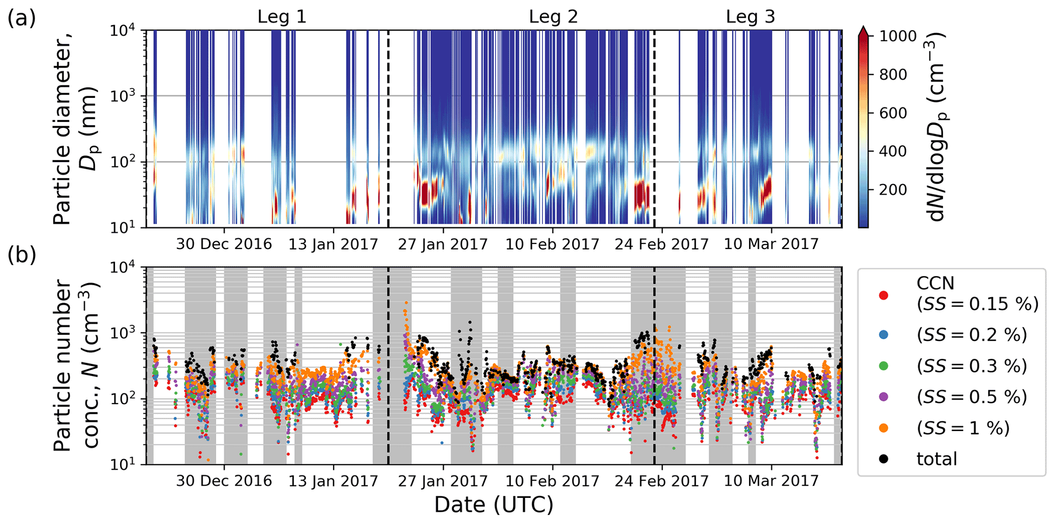
Figure 2 Time series of (a) hourly smoothed PNSD and (b) total aerosol particle (black) and CCN number concentration (colour-coded by supersaturation) during Legs 1–3. Ports visited (dashed lines) and vicinity to land (grey area) are indicated in the figure. Data gaps stem from filtering for instrument availability and exclusion of stack exhaust contamination periods. In (a) the Hoppel minimum can be seen as local minimum in the Aitken mode of the PNSD (Leg 1: 48 nm, Leg 2: 74 nm, Leg 3: 68 nm on average).

Time series of N_total and N_CCN(SS) for the ACE cruise are given in Fig. 2b. Here, days for which the average distance to land is lower than 200 km are highlighted with grey shading. Additionally, the starts and ends of the different legs are given as dashed lines. Filtering by stack exhaust contamination caused concurrent data unavailability, while differences in temporal resolution and availability of the instruments create times with no overlap between N_total and N_CCN(SS). Figure 2b shows that N_CCN at a particular SS varied over 2 orders of magnitude throughout the cruise, e.g. at a SS of 0.2 % (N_CCN,0.2) from 4 to 309 cm⁻³. In the vicinity of the ports, higher N_total and N_CCN(SS) are observed compared to the open-ocean sections (stack exhaust contamination filtering being performed for both as described in Sect. 2.2). This suggests aerosol particle abundance to be influenced by terrestrial and anthropogenic sources and is in line with Schmale et al. (2019) showing pristine conditions during ACE being encountered only south of 55^∘ S.

Periodic differences between N_total and N_CCN,1.0 throughout the cruise were observed (Fig. 2b). Periods of larger differences coincide with PNSD in Fig. 2a featuring a pronounced Aitken mode (D_p=10–100 nm) with elevated numbers in the size range below 40 nm. During these periods even SS =1 % was not sufficient to activate the smaller Aitken mode particles. Consequently, quantities presented later in this article, that are derived from N_CCN,1.0, are representative for the larger Aitken mode particles (D_crit at this SS of ∼30 nm; see Table S1 in the Supplement).

In addition to the time series presented in Fig. 2b, spatial distribution of N_CCN at all measured SS are given as daily averages in Fig. S2.

Averages of N_CCN(SS) for the legs of ACE are shown in Fig. 3a. Due to the frequency distributions of N_CCN in Fig. 4a (introduced later) resembling log-normal distributions, leg-aggregated data and variability are given as geometric mean and geometric standard deviation values, respectively. N_CCN values increase with SS, e.g. for Leg 1 from 91 cm⁻³ (N_CCN,0.15) to 241 cm⁻³ (N_CCN,1.0). For all SS values, the largest geometric mean values of N_CCN(SS) are observed during Leg 2. Moreover, the average Hoppel minimum diameter was found to be the largest for Leg 2, when compared to Legs 1 and 3, indicating a pronounced Aitken mode. This, together with Schmale et al. (2019) showing less contribution (relative and absolute) of SSA to CCN during Leg 2, suggests a significant fraction of CCN originating from secondary aerosol production. However, differences in N_CCN between legs are within the ranges given by the respective geometric standard deviations. The longitudinal differences in CCN abundance are either small against the overall variability in the data, or a variety of effects cancel each other out so that no clear longitudinal trend can be observed. A similar conclusion can be drawn in terms of latitudinal trends, because the majority of the cruise track during Leg 2 was south of 60^∘ S, compared to Legs 1 and 3 being solely north of 60^∘ S. With this, the CCN number concentrations given in Table S1 in the Supplement can be considered representative for the MBL over the whole SO region during summertime.

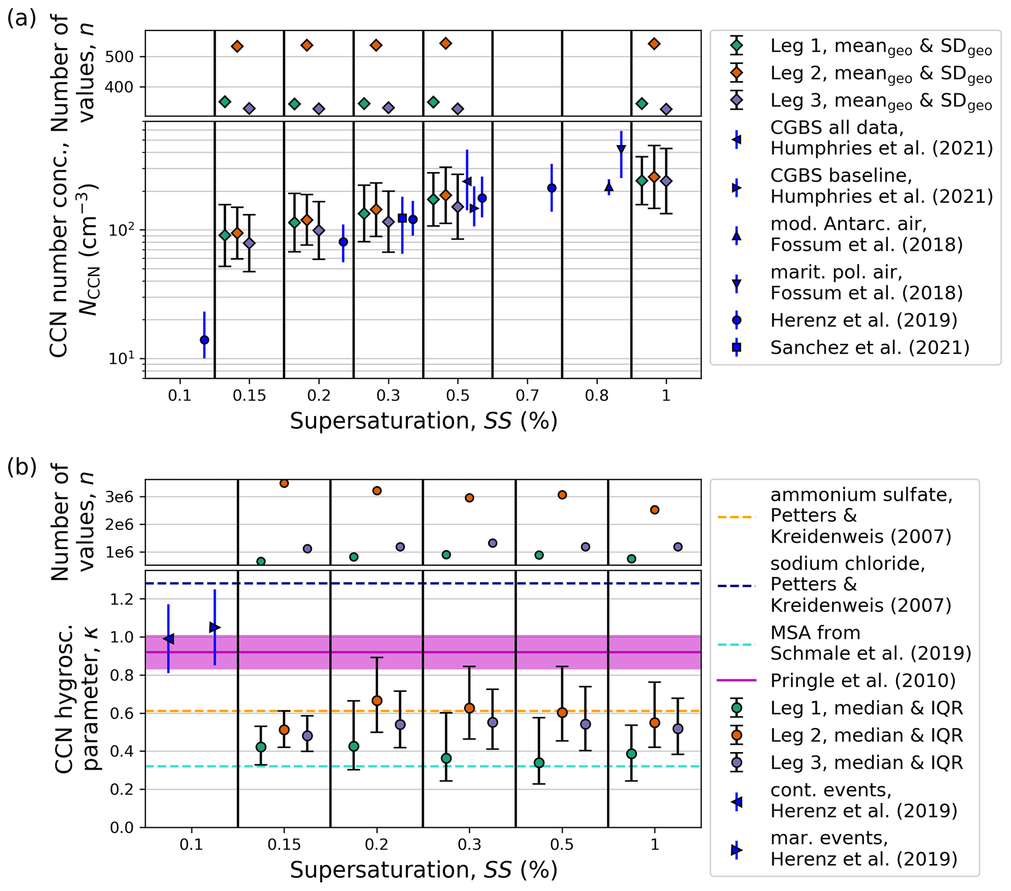
Figure 3 (a) Geometric mean values (mean_geo) and geometric standard deviation (SD_geo; whiskers) of CCN number concentration (N_CCN) and (b) median values and respective inter-quartile range (IQR) of aerosol particle hygroscopicity parameter (κ). Both N_CCN and κ are given as function of supersaturation (SS) for Leg 1 (green), Leg 2 (orange), and Leg 3 (purple), respectively. All κ values resulting from D_crit values outside of 10th to 90th percentile range for D_crit (per SS) are excluded here. Included for comparison in (a) are the averages (median and IQR) over all measurements at Cape Grim Baseline Station (CGBS) coinciding with PEGASO and CAPRICORN-II from Humphries et al. (2021) (triangle pointing left) and measurements for “baseline” conditions (triangle pointing right) during that period. Baseline conditions are defined as wind directions between 190 and 280^∘, and ambient radon concentrations below 100 mBq m⁻³. Averages for events of modified Antarctic air (upward pointing triangle) and maritime polar air (downward pointing triangle) from Fossum et al. (2018) are given. As reference, mean κ values for sodium chloride (dashed blue line) and ammonium sulfate (dashed orange line) from Petters and Kreidenweis (2007), and a hypothetical κ value for MSA from Schmale et al. (2019) (dashed teal line) is given in (b). Averages for Antarctica from Herenz et al. (2019) for cases of continental (triangle pointing left) and marine events (triangle pointing right) are given. Modelled κ values for the Southern Ocean's surface layer (magenta line and area) from Pringle et al. (2010) for reference. The number of data points (n) are indicated in the figure.

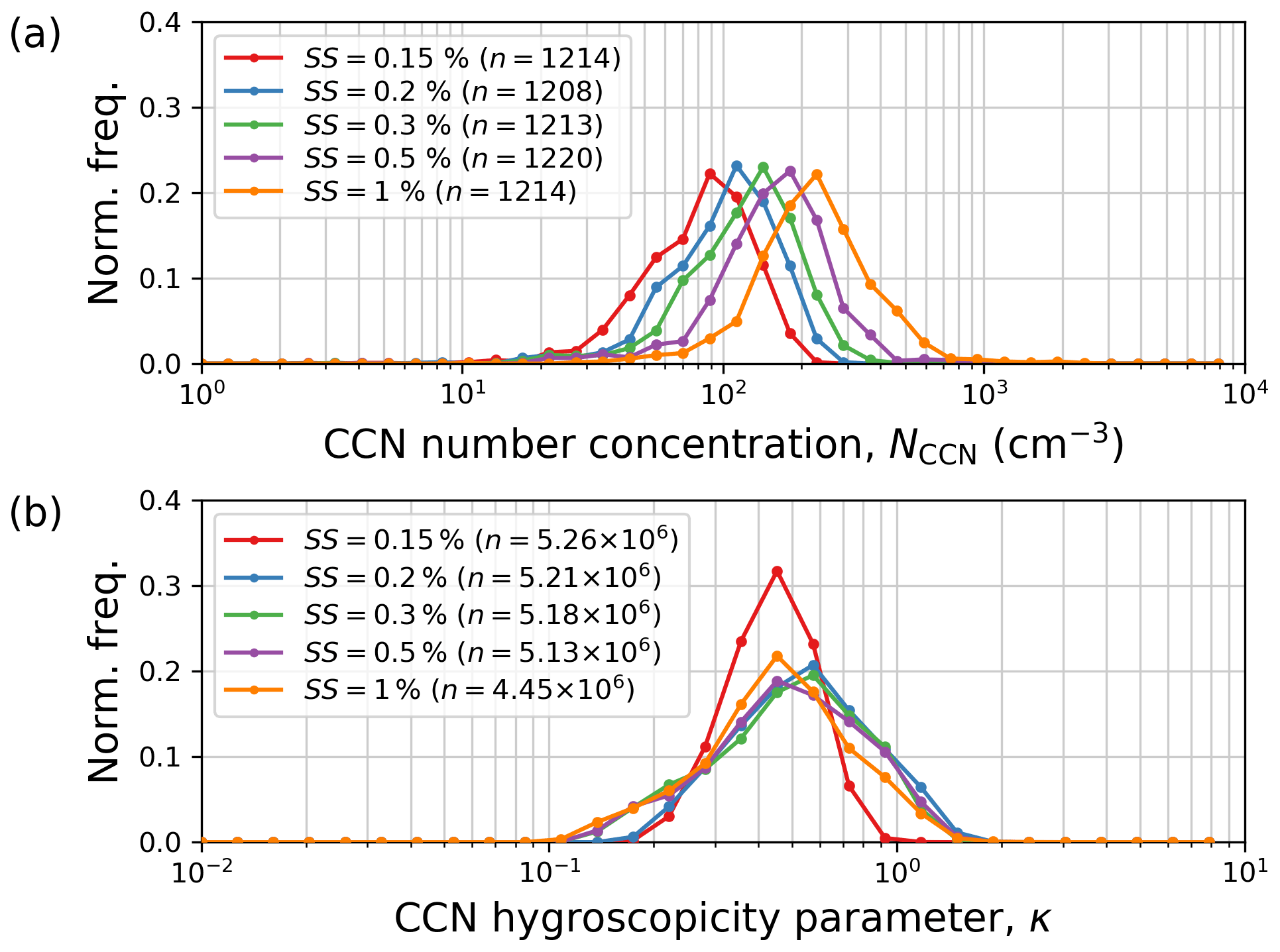
Figure 4 Normalized probability density function of (a) CCN number concentration (N_CCN) and (b) hygroscopicity parameter (κ) for levels of supersaturation 0.15 %, 0.2 %, 0.3 %, 0.5 %, and 1 % (SS, colour-coded) of all observations taken during Legs 1–3. The N_CCN result from averaging 5 min long intervals of 1 Hz measurements. Each of the six SS levels is repeated once per hour. The κ values result from Monte Carlo simulation runs (n_MCS=10⁴) of hourly smoothed particle number size distributions. All κ values that resulted from D_crit outside of 10th to 90th percentile range (per SS) are excluded. The number of data points are indicated (n) in the figure.

Herenz et al. (2019)Humphries et al. (2021)Fossum et al. (2018)Sanchez et al. (2021)Humphries et al. (2021)Sanchez et al. (2021)Humphries et al. (2021)

Table 1 Overview of a selection of studies on aerosol particles and CCN over the summertime Southern Ocean.

In addition to our data, N_CCN from a selection of other studies performed on Antarctica or over the SO are given in Fig. 3a and summarized in Table 1. For the continental Antarctic research station Princess Elisabeth (PES), located at 71.95^∘ S and 23.35^∘ E on East Antarctica's Queen Maud Land and about 200 km in-land from the Antarctic coast, Herenz et al. (2019) reported N_CCN,0.1, N_CCN,0.2, N_CCN,0.3, N_CCN,0.5, and N_CCN,0.7. Overall, we find good agreement between values for the measurement period 2013–2016 in Herenz et al. (2019) and the geometric mean values of this study covering roughly 3 months during the Austral summer. The reported values of N_CCN,0.2, N_CCN,0.3, and N_CCN,0.5 for cases of maritime air masses reaching PES show a difference of −28 %, −9 %, and +3 % to our values, respectively. A first hypothetical reason for the differences at SS =0.2 % is that PES is not located directly at the Antarctic coast. A second hypothetical reason is that activation at this low SS is associated with large particles, which might be removed due to atmospheric processes during transport to PES. At the Australian Cape Grim Baseline Station (CGBS; 40.68^∘ S, 144.68^∘ E), N_CCN,0.5 has been measured continuously since the mid-1970s (Gras and Keywood, 2017). In Humphries et al. (2021), average N_CCN,0.5 values over ACE's time frame (November 2017 to March 2018) at CGBS are given. For this period, a N_CCN,0.5 median of ∼230 cm⁻³ is reported (triangle pointing left in Fig. 3a). This is above our median value for Leg 1 of 181 cm⁻³ and at the upper end of our results (inter-quartile range (IQR): 138–225 cm⁻³). Differences could be due to continental air masses reaching CGBS. Conditions at CGBS are only representative for the SO when the wind direction is between 190 and 280^∘, the so-called “baseline” conditions (Gras and Keywood, 2017). At CGBS, the ambient radon concentration is used as a proxy for terrestrial influence (e.g. McCluskey et al., 2018a) and a threshold of 100 mBq m⁻³ is used in Humphries et al. (2021). The averaging of the CGBS measurements which feature only baseline conditions gives a median of ∼130 cm⁻³ (triangle pointing right in Fig. 3a). This is at the lower end of our results for Leg 1, and we conclude that the terrestrial influence on our N_CCN,0.5 average values is small. The terrestrial influence during Leg 1 being small is underlined later in the text by the backward trajectory analysis (see Sect. 3.2). As for ship-based CCN measurements, comparison between our findings and the PEGASO cruise in the SO's Atlantic sector during January–February 2015 (Fossum et al., 2018) can only be done semi-quantitatively, since SS are not identical. Further, a comparison is only reasonable for Leg 3, the part of ACE on the Atlantic sector of the SO. The result of visual interpolation between our N_CCN,0.5 and N_CCN,1.0 for Leg 3 lies in the ranges of 217±31 cm⁻³ reported for modified Antarctic air encountered during PEGASO (Fig. 3a). For the British Southern Ocean (BSO) cruise, only CCN number concentrations inferred from nss sulfate are available in O'Dowd et al. (1997), not comparable with any of our N_CCN. As for aircraft-based CCN measurements, N_CCN,0.3 between 17 and 264 cm⁻³, with an average of 123±58 cm⁻³ (mean±SD), are reported in Sanchez et al. (2021) for flights through the MBL between 42.5–62.1^∘ S and 133.8–163.1^∘ E during the Southern Ocean Clouds, Radiation, Aerosol Transport Experimental Study (SOCRATES). The reported concentrations are slightly lower than what was measured in that area during ACE, with values between 48 and 452 cm⁻³ and an average of 178±99 cm⁻³ (mean±SD). Besides the difference in measurement height (SOCRATES: 50 m a.s.l. until height of inversion; ACE: ∼15 m a.s.l.; see Sect. 2), another factor is that measurements are from successive years, with the ACE cruise being in that area during 16 January to 26 January 2017 and the 15 flights during SOCRATES in the period of 15 January to 25 February 2018.

An overview on the aerosol particle hygroscopicity parameter, κ, observed during Legs 1–3 is given in Fig. 3b. Leg-wise averages of the hourly available κ values per SS are given as median values and respective IQRs because the frequency distributions of κ(SS) in Fig. 4b (introduced later) do not resemble log-normal distributions. Error bars include both natural variability and the measurement uncertainty in κ, as described in Sect. 2.2. Median κ values for all legs and SS are spread between 0.3 and 0.7, with a combined variability–uncertainty range (indicated by IQR as error bars) ranging from 0.2 to 0.9. Differences between legs can be seen, with the highest median values at each SS found for Leg 2. Reference values for pure compounds or compound classes are given in Petters and Kreidenweis (2007); a mean κ between 0.1 and 0.2 for organic material, κ_mean=0.6 for ammonium sulfate, κ_mean=0.9 for sulfuric acid, and κ_mean=1.3 for sodium chloride is reported. A typical κ value for ammonium nitrate is omitted in Fig. 3b, as nitrate-containing compounds were found to not play an important role for the CCN population. Additionally, in Schmale et al. (2019) a κ∼0.3 for MSA is hypothesized. The majority of our κ values are above what is given for organic material and below the value given for sulfuric acid, which indicates that the sampled CCN population consists of a variable mixture of organic and inorganic materials. Median κ values for Leg 1 are closest to what is assumed for MSA, while median values for Legs 2 and 3 are closer to the value for pure ammonium sulfate. Looking at size dependency, no clear trend in κ values between different SS is apparent when considering error bars. For the size range between roughly 30 and 110 nm probed by the range of SS (Table S1 in the Supplement), the chemical composition appears to be independent of particle size, which further suggests a well-mixed aerosol (or CCN) population. However, when considering median values alone, for SS >0.15 % a slight decrease in κ values with increasing SS can be seen for Leg 2. Lower κ values at higher SS are in line with condensable organic vapours contributing to the aerosol chemical composition, while larger, aged particles activating at lower SS are associated with higher κ values (McFiggans et al., 2006). Legs 1 and 3 do not feature increasing κ values with decreasing SS, which suggests an internally mixed CCN population.

Comparison to Herenz et al. (2019) shows that our κ values observed over the SO are much lower than the ones reported for the austral summer on continental Antarctica, where κ values at SS =0.1 % were found to be in the range between 0.8 and 1.3. This suggests significantly different particle composition at PES compared to the SO. Herenz et al. (2019) interpreted their sampled particles to be of mostly inorganic nature (i.e. sea salt) and therefore assumed a primary, marine origin. Our values, because of the overall small κ values, hint towards a composition dominated by organics. Note that particle sizes between 30 and 110 nm were probed with the SS range of our instrument, hinting at the encountered aerosol population being mainly comprised of smaller particles. For SOCRATES, Saliba et al. (2020) report κ values between 0.2 and 0.5 for particles with D_p<100 nm. Our κ values in this size range (corresponding to SS >0.2 %) lie partially in a similar range (Leg 1) and partially on the upper end (Legs 2 and 3) of the range found during SOCRATES, respectively.

Using a global numerical weather model, simulations of κ values at SS =0.1 % for the SO region were presented in Pringle et al. (2010). Model results give values of 0.9±0.1 for the surface layer. Comparison to our results suggests an overestimation of sea salt contribution and/or an underestimation of the presence of organic material in the model. A similar effect is noted in Schmale et al. (2019), when the N_CCN,0.2 values measured during ACE are compared to the output of the Global Model of Aerosol Processes (GLOMAP). The largest differences between measurements and model output coincided with the highest gaseous MSA concentrations, suggesting an underestimation of CCN from secondary origin. A global model producing κ values for the SO region twice as high compared to what we measured in situ reveals a strong discrepancy in CCN properties and suggests possible model deficiencies in the representation of CCN sources and modelled aerosol–cloud interactions.

Geometric mean values (and respective geometric standard deviation) of N_CCN and D_crit and median values (and respective IQR) of κ for the entire cruise and its legs are summarized in Table S1 in the Supplement.

Probability density functions (PDFs) of normalized frequencies for N_CCN(SS) and κ(SS) during Legs 1–3 are given in Fig. 4. PDFs of N_CCN (Fig. 4a) show mono-modal distributions for all SS, with the PDF maxima shifting towards higher N_CCN with increasing SS, e.g. ∼90 cm⁻³ at 0.15 % to ∼210 cm⁻³ at 1 %. Comparing the distribution for N_CCN,0.2 (blue line in Fig. 4a) with yearly-averaged PDFs from measurement sites around the globe in Schmale et al. (2018), our values show lower number concentrations with a PDF maximum at ∼100 cm⁻³ and share resemblance in terms of number of modes and maximum location with the distribution reported for clean marine conditions (mono-modal, maximum at ∼200 cm⁻³). For the MBL legs of SOCRATES, the PDF for N_CCN,0.3 is bi-modal, with peaks at 100 and 150 cm⁻³ (Sanchez et al., 2021). In their study, the low concentration mode was associated with precipitation events, effectively removing larger particles. The high concentration mode was associated with atmospheric processes causing particle growth, e.g. (1) oxidation of volatile organic compounds and subsequent condensation or (2) cloud processing.

A change in distribution shape with increasing SS can be seen for PDFs of κ(SS) in Fig. 4b. All five distributions are mono-modal, with maxima between 0.4 and 0.6. PDFs for SS of 0.3 %, 0.5 %, and 1 % (green, purple, and orange line, respectively) feature a tail towards smaller values of κ. This occurrence of small particles (activated at high SS) consisting of mainly organic material forms a strong case for the sampled Aitken mode CCN originating from secondary organic aerosol formation and growth processes. The accumulation mode, probed with the measurement at SS =0.15 %, shows similar κ values to the Aitken mode (Fig. 4b).

PDFs for all SS other than 0.15 % feature a tail towards higher κ values. Such high κ values at high SS seem counter-intuitive and are indicative of highly hygroscopic Aitken mode particles being sampled. A sensitivity study of our methodology with respect to (1) modelling the measurement uncertainty via Monte Carlo simulations (Fig. S3a), (2) consideration of error propagation, and (3) quality of the fitted modes to the PNSD was performed. As κ values were robust against these variations, we conclude that this tail (while counter-intuitive) is not an artefact of our methodology. However, to avoid speculation on the reason, we take a conservative approach in keeping the focus of the interpretation on the median values presented in Fig. 3b.

3.2 Ice-nucleating particles

Time series of N_INP(T) for $T=-\mathrm{24}$ ^∘C ($N_{\mathrm{INP},-\mathrm{24}}$; orange), $N_{\mathrm{INP},-\mathrm{20}}$ (purple), $N_{\mathrm{INP},-\mathrm{16}}$ (blue), $N_{\mathrm{INP},-\mathrm{12}}$ (green), and $N_{\mathrm{INP},-\mathrm{8}}$ (magenta) are given in Fig. 5a–e, respectively. INP number concentrations outside the detectable range (indicated by triangles and estimated as described in Sect. 2.3) are represented in the figure by each filter's lowest (lower detection limit) and highest resolvable concentration value (upper detection limit). For $T\le -\mathrm{12}$ ^∘C (Fig. 5a–d), the respective measurement background INP number concentrations are represented via the averaged FBF spectra (dashed–dotted lines), as described in Sect. 2.3. Measurement uncertainties (indicated by error bars) become smaller with decreasing temperature. This is due to (1) increased freezing probability with decreasing temperature and (2) the measurement uncertainty being described by binomial sampling confidence intervals (following Agresti and Coull, 1998). The combination of both effects results in smaller error bars at lower temperatures. At −12 and −16 ^∘C, N_INP values show the highest variability of around 3 orders of magnitude. At −8 and −20 ^∘C the variability decreases to about 2 orders of magnitude, while $N_{\mathrm{INP},-\mathrm{24}}$ only varies within 1 order of magnitude. This decrease in the range of values is considered a bias due to N_INP being close to or above the upper detection limit. Each of the shown time series of N_INP in Fig. 5 contains episodes of elevated INP number concentrations, coinciding with the RV being close to land (grey area; within 200 km) and ports (dashed line). During the open-ocean sections of the cruise the majority of data points show concentrations up to 2 orders of magnitude lower (e.g. $N_{\mathrm{INP},-\mathrm{16}}=\mathrm{0.1}$–10 m⁻³). This suggests that elevated atmospheric INP concentrations are connected to terrestrial (including coastal) INP sources. This assumption is supported by the results of the air-mass origin analysis (Sect. 2.4) using the LAGRANTO backward trajectories for ACE provided in Thurnherr et al. (2020). An overview of the results is given in Fig. S6 showing time series of surface contributions to each LV filter. The time series for the surface type contributions to the PBL signal (Fig. S6c) and the contribution of geographical regions (Fig. S6d) show that periods of elevated INP number concentration (Fig. 5) coincide with periods when air masses that passed over African, Australian, and South American land masses or coastal regions were sampled. Contrary to these regions, air masses passing over Antarctica did not show higher N_INP than oceanic air masses (Fig. S7).

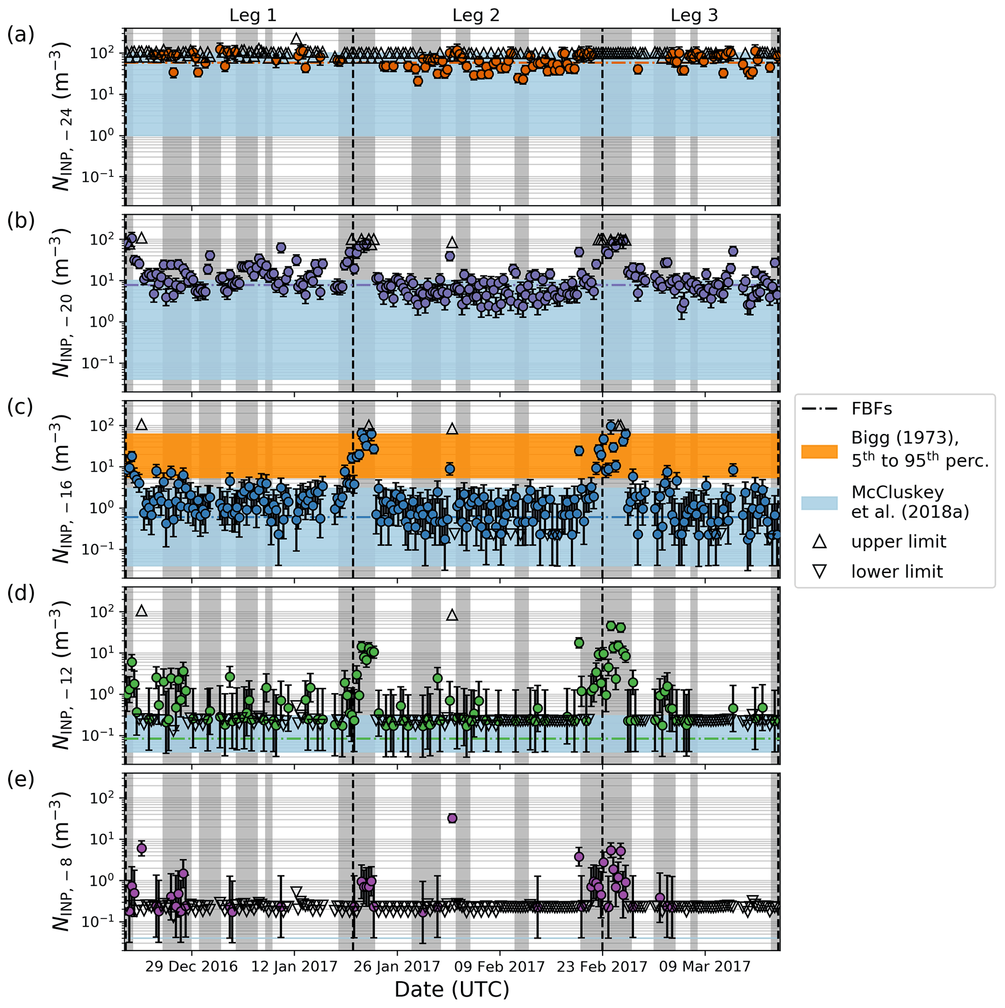
Figure 5 Time series of INP number concentration (N_INP) at (a) −24, (b) −20, (c) −16, (d) −12, and (e) −8 ^∘C from the LV filters sampled during ACE. N_INP values outside the detectable range are indicated by downward (upward) pointing triangles if they are below (above) the lower (upper) edge of the detectable range. The legs of ACE (dashed lines) and periods when the RV was close to land (grey area) are indicated. In (a)–(d) the measurement background from averaged spectra of field blank filters (FBFs) is indicated (dashed–dotted lines). N_INP values from McCluskey et al. (2018a) are included for reference (blue area). In addition, $N_{\mathrm{INP},-\mathrm{15}}$ values from Bigg (1973) are included in (c) as the range between their 5th and 95th percentile (orange area). A correction of the $N_{\mathrm{INP},-\mathrm{15}}$ values from Bigg (1973) was applied, following the supporting information to McCluskey et al. (2018a).

For comparison, Fig. 5c contains the range between the 5th and 95th percentile of $N_{\mathrm{INP},-\mathrm{15}}$ from Bigg (1973) (orange area). They sampled filters over the SO around Australia, collecting 0.3 and 3 m³ of ambient air through a pair of membrane filters. In terms of sampling strategy, our LV sampling of 12 m³ through a porous filter over 8 h compares well with the sampling of Bigg (1973). The techniques to measure N_INP were, however, different. Filters sampled during ACE were analysed with a freezing array method (Sect. 2.3), while INP contents in Bigg (1973) were analysed by means of a thermal diffusion chamber. In the Supplement of McCluskey et al. (2018a), the effect of background INP concentrations during the study of Bigg (1973) is assessed and a correction proposed (22 % lower values). This correction was applied to the values shown in Fig. 5c. The majority of our $N_{\mathrm{INP},-\mathrm{16}}$ measurements are in the open-ocean sectors and clearly below the range of $N_{\mathrm{INP},-\mathrm{15}}$ observed by Bigg (1973). However, the $N_{\mathrm{INP},-\mathrm{16}}$ values larger than 10 m⁻³ at the end of Leg 1, when the RV was in the vicinity of Australia, lie within the range of values given in Bigg (1973).

In McCluskey et al. (2018a) INP measurements from CAPRICORN-I are presented. The range of observed INP concentrations is included in Fig. 5 for comparison. At each temperature, N_INP values observed during ACE are at the upper end or higher than concentrations observed during CAPRICORN-I, except at −16 ^∘C when low concentrations were measured on the open ocean in air masses without terrestrial influence. Differences in sampled geographical area (CAPRICORN-I: 43–53^∘ S and 141–151^∘ E; this study: 34–78^∘ S, circum-Antarctic) and season (CAPRICORN-I: March–April; this study: December–March) could be reasons for the differences in observed INP abundance. Our results are consistent with preliminary results from MARCUS, CAPRICORN-I & II in McFarquhar et al. (2021), where N_INP values in the MBL over the SO are shown to exhibit a large variability, very low overall values, and a weak overall latitudinal dependence. Further, the highest concentrations were found near land, and values differed largely from historical measurements (e.g. Bigg, 1973). Feedback of the Earth's changing climate on INPs in the SO region as a contributor to the observed difference between current and historical observations cannot be ruled out (e.g. Bigg, 1990). However, potential mechanisms behind such hypothetical feedback have not been identified so far. For completeness, spatial distributions of $N_{\mathrm{INP},-\mathrm{16}}$ from our study and $N_{\mathrm{INP},-\mathrm{15}}$ from Bigg (1973) are shown in Fig. S4c.

Averaging of the N_INP at selected temperatures has been performed, in order to showcase typical values for the SO region. A summary of average INP concentrations for Legs 1–3 at selected temperatures is given in Table S2. Two different approaches were used for averaging the INP concentrations of the LV samples. In the first approach only values which are inside the detectable range are considered, and the averages are given as N_INP,LV in Table S2. For the second approach, values outside the detectable range $\left(N_{\mathrm{INP},\mathrm{LV}}^{\ast }\right)$ were included by using a value on the edge of the detectable range instead (see Sect. 2.3). Results of the two approaches differ in mean, median, and geometric mean concentration values by up to ±50 %. The largest differences were found at a T of −8 and −24 ^∘C, where the number of data points outside the detectable range is largest. We report all averaged values with explicit reference to their potential biases.

Average values of $N_{\mathrm{INP},-\mathrm{24}}$, $N_{\mathrm{INP},-\mathrm{20}}$, $N_{\mathrm{INP},-\mathrm{16}}$, $N_{\mathrm{INP},-\mathrm{12}}$, and $N_{\mathrm{INP},-\mathrm{8}}$, sorted by legs of ACE, are given in Fig. 6. Values were determined including the estimates for INP concentrations outside the detectable range (triangles in Fig. 5). As a point of reference for the measurement background, concentrations of the averaged FBF are included (dashed–dotted lines). Differences in median values between different legs are largest at −20 ^∘C, though still within the respective IQR. Mean values (crosses in Fig. 6) are higher than the median, and outside of the IQR for all temperatures other than −24 ^∘C.

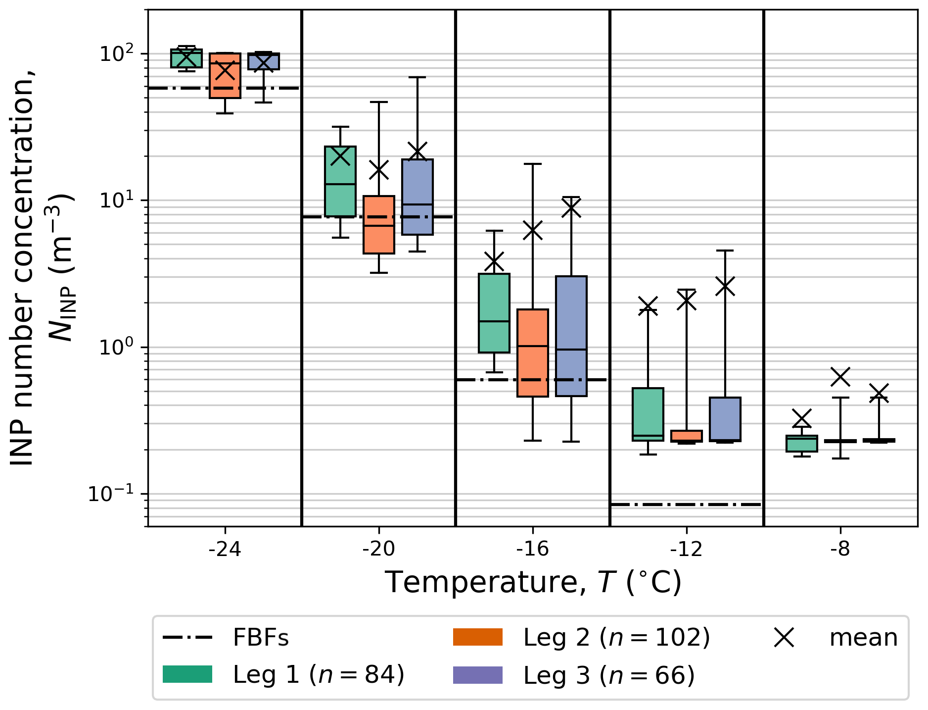
Figure 6 Mean values (crosses) and box-and-whiskers plots indicating the median (horizontal lines), inter-quartile range (boxes), and 10th to 90th percentiles (whiskers) of INP number concentration (N_INP) from the LV filters sampled during Leg 1 (green), Leg 2 (orange), and Leg 3 (purple). Averaging was performed by treating zero (infinite) values of N_INP at given temperature as values of the lower (upper) limit of the detectable range. In the figure, the measurement background is represented by the averaged spectra of the field blank filters (FBFs; dashed–dotted lines), and the number of data points (n) are indicated.

The air-mass origin for the whole cruise and individual legs are presented in Fig. 7. The average contributions for the whole cruise are dominated by air masses from the open ocean, with contributions of at least 80 % and up to 97 % (Leg 1). The terrestrial air masses (land and coast; excluding Antarctica) contribute only between 2 % (Leg 1) and 12 % (Leg 3). Similar leg-wise average contributions could, hypothetically, be a result of the dominant contribution of “open-ocean” conditions during all legs combined with limited INP variability over the entire SO for “open-ocean” conditions.

Figure 7 Percents of surface type over-passed by 10 d backward trajectories (see Sect. 2.4 and Text S1 in the Supplement for details). Colour codes for surface types are non-Antarctic land masses (red), non-Antarctic coastal regions or islands (orange), Antarctic continent or coastal regions (ANT; yellow), ice-covered regions (light blue), and open ocean (dark blue). From left to right, the different surface contributions to the air masses are shown for the entire circumnavigation (Legs 1–3), separated by leg (see Fig. 1), and cases of $N_{\mathrm{INP},-\mathrm{20}}$ below (“low”) or above 40 m⁻³ (“high”), $N_{\mathrm{INP},-\mathrm{16}}$ below/above 10 m⁻³, and $N_{\mathrm{INP},-\mathrm{12}}$ below/above 4 m⁻³ are analogous to ranges indicated in the respective PDF (see Fig. 8b–d). The number of trajectory clusters (n) are indicated in the figure. Trajectory maps for ACE are available at an hourly resolution from Thurnherr et al. (2020).

PDFs of N_INP at selected temperatures are shown in Fig. 8. N_INP(T) values outside of the detectable range are not considered for the PDF. As an indication for the detectable range, averages for the upper and lower concentration limit are indicated in Fig. 8c–e (dashed line). Interpretation of the PDFs for $N_{\mathrm{INP},-\mathrm{8}}$ and $N_{\mathrm{INP},-\mathrm{24}}$ is omitted due to the low number of samples compared to other temperatures and concentrations being close to the FBFs, respectively. Also, for the other temperatures, the overall number of samples considered in the PDF is small. Hence, the following discussion has to be considered semi-quantitative in consequence. The $N_{\mathrm{INP},-\mathrm{12}}$ and $N_{\mathrm{INP},-\mathrm{16}}$ PDFs (Fig. 8c and d) are tri-modal, and the $N_{\mathrm{INP},-\mathrm{20}}$ PDF (Fig. 8b) is bi-modal. The lowest concentration mode for $N_{\mathrm{INP},-\mathrm{12}}$ and $N_{\mathrm{INP},-\mathrm{16}}$ contains concentrations below 0.2 m⁻³, which are on the lower boundary of the detectable range. Attributing these concentrations to a source or geographical origin is ambiguous when considering the FBF as a point of reference for the background freezing signal. FBF concentrations are 0.08 and 0.59 m⁻³ for −12 and −16 ^∘C, respectively (Table S3). We therefore only discuss the two highest concentration modes in the following. The second (first) mode of $N_{\mathrm{INP},-\mathrm{12}}$ and $N_{\mathrm{INP},-\mathrm{16}}$ ($N_{\mathrm{INP},-\mathrm{20}}$), referred to as “low concentration mode” in the following, covers a range of concentration values (e.g. $N_{\mathrm{INP},-\mathrm{16}}=\mathrm{0.3}$–10 m⁻³) encountered mainly during the open-ocean sections of the cruise (Fig. 5b–d). The analysis of the air-mass origin in Fig. 7 shows that air masses reaching the RV during the sampling of this mode contained mainly open-ocean signal (∼90 %) and only small contributions from either Antarctic (6 %), marine ice-covered regions (MIZ/sea ice; 2 %), or coastal regions (1 %). In consequence, we interpret this mode to be dominated by INPs of marine origin potentially including some long-range-transported terrestrial or coastal INPs. This mode is therefore labelled as “open ocean” (light blue area) in Fig. 8b–d. Moallemi et al. (2021) show that fluorescent primary biological aerosol particles (PBAPs) measured during the open-ocean sections of ACE originate mainly from SSA. PBAPs were found to act as INPs in several studies in marine regions of the Northern Hemisphere (e.g. McCluskey et al., 2018b; Hartmann et al., 2021), and we assume the same to be the case for the Southern Hemisphere. Therefore, we conclude PBAP from SSA to be a potential source for the INPs measured on the open-ocean sections of the cruise.

Figure 8 Normalized probability density functions (solid black line) and geometric mean values (dotted black line) for INP number concentrations (N_INP) at (a) −24, (b) −20, (c) −16, (d) −12, and (e) −8 ^∘C from the LV filters sampled during ACE. For reference, $N_{\mathrm{INP},-\mathrm{16}}$, $N_{\mathrm{INP},-\mathrm{12}}$, and $N_{\mathrm{INP},-\mathrm{8}}$ for Cabo Verde (North Atlantic; Welti et al., 2018) are given in (c)–(e), respectively (blue). Additionally, $N_{\mathrm{INP},-\mathrm{15}}$ from Bigg (1973) for data points south of 43^∘ S (orange) is given for comparison. A classification of modes based on sampling location and air-mass origin is given (yellow area: terrestrial/coastal; light blue area: open ocean). Averages of the upper (dark red) and lower concentration limit (dark blue) are indicated by dashed lines. The number of data points (n) are indicated in the figure.

The high concentration mode in the PDF of $N_{\mathrm{INP},-\mathrm{12}}$, $N_{\mathrm{INP},-\mathrm{16}}$, and $N_{\mathrm{INP},-\mathrm{20}}$ consists of values (e.g. $N_{\mathrm{INP},-\mathrm{16}}=\mathrm{10}$–100 m⁻³) measured close to land (Fig. 5b–d). This mode has a greater terrestrial and coastal influence (combined ∼35 %) than the low concentration mode, based on the air-mass origin analysis (Fig. 7). In consequence, the high concentration mode is labelled “terrestrial/coastal” in Fig. 8b–d (yellow area).

In Fig. 8c, a PDF of $N_{\mathrm{INP},-\mathrm{15}}$ from Bigg (1973) is included (orange line). Here, only a subset of the total of 126 data points from Bigg (1973) is shown, containing the 58 data points south of 43^∘ S, mimicking the latitudinal range of the ACE cruise for a better comparison (Fig. S4). Differences between $N_{\mathrm{INP},-\mathrm{16}}$ from this study and $N_{\mathrm{INP},-\mathrm{15}}$ from Bigg (1973) are clearly visible, with over 1 order of magnitude lower maximum N_INP observed in our study. Agreement of their values is highest with the subset of our observations in the proximity to land. In a recent study, Cornwell et al. (2020) have shown that re-emission of dust particles from sea water into the atmosphere is possible and that the re-emitted particles retained their ability to act as INPs. However, quantifying the contribution of this potential source is not possible with our data set.

Welti et al. (2018) presented PDFs of N_INP(T) based on filters sampled at a fixed location on the Cabo Verde island of Sao Vicente, over a 4-year period (2009–2013). The PDFs comprise changes in season, air-mass origin, and bulk aerosol composition. The respective PDFs of $N_{\mathrm{INP},-\mathrm{16}}$, $N_{\mathrm{INP},-\mathrm{12}}$, and $N_{\mathrm{INP},-\mathrm{8}}$ are included for comparison in Fig. 8c–e. Welti et al. (2018) found log-normal distributions for all temperatures, and attributed them to random dilution during transport, indicating a lack of strong local sources. In other words, the PDFs are thought to represent background INP concentrations at the Cabo Verde islands. Comparing PDFs, it can be seen that for $N_{\mathrm{INP},-\mathrm{16}}$ the bulk of our values is below what is reported in Welti et al. (2018), shifted by roughly 1 order of magnitude towards lower concentrations. For $N_{\mathrm{INP},-\mathrm{12}}$ a respective shift is not as clearly seen; however, a tendency towards more frequent occurrence of higher concentrations compared to our study is obvious. For $N_{\mathrm{INP},-\mathrm{8}}$ this tendency is not visible anymore. The difference between the PDFs given in Welti et al. (2018) and our study for $N_{\mathrm{INP},-\mathrm{12}}$ and $N_{\mathrm{INP},-\mathrm{16}}$ illustrates the latitudinal difference in marine N_INP with lower concentrations in the SO compared to the Atlantic.

The temperature spectra of N_INP for all LV filters sampled during ACE are given in Fig. S8a. The highest freezing onset was found at −4 ^∘C. Between filters, N_INP is spread over up to 3 orders of magnitude at individual temperatures. This mirrors what can be seen in the PDF in Fig. 8. A typical, steady increase in N_INP with decreasing temperature (1 order of magnitude per 5 K) can be observed for the majority of filters and the averaged FBF's curve (pink line). At higher temperatures ($>-\mathrm{20}$ ^∘C) a shoulder in the INP spectra of a number of filters is apparent. This feature is unlike those previously mentioned, steady increase in N_INP. A high concentration of INPs above −15 ^∘C is typically associated with a signal of a biological INP source mixed with a mineral or less efficient INP source (e.g. Creamean et al., 2019). In the range of −12.5 to −22.5 ^∘C, only the lowest curves of our spectra lie within the range observed by McCluskey et al. (2018a), who observed even lower N_INP over the SO.

In order to test the hypothesis that typical marine INPs (e.g. SSA) were encountered for the majority of the cruise, concentration values were normalized. This was achieved by dividing N_INP by the particle surface area concentration or the particle volume concentration derived from the total aerosol particle number size distributions under the assumption of spherical particles (see Sect. 2.3). Normalization enables comparison of INP properties across different studies, which can include different N_INP derivation approaches or sampled particle size ranges, independent of N_INP. The resulting spectra of ice-active number site density, n_s, and volume site density, n_v, are given in Fig. S8b and c. Values of n_s spread over 4 orders of magnitude (0.1–1000 cm⁻²) in the observed temperature range. For comparison, values from two laboratory experiments are included in Fig. S8b, which focused on sampling of artificially generated SSA and assessing its ice activity (DeMott et al., 2016; Mitts et al., 2021). The results from DeMott et al. (2016) span a wider range of n_s and T than the ACE data, while values from Mitts et al. (2021) overlap with the open-ocean-sampled filters from ACE. Field measurements from CAPRICORN-I (McCluskey et al., 2018a) showing a large variability in n_s are included for comparison. Contrary to N_INP (Fig. S8a), n_s values from ACE lie within the lower end of what is reported from CAPRICORN-I. This indicates observation of a similar or more ice-active particle population during CAPRICORN-I compared to ACE. The ranges of n_v reported in Mitts et al. (2021) are included in Fig. S8c for comparison. The range overlaps with the lower range of the values from ACE. In conclusion, the strong overlap between ice-active site density profiles from ACE (derived from N_INP) and studies of artificial SSA (e.g. DeMott et al., 2016; Mitts et al., 2021) supports the idea that low N_INP measured on the open ocean might be driven by SSA.

As mentioned in Sect. 2.3, HV filters were also analysed for INPs, but due to better higher data coverage (LV: n_filter=253; HV: n_filter=79) we focused on the LV samples. For the sake of completeness we give in Fig. S5 the additional INP spectra determined from HV samples (DHA-80 sampler). Compared to the LV results in Fig. S8a, the determined N_INP(T) are higher and in a narrower range. LV and HV samples differ in sample collection interval and filter material (LV: poly-carbonate pore filter, 200 nm pore size; HV: quartz fibre filter). Concerning collection intervals, continuous sampling over 8 h intervals were chosen for the LV filters to resolve diurnal N_INP variations (non-detected). HV filters were collected during intervals of 24 h, interrupted by breaks due to the automatic shutdown to avoid contamination from ship exhaust. Possible low biases of N_INP for higher sampled volumes have been discussed in Bigg et al. (1963) and Mossop and Thorndike (1966) but do not reflect the trend found for our two sampling techniques. There could be an averaging effect from the longer sampling interval for the HV filters, when sampling from an unevenly distributed INP population. However, such effects require further investigation. The differences in filter material could be another factor but are in contrast to Wex et al. (2020) finding good agreement between quartz fibre and poly-carbonate filters for identical sampling intervals. The higher background INP levels for the HV filters, indicated by higher N_INP,FBF compared to the LV sampling (Table S3), hints towards a limited ability of the HV sampling to measure lower INP number concentrations and in consequence overall higher measured INP number concentrations. Contamination from ship exhaust should not effect INP analysis results (see Appendix C in Welti et al., 2020) as exhaust particles are not ice-active in the investigated temperature range. However, deactivation of some INPs due to exhaust contamination cannot be ruled out.

3.3 Analysis of sodium and MSA

Information on the aerosol chemical composition is widely used to infer the origin of the sampled aerosol particles. To aid the characterization of CCN and INP sources over the SO, sampled HV filters were analysed regarding the aerosol load and the atmospheric particle mass concentrations of sodium and MSA, two compounds known to be unaffected by stack exhaust.

On average, 32.4 µg m⁻³ (median; IQR: 26.1–49.6 µg m⁻³) of PM₁₀ was observed during ACE (Table S5). Leg 1 exhibits a higher median value (42.4 µg m⁻³) compared to Legs 2 and 3 (31.1 and 33.3 µg m⁻³). Note that contrary to sodium and MSA (see Sect. 2.3), an influence of the RV's ship exhaust on PM₁₀ mass cannot be ruled out. However, the quantification of this potential influence is beyond the scope of this study.

Averaging sodium mass concentrations for the whole cruise gives a median value of 2.8 µg m⁻³, with an IQR from 1.8 to 3.9 µg m⁻³ (Table S5). Higher median values for Legs 1 and 3 compared to Leg 2 are found, similar to what is observed for PM₁₀. This is consistent with Blanchard and Woodcock (1957) showing SSA production to be driven by wave breaking and Schmale et al. (2019) showing on average higher wind speeds and significant wave heights for the legs with extended open-ocean sections (Legs 1 and 3). For the 34th Chinese National Antarctic and Arctic Research Expeditions (CHINARE) cruise over the SO (40–76^∘ S, 170^∘ E–110^∘ W) in February–March 2018, Yan et al. (2020c) report an average sodium mass concentration of 0.8±0.8 µg m⁻³ (mean±SD). During Leg 2 of ACE, the part of the cruise that has the largest geographical overlap with the region covered during CHINARE, the median sodium mass concentration was 1.8 µg m⁻³, i.e. more than 2 times higher than that observed during CHINARE.

MSA mass concentrations were generally 2 orders and 1 order of magnitude lower than the ones for PM₁₀ and sodium, respectively. Consequently, values are reported in ng m⁻³ in the following. A median mass concentration of 102 ng m⁻³ for the entire ACE cruise was found (Table S5), with highly variable values ranging from 1 to 455 ng m⁻³. Differences in median values between legs are very small. The highest mass concentration of 455 ng m⁻³ was observed on the Ross Sea close to the Antarctic coast (Leg 2). Davison et al. (1996) report for south of the Falkland islands in November 1992 a mean MSA mass concentration of 27 ng m⁻³, with values ranging up to 99 ng m⁻³. During ACE in late February of 2017, values around 120 ng m⁻³ were found in this part of the SO between 70–36^∘ W. Besides long-term trends over the last two decades, the difference of up to 1 order of magnitude might be due to the difference in season, with higher mass concentrations for ACE due to increased marine biological activity in early fall compared to late fall for Davison et al. (1996). Another factor is the large degree of variability in MSA abundance across the SO, depending on season and location as illustrated in Castebrunet et al. (2009), with values during ACE on the higher end of the scale.

For a number of CHINARE Antarctic cruises, MSA mass concentrations are reported. Yan et al. (2020b) report for the polynya regions of the Ross Sea (50–78^∘ S, 160–185^∘ E) an average value of 44±22 ng m⁻³ (mean±SD) for December of 2017 and 39±28 ng m⁻³ for January 2018. The maximum mass concentration of 211 ng m⁻³ was reported for the Ross Sea, at around 64–67^∘ S, connected to the position of the dynamic sea ice edge at ∼64^∘ S. Here, with the start of the sea ice melting in early December, the release of iron from ice into the water can spur marine microbial activity (Turner et al., 2004), which may result in an increased DMS emission and consequently secondary MSA production. Consistently, the maximum MSA mass concentration during ACE was encountered near the sea ice edge (∼70^∘ S) of the Ross Sea in early February 2017. For the Amundsen Sea (40–76^∘ S, 170^∘ E–110^∘ W) in February–March 2018 (34th CHINARE cruise), average MSA mass concentrations of 31±17 ng m⁻³ are reported in Yan et al. (2020c). The ACE cruise went on the Amundsen Sea in early February 2017, and MSA mass concentrations in this region show a median value of 210 ng m⁻³. Overall, a difference in average MSA mass concentrations of up to 1 order of magnitude between our study and the CHINARE cruises becomes apparent. One factor might be the usage of different instrumentation and analysis techniques. Another factor causing year-to-year variability could be the presence of sea ice. Schmale et al. (2019) note a significantly lower sea ice extent on the Amundsen Sea during ACE when compared to climatological records. The lack of a sea ice cover enables marine activity and the emission of aerosol precursors into the air. Additionally, variations in atmospheric MSA sink strength are a potential contributor to variability in observed MSA mass concentrations. For example, MSA is efficiently removed from the atmosphere by precipitation. In the SO, rain events are associated with frontal zones. For South Georgia, a sub-micron (PM₁) MSA mass concentration of up to 200 ng m⁻³ was reported in Schmale et al. (2013). During ACE, the RV was on station close to this island in the beginning of March 2017, with MSA mass concentrations around 75 ng m⁻³ during these days, underlining the high variability in MSA abundance over the SO.

3.4 Correlation analysis

The results of a correlation analysis performed with a selection of variables gathered during ACE is given as a Spearman rank correlation matrix in Fig. 9.

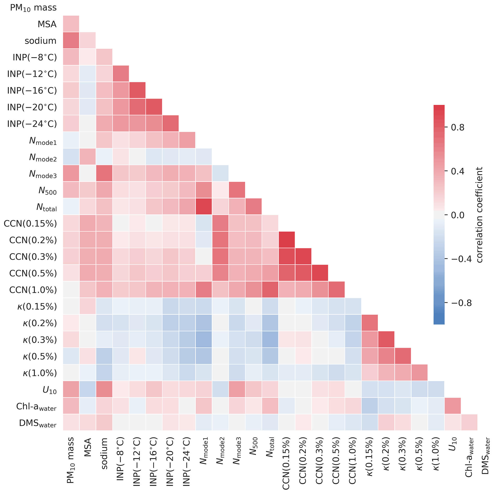
Figure 9 Spearman rank correlation matrix of quantities directly measured or derived from measurements during ACE. From the 24 h long HV sampling, PM₁₀ mass and mass concentrations of particulate sodium and MSA are included. INP number concentrations at temperatures of −8, −12, −16, −20, and −24 ^∘C (INP(T)) are included from the LV filters, sampling for 8 h. Here, the estimates for INP concentrations above and below the detection limit are included. From hourly smoothed particle number size distributions, the total particle number concentration (N_total), respective three modes (N_mode1, N_mode2, and N_mode3), and the number concentration of particles larger 500 nm in diameter (N_>500) are included. CCN number concentration at 0.15 %, 0.2 %, 0.3 %, 0.5 %, and 1 % supersaturation (CCN(SS)) and derived aerosol particle hygroscopicity parameter (κ(SS)) are included. Additionally, daily-averaged wind speed at 10 m a.s.l. (U₁₀) and in-water concentrations of chlorophyll-a (Chl-a_water) and dimethyl sulfide (DMS_water) are used. Positive correlation between two quantities indicates a similar trend over time, while an opposing behaviour is indicated by a negative correlation coefficient.

With regards to the results of our in situ aerosol particle measurement, N_total was found to be correlated with N_mode1 (correlation coefficient ρ=0.9, p<.001) and N_CCN,1.0 (ρ=0.8, p<.001). This mirrors the behaviour these quantities show in Fig. 2a and is indicative for the importance of Aitken mode particles for the total particle and CCN number concentrations at high SS.

Correlations between sodium and mode 3 (ρ=0.7, p<.001) as well as PM₁₀ (ρ=0.7, p<.001) concentrations were found. As sodium is used as a conservative tracer for primary aerosol particles of marine origin (Legrand and Pasteur, 1998), especially sea salt, the correlations suggest that SSA significantly contributes to both PM₁₀ and the coarse mode. However, we do not find a significant correlation between wind speed (U₁₀) and sodium mass concentration. Bates et al. (1998) attributed this kind of observation to the fact that the instantaneous wind speed at the RV is not representative for the conditions an air parcel experienced prior to its measurement. Other studies in the SO region found positive but non-linear connections between wind speed and sodium mass concentrations (e.g. Schmale et al., 2013; Yan et al., 2020a; Landwehr et al., 2021). Another factor might be that the wind speed was averaged over 24 h in order to match the temporal resolution of the filter sampling. Possible short-term effects might be lost due to the averaging process. Note that the wind conditions encountered during ACE are characterized by median values of 9.88 (Leg 1), 6.62 (Leg 2), and 8.85 m s⁻¹ (Leg 3; Schmale et al., 2019), and the relative variability of the daily U₁₀ averages is roughly ±70 %.

The particle concentration of mode 2 shows a positive correlation (ρ≈0.7) with N_CCN at SS≤0.5 %, pointing at the importance of accumulation mode particles for the CCN population at atmospherically relevant SS. No correlation was found between N_CCN and mode 3 number concentrations, suggesting little influence of SSA on the CCN population probed with our SS.

No correlation between CCN number concentration and MSA mass concentration was found. The lack of a correlation in our analysis seemingly contradicts findings of previous studies (e.g. Ayers and Gras, 1991). This might be a smearing effect due to averaging, since the highest N_CCN values (Sect. 3.1) coincide with the highest M_MSA values (Sect. 3.3) when the cruise was in the vicinity of the Antarctic coast (Leg 2). However, finding no correlation does not imply that there could not be a connection under specific conditions and shorter timescales.

Furthermore, no correlation between N_CCN and in-water Chl-a or DMS concentration could be found, which is in line with Ayers et al. (1997). Considering the long process chain from in-water DMS to particles of CCN size, this is not surprising. The argument in Bates et al. (1998), that conditions at measurement point may not be representative for the conditions encountered by the air-parcel during transport, is applicable here as well.

Looking at κ values, high correlation between different levels of supersaturation (except SS =1 %) could be found, mirroring the lack of size-dependent composition presented in Sect. 3.1. Further, no correlation between sodium concentration and κ values was found. This indicates that the chemical information for CCN between 30 and 110 nm approximated by κ is not connected to the mass-dominating, seemingly larger particles represented by sodium and MSA. This again supports the observation of SSA particles not significantly contributing to the CCN population, as SSA dominates the sampled particle mass but not the particle number.

No correlations with any other variable was found for the MSA mass concentration. This includes the absence of the correlation between MSA and in-water DMS concentration. Although MSA is known to form exclusively from oxidation of DMS in the atmosphere (Sorooshian et al., 2007), a direct correlation is not expected. In-water DMS concentrations are not representative of DMS concentrations in the atmosphere (Ayers et al., 1997), and DMS has an atmospheric lifetime of several days over the SO (Chen et al., 2018).

INP concentrations measured at a temperature difference (ΔT) of 4 K showed positive correlation (ρ>0.6). This could indicate a common source that contributes INPs over a wide T range. For ΔT≥8 K, only $N_{\mathrm{INP},-\mathrm{12}}$ and $N_{\mathrm{INP},-\mathrm{20}}$ show a correlation (ρ=0.7, p<.001). This correlation between N_INP at −12 and −20 ^∘C points at the importance of long-range transport and mixing influencing the INP population in the same way at both temperatures (Welti et al., 2018). The in-water Chl-a concentrations were also included in the correlation analysis, as they can be used as a proxy for biological activity (e.g. McCluskey et al., 2018a). However, no direct correlation between N_INP and Chl-a was found. This suggests that the measured INPs are not originating from local biogenic sources but does not exclude a time-shifted response. In DeMott et al. (2010) a parameterization for N_INP is given that is based on N_>500 for terrestrial conditions. We find no respective correlation between our measured N_INP and N_>500, underlining that a parameterization based solely on N_>500 is not applicable for a marine environment as the SO region. A number of additional INP parameterizations are available in the literature that include the normalization of the INP number concentration to the particle surface (e.g. McCluskey et al., 2018a) or volume (e.g. Mitts et al., 2021). Both approaches of normalization were performed with the ACE data (Fig. S8b and c) and show good agreement with previous studies of marine environments. However, as discussed below the absence of a correlation between N_INP and neither PM₁₀ nor N_total shows that both denominators (particle volume or surface) for the normalization are not directly linked to the INPs. No significant correlations were found between N_INP and PM₁₀, N_total, or any other physical and chemical properties measured. This clearly shows that deriving INP-related properties from total number-based or total mass-based aerosol properties without considering air-mass history might lead to results not representative for atmospheric N_INP. Instead, INP number concentrations must be compared with results from methods selective to individual, rare particle types that could act as INPs, and the data must be segregated in terms of air-mass properties or some other, more specific INP tracers such as mineral dust or proteins, to further elucidate INP sources.

4 Summary

During the austral summer of 2016–2017, we performed in situ measurements of PM₄₀ and filter sampling of PM₁₀ aerosol particles for characterizing the physical and chemical properties of aerosol particles over the Southern Ocean (SO) during the Antarctic Circumnavigation Expedition (ACE). We focused on the abundance and properties of cloud condensation nuclei (CCN) and ice-nucleating particles (INPs). An air-mass origin and a correlation analysis was performed to identify CCN and INP sources and interpret possible links between different aerosol physico-chemical parameters.

For the in situ measured aerosol particles, bi-modal aerosol particle number size distributions (PNSDs) with a distinct Hoppel minimum between 50 and 80 nm were found (Fig. 2a). When the RV was close to continental land masses (including Antarctica), increased total particle (N_total) and CCN number concentrations (N_CCN) were observed (Fig. 2b). The absolute difference between N_total and N_CCN varied during the cruise and was associated with particle activation in the Aitken mode size range. This indicates an importance of the Aitken mode for the CCN population and cloud formation. Generally, N_CCN values spanned 2 orders of magnitude (e.g. at 0.3 % supersaturation (SS) from roughly 3 to 590 cm⁻³), with the respective probability density functions (PDFs) sharing resemblance with distributions in Schmale et al. (2018) for clean marine conditions of other locations around the globe. Averages of N_CCN per leg (Fig. 3a) showed little difference between the legs and compare well (<30 % percentage difference) with measurements of previous studies in the SO region. Values of the aerosol hygroscopicity parameter, κ, were found to be in the range between 0.2 and 0.9, corresponding to mixtures with different amounts of organic and inorganic materials. Our κ values are about a factor of 2 lower than what was measured, e.g. over continental Antarctica or modelled for the SO region. Average values of κ were found to be independent of SS and thus particle size (Fig. 3b), indicating in first approximation an internally mixed CCN population in the Aitken and accumulation modes. The PDF of κ values was found to be mono-modal for SS =0.15 % (Fig. 4c), while for higher SS tails towards smaller κ values were found, hinting at an increasing amount of organics in the smaller Aitken mode particles. In addition, tails towards higher κ values at SS >0.15 % indicate the occurrence of highly hygroscopic Aitken mode particles. The correlation analysis showed little-to-no connection between the CCN number concentration and quantities from the offline filter analysis, e.g. the mass concentrations of sodium and methanesulfonic acid(MSA; Fig. 9). This is due to the fact that the in situ measured aerosol properties considered here are governed by particle number, while the quantities determined from the filter samples (except for INPs) are governed by particle mass. This often implies a focus on different size ranges. However, a connection was found through a positive correlation between total particle number concentration of the coarse mode and sodium mass concentration (Fig. 9). In addition, the absence of correlation between the sodium mass concentration and CCN number concentration clearly implies that SSA is not an important source of CCN. This agrees well with previous findings, e.g. in Schmale et al. (2019).

Analysis of filter-collected atmospheric aerosol samples for INPs yielded temperature-dependent number concentrations (N_INP) between −4 and −27 ^∘C (Fig. S8a). Typically, the N_INP from one filter sample increased by 3 orders of magnitude within steps of −10 ^∘C. Time series of N_INP showed elevated values coinciding with the research vessel (RV) being in the proximity of land (Fig. 5). This points towards terrestrial and/or coastal sources influencing the INP population. The air-mass origin (Fig. S6) underlines this finding. The comparison with other studies shows that the concentrations observed during ACE are lower than what was observed previously over the SO (Bigg, 1973), while being on the upper end of what is reported in McCluskey et al. (2018a) for a specific sector of the SO in March–April 2016 (Figs. 5 and S8a). The PDFs for N_INP(T) shows two concentration modes at −20, −16, and −12 ^∘C (Fig. 8). The analysis of backward trajectories indicates that low concentrations are associated with air masses from the open ocean and from Antarctica, while the air masses transporting higher N_INP passed over (non-Antarctic) land. INP spectra (Fig. S8a) for the most part of the cruise feature a steady increase in INP number concentration with decreasing temperature. Features in the spectra of increased N_INP at warm temperatures indicate warm-temperature INPs which are connected to biological origin (e.g. Creamean et al., 2019). The correlation analysis indicates correlations between N_INP values in the temperature range between −12 and −24 ^∘C. We interpret this signal as indication that mixed long-range-transported populations of INPs of biogenic origin ($T>-\mathrm{20}$ ^∘C) and mineral dust ($T<-\mathrm{20}$ ^∘C) were present. Indications for local INP sources are very rare, and no correlation between N_INP and Chl-a, as proxy for biological activity in the ocean, was found.

The results for the analysis of sodium and MSA in the sampled PM₁₀ show that during ACE we encountered (mass-wise) a marine aerosol environment with typical SSA signals. Sodium mass concentrations showed a median of 2.8 µg m⁻³ (Table S5). A moderate positive correlation between sodium and PM₁₀ (Fig. 9) underlined the importance of SSA for the sampled mass. During ACE, MSA mass concentrations were found to be highly variable, with a median of 102 ng m⁻³ (Table S5). Values were up to 1 order of magnitude higher than in comparable studies and seasonal variation seems to be one reason. The location of peak MSA mass concentrations near the sea ice edge is consistent with other studies. Similar patterns in the occurrence of maximum MSA mass concentrations and the hypothesized κ value for MSA were found. However, a clear connection between MSA mass concentration and CCN number concentrations or κ values did not show in our correlation analysis. With our data covering all sectors of the SO and the rich variety of atmospheric conditions encountered during the cruise, we conclude that such a connection might only be event-based.

The presented data set gives a unique, circum-Antarctic view on CCN and INP abundance, their properties, and indications towards aerosol particle origin. Our data give insights into the conditions over the SO regarding cloud-relevant aerosol particles, compare well with previous studies, and have already found use in climate modelling (Regayre et al., 2020) and remote sensing applications (Efraim et al., 2020).