Observations of cold-cloud properties in the Norwegian Arctic using ground-based and spaceborne lidar

The role of clouds in the surface radiation budget is particularly complex in the rapidly changing Arctic. However, despite their importance, long-term observations of Arctic clouds are relatively sparse. Here, we present observations of cold clouds based on 7 years (2011–2017) of ground-based lidar observations at the Arctic Lidar Observatory for Middle Atmosphere Research (ALOMAR) in Andenes in the Norwegian Arctic. In two case studies, we assess (1) the agreement between a co-located cirrus cloud observations from the ground-based lidar and the spaceborne lidar aboard the Cloud-Aerosol Lidar and Infrared Pathfinder Satellite Observation (CALIPSO) satellite and (2) the ground-based lidar's capability to determine the cloud phase in mixed-phase clouds from depolarization measurements. We then compute multiyear statistics of cold clouds from both platforms with respect to their occurrence, cloud top and base height, cloud top temperature, and thermodynamic phase for the 2011–2017 period. We find that satellite- and ground-based observations agree well with respect to the coincident cirrus measurement and that the vertical phase distribution within a liquid-topped mixed-phase cloud could be identified from depolarization measurements. On average, 8 % of all satellite profiles were identified as single-layer cold clouds with no apparent seasonal differences. The average cloud top and base heights, combining the ground-based and satellite measurements, are 9.1 and 6.9 km, respectively, resulting in an average thickness of 2.2 km. Seasonal differences between the average top and base heights are on the order of 1–2 km and are largest when comparing fall (highest) and spring (lowest). However, seasonal variations are small compared with the observed day-to-day variability. Cloud top temperatures agree well between both platforms, with warmer cloud top temperatures in summer. The presented study demonstrates the capabilities of long-term cloud observations in the Norwegian Arctic from the ground-based lidar at Andenes.

1 Introduction

Clouds play an important role in the Earth's radiative energy budget and hydrological cycle. While clouds cool the surface by scattering incoming shortwave (SW) radiation back to space, they also warm the surface by absorbing and emitting longwave (LW) radiation. The balance of these two processes determines the net effect of clouds on the surface radiation budget and is mainly determined by the cloud's macrophysical (e.g., occurrence, cloud altitude, vertical extent, and optical thickness) and microphysical (e.g., thermodynamic phase, water content, and particle size and shape) properties. Due to their high altitude and low temperature, cirrus clouds generally have a warming effect on the climate by reducing the emission of LW radiation to space, whereas low-level clouds contribute to cooling by reflecting incoming SW radiation. This has been quantified by Matus and L'Ecuyer (2017) on a global scale using satellite observations. They highlight the crucial role of a cloud's thermodynamic phase composition in their radiative properties (e.g., Sun and Shine, 1994). The amount of liquid droplets and ice crystals in a cloud further controls the formation of precipitation and influences cloud lifetime (e.g., Korolev et al., 2017).

In a warming climate, cloud properties are expected to change and, in turn, influence changes in the climate system through feedback mechanisms. The latest report by the Intergovernmental Panel on Climate Change (IPCC) states that the net cloud feedback in a warming climate is positive – i.e., changes in clouds amplify future warming (Forster et al., 2021). This is due to an increase in the altitude of tropical high clouds and a reduction in the occurrence of subtropical low-level clouds (creating a warming effect), while changes in the composition of extratropical clouds – from ice to more liquid water content – have a counteracting but weaker cooling effect. A focus region for studying clouds and cloud changes is the Arctic, as this area is warming at a particularly high rate compared with the global average; this phenomenon is known as “Arctic amplification” (Serreze and Barry, 2011; Wendisch et al., 2017).

However, assessing how clouds influence the surface radiation budget is particularly complex in the high latitudes, where the dry atmosphere, the high surface albedo due to snow and ice cover, the lack of solar radiation in winter, and the strong temperature inversions strongly influence the clouds' radiative effect (Curry et al., 1996). Intrieri et al. (2002) found that Arctic clouds warm the surface for most of the year. Nevertheless, for a brief period in summer, they report a net cooling effect when the SW cooling outweighs the LW warming due to a lower surface albedo and larger solar elevation. While this has been observed in different regions of the Arctic, Miller et al. (2015) showed a continuous warming effect of clouds at Summit, Greenland, where the surface albedo is high throughout the year. The cloud radiative effect in the Arctic is dominated by clouds that contain liquid water (Shupe and Intrieri, 2004), and modeling studies suggest that the amount of liquid cloud water is essential for understanding Arctic climate change (Hofer et al., 2017, 2019). Nonetheless, using ground-based remote sensing, Ebell et al. (2020) showed that cirrus clouds can dominate the LW radiative effect in the Arctic in winter.

Besides their radiative impact, Arctic cirrus clouds also have the potential to dry the upper troposphere, contribute to chemical reactions affecting ozone, and redistribute trace gases and ice-nucleating particles (INPs), which, in turn, affects lower mixed-phase clouds (Kärcher, 2005).

To estimate the radiative impact of Arctic clouds, long-term observations of their macrophysical and microphysical properties are needed (e.g., Turner et al., 2018). However, continuous cloud observations in the harsh and remote Arctic are scarce. The weak contrast between clouds and the underlying bright snow and ice surfaces makes passive remote sensing from satellites difficult to evaluate. Active radar and lidar measurements from the CloudSat (Stephens et al., 2002) and Cloud-Aerosol Lidar and Infrared Pathfinder Satellite Observation (CALIPSO) (Winker et al., 2009) satellites provide valuable cloud observations in the Arctic, but their polar orbits limit their coverage to below 81^∘ N and reduce the temporal resolution. Moreover, ground clutter can affect cloud detection, especially for low clouds. Thus, ground-based remote sensing sites are essential for long-term observations of Arctic clouds. Shupe et al. (2011) combined observations from six different Arctic sites and estimated the total annual cloud occurrence to be 58 %–83 %; they found that cloud ice occurred 60 %–70 % of the time at heights of up to 11 km and that ice clouds were more prevalent than mixed-phase clouds (Shupe, 2011).

Arctic observatories with permanent ground-based remote sensing measurements include, for example, the French–German Arctic Research Base AWIPEV in Ny-Ålesund, Svalbard (78.55^∘ N, 11.56^∘ E) (Hoffmann et al., 2009; Nomokonova et al., 2019; Nakoudi et al., 2021b), the Atmospheric Radiation Measurement (ARM) North Slope of Alaska (NSA) site near Utqiagvik, Alaska (71.3^∘ N, 156.6^∘ W) (Dong and Mace, 2003; Dong et al., 2010), Summit Station, Greenland (72.6^∘ N, 38.5^∘ W) (Shupe et al., 2013; Miller et al., 2015), and Eureka, Canada (80.0^∘ N, 86.42^∘ W) (de Boer et al., 2009).

Cirrus cloud occurrence shows strong variations across the Arctic sites as well as a strong seasonal cycle. Nomokonova et al. (2019) estimated the occurrence of single-layer ice clouds in Ny-Ålesund to be 15 %–20 % in winter and spring but less than 5 % in summer and fall. On the other hand, ice-cloud occurrence at Eureka varies between 35 % in summer and up to 70 % in winter (Shupe, 2011).

In addition to the permanent observatories, there have been intensive measurement campaigns with durations of several weeks to 1 year, including the Surface Heat Budget of the Arctic Ocean (SHEBA) project (Uttal et al., 2002), the Mixed-Phase Arctic Cloud Experiment (M-PACE) (Verlinde et al., 2007), and the Multidisciplinary drifting Observatory for the Study of Arctic Climate (MOSAiC) expedition (Shupe et al., 2022).

Here, we present the statistics of cold-cloud properties in the Norwegian Arctic, as observed by ground-based and spaceborne lidars for the 2011–2017 period. The cloud observations were conducted on Andøya (69.3^∘ N, 16.0^∘ E) and focus on the properties of mid- and high-level mixed-phase and cirrus clouds in this region (single-layer clouds with cloud base heights between 4000 and 12000 m and a cloud top temperature below −20 ^∘C).

This paper is structured as follows: the instrumentation and methods (with a special focus on the ground-based lidar) are described in Sect. 2. In Sect. 3, we demonstrate the capabilities of the ground-based lidar with respect to observing cold clouds based on two case studies focused on (1) a cirrus cloud and (2) a mixed-phase cloud. For the cirrus cloud case, we compare the ground-based measurements with co-located observations from the spaceborne lidar aboard CALIPSO for validation. In Sect. 4, both platforms are used independently to compute cold-cloud statistics for cloud top temperature as well as cloud top and cloud base heights. We discuss the results from both case studies and the statistics in Sect. 5, and our conclusions are summarized in Sect. 6.

2 Instrumentation and methods

This section is split into a description of the ground-based lidar system (Sect. 2.1), including the methods for processing its raw data, and a short description of the satellite-based instruments and the data product used (Sect. 2.2).

2.1 Ground-based lidar

The lidar is part of the Arctic Lidar Observatory for Middle Atmosphere Research (ALOMAR) and is co-located with other lidars specialized for profiling the middle and upper atmosphere. It has been in operation since 2005, although the observatory itself was opened in 1994 (Skatteboe, 1996). The tropospheric lidar is part of the European Aerosol Research Lidar Network (EARLINET; Pappalardo et al., 2014) and participates in validation activities for satellite missions such as the Atmospheric Dynamics Mission – Aeolus (ADM-Aeolus) (Stoffelen et al., 2005).

The monostatic biaxial system operates with a pulsed Nd:YAG solid-state laser as an emitter (primary wavelength of 1064 nm; second and third harmonic of 532 and 355 nm, respectively; and laser repetition frequency of 30 Hz) and a Newtonian telescope as the receiver. The detection channels include the three emitted wavelengths for elastic scattering and one for Raman scattering at 387 nm. At 532 nm, the outgoing light is linearly polarized, and the receiver has been equipped with orthogonal and parallel polarization channels since 2011. Moreover, there are two simultaneous detection channels for every wavelength (except for 387 nm): the analogue mode for stronger signals, especially in the near range, and the photon-counting mode for weaker signals, mostly for the far range. The two channels can be joint through a gluing algorithm; however, as we only consider relatively high clouds in this study, we generally use the photon-counting signal only. The range resolution of the lidar is 7.5 m, and the time resolution used in this study is 67 s. A more detailed technical description of the instrument can be found in Frioud et al. (2006).

The collected raw data have to undergo several technical corrections before the signal can be physically interpreted. These include the following: (1) dead-time correction for the photon-counting channels (which accounts for the statistical loss of photons in photon-counting mode due to limitations in the detection speed), (2) background subtraction (we consider the signal above 40 km as background and subtract the average of this altitudinal region from the data), and (3) range correction (which accounts for the quadratic decrease in the signal with distance). The processed product is the total attenuated backscatter (in arbitrary units) which is then used in a cloud detection algorithm. In case studies, we additionally use lidar constants computed by the EARLINET Single Calculus Chain (D'Amico et al., 2015) to convert total attenuated backscatter from arbitrary units into units of per meter per steradian (m sr)⁻¹.

Besides statistically analyzing macroscopic cloud properties, we use the linear volume depolarization ratio to identify regions of different cloud thermodynamic phase and particle composition inside the cloud during the case studies. The linear volume depolarization ratio δ is defined as the ratio of cross-parallel polarized backscatter β_⟂ to parallel polarized backscatter β_∥:

$$\begin{array}{}\text{(1)}& \mathit{\delta }={\mathit{\beta }}_{⟂}/{\mathit{\beta }}_{\parallel }.\end{array}$$

To calibrate the polarization-filtered signals against each other, we use the ±45^∘ method described in Freudenthaler et al. (2009).

The cloud optical depth τ is another important property when considering a cloud's impact on radiative fluxes. The possibility to calculate cloud optical depth from lidar data is limited to optically thin clouds, and we follow a technique originally developed for the micropulse lidars of the ARM program at the US Department of Energy (Lo et al., 2006; Comstock and Sassen, 2001):

$$\begin{array}{}\text{(2)}& {\displaystyle }{\mathit{\beta }}_{\mathrm{c}}\left(z\right)={\displaystyle \frac{G\left(z_{\mathrm{0}},z\right)}{\mathrm{1}-\frac{\mathrm{2}\mathit{\eta }}{k}\underset{z_{\mathrm{0}}}{\overset{z}{\int }}G\left(z_{\mathrm{0}},z^{\prime }\right)\mathrm{d}{z}^{\prime }}}-{\mathit{\beta }}_{\mathrm{m}}\left(z\right),\text{(3)}& {\displaystyle }\begin{array}{rl}\text{where}& G\left(z_{\mathrm{0}},z\right)={\mathit{\beta }}_{\mathrm{m}}\left(z_{\mathrm{0}}\right){\displaystyle \frac{S\left(z\right)z^{\mathrm{2}}}{S\left(z_{\mathrm{0}}\right)z_{\mathrm{0}}}}\\ & \cdot \exp \left[\mathrm{2}\left({\displaystyle \frac{\mathrm{8}\mathit{\pi }}{\mathrm{3}}}-{\displaystyle \frac{\mathit{\eta }}{k}}\right)\underset{z_{\mathrm{0}}}{\overset{z}{\int }}{\mathit{\beta }}_{\mathrm{m}}\left(z^{\prime \prime }\right)\mathrm{d}{z}^{\prime \prime }\right].\end{array}\end{array}$$

Here, β_c(z) and β_m(z) are the cloud and molecular backscatter coefficients, respectively, as a function of the altitude z; η is the multiple-scattering coefficient; z₀ is a boundary height below the cloud where the air is assumed to be cloud-free; k is the backscatter-to-extinction ratio; and S is the sum of the processed parallel and cross-parallel signals. There have been various approaches to determine the multiple-scattering coefficient for cirrus clouds, and these approaches have commonly used values that vary between 0.4 (Platt, 1973, proposed 0.41±0.15 from observations) and 0.9 (upper maximum used by Comstock and Sassen, 2001). For this study, we decided to use η=0.8, which is in agreement with Lo et al. (2006) and Comstock and Sassen (2001). The backscatter-to-extinction ratio k is varied between 0.01 and 0.2 such that the total backscatter above the cloud is closest to the molecular backscatter. The latter is calculated using the air density profile of a modified US standard atmosphere (i.e., adjusted to the measured ground temperature and pressure). Afterwards, the optical depth τ of a cloud with cloud base z_b and cloud top z_t is calculated as follows:

$$\begin{array}{}\text{(4)}& \mathit{\tau }={\displaystyle \frac{\mathrm{1}}{k}}\underset{z_{\mathrm{b}}}{\overset{z_{\mathrm{t}}}{\int }}{\mathit{\beta }}_{\mathrm{c}}\left(z\right)\mathrm{d}z.\end{array}$$

The cloud detection is based on an algorithm developed by Gong et al. (2011). It uses only one wavelength and, due to the fact that is has the lowest Rayleigh scattering efficiency and, therefore, the highest penetration into a cloud, we apply it to the 1064 nm channel. After smoothing and noise level calculation, the signal is first simplified using the Douglas–Peucker algorithm (Douglas and Peucker, 1973), which identifies points with large gradient changes (vertices). A cloud base is detected if the gradient between two vertices exceeds a certain threshold and the signal is above noise level. The corresponding cloud top is identified as the first vertex with a lower signal strength than the base vertex. The threshold is empirically determined and set to 10⁵. Due to the fact that the calculated noise levels tend to be too low, there is a significant number of false identifications that do not actually stand out from the background noise, especially above 10 km altitude. To avoid these false identifications, all clouds detected by the algorithm are manually verified.

The cloud top temperatures (CTTs) for the clouds identified by the ground-based lidar are retrieved from nearby released radiosondes (Norwegian Meteorological Institute, 2021) and ERA5 reanalysis data (Hersbach et al., 2020). There have been two radiosonde releases daily in Andenes, which is only 5 km away from the ground-based lidar, since in October 2014. Before this, the closest releases were from Bodø (67.28^∘ N, 14.45^∘ E) which, at a great-circle distance of 240 km, were too far away to be considered relevant for routinely retrieving CTTs. Instead, we use ERA5 reanalysis data for the period before 2014 (downloaded from Hersbach et al., 2018). In order to compare both methods, we tested their correlation for the years from 2015 to 2017 (see Fig. 1). For ERA5 temperatures, we interpolate the cloud top temperature linearly between the two closest pressure levels. The rather coarse vertical resolution of the ERA5 reanalysis might omit details of the thermal structure around cirrus clouds. Nevertheless, with a correlation coefficient of 0.95, the agreement is generally good, although the interpolated temperatures from reanalysis data show a tendency to be higher than those measured by the radiosonde (by 1 K on average). These differences can be attributed to the horizontal displacement of the radiosondes and the uncertainties in the ERA5 reanalysis (30 km horizontal resolution and 37 pressure levels between the surface and 80 km altitude). Additionally, the average time lag between the retrieved ERA5 temperature (available on the hour) and the radiosonde release (twice a day) in Fig. 1 is 3 h and 20 min.

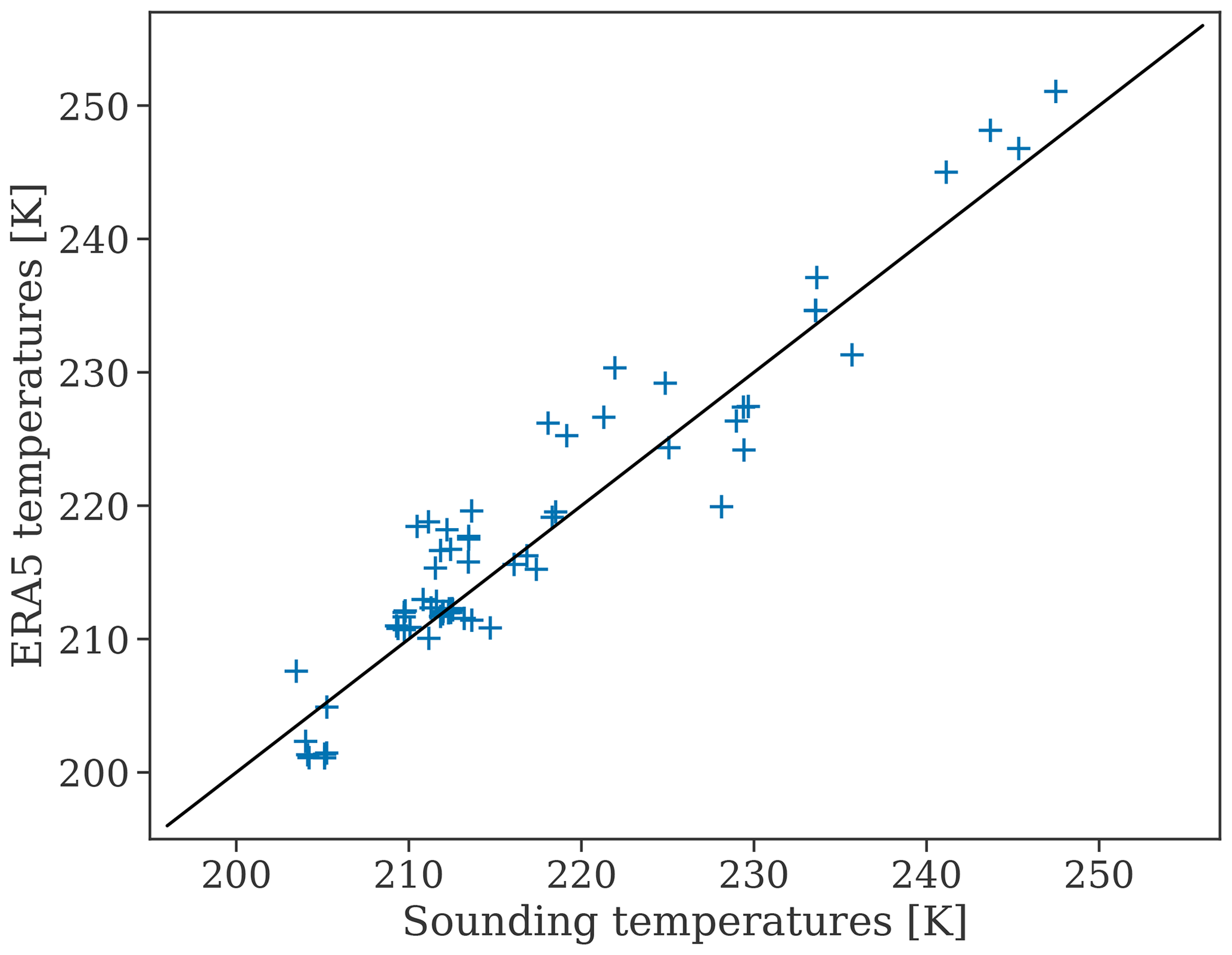
Figure 1 Cloud top temperature extracted from ERA5 scattered against cloud top temperature from the closest available radiosonde release (Andenes) for all detected cirrus clouds between 2015 and 2017. The black one-to-one line indicates exact agreement and shows a slight bias of ERA5 data towards warmer temperatures. The average difference is 1 K.

The available measurement record of observations, including depolarization-sensitive channels, spans from 2011 to the present with a maintenance break from April 2013 to July 2015. The lidar can be operated whenever there is no precipitation and the 10 min average wind speed does not exceed 12 m s⁻¹. The majority of measurements is made during daytime. Possible implications and biases of the measurement routines will be discussed in Sect. 4.

2.2 Spaceborne lidar and radar

We use data from the cloud profiling radar (CPR) aboard CloudSat (Stephens et al., 2002) and the Cloud-Aerosol Lidar with Orthogonal Polarization (CALIOP) aboard the Cloud-Aerosol Lidar and Infrared Pathfinder Satellite Observation (CALIPSO) satellite (Winker et al., 2009). For direct comparison with the ground-based lidar, we use CALIOP Level 1 (1B profile; NASA/LARC/SD/ASDC, 2016) and Level 2 (5 km cloud layer; NASA/LARC/SD/ASDC, 2018) data products for cloud properties such as backscatter, altitude, and optical depth. CALIOP operates on the same wavelengths (1064 and 532 nm) as the lidar at ALOMAR. Here, the vertical resolution in the relevant altitudinal region above 8 km is 60 m, and the horizontal resolution is 1 km. For the phase discrimination between cirrus, mixed-phase, and liquid clouds, we use the 2B-CLDCLASS-LIDAR data product (Sassen et al., 2008), which utilizes the different sensitivities of the radar and lidar to liquid droplets and ice crystals. Beside the cloud phase, we use the cloud top and base height information, and, for each cloudy profile, we retrieve the cloud top temperature from the ECMWF-AUX dataset (version P_R05), which uses ancillary European Centre for Medium-Range Weather Forecasts (ECMWF) state variable data interpolated to each CPR vertical bin.

We are aware that the use of different reanalysis products for temperature retrievals introduces uncertainties. However, as ECMWF-AUX has been specifically designed to provide profiles of temperature from atmospheric reanalysis interpolated on the time and location of the CloudSat/CALIPSO overpass, this makes it the first choice for use in combination with the phase retrieval from the 2B-CLDCLASS-LIDAR product. To draw conclusions about the general CTT distribution of cold clouds without introducing a large bias from the choice of the reanalysis product, we choose a bin size of 2.5 K when showing the distributions in Fig. 7. The choice of 2.5 K is based on previous estimates of the validity of atmospheric reanalysis temperatures in the Arctic: Jakobson et al. (2012) found a bias of up to 2 K for the lowest 890 m when comparing tethersonde data from an Arctic drifting ice station with ERA-Interim reanalysis data. Moreover, Graham et al. (2019) compared ERA5 reanalysis data with radiosondes launched from two ship campaigns in the Fram Strait and found a vertically averaged absolute bias of 0.3 K. Other reanalysis products in their study also showed biases of less than 0.6 K. In addition, our own comparison of the radiosonde data from Andenes with ERA5 data yielded a bias of 1 K. This gives us confidence in the use of different reanalysis products for the spaceborne and ground-based retrievals of the CTT.

Apart from gaps in the satellite dataset (January 2011; January–April 2012; and June, July, and September 2017) we analyze the 2011–2017 period.

2.3 Comparison of ground-based and spaceborne observations

For the statistical analysis, we split the available data from the ground-based lidar into 30 min measurement intervals (shorter measurements also count as one interval), which results in a total number of 1366 measurements between 2011 and 2017. We include all satellite overpasses within a $\mathrm{2}{}^{\circ }\times \mathrm{2}{}^{\circ }$ box around ALOMAR in the analysis. This corresponds to an extent of approximately 80 km in the zonal direction and 220 km in the meridional direction, and it results in 48 873 individual profiles being used for the statistical analysis of cold-cloud properties.

We limit this analysis to single-layer clouds in order to avoid attenuation by the lidar when penetrating multiple cloud layers, which would induce a bias in the statistics due to the opposite upward and downward viewing configurations of the two lidar systems. A cloud scene observed from the ground-based lidar is considered to be multilayer if there is a cloud-free region of at least 200 m vertical distance between two cloudy layers. Otherwise, the scene is regarded as a single-layer cloud.

3 Case study results

To demonstrate the capabilities of the ground-based lidar with respect to observing cold clouds, we present two case studies focusing on (1) a cirrus cloud and (2) a mixed-phase cloud. The cirrus cloud case provides the opportunity to directly compare the ground-based lidar with measurements from the spaceborne CALIOP lidar. For the mixed-phase cloud case, we use the lidar to distinguish between liquid droplets and ice crystals, providing insight into the vertical phase distribution of the cloud.

3.1 Cirrus cloud case

On 1 April 2011, CALIPSO passed over the ALOMAR lidar at 11:11 UTC (13:11 LT) while both lidars were measuring a cloud layer between 9.6 and 11.5 km altitude. The satellite ground track is shown in Fig. 2d, and it crosses the island of Andøya with a horizontal distance to ALOMAR of 2 km northeast of the mountain of Ramnan.

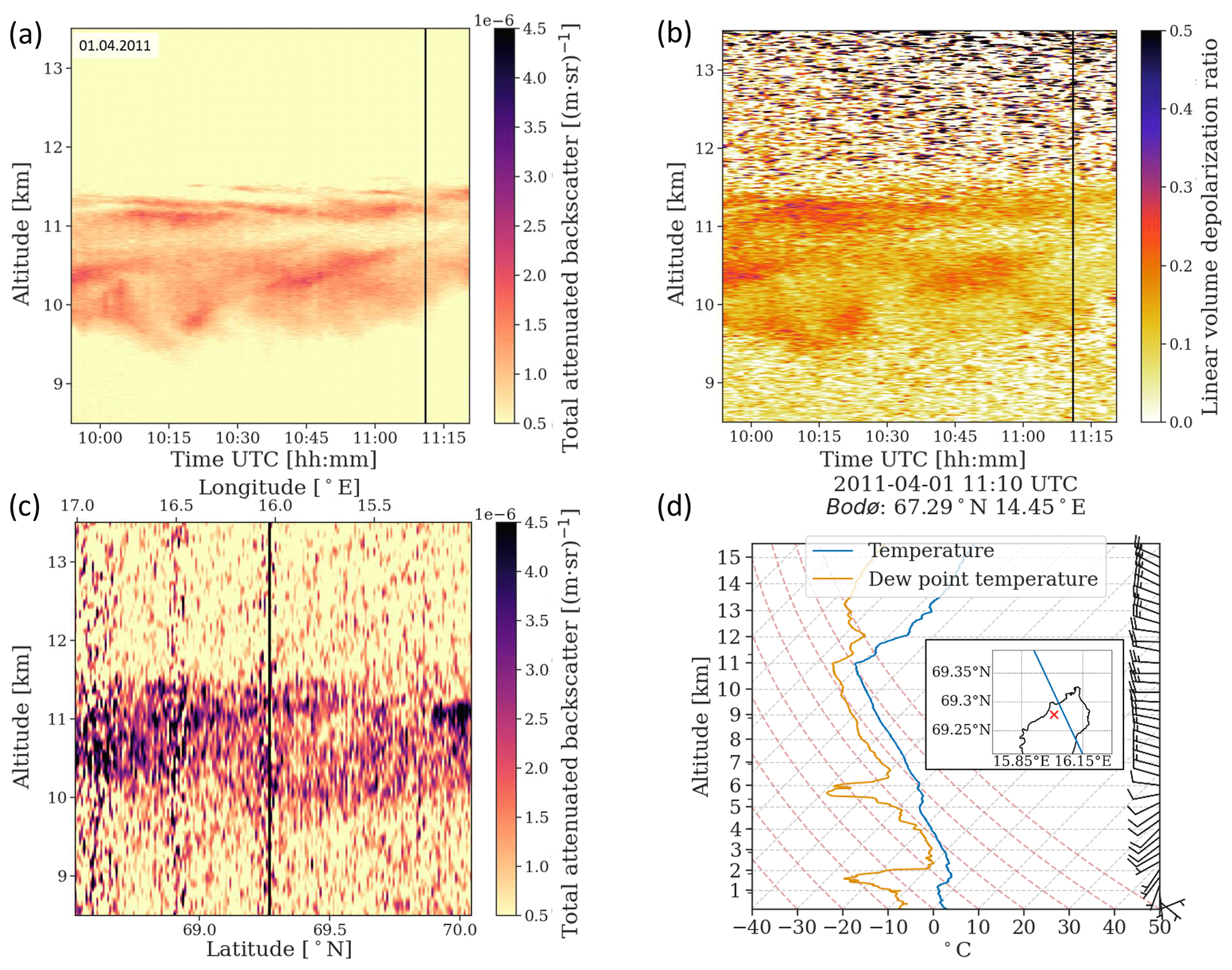
Figure 2 Cirrus cloud measurement on 1 April 2001, showing the total attenuated backscatter at 532 nm from the ALOMAR lidar (a) and CALIOP (c) as well as the linear volume depolarization ratio from the ground-based lidar (b). The closest available radiosounding from Bodø is shown in panel (d), along with a map showing the ground track of the satellite (blue line) and the position of the ground-based lidar (red cross). The black lines show the overpass time in panels (a) and (b) and the closest location during the overpass in panel (c). The vertical and temporal resolutions of the ALOMAR lidar are 7.5 m and 67 s, respectively. The satellite resolution is 60 m in the vertical direction and 1 km in the horizontal direction. In addition, the satellite backscatter is smoothed by a Gaussian filter.

On the same day, the Norwegian west coast was located between a low-pressure system west of Iceland and a high-pressure system centered over Svalbard. The cirrus clouds observed here were located in a region between a warm front in the north, which had passed Andøya the day before, and a vanishing occluded front, which reached from the Atlantic east of Greenland to Southern Norway (Met Office, 2021).

The ground-based lidar was running from 09:53 to 11:20 UTC, followed by a depolarization calibration measurement. From the satellite, we use data from the time when the ground track was located in a geographical box of $\mathrm{2}{}^{\circ }\times \mathrm{2}{}^{\circ }$ in the meridional and zonal direction around ALOMAR. This is the case from 11:11:09 until 11:11:37 UTC (i.e., for a total duration of 28 s).

The total attenuated backscatter from ground- and spaceborne lidar is shown in Fig. 2a and c, respectively. The total attenuated backscatter from the ground-based lidar ranges from $\mathrm{1}\times {\mathrm{10}}^{-\mathrm{6}}$ to $\mathrm{2.5}\times {\mathrm{10}}^{-\mathrm{6}}$ (m sr)⁻¹ in the cloud around the time of the CALIPSO overpass (black vertical line). In terms of vertical structure, the lowest backscatter values inside the cloud are found at around 11 km, and the layer intensifies from there towards both the cloud top and base. From the spaceborne lidar, the total attenuated backscatter ranges between $\mathrm{1}\times {\mathrm{10}}^{-\mathrm{6}}$ and $\mathrm{4}\times {\mathrm{10}}^{-\mathrm{6}}$ (m sr)⁻¹, and the vertical substructure is less clear, although still recognizable, especially at the latitude closest to ALOMAR until around 69.6^∘ N. Here, the retrieved cirrus cloud base and top heights are 9.6 and 11.4 km, respectively. This is in good agreement with the ground-based lidar. Taking temperature data from the closest available radiosonde release into account (from Bodø; 67.28^∘ N, 14.45^∘ E; 11:10 UTC), we see that the temperature at this altitude was −60 ^∘C or lower, i.e., well below the limit for homogeneous freezing (e.g., Heymsfield and Sabin, 1989). According to the World Meteorological Organization, the tropopause is defined as the lowest level at which the lapse rate decreases to 2 K km⁻¹ or less and where the average lapse rate between this level and all higher levels within 2 km does not exceed 2 K km⁻¹ (WMO, 1992). Applying this definition, we estimate the beginning of the tropopause to be located at about 11.0 km (from radiosonde data; see Fig. 2d) or 10.6 km (from reanalysis data) and at a temperature of −70 ^∘C. Thus, the cirrus cloud is extending well into the tropopause, potentially dehumidifying the upper-troposphere–lower-stratosphere region through ice crystal growth and sedimentation (e.g., Kärcher, 2005). However, a quantification of dehydration in this case requires knowledge of further cloud parameters and is beyond the scope of this study.

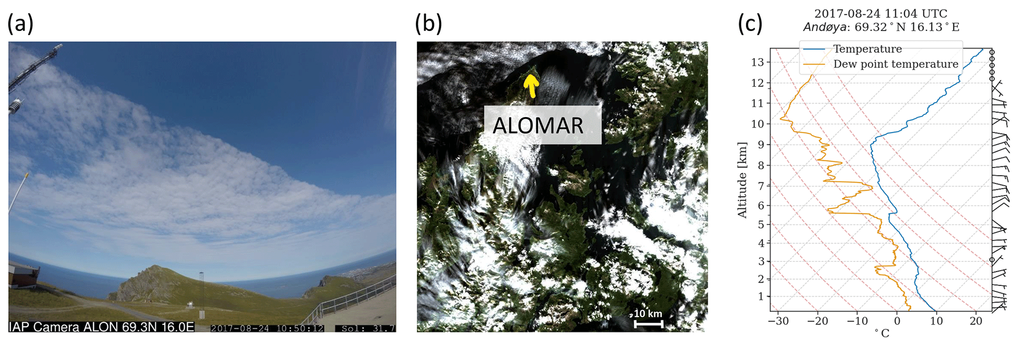
Figure 3 Images of the cloud field probed by lidar at 10:50 UTC, as seen (a) from inside the ALOMAR observatory and (b) from the Sentinel-2 satellite (true color image) (Drusch et al., 2012). In the satellite image, the northern tip of the island is marked by the yellow arrow, and the cloud field probed by the lidar is directly to the north of the island. The border between cloud and clear sky that is visible in both pictures moves through the lidar's field of view at around 10:40 UTC. Temperature, dew point, and wind profiles from a radiosonde released in Andenes at 11:04 UTC on 24 August 2017 are given in panel (c).

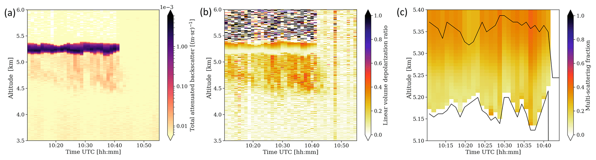
Figure 4 (a) Total attenuated backscatter (TAB), (b) the linear volume depolarization ratio at 532 nm, and (c) the accumulated multiple-scattering fraction inside the liquid cloud body. The black lines indicate the cloud base and top of the liquid cloud body, as identified from the combined parallel and cross-parallel signal. The multiple-scattering fraction is accumulated from cloud base.

The linear volume depolarization ratio from the ground-based lidar is shown in Fig. 2b and ranges from 0.2 to 0.3, indicating thin plate-like particles (shape ratio length / diameter < 0.1) and intermediate and irregular shapes with shape ratios of up to 0.5 (categories I and II in Noel et al., 2002). From the satellite products, the layer-integrated depolarization ratio is available and has values of between 0 and 0.4 over the displayed period (not shown), which covers the range observed by ground-based lidar. A more detailed comparison is not possible, as the noise level of the linear volume depolarization ratio from the satellite is too high.

To compare the cloud optical depths (τ) retrieved from both platforms, we estimated the backscatter-to-extinction ratio to be k=0.2, which yields the best agreement with molecular backscatter above the cloud. Averaging over the time interval from 09:55 to 11:20 UTC, the ground-based lidar gives an optical depth τ of 0.07±0.02. At the location where the satellite ground track has the shortest distance to ALOMAR, the spaceborne lidar retrieves the same value of $\mathit{\tau }=\mathrm{0.07}\pm \mathrm{0.02}$. Thus, the retrieved cloud optical depths show a very good agreement. The observed cloud is an optically thin cirrus cloud according to the classification by Sassen and Cho (1992) ($\mathrm{0.03}<\mathit{\tau }<\mathrm{0.3}$). This is also the most common cirrus category observed at Ny-Ålesund, Svalbard, with a 73 % occurrence (Nakoudi et al., 2021a), and at the subarctic site of Kuopio, Finland (62.74^∘ N, 27.54^∘ E), with a 71 % occurrence (Voudouri et al., 2020).

3.2 Mixed-phase cloud case

The second case that is selected for detailed analysis is an altocumulus mixed-phase cloud, as shown in the image in Fig. 3a. It was observed on 24 August 2017 from 10:10 to 10:40 UTC and was located at 5.2 to 5.4 km altitude. The general weather situation in Northern Norway that day was influenced by two high-pressure systems, one located over Greenland and the other over the Barents Sea extending over the Atlantic towards Iceland. At the same time, two low-pressure systems were located northwest of the British Isles and close to St Petersburg, Russia (Met Office, 2021). This synoptic situation resulted in fields of scattered clouds along the Norwegian coast, mostly of orographic origin over land (see Fig. 3b).

The radio sounding closest in time to the observation was released from Andenes at 11:04 UTC (i.e., ca. 25 min after the end of the cloud observation). Therefore, it did not penetrate the cloud but rather the air mass behind it. The pronounced cloud boundary can be seen in Fig. 3a. Nevertheless, the sounding profile reveals a temperature of −24 to −26 ^∘C in the relevant altitudinal region (Fig. 3c). It increases 2 K right above 5.6 km, at the same altitude where the dew point temperature drops more than 10 K. This indicates a sudden decrease in humidity and marks the border between two air masses: the lower air mass is connected to the cloud, and the upper air mass is warmer and dry above the cloud top.

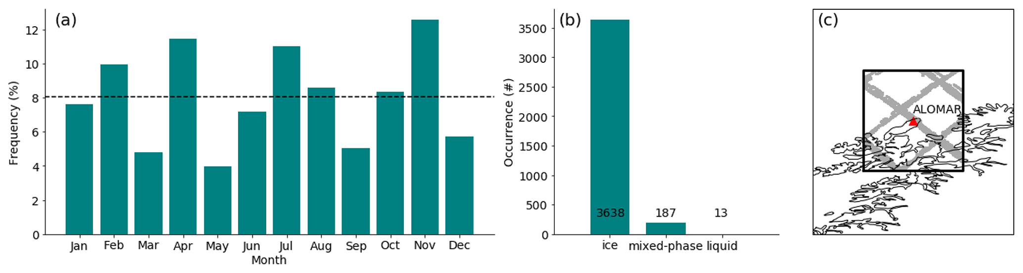
Figure 5 (a) Monthly single-layer cold-cloud occurrence from satellite. (b) The distribution of cloud phase, given as the number of observed single-layer cold clouds. (c) The spatial box from which cloud measurements are taken for the analysis: the ground-based lidar at ALOMAR is indicated by the red triangle, the box extends 2^∘ around ALOMAR (1^∘ in each direction), and satellite overpasses with cloud detection are indicated in gray.

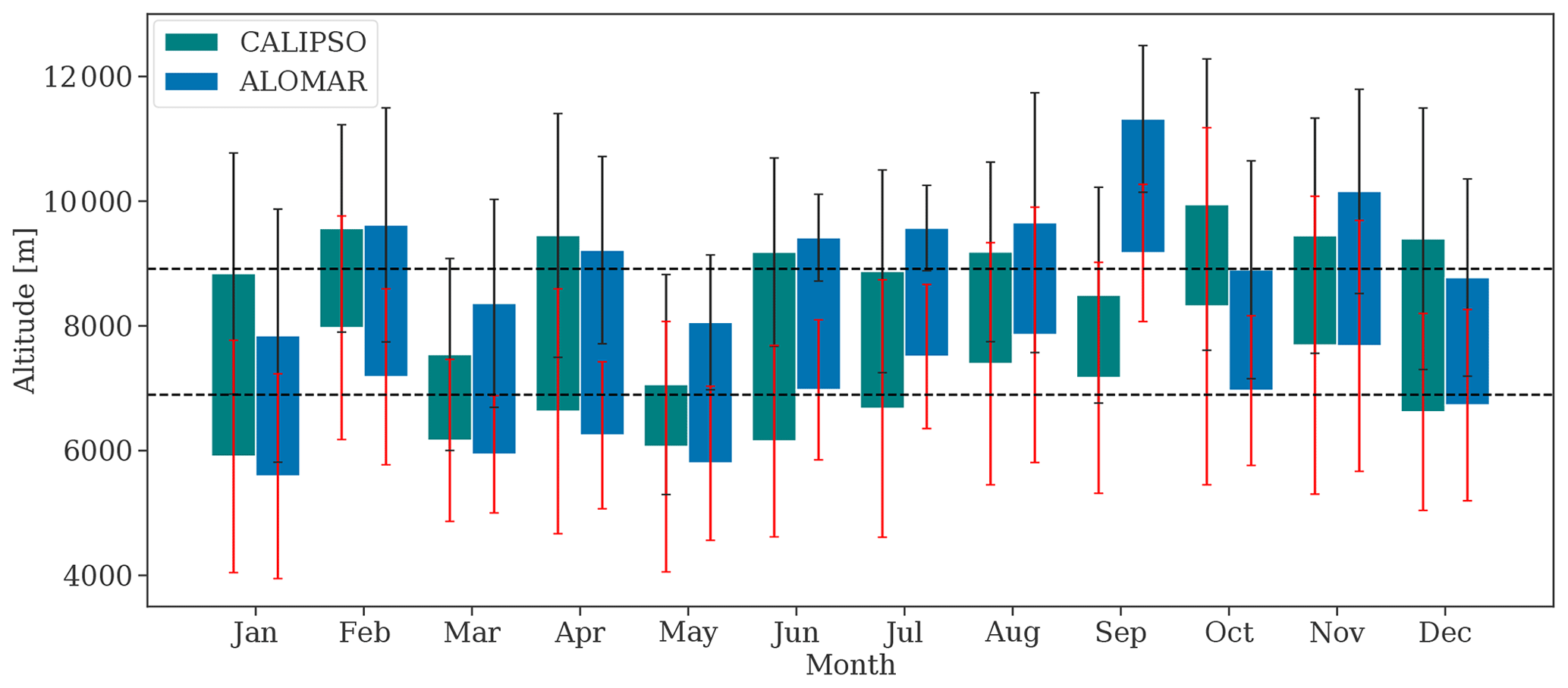
Figure 6 Monthly mean thickness of cirrus clouds observed from the ground-based lidar at ALOMAR (blue) and CALIOP (green). The error bars indicate the standard deviation of the computed cloud top and base heights. The dashed black lines show the multiyear annual average.

The total attenuated backscatter and the linear volume depolarization ratio from the ground-based lidar are shown in Fig. 4. From the backscatter signal, the distinct cloud boundaries at 5.2 and 5.4 km altitude with falling hydrometeors below become apparent. Differences in the linear volume depolarization ratio imply different shapes of the cloud particles (Noel et al., 2002), at least as long as single scattering is concerned. Hexagonal ice crystals typically lead to linear depolarization ratios of 0.2–0.5, depending on the aspect ratio, whereas single scattering from spherical water droplets does not induce any polarization change. The depolarization ratio in the mixed-phase cloud case shows a clear separation into three regions (see Fig. 4b): the center of the cloud around 5.2–5.3 km, with values below 0.1, can be clearly separated from the cloud top and a large area below that extends down to 4.5 km (both with values up to 0.4). Thus, spherical liquid water droplets dominate in the region around 5.2 km, with δ<0.1, whereas the high depolarization values between 4.5 and 5.2 km altitude can be attributed to falling ice crystals (virga). The increasing depolarization ratio from the liquid cloud base towards the cloud top can be attributed to multiple scattering by liquid water droplets, as the cloud is optically thick, meaning that there is no signal coming back from above the cloud. Hu et al. (2006) presented a relationship between the accumulated multiple-scattering fraction in water clouds and the accumulated depolarization ratio δ_acc. We retrieve the altitude of the (assumed) liquid cloud base and top from the gradient in the attenuated backscatter signal, and we use this cloud base as a starting point for the accumulated depolarization and multiple-scattering ratios. Applying the formula $A_{\mathrm{S}}=\mathrm{0.999}-\mathrm{3.906}{\mathit{\delta }}_{\mathrm{acc}}+\mathrm{6.263}{\mathit{\delta }}_{\mathrm{acc}}^{\mathrm{2}}-\mathrm{3.554}{\mathit{\delta }}_{\mathrm{acc}}^{\mathrm{3}}$ from Hu et al. (2006) results in the profile of the multiple-scattering fraction within the cloud, as shown in Fig. 4c. The fraction of multiple scattering increases from around 15 % at cloud base to up to 40 % at cloud top. Note that this calculation assumes that the depolarization signal is entirely explained by multiple scattering from spherical water droplets. Hence, the multiple-scattering fraction of 15 % at cloud base indicates an additional influence from ice crystals within the predominantly liquid cloud layer. This is typical for a liquid-topped mixed-phase cloud, where small ice crystals are formed at the cloud top and then fall through the liquid part of the cloud. The observed structure is in accordance with, for example, in situ observations from aircraft by Barrett et al. (2020) and ground-based lidar observations by Engelmann et al. (2021). These studies found ice production within the supercooled layer at temperatures of −30 and −28.5 ^∘C, respectively, and ice virgae below. Thus, we conclude that there are active ice-nucleating particles at temperatures around −25 ^∘C, although in insufficient amounts for complete glaciation of the cloud.

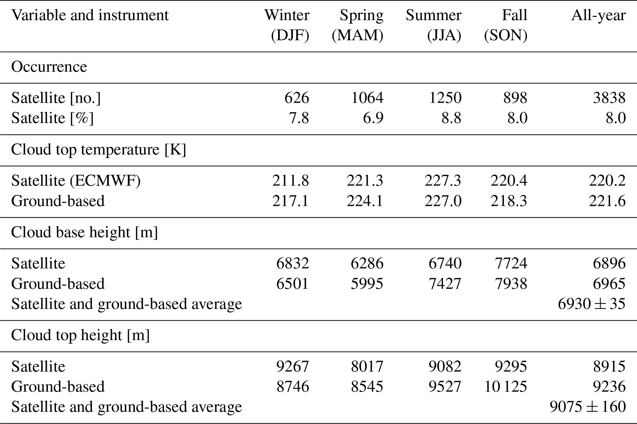
Table 1 The seasonal and multiyear annual (“All-year”) average of occurrence, temperature, and cloud height for the two datasets from the ground- and satellite-based lidar. The occurrence for the satellite is the total number of detections between 2011 and 2017 during the respective season.

4 Cold-cloud statistics

The statistical analysis of cold-cloud properties uses all data from the ground-based lidar at ALOMAR spanning from the installation of the depolarization channel in 2011 until 2017 as well as spaceborne lidar data for the same period.

We define cirrus clouds as all single-layer clouds with cloud base heights between 4000 and 12 000 m and a cloud top temperature below −20 ^∘C (253.15 K). This is based on Sassen et al. (2008) and Heymsfield et al. (2017), who showed, using satellite observations, that cirrus clouds in the Arctic are mostly limited to an altitude range between 4 and 12 km.

To test this definition, we applied it to all 25 779 single-layer clouds detected by CloudSat/CALIPSO during the study period. Of these, 3838 clouds were identified as cirrus clouds. Figure 5c shows the location of these cirrus cloud profiles within the $\mathrm{2}{}^{\circ }\times \mathrm{2}{}^{\circ }$ box around ALOMAR. Using the additional phase information, we find that 95 % of these clouds were indeed pure ice clouds (3638 cases; see Fig. 5b). The remaining 5 % consisted of mixed-phase clouds (187 cases) and pure liquid clouds (13 cases). This confirms that the cirrus cloud definition captures mostly pure ice clouds; however, it cannot be ruled out that some of the cirrus cloud cases identified by the ground-based lidar might include some mixed-phase clouds. A further phase discrimination from the ground-based lidar for this possible mixed-phase cloud influence is beyond the scope of this study. Due to this slight ambiguity, we hereafter refer to these predominantly ice clouds as cold clouds. Furthermore, we conclude that INP concentrations are generally high enough to glaciate single-layer clouds at temperatures below −20 ^∘C.

As can be seen from Fig. 5a, the monthly occurrence of single-layer cold clouds varied between 4 % and 13 %, showing no clear seasonal dependence. On average, 8 % of all satellite profiles were identified as single-layer cold clouds. With a total occurrence of 51 % for single-layer clouds of all heights and phase compositions, this corresponds to 15.4 % of all single-layer clouds being cold clouds according to our definition. This fraction of 15.4 % is less than the 1 : 4 ratio reported by Nomokonova et al. (2019) for Ny-Ålesund, Svalbard (36 % total occurrence of single-layer clouds, thereof 9 % pure ice clouds). The number of cirrus cloud observations from the ground-based lidar also shows no seasonal trend. However, the ground-based record is not continuous due to the hours of operation and weather limitations: measurements are not possible in the case of precipitation or when average wind speeds exceed 13 m s⁻¹ due to local instrument safety restrictions. Thus, the cold-cloud occurrence as seen from the ground-based lidar has a bias towards higher values, and it is not shown here because it cannot be compared to the spaceborne lidar.

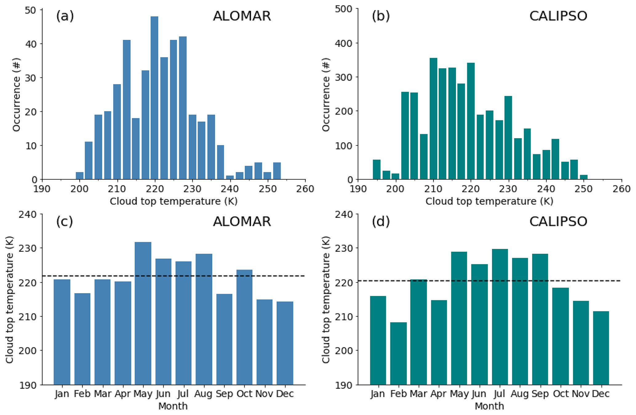
Figure 7 (a, b) Histogram of cloud top temperatures for all cirrus detections from (a) the ground-based lidar and (b) the spaceborne lidar between 2011 and 2017. The bin width is 2.5 K. For the ground-based lidar, the temperatures are interpolated from reanalysis data (ERA5) on pressure levels until 2014 and taken from radiosondes thereafter. (c, d) Monthly average cloud top temperature from (c) ground-based and (d) spaceborne lidar.

Nevertheless, the macroscopic cold-cloud properties (cloud top and base height) for both the ground-based and satellite observations can be compared, and they are displayed in Fig. 6. The corresponding seasonal averages can be found in Table 1. The ground-based lidar records cloud top heights between 5045 and 13 130 m (mean of 9240 m) and cloud base heights between 4040 and 11 090 m (mean of 6970 m) with a pronounced annual cycle. There are distinct increases in height from January to February, from May to June, and from August to September as well as decreases from February to March and from September to October. In general, there is a trend towards higher cold clouds in summer and fall compared with winter and spring. The highest monthly average altitudes (both cloud base and top) are recorded in September, whereas the lowest monthly average altitudes are seen in January. The general trend of higher cold clouds in fall than in winter and spring is also apparent in the results from the spaceborne observations (see Fig. 6). However, the monthly variability is less pronounced than for the ground-based measurements, indicating an influence of the irregular observation times on the ground-based lidar. Cloud top heights as retrieved from the satellite are also slightly lower (4150–12 490 m, mean of 8915 m) than for the ground-based lidar. The cloud base height from satellite varies between 4030 and 11 890 m (mean of 6895 m), which is more similar to the ground-based observations. However, this is expected due to the cloud-type detection algorithm being dependent on the cloud base height. The large standard deviations for cloud top and base heights (as visible in Fig. 6) indicate a larger case-to-case variability than monthly variability for both platforms. Moreover, the average vertical extents of the cold clouds are similar: 2270 m for ground-based measurements and 2020 m for spaceborne measurements.

We show histograms and the monthly averages of the cloud top temperatures from both lidars in Fig. 7. The distributions of observed cloud top temperatures are similar from both platforms: the registered cold clouds showed CTTs between 201 and 253 K (ground-based) and between 196 and 252 K (spaceborne) with a pronounced maximum of cold-cloud occurrence at around 220 K (ground-based) and 210 K (satellite). The distribution from ground-based lidar has a second (lower) maximum at 212 K, closer to the maximum observed from the satellite. Likewise, the second highest peak in the distribution from satellite measurements at 220 K corresponds to the maximum of the ground-based distribution. The main difference between both distributions is the total number of measurements, which leads to the more patchy histogram for the ground-based observations, especially towards the high-temperature end of the distribution. Furthermore, the observed cold-cloud CTTs show a similar annual cycle from both platforms (see Fig. 7c and d). The highest CTTs were registered in summer (between May and August), with values of up to 230 K, whereas CTTs are lowest in the winter months (214 K in December for ground-based measurements and 208 K in February for spaceborne measurements). For the satellite measurements, this low CTT in February coincides with the high mean cloud top height (CTH) in February (see Fig. 6). However, even though the cold clouds in December show the coldest CTTs from the ground-based lidar, their corresponding CTH is not the highest throughout the year. This can partly be explained by the lower temperatures throughout the troposphere in the winter. However, similarly low CTTs in September correspond well to the highest CTHs registered in that month (see Fig. 6).

5 Discussion

First, we put our results into the context of long-term ground-based observations of clouds in the Arctic, and we then compare them to spaceborne instrument studies. The multiyear annual average total cloud occurrence at 4 km altitude varies between around 15 % (Utqiagvik, Alaska) and 30 % (SHEBA, ship-based observatory in the western Arctic Ocean) and decreases with altitude to less than 1 % above 10 km altitude (Shupe, 2011). These values are higher than our finding of 8 % cold-cloud occurrence, and the difference can be explained by the restriction to single-layer clouds (Shupe, 2011, also accounted for multilayer clouds). On the other hand, our result is still larger than the annual mean cirrus occurrence of 2.7±1.8 % reported from Ny-Ålesund by Nakoudi et al. (2021a); this is meaningful, as, according to the authors, their value is negatively biased due to the very strict criteria for reliable detection. Nakoudi et al. (2021a) also find a mean thickness of 2 km and higher cloud bases during summer and fall than during winter and spring. Relatively large variations in geometrical thickness with a tendency towards thicker layers in winter seem to be common in the Northern Hemisphere high latitudes (Nakoudi et al., 2021a; Devasthale et al., 2011).

In the following, we compare our results for cold-cloud occurrence with the earlier estimates of cirrus cloud frequency at high latitudes from CALIPSO and CloudSat by Mace et al. (2009), Nazaryan et al. (2008), and Gasparini et al. (2018). The analyses by Mace et al. (2009) and Nazaryan et al. (2008) are restricted to the first year of observations from CALIPSO and CloudSat. However, whereas Mace et al. (2009) address hydrometeor layers of all altitudes and compositions, Nazaryan et al. (2008) focus on cirrus clouds. They find values of cirrus cloud occurrence of less than 20 % to nearly 30 %, depending on the season and how multilayer clouds are treated in the analysis. These occurrences are more than double the satellite values presented in our study. Nevertheless, it is important to note that all of these studies include observations with multiple layers. For the “single-layer” statistics in Nazaryan et al. (2008), only the top cloud layer is considered, whereas only single-layer observations are considered in our study.

6 Conclusions

We use the record of the tropospheric lidar at the ALOMAR observatory on Andøya in the Norwegian Arctic to retrieve macroscopic (cloud top and base height) and microphysical cloud properties. In analyzing (1) a cirrus cloud and (2) a mixed-phase cloud case, we demonstrate the capabilities of the ground-based lidar with respect to observing cold-cloud properties. Co-located observations from the spaceborne lidar aboard CALIPSO allow for a direct comparison of both lidars for the cirrus cloud case. We then compare the statistics of cold-cloud properties in the Norwegian Arctic as observed from the ground-based and spaceborne instruments between 2011 and 2017. To this end, we define cold clouds as all single-layer clouds with cloud base heights between 4000 and 12 000 m and a cloud top temperature below −20 ^∘C. Applying this definition to the satellite profiles, we find that 95% of these clouds were pure ice clouds. This result suggests that ice formation via homogeneous freezing or (at temperatures above −38 ^∘C) heterogeneous freezing via ice-nucleating particles is mostly sufficient to completely glaciate single-layer clouds at the given temperatures.

The main conclusions of this work are as follows:

1. Observations of an optically thin cirrus cloud agree well between ground-based and spaceborne lidar instruments in terms of the cloud height and optical depth. Cloud height deviations are on the order of 100 m or less, and the difference in the retrieved optical depth is below 10 %.

2. Polarization-sensitive measurements in combination with multiple-scattering considerations from the ground-based lidar can be used to determine cloud structure and vertical phase composition, as demonstrated for a mixed-phase altocumulus cloud.

3. Between 2011 and 2017, 8 % of all satellite profiles were identified as single-layer cold clouds on average (corresponding to 15.4 % of all single-layer clouds). Their average thickness was 2.0 km. No clear seasonal cycle for the cold-cloud occurrence could be identified from the satellite measurements.

4. The ground-based lidar records mean cold-cloud top and base heights of 9.2 and 7.0 km, respectively, with a trend towards higher clouds in summer and fall compared with winter and spring. The mean cold-cloud top and base heights as retrieved from the spaceborne lidar are 8.9 and 6.9 km and are, thus, slightly lower than those from the ground-based lidar. The seasonal variability in cloud thickness and height is smaller than the case-to-case variability.

5. Cold clouds in the Norwegian Arctic are between 1 and 2 km higher in fall than in spring on average, while winter and summer show intermediate values. This is confirmed by both ground-based and spaceborne observations.

6. For both platforms, the retrieved cloud top temperatures show similar distributions and a good agreement in their annual cycle with warmer CTTs in summer.

7. Cold-cloud properties in the Norwegian Arctic agree well with observations from other Arctic sites. Geometrical properties are very similar to Ny-Ålesund, Svalbard, and occurrence is within the range found at sites in Alaska, Canada, the Arctic Ocean, and Svalbard.

Limitations on the applicability of the lidar for mixed-phase cloud research are mainly connected to the restriction to elastic-scattering channels during daylight measurements. When using a lidar with a single field of view and elastic channels only, a more detailed study of the microphysical processes requires complementary observational data from radiosondes and sensitivity studies with radiative transfer simulations in order to account for multiple-scattering effects.

The ground-based lidar at ALOMAR is still in operation, and its long-term installation provides an opportunity to study changes in cold-cloud properties in the rapidly changing Arctic.