Data assimilation of CrIS NH₃ satellite observations for improving spatiotemporal NH₃ distributions in LOTOS-EUROS

Atmospheric levels of ammonia (NH₃) have substantially increased during the last century, posing a hazard to both human health and environmental quality. The atmospheric budget of NH₃, however, is still highly uncertain due to an overall lack of observations. Satellite observations of atmospheric NH₃ may help us in the current observational and knowledge gaps. Recent observations of the Cross-track Infrared Sounder (CrIS) provide us with daily, global distributions of NH₃. In this study, the CrIS NH₃ product is assimilated into the LOTOS-EUROS chemistry transport model using two different methods aimed at improving the modeled spatiotemporal NH₃ distributions. In the first method NH₃ surface concentrations from CrIS are used to fit spatially varying NH₃ emission time factors to redistribute model input NH₃ emissions over the year. The second method uses the CrIS NH₃ profile to adjust the NH₃ emissions using a local ensemble transform Kalman filter (LETKF) in a top-down approach. The two methods are tested separately and combined, focusing on a region in western Europe (Germany, Belgium and the Netherlands). In this region, the mean CrIS NH₃ total columns were up to a factor 2 higher than the simulated NH₃ columns between 2014 and 2018, which, after assimilating the CrIS NH₃ columns using the LETKF algorithm, led to an increase in the total NH₃ emissions of up to approximately 30 %. Our results illustrate that CrIS NH₃ observations can be used successfully to estimate spatially variable NH₃ time factors and improve NH₃ emission distributions temporally, especially in spring (March to May). Moreover, the use of the CrIS-based NH₃ time factors resulted in an improved comparison with the onset and duration of the NH₃ spring peak observed at observation sites at hourly resolution in the Netherlands. Assimilation of the CrIS NH₃ columns with the LETKF algorithm is mainly advantageous for improving the spatial concentration distribution of the modeled NH₃ fields. Compared to in situ observations, a combination of both methods led to the most significant improvements in modeled monthly NH₃ surface concentration and ${\mathrm{NH}}_{\mathrm{4}}^{+}$ wet deposition fields, illustrating the usefulness of the CrIS NH₃ products to improve the temporal representativity of the model and better constrain the budget in agricultural areas.

1 Introduction

Ammonia (NH₃) is an alkaline gas in the Earth's atmosphere. NH₃ is highly reactive and readily reacts with available acids, forming aerosol components harmful to human health (Pope et al., 2009; Lelieveld et al., 2015; Giannakis et al., 2019) and, directly and indirectly, impacting global climate change (Erisman et al., 2011; Myhre et al., 2013). NH₃ is emitted from a large number of sources, including agriculture; natural nitrogen fixation in oceans and plants; volcanic eruptions; and biomass, industrial and fossil fuel burning (Erisman et al., 2015). Globally, agriculture is the largest source of NH₃. Agricultural emissions of NH₃ consist of, among others, volatilized NH₃ after manure and chemical fertilizer application, livestock housing and grazing, and harvesting of crops. About 40 % of the total global NH₃ emissions follow directly from volatilization of animal manure and chemical fertilizer, a spatially variable process highly controlled by the temperature and acidity of soils (Sutton et al., 2013). In western Europe, for instance, agriculture is an even more dominant source of NH₃ and contributes to 85 %–100 % of all NH₃ emissions (Hertel et al., 2011). After the emitted NH₃ is transported through the atmosphere, it is deposited back to the Earth's surface through the processes of wet and dry deposition. Excess amounts of reactive nitrogen deposition can cause several adverse effects, such as eutrophication in aquatic ecosystems and soil acidification (Erisman et al., 2007) and biodiversity loss in terrestrial ecosystems (Bobbink et al., 2010).

Even though NH₃ at its current levels is an important threat to human health and environmental quality, its atmospheric budget is still very uncertain. NH₃ concentrations are highly variable in space and time and are difficult to reliably measure in situ due to the sticky nature of NH₃ leading to potential adsorption to parts of the measurement devices (von Bobrutzki et al., 2010). Globally, only a few NH₃ measurement networks exist, most of which contain only a small number of locations. Moreover, most measurements are performed at a coarse temporal resolution (weeks to months), while most atmospheric processes occur on much shorter timescales. Due to the lack of dense and precise measurement networks, measures for NH₃ emission controls currently rely mostly on estimates from models, for instance from chemical transport models (CTMs). CTMs simulate atmospheric processes such as emissions, transport, deposition and chemical conversion to estimate the spatial and temporal distribution of atmospheric NH₃. However, these models involve large uncertainties. On the one hand, model assumptions and parameterizations are uncertain due to insufficient or lack of knowledge of some of the processes, for instance, the limited understanding of bidirectional fluxes of NH₃ (Schrader and Brümmer, 2014; Schrader et al., 2018) or the direct effect of meteorology on NH₃ emissions (Sutton et al., 2013). On the other hand, uncertainties stem from the underlying input data and the spatial and temporal variation in emissions. Compared to other air pollutants, NH₃ emission inputs are especially uncertain due to their large spatiotemporal variability resulting from the diverse nature of agricultural sources (Behera et al., 2013). In Europe, the uncertainty of the total annual reported NH₃ emissions on a country level is for instance already estimated to be at least round ∼ 30 % (EEA, 2019). Naturally, NH₃ emissions from individual sources have a much higher uncertainty due to errors related to spatial and temporal distribution. So as to reduce the uncertainty in modeled NH₃ fields from CTMs, it is vital to better understand the spatiotemporal distribution of NH₃ emissions.

With the scarceness of in situ measurements and uncertainties in existing models, the atmospheric NH₃ budget remains among the least known parts of the nitrogen cycle (Erisman et al., 2007). Recent satellite observations of NH₃ in the lower troposphere can help us to fill in both observational and knowledge gaps. Satellite instruments, such as the NASA Tropospheric Emission Spectrometer (TES) (Beer et al., 2008), ESA's Infrared Atmospheric Sounder Interferometers (IASI) (Clarisse et al., 2009), the NASA Atmospheric Infrared Sounder (AIRS) (Warner et al., 2016), the Thermal And Near-infrared Spectrometer for carbon Observation–Fourier Transform Spectrometer (TANSO-FTS) (Someya et al., 2020), and the NASA/NOAA Cross-track Infrared Sounder (CrIS) (Shephard and Cady-Pereira, 2015), provide global observations of atmospheric NH₃. Out of the operational satellites that observe NH₃ with twice-daily global coverage, CrIS is the newest instrument and has the lowest radiometric noise in the spectral region used for NH₃ (Zavyalov et al., 2013). Moreover, CrIS has greater vertical sensitivity to near-surface NH₃ and provides retrievals of the vertical distribution of NH₃ (Shephard et al., 2020).

These atmospheric trace gas measurements with satellites have opened up new ways to study the atmospheric budget. Recently, satellite observations have successfully been used for direct estimates of emissions and lifetimes of various other atmospheric species (e.g., SO₂, NO₂, CO₂) of single anthropogenic or natural point sources (e.g., Fioletov et al., 2015; Nassar et al., 2017) or even multiple sources at a time (Fioletov et al.,2017, Beirle et al., 2019). For NH₃ specifically, multiple studies have reported emissions and atmospheric lifetime estimates either based on satellite data (e.g., Zhu et al., 2013; Whitburn et al., 2015; Van Damme et al., 2018; Zhang et al., 2018; Cao et al., 2020; Evangeliou et al., 2021) or directly estimated from satellite data (e.g., Van Damme et al., 2018; Adams et al., 2019; Dammers et al., 2019). Here, also different forms of model inversions have been used. Overall, these studies indicate an underestimation of both anthropogenic and natural NH₃ emissions in the current emission inventories. In addition to estimating NH₃ emissions, various studies used satellite observations to estimate dry deposition fluxes of NH₃ (Kharol et al., 2018; Van der Graaf et al., 2018; Liu et al., 2020).

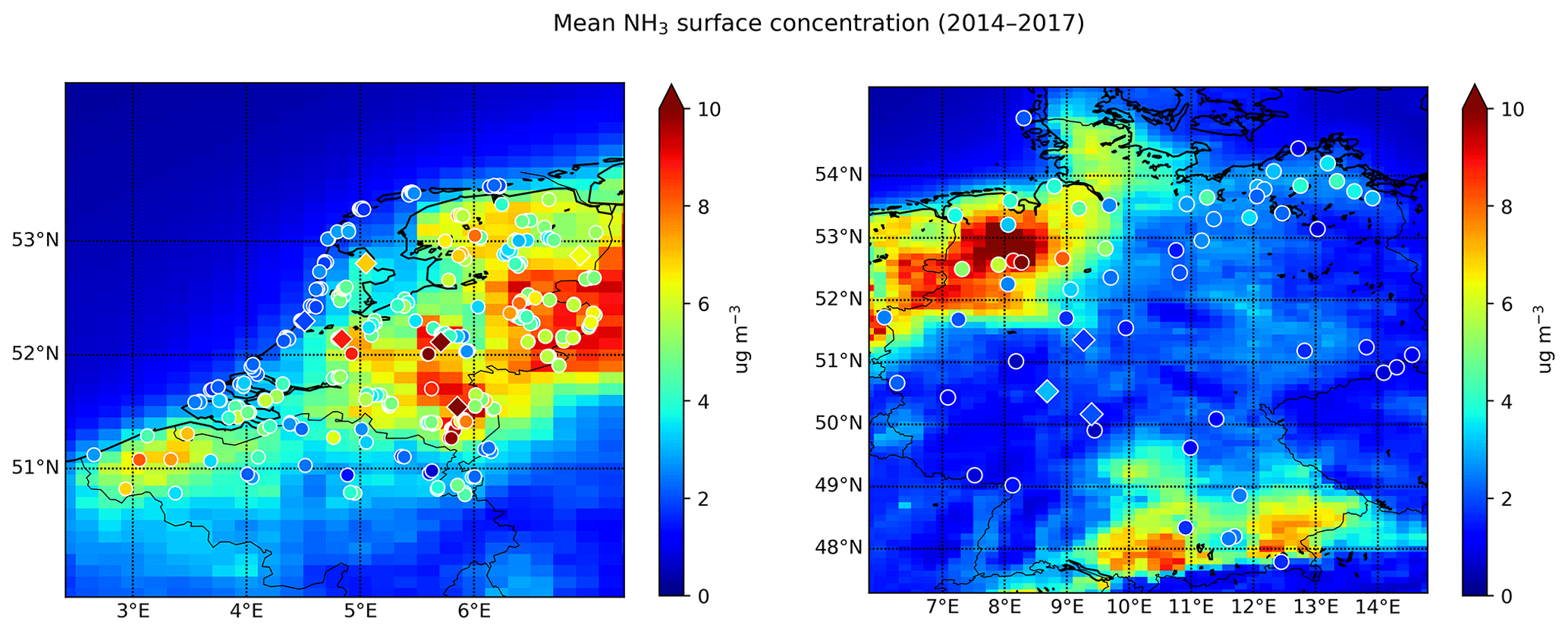
Figure 1 Locations of stations that measure NH₃ surface concentrations. The circles depict passive samplers and the diamonds hourly observations stations.

In this paper, we describe two methods to improve both the temporal and spatial variation of NH₃ emissions in the LOTOS-EUROS chemistry transport model with CrIS NH₃ observations. The first method aims at deriving an improved set of a priori, observation-based NH₃ time factors to be used for the temporal distribution of agricultural emission sources within LOTOS-EUROS. In this method, the NH₃ surface concentrations from CrIS are used to fit daily NH₃ time factors. The second method is used to assimilate the CrIS NH₃ observations into the LOTOS-EUROS model, using a local ensemble transform Kalman filter (LETKF) approach as a data assimilation system. The impact of the two methods, both individually and combined, on the simulated NH₃ emissions, concentration and deposition fields is then evaluated. The focus region of the study is a low-to-high NH₃ emission area within western Europe (the Netherlands, Germany, Belgium), which is representative for other intense agricultural regions in the world. Moreover, the NH₃ emissions within this region are relatively well known, and in situ observations are sufficiently available.

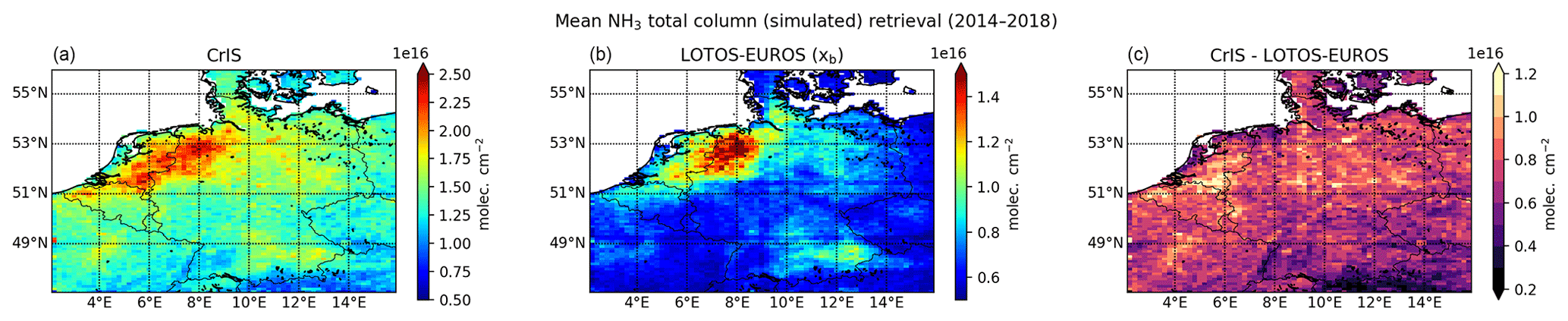
Figure 2 Mean retrieved (a) and simulated (b) NH₃ total column from 2014–2018, as well as their absolute difference (c).

2 Methodology

2.1 LOTOS-EUROS

LOTOS-EUROS is an Eulerian chemistry transport model (Manders et al., 2017) that could be used to simulate trace gas and aerosol concentrations in the lower troposphere. The model has an intermediate complexity with limited run time, allowing ensemble-based simulations and assimilation studies. LOTOS-EUROS uses meteorological data as input, which in this study are taken from the using European Centre for Medium-Range Weather Forecasts (ECMWF). The gas-phase chemistry follows a carbon-bond mechanism (Schaap et al., 2008). The dry deposition fluxes are calculated with the Deposition of Acidifying Compounds (DEPAC) 3.11 module, following the resistance approach, and it includes a calculation of bidirectional NH₃ fluxes (Van Zanten et al., 2010; Wichink Kruit et al., 2012). The wet deposition fluxes are computed using the CAMx (Comprehensive Air Quality Model with Extensions) approach, which includes both in-cloud and below-cloud scavenging (Banzhaf et al., 2012). The anthropogenic emissions are taken from CAMS-REG-AP (Copernicus Atmospheric Monitoring Services Regional Air Pollutants) emissions dataset v2.2 (Granier et al., 2019). For Germany, high-resolution gridded NH₃ emission inputs (GRETA) are used (Schaap et al., 2018). In this study, a region in western Europe (47–56^∘ N, 2–16^∘ E) is modeled, which includes all of Germany, the Netherlands and Belgium (Fig. 2). A spatial resolution of 0.20^∘ longitude by 0.10^∘ latitude is used, corresponding to approximately 12 km by 12 km, which is also roughly the footprint size of CrIS (14 km by 14 km at nadir). The vertical grid extends up to 200 hPa and is split up into 13 vertical layers. This captures the largest part of atmospheric NH₃, as it is a relatively short lived species mainly located in the boundary layer. The interfaces of the vertical layers are based on the pressure layers used in the ECMWF meteorological input data. LOTOS-EUROS is part of the operational Copernicus Atmosphere Monitoring Service (CAMS) ensemble forecasts and analysis for Europe (Marécal et al., 2015). The model has participated in multiple model intercomparison studies (e.g., Bessagnet et al., 2016; Colette et al., 2017; Vivanco et al., 2018), showing overall good performance.

2.2 Datasets

2.2.1 CrIS NH₃

The Cross-track Infrared Sounder (CrIS) is an instrument aboard NASA's sun-synchronous, Earth-orbiting Suomi NPP satellite with an equatorial overpass at 13:30 and 01:30 LST. The CrIS sensor has a spectral resolution of 0.625 cm⁻¹ (Shephard et al., 2015) and a detection limit of 0.3–0.5 ppbv under favorable conditions (Shephard et al., 2020). The instrument has a wide swath of up to 2200 km with pixels of approximately 14 km in size at nadir. Compared to other NH₃ satellite sounders (e.g., AIRS, IASI), CrIS has greater vertical sensitivity of NH₃ close to the surface due to its low spectral noise of approximately 0.04 K at 280 K in the NH₃ spectral region (Zavyalov et al., 2013). Moreover, CrIS has a relatively high near-surface sensitivity and an overpass time around 01:30 LST, which coincides with the time of the day with the highest thermal contrast. The peak sensitivity of the instrument is typically between 900 and 700 hPa, which corresponds to approximately 1 to 3 km (Shephard et al., 2020). The CrIS NH₃ total columns have an estimated total random measurement error of around 10 %–15 % and an estimated random total error of ∼ 30 %. Due to the limited vertical resolution, the NH₃ concentrations at individual retrieval levels have a higher random measurement error of about 10 %–30 % and a total error of ∼ 60 %–100 % (Shephard et al., 2020). Version 1.3 of the CrIS NH₃ product has been evaluated against in situ Fourier transform infrared (FTIR) measurements (Dammers et al., 2017), showing an overall good performance and high correlations of r ∼ 0.8. In this study, we used version 1.5 of the CrIS fast physical retrieval (FPR) NH₃ product, which is based on the optimal estimation method (Rodgers, 2000). More details about the CrIS FPR NH₃ product can be found in Shephard et al. (2020). Here, we used daytime observations of NH₃ (partial) column concentrations and surface concentrations made between January 2014 and December 2018 from the first CrIS sensor, which has the longest observing period. During this 5-year period, a virtually continuous time series of CrIS observations was available. More recent observations were not used due to the technical issues of the CrIS instrument during the summertime in 2019, as well as the potentially anomalous situation resulting from the COVID-19 outbreak in 2020.

2.2.2 In situ observations

Several measurement networks were used to evaluate the simulated concentration and deposition fields. The NH₃ surface concentrations are evaluated against observations from the Dutch Meetnet Ammoniak in Natuurgebieden (MAN) network (Lolkema et al., 2015), the Dutch Landelijk Meetnet Luchtkwaliteit (LML) network (van Zanten et al., 2017), the Belgium Flanders Environment Agency (VMM) network (den Bril et al., 2011) and the German Environment Agency (UBA) network (Schaap et al., 2018). The locations of these sites are shown in Fig. 1. The MAN network provides monthly mean NH₃ surface concentrations since 2005, spread over 80 mostly low NH₃ emission nature areas in the Netherlands. The measurements are performed with low-cost passive samplers from Gradko and have an estimated uncertainty of ∼ 20 % for high concentrations and ∼ 41 % for low concentrations (Lolkema et al., 2015). The NH₃ concentrations in Flanders are measured with passive samplers from Radiello and IVL samplers (den Bril et al., 2011). The LML network observes hourly NH₃ concentrations at six different locations in the Netherlands with different emission regimes (high, moderate, low). Initially, continuous flow denuders from AMOR were used, which have a reported uncertainty of at least 9 % for hourly concentrations (Blank et al., 2001). Around 2016, the AMOR instruments were replaced by miniDOAS instruments (Berkhout et al., 2017), which are active differential optical absorption spectroscopes. For evaluation of the wet deposition fields, observations from wet-only samplers from the Dutch Landelijk Meetnet Regenwatersamenstelling (LMRe) network (van Zanten et al., 2017), whose locations largely overlap with the LML network, and the UBA network (Schaap et al., 2018) are used. The locations of the wet-only samplers are shown in Fig. S1 in the Supplement.

Table 1 Initial parameter guesses and parameter bounds used in the trimodal fit algorithm. Here, doty stands for day of the year.

2.3 Fitting method for deriving CrIS-based NH₃ time factors

A nonlinear least squares method is used to fit a trimodal Gaussian curve to the scaled daily NH₃ surface concentrations (see Sect. 2.3.3) from CrIS in each grid cell. The trust region reflective algorithm is used to perform the minimization (Conn et al., 2000). The minimization algorithm is restrained with initial parameter guesses and bounds for three fitted Gaussians. The three Gaussians represent the spring (μ₁, σ₁ and A₁), autumn (μ₂, σ₂ and A₂) and summer peak (μ₃, σ₃ and A₃) in NH₃ emissions, respectively. The initial parameter guesses are based on the standard MACC-III (Kuenen et al., 2014) NH₃ emission time profiles. The bounds are defined as follows:

• the mean values (${\mathit{\mu }}_{\mathrm{1},\mathrm{2},\mathrm{3}}$) are permitted to shift by 1 month (30 d) to cover the most probable emission peaks;

• the standard deviations (${\mathit{\sigma }}_{\mathrm{1},\mathrm{2},\mathrm{3}}$) are permitted to vary by half their initial value guess (i.e., ± 0.5σ);

• the fitted amplitude of the spring peak (A₁) is allowed to be between 0.1 and 1.0 and amplitudes of the autumn and summer Gaussians (A_2,3) between 0.1 and 0.8.

An overview of the permitted parameter bounds is given in Table 1. The range in permitted $A_{\mathrm{1},\mathrm{2},\mathrm{3}}$ values is quite large, allowing the minimization algorithm to fit meaningful trimodal curves for different types of time-variant NH₃ emission sources simultaneously (e.g., flatter peaks for emissions that are mainly dependent on temperature and specific periods, such as open stables, a sharper more distinct spring, and autumn peaks for emissions following fertilizer or manure application).

After the daily NH₃ time factors are fitted, the diurnal variation from the MACC-III NH₃ time factors is added to obtain hourly time factors. The resulting hourly CrIS-based time factors are used as input for all time-variant NH₃ sources from agriculture subcategories in LOTOS-EUROS; i.e., continuous NH₃ point source emissions remain time-invariant.

2.3.1 Data selection

The CrIS NH₃ concentrations in the lowest retrieval level, i.e., closest to the surface, are used to adjust the daily variability in the hourly profiles spatially on a regular 0.1^∘ by 0.05^∘ grid. First, to collect a sufficient number of observations for the fitting algorithm, the CrIS NH₃ surface concentrations with a quality flag of at least 3 and within a selection radius of 1^∘ around the center points of each grid cell are selected. The daily average NH₃ concentrations throughout the year are computed after application of a simple outlier filter (> 99th percentile excluded given more than three observations). Due to the lower number of observations during winter, and to avoid a bias towards higher values due to lower thermal contrast, observations in January, November and December are ignored. During these months it is anyway prohibited to apply fertilizer or spread manure in parts of the regions (for the Netherlands, see RVO, 2021), and in combination with the colder temperatures, NH₃ concentrations are expected to be low due to low volatilization rates (e.g., Søgaard et al., 2002).

2.3.2 Correction for local-emission-to-concentration ratio

The relationship between NH₃ emissions and surface concentrations differs by region and changes throughout the year due to changes in the meteorological and chemical conditions. To correct for this, the following adjustment factor is applied to the daily CrIS NH₃ surface concentrations. The factor is derived from the NH₃ emission and simulated surface concentration fields from LOTOS-EUROS, which are used to compute the local ratio of the smoothed daily total NH₃ emissions to the NH₃ surface concentrations at the CrIS overpass time per grid cell. These are used as a first-order approximation for the relation between the emission and concentration. The ratios are rescaled by the mean annual values for each grid cell to obtain a unitless daily scaling factor (Fig. S2). After multiplying the daily averaged CrIS NH₃ surface concentrations with this scaling factor, a ± 1σ filter is used to smoothen out the daily time series. To avoid too much flattening of the spring emission peak, a separate filter is applied for the spring period. NH₃ emissions originating from the application of synthetic or manure fertilizers are mainly found during this period, at the beginning of the growing season. This may lead to an increase in observed NH₃ concentrations, which would be filtered out when the same filter is applied for the entire year. Finally, the scaled NH₃ surface concentrations are normalized for each grid cell.

2.4 Data assimilation system

2.4.1 Local ensemble transform Kalman filter

The ensemble Kalman filter (Evensen, 2003) is a sequential data assimilation method that could be used to combine model simulations with observation. In this study, the local ensemble transform Kalman filter (LETKF) formulation is used (Hunt et al., 2007) following the implementation by Shin et al. (2016). The LETKF performs an analysis per grid cell based on nearby observations only, and it is therefore computationally advantageous compared to the regular implementation of the ensemble transform Kalman filter. The basic idea behind an ensemble Kalman filter is to express the probability function of the state in terms of an ensemble with N possible states $x_{\mathrm{1}},x_{\mathrm{2}},\mathrm{\dots }{x}_N$, each considered to be a possible sample out of the distribution of the true state. In this study, the state contains the NH₃ concentrations in a three-dimensional grid and two-dimensional NH₃ emission perturbation factors β. The perturbation factors describe the uncertainty in the emissions and are modeled as samples out of normal distribution with zero mean and standard deviation σ. Spatial variations are initially not defined but are introduced by a localization length scale that is described below. The temporal variation in the emission factors is described by temporal correlation coefficient α, which depends on temporal length scale τ (Lopez-Restrepo et al., 2020; Barbu et al., 2009):

$$\begin{array}{}\text{(1)}& {\mathit{\alpha }}_k=e^{-\mathrm{|}{t}_k-t_{k-\mathrm{1}}\mathrm{|}/\mathit{\tau }}.\end{array}$$

An initial ensemble is created by generating random samples of the perturbation factors. The ensemble is then propagated in time in what is called the forecast step between consecutive analysis times for which observations are available. In the forecast step, the model propagates the analyzed ensemble members from time t_k−1 to time t_k following

$$\begin{array}{}\text{(2)}& x_i\left(k\right)=M_{k-\mathrm{1}}\left(x_i^a\right(k-\mathrm{1}\left)\right),\end{array}$$

where operator M_k−1 describes the model simulation, including application of the perturbation factors that are present in x. The ensemble mean x and forecast error covariance P at time k are expressed as

$$\begin{array}{}\text{(3)}& {\displaystyle }x={\displaystyle \frac{\mathrm{1}}{N}}\sum _{i=\mathrm{1}}^N{x}_i,\text{(4)}& {\displaystyle }\mathbf{P}={\displaystyle \frac{\mathrm{1}}{N-\mathrm{1}}}\sum _{i=\mathrm{1}}^N(x_i-x)(x_i-x{)}^T.\end{array}$$

When CrIS observations (y^CrIS) are available (at time t_k), the LETKF algorithm analyses the ensemble by incorporating the observations to reduce the ensemble spread. The analyzed ensemble members are computed from

$$\begin{array}{}\text{(5)}& {\mathit{x}}_i^a={\mathit{x}}_i+{\mathbf{P}}^{\mathrm{a}}{\mathbf{H}}^T{\mathbf{R}}^{-\mathrm{1}}({\mathit{y}}^{\text{CrIS}}-\mathit{h}({\mathit{x}}_i)+{\mathit{v}}_i).\end{array}$$

Here, h(x_i) represents the simulated retrieval from the state x_i or in particular from the concentration array in x_i. Operator H is a linearization of h(x) to x (see Sect. 2.4.4). The matrix R is the observation representation error covariance, which describes the difference between the simulation and the observation due to measurement and representation errors:

$$\begin{array}{}\text{(6)}& {\mathit{y}}^{\text{CrIS}}-\mathit{h}\left({\mathit{x}}_i\right)\sim N(\mathrm{0},\mathbf{R}).\end{array}$$

The actual implementations of h(x_i), H, and R are described below. The analysis covariance P^a is computed from

$$\begin{array}{}\text{(7)}& {\mathbf{P}}^{\mathrm{a}}={\left[{\mathbf{PH}}^T{\mathbf{R}}^{-\mathrm{1}}\mathbf{H}+\mathbf{I}\right]}^{-\mathrm{1}}\mathbf{P}.\end{array}$$

2.4.2 Observation simulation

The simulated observation vector h(x_i) represents the simulated retrieval, which is what the satellite observes from concentrations described in three-dimensional grid cell x_i, and is computed from

$$\begin{array}{}\text{(8)}& \mathit{h}\left({\mathit{x}}_i\right)={\mathit{y}}_{\mathrm{a}}-\mathbf{A}{y}_{\mathrm{a}}+\mathbf{AG}{x}_i.\end{array}$$

Here, matrix G, the gridding operator, is applied to horizontally and vertically match the simulated partial NH₃ columns in LOTOS-EUROS with the retrieval CrIS pressure levels. Here, air-mass weighted averaging is used to average the model layers to the retrieval levels. The relationship between the true and the retrieved atmospheric NH₃ profiles, i.e., the vertical sensitivity of the CrIS measurements, is described by averaging kernel A. The full relationship between the true and the observed state is given by ${\mathit{y}}^{\text{true}}=\mathit{h}\left({\mathit{x}}^{\text{true}}\right)+\mathit{v}$, which can be rewritten to (Eq. 9) (Rodgers and Connor, 2003)

$$\begin{array}{}\text{(9)}& {\mathit{y}}^{\text{true}}={\mathit{y}}_{\mathrm{a}}+\mathbf{A}\left(\mathbf{G}{\mathit{x}}^{\text{true}}-{\mathit{y}}_{\mathrm{a}}\right)+\mathit{v},\end{array}$$

with y_a the a priori profile that is part of the CrIS retrieval product. The error v is a sample of the observation representation error taken from a normal distribution that describes the possible differences between simulation and retrieval:

$$\begin{array}{}\text{(10)}& v\sim N(\mathrm{0},\mathbf{R}).\end{array}$$

In this study, R is set to the retrieval error covariance that is part of the CrIS product. The linearized observation operator becomes

$$\begin{array}{}\text{(11)}& \mathbf{H}=\mathbf{AG}.\end{array}$$

2.4.3 Analysis per grid cell

The analysis described above is applied per model grid cell; for the exact implementation we refer to Shin et al. (2016). First, the simulated observation vectors h(x_i) are computed for all ensemble members. For the grid cell to be analyzed, all simulations are collected that are within 3.5ρ distance, where ρ is called the localization length scale as well as the matching actual observations y^CrIS. The state elements corresponding to the grid cell are then analyzed using the collected observations and simulations, where the weight of observations further away is limited using Gaussian correlation that decays with distance and that uses the same correlation length scale ρ that is used for collection.

2.4.4 Observation selection

CrIS observations with the highest-quality flag, QF = 5, were used. These observations have a relatively higher impact because of their low uncertainty. As the assumed vertical NH₃ profile shapes in background areas used in the CrIS retrieval and in LOTOS-EUROS differ, CrIS retrievals with “unpolluted” a priori profiles were filtered out. The original CrIS retrieval is performed in the log domain, and therefore either the averaging kernels A from CrIS need to be linearized or the LOTOS-EUROS profiles need to be transformed to the log domain. Linearization of the kernel is only accurate for higher concentrations, and since this is the case for the selected “polluted” retrievals, this option was found to be suitable.

2.4.5 Parameter calibration

In this study, we used a localization radius of ρ = 15 km, a standard deviation of σ = 0.5 and a temporal correlation length of τ = 3 d. Two experiments were performed to study the effect of ρ, σ and τ in more detail. A description of the experiments can be found in Sect. S1 in the Supplement. A limited ensemble size of N=12 was found to be sufficient to describe the imposed model uncertainty, which is not too complicated due to short lifetime of NH₃ and therefore strong relation between concentrations and nearby emissions.

3 Results

3.1 Direct comparison of NH₃ concentrations from CrIS and LOTOS-EUROS

Before looking at the effects of assimilating the CrIS observations, a direct comparison of the modeled and observed NH₃ column densities was made. The simulated NH₃ concentrations from the default run in LOTOS-EUROS were sampled at the locations of the CrIS observations, and after application of the averaging kernels they were compared with the retrievals. The observed and simulated NH₃ total columns averaged over all years are shown in Fig. 2. Similar maps per year are available in Fig. S3. The general pattern of the NH₃ total column densities matches quite well. For instance, the observed and simulated NH₃ columns are very similar in southwestern Germany and close to the Dutch border. The CrIS NH₃ total columns are generally higher than the simulated NH₃ total columns. This is for instance found in large parts of northeastern Germany, along the Belgium coast and in the south of the Netherlands. Here, the observed NH₃ columns were on average approximately a factor 2 higher than the simulated NH₃ columns. Moreover, the observed NH₃ total columns are consistently higher than the simulated NH₃ columns in background areas, with a bias between the observed and modeled concentrations of approximately ∼ 0.5 × 10¹⁶ molecules cm⁻².

Figure 3 Daily grid-averaged NH₃ emission, colored per month. Here, x_b represents the default background run and x_b,CrIS the background run with CrIS-based NH₃ time factors.

3.2 CrIS-based NH₃ time factors

3.2.1 Effect on NH₃ emissions in LOTOS-EUROS

Following the method described in Sect. 2.3, temporal profiles for the NH₃ have been obtained per grid cell. Compared to the original model, the new time profiles vary spatially. Figure 3 shows a comparison of the daily grid-averaged NH₃ emissions between the default background model run (x_b) and the background run with the CrIS-based NH₃ time factors (x_b,CrIS), using a different color for each month. The default NH₃ time factors from MACC-III provide more intra-annual variation than the CrIS-based NH₃ time factors. The default time factors include a very high peak in spring and much lower peaks during summer and autumn (i.e., $A_{\mathrm{1}}/A_{\mathrm{3}}$ = 4.57, $A_{\mathrm{1}}/A_{\mathrm{2}}$ = 3.70). Figure S4 shows the fitted spring parameters (μ₁, σ₁ and A₁). The NH₃ spring peak present in the CrIS NH₃ surface concentrations is generally lower than the default NH₃ spring peak. In large parts of the model region, the CrIS-observed NH₃ spring peak is subsequently lower and less sharp. Compared to the default NH₃ time factors, the amplitude of the spring peak in the CrIS-based NH₃ time factors is now generally much lower. The amplitude of the spring peak differs almost by a factor 2 on average. As a result, there is a decrease in springtime NH₃ emissions, especially in March and April. The CrIS-based NH₃ time factors, and consequently the NH₃ emissions, are, on the other hand, generally higher later in the year. The NH₃ emissions are on average approximately 50 % higher in summer and the beginning of autumn (June to September) and approximately twice as high in October.

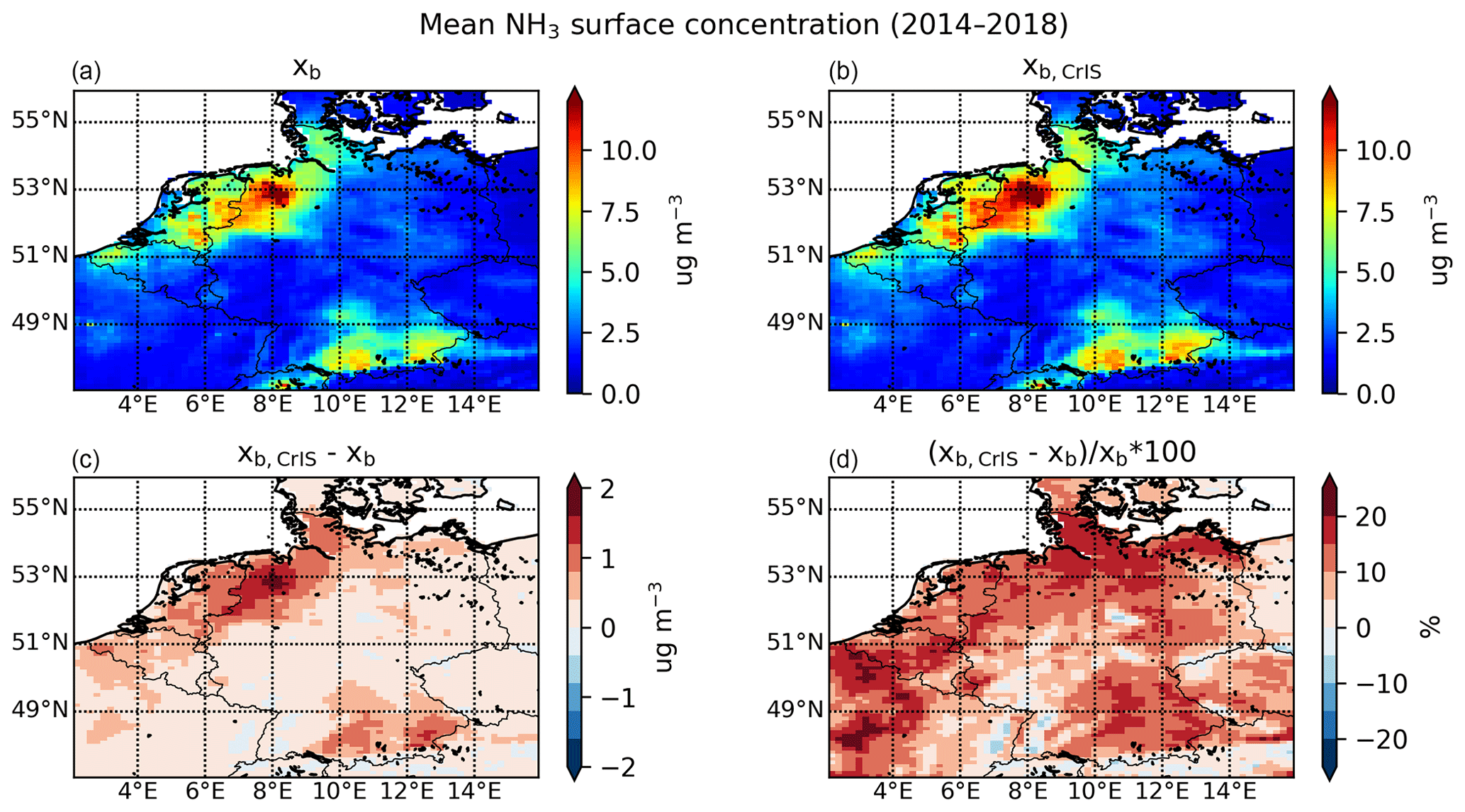
Figure 4 The mean NH₃ surface concentration over 2014 to 2018 from the (a) default background run (x_b) and the (b) background run with CrIS-based NH₃ time factors (x_b,CrIS) and their (c) absolute and (d) relative difference.

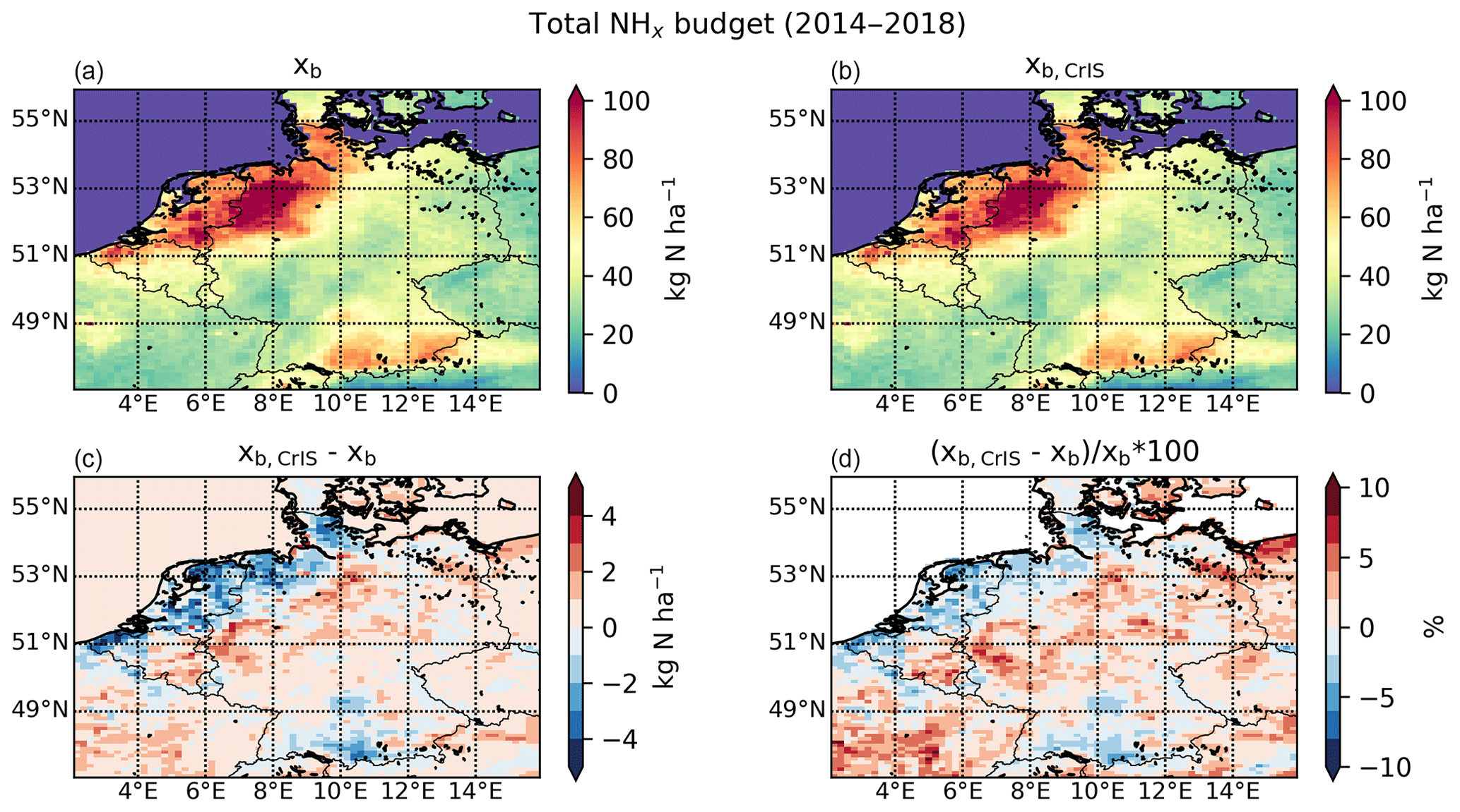
Figure 5 The total NH_x deposition from 2014 to 2018 from the (a) default background run (x_b) and the (b) background run with CrIS-based NH₃ time factors (x_b,CrIS) and their (c) absolute and (d) relative difference.

3.2.2 Effect on NH₃ concentrations and deposition fields in LOTOS-EUROS

The changes in modeled NH₃ surface concentration, total column concentrations and NH_x total deposition from 2014 to 2018 related to the use of the CrIS-based NH₃ time factors alone are shown in Figs. 4, S5 and 5. Here, x_b represents the default background run and x_b,CrIS the background run with the CrIS-based NH₃ time factors. The use of the CrIS-based emission time profiles led to an overall increase in mean NH₃ surface concentrations. The absolute change is largest in areas with already relatively high NH₃ surface concentrations, for instance in northwestern Germany, where the mean NH₃ surface concentrations increased by up to 2 µg/m³. The mean NH₃ surface concentrations increased by up to ∼ 25 % due to the change in NH₃ time factors. The effect of the CrIS-based NH₃ time factors on the NH₃ total column concentrations is smaller, with minor changes from minus ∼ 5 % up to 5 %. The mean NH₃ total column concentrations generally increase in areas with already high NH₃ concentrations, such as large parts of the Netherlands, and decrease in background areas with little NH₃ emissions, for instance in central Germany. The use of the CrIS-based NH₃ time factors led to ∼ 10 % less total NH_x deposition along the northwestern coast, including agricultural hotspots such as the Netherlands and northwestern Germany, and an increase of up to ∼ 10 % in background areas.

Figure S6 compares the daily, grid-averaged, NH₃ surface concentrations, total column concentrations, and NH_x wet and dry deposition, with different colors per month. Here, a similar redistribution is observed for the NH₃ concentration and deposition fields as seen earlier for the NH₃ emission fields. Compared to the default background run (x_b), the NH₃ concentration fields were up to a factor 2 lower during March and April. The NH₃ total columns decreased in spring, with the largest decrease occurring in April (up to ∼ 60 %). The NH₃ surface concentrations increased during the summer and the beginning of autumn – up to ∼ 50 % in September. During these months, a similar but slightly lower increase in the NH₃ total column concentrations is observed.

Because the CrIS-based NH₃ time factors vary per year, the interannual variation in the modeled NH₃ fields is much larger. Figure S7 shows the relative changes in NH₃ surface concentration, total column concentration and NH_x deposition fields per year. Overall, the mean NH₃ surface concentration increases by up to ∼ 30 % per year. The largest increases occurred in 2016 and 2018, which are years with relatively high summer temperatures (Copernicus Climate Change Service, 2021). The variation in the annual mean NH₃ total column concentrations is much smaller (−15 % to +15 %). The relative change in the NH_x budget shows much more variation, with the most prominent increase occurring in 2014 (+25 %) and decreases occurring in 2018 (−25 %).

The temporal redistribution of the NH₃ emissions thus significantly impacts the modeled NH₃ concentration and deposition fields, too. Generally, a part of the initial spring NH₃ emissions is now attributed to the summer and autumn months. Depending on the degree of redistribution, there are distinct changes in the NH_x budget. Looking at the fitted spring peak parameters (Fig. S4) and the matching CrIS-based NH₃ factors at hourly measurement sites (Fig. S8), clear interannual differences are observed. For instance, a relatively sharp spring peak was observed over the Netherlands in 2014. In 2018, on the other hand, the fitted spring peak had a distinctly lower amplitude and started later in the year. Moreover, a relatively large rise in NH₃ time factors was observed again in late summer and autumn (July to September). Compared to 2014, this resulted in a relatively larger redistribution of the NH₃ emissions towards warmer months. The higher temperatures resulted in lower dry deposition velocities and more vertical mixing and transport of NH₃, leading to an overall decrease in NH_x deposition over the Netherlands. Moreover, the summer of 2018 was relatively dry, also leading to higher NH₃ total column concentrations and a decrease in wet NH_x deposition.

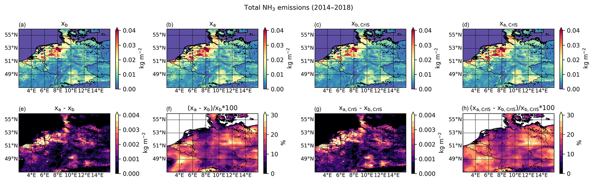
Figure 6 The total NH₃ emissions in 2014–2018 in the background runs x_b and x_b,CrIS and in analysis runs x_a and x_a,CrIS (a–d), as well as their absolute and relative difference (e–h).

3.3 Local ensemble transform Kalman filter

3.3.1 Effect on NH₃ emissions and concentrations in LOTOS-EUROS

The CrIS NH₃ columns were assimilated using the local ensemble transform Kalman filter (LETKF) described in Sect. 2.4. Assimilations were performed either using the default emission time profiles (x_a) or using the CrIS-based profiles (x_a,CrIS). The total NH₃ emissions from 2014 to 2018 and the relative and absolute changes compared to background simulations x_b and x_b,CrIS are shown in Fig. 6. The corresponding mean NH₃ surface and total column concentrations are shown in Figs. S9 and S10. The absolute NH₃ emission updates by the LETKF are, as expected, largest in regions with already high NH₃ emissions. There is a maximum increase of ∼ 30 % in total NH₃ emission by the LETKF over the entire period for some grid cells. Relatively, the largest changes are found in the southern parts of the Netherlands (province of Noord-Brabant), the west coast of Belgium (province of West-Vlaanderen), and the northeastern parts of Germany and France. Compared to the analysis run using default emission time profiles (x_a), the analysis runs with the CrIS-based NH₃ profiles (x_a,CrIS) generally have more NH₃ emission and consequently higher NH₃ surface and total column concentrations. The long-term spatial patterns of the emission updates by the LETKF, however, remained very similar.

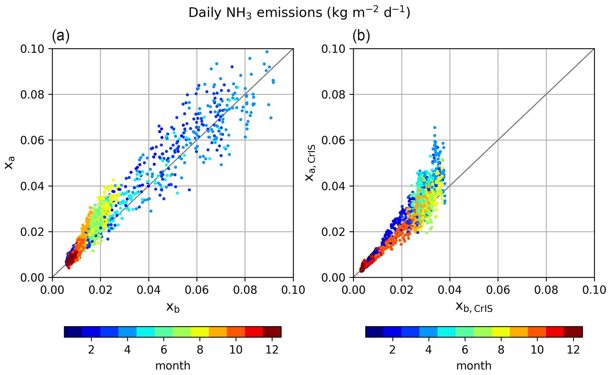
Figure 7 Daily grid-averaged NH₃ emissions in 2014–2018 from the (a) default background run (x_b) versus analysis run (x_a) and from the (b) background run with the CrIS-based NH₃ time factors (x_b,CrIS) versus analysis run x_a,CrIS, colored per month.

To study the effect of the LETKF in more detail, the daily grid-averaged NH₃ emissions of the background runs (x_b and x_b,CrIS) are plotted against analysis runs (x_a and x_a,CrIS) in Fig. 7. Similarly, the NH₃ surface and total column concentrations are plotted in Fig. S11. In the runs with the default NH₃ time factors (x_b and x_a), data assimilation of the CrIS NH₃ columns led to both positive and negative emission updates in spring. In the summer, on the contrary, it mostly resulted in an increase in NH₃ emissions. In the runs with the CrIS-based NH₃ time factors (x_b,CrIS and x_a,CrIS), the pattern is distinctly different. Compared to the default runs, the NH₃ emission updates in spring are now smaller and largely positive, with the largest updates occurring in April. Moreover, the NH₃ emission updates were generally smaller during summer, too. This is related to the fact that the CrIS NH₃ surface concentrations were used to fit the NH₃ time factors, which resulted in the model being closer to the CrIS observations already.

Perturbation factor β is the computed multiplication factor by which the initial input NH₃ emissions are updated in the LETKF. The mean perturbation factors β per year are shown in Fig. S12. The pattern of the NH₃ emission updates does not change drastically between years, which points to a consistent, spatial misdistribution of the emissions in the current inventory. By far the largest mean NH₃ emission updates took place in 2018, followed by 2015.

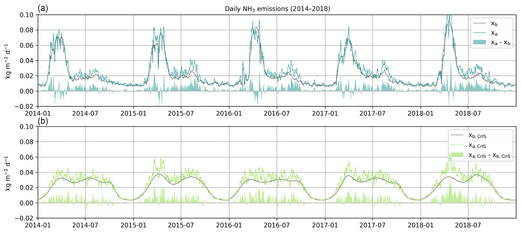
Figure 8 Time series of the daily grid-averaged NH₃ emissions in the background and analysis runs, as well as their absolute difference. Panel (a) (blue) represents the default background (x_b) and analysis run (x_a). Panel (b) (green) represents the background (x_b,CrIS) and analysis run (x_a,CrIS) with the CrIS-based NH₃ time factors.

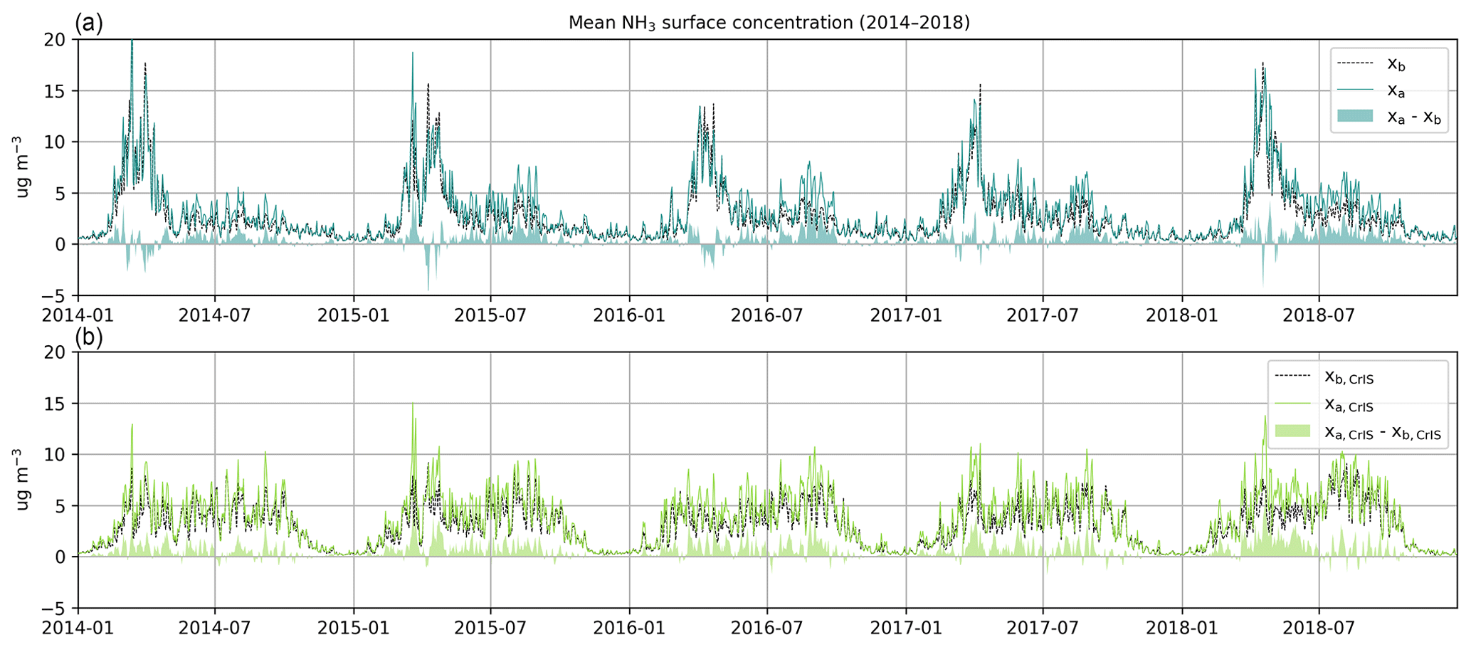
Figure 9 Time series of the daily grid-averaged NH₃ surface concentrations in the background and analysis runs, as well as their absolute difference. Panel (a) (blue) represents the default background (x_b) and analysis run (x_a). Panel (b) (green) represents the background (x_b,CrIS) and analysis run (x_a,CrIS) with the CrIS-based NH₃ time factors.

Figure 8 shows time series of the daily grid-averaged NH₃ emissions in both background runs x_b and x_b,CrIS and analysis runs x_a and x_a,CrIS. Figures 9 and S13 show the corresponding time series and changes in NH₃ surface and total column concentrations. The NH₃ emissions in the default background run (x_b) have a strong, annually reoccurring spring peak. After this peak, the NH₃ emissions decrease steeply and then slightly increase again in late summer and autumn (August and September). In analysis run x_a, the spring NH₃ emissions are both positively and negatively adjusted. Later in the year, almost only positive emission updates are found. The largest positive NH₃ emission updates occurred around August and September, which suggests an underestimation of the autumn NH₃ peak in the default runs.

In the background runs with the CrIS-based NH₃ time factors (x_b,CrIS), the NH₃ emissions are much more evenly distributed over the year. In contrast to the default runs, practically only positive NH₃ emission updates occurred in the analysis run (x_a,CrIS). The largest NH₃ updates took place during spring (March to May). The flattening of the NH₃ emissions led to a flattening in NH₃ concentration fields, too. Compared to default runs (x_b and x_a), there is much less interannual variation in the NH₃ surface and total column concentrations. As a result, the NH₃ concentrations during summer and autumn could be at the same level or even higher than the springtime concentrations. During the warm summer of 2018 (Copernicus Climate Change Service, 2021), for instance, the NH₃ concentrations in August even clearly exceed the spring NH₃ concentrations.

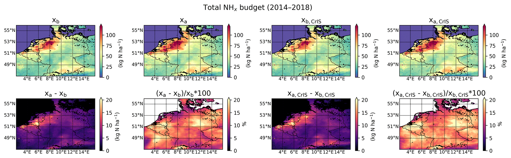
Figure 10 The total NH_x budget from 2014–2018 in the background (x_b and x_b,CrIS) and analysis (x_a and x_a,CrIS) model runs in LOTOS-EUROS, as well as their absolute and relative difference.

3.3.2 Effect on NH_x deposition in LOTOS-EUROS

The modeled total NH_x budgets from 2014 to 2018 from the two background runs (x_b and x_b,CrIS) and analysis runs (x_a and x_a,CrIS) are shown in Fig. 10. Overall, the modeled NH_x budget shows the same spatial pattern as the NH₃ emissions. Like the NH₃ emissions, the relatively largest spatial differences between the background and analysis runs took place in the south of the Netherlands, the west of Belgium and northeast Germany. Compared to the default runs, the relative changes in the total NH_x budget were slightly larger in the runs with the CrIS-based NH₃ time factors (x_b,CrIS and x_a,CrIS).

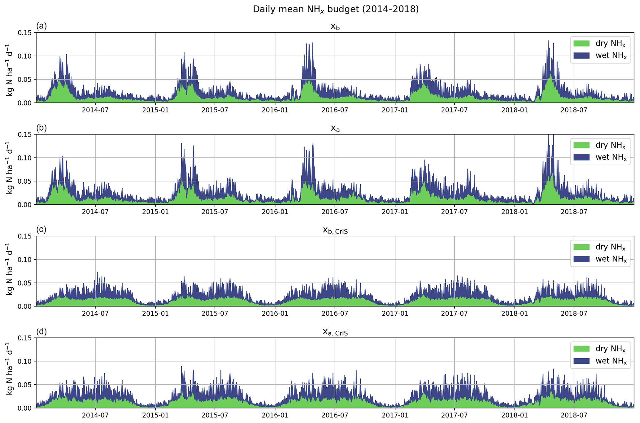
Figure 11 Time series of the average amounts of dry (green) and wet (blue) NH_x deposition in the different model runs. Panels (a) and (b) represent the default background (x_b) and analysis (x_a) run, and panels (c) and (d) represent the background (x_b,CrIS) and analysis (x_a,CrIS) run with the CrIS-based NH₃ time factors.

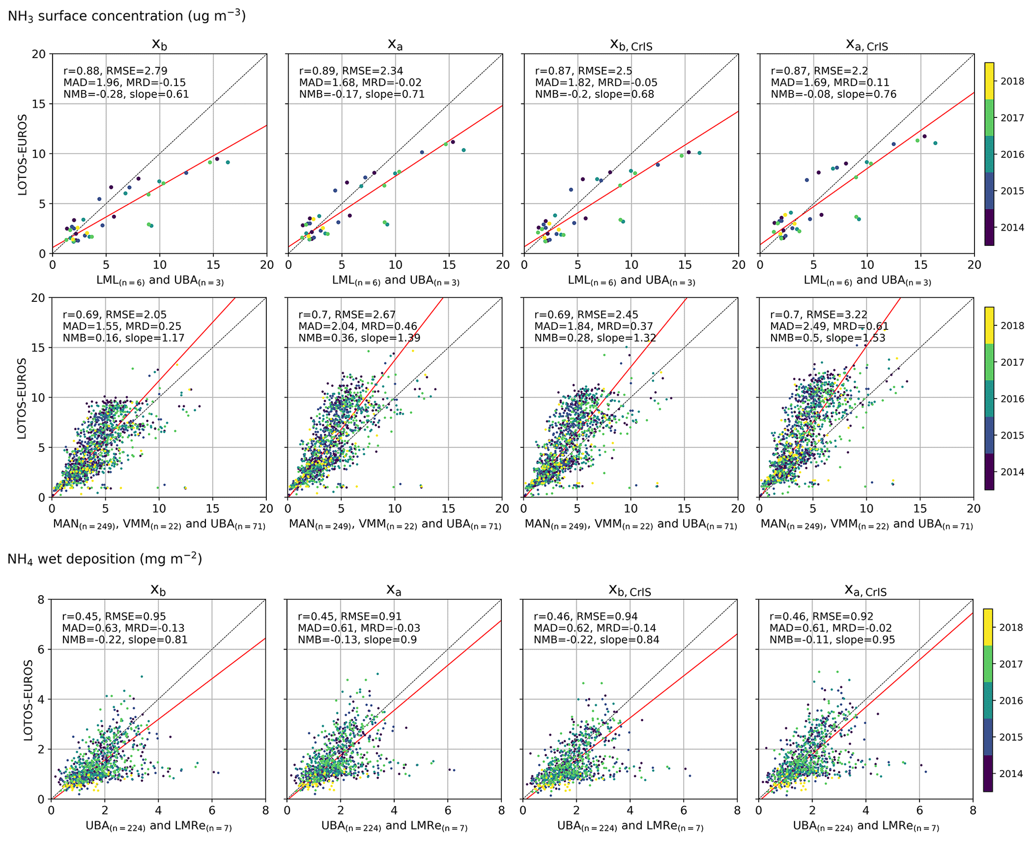
Figure 12 Comparison of the modeled annual average NH₃ surface concentrations and ${\mathrm{NH}}_{\mathrm{4}}^{+}$ wet deposition fields to in situ observations.

The modeled NH_x deposition follows the temporal distribution of the NH₃ emissions, too. Time series of the daily wet and dry deposition amounts in the domain are shown in Fig. 11. The wet and dry deposition in the default runs (x_b and x_b,CrIS) versus the analysis runs (x_a and x_a,CrIS) per month is shown in Fig. S14. In the default background run (x_b), the total NH_x deposition peaks in March and April. In the analysis run (x_a), the dry and wet deposition both increased and decreased during spring (March to May). Later in the year, the wet and dry NH_x deposition mostly increased in the analysis run, particularly in August and September. In the background runs with the CrIS-based NH₃ time factors (x_b,CrIS and x_a,CrIS), the modeled dry and wet deposition fields are much less variable. Following the NH₃ emission updates, both the dry and wet deposition mostly increased in the analysis run, especially in March and April. Moreover, the use of the CrIS-based NH₃ time factors resulted in a redistribution of the ratio of wet and dry deposition over the year. As a result of the relatively lower spring NH₃ surface concentrations, there is a reduction of the dry deposition during spring. The relatively higher summer NH₃ total column concentrations led to a shift in wet deposition, too, from spring to summer.

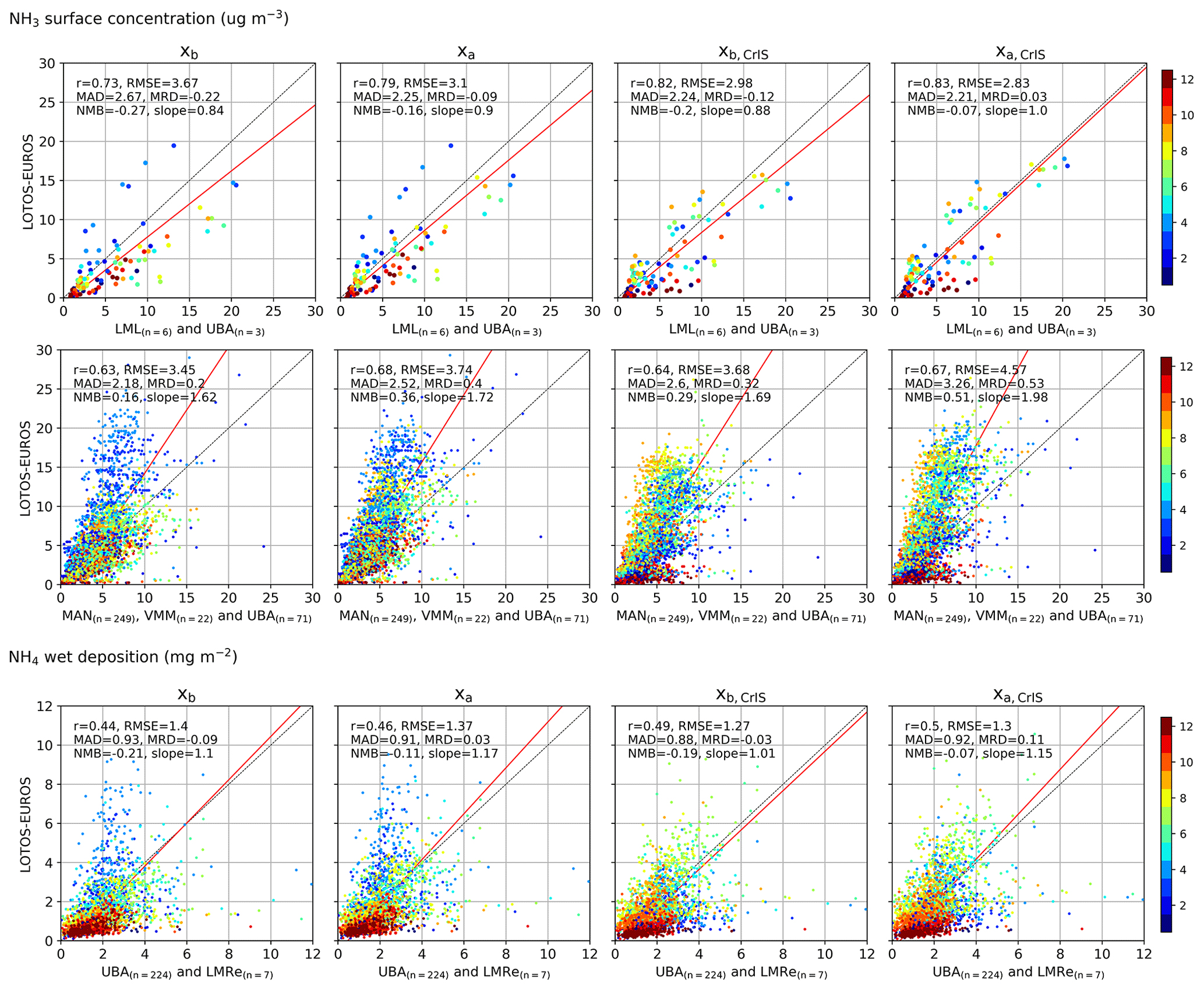
Figure 13 Comparison of the modeled monthly mean NH₃ surface concentrations and ${\mathrm{NH}}_{\mathrm{4}}^{+}$ wet deposition fields to in situ observations. The colors indicate the month.

3.4 Comparison to in situ observations

The modeled NH₃ surface concentration and ${\mathrm{NH}}_{\mathrm{4}}^{+}$ wet deposition fields are compared with in situ observations. First, the spatial distribution is evaluated by comparing the modeled NH₃ surface concentration and ${\mathrm{NH}}_{\mathrm{4}}^{+}$ wet deposition fields to the observed annual averages per measurement site. Second, the temporal distribution is evaluated by comparing the modeled NH₃ surface concentration and ${\mathrm{NH}}_{\mathrm{4}}^{+}$ wet deposition fields to the same set of observations but on a monthly basis. The comparisons are done per type of observation, e.g., all available wet-only measurements simultaneously. To differentiate between different NH₃ emission regimes, the results are plotted separately for either all hourly observations or for the passive samplers. The results are shown in Figs. 12 and 13. The Dutch site with the highest NH₃ surface concentrations, Vredepeel, is excluded from this comparison because of the large model–observation discrepancies here (see Fig. S18). This site is located near agricultural emission sources and therefore is less representative of a larger region. In these figures, the first column shows the comparison for the default background run (x_b), the second column shows the background run with CrIS-based NH₃ time factors (x_b,CrIS), the third column shows the analysis run with the default NH₃ time factors (x_a) and, finally, the fourth column shows the analysis run with CrIS-based NH₃ time factors (x_a,CrIS).

3.4.1 Spatial distribution

Figure 12 shows the scatterplots of the annual averages per site per year. The annual average NH₃ surface concentrations (top row) in the default run x_b show a strong correlation (r = 0.88) with the observed concentrations at the hourly observation sites (LML and UBA). Here, the NH₃ surface concentrations are generally underestimated (slope = 0.61). The annual average NH₃ surface concentrations (middle row) at the passive sampler sites (MAN, VVM and UBA) are generally overestimated (slope = 1.17), with a lower, but still relatively strong, correlation observed (r = 0.69). The modeled annual average ${\mathrm{NH}}_{\mathrm{4}}^{+}$ wet deposition budgets (bottom row) are moderately correlated with the observations from wet-only samplers (r = 0.45) and are generally lower than the observed wet deposition (slope = 0.81). When using the CrIS-based NH₃ time factors, the annual average NH₃ surface concentrations and ${\mathrm{NH}}_{\mathrm{4}}^{+}$ wet deposition budgets are slightly increased. This led to a slight overall increase in slope between all observations and the background run with the CrIS-based NH₃ time factors (x_b,CrIS). As the annual totals, and herewith the spatial distribution of the NH₃ emissions, remained the same in this run; the other measures (correlation coefficient (r), root-mean-square error (RMSE), mean absolute difference (MAD), mean relative difference (MRD), and normalized mean bias (NMB)) did not change drastically on a yearly basis.

The comparison with annual average NH₃ surface concentrations from the passive sampler networks from both analysis runs (x_a and x_a,CrIS) slightly worsened compared to the background runs (x_b and x_b,CrIS). The comparison at the hourly observation and wet-only sampler sites, on the other hand, showed clear improvements. Here, virtually all statistical measures improved, illustrating an overall improvement in modeled NH₃ surface concentration and ${\mathrm{NH}}_{\mathrm{4}}^{+}$ wet deposition field spatially. Of all runs, the analysis run with the CrIS-based NH₃ time factors (x_a,CrIS) compared the best with the hourly observation and wet-only sampler network. The differences between the modeled and observed NH₃ surface concentrations at the hourly observation were distinctly smaller, compared to the default background run (x_b: {RMSE = 2.79, MAD = 1.96, MRD = −0.15, NMB = −0.28} versus x_a,CrIS: {RMSE = 2.2, MAD = 1.69, MRD = −0.11, NMB = −0.08}). Here, also the slope largely improved (x_b: slope = 0.61 versus x_a,CrIS: slope = 0.76). The same is observed for the modeled NH₄ wet deposition fields, where the slope improved particularly (x_b: {RMSE = 0.95, MAD = 0.63, MRD = −0.13, NMB = −0.22, slope = 0.81} versus x_a,CrIS: {RMSE = 0.92, MAD = 0.61, MRD = −0.02, NMB = −0.11, slope = 0.95}).

3.4.2 Temporal distribution

Figure 13 shows the scatterplots of the monthly means per site. The modeled monthly NH₃ surface concentrations from the default background run (x_b) are strongly correlated with the hourly observation network (r = 0.73) and with the passive sampler network (r = 0.63). Both comparisons show a distinct overestimation of the NH₃ surface concentration in March and April. The observed NH₃ surface concentrations at the hourly observation sites are higher than the modeled ones during the rest of the year. At the passive sampler sites, the observed versus modeled monthly NH₃ surface concentrations during the rest of the year lie more around the one-on-one line. Here, too, the modeled NH₃ surface concentrations are slightly underestimated at the beginning of summer (June and July). The ${\mathrm{NH}}_{\mathrm{4}}^{+}$ wet deposition is moderately correlated with monthly observations from wet-only samplers (r = 0.44). At these sites, a similar pattern is observed. The modeled ${\mathrm{NH}}_{\mathrm{4}}^{+}$ wet deposition is overestimated in spring (especially March and April) and underestimated during the rest of the year. In general, this comparison indicates an overestimation of the NH₃ spring peak emissions in the default model runs, particularly in March and April, and an underestimation of the NH₃ emission during the rest of the year, mainly during summer (June, July, August).

The use of the CrIS-based NH₃ time factors (x_b,CrIS) led to an overall improvement at the hourly observation and wet-only sampler sites. Compared to the default background run (x_b), higher correlations and lower differences (RMSE, MAD, MRD, NMB) are observed. At the hourly observation sites, the comparison improved the most (x_b: {r = 0.73, RMSE = 3.67, MAD = 2.67, MRD = −0.22, NMB = −0.27, slope = 0.84} versus x_b,CrIS: {r = 0.82, RMSE = 2.98, MAD = 2.24, MRD = −0.12, NMB = −0.20, slope = 0.88}). Compared to observations from the passive sampler and wet-only sampler networks, the modeled monthly NH₃ surface concentration and ${\mathrm{NH}}_{\mathrm{4}}^{+}$ wet deposition fields now generally lie around the one-on-one line during spring (March, April, May). There is, on the other hand, an overestimation in July and August now. Moreover, as a result of the decrease in CrIS-based NH₃ time factors to zero during winter, the NH₃ surface concentration and ${\mathrm{NH}}_{\mathrm{4}}^{+}$ wet deposition in December is underestimated in the x_b,CrIS run.

Compared to the background runs (x_b and x_b,CrIS), the two analysis runs (x_a and x_a,CrIS) show higher correlations with all types of measurements. The differences (RMSE, MAD, MRD, NMB) between the observed and modeled monthly NH₃ surface concentrations at the passive sampler sites are now, on the other hand, larger in the two analysis runs (x_a and x_a,CrIS), illustrating an overall overestimation of the NH₃ concentrations in background regions. Although a large shift in the temporal distribution of the monthly ${\mathrm{NH}}_{\mathrm{4}}^{+}$ wet deposition is observed, the differences between the observed and modeled values remained similar. At the hourly observation sites, the comparison improved the most in the analysis run with the CrIS-based NH₃ time factors (x_a,CrIS). Here, compared to the default background run (x_b), higher correlations and smaller differences were found (x_b: {r = 0.73, RMSE = 3.67, MAD = 2.67, MRD = −0.22, NMB = −0.27, slope = 0.84} versus x_a,CrIS: {r = 0.83, RMSE = 2.83, MAD = 2.21, MRD = 0.03, NMB = −0.07, slope = 1.0}).

3.4.3 Regional patterns

The modeled NH₃ surface concentrations were compared to observations from each passive sampler network separately. Figures S15–S17 show comparison with the MAN network in the Netherlands, the UBA network in Germany and the VMM network in Belgium, respectively. In the default background run (x_b), the Dutch sites with relatively higher NH₃ surface concentrations are overestimated, most of which are located along the eastern border of the Netherlands. The highest correlation coefficients and lowest differences (RMSE, MAD) are found at the VMM network in Belgium. Here, the lower NH₃ surface concentration sites are overestimated and the higher NH₃ concentrations sites are underestimated in the default background run (x_b). At the German UBA stations, the comparison lies more around the one-on-one line. The mean NH₃ surface concentrations at the sites close to the western border of Germany are generally overestimated in the default background run (x_b).

The use of the CrIS-based NH₃ time factors (x_b,CrIS) led to an overall increase in modeled mean NH₃ surface concentrations compared to the default background run (x_b). This led to a slight, overall increase in differences (RMSE and MAD) at all networks. Furthermore, steeper slopes were found at all three networks, i.e., the modeled NH₃ surface concentrations increased relatively more at sites with already higher concentrations. The same is observed in the two analysis runs (x_a and x_a,CrIS) but to a greater extent. Compared to background runs (x_b and x_b,CrIS), the differences (RMSE, MAD) between the modeled and observed concentrations were relatively higher at all networks. At the Dutch MAN network, a slightly higher correlation coefficient is observed.

Figure S18 shows another comparison of the modeled and observed NH₃ surface concentrations at the hourly observation stations at daily resolution. Here, the correlation coefficient, root-mean-squared error (RMSE), the mean difference (MD) and the slope are shown per site. The stations are located in different NH₃ emission regimes and are sorted by increasing NH₃ surface concentrations. The modeled NH₃ surface concentrations in the default background run (x_b) are generally overestimated at stations with low NH₃ emission regimes and underestimated at stations with medium to high NH₃ emission regimes. The use of the CrIS-based NH₃ time factors (x_b,CrIS) led to an improved comparison (higher correlation coefficient and lower RMSE) at the Dutch stations but a worse comparison at the German stations. On a monthly basis, the comparison to the German UBA sites slightly worsened after the use of the CrIS-based NH₃ time factors (x_b,CrIS) (Fig. S19). The modeled NH₃ surface concentrations in the background run with the CrIS-based NH₃ time factors (x_b,CrIS) were, on the other hand, closer to the observations of the Dutch LML network in most months, with a lower differences (RMSE, MD) and slopes closer to 1. Here, the largest increase in correlation coefficients were found in March and April. In both analysis runs (x_a and x_a,CrIS), the correlation coefficient improved, and lower model–observation differences were found at all sites. Here, no clear distinction between sites located in different NH₃ emission regimes can be seen.

Compared to the default background run (x_b), the modeled NH₃ surface concentrations in the background run with the CrIS-based NH₃ time factors (x_b,CrIS) thus improved the most at Dutch stations located in medium to high NH₃ emission regimes. Most of the Dutch stations are located in the proximity of agricultural hotspots. The German stations, on the other hand, are located in background areas in central Germany, further away from major agricultural hotspots for NH₃. Figure S8 shows the fitted CrIS-based NH₃ time factors at each site. The fitted NH₃ time factors at the majority of the Dutch stations show clear, identifiable peaks, in particular the spring peak. Moreover, most Dutch sites show clear year-to-year variations. For the German stations, on the other hand, the fitted NH₃ time factors are much flatter and show much less interannual variation. This indicates that the observed CrIS NH₃ surface concentrations at these locations remained around the same level and thus that no clear (inter)annual patterns were present in the CrIS data.

In the Netherlands, the CrIS-based NH₃ time factors led to an improvement in the representation of the NH₃ spring peak. A time series of the observed daily NH₃ surface concentrations at LML sites Valthermond and Zegveld is plotted in Fig. S20. The modeled NH₃ surface concentrations in the default background run (x_b) start to rise too early in the year, particularly in 2014. In the background run with the CrIS-based NH₃ time factors (x_b,CrIS), both the start and the duration of the spring peak in NH₃ concentration improve. Here, the onset of the spring peak is delayed, better matching the observed NH₃ time series.

4 Conclusions

4.1 Summary

In this study, the CrIS NH₃ product is integrated into the LOTOS-EUROS chemical transport model using two different methods. In the first method, the CrIS NH₃ surface concentrations were used to fit spatially varying NH₃ time factors to redistribute the NH₃ emission inputs in LOTOS-EUROS over the year. In the second method, the CrIS NH₃ columns were assimilated to adjust NH₃ emissions through local ensemble transform Kalman filtering in a top-down approach.

The fitted NH₃ time factors based on the CrIS NH₃ surface concentrations led to a major temporal redistribution of the NH₃ emissions. In most regions, the updated NH₃ time profiles became flatter, with an overall decrease in spring (March to May) NH₃ emissions and an increase in NH₃ emissions in June to October. As a result, the mean modeled NH₃ fields between 2014 and 2018 spatially changed by up to +25 % in NH₃ surface concentrations, −5 to +5 % in NH₃ total column concentrations and −5 to +5 % in NH_x budget. The CrIS-based NH₃ time factors added an extra interannual variation of up to ± 25 % in the annual mean NH₃ concentrations and deposition fields. Data assimilation of the CrIS NH₃ columns with the LETKF led to a unanimous increase in total NH₃ emissions. The modeled NH₃ fields between 2014 and 2018 changed by up to +30 % in NH₃ surface concentrations, up to +20 % in NH₃ total column concentrations and +10 % to +25 % in NH_x budget. The largest increases in NH₃ emissions (+30 %) were found over the south of the Netherlands (Brabant), the west of Belgium (West-Vlaanderen) and a large region in northeastern Germany. The temporal distribution of the NH₃ emissions was not largely adjusted by the LETKF. The largest positive NH₃ emission updates took place in late summer and the beginning of autumn (July to September), and both increases and decreases in NH₃ emissions were observed in spring (March to May).

Table 2 Summary of the computed statistics (correlation coefficient (r), root-mean-square error (RMSE), mean absolute difference (MAD), mean relative difference (MRD), normalized mean bias (NMB) and slope) for each type of instruments from Figs. 12 and 13. The bold values indicate the model version with the best statistics (i.e., highest r; lowest RMSE, MAD, MRD and NMB; and slope closest to 1).

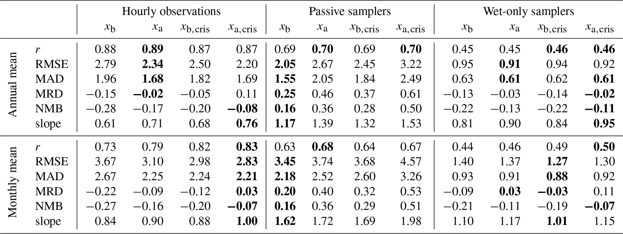
The modeled NH₃ surface concentration and ${\mathrm{NH}}_{\mathrm{4}}^{+}$ deposition fields were compared to in situ observations. The statistics are summarized in Table 2. Our results illustrate that the strength of the first method, i.e., CrIS-based NH₃ time factors, primarily lies in improving the temporal distribution of the NH₃ emissions. Compared to in situ networks, an overall increase in correlation coefficient and clear decrease in differences (RMSE, MAD, MRD, NMB) at the hourly observation and the wet-only sampler sites were observed. Moreover, time series of observed daily NH₃ surface concentrations illustrate that using the CrIS-based NH₃ time factors resulted in a better representation of both the onset and duration of the spring NH₃ peak in the Netherlands. The second method, data assimilation of the CrIS NH₃ columns with the LETKF, improved the comparability to in situ observation both spatially and temporally. Here, higher correlations with both annual and monthly observed mean NH₃ surface concentrations and ${\mathrm{NH}}_{\mathrm{4}}^{+}$ wet deposition were observed. This method also led to a decrease in differences (RMSE, MAD, MRD, NMB) at the hourly observation and the wet-only sampler sites. The mean NH₃ surface concentrations at the passive sampler sites, on the other hand, were more strongly overestimated in both methods. The comparison to in situ observations improved the most, both spatially and temporally, in the run where both methods are combined (x_a,CrIS). This illustrates that an initial, observation-based, rescaling of the NH₃ emissions enhances the adaptability of the LETKF, herewith thus improving the modeled NH₃ surface concentration and ${\mathrm{NH}}_{\mathrm{4}}^{+}$ wet deposition fields.

4.2 Discussion

4.2.1 CrIS-based NH₃ time factors

The temporal redistribution of the NH₃ emissions after using the fitted CrIS-based NH₃ time factors led to a significantly better representation of the temporal variation in NH₃ emissions, especially the spring peak. Compared to in situ observations, however, the NH₃ surface concentrations were overestimated in late summer and autumn (August to October). Further fine-tuning of the fitting algorithm could help to reduce the current overestimation and potentially improve the fitted NH₃ time factors. For example, data filtering and selection criteria could be adapted. Narrowing the selection radius used for selecting the CrIS NH₃ observations could for instance lead to a better representation of the NH₃ concentrations locally. This, however, may not always be possible, as a minimum number of observations is needed for a converging fit. Furthermore, the fitting algorithm currently does not allow for NH₃ area emissions during winter, because of the limited number of available CrIS observations at this time. As a result, the fitted NH₃ time factors show a relatively steep increase at the beginning of spring and a decrease at the beginning of winter. This could lead to step-like functions in areas where clear NH₃ peaks in the CrIS NH₃ data are absent. However, as this mainly occurs in areas with little to no NH₃ emissions, this should not severely impact the modeled NH₃ concentrations in this study.

4.2.2 Local ensemble transform Kalman filter

The NH₃ emission updates computed by the local ensemble transform Kalman filter (LETKF) always remain tied to the initial model fields by a certain uncertainty range. As such, data assimilation of the CrIS NH₃ columns with the LETKF is mainly suitable for fine-tuning NH₃ emissions in regions where the NH₃ emissions are already relatively well known. The chosen LETKF configuration is for instance not able to correct for missing NH₃ emissions in areas where few or no initial NH₃ emissions are present. Furthermore, the LETKF is unable to resolve temporal patterns well without sensible input, as was illustrated in an experiment with homogeneous NH₃ emission fields (Sect. S1).

The LETKF filter settings used in this modeling setup (ρ = 15 km, σ = 0.5, τ = 3 d) led to a maximum emission increase of roughly ∼ 30 % on the initial NH₃ emissions for long-term simulations. The choice of these filter settings affects the adaptability of the LETKF, i.e., the achievable emission adjustments by correction factors. In this study, a temporal length scale τ of 3 d was chosen as a compromise between short timescales needed for irregular emissions (e.g., fertilizer application) and longer timescales needed for regular emissions (e.g., stables and other point sources). Moreover, it matches the average satellite revisiting time per grid cell given the number of CrIS NH₃ observations left after data selection (Fig. S21). A spatial correlation of ρ = 15 km was chosen because it matches the footprint size of the satellite. Furthermore, as shown in Sect. S1, increasing standard deviation σ leads to larger, positive β factors. To prevent further overestimations in background regions, a σ of 0.5 was used for this region.

The current LETKF settings could for instance be improved by using spatially varying τ values. The choice of τ could be optimized for each emission category in the model. Locations with fertilizer application as a dominant NH₃ emission source could for instance be set to lower τ values than locations with predominantly regular NH₃ sources. Another way to optimize the filter settings would be to study time series of the model–satellite discrepancies in more detail and base the choice of τ on this. A more apparent memory effect (i.e., higher τ) would be useful in areas with consistent model–satellite discrepancies, whereas in areas with incidental differences a lower τ would be more appropriate. Similarly, statistical analysis of the already computed emission perturbation factors β could be performed. In this study, the model uncertainty follows a normal distribution in the current model setup. The distribution of the NH₃ concentrations, however, is, in reality, better approximated by a log-normal distribution. It would therefore be more realistic to use a log-normal distribution for the model uncertainty as well. This would incidentally allow for larger correction factors when high NH₃ peaks are observed, for instance after fertilizer application.

In the current LETKF model setup, only the NH₃ emissions are perturbed. Thus, the discrepancies between the observed and modeled NH₃ concentrations are currently fully assigned to errors in the underlying model NH₃ emissions. However, other model uncertainties could also cause these discrepancies, for instance uncertainties in other model inputs (e.g., other trace gas emissions) or parameterizations (e.g., deposition routines). In a follow-up study, it would be interesting to further investigate the effect of an inverted LETKF setup, where model sink terms are perturbed instead of the source terms. However, the current setup is the most obvious as the NH₃ emissions are likely the largest source of model uncertainty in this area. It would also be interesting to assimilate in situ observations and/or other satellite products (for instance IASI NH₃) simultaneously in a follow-up study.

4.2.3 Data products

Direct comparison of the observed and simulated NH₃ columns showed distinctly lower NH₃ total column concentrations in LOTOS-EUROS. This discrepancy could be the result of a systematic underestimation of the input NH₃ emission in LOTOS-EUROS or other model uncertainties. It could, on the other hand, also be partially related to the CrIS observations themselves. Here, only CrIS observations with the highest-quality flag (QF = 5) were used, which for instance could have resulted in a bias towards observations with higher NH₃ concentrations or during good weather (e.g., no clouds), as these observations usually have a lower uncertainty. Moreover, an offset of approximately ∼ 0.5 × 10¹⁶ molecules cm⁻² is observed. This seems to be the effect of the detection limit of the CrIS instrument, which is unable to detect very low NH₃ concentrations. Furthermore, this, too, could be enhanced by the relatively strict data selection criteria used in this study, which favors higher NH₃ concentrations that usually have a lower uncertainty. In the next version of the CrIS NH₃ product, which was not yet available for this study, these non-detects are addressed. This might lead to lower NH₃ concentrations in background regions and partially solve this discrepancy. Moreover, this could also result in a better comparison with observations of the passive sampler networks.

The differences between the modeled and observed NH₃ concentrations and ${\mathrm{NH}}_{\mathrm{4}}^{+}$ wet deposition fields are partially related to limitations in the spatial representativeness of the in situ observations. The comparison of the different model runs to in situ observations showed an overall overestimation at the passive sampler sites. These sites are mainly located in nature areas and therefore assumed to be representative of background regions with little to no NH₃ emissions. However, especially in the Netherlands, the landscape layout is very heterogenous, and the nature areas are relatively small. As a result, at the current model grid size, each model pixel is likely to include other landscape elements than nature alone. The larger model scale averages out the small-scale effects, thus leading to an overestimation. The opposite is true for the hourly observation sites located in medium to high NH₃ emission regimes. Especially at sites close to NH₃ emission sources, an underestimation is expected.

4.2.4 Conclusions

To conclude, satellite-observed CrIS NH₃ time series are helpful in improving NH₃ emissions, both spatially and temporally. Our results illustrated that CrIS NH₃ surface concentrations can be successfully used to fit spatially variable NH₃ time factors, which allows us to improve temporal NH₃ emission distributions relatively easily in a forward modeling setup. Comparison with in situ NH₃ surface concentrations and ${\mathrm{NH}}_{\mathrm{4}}^{+}$ wet deposition observations showed that the fitted CrIS-based NH₃ time factors were particularly useful for adjusting the timing and duration of the NH₃ spring peak in medium to high NH₃ regimes. Moreover, the comparison showed that the CrIS-based NH₃ time factors improve the temporal distribution of the modeled NH₃ surface concentrations and ${\mathrm{NH}}_{\mathrm{4}}^{+}$ wet deposition fields. Our results show that data assimilation of the CrIS NH₃ columns data with the local ensemble transform Kalman filter (LETKF) improves the comparability with in situ observations both spatially and, to a lesser extent, temporally, too. As the adaptability of the LETKF is limited by the uncertainty in the modeled fields, the strength of this method primarily lies in fine-tuning pre-existing NH₃ emission patterns. As a result, this method proved particularly useful for improving spatial NH₃ distributions in long-term simulations. Moreover, our results illustrated that combining both methods enhanced the adaptability of the LETKF and led to the largest improvements in modeled NH₃ surface concentration and ${\mathrm{NH}}_{\mathrm{4}}^{+}$ wet deposition fields compared to in situ observations.