Eddy covariance measurements highlight sources of nitrogen oxide emissions missing from inventories for central London

During March–June 2017 emissions of nitrogen oxides were measured via eddy covariance at the British Telecom Tower in central London, UK. Through the use of a footprint model the expected emissions were simulated from the spatially resolved National Atmospheric Emissions Inventory for 2017 and compared with the measured emissions. These simulated emissions were shown to underestimate measured emissions during the daytime by a factor of 1.48, but they agreed well overnight. Furthermore, underestimations were spatially mapped, and the areas around the measurement site responsible for differences in measured and simulated emissions were inferred. It was observed that areas of higher traffic, such as major roads near national rail stations, showed the greatest underestimation by the simulated emissions. These discrepancies are partially attributed to a combination of the inventory not fully capturing traffic conditions in central London and both the spatial and temporal resolution of the inventory not fully describing the high heterogeneity of the urban centre. Understanding of this underestimation may be further improved with longer measurement time series to better understand temporal variation and improved temporal scaling factors to better simulate sub-annual emissions.

1 Introduction

Nitrogen oxides (NO_x), the sum of nitrogen oxide (NO) and nitrogen dioxide (NO₂), are air pollutants which in the urban environment are mainly emitted from anthropogenic combustion processes as NO and oxidised in the atmosphere, forming NO₂. NO₂ has been shown to exacerbate pre-existing respiratory and cardiovascular conditions (Forastiere et al., 2005). Furthermore, NO_x is responsible for the formation of ground-level ozone (O₃) in the presence of peroxy radicals (from the oxidation of volatile organic compounds) and is involved in the formation of nitrate aerosols. Tropospheric O₃ has been shown to cause pulmonary conditions and has been linked to the development of asthma (McConnell et al., 2002; Saldiva et al., 2005).

London regularly faces issues with NO₂ concentrations, often breaching various air quality limits. NO_x concentrations are measured at a combination of sites from the Automatic Rural and Urban Network (AURN) and the London Air Quality Network (LAQN) across the Greater London area. Average annual concentrations for the 101 sites are shown in Fig. 1, 57 of which breached the European annual mean air quality limit of 40 µg m⁻³ in 2017 (Council of European Union, 2008). Sites classified as kerbside or roadside make up 51 of these, linking a lot of London's NO₂ issues to the transport sector.

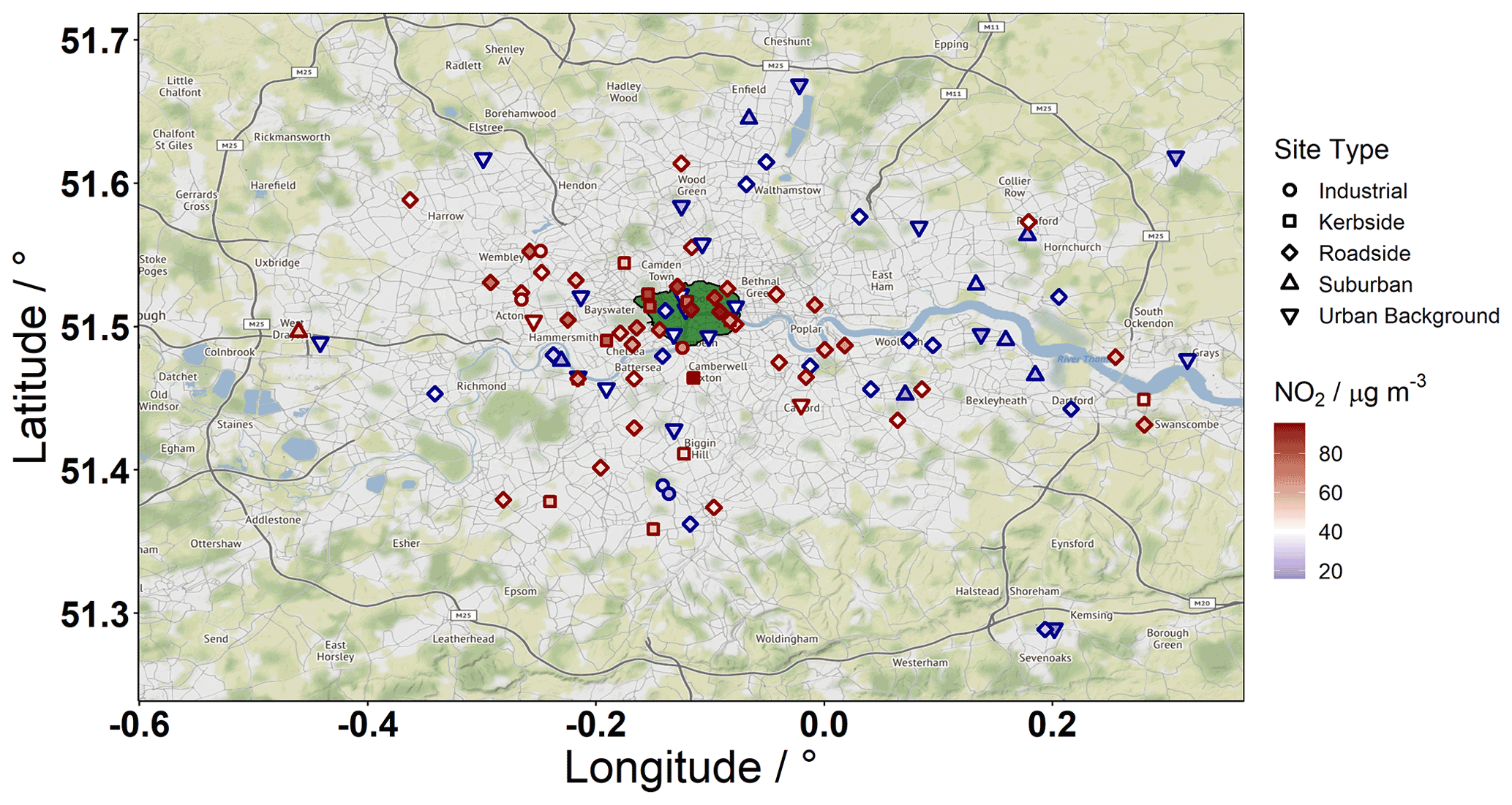
Figure 1 101 air quality monitoring sites located in and around Greater London. Sites are coloured by their annual mean NO₂ concentration for 2017 (µg m⁻³). Point shape denotes the type of measurement site. Point borders change from blue to red above the 40 µg m⁻³ air quality limit. 57 sites had annual mean concentrations above this limit in 2017. The area which encompasses the congestion charging zone and ultra-low emissions zone is shown in green. Map tiles by Stamen Design, under CC BY 3.0. Data © OpenStreetMap contributors 2021. Distributed under the Open Data Commons Open Database License (ODbL) v1.0. Tiles accessed via the ggmap R package (Kahle and Wickham, 2013).

According to the National Atmospheric Emissions Inventory (NAEI), road transport a well as domestic and industrial combustion are the key sources of NO_x in Greater London. Road transport is the largest single contributing sector, with diesel engines receiving much of the attention and blame for the high concentrations seen in the London. Road transport has been the target of policy intervention in the city such as the congestion charging zone (CCZ) introduced in 2003, which imposed a daily charge for vehicles driving into the centre of London from Monday to Friday between 07:00 and 18:00. This policy was not intended to improve air quality but rather reduce congestion and CO₂ emissions. Very little change was seen in NO_x concentrations, and at places such as Marylebone Road, a major thoroughfare which forms the northern border of the CCZ, increases in ambient NO₂ were recorded after adjusting for meteorology (Transport for London, 2016; Grange and Carslaw, 2019). Grange and Carslaw (2019) also showed that the CCZ increased effective concentrations of NO₂ at Marylebone Road and they did not approach pre-CCZ levels until 2011, with the improvement of buses from Euro III to Euro V emissions standards (5 to 2 g kWh⁻¹ of NO_x) on routes on and around Marylebone Road. Further decline was noted with the introduction of Euro VI and hybrid buses up to 2016, when the study ended. This illustrates the difficulty in predicting the effect of policy interventions on air quality and the importance of considering the effect of polices that do not explicitly target air quality but nevertheless may have indirect consequences. Accurate emissions inventories can help with this task, as they are often the primary input to air quality models.

London's low emission zone (LEZ), introduced in 2009, aimed to improve air quality by reducing the pollution from heavy vehicles either by reducing their number or encouraging improved emissions control technology. This was shown to have reduced ambient NO₂ levels and the number of people exposed to exceedances of the 40 µg m⁻³ annual air quality limit in several boroughs (Mudway et al., 2019).

In April 2019 London introduced the ultra-low emissions zone (ULEZ) specifically targeting vehicle emissions. The charge applies at all times to vehicles that do not meet specific Euro classes for their vehicle type (motorbikes Euro 3, petrol cars Euro 4, diesel cars and larger vehicles Euro 6; 0.15, 0.08, and 0.08 g km⁻¹ of NO_x, respectively) and is expected to have had a greater impact on NO_x emissions in London (Greater London Authority, 2021).

Whilst there are large numbers of ambient concentration measurements available, limited emissions measurements have been made in London. The NAEI provides UK-wide emissions estimates, and for Greater London they declined from 120 to 45 kt yr⁻¹ (62 %) between 1998 and 2017. NO_x concentrations were reduced by 28 %, 40 %, and 45 % on average at roadside, kerbside, and urban background sites, respectively (Fig. 2).

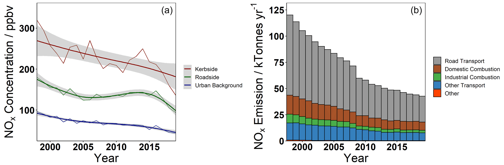
Figure 2 (a) Change in average concentration at roadside, kerbside, and background sites in Greater London between 1998 and 2019. All sites with available data were first annually averaged, followed by calculating the grand mean of all sites of a given type per year. A generalised additive model (GAM) was fit to the data to produce the smooth line, and shading shows the standard error in this fit. (b) NAEI emissions for Greater London. As historical spatially resolved versions of the NAEI are not available, these data were generated by scaling each sector of the spatially resolved inventory for 2019 within the Greater London area by their relative value in the historical UK total emissions data. This assumes that London has generally followed the UK trend in NO_x emissions.

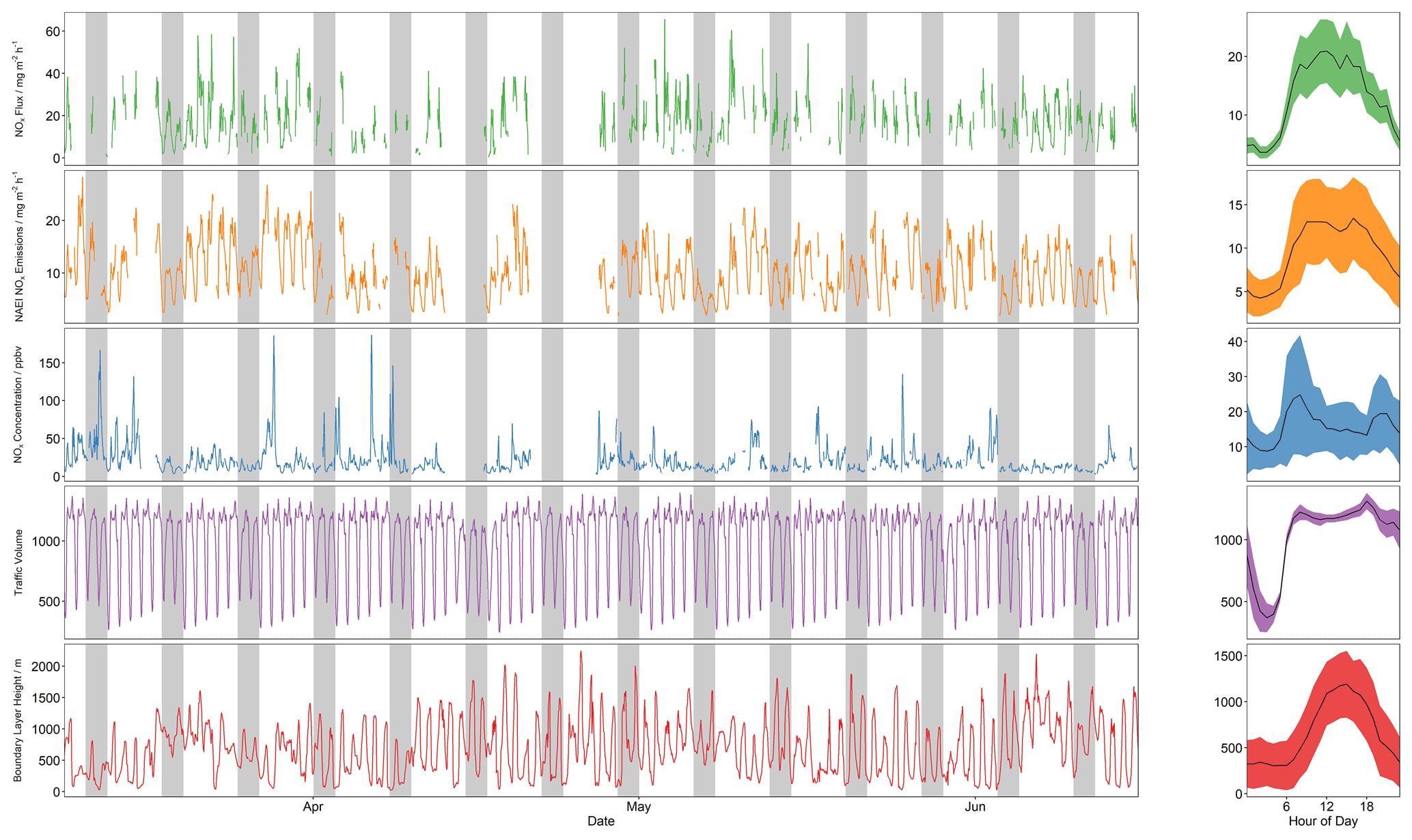
Figure 3 Time series (left) and median diurnal profiles (right) of (top to bottom) measured of NO_x flux, simulated emissions from the NAEI, NO_x concentration, traffic volume, and modelled boundary layer height. Shaded periods on time series highlight weekends. Shaded regions on diurnal profiles refer to median absolute deviation in diurnal averaging, except in the case of NO_x flux; this region represents the average total error in flux measurement.

Eddy covariance (EC) measurements of NO and NO₂ fluxes were previously made at the British Telecom (BT) Tower during the Clean Air for London (ClearfLo) project's intensive observation periods in 2012–2013 and from an aircraft during the Ozone Precursor Fluxes in an Urban Environment (OPFUE) campaign in 2014 (Lee et al., 2015; Vaughan et al., 2016). During ClearfLo Lee et al. (2015) collected EC data at the BT Tower for 36 d in June–August 2012 and 28 d in March–April 2013. These measurements suggested that the NAEI underestimated the NO_x emission by a factor of 1.36–2.2 and was largest for fluxes measured to the east of the tower, across all footprint distances. Diurnal profiles of NO_x correlated closely with diurnal profiles of traffic flow surrounding the tower.

Airborne EC NO_x fluxes were collected during three flights in July 2013. Vaughan et al. (2016) used these data to provide insight into the spatial change in emissions across Greater London and found the underestimation of NO_x emission by the NAEI, in central London, to be similar to that found by Lee et al. (2015). The agreement between the measurement and inventory improved significantly outside central London. Both of these studies also compared their results to the London Atmospheric Emissions Inventory (LAEI), an inventory which focuses on the Greater London area, and an enhancement of the LAEI using on-road emissions data collected via remote sensing. Both of these comparisons further improved agreement and suggested that the traffic sector is responsible for much of the disagreement. The discrepancies between NO_x emission measurements and inventories correlate with fleet composition in central London, where taxis and buses outnumber private vehicles (Vaughan, 2017).

We report on EC emissions measurements of NO_x from the BT Tower collected during the spring and summer of 2017. The resulting time series is compared to the NAEI and LAEI, and it supports the finding of previous studies that these inventories underestimate measured values. Additionally, these data are further developed into spatially resolved maps with the aid of footprint modelling, and we estimated the spatial distribution of these hitherto under-reported NO_x sources. In this article we will discuss the eddy covariance experimental setup, including the site, instrumentation, and data processing (Sect. 2.1–2.2). We also cover in detail several sources of uncertainty in the experimental setup and provide a discussion on these with respect to the interpretation of results (Sect. 2.2.1). In Sect. 2.3 we cover the emissions inventories explored in this study and the footprint modelling used to simulate an emissions time series from them. The resulting measurements are discussed in Sect. 3.1, and their comparison with simulated emissions time series is presented in Sect. 3.2.

2 Methodology

2.1 Site description and instrumentation

Measurements of NO and NO₂ mixing ratios were made at the BT Tower between March and June 2017 using a closed-path dual-channel Air Quality Design (AQD) chemiluminescence analyser equipped with a blue-light converter for NO₂. The instrument is similar to those described by Lee et al. (2009) and Squires et al. (2020) and provided a sampling rate of 5 Hz. The site is a 177 m tall tower located in central London in the borough of Camden, south of Euston Road and north-east of Hyde Park (latitude and longitude: 51.521, −0.139^∘). The surroundings are typical of the central London area with a mixture of larger arterial roads, high traffic density, and smaller side streets interconnecting them. Traffic is slow-moving, and stop–start driving conditions are common during busier periods. Surrounding buildings within a 3 km radius average ∼ 50 m tall, with the next tallest building measuring ∼ 130 m, placing the sampling height above the urban canopy (Environment Agency, 2017).

A 3D ultrasonic anemometer (Gill R3-50) was mounted on a mast atop the tower, co-located with the gas analyser sample line inlet, providing a measurement height of 190 m. The anemometer provided 3D wind vectors and temperature derived from the speed of sound. Air was pumped down the ∼ 45 m sample line (PFA OD $\mathrm{3}/{\mathrm{8}}^{\prime \prime }$) with a target flow rate of 25 L min⁻¹ to the instrument, which was located on the 35th floor. During March–June 2017 the prevailing wind direction was between west and south-westerly, and the median wind speed was ∼ 6.7 m s⁻¹.

2.1.1 Instrument calibration

NO and NO_x channel sensitivities and NO₂ conversion efficiency were calibrated automatically every 63 h such that data loss from calibrations was spread over the diurnal cycle. A 5.2 ppmv NO standard, traceable to the National Physical Laboratory (NPL) scale, was used as a span gas and injected at 10 sccm into the sample flow. Coefficients were linearly interpolated to 1 min resolution before being applied to the data. Both channels were zeroed for 2 min hourly using a combination of scrubbed ambient air (generated from an external Sofnofil and activated charcoal trap) and a pre-chamber zero (O₃ is introduced early such that chemiluminescence occurs away from the detector). Conversion efficiency was determined via gas-phase titration of the calibration gas with O₃ generated from an internal mercury lamp. NO and NO_x channel sensitivities were (2.4 ± 0.3) and (3.8 ± 0.6) counts pptv⁻¹, respectively, and conversion efficiency was (70 ± 3) % over the measurement period.

2.2 Eddy covariance calculations

Eddy covariance calculations were performed using the eddy4R (Metzger et al., 2017) family of R software packages and followed the general procedure in Fig. A1. Calibrations were first applied as described above, and the mixing ratio and wind vector data streams were joined into hourly data files. Mixing ratios were converted to mole fractions for analysis, and the calculations assumed that this was dry mole fraction. In reality this was not the case due to a lack of water vapour measurements within the AQD instrument. While closed-path analysers are affected by density fluctuations from changes in temperature to a lesser extent than open-path ones, humidity can still have an effect. This effect is proportional to the concentration flux ratio (Pattey et al., 1992) and was determined to be much less than 1 % for these measurements, in line with other NO_x measurements made in a similar experimental setup (Squires et al., 2020). Fluxes were calculated for NO and NO₂ individually and converted to mass units using their respective molecular weights before combination into NO_x fluxes. Fluxes were aggregated over hourly periods, and those with less than 90 % data coverage for each period were discarded. Hourly periods were used over the more traditional half-hourly EC aggregation period due to the height of the measurement tower. At 190 m, lower-frequency turbulence will have a greater contribution to the flux, so a longer aggregation reduces losses from these. Additionally, scaling factors for the emissions inventories were only available to hourly resolution, so there would be no analytical gain from a higher-resolution time series. The hourly aggregation period was tested for its appropriateness for these data by comparing it with fluxes calculated with a half-hourly aggregation period and subsequently averaging to 1 h, with no significant difference between the aggregation periods being found. Spikes were removed from the data using the median filter approach described by Brock (1986) and Starkenburg et al. (2016). Subsequently, the lag between the sonic anemometer and the AQD instrument measurements (introduced by the spatial separation of the receptors) was corrected using high-pass-filtered maximisation of the cross-correlation maximisation (Hartmann et al., 2018). Considering the sample line dimensions and flow rate, hourly determined lags were accepted in the range of 0 and −10 s; if a calculated lag fell outside this range, the median of −6.6 s (for NO) and −6.4 s (for NO₂) was used. Double coordinate rotation was performed to align the v wind vector with the mean flow and reduce the average vertical wind to zero. The fluctuating components were calculated as the deviation from a linear trend calculated per hour. After the calculation of covariances, stationarity tests after Foken and Wichura (1996) were performed, and random and systematic errors were calculated after Mann and Lenschow (1994). Errors presented in this paper are the quadratic combination of these two errors. Data were finally flagged using eddy4R's quality control scheme, which produces a quality flag based upon a combination of input data validation, stationarity, and integrated turbulence characteristics (Smith and Metzger, 2013). This resulted in 1556 h of high-quality fluxes (66 % coverage) for the measurement period.

2.2.1 Additional uncertainties

Vertical flux divergence

EC provides measurements of local flux at the receptor. These are related, but not identical, to the surface flux. This surface flux is what is comparable to the emissions inventories. The local flux can diverge from the surface flux due to the vertical separation. Turbulence properties are not vertically uniform through the boundary layer; as the top of the boundary layer is approached (the entrainment zone) vertical turbulent transport is reduced, turbulence properties are more disconnected from the surface, and the applicability of EC is diminished. This results in a vertical gradient of the turbulent flux: vertical flux divergence. This also results in concentration enhancements below the measurement height, causing a gradient throughout the boundary layer, and is described as storage flux. The flux not registered by the receptor can be estimated from either of these perspectives: from the rate of change in concentration with height (i.e. storage) or from proportionality with the entrainment height (i.e. vertical flux divergence). In the case of measurements made at 190 m above the surface, the measurement height is an appreciable proportion of the boundary layer height depending on the time of day and meteorological conditions. To account for this we apply a correction that assumes linear divergence of the vertical flux as a function of effective measurement height and effective entrainment height (Eq. 1) (Deardorff, 1974; Sorbjan, 2006; Metzger et al., 2012):

$$\begin{array}{}\text{(1)}& F^{\prime }={\displaystyle \frac{F}{\mathrm{1}-\frac{z_{\mathrm{m}}-z_{\mathrm{c}}}{z_i}}},\end{array}$$

where

• F is the flux prior to correction,

• F^′ is the flux following correction,

• z_m is the measurement height of 190 m,

• z_c is the height of the constant flux layer, defined as 10 % of the boundary layer height (Foken, 2017), and

• z_i is the entrainment height, defined as 80 % of the boundary layer height.

We apply this correction only when z_m>z_c, as in the reverse case the sensor location can be considered in the constant flux layer and should not require correction.

Modelled boundary layer height data from the ECMWF ReAnalysis 5 0.25×0.25^∘ global meteorology product (ERA5) were used in the determination of the correction factor (Copernicus Climate Change Service Climate Data Store (CDS), 2017). Modelled boundary layer height was also obtained for the period 6 January to 9 February 2012 for which the measured boundary layer height is available for central London from the ClearfLo campaign (Bohnenstengel et al., 2015). These data had a Pearson correlation of 0.59, and an orthogonal regression of modelled vs. measured gave a slope of 0.52 and an intercept of 245 m. Due to the correction's sensitivity to the boundary layer height, this offset changes the average diurnal profile by between 1.8 % and 82 %. If we correct the boundary layer height for 2017 by the offset and slope calculated for the 2012 data, this change is reduced to between 0 % and 27 %. The inclusion of the constant flux layer term in the equation also has a substantial impact on the magnitude of this correction. The correction in the case using the corrected boundary layer height without the constant flux layer term is in the range of 10 % and 52 %. The effect of all of these corrections is shown in Fig. A2.

The divergence has been assessed via this method due to the lack of gradient measurements available at the tower, and the single point correction as used by Squires et al. (2020) was not applied, as there was no appreciable difference between the corrected and uncorrected fluxes. This is more likely due to attenuation of the concentration enrichments at this measurement height rather than the lack of stored flux. In the absence of a vertical profile, the single measurement at the top of the air column would provide a more uncertain estimate of the change in concentration between the surface and the EC sensor height than a correction derived from a single measurement halfway between the surface and the EC sensor height. The higher the EC sensor, the more poorly constrained this approach would become. Therefore, we apply the top-down flux divergence approach, as its use of boundary layer height provides a more constrained method of estimating this loss.

We do not apply this correction to the data presented in this study due to the uncertainty in the boundary layer height, but in the best case of these calculations (corrected boundary layer height and constant flux layer term), the largest absolute change to the diurnal profile is 2.23 mg m⁻² h⁻¹. We suggest future experiments at this site consider the determination of this storage term in more detail.

Night-time stationarity

When flagging data for quality control, the stationarity criterion is more readily violated when the magnitude of the calculated flux is lower. Stationarity is considered violated if the flux calculated for a subsection of the aggregation period deviates from the flux calculated for the whole aggregation period by a predefined fraction (∼ 30 %) (Foken and Wichura, 1996). For this reason it is more likely for the flux calculated for a subsection of an aggregation period to deviate from the whole the smaller the total flux for that period is, skewing the data set towards larger fluxes.

In Fig. 4a this is shown to be the case, with the percentage of records flagged by the quality control routine rising sharply once the magnitude of the flux falls below 10 mg m⁻² h⁻¹. Furthermore, as NO_x emissions followed a strong diurnal profile, the lower night-time values are flagged more regularly, as seen in Fig. 4b. By removing these flagged data, there is risk that the resulting values are biased high, especially at night, when stable atmospheric stratification is more likely to occur.

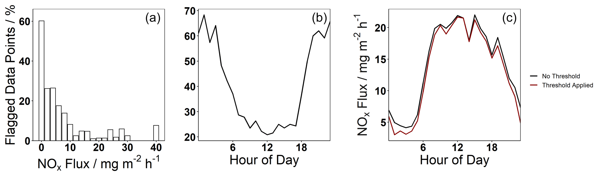
Figure 4 (a) Percentage of flux records flagged by quality control routines in 2 mg m⁻² h⁻¹ bins. (b) Percentage of flux records flagged by quality control routines by hour of day. (c) NO_x flux diurnal cycle; black has had all records flagged by quality control routines removed, and red has only had them removed if the flux magnitude was also greater than 5 mg m⁻² h⁻¹.

To quantify the effect of removing the values, the diurnal profile for NO_x flux was calculated twice in Fig. 4c. The black trace removes all data that have been flagged by the quality control routines, and the red has only removed flagged points at which the magnitude of the flux exceeded a 5 mg m⁻² h⁻¹ threshold. A slight high bias was observed when the stationarity criterion was not limited by flux magnitude, and this bias was greatest at night up to ∼ 20 %. For this analysis, all data points flagged for non-stationarity have been removed, but this bias should be considered during interpretation.

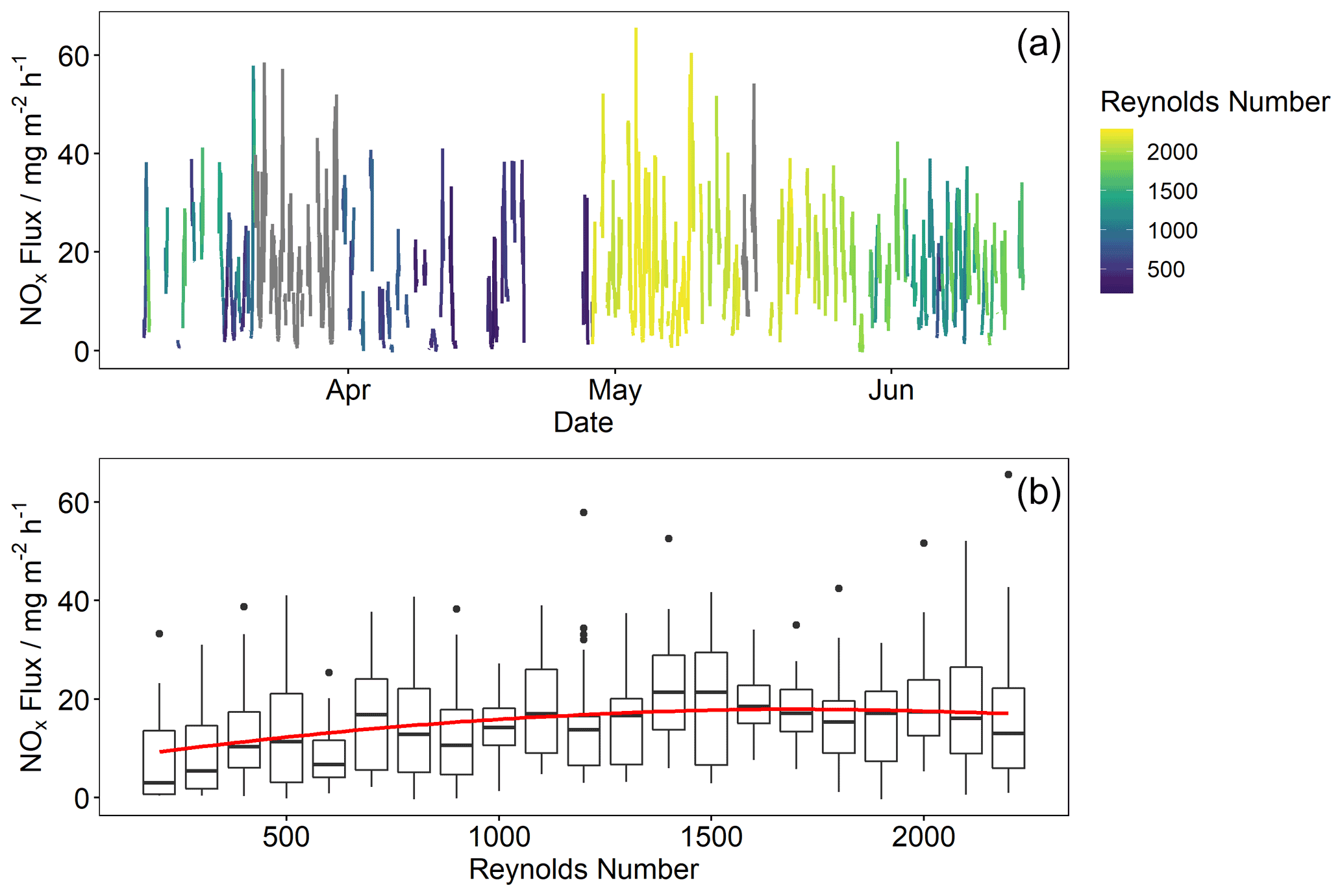
Figure 5 (a) Unfiltered NO_x flux coloured by Reynolds number. Grey periods are when sample flow data are unavailable. (b) NO_x flux against binned Reynolds number (bin width 100). Boxes show the median value as the horizontal bar as well as the 25th and 75th percentile at the limits of the box. Whiskers extend to 1.5 times the interquartile range, and data that fall outside this range are plotted as points. A loess-smoothed fit shows increasing dependency of NO_x flux on Reynolds numbers below 1500.

Sample line turbulence and high-frequency corrections

Turbulent flow through the sampling line is a prerequisite for EC measurements. Laminar flow in the sample line causes the gas which interacts with the tubing wall to flow slower than that in the centre of the line, meaning that air parcels contain asynchronous samples, primarily causing high-frequency losses (Aubinet et al., 2012; Leuning and King, 1992). The Reynolds number (Re) is a quantity which is used to quantify turbulent flow of a fluid. While the transition is not well defined, Aubinet et al. (2012) suggest a Re value of <2100 to be laminar and >3000 to be turbulent. More generally, smaller values of Re produce laminar flow, and larger values produce turbulent flow. During the measurements at the BT Tower, flow rates in the sample line varied between 26.7 and 2.8 L min⁻¹ due to the line's particle filter becoming blocked. The filter was only irregularly replaced as access to the inlet location was limited. The Reynolds number was calculated as in Eq. (2) and ranged between 120 and 2300. This leads to periods of time when the sample line was under a transitional or laminar regime:

$$\begin{array}{}\text{(2)}& Re={\displaystyle \frac{\mathit{\rho }\mathit{\upsilon }d}{\mathit{\mu }}},\end{array}$$

where

• Re is the Reynolds number,

• ρ is the density of air calculated at the sample line pressure and temperature (kg m⁻³),

• υ is the transit speed of the air down the sample line (m s⁻¹),

• d is the internal diameter of the sample line of 0.00638 m, and

• μ is the absolute viscosity of air, calculated here as the Sutherland viscosity (Sutherland, 1893).

In Fig. 5 the relationship of the Reynolds number with raw NO and NO_x fluxes is presented. The fitting of the loess-smoothed line on the binned data reveals a dependence of flux on Reynolds numbers below 1500. However, while there is this trend, there is still variability in the data during these times, so no correction has been applied, but it should be borne in mind that measured fluxes are underestimates due to this loss. The flux loss due to lack of turbulence in the sample line will primarily relate to the high-frequency component of the measurement, and some quantification of these is discussed below.

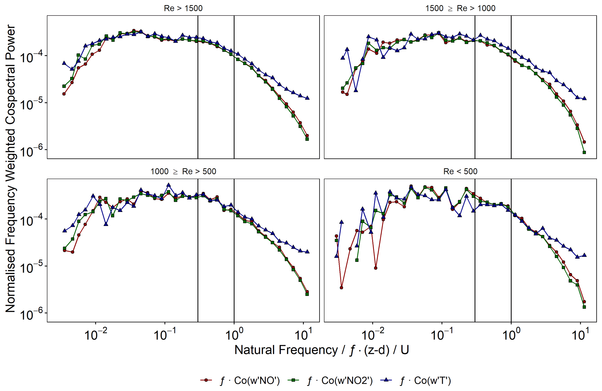
Figure 6 Normalised co-spectra of vertical wind with NO (red, circle), NO₂ (green, square), and temperature (dark blue, triangle). Co-spectra are grouped by main sample line Reynolds number. Vertical bars mark 0.3 and 1 Hz; data at frequencies greater than these have been used to derive the correction factors presented in Table 1.

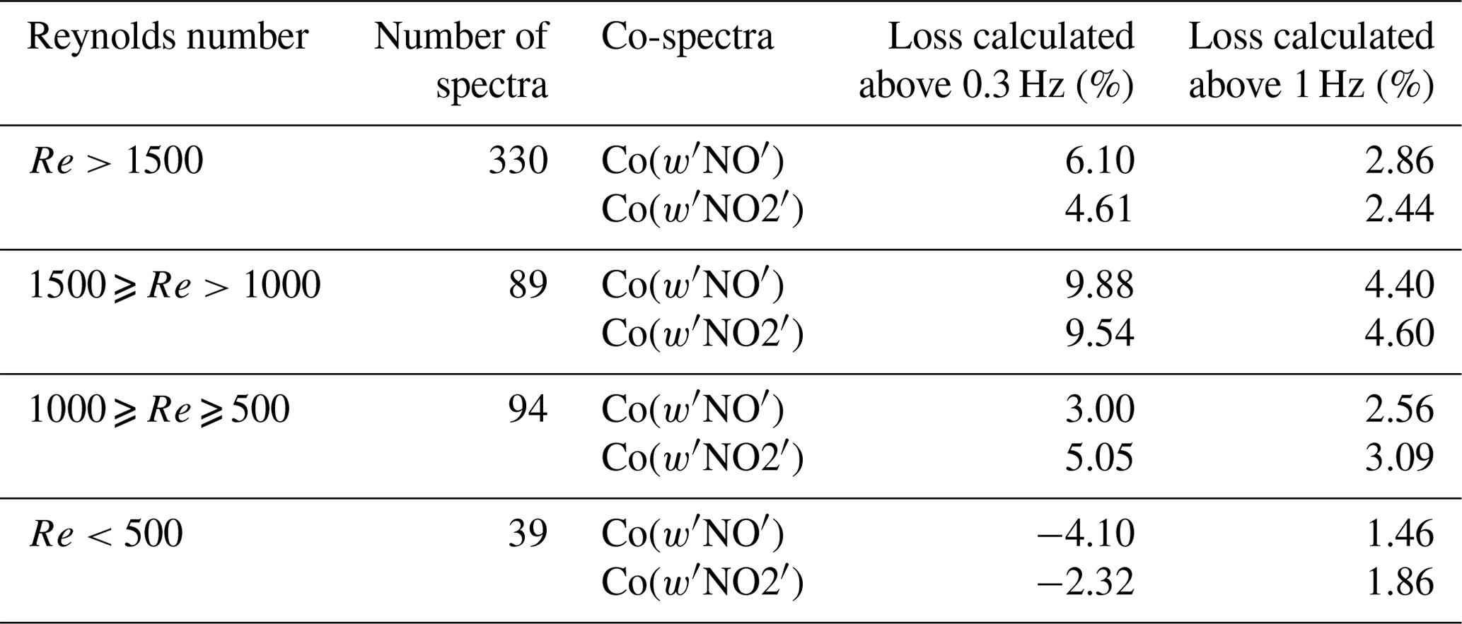
Due to its height the high-frequency contributions to fluxes measured at the BT Tower are expected to be small, with Helfter et al. (2016) noting that >70 % of the flux can be captured using an instrument running at 1 Hz. It was therefore expected that 5 Hz measurements would capture significantly more. To quantify this co-spectra were calculated for four different sample line regimes, as summarised in Table 1. These co-spectra were generated during periods when sensible heat flux was >50 W m⁻² and u^* was > 0.2 m s⁻¹ and divided into the Re groups. Each co-spectrum was normalised by the sum of its co-spectral power between 10⁻² and 10⁻¹ Hz to avoid low-frequency noise and preserve high-frequency loss. Co-spectra in each Re group were averaged (median) into logarithmically equally spaced frequency bins. Figure 6 shows the resulting spectra across the groups. Co(w^′NO^′) and Co(w^′NO2^′) deviate from Co($w^{\prime }{T}^{\prime }$) towards the high-frequency end of each spectrum, which is likely due to sample line attenuation as all three scalar quantities were captured at 5 Hz. The percentage loss in each case was calculated from data above 0.3 and 1 Hz. This was due to noise in the Re<500 spectra, suggesting that a negative correction was required. This noise likely arises from the limited number of spectra in the regime that could be averaged. However, the remaining three groups did not show a trend in high-frequency loss with Re, with values between 5 % and 10 % when the loss was calculated above 0.3 Hz. As the correction factors calculated are relatively small, they have not been applied here.

Table 1 High-frequency corrections derived for four sample line regimes using 0.3 and 1 Hz for the thresholds above which the correction was calculated.

2.3 Emissions inventories and footprint modelling

2.3.1 National Atmospheric Emissions Inventory

The NAEI is an annual emissions estimate for a variety of species in the UK from 1970 to present. Commissioned by the Department for Environment, Food and Rural Affairs, it is currently produced by Ricardo Energy & Environment and used to report to European Union and United Nations greenhouse gas and air pollutant monitoring programmes (Defra and BEIS, 2017; Council of European Union, 2016). Primarily, the inventory provides the total emissions estimates required by these monitoring programmes. Calculations assimilate activity data and emissions factors from a wide range of sources and combine them to form an emission. Emissions are categorised into the 11 source sectors defined by the Selected Nomenclature for sources of Air Pollutants (SNAP) along with point sources (Table A1) (European Environment Agency, 2016).

Once emissions estimates as a whole are compiled, the emissions are gridded using spatial information relevant to the SNAP sector. For example, road transport uses road network location, local fleet composition from automatic licence plate recognition statistics, and the annual average daily flow of traffic (Tsagatakis et al., 2018). Combined with emissions factor and activity data this provides a 1 km² resolution map of emissions in the UK. The 2017 version of the inventory is used in this work.

2.3.2 London Atmospheric Emissions Inventory

The LAEI is an annual emissions estimate that has been produced periodically since 2006 covering Greater London at a 1 km² resolution and also covering a wide range of air pollutants. It is commissioned and published by Transport for London and the Greater London Authority, with the most recent version built for 2016 (the version used in this work).

Four source sectors are included in the LAEI – transport, industrial and commercial, domestic, and miscellaneous. A notable difference here is the grouping of commercial sources with industrial, whereas in the NAEI they are grouped with domestic sources. The inventory used in this work was provided with hour of day scaling for the transport sector but has otherwise been treated the same as the NAEI.

2.3.3 Footprint modelling and simulated emissions estimates from inventories

To link the measured fluxes to the surface, we used the 2D footprint model by Kljun et al. (2004) with an additional cross-wind component by Metzger et al. (2012). This produced a footprint at 100 m × 100 m resolution per hour of flux data using meteorology statistics from the eddy covariance calculations, supplemented with modelled boundary layer height data from ERA5 (Copernicus Climate Change Service Climate Data Store (CDS), 2017) (boundary layer height is not a strong predictor in the footprint model, so the issues highlighted in section entitled “Sample line turbulence and high-frequency corrections” are not of concern here) and a surface roughness length of 1.1 m (the average within 5 km of the BT Tower, Drew et al., 2013). The footprint consists of a grid of these 100×100 m cells, each with an associated weighting of that area's contribution to the measured flux, for which the sum of the weights equals 1. The footprints were trimmed to 90 % of the total footprint weights; i.e. cells containing weights in the 10th percentile and below are removed, as above this threshold the footprint area grows rapidly, and the individual contribution from each grid cell is diminished. The average footprint for the measurement period can be found in Fig. 7 overlaid on a map of the four main sectors which contribute to the NAEI within the footprint area.

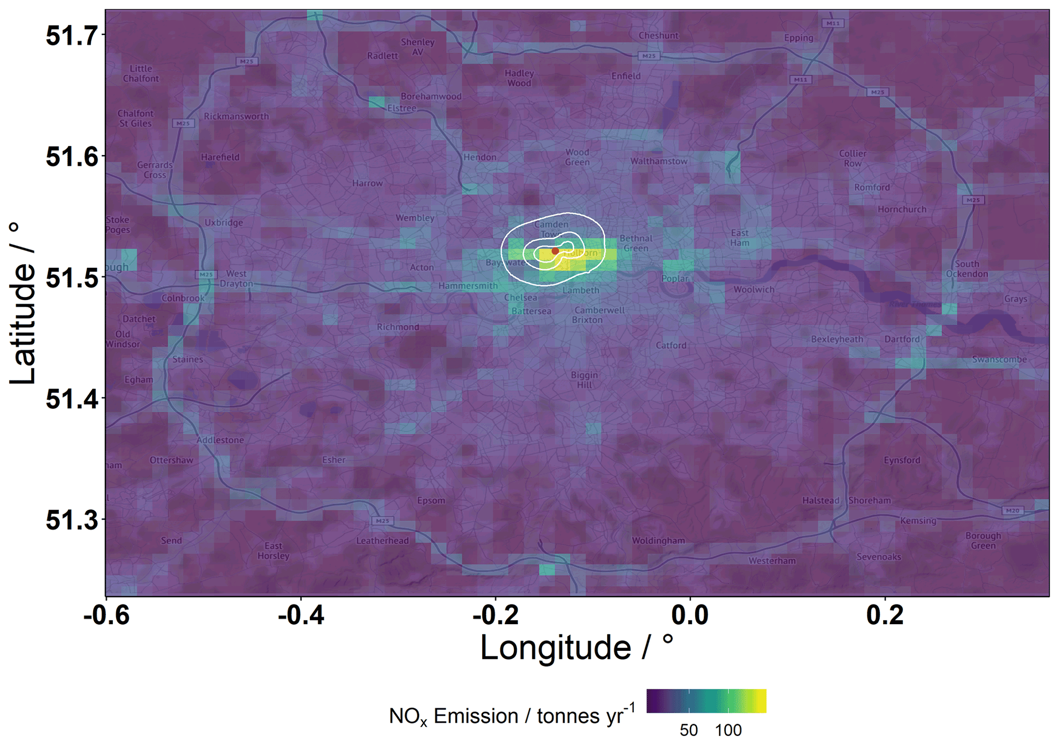
Figure 7 The sum of the NAEI layers corresponding to SNAP sectors 07, 02, 03, and 08 (see Table A1) to show the spatial distribution of the majority of NO_x emissions in central London. The 30 %, 60 %, and 90 % contributions to the flux footprint climatology for EC measurements made between March and July 2017 are shown in white. The red point shows the location of the BT Tower. Map tiles by Stamen Design, under CC BY 3.0. Data © OpenStreetMap contributors 2021. Distributed under the Open Data Commons Open Database License (ODbL) v1.0. Tiles accessed via the ggmap R package (Kahle and Wickham, 2013).

These hourly footprints were used to simulate an emissions time series from the spatially resolved NAEI for 2017 and LAEI for 2016. This was achieved by first extracting, on a by-sector basis, the inventory's grid cell (1 km²) values at the centre of each hourly footprint's (0.1 km²) grid cells. Each of these extracted values is weighted by that cell's contribution to the total hourly footprint and finally summing over all grid cells within the footprint. Each sector is then scaled to the month of year, day of week, and hour of day through the use of a selection of anthropogenic emissions profiles (Figs. A3 and A4) (Coleman et al., 2001; van der Gon et al., 2011; Brookes et al., 2013). These scaled sectors can then be summed to produce a total simulated emission as would be observed at the BT Tower. The same method was applied to all sectors within the LAEI except transport, which was provided with hourly scaling already applied, so this sector only used the day of week and month of year factors presented here.

The footprints were also used to map the measured and expected emissions spatially. This was achieved using the polarPlot() function from the openair R package (Carslaw and Ropkins, 2012). This function traditionally bins a scalar (often pollutant concentration) by wind speed and direction and produces an interpolated surface via GAM smoothing (Wood, 2017). Along-wind distance to the footprint maxima was provided to the function in place of wind speed, resulting in the output's radial axis having the units of metres. This could then be overlaid on a map. The along-wind distance to the footprint maxima is a simple method to produce these surface maps and neglects much of the information gained by the use of a 2D footprint model but allows for broad, qualitative interpretation of the data. More sophisticated methods of producing footprint topographies (Mauder et al., 2008; Kohnert et al., 2017) allow for a more direct quantitative approach but are out of scope of this study.

3 Results and discussion

3.1 Measurements

In Fig. 3, the time series of NO_x concentration and flux are shown, along with average traffic volume from a selection of automatic traffic counters within the footprint of the tower (Transport for London, 2018) and modelled boundary layer height from the ERA5 (Copernicus Climate Change Service Climate Data Store (CDS), 2017). Median NO_x concentrations showed two peaks at 08:00 (24.81 ppbv) and 21:00 (19.5 ppbv) (all times presented herein are Coordinated Universal Time, UTC). There was a local minimum between the peaks of 13.27 ppbv at 18:00, and the lowest median concentration was overnight at 03:00 (8.74 ppbv). The decrease during the day is primarily due to dilution by a growing boundary layer; as the boundary layer grows the volume into which the pollutant is emitted increases. This results in the same emission being unable to sustain as high a concentration. This is important to note as these morning and evening peaks in concentration can easily but erroneously be ascribed to rush-hour activity. Indeed, from the measurements of NO_x flux, it can be observed that emissions remain reasonably constant during the day. The median (± total error) diurnal profile of NO_x flux showed a steep rise in emission from (4.71 ± 1.14) to (18.67 ± 4.96) mg m⁻² h⁻¹ between 04:00 and 08:00 and remained between 17.88 and 20.91 mg m⁻² h⁻¹ until 18:00 at which point it gently declined to between 3.66 and 5.53 mg m⁻² h⁻¹ overnight by 23:00. The daytime average (between 08:00 and 19:59) was (18.19 ± 4.86) mg m⁻² h⁻¹, (19.78 ± 5.33) mg m⁻² h⁻¹ on weekdays and (16.01 ± 3.97) mg m⁻² h⁻¹ on weekends.

3.2 Comparison with inventories

Comparison of these measurements with emissions inventories was performed by generating a simulated emission time series via the method described in Sect. 2.3.3. This method transforms the annual values in each emissions inventory into an hourly time series. It should be acknowledged that much of this temporal upscaling was achieved using general anthropogenic emission scaling factors not associated with the inventories directly. Here we discuss both the temporal and spatial performance of these simulated emissions time series against measurement. As the magnitudes of both the NAEI and LAEI emissions are similar, these results are discussed in terms of the NAEI until they are broken down by emissions sector, in which case both inventories are presented.

Figure 8 compares the diurnal profiles of the measured and simulated NAEI emissions. Across all wind sectors the measured emissions are higher during the day (08:00–18:00) by a factor of 1.48. Overnight (23:00–04:00) the measured and simulated emissions agree well, with a ratio of 1.02. Removing the diurnal profile (as this is imposed in the inventory by the scaling factors), the daily median measured value was 1.29 times the simulated (13.65 vs. 10.56 mg m⁻² h⁻¹).

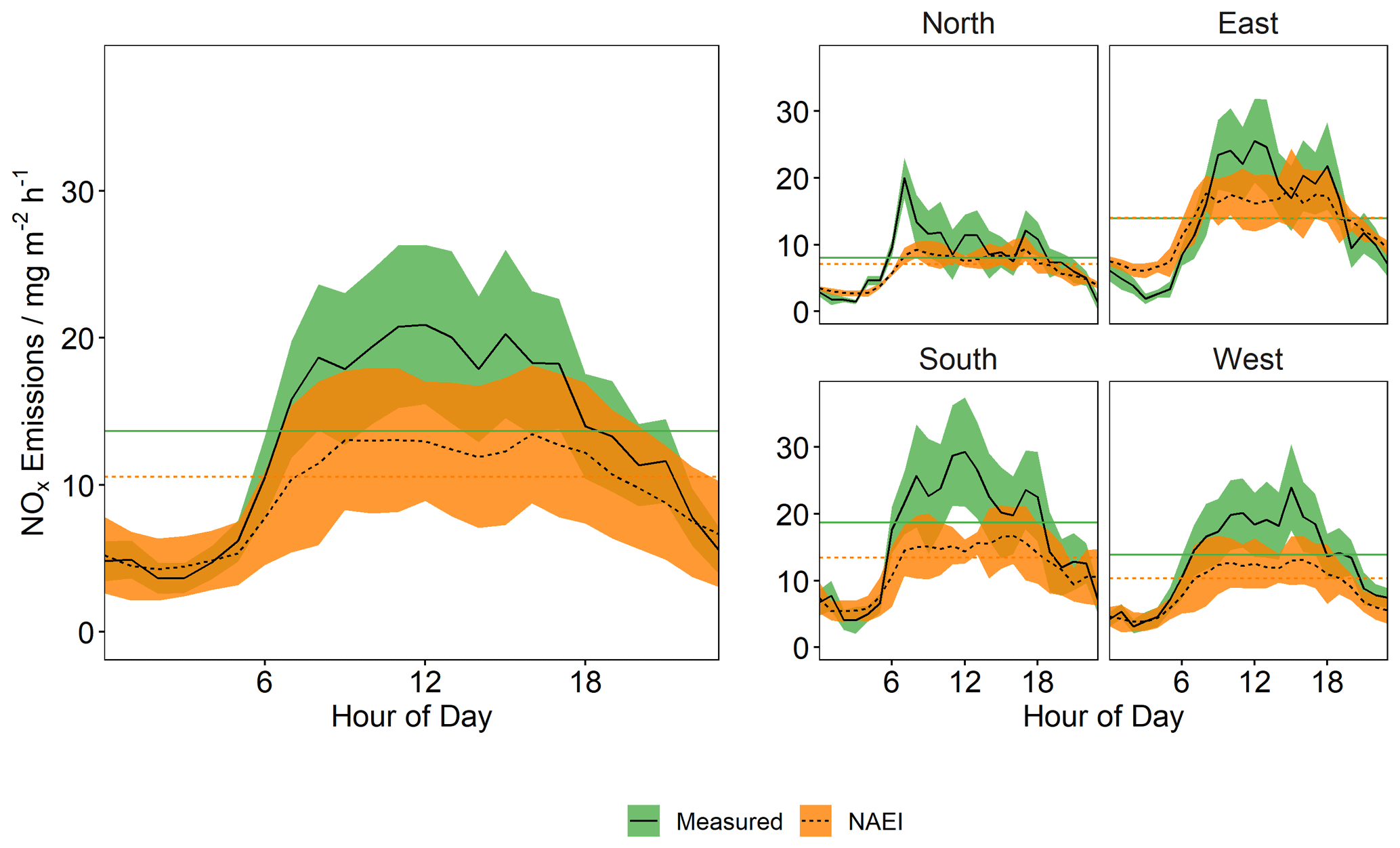
Figure 8 Median diurnal profiles of NO_x emissions measured (green, solid) at the BT Tower in March–July 2017 and simulated emissions from the NAEI (orange, dashed). The shaded region shows the total (random + systematic) error in flux measurement for the measured emission and median absolute deviation in diurnal averaging for simulated emissions. The horizontal lines show the daily median values. The left-hand side shows the average diurnal profiles for the total measurement period, and right-hand side shows this separated by wind direction.

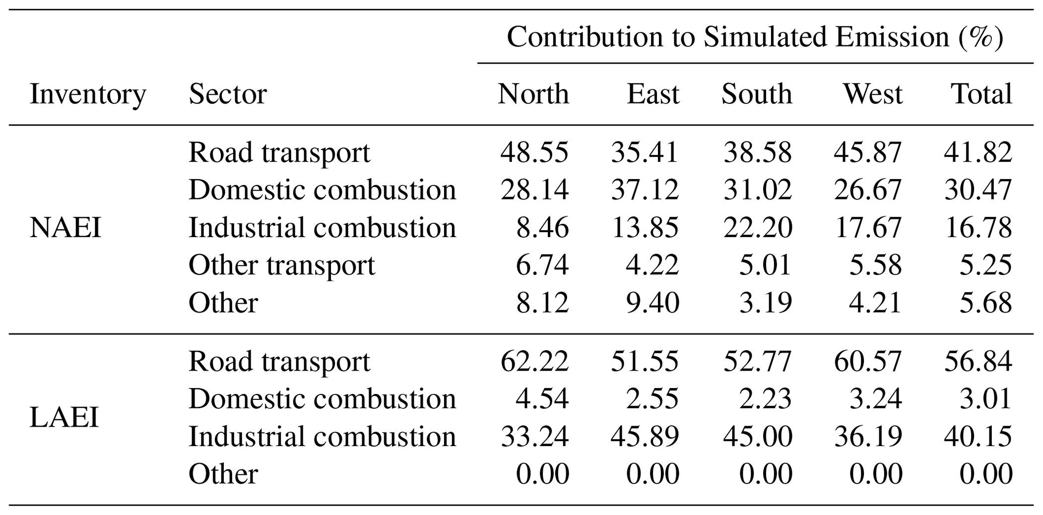
By wind sector the story is more varied. The north and east show the measurements spiking significantly above the simulated emissions during the morning but then show good agreement throughout the rest of the day, again with the simulated emissions being higher at night. This is reflected in the daily medians of both of these sectors being much closer to unity (ratios of 1.13 and 0.99, respectively). In the south and west the daytime underestimation by the inventory can be observed (ratios of 1.54 and 1.53, respectively), whereas overnight the agreement is better than the overall average at 1.03 and 1.00, respectively. Table 2 presents the sector breakdown from the simulated emissions time series to explore whether any particular sector may be responsible for the missing emissions. However, from this there is no stand-out sector responsible for the underestimation.

Table 2 Inventory sector contribution to simulated emissions by wind sector.

In Fig. 9 the diurnal profiles have been separated by day of week. Here the simulated emission is presented by hourly bars separated by source sector and is additionally presented alongside the average traffic volume measured at 24 automatic traffic counting sites, selected from those that occupied grid cells making up the first 80 % of the contribution to the flux footprint climatology. The primary diurnal variation in the simulated emissions comes from the road transport and combustion sectors, and here it can been see to be driving the double peak during the day. Diurnally, the road transport sector follows the measured traffic volumes, as this is driven by the diurnal scaling factor, and for the weekday/weekend, the difference is again driven by the day of week scaling factor. The effect of the latter can be seen more clearly in Fig. 10, where day of week averages of both measured and simulated emissions are presented. Here, decreased agreement between the simulated and measured emissions is seen on Saturday, primarily being driven by the scaling factors decreasing at the weekend (Figs. A3 and A4). From the measurements, Saturday's emissions are much more comparable to the weekdays than Sunday. This may be a property more unique to London. Much of the combustion within the footprint climatology is from commercial combustion – as demonstrated by the domestic combustion sector being significantly diminished in the LAEI, which groups commercial combustion into the industrial combustion sector. Commercial sources would be expected to continue activity on a Saturday, which, coupled with limited reductions in average traffic flow, could explain why this behaviour may be more unique to central London and is therefore less well captured by general scaling factors.

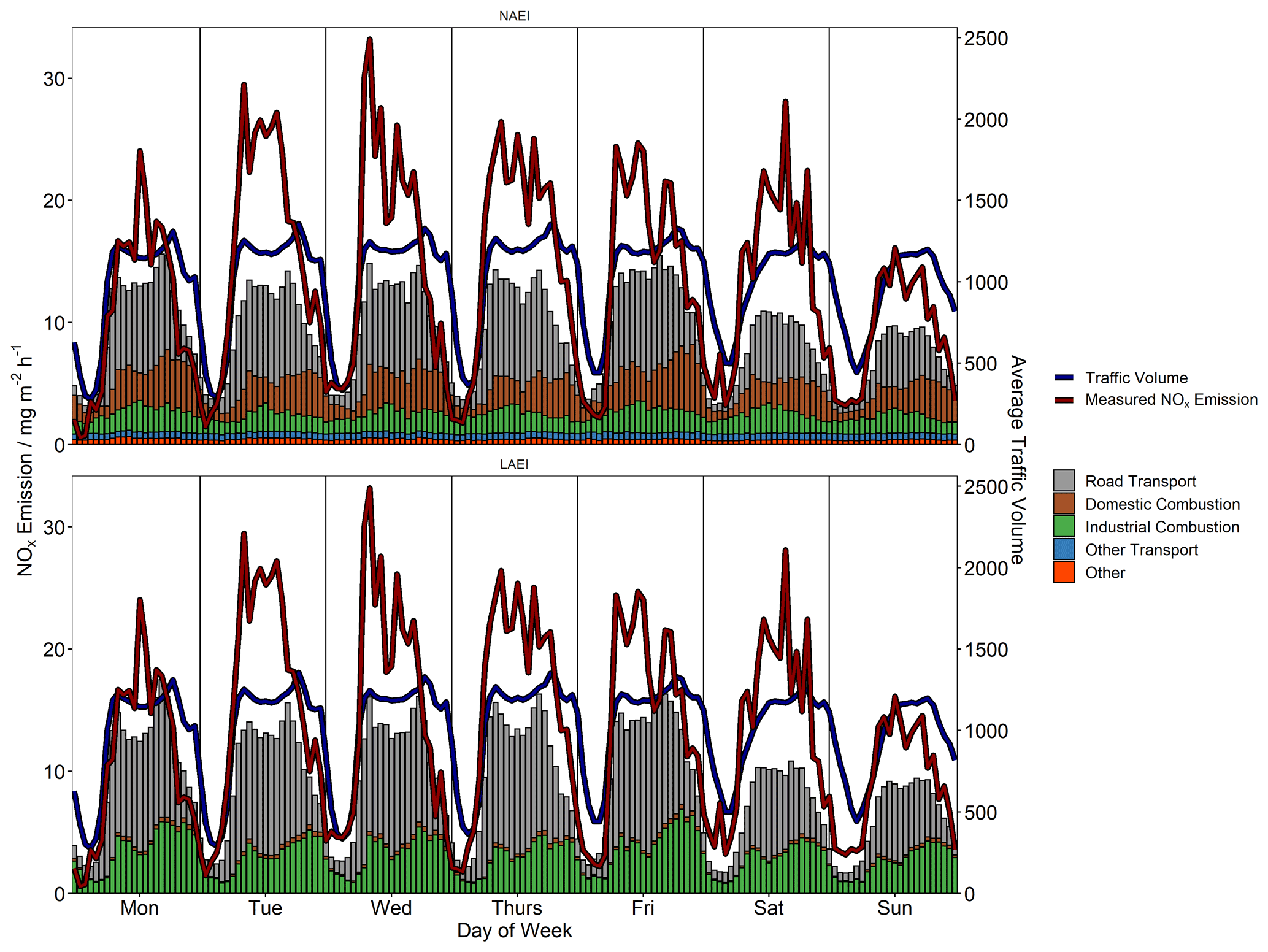
Figure 9 Average diurnal profiles of NO_x emissions measured (red) at the BT Tower in March–July 2017 and the NAEI's estimated emission (bars) from within the flux footprint, separated by day of week. NAEI emissions are coloured by source sector contribution. Median traffic volume from 24 automatic traffic counters surrounding the site is shown in blue.

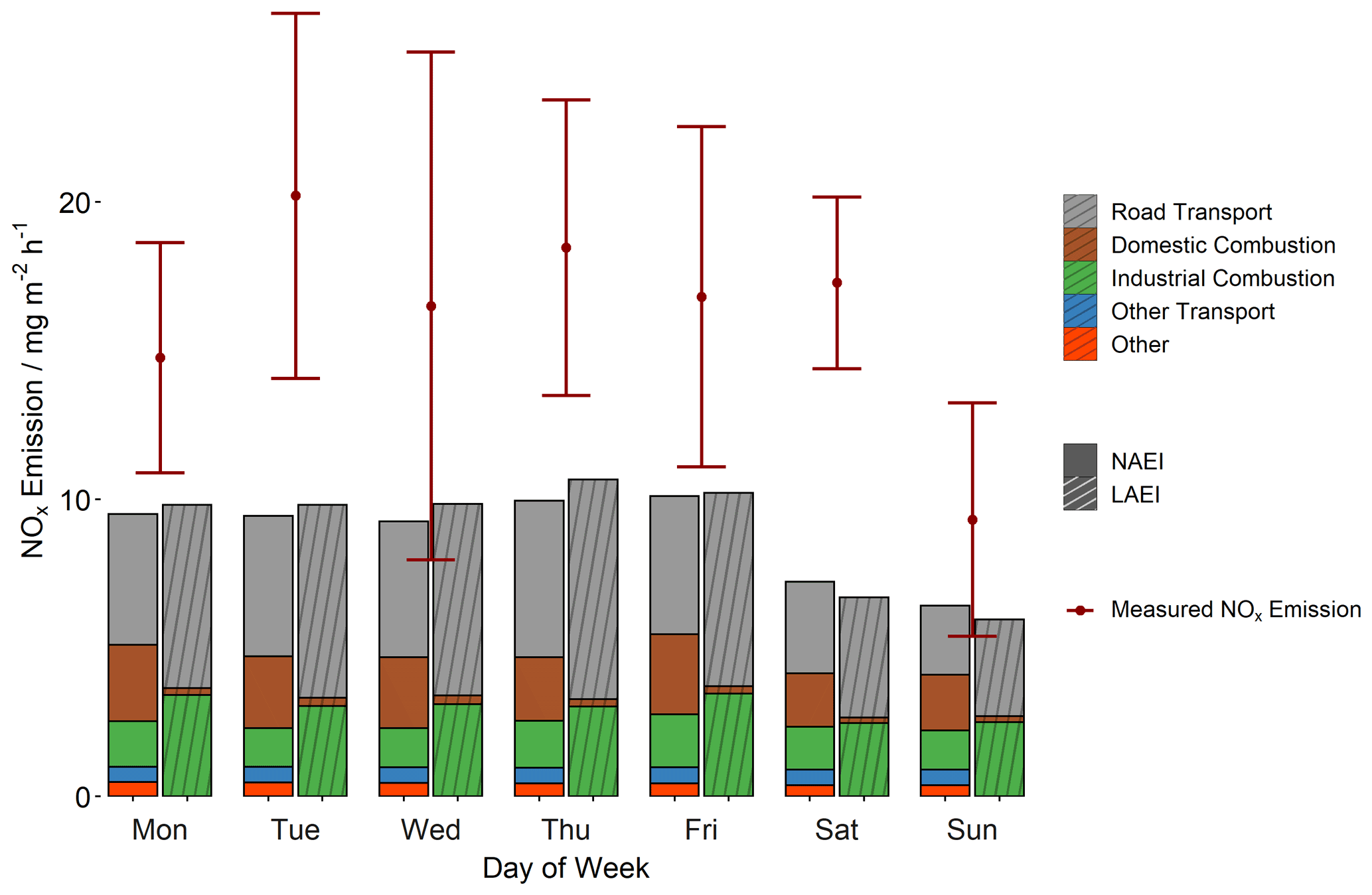
Figure 10 Daily averaged measured NO_x emissions by day of week shown as red points and stacked bars of simulated emissions coloured by source sector for the NAEI (solid colour) and LAEI (hatched).

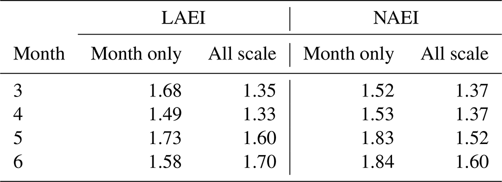
A budget closure type of exercise was also conducted to probe the effect different degrees of scaling have on the measurement to inventory ratio. This was done by constructing the simulated inventory time series as previously described along with a second series wherein only the monthly scaling factors were applied. Both of these, along with the measurement time series, were averaged by month, the assumption being that the hourly or weekly scaling factors should be mostly averaged out over the course of a month, as they sum to unity over 24 h or 7 d, respectively. This assumption is perturbed by the uneven sampling across the diurnal profile, with ∼ 3 times more missing values overnight, driven by processes such as stationarity violations (“Night-time stationarity” section). This is reflected in the comparison in Table 3 where only using monthly factors leads to underestimates that are generally larger than when all scaling factors are used, driven by the daytime scaling factors increasing the values, without their night-time counterparts. These underestimates (1.37–1.84 for the NAEI and 1.35–1.73 for the LAEI) are similar to the daytime underestimates presented earlier, reinforcing the idea that there are missing sources of NO_x within the flux footprint climatology surrounding the BT Tower and not simply an artefact from the emissions simulation method.

Table 3 Ratio of measured to simulated NO_x emissions from both the NAEI and the LAEI. For each inventory the cases for both all scaling factors and only monthly scaling factors are shown.

To further explore the differences in wind sector dependence of the emissions and begin to identify potential missing sources, Fig. 11 shows daytime and night-time average emissions by 22.5^∘ wind direction bins. The daytime underestimation is sustained through the western and southern direction, whereas the underestimation that manifested as a morning peak in the north and east diurnals is much narrower. It can also be seen that to the north-west the simulated emissions agree or even slightly overestimate versus the measurements. Overnight the agreement improves in all directions.

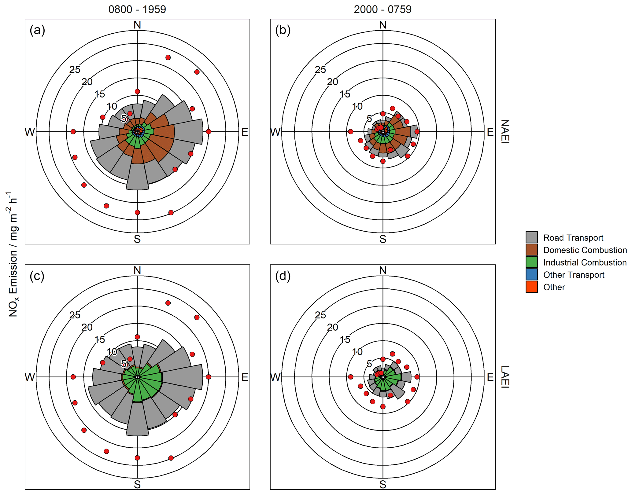
Figure 11 NO_x emissions (red) measured at the BT Tower in March–July 2017 and the NAEI's estimated emission (bars) from within the flux footprint, averaged by 22.5^∘ wind sector bins. NAEI emissions are coloured by source sector contribution. The left-hand panel shows all data between 08:00 and 19:59, and the right-hand panel shows all data between 20:00 and 07:59.

In Fig. 12, the surface mapping approach, as described in Sect. 2.3.3, has been applied to the measured and simulated (NAEI) emissions in an attempt to further elucidate the spatial discrepancies observed here. The measured flux is mapped in panel (a) and the simulated inventory time series in panel (b); the difference between these is shown in panel (c). Areas to the north-east, south, and west that have been highlighted by the measurements as significant sources are not captured by the inventory in this treatment, revealing sources that are not fully resolved by the inventory. This method of mapping these emissions cannot be easily validated, and by using just along-wind distance to footprint maxima, much of the spatial information is collapsed – however, the same caveats apply to both the measured and simulated maps, and comparison of them may provide some insight into their respective differences.

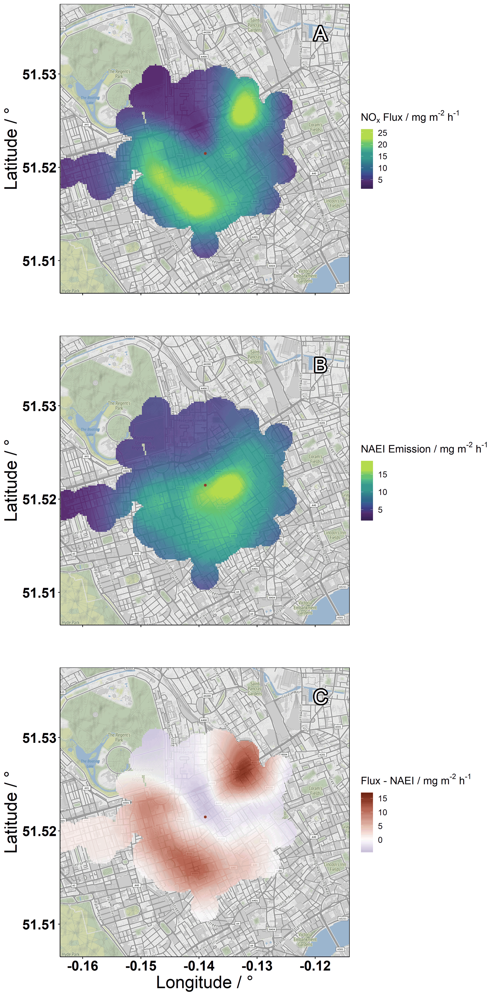
Figure 12 (a) Measured NO_x flux as a function of along-wind distance to the maximum flux contribution on the radius, separated by wind direction. (b)  NAEI NO_x emissions estimate as a function of along-wind distance to the maximum flux contribution on the radius, separated by wind direction. For panels (c–b) subtracted from (a), red shows measurement greater than inventory, and blue shows inventory greater than measurement. Map tiles by Stamen Design, under CC BY 3.0. Data by OpenStreetMap, under ODbL. Tiles accessed via the ggmap R package (Kahle and Wickham, 2013).

The measured emissions (Fig. 12a) place the emission enhancements to the south-west over the areas of Oxford Street and Regents Street, and the enhancement in the north-east is over Euston Station and Marylebone Road. Both of these areas are busy with road transport, and Euston Station also has a bus depot which filters into the already congested Marylebone Road. It is possible that these enhancements are not well captured by the NAEI as they are localised at features much finer than the inventories' spatial resolution (shown by the lack of similar structure in Fig. 12b), and they could also be due to specific driving conditions found on these roads, which will not be well described by a bottom-up approach of inventory construction. The decreased emissions over The Regent's Park to the north-west are again likely due to the resolution of the inventory – though the map being sensitive to this large green space within the footprint provides some qualitative validation of the method.

3.3 Comparison with other urban NO_x emissions measurements

Several other studies have measured urban NO_x flux, and we compare examples from their measurements here for context. When conversion between molar and mass units was required a molecular mass of 38 g mol⁻¹, the mean of NO and NO₂ masses, was used. Marr et al. (2013) measured at multiple sites in Norfolk, Virginia, USA, and surrounding areas (within 12×12 km) using a mobile platform across 92 h in June 2008. They measured a range of magnitudes of NO_x fluxes depending on their particular site location, but the largest measured was comparable to those measured in this study, 39.96 mg m⁻² h⁻¹, from a site situated by an intersection with steady traffic and high proportion of diesel vehicles. They found on average that the inventory they compared with underestimated by 1.9 times. Karl et al. (2017) measured from a tower site in Innsbruck in a valley with significant vehicle transport between July and October 2015. The maximum average in their mid-week diurnal profile was 6.4 mg m⁻² h⁻¹, which is significantly lower. Indeed this study compares with Lee et al. (2015), finding the Innsbruck measurements to be 3–4 times lower than those measured in London. Guidolotti et al. (2017) measured from a tower site in Real Bosco di Capodimonte – a large green area within Naples, Italy. The footprint of this site was influenced by the surrounding green space and showed a maximum NO_x flux of 3.6 mg m⁻² h⁻¹. Vaughan et al. (2016) measured from an airborne platform for 12 flights over 2 weeks in July 2013. They measured in the range of 30–80 mg m⁻² h⁻¹ on flight tracks near central London and found the NAEI to underestimate by around 1.5 times on average. Squires et al. (2020) measured from a tower site in central Beijing for several weeks during the winter 2016 and summer 2017. The average emission for these periods was 4.4 and 3.6 mg m⁻² h⁻¹, respectively. Here they found the inventory to overestimate measured NO_x by 7 times. This places our measurements of NO_x flux on similar ground as those measured in similar urban environments, and measurements made in London suggest that NO_x emission has not decreased substantially in the intervening time since the studies by Lee et al. (2015) and Vaughan et al. (2016). To highlight this we have recalculated the fluxes measured by Lee et al. (2015) in 2013 using the same processing method described here and also generated an inventory comparison using a 2012 version of the NAEI (Fig. 13). The daytime fluxes from Lee et al. (2015) are slightly higher than those measured in this study, and the simulated NAEI emissions are also slightly higher – but the difference is well within the flux uncertainty for both periods.

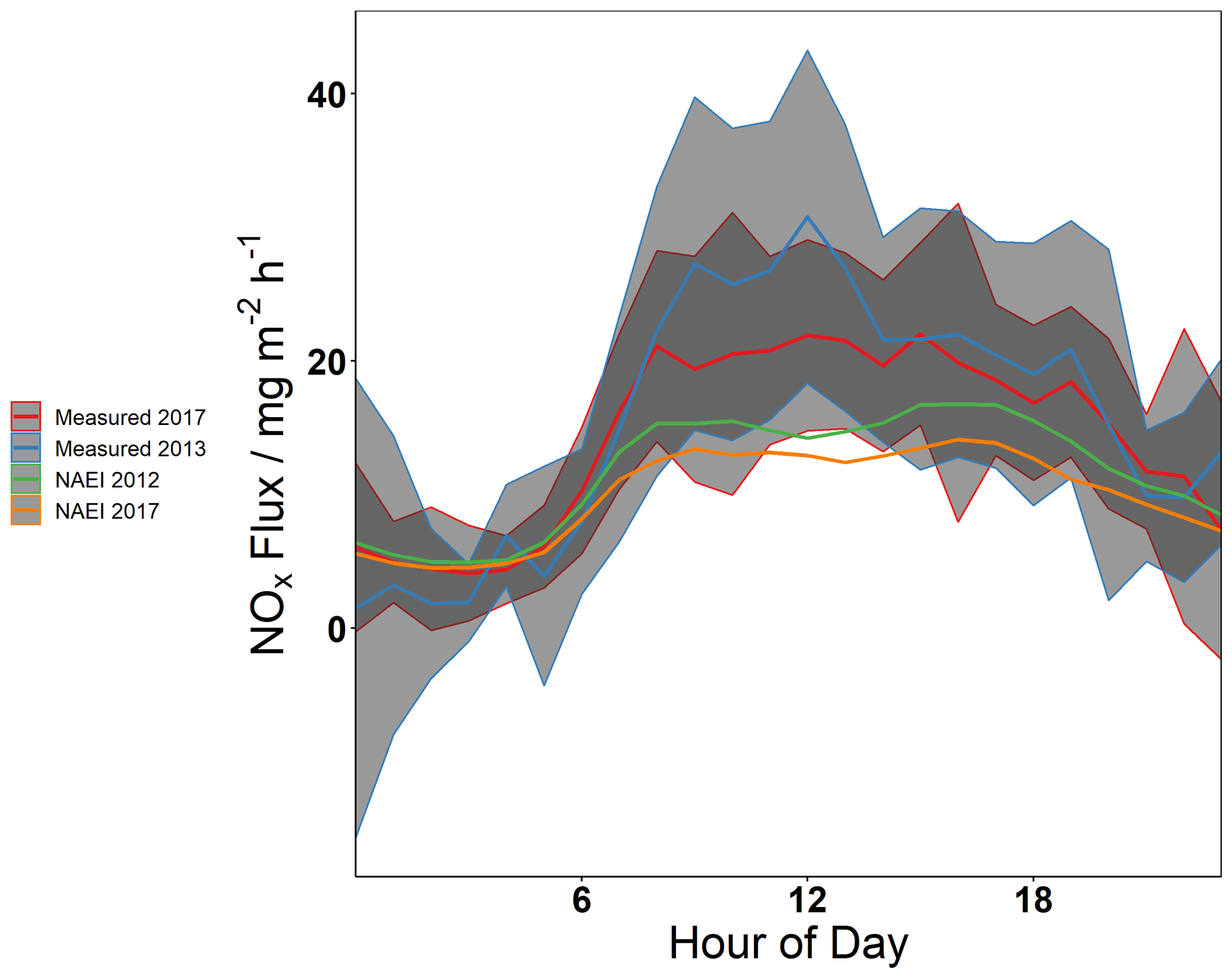
Figure 13 Diurnal profiles of measured NO_x flux in 2013 (blue, recalculated from Lee et al., 2015) and 2017 (red, this study) compared with inventory time series generated from 2012 (green) and 2017 (orange) versions of the NAEI.

4 Conclusions

During March–June 2017 NO_x flux was measured at the BT Tower in central London via eddy covariance. A footprint model was used to simulate an emissions time series from the spatially resolved NAEI and LAEI. This work also discussed some of the challenges of making eddy covariance measurements at this site – many of which are applicable to other urban eddy covariance sites. Methods are now in place for more sufficiently quantifying the high-frequency loss of the system deployed at the site and for analyses wherein these losses may be more important – such as cases in which inventories have been revised and now overestimate relative to measurements – they should be applied more routinely. This study has begun to explore the flux loss from vertical divergence but cannot yet firmly conclude on a correction method. There is, as of 2020, long-term data collection of NO_x fluxes at the site, and the primary use of these should be to further this analysis.

The inventories underestimated (1.48 times) the measured NO_x emissions during the day but showed improved agreement overnight. This underestimation was present in monthly averaged comparisons also (1.35–1.84 times). Using the footprint model again, spatial differences in the measured and simulated emissions were explored, and using this method it appeared that particularly congested regions around the tower were not well represented by the inventory.

It is clear from these measurements that there are contributions to the NO_x emission in central London not captured by the inventory; however, they do not allow us to untangle their sources explicitly. While this is currently the longest time series of measured NO_x emission in the city, 3–4 months of data necessitates the use of scaling factors to make comparisons with the inventories. The monthly averaged comparison shows that the underestimation is not a factor of this process alone, but the day of week comparison shows flaws in the use of these factors that are generalised across anthropogenic activity – the activity of central London may not be reflected precisely by them. Collection of a time series spanning more than 12 months would allow annual budgets to be compared (and ongoing data collection will provide this in future work). Although a difference between the measured and inventory emissions is likely to persist, a single annual data point will do little to untangle the source of this discrepancy. So in many cases, the ability to produce high-temporal-resolution emissions estimates will still be necessary, and provision of this information from inventory constructors would improve the comparisons that can be made. Indeed the LAEI used here provided hourly scaling for the road transport sector – but this does not yet provide sufficient information when it is mixed with the other required factors.

Resolving the measurements spatially does provide hints as to where the discrepancies may be found, and here we showed that the highest emissions around the tower were close to locations that experience high congestion. The change in traffic emissions due to congestion is not something that is directly parameterised in the bottom-up inventories used here, but further investigation may be able to close the gap between them and measurements.

Continued policy intervention in London, such as the implementation and expansion of the ultra-low emission zone as well as changes in short-term activity and long-term behaviours resulting from the COVID-19 pandemic which took hold in the UK in March 2020, will strongly affect NO_x emissions in London. Improvements in emissions inventories using measurements such as these will provide a more accurate baseline to assess those changes, as will using ongoing measurements to further validate how the inventories adapt to and implement these changes.

Appendix A

Figure A1 Schematic eddy covariance calculation workflow.

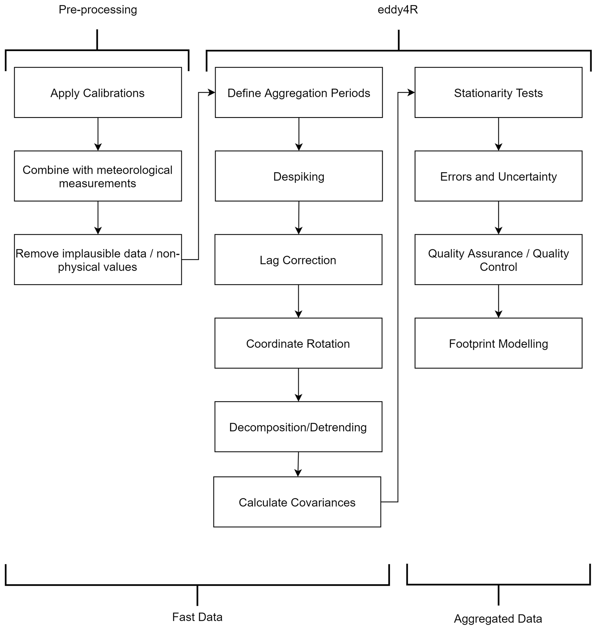
Table A1 SNAP (Selected Nomenclature for sources of Air Pollutants) sector definitions as used in the NAEI Defra and BEIS (2017). The four sectors with the largest contribution to NO_x emissions within the footprint of the BT Tower are highlighted in bold.

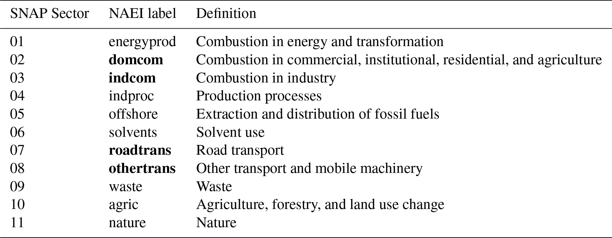
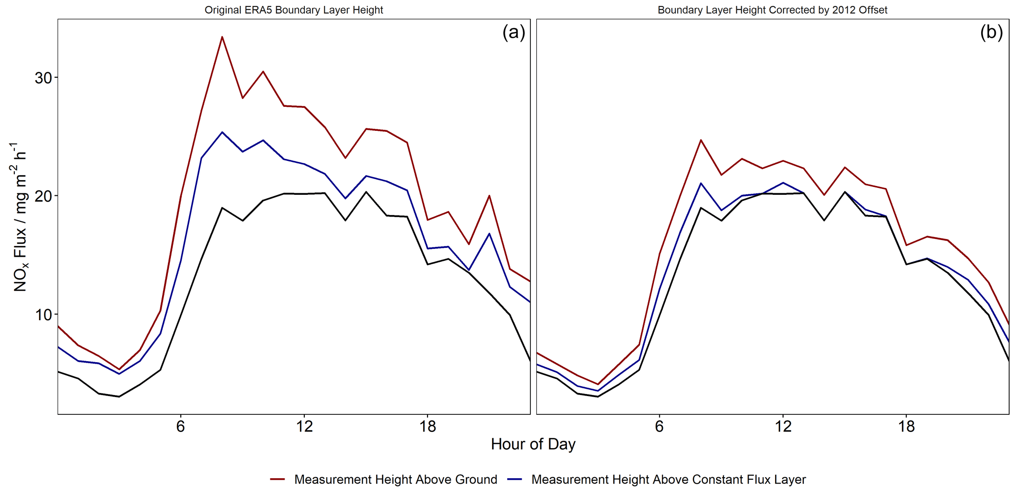
Figure A2 Visualisation of the vertical flux divergence corrections with respect to boundary layer height. (a) Corrected NO_x flux against uncorrected NO_x flux, coloured by boundary layer height. (b) Correction factor against boundary layer height.

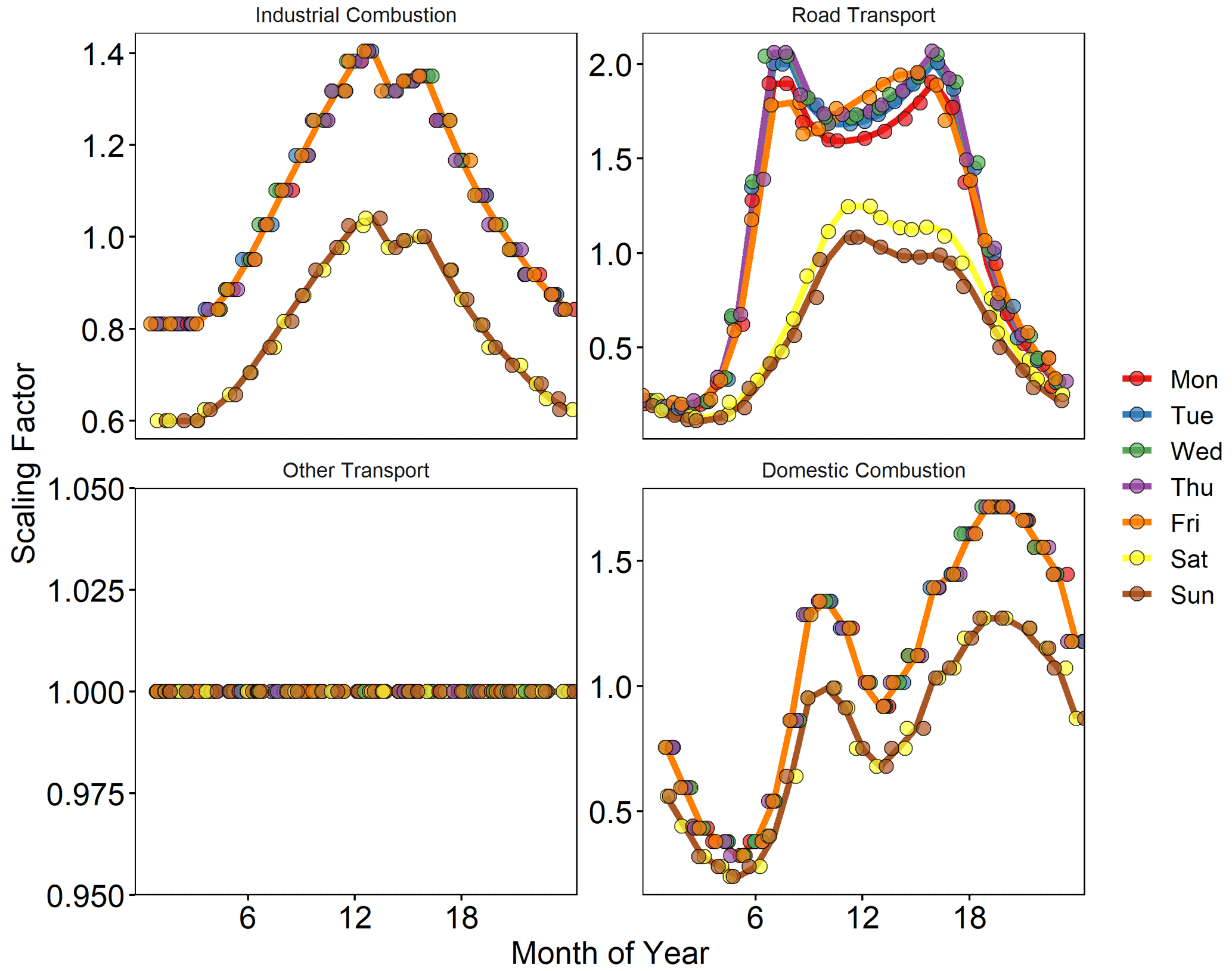
Figure A3 Hour of day scaling factors for the four SNAP sectors (07, 02, 03, and 08, see Table A1) contributing to the majority of NO_x emissions around the BT Tower, coloured by day of week. Overlapping points for identical profiles have been offset in the x direction to improve readability.

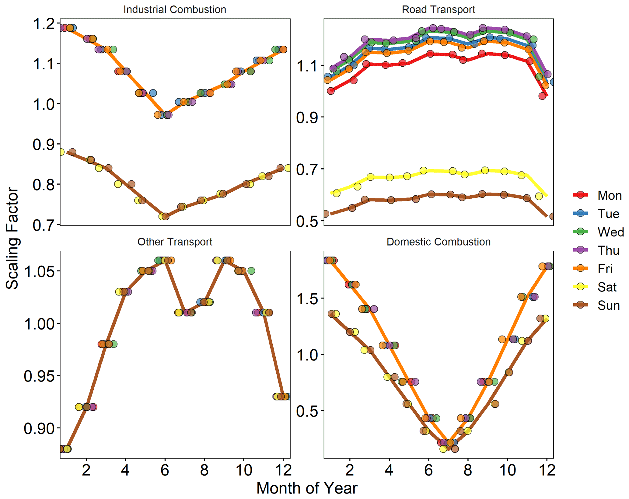
Figure A4 Month of year scaling factors for the four SNAP sectors (07, 02, 03, and 08, see Table A1) contributing to the majority of NO_x emissions around the BT Tower, coloured by day of week. Overlapping points for identical profiles have been offset in the x direction to improve readability.