Examination of aerosol impacts on convective clouds and precipitation in two metropolitan areas in East Asia; how varying depths of convective clouds between the areas diversify those aerosol effects?

This study examines the role played by aerosols which act as cloud condensation nuclei (CCN) in the development of clouds and precipitation in two metropolitan areas in East Asia that have experienced substantial increases in aerosol concentrations over the last decades. These two areas are the Seoul and Beijing areas and the examination was done by performing simulations using the Advanced Research Weather Research and Forecasting model as a cloud system resolving model. The CCN are advected from the continent to the Seoul area and this increases aerosol concentrations in the Seoul area. These increased CCN concentrations induce the enhancement of condensation that in turn induces the enhancement of deposition and precipitation amount in a system of less deep convective clouds as compared to those in the Beijing area. In a system of deeper clouds in the Beijing area, increasing CCN concentrations also enhance condensation but reduce deposition. This leads to negligible CCN-induced changes in the precipitation amount. Also, in the system there is a competition for convective energy among clouds with different condensation and updrafts. This competition results in different responses to increasing CCN concentrations among different types of precipitation, which are light, medium and heavy precipitation in the Beijing area. The CCN-induced changes in freezing play a negligible role in CCN-precipitation interactions as compared to the role played by CCN-induced changes in condensation and deposition in both areas.

1 Introduction

With increasing aerosol loading or concentrations, cloud particle sizes can be changed. In general, with increasing droplet sizes the efficiency of collision and collection among droplets increases. Increasing aerosol loading is known to make the droplet size smaller and thus make the efficiency of collision and collection among droplets lower. This leads to less droplets or cloud liquid forming raindrops and there is more cloud liquid present in the air to be evaporated or frozen. Studies have shown that increases in cloud liquid mass due to increasing aerosol loading can enhance the freezing of cloud liquid and parcel buoyancy, which lead to the invigoration of convection (Rosenfeld et al., 2008; Fan et al., 2009). Via the invigoration of convection, precipitation can be enhanced. The dependence of aerosol-induced invigoration of convection and precipitation enhancement on aerosol-induced increases in condensational heating in the warm sector of a cloud system has been shown (e.g., van den Heever et al., 2006; Fan et al., 2009; Lee et al., 2018). Increasing cloud liquid mass induces increasing evaporation, which intensifies gust fronts. This in turn strengthens convective clouds and increases the amount of precipitation (Khain et al., 2005; Tao, 2007; Storer et al., 2010; Tao et al., 2012; Lee et al., 2017, 2018). It is notable that aerosol-induced precipitation enhancement is strongly sensitive to cloud types that can be defined by cloud characteristics, such as cloud depth (e.g., Tao, 2007; Lee et al., 2008; Fan et al., 2009).

Since East Asia was industrialized, there have been substantial increases in aerosol concentrations over the last decades in East Asia (e.g., Lee et al., 2013; Lu et al., 2011; Oh et al., 2015; Dong et al., 2019). These increases are far greater than those in other regions, such as North America and Europe (e.g., Lu et al., 2011; Dong et al., 2019). While the increasing aerosols affect clouds, precipitation and hydrologic circulation in continental East Asia, the increase in the advected aerosols from the continent to the Korean Peninsula affects clouds, precipitation and hydrologic circulation in the Korean Peninsula (Kar et al., 2009). This study aims to examine the effects of the increasing aerosols, which particularly act as cloud condensation nuclei (CCN), and their advection on clouds and precipitation in East Asia. This study focuses on aerosols which act as CCN but not ice-nucleating particles (INPs) to examine these effects, based on the fact that CCN account for most of the aerosol mass that affects clouds and precipitation, and CCN, but not INPs, are associated with the described aerosol-induced invigoration of convection and intensification of gust fronts. Note that the aerosol-induced invigoration and intensification are two well-established major theories of aerosol-cloud interactions. As a first step to the examination, this study focuses on two metropolitan areas in East Asia which are the Beijing and Seoul areas. The population of each of the Beijing and Seoul areas is ∼20 million. Associated with this, these areas have many of aerosol sources (e.g., traffic) and have made a substantial contribution to the increases in aerosol concentrations in East Asia. Hence, we believe that these two cities can represent the overall situation related to increasing aerosol concentrations in East Asia.

As mentioned above, aerosol-cloud interactions (and their impacts on precipitation) are strongly dependent on cloud types and thus to gain a more general understanding of those interactions, we select cases from the Beijing and Seoul areas with different cloud types. A selected case from the Beijing area involves deep convective clouds that reach the tropopause, while a selected case from the Seoul area involves comparatively shallow (or less deep) convective clouds. Via comparisons between these two cases, we aim to identify mechanisms that control varying aerosol-cloud interactions with cloud types.

To examine the impacts of aerosols, which act as CCN, on clouds and precipitation in the cases, numerical simulations are performed as a way of fulfilling the described aim. These simulations use a cloud-system resolving model (CSRM) that has reasonably high resolution to resolve cloud-scale processes related to cloud microphysics and dynamics. Hence, these simulations are able to find process-level mechanisms in association with cloud-scale processes.

2 Case description

In the Seoul area, South Korea, there was an observed mesoscale convective system (MCS) for a period from 03:00 LST (local solar time) to 18:00 LST on 24 December 2017. During this period, there was a recorded moderate amount of precipitation and its maximum precipitation rate reached ∼13 mm h⁻¹. Here, precipitation in the Seoul area was measured by rain gauges in automatic weather stations (AWSs) (King, 2009). The measurements were performed hourly with a spatial resolution that ranges from ∼1 to ∼10 km. The Seoul area is marked by an inner rectangle in Fig. 1a and dots in the rectangle in Fig. 1a mark the selected locations of rain gauges. At 21:00 LST on 23 December 2017, synoptic-scale features developed in favor of the formation and development of the selected MCS and associated moderate rainfall. These features involved the southwesterly low-level jets that transport warm and moist air to the Korean Peninsula. The southwesterly low-level jet plays an important role in the formation and development of rainfall events in the Korean Peninsula by fetching warm and moist air (Hwang and Lee, 1993; Lee et al., 1998; Seo et al., 2013; Oh et al., 2018).

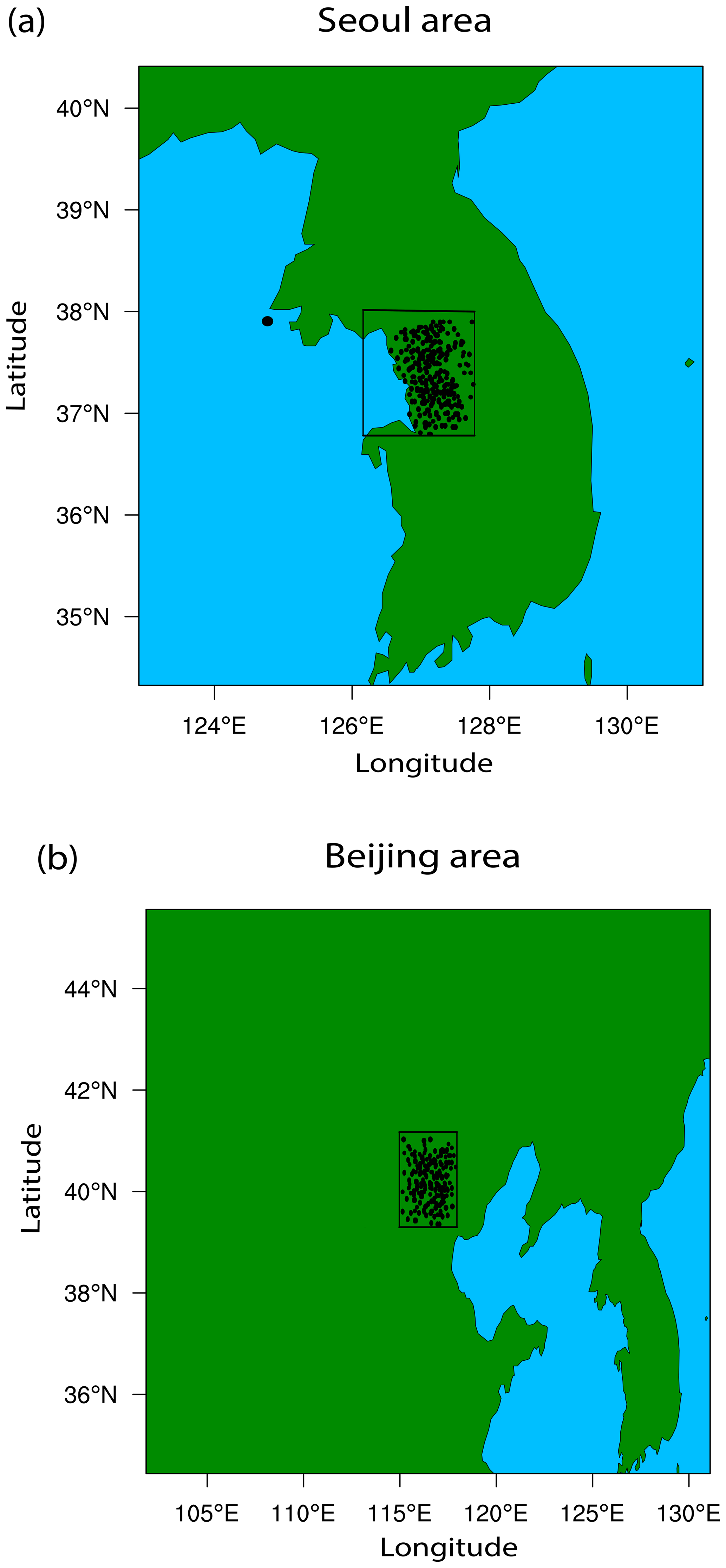
Figure 1 Inner rectangles in (a) and (b) mark the Seoul area in the Korean Peninsula and the Beijing area in the East Asia continent, respectively. A dot outside the inner rectangle in (a) marks Baekryongdo island. Dots in the inner rectangles in (a) and (b) mark the selected locations where precipitation and aerosol mass are measured. In (a) and (b), the light blue represents the ocean and the green the land area.

There was another observed MCS case in the Beijing area, China for a period from 14:00 LST on 27 July to 00:00 LST on 28 July 2015. There was a substantial amount of precipitation recorded for this period and its maximum precipitation rate reached ∼45 mm h⁻¹. Here, similar to the situation in the Seoul area, precipitation in the Beijing area was measured by rain gauges in AWSs hourly with a spatial resolution that ranges from ∼1 to ∼10 km. The Beijing area is marked by an inner rectangle in Fig. 1b and dots in the rectangle in Fig. 1b mark the selected locations of rain gauges. At 09:00 LST 27 July 2015, synoptic-scale features developed in favor of the formation and development of the selected MCS. These features involved the southerly low-level jet that developed heavy rainfall events in the Beijing area by transporting warm and moist air to the area. Synoptic features which are described here are based on reanalysis data that are produced by the Met Office Unified Model (Brown et al., 2012) every 6 hours with a $\mathrm{0.11}{}^{\circ }\times \mathrm{0.11}{}^{\circ }$ resolution.

3 CSRM and simulations

3.1 CSRM

The Advanced Research Weather Research and Forecasting (ARW) model (version 3.3.1) is used as a CSRM. The ARW model is a compressible model with a nonhydrostatic status. A 5th order monotonic advection scheme is used to advect microphysical variables (Wang et al., 2009). The Rapid Radiation Transfer Model (RRTM; Mlawer et al., 1997; Fouquart and Bonnel, 1980) is adopted to parameterize shortwave and longwave radiation in simulations. A microphysics scheme that is used in this study calculates the effective sizes of hydrometeors that are fed into the RRTM, and the RRTM simulates how these effective sizes affect radiation.

The CSRM adopts a bin scheme as a way of parameterizing microphysics. The Hebrew University Cloud Model (HUCM) detailed in Khain et al. (2011) is the bin scheme. A set of kinetic equations is solved by the bin scheme to represent a size distribution function for each of seven classes of hydrometeors and aerosols acting as CCN. Hence, there are seven size distribution functions for hydrometeors. The seven classes of hydrometeors are water drops, three types of ice crystals, which are plates, columns and dendrites, snow aggregates, graupel and hail. Drops with a radius smaller (larger) than 40 µm are categorized to be droplets (raindrops). There are 33 bins for each size distribution in a way that the mass of a particle m_j in the j bin is to be $m_j=\mathrm{2}{m}_{j-\mathrm{1}}$.

The parameterization of cloud-droplet nucleation is based on the Köhler theory. Arbitrary aerosol mixing states and aerosol size distributions can be fed into this parameterization. To represent heterogeneous ice-crystal nucleation, parameterizations by Lohmann and Diehl (2006) and Möhler et al. (2006) are used. In these parameterizations, contact, immersion, condensation-freezing, and deposition nucleation paths are all considered by taking into account the size distribution of INPs, temperature and supersaturation. Homogeneous droplet freezing is considered following the theory developed by Koop et al. (2000).

3.2 Control runs

For a three-dimensional CSRM simulation of the observed case of convective clouds in the Seoul (Beijing) area, i.e., the control-s (control-b) run, a domain just over the Seoul (Beijing) area, which is shown in Fig. 1a (1b), is used. This domain adopts a 300 m resolution. The control-s run is for a period from 03:00 to 18:00 LST on 24 December 2017, while the control-b run is for a period from 14:00 LST on 27 July to 00:00 LST 28 July 2015. The length of the domain is 170 (140) km in the east–west (north–south) direction for the control-s run, and 280 (240) km for the control-b run. There are 100 vertical layers and these layers employ a sigma coordinate that follows the terrain. The top pressure of the model is 50 hPa for both of the control-s and control-b runs. On average, the vertical resolution is ∼200 m.

Reanalysis data, which are produced by the Met Office Unified Model (Brown et al., 2012), represent the synoptic scale features, provide initial and boundary conditions of variables, such as wind, potential temperature, and specific humidity for the simulations. The simulations adopt an open lateral boundary condition. The Noah land surface model (LSM; Chen and Dudhia, 2001) calculates surface heat fluxes.

The current version of the ARW model is not able to consider the spatiotemporal variation of aerosol properties. In order to take into account the spatiotemporal variation of aerosol properties, which is typical in metropolitan areas, such as composition and number concentration, an aerosol preprocessor, which is able to consider the variability of aerosol properties, is developed and used in the simulations. This aerosol preprocessor interpolates or extrapolates background aerosol properties in observation data such as aerosol mass (e.g., PM_2.5 and PM₁₀) into grid points and time steps in the model. In this study, the inverse distance weighting method is used for the extrapolation and interpolation of observation data including aerosol mass into grid points and time steps in the model. PM stands for particulate matter. The mass of aerosols with diameter smaller than 2.5 (10.0) µm per unit volume of the air is PM_2.5 (PM₁₀).

There are surface observation sites, which measure aerosol properties in the domains and these sites are classified into two types; the selected locations of these sites are marked by dots in the inner rectangles in Fig. 1. The distance between the observation sites ranges from ∼1 to ∼10 km and the time interval between observations is ∼10 min. More than 90 % of the sites belong to the first type of sites. These first type sites are managed by the government in South Korea or China, and measure PM_2.5 or PM₁₀ but not other aerosol properties, such as aerosol composition and size distributions. Less than 10 % of the sites belong to the second type of sites. These second type sites are a part of an aerosol robotic network (AERONET; Holben et al., 2001) and measure aerosol composition and size distributions. The production of aerosol data in these second type or AERONET sites is viable only in the presence of the sun. The first type sites observe PM_2.5 or PM₁₀ using the beta-ray attenuation method (Eun et al., 2016; Ha et al., 2019) and hence, produce PM_2.5 or PM₁₀ data whether the sun is present or not. PM${}_{\mathrm{2.5}}/$PM₁₀ data from the first type sites are used to represent the spatiotemporal variability of aerosols over the domains and the simulation periods. To represent aerosol composition and size distributions, data from the AERONET sites are employed.

The AERONET data are averaged over the AERONET sites at 02:00 LST on 24 December 2017 (13:00 LST on 27 July 2015), which is 1 hour before the observed MCS forms for the Seoul (Beijing) case. Based on the average data it is assumed that aerosol particles are internally mixed with 70 (80) % ammonium sulfate and 30 (20) % organic compounds for the Seoul (Beijing) case. This mixture is assumed to represent the aerosol chemical composition in the whole domain and during the entire simulation period. As ammonium sulfate and organic compounds are representative components of CCN, it is assumed that PM_2.5 and PM₁₀, which are from the first type sites, represent the mass of aerosols that act as CCN for the Seoul and Beijing areas, respectively. Aerosols reflect, scatter and absorb shortwave and longwave radiation before they are activated. This type of aerosol-radiation interaction is not taken into account in this study. This is mainly based on the fact that in the mixture, there are insignificant amounts of radiation absorbers; black carbon is a representative radiation absorber. The average AERONET data indicate that the size distribution of background aerosols acting as CCN follows the bimodal log-normal distribution for both the Seoul and Beijing cases. Based on the average AERONET data, it is assumed that for the whole domain and simulation period, the size distribution of background aerosols acting as CCN follows a shape of distribution with specific size distribution parameters (i.e., modal radius and standard deviation of each of accumulation and coarse modes, and the partition of aerosol number among those modes) for each of the cases. The modal radius of the shape of distribution is 0.110 (0.085) and 1.413 (1.523) µm, while the standard deviations of the shape of distribution are 1.54 (1.63) and 1.75 (1.73) for accumulation and coarse modes, respectively, in the Seoul (Beijing) case. The partition of aerosol number, which is normalized by the total aerosol number of the size distribution, is 0.999 and 0.001 for accumulation and coarse modes, respectively, in both of cases. By using PM_2.5 or PM₁₀, which is not only from the first type sites but also interpolated and extrapolated to grid points immediately above the surface and time steps, and based on the assumption of aerosol composition and size distribution above, which is in turn based on data from the AERONET sites, the background number concentrations of aerosols acting as CCN are obtained for the simulation for each of the cases. There is no variation with height in background concentrations of aerosols acting as CCN from immediately above the surface to the top of the planetary boundary layer (PBL). However, it is assumed that they decrease exponentially with height from the PBL top upward. With this exponential decrease, when the altitude reaches the tropopause, background concentrations of aerosols acting as CCN are reduced by a factor of ∼10 as compared to those at the PBL top. The size distribution and composition of aerosols acting as CCN do not vary with height. Once background aerosol properties (i.e., aerosol number concentrations, size distribution and composition) are put into each grid point and time step, those properties at each grid point and time step do not change during the course of the simulations.

For the control-s and control-b runs, aerosol properties of INPs are not different from those of CCN except for the fact that the concentration of background aerosols acting as CCN is 100 times higher than the concentration of background aerosols acting as INPs at each time step and grid point, following a general difference between CCN and INPs in terms of their concentrations (Pruppacher and Klett, 1978).

Once clouds form and background aerosols start to be in clouds, those aerosols are not background aerosols anymore and the size distribution and concentrations of those aerosols begin to evolve through aerosol sinks and sources that include advection and aerosol activation (Fan et al., 2009). For example, once aerosols are activated, they are removed from the corresponding bins of the aerosol spectra. In clouds, after aerosol activation, the aerosol mass starts to be inside hydrometeors and via collision-collection, it transfers to different types and sizes of hydrometeors. In the end, the aerosol mass disappears in the atmosphere when hydrometeors with aerosol mass touch the surface. In non-cloudy areas, aerosol size and spatial distributions are designed to be identical to the size and spatial distributions of background aerosols, respectively. In other words, for this study, we use the aerosol recovery method. In this method at any grid point, immediately after clouds disappear entirely, aerosol size distributions and number concentrations recover to background properties that background aerosols at those points had before those points are included in clouds. In this way, we can keep concentrations of background aerosols outside clouds in the simulations at observed counterparts. This enables the spatiotemporal distributions of background aerosols in the simulations to mimic those distributions that are observed and particularly associated with observed aerosol advection in reality. In the aerosol recovery method, there is no time interval between the cloud disappearance and the aerosol recovery. When the sum of the mass of all types of hydrometeors (i.e., water drops, ice crystals, snow aggregates, graupel and hail) is not zero at a grid point, that grid point is considered to be in clouds. When this sum becomes zero, clouds are considered to disappear. Many studies using CSRM have employed this aerosol recovery method. They have proven that with the recovery method, reasonable simulations of overall cloud and precipitation properties are accomplished (e.g., Morrison and Grabowski, 2011; Lebo and Morrison, 2014; Lee et al., 2016, 2018).

3.3 Additional runs

We repeat the control-s run by getting rid of aerosol advection-induced increases in concentrations of aerosols acting as CCN as a way of investigating how the aerosol advection affects the cloud system in the Seoul area. This repeated run is named the low-aerosol-s run. An aerosol layer, which is advected from East Asia or from the west of the Seoul area to it, increases aerosol concentrations in the Seoul area. There are stations in islands in the Yellow Sea that monitor the aerosol advection (Eun et al., 2016; Ha et al., 2019). To monitor and identify the aerosol advection, PM_2.5 which is measured by a station in Baekryongdo island in the Yellow Sea is compared to those which are measured in stations in and around the Seoul area. In Fig. 1a, a dot outside the inner rectangle marks the island. The time evolution of PM_2.5 measured by the station on the island and the average PM_2.5 over stations in the Seoul area, between 07:00 LST on 22 December and 21:00 LST on 24 December 2017 when there is the strong advection of aerosols from East Asia to the Seoul area, is shown in Fig. 2. At 09:00 LST on 22 December, the advection of aerosols from East Asia enables the aerosol mass to start going up and attain its peak around 05:00 LST on 23 December on the island. Following this, the aerosol mass starts to increase in the Seoul area around 01:00 LST on 23 December, and the mass attains its peak at 15:00 LST on 23 December in the Seoul area. This is because aerosols, which are advected from East Asia, move through the island to reach the Seoul area.

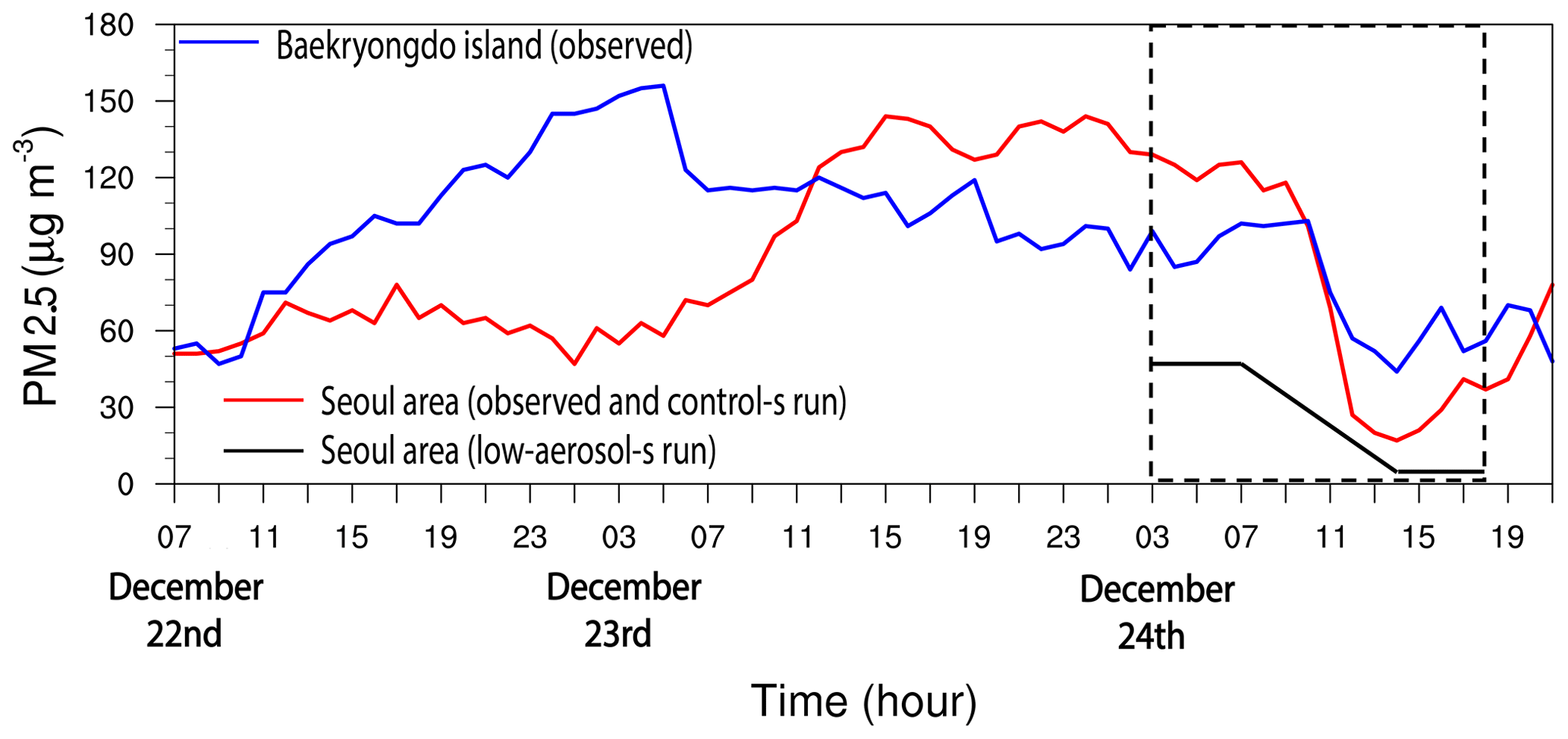
Figure 2 Time series of PM_2.5 observed at the ground station in Baekryongdo island (blue line) and of the average PM_2.5 over ground stations in the Seoul area (red line) between 07:00 LST on 22 December and 21:00 LST on 24 December 2017. Note that PM_2.5 observed at stations in the Seoul area is applied to the control-s run whose period is marked by the dashed rectangle. Time series of the average PM_2.5 over stations in the Seoul area in the low-aerosol-s run for the simulation period is also shown (solid black line).

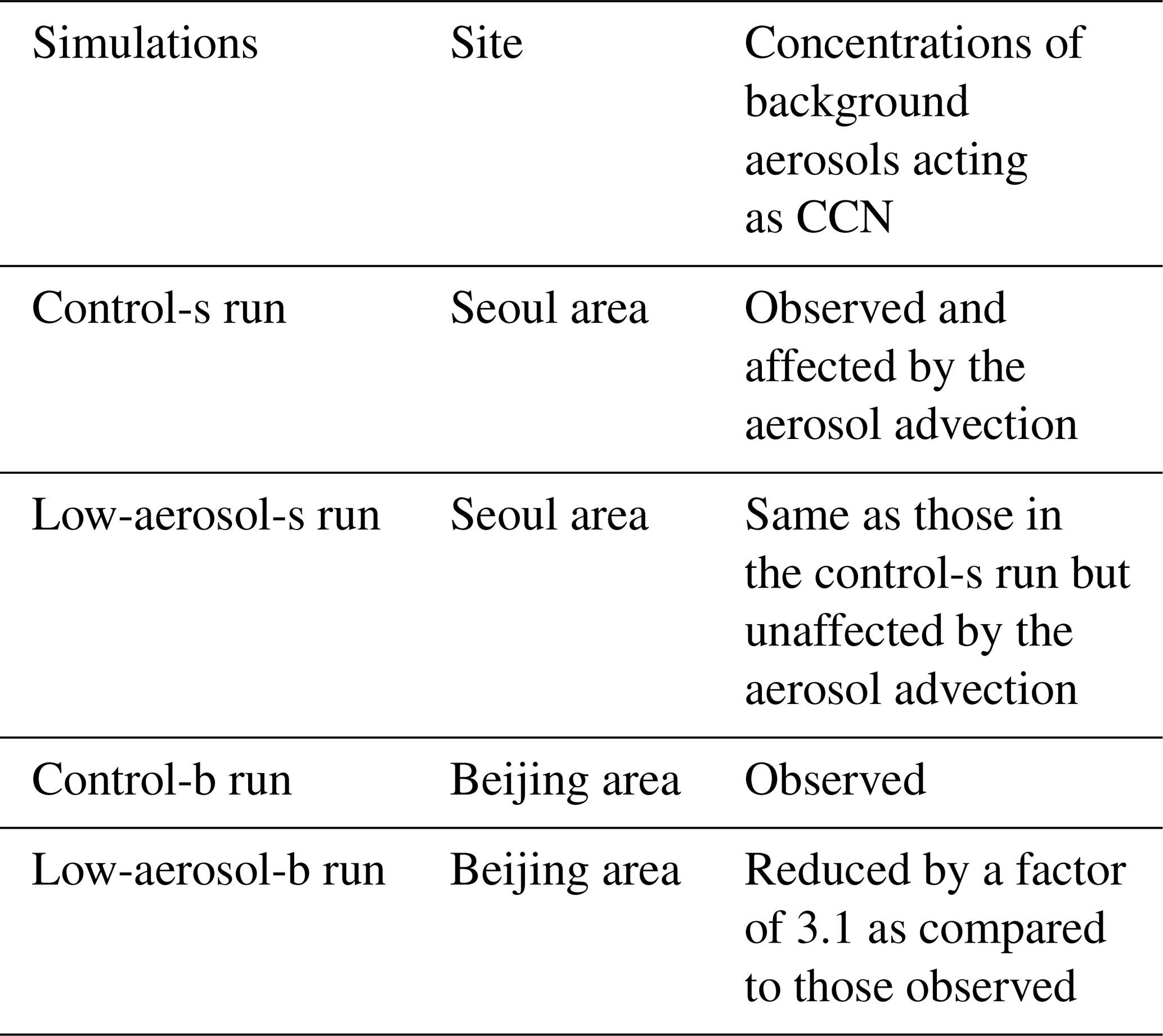
In the low-aerosol-s run, as a way of getting rid of aerosol advection-induced increases in concentrations of aerosols acting as CCN, it is assumed that PM_2.5, which is assumed to represent the mass of aerosols acting as CCN, and the associated background concentration of aerosols acting as CCN after 01:00 LST on 23 December do not evolve with the aerosol advection in the Seoul area. Hence, the background concentration of aerosols acting as CCN at 01:00 LST on 23 December is applied to each time step and grid point at the beginning of the simulation period. However, to isolate CCN effects on clouds, background aerosol concentration acting as INPs at each time step and grid point in the low-aerosol-s run is not different from that in the control-s run during the simulation period. There is reduction in the observed PM_2.5 for the Seoul area by a factor of ∼10 on average over a period between ∼ 07:00 and ∼ 14:00 LST on 24 December, since precipitation scavenges aerosols (Fig. 2). To emulate this scavenging and reflect it in background aerosols acting as CCN for the low-aerosol-s run, PM_2.5 and the corresponding background concentrations of aerosols acting as CCN at each grid point are gradually reduced for the period between 07:00 and 14:00 LST on 24 December. This reduction is done in such a way that background concentrations of aerosols acting as CCN at each grid point at 14:00 LST on 24 December are 10 times lower than that at 07:00 LST on 24 December in the low-aerosol-s run. Then, PM_2.5 and the corresponding background concentrations of aerosols acting as CCN at each grid point at 14:00 LST on 24 December are maintained until the end of the simulation period. This results in the evolution of the average PM_2.5 over the Seoul area in the low-aerosol-s run as shown in Fig. 2. Here, the concentration of background aerosols acting as CCN, which is averaged over the whole domain and simulation period, in the control-s run is 3.1 times higher than that in the low-aerosol-s run. Via comparisons between the runs,it can be examined how the increasing concentration of background aerosols acting as CCN due to the aerosol advection has an impact on clouds. The concentration of background aerosols acting as CCN is different among grid points and time steps in the control-s run. Hence, the ratio of the concentration of background aerosols acting as CCN between the runs is different among grid points and time steps.

For the Beijing case, to examine how aerosols acting as CCN affect clouds and precipitation, we repeat the control-b run with simply reduced concentrations of background aerosols acting as CCN at each time step and grid point by a factor of 3.1. This repeated run is named the low-aerosol-b run. The 3.1-fold increase in aerosol concentrations from the low-aerosol-b run to the control-b is based on the 3.1-fold increase in the average concentration of background aerosols acting as CCN from the low-aerosol-s run to the control-s run. However, as in the control-s and low-aerosol-s runs, to isolate CCN effects on clouds, the background aerosol concentration acting as INPs at each time step and grid point in the low-aerosol-b run is identical to that in the control-b run during the simulation period. Hence, on average, a pair of the control-s and low-aerosol-s runs has the same perturbation of aerosols acting as CCN as in a pair of the control-b and low-aerosol-b runs. Here, we define aerosol perturbation as a relative increase in aerosol concentration when compared to that before the increase occurs. The brief summary of all simulations in this study is given in Table 1.

Table 1 Summary of simulations.

4 Results

4.1 Cumulative precipitation

We compare the observed precipitation to the simulated counterpart in the control-s run for the Seoul case and in the control-b run for the Beijing case. For this comparison, the observed and simulated precipitation rates at the surface are averaged over the domain for each of the Seoul and Beijing cases (Fig. 3a and b). Here, the simulated precipitation rates are smoothed over 1 h. The comparison shows that the evolution of the simulated precipitation rate does not significantly deviate from the observed counterpart (Fig. 3a and b).

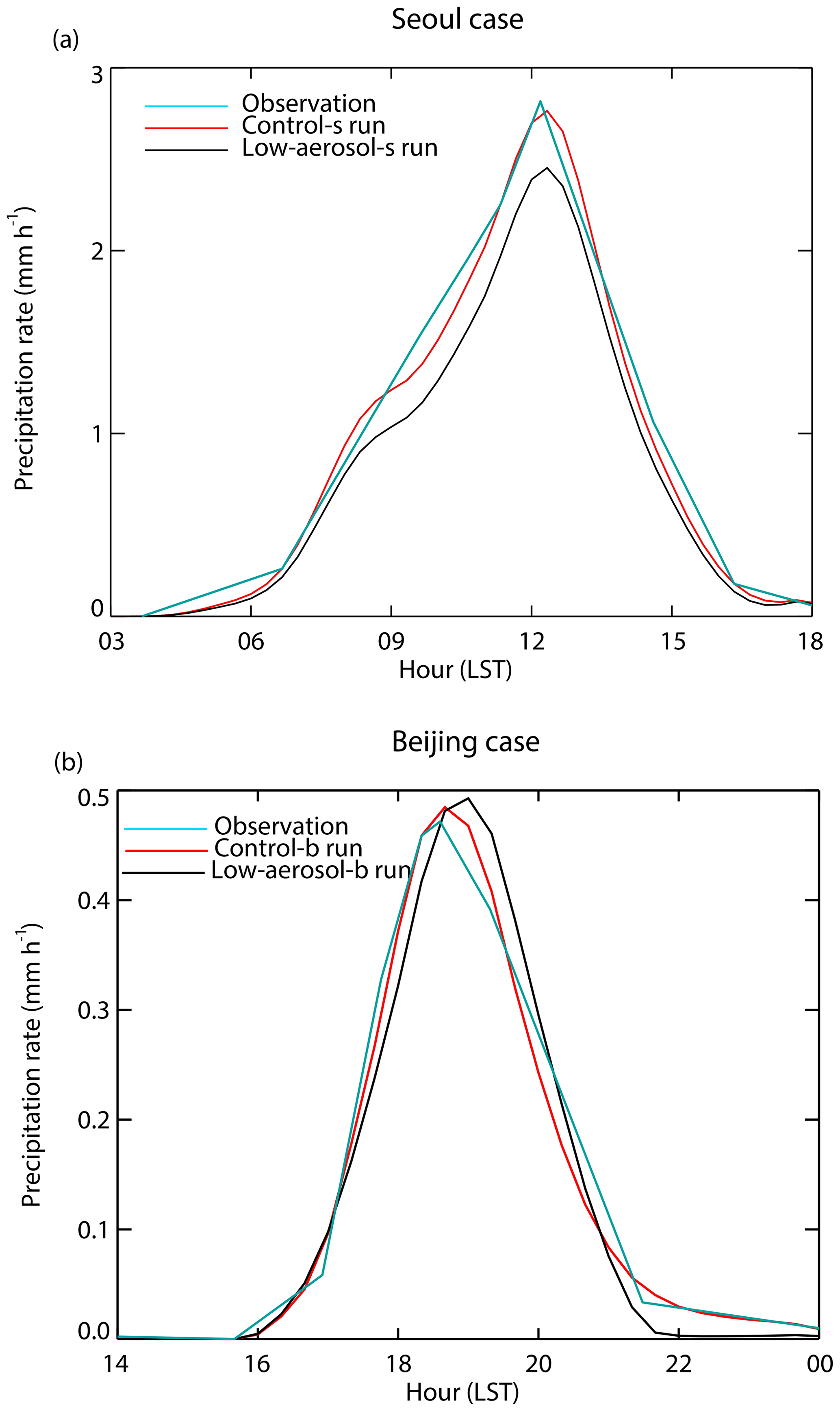
Figure 3 Time series of precipitation rates at the surface, which are averaged over the domain and smoothed over 1 h, (a) for the control-s and low-aerosol-s runs in the Seoul area and (b) for the control-b and low-aerosol-b runs in the Beijing area. In (a) and (b), the averaged and observed precipitation rates over the observation sites in the Seoul and Beijing areas, respectively, are also shown.

In the Seoul case, overall the precipitation rate is higher in the control-s run than in the low-aerosol-s run. As a result of this the domain-averaged cumulative precipitation amount at the last time step is 14.1 and 12.0 mm in the control-s run and the low-aerosol-s run, respectively. The control-s run shows ∼20 % higher cumulative precipitation amount. In the Beijing case, the evolution of the mean precipitation rate in the control-b run is not significantly different from that in the low-aerosol-b run. Due to this, the control-b run shows only ∼2 % higher cumulative precipitation amounts, despite the fact that the concentrations of background aerosols acting as CCN are ∼3 times higher in the control-b run than in the low-aerosol-b run. Note that in the Seoul case, the time-averaged and domain-averaged concentration of background aerosols acting as CCN is also ∼3 times higher in the control-s run than in the low-aerosol-s run. Despite this, the difference in the cumulative precipitation amount between the runs with different concentrations of background aerosols acting as CCN is greater in the Seoul case than in the Beijing case.

4.2 Precipitation, and associated latent-heat and dynamic processes

Figure 4a and b shows the cumulative frequency distributions of precipitation rates at the last time step in the simulations for the Seoul and Beijing cases, respectively. In each of those figures, the observed frequency distribution is shown and compared to the simulated distribution. The observed distribution is obtained by interpolating and extrapolating the observed precipitation rates to grid points and time steps in each of the control-s and control-b runs. The observed maximum precipitation rates are 13.0 and 44.5 mm h⁻¹ for the Seoul and Beijing cases, respectively, and these maximum rates are similar to those in the control-s and control-b runs, respectively. Overall, the observed and simulated frequency distributions are in good agreement for each of the cases. This enables us to assume that results in the control-s (control-b) run are benchmark results to which results in the low-aerosol-s (low-aerosol-b) run can be compared to identify how aerosols acting as CCN have an impact on clouds and precipitation for the Seoul (Beijing) case. Here, it is notable that for the Beijing case, while differences in the cumulative precipitation amount between the control-b and low-aerosol-b runs are not significant, features in the frequency distribution of precipitation rates between those runs are substantially different (Fig. 4b).

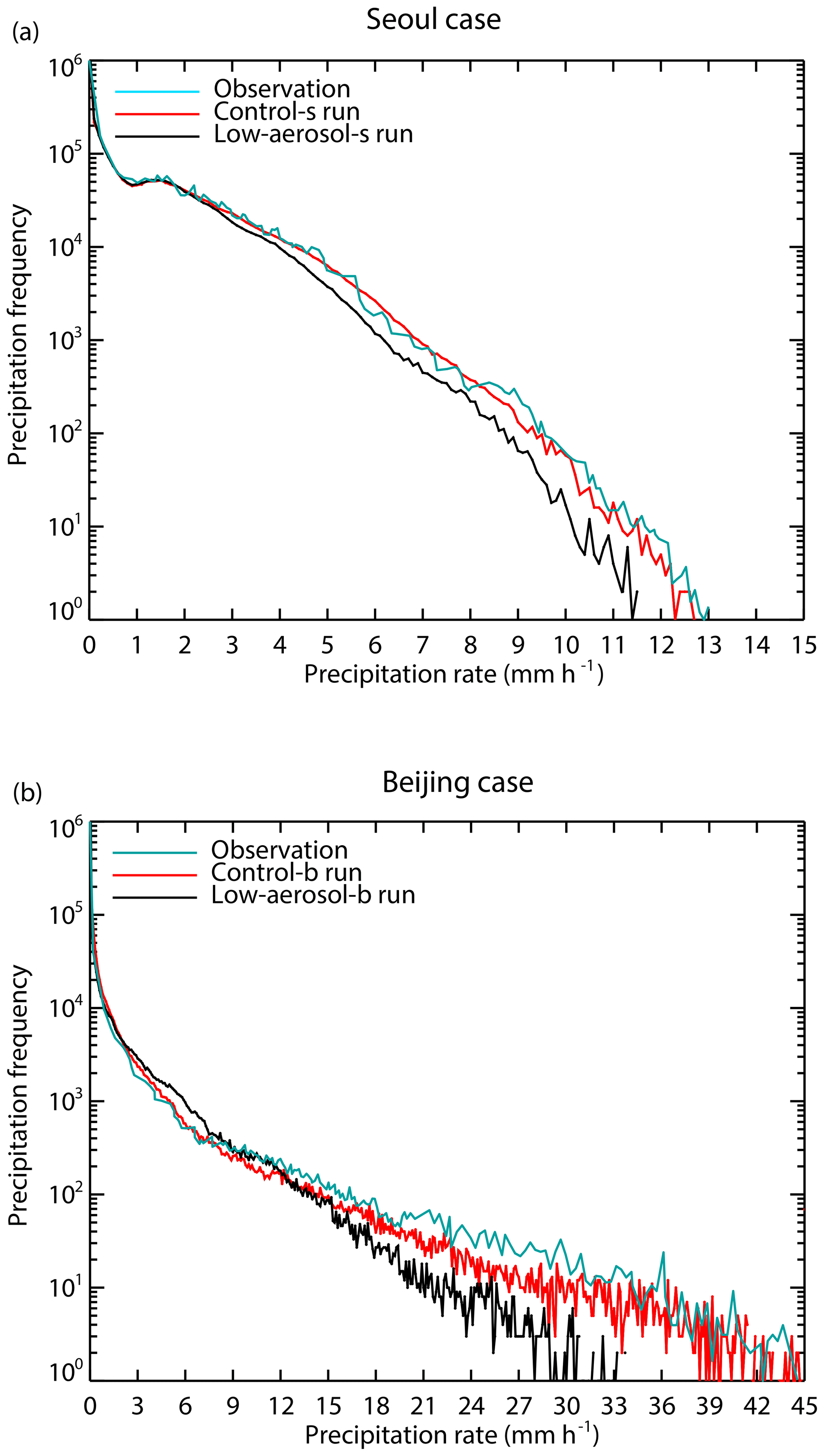
Figure 4 Observed and simulated cumulative frequency distributions of precipitation rates at the surface for (a) the Seoul case, which are collected over the Seoul area, and (b) the Beijing case, which are collected over the Beijing area, at the last time step. Simulated distributions are in the control-s and low-aerosol-s runs for the Seoul case and in the control-b and low-aerosol-b runs for the Beijing case. The observed distribution is obtained by interpolating and extrapolating the observed precipitation rates to grid points and time steps in the control-s and control-b runs for the Seoul and Beijing cases, respectively.

(1) Seoul case

(a) Precipitation frequency distributions

At precipitation rates higher than ∼2 mm h⁻¹, the cumulative precipitation frequency at the last time step is higher in the control-s run as compared to that in the low-aerosol-s run (Fig. 4a). In particular, for the precipitation rate of 11.4 mm h⁻¹, there is an increase in the cumulative frequency by a factor of as much as ∼10 in the control-s run. When it comes to precipitation rates above 11.5 mm h⁻¹, precipitation is present in the control-s run and precipitation is absent in the low-aerosol-s run. At precipitation rates lower than ∼2 mm h⁻¹, differences in the cumulative frequency between the runs are insignificant. Hence, we see that there are significant increases in the frequency of relatively heavy precipitation with rates above ∼2 mm h⁻¹ in the control-s run when compared to that in the low-aerosol-s run. At the last time step, this results in a larger amount of cumulative precipitation in the control-s run than in the low-aerosol-s run.

The time evolution of the cumulative precipitation frequency is shown in Fig. 5. At 06:00 LST on 24 December 2017, which corresponds to the initial stage of the precipitation development, the maximum precipitation rate reaches ∼3 mm h⁻¹ and there is the greater frequency over most of precipitation rates in the control-s run than in the low-aerosol-s run (Fig. 5a). With the time progress from 06:00 to 10:00 LST, the maximum precipitation rate increases to reach 12 mm h⁻¹ and the cumulative frequency is higher over precipitation whose rates are higher than ∼3 mm h⁻¹ in the control-s run, while for precipitation whose rates are lower than ∼3 mm h⁻¹, differences in the cumulative frequency between the runs are negligible (Fig. 5a and b). When time reaches 12:00 LST, which is around time when the peak in the evolution of the area-averaged precipitation rates occurs and thus the system is at its mature stage, the maximum precipitation rate increases up to ∼13 mm h⁻¹ (Figs. 3a and 5c). The basic patterns of differences in the cumulative precipitation frequency between the runs with the maximum precipitation rate around 13 mm h⁻¹, which are established at 12:00 LST, are maintained until the end of the simulation period (Figs. 4a and 5c).

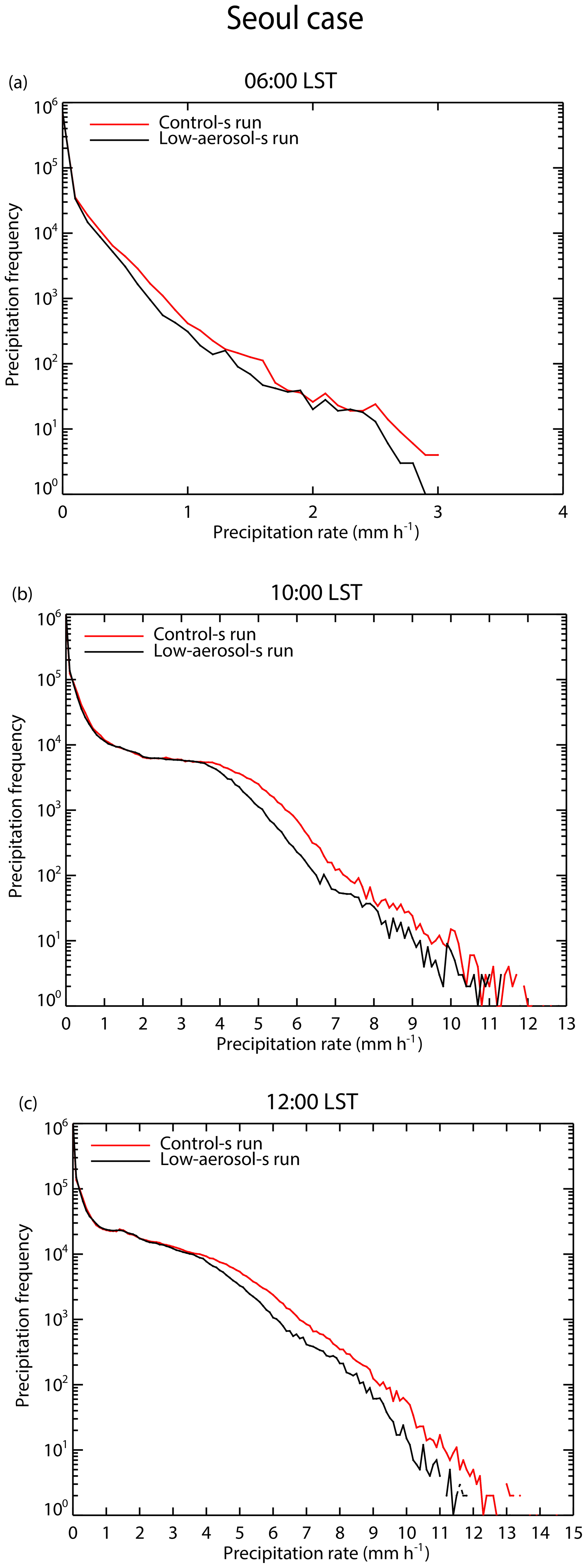
Figure 5 Cumulative frequency distributions of the precipitation rates at the surface in the control-s and low-aerosol-s runs for the Seoul case at (a) 06:00 LST, (b) 10:00 LST and (c) 12:00 LST.

Figure 6 Vertical distributions of differences in the area-averaged condensation, deposition and freezing rates, and cloud-liquid, raindrop, snow and hail mass density, and updraft mass fluxes between the control-s and low-aerosol-s runs at (a) 03:20 LST, (b) 03:40 LST, (c) 06:00 LST and (d) 12:00 LST. The horizontal black line in each panel represents the altitude of freezing or melting. Here, for the sake of the display brevity, snow mass density includes ice-mass density, while hail mass density includes graupel mass density.

(b) Condensation, deposition, updrafts and associated variables

Note that the source of precipitation is precipitable hydrometeors which are raindrops, snow, graupel and hail particles. Droplets and ice crystals are the source of those precipitable hydrometeors mostly via collision and coalescence processes. Droplets and ice crystals gain their mass mostly via condensation and deposition. Based on this, to explain the greater cumulative precipitation amount in the control-s run than in the low-aerosol-s run, the evolutions of differences in condensation, deposition and associated updrafts between the runs are analyzed. The vertical profiles of differences in the area-averaged condensation, deposition and freezing rates, updraft mass fluxes and the associated mass density of each class of hydrometeors between the runs at 03:20, 03:40, 06:00 and 12:00 LST are shown in Fig. 6. In Fig. 6, differences in freezing rates are added for a more comprehensive understanding of processes that are related to differences in cumulative precipitation amounts between the runs. Freezing includes riming processes between liquid and solid hydrometeors and these riming processes act as a source of precipitable hydrometeors. Cloud fractions are 0.32 (0.30), 0.85 (0.82), 0.93 (0.92) and 1.00 (1.00) in the control-s (low-aerosol-s) run at 03:20, 03:40, 06:00 and 12:00 LST, respectively. We see that the cloud fraction varies between 0 % and ∼6 % between the runs. Note that in all of figures, which display snow and hail mass density and include Fig. 6, snow mass density includes ice-crystal mass density, while hail mass density includes graupel mass density for the sake of the display brevity. In Fig. 6, horizontal black lines represent the altitudes of freezing and melting.

Condensation rates in the control-s run start to be larger than that in the low-aerosol-s run at 03:20 LST (Fig. 6a). Higher aerosol or CCN concentrations induce more nucleation of droplets, higher cloud droplet number concentration (CDNC) and associated greater integrated surface of droplets in the control-s run. The CDNC, which is averaged over grid points and time steps with non-zero CDNC, is 1050 and 352 cm⁻³ in the control-s and low-aerosol-s runs, respectively. Hence, more droplet surface is provided for water vapor to condense onto in the control-s run. This leads to more condensation in the control-s run. This establishes stronger feedback between updrafts and condensation, leading to greater droplet (or cloud-liquid) mass at 03:20 LST in the control-s run (Fig. 6a). Then, these stronger feedbacks, which involve stronger updrafts particularly above 2 km in altitude, subsequently induce greater deposition and snow mass as time progresses from 03:20 to 03:40 LST, while more condensation and greater droplet mass are maintained in the control-s run with the time progress to 03:40 LST (Fig. 6b). These stronger updrafts enable clouds to grow higher in the control-s run. This eventually leads to a situation where the maximum cloud depth is ∼7 km in the control-s run and this depth is ∼5 % deeper than that in the low-aerosol-s run for the whole simulation period.

Through aerosol-induced stronger feedbacks between condensation, deposition and updrafts in the control-s run, while more condensation and more overall deposition are maintained in the control-s run, differences in condensation and deposition between the control-s and low-aerosol-s runs increase as time progresses from 03:40 to 06:00 LST (Fig. 6b and c). Associated with this, the greater mass of raindrops and hail particles appears, while the greater mass of droplets and snow in the control-s run than in the low-aerosol-s run is maintained with the time progress from 03:40 to 06:00 LST (Fig. 6c). At 06:00 LST, there is more freezing starting to occur in the control-s run than in the low-aerosol-s run. However, differences in freezing are ∼1 and ∼2 orders of magnitude smaller than those in deposition and condensation, respectively. After 06:00 LST until the time reaches 12:00 LST when the overall differences in the cumulative precipitation frequency between the runs are established, differences in freezing become ∼3 times smaller than those in deposition and ∼1 order of magnitude smaller than those in condensation (Fig. 6c and d). The greater mass of hydrometeors in the control-s run also continues after 06:00 LST until time reaches 12:00 LST (Fig. 6c and d). At 12:00 LST, condensation, deposition and freezing rates are still higher in the control-s run. Here, we see that CCN induced more cumulative precipitation amounts and associated differences in the precipitation frequency distribution between the control-s and low-aerosol-s runs are primarily associated with CCN inducing more condensation, which induce more CCN-induced deposition and higher mass density of hydrometeors as sources of precipitation, but weakly connected to CCN-induced changes in freezing. This is supported by the fact that the time-averaged and domain-averaged differences in freezing rates are ∼1–∼2 order of magnitude smaller than those in condensation and deposition rates.

(c) Condensation frequency distributions and horizontal distributions of condensation and precipitation

Based on the importance of condensation for CCN-induced changes in precipitation, the horizontal distribution of the column-averaged condensation rates over the domain and the cumulative frequency distribution of the column-averaged condensation rates at each time step is obtained. To better visualize the role of condensation in precipitation, the horizontal distribution of the column-averaged condensation rates is superimposed on that of precipitation rates (Fig. 7). At 03:40 LST, condensation mainly occurs around the northern part of the domain as marked by a yellow rectangle. The synoptic wind conditions in the marked area favors the collision between northward and southward winds and the associated convergence around the surface (Fig. 7a and b). This convergence induces updrafts and condensation in the marked area. In the marked area, more aerosols acting as CCN induce more and more extensive condensation, which leads to the higher domain-averaged condensation rates in the control-s run than in the low-aerosol-s run (Figs. 6b and 7a, b). More droplets are formed on more aerosols acting as CCN and more droplets provide more surface areas where condensation occurs and this enables more and more extensive condensation in the control-s run than in the low-aerosol-s run (Figs. 6b and 7a, b).

Figure 7 Spatial distributions of terrain heights, column-averaged condensation rates, surface wind vectors and precipitation rates at (a, b) 03:40 LST, (c, d) 08:40 LST, (e, f) 10:00 LST, and (g, h) 12:00 LST. The distributions in the control-s run are shown in (a, c, e, g), and the distributions in the low-aerosol-s run are shown in (b, d, f, h). Condensation rates are shaded. Dark yellow and dark red contours represent precipitation rates at 0.5 and 3.0 mm h⁻¹, respectively, while beige, light brown and brown contours represent terrain heights at 100, 300 and 600 m, respectively. See text for yellow rectangles in a, b, e, f.

At 06:20 LST, a precipitating system is advected into the domain via the western boundary, and as seen in Fig. 7c and d for 08:40 LST, as time progresses to 08:40 LST, the advected precipitating system is further advected to the east and extended mostly over areas in the northern part of the domain where condensation mainly occurs. This confirms that condensation is the main source of cloud mass and precipitation. In the eastern part of the domain, there are mountains and in particular, higher mountains are on the northeastern part of the domain than in the other parts of the domain. These higher mountains induce forced convection and associated condensation more effectively in the northeastern part than in the other parts. This is in favor of the precipitating system that extends further to the east in the northern part of the domain. Due to more aerosols acting as CCN, condensation, which is induced by forced convection over mountains, is more and more extensive in the control-s run (Fig. 7c and d). In association with this, there is more extension of the precipitating system in the control-s run than in the low-aerosol-s run. This enables the system in the control-s run to reach the eastern boundary at 08:40 LST, which is earlier than in the low-aerosol-s run (Fig. 7c and d). The system in the low-aerosol-s run reaches the eastern boundary at 09:00 LST. Here, we see that although aerosols acting as CCN do not change overall locations of the precipitation system, they affect how fast the system extends to the east by affecting the amount of condensation which is produced by forced convection. Associated with this, as seen in Fig. 8, the control-s run has the much higher cumulative condensation frequency than the low-aerosol-s run over all condensation rates during the period between 07:20 and 09:00 LST. Contributed by this, the higher precipitation frequency over most of the precipitation rates occurs in the control-s run during and after the period (Fig. S1a and b in the Supplement and Fig. 5b and c).

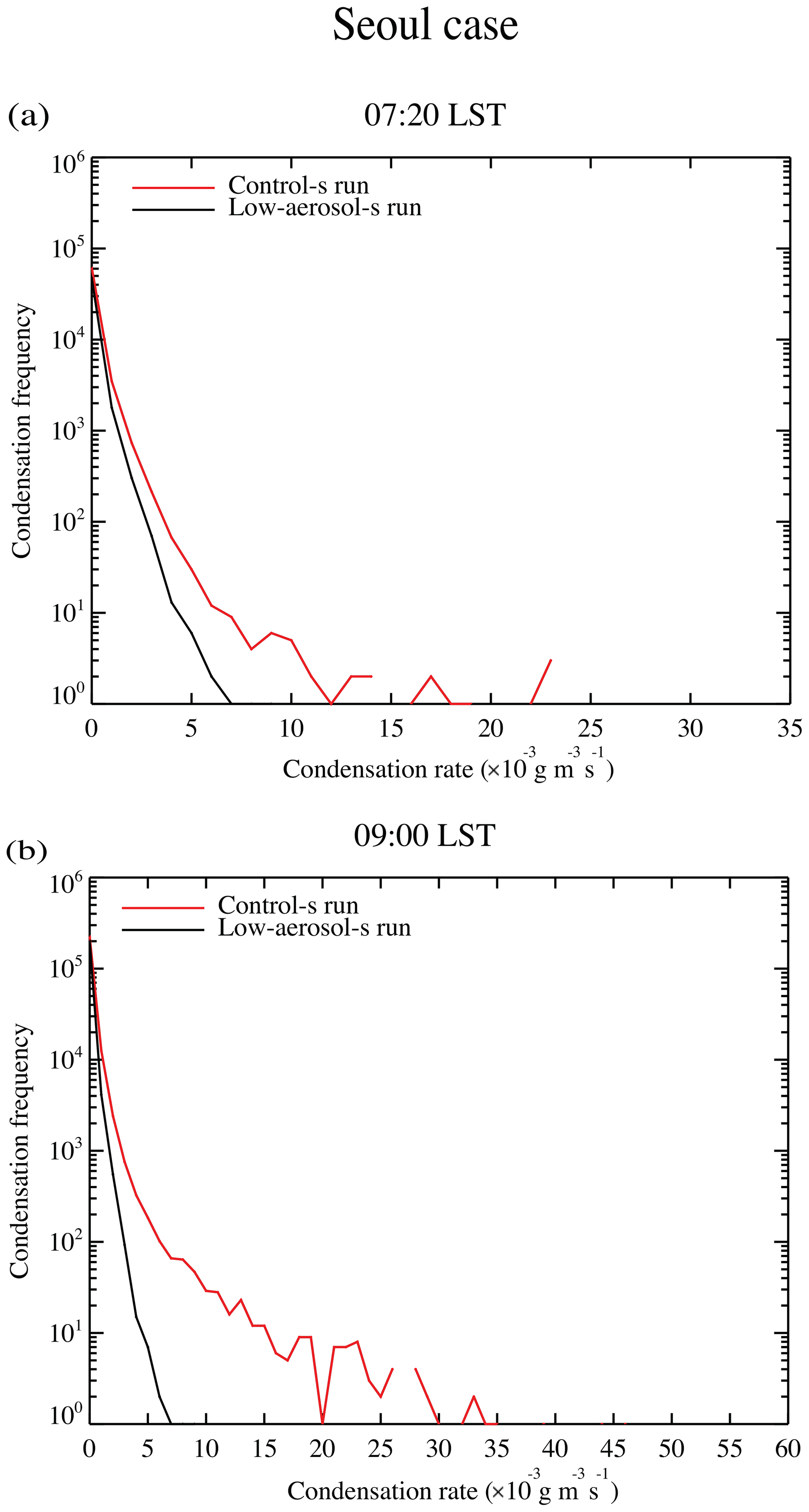
Figure 8 Cumulative frequency distributions of the column-averaged condensation rates in the control-s and low-aerosol-s runs for the Seoul case at (a) 07:20 LST and (b) 09:00 LST.

At 10:00 LST, in the southern part of the domain, there is a precipitating area forming as marked by a yellow rectangle (Fig. 7e and f). The precipitation area in the southern part of the domain extends and merges into the advecting main precipitating system in the northern part of the domain. The merge leads to precipitation that occupies most of the domain at 12:00 LST (Fig. 7g and h). After 10:00 LST, associated with this merge, the maximum precipitation rate increases to 13 mm h⁻¹ at 12:00 LST (Fig. 5c). After 13:00 LST, the precipitation enters its dissipating stage and its area decreases and nearly disappears. Even after the merge, CCN-induced more condensation is maintained and this in turn contributes to a situation where the control-s run has a greater precipitation frequency over most of the precipitation rates than in the low-aerosol-s run until the simulations progress to the last time step (Figs. 4a, 5c and 6d).

(2) Beijing case

Stronger convection and deeper clouds develop in the Beijing case than in the Seoul case. The maximum cloud depth is ∼7 and ∼12 km in the control-s and control-b runs, respectively. In the Seoul case, clouds do not reach the tropopause, while they reach the tropopause in the Beijing case. Deeper clouds in the Beijing case produce the maximum precipitation rate of ∼45 mm h⁻¹ in the control-b run. However, shallow (less deep) clouds in the Seoul case produce the maximum precipitation rate of ∼13 mm h⁻¹ in the control-s run (Fig. 4).

(a) Precipitation frequency distributions

When it comes to precipitation rates higher than ∼12 mm h⁻¹, the control-b run has the higher cumulative precipitation frequency at the last time step than the low-aerosol-b run (Fig. 4b). In particular, for the precipitation rates of 28.1 and 30.0 mm h⁻¹, the cumulative frequency increases by a factor of as much as ∼10. Moreover, regarding precipitation rates higher than ∼33 mm h⁻¹, precipitation is present in the control-b run; however, precipitation is absent in the low-aerosol-b run. Hence, we see that the frequency of comparatively heavy precipitation when it comes to precipitation rates higher than ∼12 mm h⁻¹ rises significantly more in the control-b run as compared to that in the low-aerosol-b run. Below ∼2 mm h⁻¹, there is also the greater precipitation frequency in the control-b run than in the low-aerosol-b run. Unlike the situation for precipitation rates above ∼12 mm h⁻¹ and below ∼2 mm h⁻¹, for precipitation rates from ∼2 to ∼12 mm h⁻¹, the control-aerosol-b run has the lower precipitation frequency than in the low-aerosol-b run. Here, we see that the higher precipitation frequency above ∼12 mm h⁻¹ and below ∼2 mm h⁻¹ balances out the lower precipitation frequency between ∼2 and ∼12 mm h⁻¹ in the control-b run. This results in the similar cumulative precipitation amount between the runs.

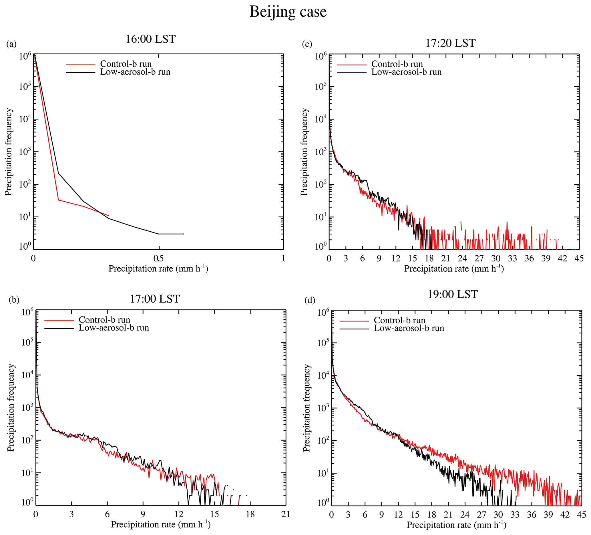
Figure 9 Cumulative frequency distributions of the precipitation rates at the surface in the control-b and low-aerosol-b runs for the Beijing case at (a) 16:00 LST, (b) 17:00 LST, (c) 17:20 LST, and (d) 19:00 LST.

Figure 9 shows the time evolution of the cumulative precipitation frequency. When precipitation starts around 16:00 LST, the higher precipitation frequency occurs over most of precipitation rates in the low-aerosol-run-b run than in the control-b run (Fig. 9a). At 16:00 LST, the maximum precipitation rate is lower than 1.0 mm h⁻¹ for both runs. As time progresses to 17:00 LST, the maximum precipitation rate increases to ∼17 mm h⁻¹ and the higher (lower) cumulative precipitation frequency over precipitation rates higher than ∼12 mm h⁻¹ (between ∼2 and ∼12 mm h⁻¹) in the control-b run than in the low-aerosol-b run, which is described above as shown in Fig. 4b for the last time step, starts to emerge (Fig. 9b). At 17:20 LST, the higher frequency for precipitation rates below 2 mm h⁻¹ in the control-b run, which is also described above as shown in Fig. 4b for the last time step, starts to show up, while the higher (lower) frequency for precipitation rates higher than ∼12 mm h⁻¹ (between ∼2 and ∼12 mm h⁻¹) in the control-b run, which is established at 17:00 LST, is maintained as time progresses from 17:00 to 17:20 LST (Fig. 9c). At 17:20 LST, the maximum precipitation rate increases to 42 (19) mm h⁻¹ in the control-b (low-aerosol-b) run (Fig. 9c). At 19:00 LST, the maximum precipitation rate increases to ∼45 (33) mm h⁻¹ for the control-b (low-aerosol-b) run, while the qualitative nature of differences in the precipitation frequency distributions with the tipping precipitation rates of ∼2 and ∼12 mm h⁻¹ between the runs does not vary much between 17:20 and 19:00 LST (Fig. 9c and d). The qualitative nature of differences in the cumulative precipitation frequency between the runs and the maximum precipitation rates in each of the runs, which are established at 19:00 LST, do not vary significantly until the end of the simulation period (Figs. 4b and 9d).

Figure 10 Same as Fig. 6 but for differences between the control-b and low-aerosol-b runs at (a) 14:20 LST, (b) 15:40 LST, (c) 16:00 LST, (d) 17:20 LST and (e) 19:00 LST.

(b) Condensation, deposition, updrafts and associated variables

As done for the Seoul case, as a way of better understanding differences in the cumulative precipitation amount and frequency between the control-b and low-aerosol-b runs, the evolution of differences in the vertical distributions of the area-averaged condensation rates, deposition rates, freezing rates, the mass density of each class of hydrometeors and updrafts mass fluxes are obtained and shown in Fig. 10. Cloud fractions are 0.12 (0.11), 0.25 (0.22), 0.36 (0.32), 0.43 (0.40) and 0.48 (0.47) in the control-b (low-aerosol-b) run at 14:20, 15:40, 16:00, 17:20 and 19:00 LST, respectively. Here, we see that cloud fraction varies by ∼2 %–12 % between the runs. In Fig. 10, horizontal black lines represent the altitudes of freezing and melting. As seen in Fig. 3b, precipitation starts around 16:00 LST but differences in condensation rates start at 14:20 LST with higher condensation rates in the control-b run (Fig. 10a). Similar to the situation in the Seoul case, higher concentrations of aerosols acting as CCN induce more nucleation of droplets, higher CDNC and associated greater integrated surface of droplets in the control-b run. The CDNC, which is averaged over grid points and time steps with non-zero CDNC, is 992 and 341 cm⁻³ in the control-b and low-aerosol-b runs, respectively. Hence, more droplet surface is provided for water vapor to condense onto in the control-b run. This leads to more condensation in the control-b run. Due to this, cloud-liquid or droplet mass becomes greater in the control-b run at 14:20 LST (Fig. 10a). Increased condensation rates induce increased condensational heating and thus intensified updrafts (Fig. 10a). These updrafts enable the maximum cloud depth to be ∼12 km in the control-b run and this depth is just ∼1 % deeper than that in the low-aerosol-b run for the whole simulation period. This negligible difference in the maximum cloud depth between the runs is due to the fact that clouds with the maximum depth reach the tropopause in both runs and thus there is not much wiggle room to make significant differences in cloud depth between the runs.

When the time reaches 15:40 LST, deposition rates and snow mass start to show differences between the runs, while higher condensation rates and droplet mass are maintained in the control-b run with the time progress from 14:20 to 15:40 LST. However, unlike the situation in the Seoul case, higher concentrations of aerosols acting as CCN result in lower deposition rates and snow mass in the control-b run (Fig. 10b). When time progresses from 15:40 to 16:00 LST, differences in freezing start to occur and freezing rates are lower (higher) at altitudes between ∼6 and ∼8 km (∼4 and ∼6 km), while higher condensation rates and droplet mass, and lower snow mass are maintained in the control-b run (Fig. 10c). Due to stronger updrafts, which are mainly ascribed to more condensation, deposition rates start to be higher at altitudes between ∼7 and ∼9 km and freezing rates are higher at altitudes between ∼4 and ∼6 km in the control-b run with the time progress from 15:40 to 16:00 LST (Fig. 10c). Differences in freezing rates are similar to those in deposition and ∼2 orders of magnitude smaller than those in condensation at 16:00 LST (Fig. 10c). At 16:00 LST, differences in hail mass between the runs emerge and hail mass is slightly lower in the control-b run (Fig. 10c). At 17:20 LST, overall, freezing rates are lower at altitudes between ∼4 and ∼8 km, while overall the snow and hail mass is still lower, and droplet mass is still higher in the control-b run (Fig. 10d). Differences in freezing rates are ∼2 times smaller than those in deposition and ∼1 order of magnitude smaller than those in condensation at 17:20 LST (Fig. 10d). Due to more condensation and droplet mass, greater raindrop mass starts to emerge in the control-b run at 17:20 LST (Fig. 10d). As the time progresses to 19:00 LST, deposition rates become lower at the altitudes from ∼7 to ∼12 km and overall freezing rates become higher at altitudes from ∼4 to ∼10 km in the control-b run (Fig. 10e). Overall, lower snow and hail mass maintains in the control-b run as time progresses from 17:20 to 19:00 LST. As time progresses from 17:20 to 19:00 LST, overall higher condensation rates, droplet and raindrop mass are maintained in the control-b run (Fig. 10e). Here, while the time-averaged and domain-averaged deposition (condensation and freezing) rates are lower (higher) in the control-b run over the whole simulation period, the average differences in freezing rates are ∼1 –∼2 orders of magnitude smaller than those in deposition and condensation rates between the runs. Hence, more condensation (but not deposition and freezing) is a main cause of stronger updrafts in the control-b run. More condensation and more freezing tend to induce increases in the mass of precipitable hydrometeors in the control-b run. Less deposition tends to induce decreases in the mass of precipitable hydrometeors in the control-b run. This competition between condensation, deposition and freezing leads to negligible differences in the cumulative precipitation amount at the last time step between the control-b and low-aerosol-b runs, although roles of freezing in this competition are negligible compared to those of condensation and deposition.

(c) Condensation frequency distributions, horizontal distributions of condensation and precipitation, and condensation-precipitation correlations

Figure 11 shows the horizontal distribution of the column-averaged condensation rates over the domain and Fig. 12 shows the cumulative frequency distributions of column-averaged condensation rates at selected times. As in the Seoul case, the horizontal distribution of condensation rates is superimposed on that of precipitation rates and the terrain in Fig. 11. At 14:20 LST, condensation starts to occur in places with mountains, which induce forced convection, and condensation is concentrated around the center of the domain as marked by a yellow circle (Fig. 11a and b). Note that condensation does not occur in the plain area which is the south of the 100 m terrain height contour line (Fig. 11a and b). Due to higher concentrations of aerosols acting as CCN, there is more condensation around the center in the control-b run than in the low-aerosol-b run (Fig. 11a and b). This leads to a situation where the control-b run has higher area-averaged condensation rates than the low-aerosol-b run (Fig. 10a). Then, as time progresses to 17:20 LST, the condensation area extends to the eastern and western parts of the domain mostly over mountain areas (Fig. 11c and d). Hence, the main source of condensation is considered to be forced convection over mountains. As seen in Fig. 11c and d, higher concentrations of aerosols acting as CCN induce the control-b run to have much more condensation spots and thus much bigger areas with condensation than the low-aerosol-b run at 17:20 LST. Associated with this, CCN-induced more condensation in the control-b run is maintained with the time progress to 17:20 LST (Fig. 10d). At 17:20 LST, precipitation mainly occurs in a spot which is in the western part of areas with relatively high condensation rates (Fig. 11c and d).

Figure 11 Spatial distributions of terrain heights, column-averaged condensation rates, surface wind vectors and precipitation rates at (a, b) 14:20 LST, and (c, d) 17:20 LST. (a, c) are for the control-b run and (b, d) are for the low-aerosol-b run. Condensation rates are shaded. Dark yellow and dark red contours represent precipitation rates at 1.0 and 2.0 mm h⁻¹, respectively, while beige, light brown, brown and dark brown contours represent terrain heights at 100, 500, 1000 and 1500 m, respectively. See text for yellow circles in (a) and (b).

Figure 12 Cumulative frequency distributions of the column-averaged condensation rates in the control-b and low-aerosol-b runs for the Beijing case at (a) 17:20 LST and (b) 19:00 LST.

At 17:20 LST, as seen in the cumulative frequency of condensation rates, the control-b run has the higher condensation frequency above a condensation rate of $\sim \mathrm{10}\times {\mathrm{10}}^{-\mathrm{3}}$ g m⁻³ s⁻¹ and below that of $\sim \mathrm{3}\times {\mathrm{10}}^{-\mathrm{3}}$ g m⁻³ s⁻¹ than the low-aerosol-b run (Fig. 12a). This pattern of differences in the condensation frequency distribution with the tipping condensation rate points at $\sim \mathrm{10}\times {\mathrm{10}}^{-\mathrm{3}}$ and $\sim \mathrm{3}\times {\mathrm{10}}^{-\mathrm{3}}$ g m⁻² s⁻¹ continues up to 19:00 LST (Fig. 12b). Figure 13 shows the mean precipitation rate over each of the column-averaged condensation rates for the period up to 17:20 LST in the control-b run. A column-averaged condensation rate in an air column with a precipitation rate at its surface is obtained and these condensation and precipitation rates are paired at each column and time step. Then, collected precipitation rates are classified and grouped based on the corresponding paired column-averaged condensation rates. The classified precipitation rates corresponding to each of the column-averaged condensation rates are averaged arithmetically to construct Fig. 13. There are only less than 10 % differences in the mean precipitation rate for each of the column-averaged condensation rates between the control-b and low-aerosol-b runs (not shown). Figure 13 shows that generally a higher condensation rate is related to a higher mean precipitation rate. It is also roughly shown that, according to the mean precipitation rate for each condensation rate, overall, condensation rates below $\sim \mathrm{3}\times {\mathrm{10}}^{-\mathrm{3}}$ g m⁻³ s⁻¹ and above $\sim \mathrm{10}\times {\mathrm{10}}^{-\mathrm{3}}$ g m⁻³ s⁻¹ are correlated with precipitation rates below ∼2 mm h⁻¹ and above ∼12 mm h⁻¹, respectively, while condensation rates between ∼3 and $\sim \mathrm{10}\times {\mathrm{10}}^{-\mathrm{3}}$ g m⁻³ s⁻¹ are correlated with precipitation rates between ∼2 and ∼12 mm h⁻¹ (Fig. 13). Hence, on average, the higher frequency of condensation with rates above $\sim \mathrm{10}\times {\mathrm{10}}^{-\mathrm{3}}$ g m⁻³ s⁻¹ and below $\sim \mathrm{3}\times {\mathrm{10}}^{-\mathrm{3}}$ g m⁻³ s⁻¹ can be considered to lead to the higher frequency of precipitation with rates higher than ∼12 mm h⁻¹ and lower than ∼2 mm h⁻¹ in the control-b run, respectively. It can also be considered that the lower condensation frequency between ∼3 and $\sim \mathrm{10}\times {\mathrm{10}}^{-\mathrm{3}}$ g m⁻³ s⁻¹ leads to the lower precipitation frequency between ∼2 and ∼12 mm h⁻¹ in the control-b run. It is found that this correspondence between condensation and precipitation rates is also valid if analyses to construct Fig. 13 are repeated only for a time point at 16:30 LST or for a period between 16:30 and 17:00 LST. This time point and period is related to analyses of the moist static energy as described in Sect. e.

At 17:20 LST, the larger precipitation frequency between ∼2 and ∼12 mm h⁻¹ in the low-aerosol-b run nearly offsets the larger precipitation frequency in the other ranges of precipitation rates in the control-b run (Fig. 9c). This leads to the similar average precipitation rates between the runs at 17:20 LST and contributes to the similar cumulative precipitation at the last time step between the runs (Fig. 3b).

(d) Evaporation and gust fronts

As time progresses from 17:00 to 19:00 LST, the precipitation system moves northward (Fig. 14). At the core of the precipitation system there is the formation of horizontal outflow at 17:00 LST due to evaporation and downdrafts(Fig. 14a and b). The core is represented by the field of precipitation with rates higher than 1 mm h⁻¹ in Fig. 14. At the core, the northward outflow is magnified by the northward synoptic scale wind and the outflow in the other directions is offset by the northward wind. Hence, the outflow is mainly northward from 17:00 LST onwards as marked by yellow circles in Fig. 14. This enables convergence or a gust front, which is produced by the outflow from the core, to be mainly formed at the north of the core. Note that the intensity of a gust front is proportional to that of the outflow from a core of precipitation or convective system (Weisman and Klemp, 1982; Houze, 1993). The strong gust front at the north of the core generates strong updrafts, a significant amount of condensation and precipitation. Then, a subsequent area with clouds and precipitation is formed at the north of the core as time progresses, which means that the precipitation system extends or moves to the north as seen in comparisons between subpanels with different times in Fig. 14. This movement, which is induced by collaborative work between outflow, synoptic wind and gust fronts, is typical in deep convective clouds.

Figure 13 Mean precipitation rates corresponding to each column-averaged condensation rate for the period between 14:00 and 17:20 LST in the control-b run. One standard deviation of precipitation rates is represented by a vertical bar at each condensation rate.

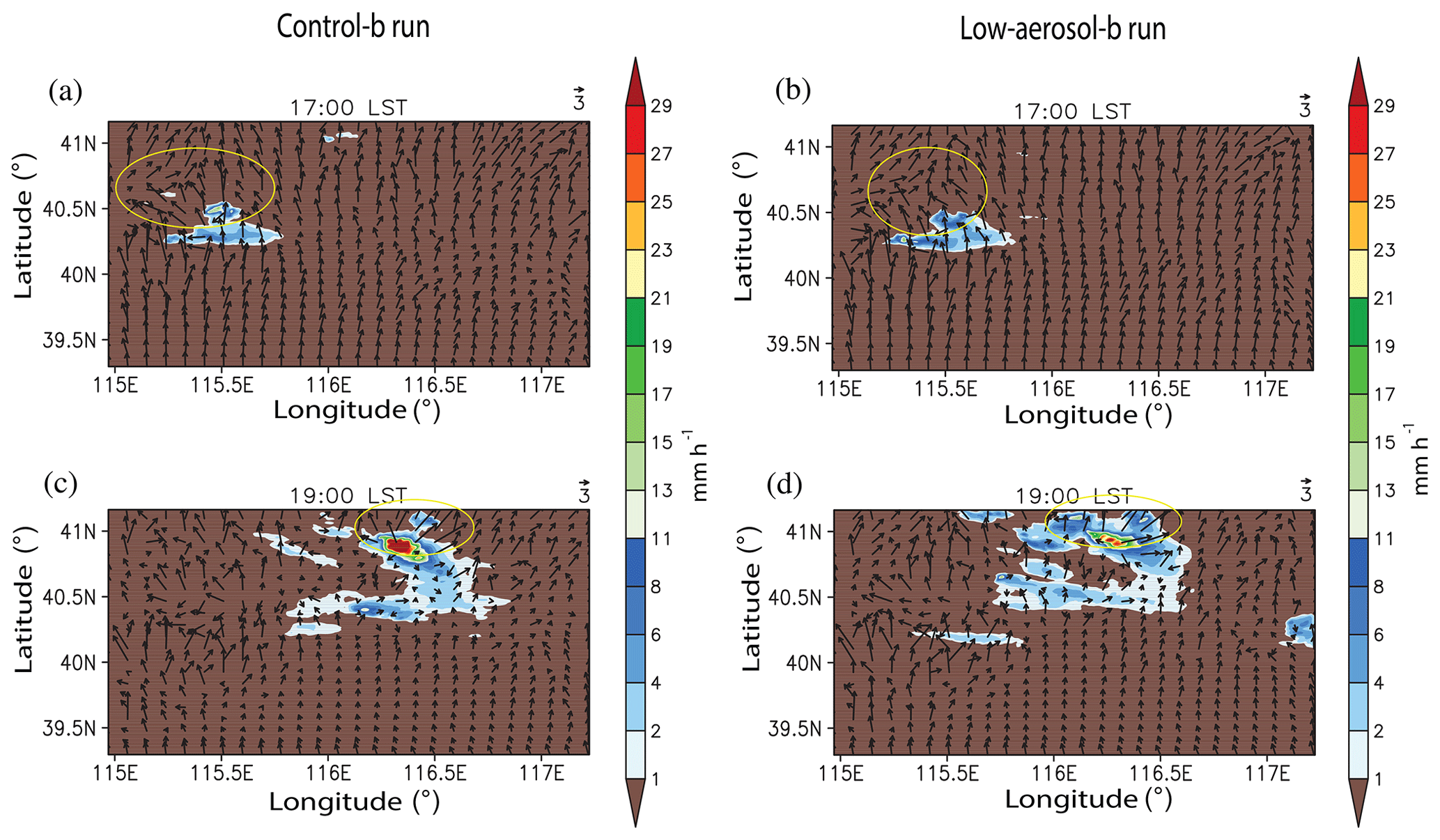
Figure 14 Spatial distributions of precipitation rates (shaded) and wind vectors (arrows) for the Beijing case at (a, b) 17:00 LST, and (c, d) 19:00 LST. The distributions in the control-b run are in (a, c). The distributions in the low-aerosol-b run are in (b, d).

As described above, more droplet nucleation and greater integrated droplet surface induce more condensation before 17:00 LST in the control-b run. This and the lower efficiency of collision and collection among droplets enable the control-b run to have a larger amount of cloud liquid or droplets as a source of evaporation. This in turn enables more droplet evaporation, more associated cooling and stronger downdrafts, although there is less rain evaporation in the control-b run, particularly for the period from 17:00 to 19:00 LST. The time-averaged and domain-averaged droplet and rain evaporation rates are 0.72 (0.31) and 0.08 (0.13) g m⁻³ h⁻¹, respectively, while the time-averaged and domain-averaged downdraft mass flux is 0.15 (0.10) kg m⁻² s⁻¹ over the period from 17:00 to 19:00 LST in the control-b (low-aerosol-b) run. More evaporation of droplets and associated stronger downdrafts with higher concentrations of aerosols acting as CCN have been shown by numerous previous studies (e.g., Tao, 2007; Tao et al., 2012; Khain et al., 2008; Lee et al., 2018).

During the period between 17:00 and 19:00 LST, with the development of convergence or the gust front, as mentioned above, the maximum precipitation rate increases from ∼17 (17) to ∼45 (33) mm h⁻¹ in the control-b (low-aerosol-b) run (Fig. 9). This indicates that the gust-front development contributes to the overall intensification of the precipitation system, while it moves northward. If there was only northward synoptic-scale wind with no formation of the gust front, the system would move northward with less intensification. Over the period from 17:00 to 19:00 LST, stronger downdrafts and associated stronger outflow generate a stronger gust front and more subsequent condensation in the control-b run. This substantially enhances the small initial difference, which is at 17:00 LST, in the frequency of precipitation with rates above ∼12 mm h⁻¹ between the runs as time progresses from 17:00 to 19:00 LST (Fig. 9). Associated with this, as time progresses the nearly identical maximum precipitation rate between the runs at 17:00 LST turns into a significantly higher maximum precipitation rate in the control-b run than in the low-aerosol-b run (Fig. 9). Around 19:00 LST, the system enters its dissipating stage, accompanied by reduction in the precipitating area and the area-averaged precipitation rate (Fig. 3b).

(e) Moist static energy

Condensation, which controls droplet mass and precipitation, is controlled by updrafts, which in turn are controlled by instability. One of the important factors that maintain instability is the moist static energy. Motivated by this, to better understand differences in the precipitation frequency distribution in association with those in the condensation frequency distribution between the control-b and low-aerosol-b runs, we calculate the flux of the moist static energy and the flux is defined as

$$\begin{array}{}\text{(1)}& \mathrm{Fs}=S\times \mathit{\rho }\times \mathit{V},\end{array}$$

where Fs represents the flux of the moist static energy, S the moist static energy, ρ the air density and V the horizontal wind vector. In Eq. (1), we see that the flux is in the vector form and has two components, which are its magnitude and direction. The fluxes of the moist static energy in the PBL are obtained over the domain at 16:30 LST, since in general, the moist static energy in the PBL has much stronger effects on instability and updrafts than that above the PBL. In particular, we focus on the PBL fluxes of the energy that cross the boundary over a time step at 16:30 LST between areas with the column-averaged condensation rate from $\mathrm{3}\times {\mathrm{10}}^{-\mathrm{3}}$ to $\mathrm{10}\times {\mathrm{10}}^{-\mathrm{3}}$ g m⁻³ s⁻¹, which are referred to as `area A, and those with the column-averaged condensation rate above $\mathrm{10}\times {\mathrm{10}}^{-\mathrm{3}}$ g m⁻³ s⁻¹, which are referred to as area B. This is because we are interested in the exchange of the moist static energy between areas A and B and this exchange can be seen by looking at those fluxes which cross the boundary between those areas.

We are interested in the exchange of the energy. This is because we hypothesized that the exchange somehow alters instability in each of areas A and B in a way that there are increases (decreases) in instability, the updraft intensity, condensation and precipitation with increasing concentrations of aerosols acting as CCN in area B (A). This hypothesis leads to the higher (lower) frequency of condensation with rates higher than $\mathrm{10}\times {\mathrm{10}}^{-\mathrm{3}}$ g m⁻³ s⁻¹ (between $\mathrm{3}\times {\mathrm{10}}^{-\mathrm{3}}$ and $\mathrm{10}\times {\mathrm{10}}^{-\mathrm{3}}$ g m⁻³ s⁻¹) and precipitation with rates higher than 12 mm h⁻¹ (between 2 and 12 mm h⁻¹) in the control-b run than in the low-aerosol-b run. When the PBL fluxes which cross the boundary over the time step at 16:30 LST are summed at 16:30 LST, there is the net flux from area A to area B. This means that there is a net transportation of the moist static energy from areas with condensation rates between $\mathrm{3}\times {\mathrm{10}}^{-\mathrm{3}}$ and $\mathrm{10}\times {\mathrm{10}}^{-\mathrm{3}}$ g m⁻³ s⁻¹ to those with condensation rates greater than $\mathrm{10}\times {\mathrm{10}}^{-\mathrm{3}}$ g m⁻³ s⁻¹ in the PBL at 16:30 LST as shown in Table 2. Table 2 shows the net summed flux of the moist static energy which crosses the boundary between areas A and B in the control-b run as well as the low-aerosol-b run. To calculate the net flux at 16:30 LST in Table 2, the fluxes which cross the boundary between areas A and B over the time step at 16:30 LST only at grid points in the PBL are summed. For the calculation, the flux from area A to area B has a positive sign, while the flux from area B to area A has a negative sign. Since the net flux is positive for both of the runs as shown in Table 2, there is the net flux from area A to area B in the PBL. The above-described analysis for the fluxes crossing the boundary between areas A and B is repeated for every time step between 16:30 and 17:00 LST and based on this, the net summed flux over the period between 16:30 and 17:00 LST is obtained. As shown in Table 2, the net flux for the period between 16:30 and 17:00 LST is also positive as in the situation only for 16:30 LST. This means that there is the net transportation of the moist static energy from area A to area B in the PBL during the period between 16:30 and 17:00 LST.

Table 2 The net flux of the moist static energy which crosses the boundary between areas A and B at 16:30 LST and for a period from 16:30 to 17:00 LST.

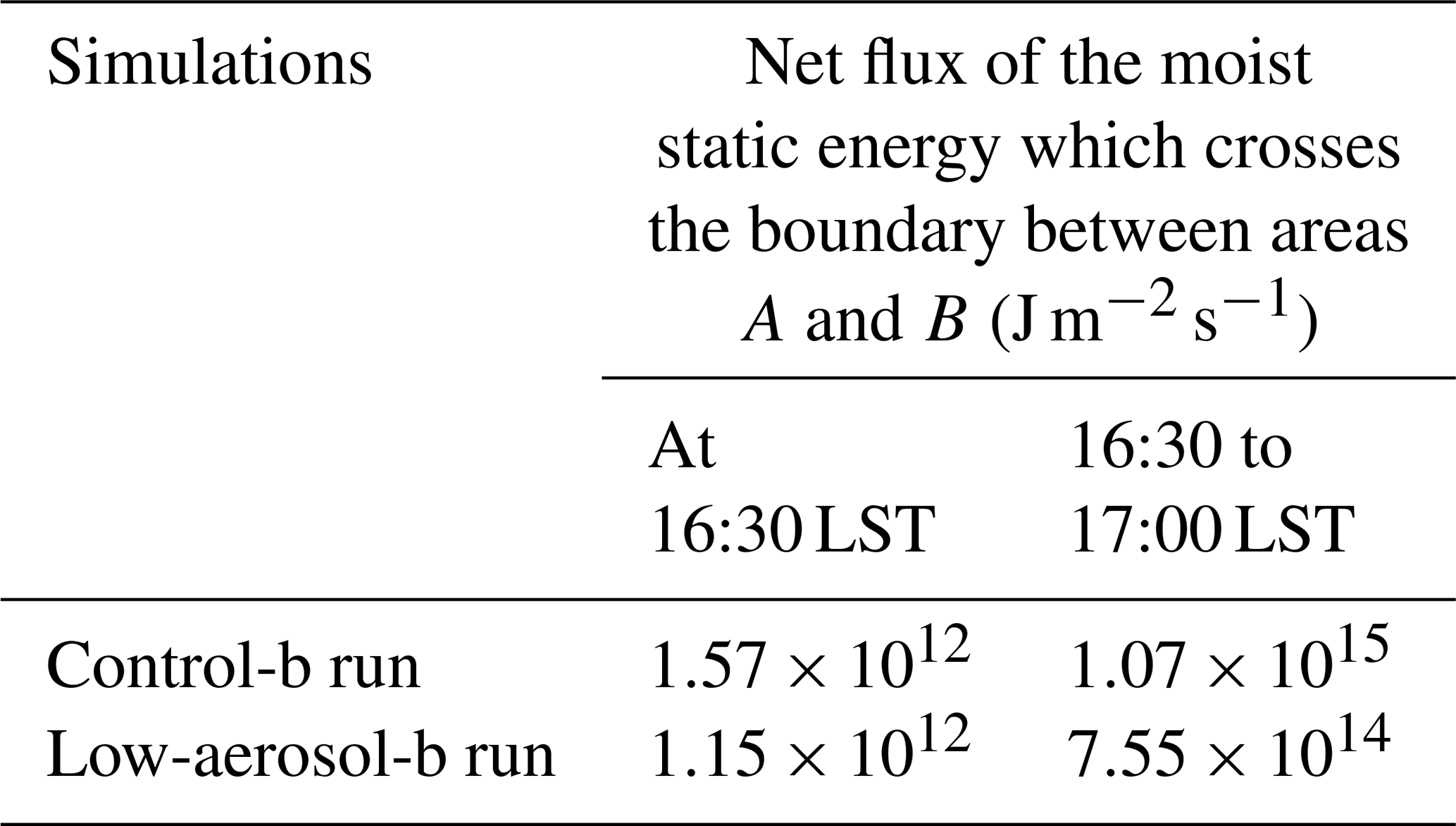
At 16:30 LST, condensation with rates above $\mathrm{10}\times {\mathrm{10}}^{-\mathrm{3}}$ g m⁻³ s⁻¹ starts to develop and this forms area B. Area B has stronger updrafts via greater condensational heating than in other areas, including area A, with lower condensation rates. Stronger updrafts in area B induce the convergence of air and associated moist static energy from area A to area B. Since the average condensation rate and updrafts at 16:30 LST over area B are higher and stronger due to increasing concentrations of aerosols acting as CCN, the air convergence and the associated transportation of the moist static energy in the PBL from area A to area B are stronger and more in the control-b run than in the low-aerosol-b run (Table 2). Stated differently, area B steals the moist static energy from area A, and this occurs more effectively in the control-b run. This increases instability and further intensifies updrafts in area B, and decreases instability and weakens updrafts in area A, while these increases and decreases (intensification and weakening) of instability (updrafts) are greater in the control-b run for the period from 16:30 to 17:00 LST. This increases condensation, cloud mass and precipitation with rates higher than 12 mm h⁻¹ in area B, and decreases condensation, cloud mass and precipitation with rates from 2 to 12 mm h⁻¹ in area A. These increases and decreases occur more effectively for the control-b run than for the low-aerosol-b run during the period. This in turn leads to the lower precipitation frequency for the precipitation rates from 2 to 12 mm h⁻¹ and the higher frequency for the precipitation with rates higher than 12 mm h⁻¹ at 17:00 LST in the control-b run (Fig. 9b). The weakened updrafts and reduced condensation turn a portion of precipitation with rates between 2 and 12 mm h⁻¹ to precipitation with rates below 2 mm h⁻¹, and this takes place more efficiently in the control-b run during the period between 16:30 and 17:00 LST. This eventually increases the frequency of precipitation rates below 2 mm h⁻¹ and this increase is greater for the control-b run, leading to the greater precipitation frequency for the precipitation rates below 2 mm h⁻¹ in the control-b run at 17:20 LST (Fig. 9c).

5 Discussion

Comparison of the Seoul and Beijing cases

In this section, we compare the Seoul case to the Beijing case. For the comparison, remember that on average a pair of the control-s and low-aerosol-s runs has the same perturbation of aerosols acting as CCN as in a pair of the control-b and low-aerosol-b runs. Associated with the fact that clouds in the Seoul case are less deep than those in the Beijing case, overall updrafts in the Seoul case are not as strong as those in the Beijing case. Hence, unlike the situation in the Beijing case, stronger updrafts, which accompany higher condensation rates, and associated convergence in the Seoul case are not strong enough to steal a sufficient amount of the moist static energy from weaker updrafts which accompany lower condensation rates. This makes the redistribution of the moist static energy between areas with relatively higher condensation rates and those with relatively lower condensation rates, such as that between areas A and B for the Beijing case, ineffective for the Seoul case. Due to this, the sign of CCN-induced changes in the frequency of precipitation rates does not vary throughout all of the precipitation rates except for the range of low precipitation rates where there are nearly no CCN-induced changes in the frequency in the Seoul case as shown in Fig. 4a. As seen in Fig. 4a, mainly due to increases in condensation and deposition, precipitation frequency increases for most precipitation rates, although the precipitation frequency does not show significant changes as the concentration of aerosols acting as CCN increases for relatively low precipitation rates in the control-s run as compared to the low-aerosol-s run. This means that there are no tipping precipitation rates where the sign of CCN-induced changes in the frequency of precipitation rates changes in the Seoul case, contributing to the higher cumulative precipitation amount in the simulation with higher concentrations of aerosols acting as CCN for the Seoul case, which are different from the situation in the Beijing case.

In the Beijing case with deeper clouds as compared to those in the Seoul case, clouds develop gust fronts via strong downdrafts and associated strong outflow. These gust fronts play an important role in developing strong convection and associated high precipitation rates. Unlike the situation in the Seoul case, there are strong clouds and associated updraft entities that are able to steal heat and moisture (or the moist static energy) as sources of instability from areas with relatively less strong clouds and updrafts with medium strength; note that these strong clouds here involve stronger updrafts via greater condensational heating as described in Section e above and this enables these clouds to be thicker and have higher cloud mass than these less strong clouds. This further intensifies strong clouds and weakens less strong clouds with medium strength. Due to this, the cumulative frequency of heavy (medium) precipitation in association with strong clouds (less strong clouds with medium strength) increases (decreases). Some of the weakened clouds eventually produce light precipitation, which increase the cumulative frequency for light precipitation. The intensification of strong clouds and the weakening of less strong clouds with medium strength gets more effective with increasing concentration of aerosols acting as CCN. Hence, in the Beijing case, for medium precipitation in association with less strong clouds, the simulation with higher concentration of aerosols acting as CCN shows the lower cumulative precipitation frequency at the last time step. However, for heavy and light precipitation, the simulation with higher concentrations of aerosols acting as CCN shows the higher cumulative precipitation frequency at the last time step; remember that heavy precipitation is associated with strong clouds. These differential responses of precipitation to increasing concentration of aerosols acting as CCN among different types of precipitation occur in the circumstances of the similar cumulative precipitation amount between the simulations with different concentration of aerosols acting as CCN. This similar precipitation amount is due to abovementioned competition between CCN-induced changes in condensation, deposition and freezing.

In both the Seoul and Beijing cases, CCN-induced changes in condensation play an important role in making differences in the precipitation amount and/or the precipitation frequency distribution between the simulations with different concentration of aerosols acting as CCN. It is notable that in less deep clouds in the Seoul case, in addition to condensation, deposition plays a role in CCN-induced increases in the precipitation amount. The CCN-induced increases in condensation initiate the differences in cloud mass and precipitation and then CCN-induced increases in deposition follow to further enhance those differences. In deep clouds in the Beijing case, condensation tends to induce increases in cloud mass and precipitation, while deposition tends to induce decreases in cloud mass and precipitation with increasing concentration of aerosols acting as CCN. Hence, as clouds get shallower and thus ice processes become less active, the role of deposition in CCN-induced changes in precipitation amounts turns from CCN-induced suppression of precipitation to enhancement of precipitation. Here, we find that contrary to the traditional understanding, the role of variation of freezing, which is induced by the varying concentration of aerosols acting as CCN but not INPs, in precipitation is negligible as compared to that of condensation and deposition in both cases.

6 Summary and conclusions

This study examines the impacts of aerosols, which act as CCN, on clouds and precipitation in two metropolitan areas, which are the Seoul and Beijing areas in East Asia that has experienced substantial increases in aerosol concentrations over the last decades. The examination is performed via simulations, which use a CSRM. These simulations are for deep clouds which reach the tropopause in the Beijing case and for comparatively less deep clouds which do not reach the tropopause yet grow above the level of freezing in the Seoul case.

In both cases, CCN-induced changes in condensation play a critical role in CCN-induced variation of precipitation properties (e.g., the precipitation amount and the precipitation frequency distribution). In the Seoul case, CCN-induced increases in condensation and subsequent increases in deposition lead to CCN-induced increases in the precipitation frequency over most of precipitation rates and thus in the precipitation amount. However, in the Beijing case, while there are increases in condensation with increasing CCN concentrations, there are decreases in deposition with increasing CCN concentrations. This competition between increases in condensation and decreases in deposition leads to negligible CCN-induced changes in cumulative precipitation amount in the Beijing case. In both cases, CCN-induced changes in freezing are negligible as compared to those in condensation and deposition. In the Beijing case, there is another competition for the moist static energy among clouds with different updrafts and condensation. This competition results in CCN-induced differential changes in the precipitation frequency distributions. With clouds getting deeper from the Seoul case to the Beijing case, clouds and associated updrafts, which are strong enough to steal the moist static energy from other clouds and their updrafts, appear. This makes strong clouds stronger and clouds with medium strength weaker. With higher CCN concentrations, strong clouds steal more energy, and thus strong clouds become stronger and clouds with medium strength weaker with a greater magnitude. As a result of this, there are more frequent heavy precipitation (with rates higher than 12 mm h⁻¹) and light precipitation (with rates lower than 2 mm h⁻¹), and less frequent medium precipitation (with rates from 2 to 12 mm h⁻¹) with increasing CCN concentrations in the Beijing case.

In both the Seoul and Beijing cases, there are mountains and they play an important role in how cloud and precipitation evolve with time and space. In both cases, the precipitating system moves or expands over mountains which induce forced convection and generate condensation. This important role of mountains and forced convection in the formation and evolution of the precipitation system has not been examined much in the previous studies of aerosol-cloud interactions, as many of these previous studies (e.g., Jiang et al., 2006; Khain et al., 2008; Li et al., 2011; Morrison and Grabowski, 2011) have dealt with convective clouds that develop over plains and oceans. Hence, findings in this study, which are related to mountain-forced convection and its interactions with aerosols, can be complementary to those previous studies. Stated differently, this study can shed light on our path to the understanding of aerosol-cloud interactions over more general domains not only with no terrain but also with terrain.