Do Arctic mixed-phase clouds sometimes dissipate due to insufficient aerosol? Evidence from comparisons between observations and idealized simulations

Mixed-phase clouds are ubiquitous in the Arctic. These clouds can persist for days and dissipate in a matter of hours. It is sometimes unknown what causes this sudden dissipation, but aerosol–cloud interactions may be involved. Arctic aerosol concentrations can be low enough to affect cloud formation and structure, and it has been hypothesized that, in some instances, concentrations can drop below some critical value needed to maintain a cloud.

We use observations from a Department of Energy ARM site on the northern slope of Alaska at Oliktok Point (OLI), the Arctic Summer Cloud Ocean Study (ASCOS) field campaign in the high Arctic Ocean, and the Integrated Characterisation of Energy, Clouds, Atmospheric state, and Precipitation at Summit – Aerosol Cloud Experiment (ICECAPS-ACE) project at the NSF (National Science Foundation) Summit Station in Greenland (SMT) to identify one case per site where Arctic boundary layer clouds dissipated coincidentally with a decrease in surface aerosol concentrations. These cases are used to initialize idealized large eddy simulations (LESs) in which aerosol concentrations are held constant until, at a specified time, all aerosols are removed instantaneously – effectively creating an extreme case of aerosol-limited dissipation which represents the fastest a cloud could possibly dissipate via this process. These LESs are compared against the observed data to determine whether cases could, potentially, be dissipating due to insufficient aerosol. The OLI case's observed liquid water path (LWP) dissipated faster than its simulation, indicating that other processes are likely the primary drivers of the dissipation. The ASCOS and SMT observed LWP dissipated at similar rates to their respective simulations, suggesting that aerosol-limited dissipation may be occurring in these instances.

We also find that the microphysical response to this extreme aerosol forcing depends greatly on the specific case being simulated. Cases with drizzling liquid layers are simulated to dissipate by accelerating precipitation when aerosol is removed while the case with a non-drizzling liquid layer dissipates quickly, possibly glaciating via the Wegener–Bergeron–Findeisen (WBF) process. The non-drizzling case is also more sensitive to ice-nucleating particle (INP) concentrations than the drizzling cases. Overall, the simulations suggest that aerosol-limited cloud dissipation in the Arctic is plausible and that there are at least two microphysical pathways by which aerosol-limited dissipation can occur.

1 Introduction

The Arctic has been shown to be extremely sensitive to a warming climate, with data showing the Arctic warming anywhere from 1.5–4.5× the global mean warming rate (Holland and Bitz, 2003; Serreze and Barry, 2011; Cohen et al., 2014; Previdi et al., 2021). Clouds, in general, directly affect the surface energy budget and can act as net warming or net cooling influences, depending on their specific physical characteristics. Of particular note in the Arctic environment are low-level, boundary layer stratocumulus clouds which cover large fractions of the Arctic throughout the year (Shupe, 2011). They have been found to be a net warming influence on the surface, except for a short period in the summer when they act as a net cooling influence (Intrieri et al., 2002; Shupe and Intrieri, 2004; Sedlar et al., 2011). These clouds tend to be mixed-phase, meaning that they simultaneously contain liquid and ice water. Shupe et al. (2006) found that mixed-phase clouds accounted for 59 % of the clouds identified during a year-long campaign on an ice pack in the Beaufort Sea, with the remaining 41 % consisting of mostly ice-only clouds. Difficulties in parameterizing ice processes, the physical complexities and uncertainties involved with liquid and ice water coexisting, and a lack of observations in the Arctic make these clouds a known problem for numerical models of all scales (Sotiropoulou et al., 2016; Klein et al., 2009; Morrison et al., 2009, 2012, 2011). Understanding the processes involved in the formation and dissipation of these clouds is essential to understanding the energy balance in the Arctic and for proper representation in models.

These Arctic mixed-phase boundary layer clouds often last for days at a time, and dissipate in a matter of hours (Shupe, 2011; Morrison et al., 2012). This persistence is surprising, given the inherent microphysical instability of mixed-phase clouds, which can be affected by the Wegener–Bergeron–Findeisen (WBF) process (Wegener, 1911; Bergeron, 1935; Findeisen, 1938) in which, if the environmental vapor pressure is between the saturation vapor pressure of liquid and ice water, ice grows via deposition at the expense of liquid. Without processes maintaining high supersaturations with respect to water, the WBF process could glaciate (i.e., completely convert to ice) the cloud. The mechanisms behind Arctic mixed-phase clouds' persistence and rapid dissipation are not well known (Morrison et al., 2012). Mauritsen et al. (2011) hypothesized that the low cloud condensation nuclei (CCN; a subset of the available aerosol with radii generally between ∼ 1 nm–0.5 µm, required for cloud droplet formation) concentrations in the Arctic could have an effect on cloud dissipation, coined the term “tenuous cloud regime” to describe clouds whose structures are limited by aerosol availability, and showed that aerosol concentrations over the central Arctic ice pack are often observed to be low enough to affect cloud formation.

Modeling studies (Birch et al., 2012; Stevens et al., 2018; Sotiropoulou et al., 2019) have supported the existence of the tenuous cloud regime, but none of these studies has focused directly on the role of limited aerosol on the dissipation of Arctic mixed-phase boundary layer clouds.

Morrison et al. (2012) presented an overview of the long-term persistence of mixed-phase Arctic clouds. These clouds are maintained by cloud-scale updrafts which, if strong enough, create conditions in which the environment is supersaturated with respect to both liquid water and ice; in this situation, both liquid droplets and ice crystals will grow, and the WBF process is not active (Korolev, 2007). High concentrations of supercooled liquid water droplets at the cloud top will cool radiatively, creating a buoyant overturning circulation that can further enhance the cloud (Brooks et al., 2017). Moisture inversions are also very common at the top of the Arctic boundary layer, occurring upwards of 90 % of the time in the winter months and 70 %–80 % in the summer (Naakka et al., 2018; Egerer et al., 2020; Sedlar et al., 2012; Devasthale et al., 2011). The presence of a moisture inversion near the cloud top can act as a source of water vapor through cloud-top entrainment (Solomon et al., 2011; Sedlar et al., 2012; Sedlar and Tjernström, 2009). The combination of cloud-top moisture entrainment and a cloud-scale buoyant overturning circulation allows Arctic mixed-phase clouds to persist even with low surface heat and moisture fluxes; if the boundary layer is decoupled from the surface, the moisture inversion may be the only source of moisture for a cloud (Sedlar et al., 2012; Brooks et al., 2017).

Unlike low-level clouds at lower latitudes, Arctic boundary layer clouds generally warm the surface (Shupe and Intrieri, 2004). Low-level Arctic clouds have a similar albedo to the ice surface, which means that the shortwave cooling effect (whereby clouds act to cool the surface by reflecting a higher proportion of the incoming solar radiation) is negligible. In the summer months, when more of the Arctic surface has melted from ice to open water or melt ponds, the surface albedo is lower, and the shortwave cooling effect of the cloud dominates (Intrieri et al., 2002; Tjernström et al., 2014).

The availability of atmospheric aerosol, some of which serves as CCN, has direct affects on cloud properties. An increase in CCN concentration, while keeping the amount of precipitable water constant, increases cloud albedo by dividing the available water vapor between more activated CCN, resulting in more, but smaller, cloud droplets. This shift from fewer large droplets to more numerous small droplets results in a cloud that is more reflective to shortwave radiation, a phenomenon known as the Twomey effect (Twomey, 1977). The resulting reflectance of shortwave radiation causes increased surface cooling, but this effect competes with increased emissivity of the cloud also caused by the increase in CCN (for thin clouds not already emitting as a blackbody; less than ∼ 40 g m⁻² LWP; Garrett et al., 2002; Garrett and Zhao, 2006; Loewe et al., 2017).

While the effects of aerosols and CCN on cloud properties are a focus of much scientific investigation, outside of some recent studies (Mauritsen et al., 2011; Loewe et al., 2017; Stevens et al., 2018; Guy et al., 2021), little has been done to examine the effect of abnormally low aerosol concentrations on clouds. Mauritsen et al. (2011) proposed, through observation, the existence of a tenuous cloud regime in which cloud structure is limited by CCN concentration (which, in lower latitudes, often ranges from 100–1000 cm⁻³ but has been observed to be as low as 1 cm⁻³ in the Arctic; e.g., Jung et al., 2018). Chandrakar et al. (2017) performed a lab study with a cloud chamber in which aerosol were removed from a turbulent, cloudy environment. They found that after aerosol injection was turned off, the cloud did not appreciably change until 1 h after. At this point, interstitial aerosol were sufficiently removed, and cloud dissipation occurred rapidly within the following 30–40 min.

Sedlar et al. (2021) found that surface aerosol concentrations at Utqiaġvik, Alaska, were similar before and after cloud dissipation in the winter and spring months, and slightly higher after dissipation in the summer and fall months, when looking at statistics of instrument retrievals from 2014–2018, suggesting that limited aerosol is not a primary method of cloud dissipation. However, this study approached this question climatologically, and we believe that if aerosol-limited dissipation does occur, then it is infrequent enough to be hidden in these types of analyses. Furthermore, Sedlar et al. (2021) focused solely on measurements from a single site (Utqiaq̇vik), which may be more polluted than the rest of the Arctic due to increased human activity. At more remote locations, aerosol-limited dissipation may occur more frequently.

In this study, we investigate whether or not aerosol-limited dissipation occurs on a case-by-case basis. While likely infrequent, this method of cloud dissipation is worth examining in more detail because of how sensitive the Arctic environment is to low-level cloud cover and the highly uncertain changes in Arctic aerosol concentration (both natural and anthropogenic) in a warming climate (e.g., Schmale et al., 2021). We examine three observed cases of potential aerosol-limited dissipation across three different environments (northern Alaskan coast, high Arctic pack ice, and the Greenland ice sheet) and use large eddy simulations (LESs) to simulate a worst-case scenario of aerosol-limited dissipation, by immediately removing all aerosols from a simulated cloudy environment and comparing changes in cloud properties to observations, which should indicate whether or not these cases should continue to be investigated as examples of this phenomenon.

2 Methods

2.1 Case overviews

Observations from the DOE ARM Site at Oliktok Point, Alaska (OLI; 71.32^∘ N, 156.61^∘ W; 2 m above sea level – a.s.l.), the 2008 Arctic Summer Cloud Ocean Study campaign (ASCOS; 87.19^∘ N, 9.67^∘ W; 0 $\mathrm{m}\mathrm{a}.\mathrm{s}.\mathrm{l}.$), and the Integrated Characterisation of Energy, Clouds, Atmospheric state, and Precipitation at Summit – Aerosol Cloud Experiment (ICECAPS-ACE) project at Summit Station in Greenland (SMT; 72.6^∘ N, 38.5^∘ W; 3250 $\mathrm{m}\mathrm{a}.\mathrm{s}.\mathrm{l}.$) were used to identify cases where cloud dissipation was observed coincidentally with a decrease in surface aerosol concentration. For simplicity, we focus solely on single-layer, low-level, boundary layer mixed-phase clouds. Figure 1 shows the three case locations on a map. Details of each case are summarized in Figs. 2–4 and discussed briefly in the sections below.

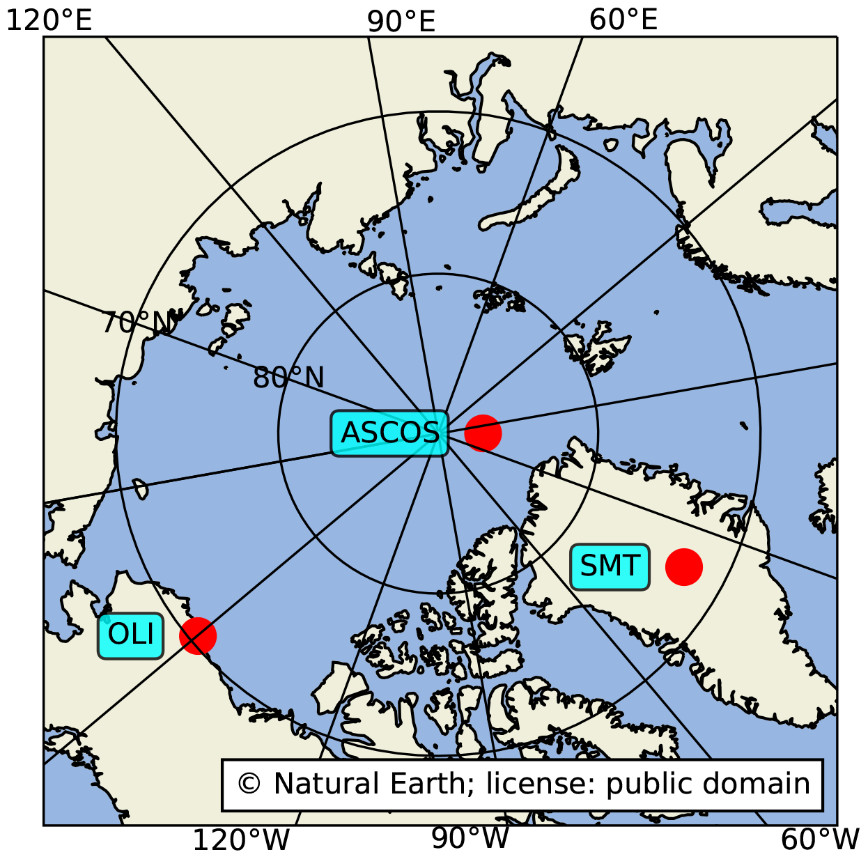
Figure 1 Map showing the locations of data taken from OLI, ASCOS, and SMT.

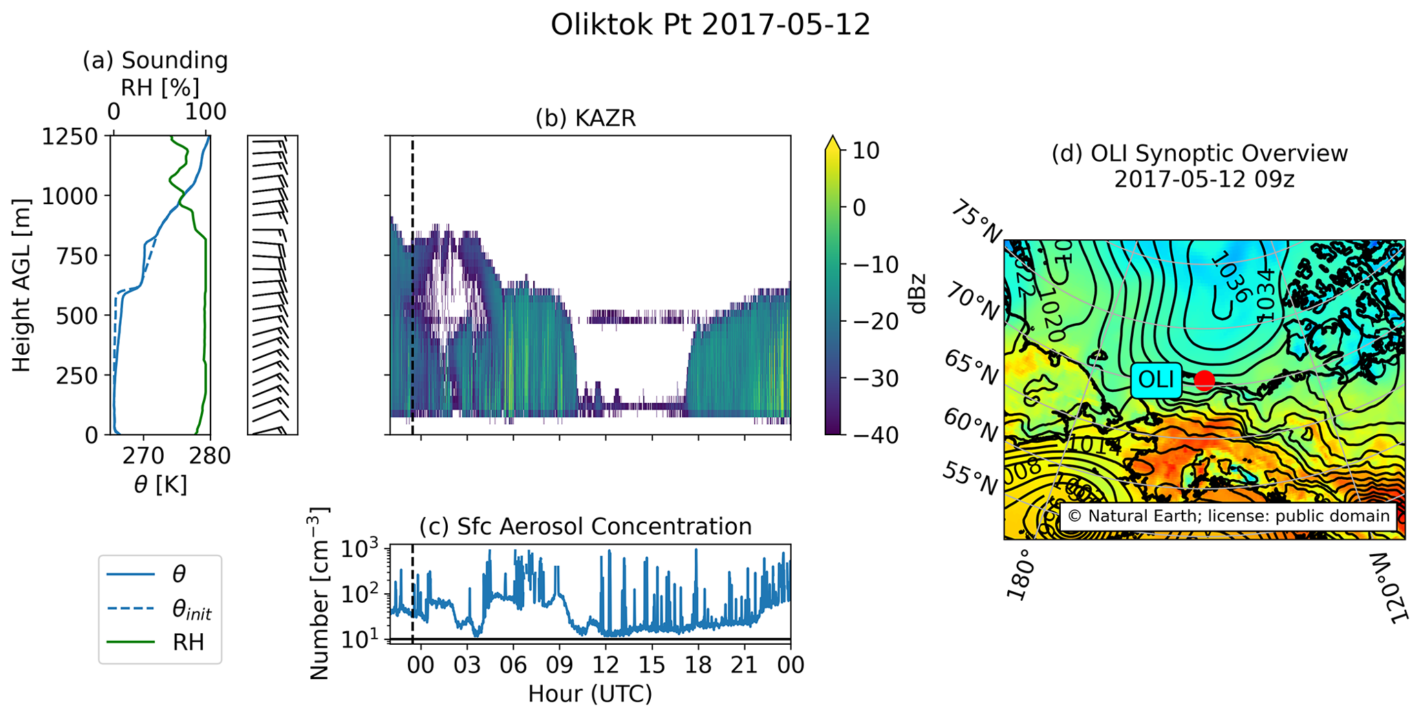
Figure 2 Overview of observations for Oliktok Point, AK (OLI). (a) Potential temperature (θ; blue) and relative humidity (green) and wind barbs from a sounding at 23:30 UTC on 11 May 2017. (b) KAZR (radar) general mode reflectivity (dBz). (c) Surface aerosol concentration (CPC fine). (d) ERA5 reanalysis mean sea level pressure (contours) and 2 m temperature (color shading) for 12 May 2017 at 09:00 UTC. The dashed vertical line in panels (b, c) represent the time at which the sounding was taken. The solid horizontal line in panel (c) represents a surface aerosol concentration of 10 cm⁻¹. For OLI alone, θ_init in panel (a) represents the profile used for the model initialization.

2.1.1 Oliktok Point

From 2013–2021, the United States Department of Energy's Atmospheric Radiation Measurement (ARM) user facility operated a mobile facility at Oliktok Point, Alaska (henceforth OLI), located on the northern Alaskan coastline 260 km southeast of the permanent ARM facility in Utqiaq̇vik. We analyzed data from Oliktok Point between 2016–2019 to find periods in which surface aerosol concentrations via a condensation particle counter (CPC; measuring particles 10–3000 nm; Kuang et al., 2016) were observed to decrease from > 50 to < 20 cm⁻³ in a span of 4 h. Many such periods exist, and the results were examined manually to select cases where this aerosol decrease occurred coincidentally with cloud dissipation seen via radar – signaling that aerosol-limited dissipation may have been a factor in transitioning from a cloudy to cloud-free environment.

One such case (Fig. 2) occurred on the 12 May 2017. At 09:00 UTC, the CPC measured a transition in aerosol concentration from ∼ 100 to  < 10 cm⁻³ in the span of about 1 h (Fig. 2c). Aerosol data from OLI were particularly noisy, with a clear trend of concentrations ∼ 100 cm⁻³ but with intermittent spikes upwards of 1000–10 000 cm⁻³ (not shown). To smooth out the data and best show what we consider to be a representative aerosol concentration time series, we filtered out values > 1000 cm⁻³ and downsampled the result from 1 s to 1 min averages. Data from the Ka-band ARM zenith radar (KAZR; Lindenmaier et al., 2015) show a cloud, with a top at around 700–750 m, transition to clear skies at the same time (Fig. 2b). Around 18:00 UTC, aerosol concentrations begin to increase, and a new cloud is visible on the radar.

The sounding from OLI (Fig. 2a) shows a well-mixed, surface-coupled boundary layer with a capping inversion at 600 m. A second, smaller inversion can be seen at 800 m. However, since this balloon launch occurred approximately 9 h before cloud dissipation, and the radar (Fig. 2b) indicates that the second, higher, cloud layer descends and merges with the lower layer, this second inversion is removed prior to model initialization (θ_init; Fig. 2a; dashed line). Relative humidity (RH) is high (> 90 %) throughout the boundary layer and up to 200 m above the cloud layer before it starts decreasing above 800 m. Aerosol concentrations fluctuate between the time of the sounding and the time of dissipation, so a value of 80 cm⁻³, as a representative average of the pre-dissipation concentration, is used to initialize the simulation.

Surface analysis from ERA5 reanalysis (European Centre for Medium-Range Weather Forecasts, 2019) at 09:00 UTC on 12 May 2017 (Fig. 2d) depicts a high pressure system in the Beaufort Sea north of Oliktok Point and a stationary front situated along the Brooks Range of mountains more than 200 km inland. A weak ridge of high pressure extends from the high pressure system to Oliktok Point, with weak low pressure areas identified to the southeast and southwest of Oliktok Point. This pressure ridge is not present in analysis maps ± 6 h from 09:00 UTC. Analysis of pressure, temperature, and wind time series (not shown) at OLI suggests a weak frontal passage with a temperature drop and wind shift near the same time as cloud dissipation and a constantly decreasing surface pressure throughout the entire 24 h period. It is possible that the change in air mass from a frontal passage was the primary cause of dissipation and surface aerosol concentration decrease. It is also possible that precipitation scavenged aerosol from the below-cloud boundary layer, which could explain the rapid decrease in surface aerosol concentrations.

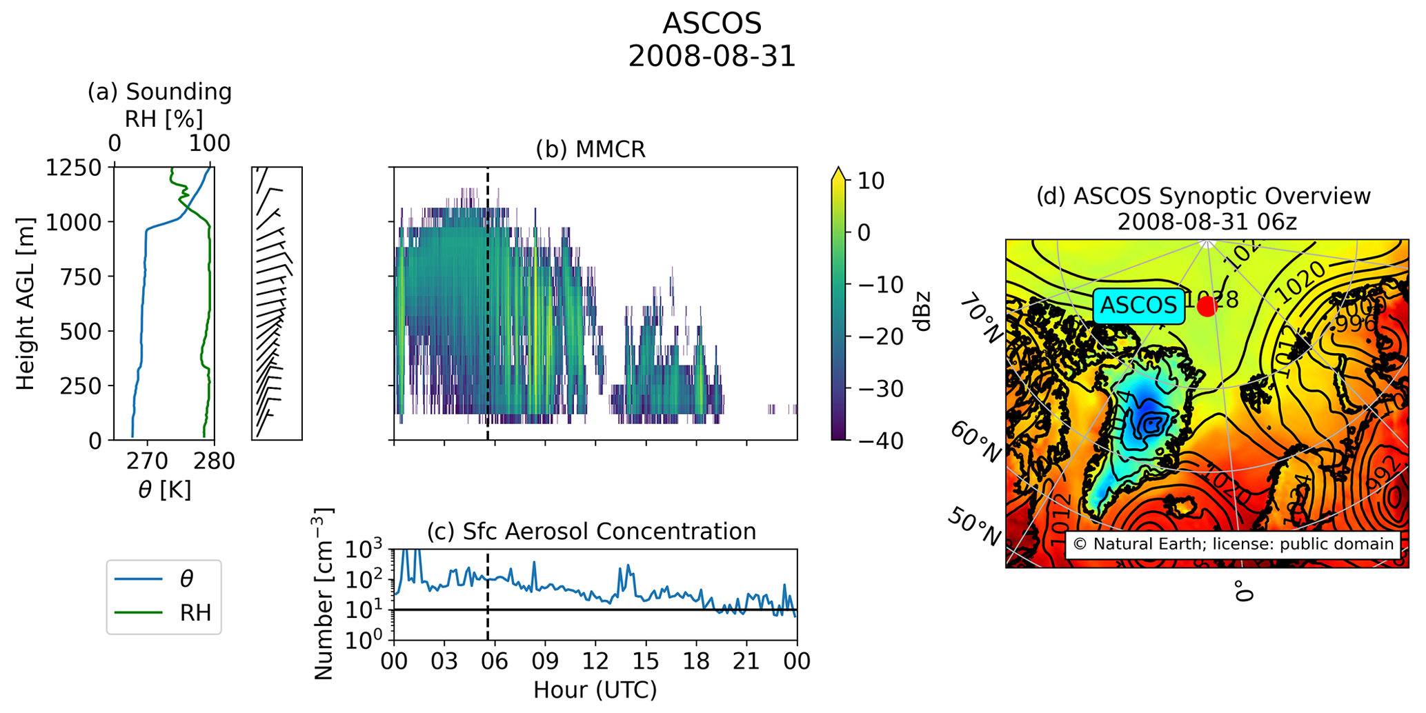
Figure 3 Same as Fig. 2 for the ASCOS case.

2.1.2 ASCOS

The ASCOS field campaign (Tjernström et al., 2014) took place mostly during the month of August 2008, with a focus on observing and understanding Arctic low-level clouds and improving their representation in climate models. From 12 August through 1 September, the Swedish icebreaker Oden was purposefully trapped in (and drifted with) an ice floe in the high Arctic ocean 87^∘ N) north of the island of Svalbard (Fig. 1).

On 31 August 2008, Oden was trapped in an ice floe at 87.19^∘ N, 9.67^∘ W. A sounding from this time (Fig. 3a) shows a slightly stable layer up to 300 m and a well-mixed layer from 300 m to cloud top at 1000 m. Like the OLI case, RH values are generally high throughout the boundary layer. A change in θ and RH profiles at 300 m indicate that the subcloud layer is weakly decoupled from the surface.

This case has previously been investigated as existing in a potentially tenuous regime (Mauritsen et al., 2011; Loewe et al., 2017; Stevens et al., 2018; Tong, 2019). Millimeter-wave cloud radar (Clothiaux et al., 2000) reflectivities show a low-level cloud layer (Fig. 3b), which had persisted for approximately 1 week prior and dissipated coincidentally with a decrease in surface aerosol concentration from > 100 to < 10 cm⁻³ (Sedlar et al., 2011; Mauritsen et al., 2011; Sotiropoulou et al., 2014). Aerosol concentrations were collected using a differential mobility particle sizer (DMPS; Birmili et al., 1999; Tjernström et al., 2014) measuring size distributions of particles between 3 nm–10 µm. Helicopter flights measuring aerosols at 20:13 UTC (after the cloud dissipation) found that concentrations were below 10 cm⁻³ (for aerosols < 14 nm) for the entirety of the boundary layer (Stevens et al., 2018).

After cloud dissipation, winds which were previously calm were observed to blow more consistently from the northeast (not shown). At the same time, surface temperature drops over 6 ^∘C, though it is unclear whether there was a change in air mass or if temperature dropped as cloud is no longer present as a warming influence on the surface. Surface pressure analysis (Fig. 3d) shows the extension of northern high pressure directly over the location of Oden at this time, suggesting a possible change in air mass.

Figure 4 Same as Figs. 2 and 3 for the SMT case.

2.1.3 Greenland

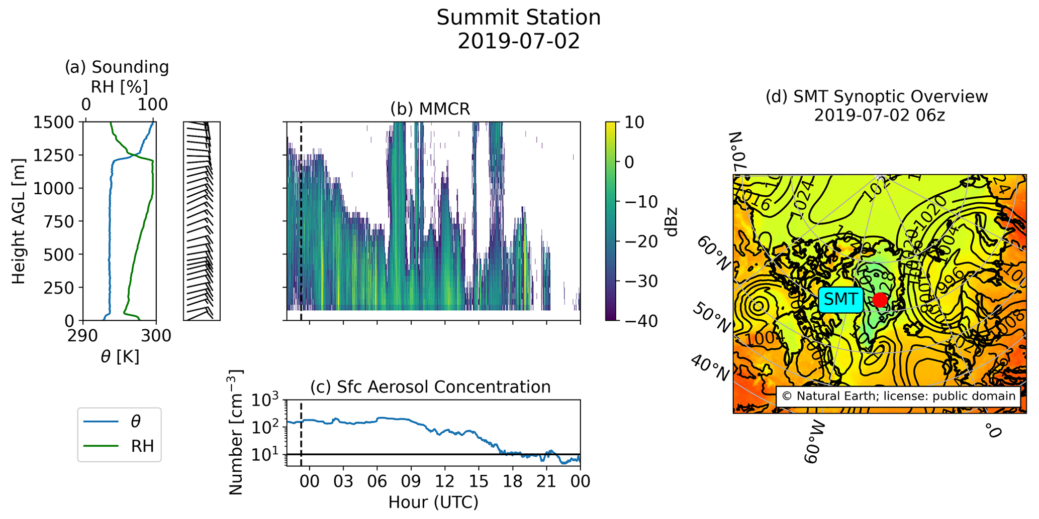
A third case was observed on 2 July 2019 at the National Science Foundation Summit Station (henceforth SMT) during the ICECAPS-ACE project. ICECAPS-ACE (Shupe et al., 2013b; Guy et al., 2021) consists of a suite of instruments for measuring atmospheric properties (including surface aerosol concentrations) at SMT (3250 $\mathrm{m}\mathrm{a}.\mathrm{s}.\mathrm{l}.$; 72.6^∘ N, 38.5^∘ W).

Figure 4 shows an overview of this case, which was first reported in Guy et al. (2021) as an potential example of aerosol-limited dissipation. A well-mixed boundary layer topped with a single cloud layer approximately 200 m in thickness ∼ 1200 m above the surface (∼ 4400 $\mathrm{m}\mathrm{a}.\mathrm{s}.\mathrm{l}.$) is observed with a balloon sounding on the previous day (1 July 2019 at 23:16 UTC; Fig. 4a). Radar data (Fig. 4b) from a millimeter wave cloud radar (Bharadwaj, 2010) show the cloud top lowering before a transition to clear sky as surface aerosol concentrations decrease from 200 cm⁻³ to < 10 cm⁻³ (Fig. 4c) in a period of 9 h (CPC measured particles > 5 nm in diameter in 1 min intervals; Guy et al., 2020). Synoptic conditions at this time show that this case occurred during a period of anomalously low 500 hPa heights and above-average winds from the southeast (Guy et al., 2021, not shown). A small inversion near the surface decouples the boundary layer from surface fluxes of heat and moisture. Unlike OLI and ASCOS, below-cloud RH decreases towards the surface, reaching ∼ 50 % directly above the surface inversion.

2.2 Model description

The Colorado State University Regional Atmospheric Modeling System (RAMS; Cotton et al., 2003) was used to run large eddy resolving simulations (LESs of each case. The RAMS model has been shown to perform well at LES scales (e.g., Cotton et al., 1992; Jiang et al., 2001; Jiang and Feingold, 2006). RAMS uses a two-stream radiation scheme based on Harrington (1997), and turbulence is parameterized by the Deardorff (1980) level-2.5 scheme, which parameterizes eddy viscosity as a function of turbulent kinetic energy (TKE).

RAMS uses a double-moment bulk microphysics scheme (Walko et al., 1995; Meyers et al., 1997; Saleeby and Cotton, 2004) that predicts the mass and number concentration of the following eight hydrometeor categories: cloud droplets, drizzle, rain, pristine ice, aggregates, snow, hail, and graupel. Each of these hydrometeor categories is represented by a generalized gamma distribution. The scheme simulates cloud and ice nucleation, liquid condensation/evaporation, ice deposition/sublimation, collision–coalescence, freezing, secondary ice production (via the Hallett–Mossop process), and sedimentation. Cloud droplets are activated from aerosol particles, using lookup tables (Saleeby and Cotton, 2004) built based on Köhler theory and cloud droplet growth equations formulated in Pruppacher and Klett (1997). Water vapor is depleted from the atmosphere upon activation by assuming that newly activated droplets have a diameter of 2 µm.

Ice crystals are heterogeneously nucleated by the parameterization in DeMott et al. (2010), with the number of ice nuclei (L⁻¹) given by the following:

$$\begin{array}{}\text{(1)}& n_{\text{in}}=a(\mathrm{273.16}-T_{\mathrm{k}}{)}^b(n{)}^{c(\mathrm{273.15}-T_{\mathrm{k}})+d},\end{array}$$

where n_in is the ice nuclei number concentration (L⁻¹), T_k is the air temperature in Kelvin, and $a,b,c,d$ are constants. The variable n in the original DeMott et al. (2010) parameterization is the number concentration (cm⁻³ at standard temperature and pressure) of aerosol particles with diameters larger than 0.5 µm, but in this study, we have elected to use an option in RAMS to set a constant n at model runtime (values of n used are noted in Table 1).

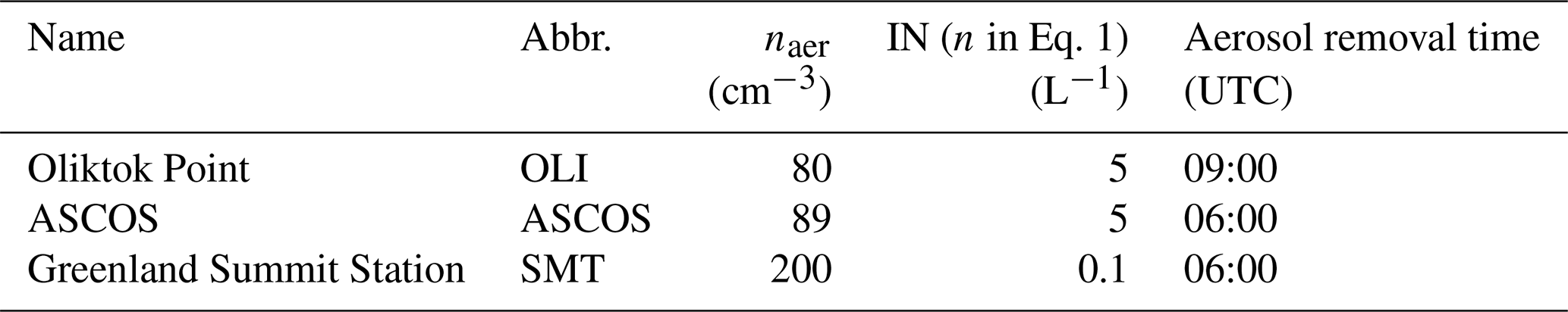
Table 1 Case names and abbreviations (Abbr.) along with the initial aerosol concentration (n_aer), ice nuclei concentration (IN), and aerosol removal time.

2.3 Experiment setup

The observations were used to generate an initial sounding and to specify aerosol concentration for each simulation. For each case, RAMS was run with a horizontal domain of 6 km × 6 km, with a spacing of 62.5 m, and vertical spacing of 6.25 m, with a domain height of 1250 m (200 levels), for OLI and ASCOS and 1600 m domain height (256 levels) for SMT (to accommodate the deeper boundary layer). Lateral cyclic boundary conditions are employed, allowing features that pass through one side of the domain to emerge from the other. While soundings are available at all measurement sites, they do not contain information on the liquid water/ice content of the cloud. To properly initialize RAMS, liquid water was manually added to the sounding data. In the absence of observed vertical profiles of liquid water content, a linear profile of water mass (zero at cloud base and maximum at cloud top) was added, with a slope chosen such that integrating the liquid profile from cloud base to cloud top yielded the observed liquid water path.

In all experiments, the surface is set to ice; surface fluxes are disabled, as they are expected to be low over an icy surface (e.g., Shupe et al., 2013a). Surface albedo was set to 0.5 in ASCOS and 0.6 in OLI and SMT; this is in agreement with albedo measurements taken oven the Arctic which typically range from 0.5–0.7 (e.g., Lindsay and Rothrock, 1994). In addition to cloud liquid added as described above, model initial conditions are provided by sounding height, pressure, potential temperature, humidity, and wind data. Apart from the temperature nudging and prescribed subsidence rate, no other forcings are present. The upper vertical boundary is provided by a Raleigh friction absorbing layer which relaxes horizontal and vertical velocity and potential temperature to their initial values.

We use a simplified aerosol treatment in which number concentrations are fixed to a single value throughout the domain. Aerosol are not depleted; instead, the prescribed number concentration acts as an upper bound on the number of activated cloud droplets allowed in a given grid cell. For each of the cases, we performed simulations in which all aerosol are instantaneously and permanently removed from the environment. We do this in order to simulate the fastest possible cloud dissipation; if the observations show faster dissipation than we simulate, then we can conclude that the observed dissipation was not driven entirely by a lack of aerosol particles.

This aerosol removal only affects cloud droplet nucleation; the highly simplified ice nucleation scheme (as discussed in the section above) is not affected. Since the ice nucleation scheme does not consider different nucleation pathways, removing ice-nucleating particles (INPs) would shut off all ice nucleation, including ice that would have formed via immersion freezing – which has been shown to be the primary ice nucleation method for this type of cloud (Savre and Ekman, 2015). Realistically, INPs immersed within liquid droplets would persist in the presence of the large-scale aerosol decrease that we are modeling here. We ran simulations in which ice nucleation remained active post-aerosol removal and simulations in which ice nucleation was turned off by setting n=0 in Eq. (1) at the aerosol removal time. Both are discussed below, but the focus of the analysis is on the simulations in which ice nucleation remained active post-aerosol removal.

From model initiation to the aerosol removal time, a temperature nudging scheme is used to maintain a stable cloud. Without this nudging, the modeled cloud slowly dissipates (on a timescale of hours) in the absence of large-scale forcings due to gradual radiative cooling and glaciation. The nudging is applied to allow the model enough time to spin-up while maintaining a stable cloud. At each time step, each grid point is linearly nudged back to the initial temperature profile with a timescale of τ = 1 h. Nudging values are computed based on the current domain-averaged temperature profile, so all grid points at a given height z are nudged the same amount. The result in all simulations is a cloud that is quasi-steady in thickness and water content. After the removal of aerosol from the model, the temperature nudging scheme is turned off – this is done so that the post-aerosol thermodynamic environment is able to evolve naturally. That said, the choice to turn off temperature nudging has very little impact on the rate at which the liquid water path decreases post-aerosol removal (not shown). Large-scale subsidence is applied throughout the simulation by imposing a horizontal divergence of 2 × 10⁻⁶ s⁻¹ (set via the name list variable DIVLS) at every model level, with a boundary condition of w_sub = 0 at the surface.

A list of experiments and initial aerosol/ice nuclei concentrations is found in Table 1. Measurements of surface aerosol concentrations were used to initialize the aerosol concentration for each simulation. For ice nuclei (IN) concentrations, we performed sensitivity tests to different values of the n in the IN parameterization (Eq. 1) and found that in OLI and ASCOS there was little change in the liquid water for n = 1, 5, or 10 L⁻¹. There were moderate differences in ice water content, and as there are ice water path (IWP) retrievals for both the OLI and ASCOS cases, we picked a value of n that yielded simulated IWP values closest to observations. For the SMT case, simulated ice and liquid were sensitive to choice of n, so a value of 0.1 L⁻¹ was used; this value is consistent with currently unpublished INP data from Summit Station (available upon request) and resulted in simulated liquid water path that was closest to observations.

3 Results

Figure 5 shows domain-averaged liquid water (color shading), and ice (dashed contours at 0.01 and 0.001 g kg⁻¹) shows typical Arctic mixed-phase clouds in which a layer of supercooled liquid water is situated at cloud top with ice precipitating below. In OLI and ASCOS, the liquid layer is well above the ice layer (∼ 200 m from the cloud top to the 0.001 g kg⁻¹ ice contour), whereas in SMT the ice extends nearly to the cloud top.

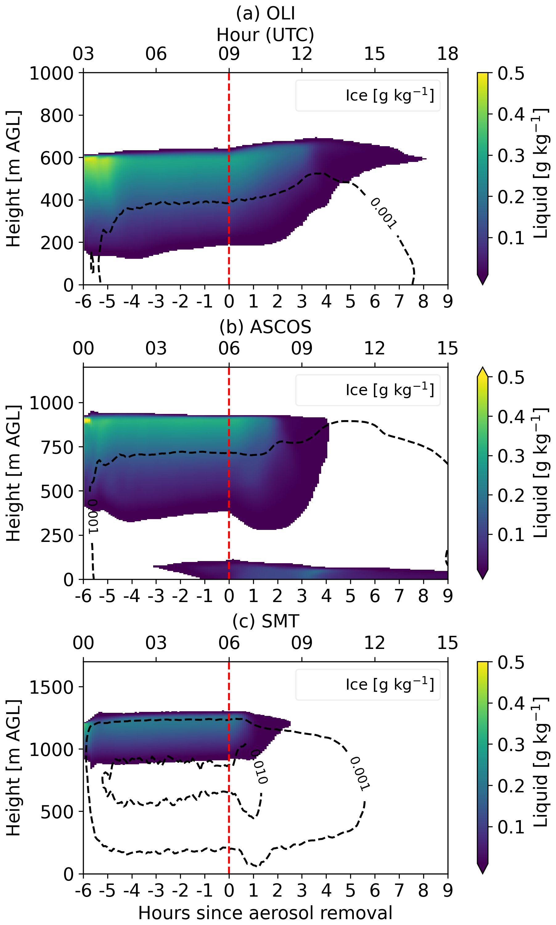
Figure 5 Contours for cloud water (color shading) and ice (dashed) (a) OLI, (b) ASCOS, and (c) SMT simulations. Ice is contoured at 0.01 and 0.001 g kg⁻¹ (the 0.01 g kg⁻¹ contour is only present in c).

Figure 6 shows the domain mean liquid water path (LWP) for the OLI, ASCOS, and SMT simulations and the corresponding observed LWP. The dashed red line denotes the time aerosol were removed. Observed LWP data were taken from microwave radiometers at OLI (Gaustad, 2014), ASCOS (Westwater et al., 2001), and SMT (Cadeddu, 2010). The time at which aerosol were removed from the model was based on a subjective determination from the surface CPC data for each case. The solid orange lines show the LWP of the simulations in which ice nucleation was active past the aerosol removal time, whereas the dashed orange line (IceNucOff) shows the effect of turning off ice nucleation.

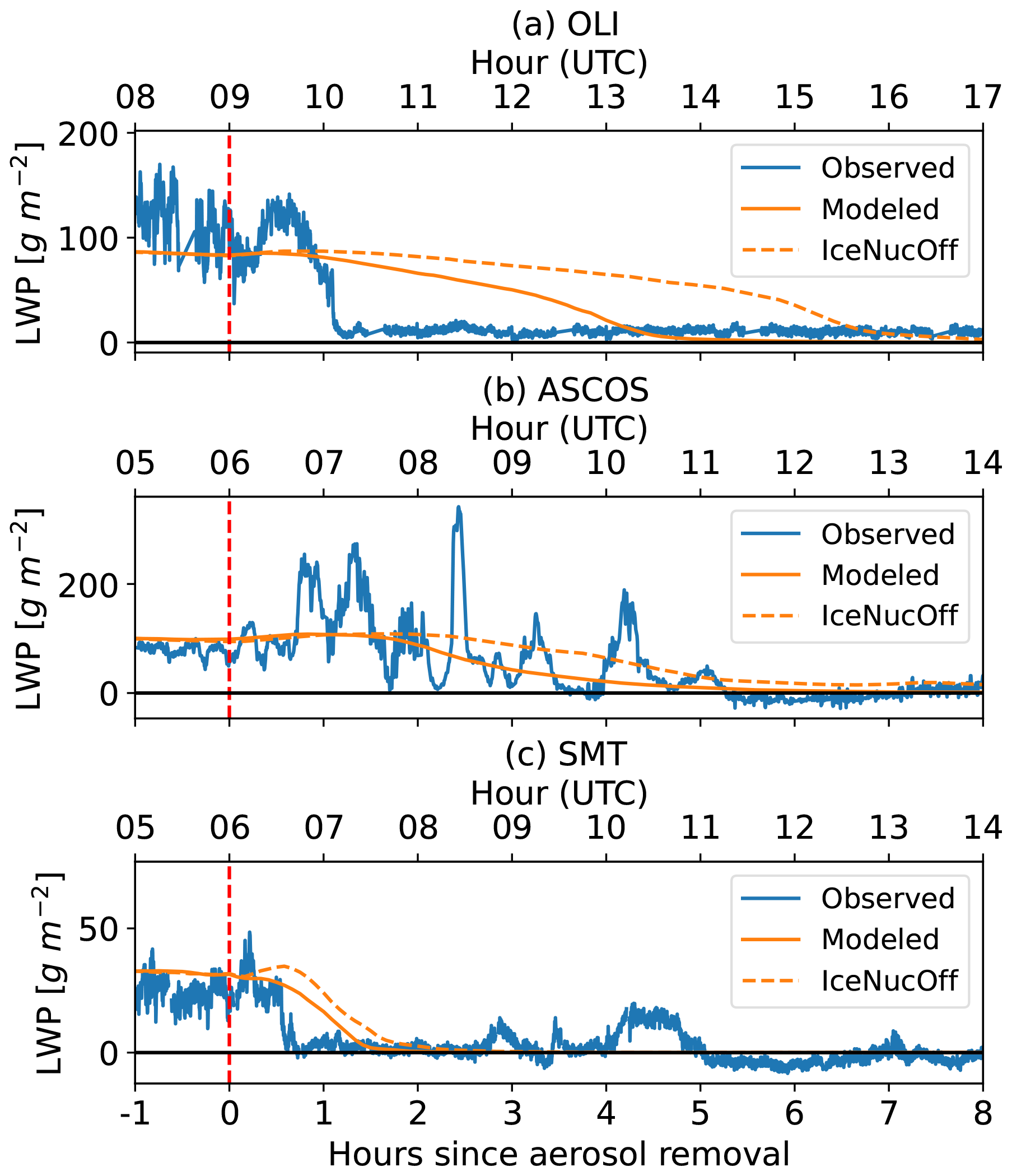
Figure 6 Liquid water path evolution for observations (blue) and modeled domain averages (orange) at (a) OLI, (b) ASCOS, and (c) SMT. The red dashed line denotes the time at which aerosol were removed from the simulations. LWP from simulations in which INP were also removed is shown as dashed orange lines.

In the simulations that maintain ice nucleation (solid orange lines), the simulated LWP decreases to near-zero within hours of the aerosol removal time (09 z in OLI, 06 z in ASCOS and SMT). While the modeled and observed LWP may not line up perfectly, we are concerned primarily with comparing the slopes of the modeled and observed LWP. Both the OLI and ASCOS simulations show a slow LWP response to aerosol removal, with LWP approaching 0 g kg⁻¹ in about 4–5 h. The SMT simulation, on the other hand, has a faster LWP response to aerosol removal, with LWP approaching zero within 2 h. With instantaneous aerosol removal, the simulations represent the fastest possible dissipation of a cloud due to insufficient aerosol. Where this simulated LWP response is slower than observations – such as OLI – it is likely that a lack of aerosol is not in fact the primary driver of dissipation. Where the simulated LWP response is more similar to observations (ASCOS and SMT), it is more likely that these are indeed cases of aerosol-limited dissipation.

In all three simulations, turning off ice nucleation post-removal delays the LWP response by decreasing the amount of ice in the post-removal atmosphere – meaning that liquid processes alone were left to remove available water vapor. However, in both ASCOS and SMT simulations, the resulting LWP decrease has approximately the same slope as the corresponding simulation in which INP were kept active. OLI shows the largest difference in LWP response, with an approximately 50 % increase in the time needed to deplete the cloud of water. Despite this varying change in LWP response with deactivating ice nucleation, we find post-removal liquid budgets for the two ice nucleation treatments show a similar balance between processes in all cases, though post-removal liquid growth was naturally larger in simulations without ice nucleation.

In all simulations, but most pronounced in ASCOS, the subgrid turbulent kinetic energy (TKE, not shown) decreases after cloud dissipation. This is anticipated, as the lack of forcings in our model setup means that there is no mechanism to generate additional turbulent motions after the cloud-generated circulation decomposes. However, by the end of each simulation, much of the subgrid TKE has relaxed completely to the background state, which indicates that the model is no longer resolving large eddies and is no longer operating in the LES regime.

Each case will now be discussed in detail. Since the time of aerosol removal was determined rather subjectively, and because the aim of this paper is not to compare directly with observations but instead to compare timescales, all further discussion of our results will be done in the context of hours before/after aerosol removal, instead of Coordinated Universal Time (UTC), to better compare cases with one another. As stated in Sect. 2.3, we will present only the results where ice nucleation was kept active post-removal in an effort to retain immersion freezing in the simplified ice scheme.

3.1 OLI

It is evident from Fig. 6a that the OLI cloud dissipation was not due to a lack of available aerosol. While the observed LWP decreased from 100 to < 10 g kg⁻¹ in ∼ 1 h, modeled LWP took 4–5× this time. The cause of this is unclear from the available observations, but it might be related to a possible air mass change (outlined in Sect. 2.1.1). While the OLI case may not be a real-world example of aerosol-limited dissipation, examining its simulated response to aerosol removal when compared to the different cases still yields valuable insights to this phenomenon.

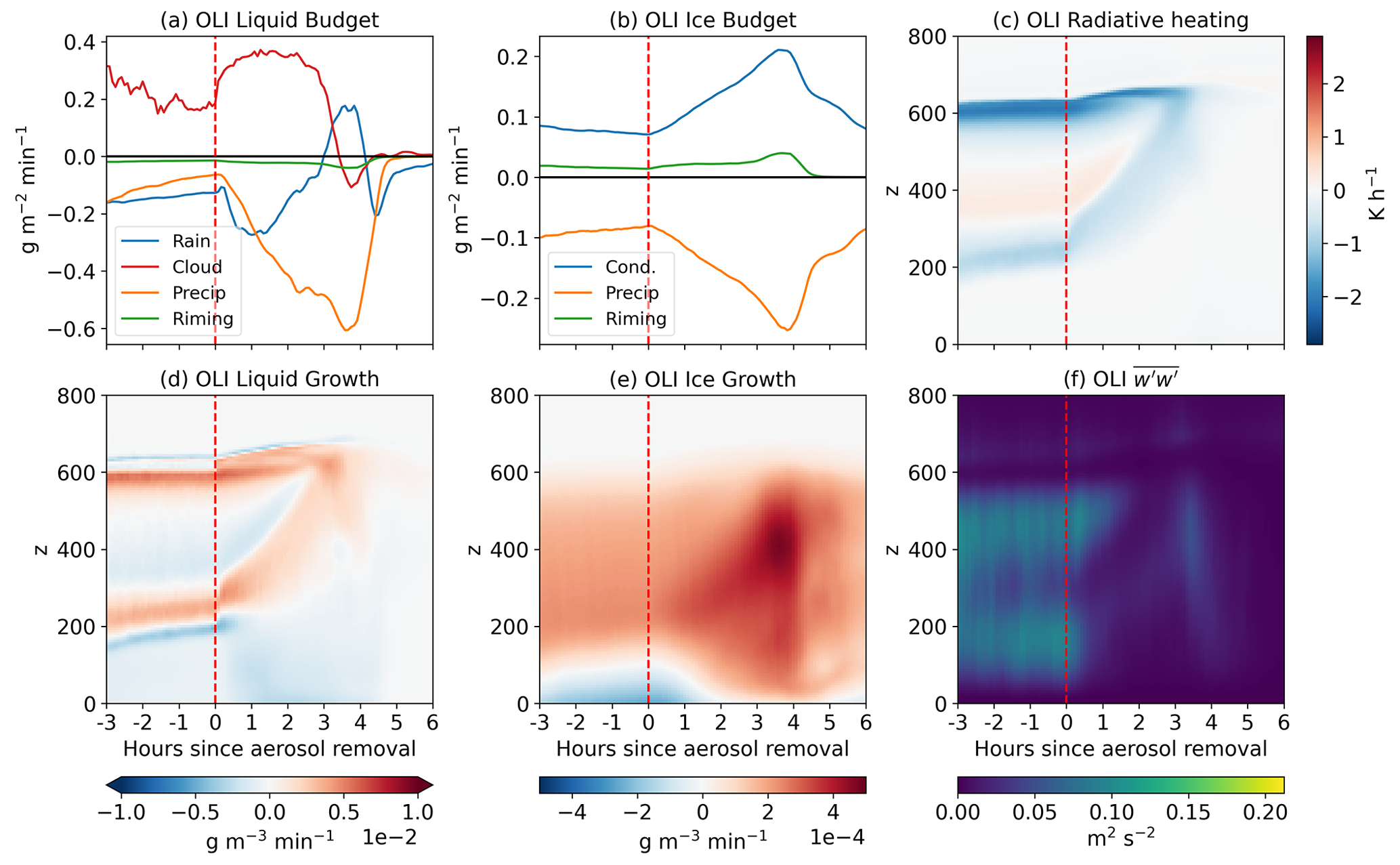
Figure 7 Vertically integrated domain-averaged budgets for (a) condensational growth of liquid hydrometeors (Rain; Cloud), removal by accumulation of liquid precipitation at the surface (Precip) and riming (Riming). (b) Growth of all ice species by condensation (Cond), riming (Riming), and removal by accumulation of ice precipitation at the surface (Precip). Additionally, 2D (time/height) (c) radiative heating/cooling, growth of (d) liquid and (e) ice, and (f) vertical momentum flux for OLI. The red line denotes the time of aerosol removal.

Domain-averaged 2D and column-integrated liquid and ice budgets, radiative heating, and vertical momentum flux for OLI are shown in Fig. 7. After a 1 h spin-up period (not shown), the cloud settles to quasi-equilibrium with approximately constant liquid precipitation reaching the surface and consistently positive integrated cloud droplet growth by condensation, which occurs primarily at cloud base, where supersaturation is largest, and at cloud top. The growth of ice and liquid are balanced by the persistent precipitation of both liquid and ice hydrometeors throughout the pre-aerosol removal time period. Riming makes up only a small part of the liquid and ice budgets. Radiative cooling (Fig. 7c) is strongest at cloud top, as expected, which drives the overturning circulation responsible for maintaining the cloud. Vertical momentum flux ($\stackrel{\mathrm{‾}}{w^{\prime }{w}^{\prime }}$; Fig. 7f) is strongest throughout the mixed portion of the boundary layer – from cloud top down to 100 m.

After the removal of aerosol, a large increase in liquid precipitation and a smaller relative increase in ice precipitation occur. Removing aerosol inhibits the nucleation of new cloud droplets, meaning that any supersaturation must be condensed onto existing droplets rather than being used for nucleation. This results in a rapid increase in droplet sizes (not shown) and an enhanced collision–coalescence process, leading to increased liquid precipitation. The precipitation generation is initially strongest near the cloud base (not shown) and contributes to a rise in cloud base. Since new droplets are unable to be nucleated (and available liquid to condense upon is being precipitated), supersaturation levels increase (not shown). Approximately 3 h after aerosol removal, cloud condensation falls off sharply. Figure 7d and e show that, after aerosol removal, there is an increase in ice growth which maximizes after liquid is mostly removed (Fig. 6a). However, at this point, the cloud top radiative cooling has ceased, circulations weaken, and the ice begins to slowly decay as well.

Figure 5a shows that, after aerosol removal, the OLI simulation dissipates with a rising cloud base and a lesser rising of the cloud top. However, radar observations (Fig. 2b) show a cloud that dissipates with a cloud top that is lowering. After aerosol removal (and temperature nudging is turned off) in the OLI simulation, the entire boundary layer cools and stabilizes (not shown). As a result of this stabilization, turbulence generated by cloud-top cooling is not able to extend as far down as before, resulting in a rising cloud bottom. It is not clear what is causing the cloud top to lower in the observed case; this difference in the modeled versus observed cloud shape during dissipation – combined with the much faster observed LWP response compared to simulations – indicates that the observed dissipation is likely due to larger-scale factors, such as the possible weak frontal passage described in Sect. 2.1.1 or a change in large-scale subsidence. We also speculate that the liquid water profile added to the model initialization results in cloud-top liquid water content (LWC) high enough to produce stronger longwave cooling, which could cause a thermodynamic adjustment that raises the top of the boundary layer. Better constrained large-scale subsidence rates (and their temporal changes), could potentially improve the representation of clouds in our modeling setup.

3.2 ASCOS

The simulated LWP response in ASCOS (Fig. 6b) is much more in line with observations than either of the other two simulations. While there is significant variation in observed LWP between 06:30–11:00 UTC, the modeled LWP fits the downwards trend of these variations quite closely. However, the simulations show that the main cloud layer dissipates almost entirely within about 3 h after aerosol removal and thereafter most of the liquid is contained in a fog layer near the surface (Fig. 5b) that developed prior to aerosol removal. This fog layer may be in line with observations; while not detected by radar, observers reported a fog bow forming in the later hours (UTC) of 31 August (Mauritsen et al., 2011). The radar observations show that the cloud dissipated with a simultaneous drop in cloud top height. The cause is not clear, but it may be a result of ice slowly settling after the liquid is mostly removed, as seen in our simulations. It may also be associated with a change in the large-scale divergence and subsidence rate. Whatever the cause, the drop in cloud top height (as indicated by the presence of either liquid or ice) in the simulations seems to occur much more rapidly. While the observations and simulation are not exactly the same, they seem similar enough that a lack of aerosol particles cannot be ruled out as a cause of the dissipation in the ASCOS case.

Figure 8 Same as Fig. 7 for ASCOS.

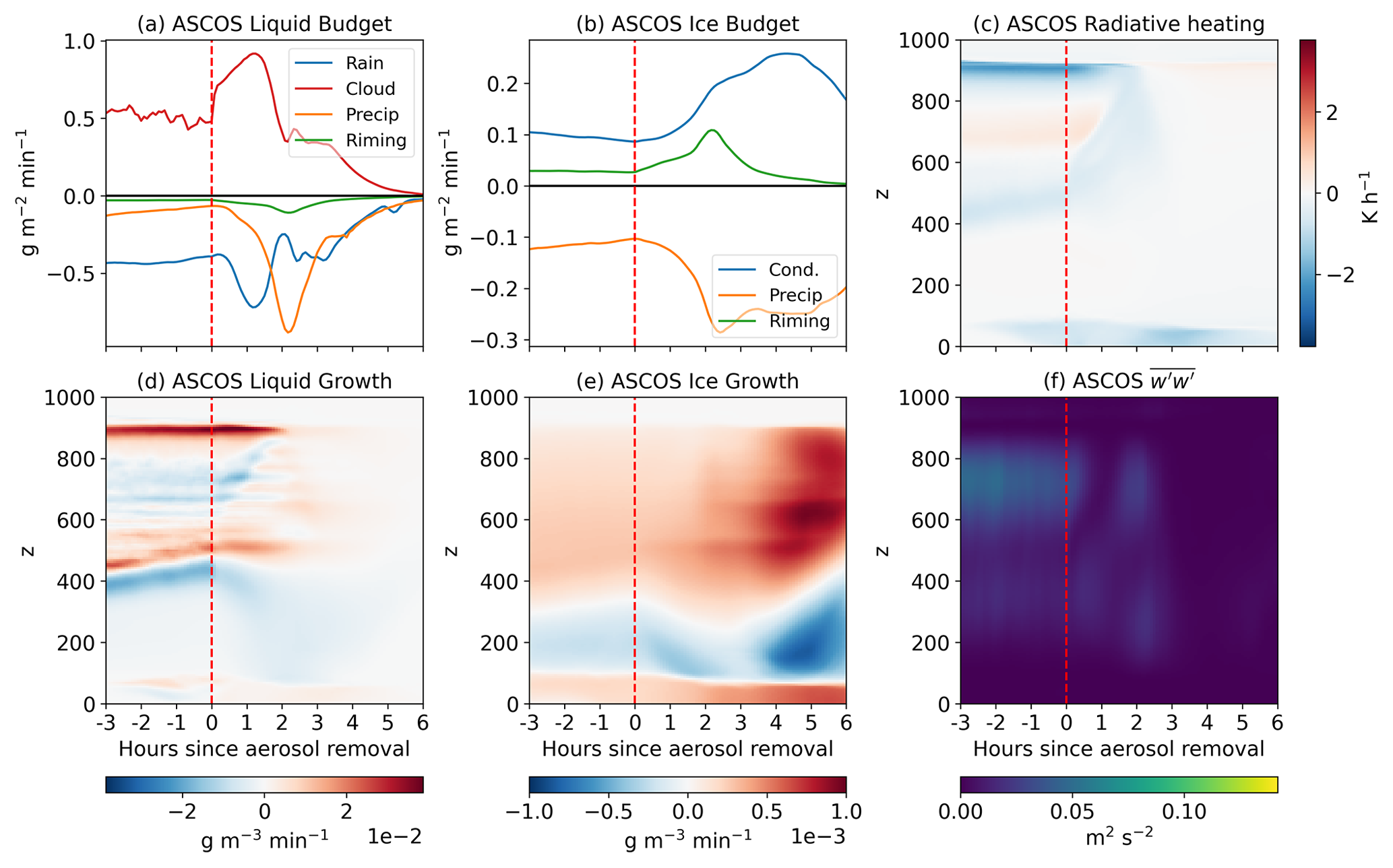
Figure 8 shows the budgets for ASCOS in the same fashion as OLI in Fig. 7. The ASCOS and OLI cases are similar, as both have constant liquid and ice precipitation reaching the surface throughout the pre-aerosol removal period, balancing the positive ice and liquid growth. Both simulations had uniform radiative cooling at cloud top and weak heating or cooling elsewhere. Unlike OLI, the ASCOS simulation was initialized with a sounding where the boundary layer was decoupled from the surface from a temperature inversion around 300 m (Fig. 3a). As a result, the vertical turbulent momentum flux (Fig. 8f) is weaker and does not extend as far below the cloud as in OLI (Fig. 7f).

Much like OLI, once aerosol are removed from the environment, there is a sharp increase in cloud condensational growth, leading to a large amount of liquid precipitation and rain evaporation. Shortly after this rise in liquid condensation, ice growth rates almost triple at 09:00 UTC. Simultaneously, liquid growth drops sharply. While initially this may seem to indicate the WBF process glaciating a cloud, investigating the growth budget in 2D (time/height; Fig. 8d and e) shows that there is typically net condensation of liquid in the cloud layer after aerosol removal. However, liquid growth (while remaining positive) is still decreased significantly in the location of maximal ice growth, so it appears that both liquid and ice processes are competing for available water vapor. As liquid droplets and ice crystals grow, collide, and fall out as precipitation, this moisture is removed from the atmosphere, and eventually no supersaturation exists with which to grow any hydrometeors. Like OLI, precipitation processes seem to drive the liquid dissipation and the post-removal boundary layer cools throughout (not shown). However, due to the existing decoupled nature of the boundary layer, the effect of this stabilization on the turbulence of the cloud is weakened compared to OLI. As a result, while a slight cloud base rising is observable in, for example, Fig. 8c, it is not as pronounced as in OLI.

3.3 SMT

The SMT simulation is notably different from the other two, with simulated LWP reaching near-zero values within only 2 h of aerosol removal (Fig. 6c). Observed LWP values are near-zero by 07:00 UTC, but radar returns are detected for the next several hours. Based on images taken from the measurement site and micropulse LIDAR depolarization ratios (not shown), it is likely that the radar returns detected after 07:00 UTC are primarily due to near-surface ice fog and not to the presence of liquid water. LWP values are more variable after 09:00 UTC, but this is most likely due to higher-level liquid clouds passing overhead (which can also be seen on radar in Fig. 4b; see Guy et al., 2021, for more analysis of these observations). Radar also shows a cloud whose top is lowering, but Fig. 5c shows little lowering of the cloud top.

Figure 9 Same as Figs. 7 and 8 for SMT.

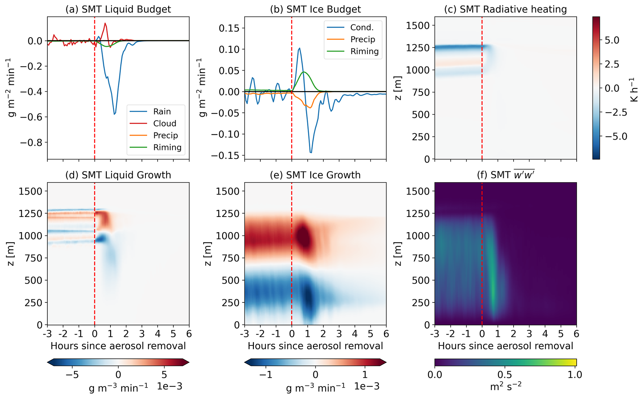
Figure 9 shows the liquid and ice budget, radiative heating rate, and vertical turbulent momentum flux for the SMT case. Radiative cooling at cloud top is about twice as strong (∼  4 K h⁻¹) as in ASCOS or OLI (∼  2 K h⁻¹). This is in agreement with previous studies, which show that an increase in aerosol (200 cm⁻³ in SMT versus 80 and 89 cm⁻³ in OLI and ASCOS, respectively) leads to enhanced maximum cloud-top cooling in Arctic clouds (e.g., Williams and Igel, 2021). The SMT sounding used to initialize RAMS (Fig. 4a) was well mixed from the cloud top to near the surface, so turbulent momentum fluxes are able to consistently extend down to about 200 $\mathrm{m}\mathrm{a}.\mathrm{s}.\mathrm{l}$. As a result of the stronger cooling at cloud top, vertical momentum flux ($\stackrel{\mathrm{‾}}{w^{\prime }{w}^{\prime }}$; Fig. 9f) at SMT is ∼ 0.75 m² s⁻² – approximately 10× stronger than seen in OLI or ASCOS.

Unlike the other two cases, the simulated SMT cloud reaches a different equilibrium pre-aerosol removal. Instead of a balance between cloud droplet/ice growth and precipitation, like in OLI and ASCOS (Figs. 7 and 8), the SMT cloud is balanced by cloud droplet growth at cloud top and cloud base but cloud droplet evaporation in the interior and along the top and bottom edges (Fig. 9c). There was no liquid precipitation or rain evaporation prior to aerosol removal.

Similarly, column-integrated ice growth fluctuates around zero prior to aerosol removal, unlike in the other two simulated cases (Fig. 9b). While there is significant ice production and growth in-cloud (Fig. 9e), it is balanced out by a near-total sublimation below the cloud (Fig. 9e), in part due to the much drier below-cloud boundary layer seen in SMT (Fig. 4a) compared to OLI and ASCOS (Figs. 2 and 3). While some ice precipitation did accumulate on the surface (Fig. 9b; orange line), that removal from precipitation mirrors the addition of ice due to riming, with precipitation being slightly lower due to sublimation of the rimed ice while falling through the below-cloud atmosphere.

Another difference between OLI/ASCOS and the SMT simulation is the location of the ice relative to the liquid layer. In OLI and ASCOS, there was a more distinct separation between the liquid layer and the ice precipitation below it (Fig. 5). In SMT, by contrast, ice is present throughout the liquid layer. This creates more competition between the liquid and ice phases in the cloud.

After aerosol removal there is a short period of rain/drizzle production, though most droplets evaporate or rime before reaching the surface; this increase in rain is not visible as precipitation but instead as rain evaporation in Fig. 9a and riming in Fig. 9b. The areas of liquid evaporation shortly after 06:00 UTC at ∼ 750 m are coincident with strong ice growth (Fig. 9e), suggesting some role of the WBF process in dissipating the cloud. However, this is not necessarily the case. The enhanced negative liquid growth in Fig. 9d occurs at and below cloud base. Cloud droplets grow in the net by condensation (Fig. 9a; red line), and rain evaporation becomes the largest sink of liquid water (blue line). This indicates that the removal of aerosol is promoting development of rain-sized liquid drops which are falling out but not actually reaching the surface (as there is no surface accumulation visible in Fig. 9a). After a very short amount of time (< 1 h), the ice hydrometeors large enough to precipitate do so, and both ice and liquid evaporate. This is in contrast to the other two cases, where ice growth was always positive.

SMT also had less initial liquid water than the other two simulations (∼ 30 g m⁻² compared to ∼ 100 g m⁻² in both OLI and ASCOS), which also may explain why this cloud dissipated faster as there was less than half the amount of liquid water that needed to be removed from the atmosphere. Post-removal, the boundary layer cools much like OLI and ASCOS (not shown). However, in contrast to those two cases, the boundary layer remained well mixed for the first hour and becomes more stable around 08:00 UTC – 2 h after aerosol removal and at which point the cloud has mostly dissipated. As a result, turbulent vertical motions extend quite far throughout the boundary layer (Fig. 9f). This, combined with the stronger turbulence generated by enhanced cooling at cloud top and the drier atmosphere above and below cloud, means that dry air is more readily entrained into the environment and may have been a reason why dissipation occurred so much more quickly. The increased vertical momentum flux seen immediately after aerosol removal (Fig. 9f) may be due to drag from precipitating raindrops.

4 Discussion and conclusions

We investigate the role of low aerosol concentrations on the dissipation of Arctic mixed-phase clouds by running semi-idealized LESs of three different cases in different locations – Alaska's northern coast (OLI), an Arctic Ocean ice floe (ASCOS), and Greenland's Summit Station (SMT). Each LES is initialized based on observations, and aerosol concentrations are instantaneously forced to 0 cm⁻³ at a specified time. Comparing the simulated LWP to observations (Fig. 6), we are able to determine whether it is possible that each observed case dissipated due to a lack of aerosol. By removing all aerosol instantaneously and preventing the model from nucleating new hydrometeors, we effectively simulate the fastest possible response to a lack of aerosol. A case that is observed to dissipate faster than its simulation, in this setup, is likely to have other factors driving the dissipation. We find OLI to be one such case. Cases where the observed LWP response is similar to the modeled response are more likely to be actually caused by a lack of aerosol than those whose modeled LWP diverge further from observations. The ASCOS and SMT cases fall into this first category. While noisy, the observed ASCOS LWP trend lines up very well with the simulated LWP. The SMT case is less certain, and while the observed LWP decreases faster than the simulated values, some factors (such as less certain/accurate representativeness of this cloud setup in the model) may explain the difference. It should be stressed that any LWP agreement between observations and simulations does not, on its own, prove with any certainty the existence of aerosol-limited dissipation in a given case. We argue that, given their simulated LWP, the ASCOS and SMT cases should be investigated further as possible cases of aerosol-limited dissipation. Avenues for further study include simulations with more realistic aerosol treatment, exploring the relative impact of above and below cloud aerosol on dissipation, and investigating the role of IN entrainment

Our simulations revealed two pre-aerosol removal equilibrium balance states which respond differently to aerosol removal. The first, seen in OLI and ASCOS, results in a continually precipitating cloud in both ice and liquid, where droplet growth is balanced by loss through collisions resulting in removal by precipitation. Conversely, the second balance state (seen in SMT) occurred in a thinner, colder cloud with no liquid precipitation and very little ice precipitation. Instead, liquid and ice coexist in a larger area in SMT (Fig. 5), creating more competition for the available water vapor. The stronger turbulent motions caused by enhanced cloud-top cooling in SMT may have caused the relatively drier above-cloud air to be mixed and entrained into the cloud, also prohibiting the development of large enough supersaturations needed for constant growth.

In addition, we found little difference in microphysical response to aerosol removal between a previously coupled boundary layer (OLI) and a decoupled one (ASCOS). SMT and ASCOS both had decoupled boundary layers, and SMT showed a very different response to aerosol removal than both OLI or ASCOS. We believe that, given the evidence from these three simulations, the microphysical balance state of the cloud may be more important to determining the response to aerosol removal than boundary layer properties. This conclusion, however, is bounded by the limited selection of cases and choices of model setup in this work – such as the lack of surface fluxes in the model, all cases taking place during polar day, identical large-scale divergence imposed on all simulations, and weak wind shear observed in all cases. Future work on this subject could involve testing various boundary layer thermodynamic initial conditions (e.g., coupled/decoupled surface), surface fluxes, etc., and their effects on post-aerosol removal processes.

Understanding Arctic energy balances are paramount to studying the Earth's climate as a whole. Low-level mixed phase clouds have been shown be a large regulator on the Arctic climate, and understanding these clouds and their processes is important to furthering our understanding and modeling ability of weather and climate. While we believe aerosol-limited dissipation in the Arctic to be an uncommon (if not rare) event, understanding the impact of a pristine Arctic environment and how it might change in a more polluted future will be necessary steps in researching Earth's climate change and its impacts.