Albedo susceptibility of northeastern Pacific stratocumulus: the role of covarying meteorological conditions

Quantification of the radiative adjustment of marine low clouds to aerosol perturbations, regionally and globally, remains the largest source of uncertainty in assessing current and future climate. One of the important steps towards quantifying the role of aerosol in modifying cloud radiative properties is to quantify the susceptibility of cloud albedo and liquid water path (LWP) to perturbations in cloud droplet number concentration (N_d). We use 10 years of spaceborne observations from the polar-orbiting Aqua satellite to quantify the albedo susceptibility of marine low clouds to N_d perturbations over the northeast (NE) Pacific stratocumulus (Sc) region. Mutual information analysis reveals a dominating control of cloud state (e.g., LWP and N_d) on low-cloud albedo susceptibility, relative to the meteorological states that drive these cloud states. Through a LWP–N_d space decomposition of albedo susceptibilities, we show clear separation among susceptibility regimes (brightening or darkening), consistent with previously established mechanisms through which aerosol modulates cloud properties. These regimes include (i) thin non-precipitating clouds (LWP < 55 g m⁻²) that exhibit brightening (occurring 37 % of the time), corresponding to the Twomey effect; (ii) thicker non-precipitating clouds, corresponding to entrainment-driven negative LWP adjustments that manifest as a darkening regime (36 % of the time); and (iii) another brightening regime (22 % of the time) consisting of mostly precipitating clouds, corresponding to precipitation-suppression LWP positive adjustments. Overall, we find an annual-mean regional low-cloud brightening potential of 20.8±2.68 W m⁻² ln(N_d)⁻¹, despite an overall negative LWP adjustment for non-precipitating marine stratocumulus, owing to the high occurrence of the Twomey–brightening regime. Over the NE Pacific, clear seasonal covariabilities among meteorological factors related to the large-scale circulation are found to play an important role in grouping conditions favorable for each susceptibility regime. When considering the covarying meteorological conditions, our results indicate that for the northeastern Pacific stratocumulus, clouds that exhibit the strongest brightening potential occur most frequently within shallow marine boundary layers over a cool ocean surface with a stable atmosphere and a dry free troposphere above. Clouds that exhibit a darkening potential associated with negative LWP adjustments occur most frequently within deep marine boundary layers in which the atmospheric instability and the ocean surface are not strong and warm enough to produce frequent precipitation. Cloud brightening associated with warm-rain suppression is found to preferably occur either under unstable atmospheric conditions or humid free-tropospheric conditions that co-occur with a warm ocean surface.

1 Introduction

Changes in aerosol concentrations in the marine boundary layer, of either natural or anthropogenic origin, can lead to significant changes in the brightness of marine low-level clouds. Examples of aerosol-induced changes in cloud reflectivity are observed in aerosol perturbations associated with natural causes, such as volcanic eruptions (e.g., Gassó, 2008; Yuan et al., 2011; Malavelle et al., 2017), and anthropogenic sources across the globe, such as ship emissions, wildfires, and power plants (Toll et al., 2019). Among anthropogenic sources, ship tracks – bright linear cloud features associated with particle emissions (Coakley et al., 1987) – have been used to improve our understanding of cloud responses to aerosol perturbations. The routine and frequent occurrence of global shipping traffic together with constant meteorological conditions in ship tracks and out of ship tracks make them a natural laboratory to help improve our understanding of cloud responses to aerosol perturbations. Studies based on satellite observations (e.g., Coakley and Walsh, 2002; Gryspeerdt et al., 2019b; Chen et al., 2012; Christensen and Stephens, 2011; Christensen et al., 2014) and idealized frameworks such as large-eddy simulations (e.g., Wang et al., 2011; Hill et al., 2009) have been used to improve the quantification of the global aerosol radiative effect (e.g., Diamond et al., 2020). However, to date, our ability to narrow down estimates of climate sensitivity is still limited by uncertainties related to quantifying the radiative adjustment of marine low clouds to the anthropogenic aerosol (Bellouin et al., 2020).

For non-precipitating warm clouds exhibiting constant liquid water path (LWP), increases in aerosol concentration result in increases in droplet concentration (N_d), leading to smaller droplets that make the cloud more reflective (the Twomey effect; Twomey, 1974, 1977). These processes occur at short timescales (on the order of 5–10 min; supplementary materials in Glassmeier et al., 2021). However, LWP is not always constant: LWP adjustments were first suggested to exist in precipitating marine warm clouds – an increase in N_d leads to smaller cloud droplets that are less likely to grow by collision–coalescence to precipitation-sized raindrops under the same environmental conditions (Albrecht, 1989). The result is a reduction in the loss of cloud water due to precipitation, which then leads to an increase in LWP that enhances cloud brightening associated with the smaller drops.

More recently, negative LWP adjustments in non-precipitating stratocumulus have also been identified: (i) the reduced droplet sizes decrease the sedimentation flux at stratiform cloud tops, enhancing the evaporative and radiative cooling and thereby the entrainment rate at cloud tops (the sedimentation-entrainment feedback; Ackerman et al., 2004; Bretherton et al., 2007); (ii) smaller cloud droplets evaporate faster, leading to stronger cooling and more turbulent mixing at cloud tops, which then causes more evaporation, creating a positive feedback loop, known as the evaporation–entrainment feedback (Wang et al., 2003; Xue and Feingold, 2006; Jiang et al., 2006). Both of these entrainment feedbacks reduce cloud LWP in response to the increased concentration of smaller droplets, resulting in fewer reflective clouds and hence a warming relative to a cloud with constant LWP. A strong offsetting warming effect from the negative LWP adjustment is evident in both observational studies (e.g., Chen et al., 2014; Possner et al., 2020; Gryspeerdt et al., 2019a, 2021) as well as large eddy simulation (e.g., Wang et al., 2003; Ackerman et al., 2004; Xue et al., 2008). The timescale associated with these negative LWP adjustments is t≈ 20 h (Glassmeier et al., 2021). Because ship tracks exist for only 6 to 7 h, typically, and are likely to be sampled on average after ∼3 h, a generalization of ship track characterized aerosol–cloud interactions to estimates of anthropogenic aerosol climate forcing may be substantially overestimated because the ship track has not existed for long enough to manifest full negative LWP adjustment (Glassmeier et al., 2021).

Moreover, despite routine shipping traffic, ship tracks are only rarely observed over major shipping corridors (only 0.002 % of the total oceangoing ship traffic; Campmany et al., 2009), in part due to the narrow range of meteorological conditions required for these bright tracks to form (Durkee et al., 2000). This suggests that the coupled large-scale meteorology and the associated cloud states have a strong impact on the susceptibility of low clouds to aerosol perturbations. Several studies have tried to constrain the uncertainties in LWP and reflectance adjustments based on cloud states and large-scale meteorological conditions using satellite observations (e.g., Chen et al., 2014; Douglas and L'Ecuyer, 2019; Possner et al., 2020) and found strong meteorological controls on cloud state and cloud albedo susceptibility to aerosol perturbations across the globe: regions with relative dry and unstable conditions tend to be characterized by cloud darkening in response to increased aerosol loading, whereas clouds in stable and moist regions tend to brighten in response to increased aerosol concentrations.

In order to understand and disentangle the impact of individual meteorological drivers, subsampling of data is often applied in these studies to help constrain the degree of freedom of the system within one meteorological variable by limiting that within the other meteorological variables. This results in minimizing and suppressing the influence of the covariability among meteorological drivers, even though large-scale meteorological conditions are spatiotemporally correlated, especially over the eastern subtropical oceans (e.g., Klein and Hartmann, 1993; Eastman et al., 2016). Thus, the “untangling” leads to neglect of important information, i.e., the frequency at which certain environmental conditions co-occur in nature, which profoundly drives the overall radiative impacts of aerosol–cloud interactions. A shift in attention from untangling aerosol and meteorological effects on cloud systems towards embracing and understanding the covariabilities between aerosol and meteorological drivers has been suggested by Mülmenstädt and Feingold (2018). It is the approach adopted here.

In this work, we focus on the potential radiative impact of “intrinsic” cloud adjustments (due to changes in N_d and LWP). “Extrinsic” cloud adjustment (cloud fraction responses) is not addressed here. We quantify relationships between cloud albedo (A_c) and N_d using satellite-retrieved cloud properties and radiative fluxes (Sect. 2), following the conceptual framework of using N_d as an intermediate variable to minimize the influence of confounding meteorology on the causal relationship between aerosol and cloud as in Gryspeerdt et al. (2016, 2019a). Our target area is the northeast Pacific marine stratocumulus deck, one of the regions contributing most strongly to the overall cooling of the Earth by reflecting incoming solar radiation (Klein and Hartmann, 1993). Cloud albedo susceptibilities are approximated by regressed log-linear relationships between N_d and A_c within a given satellite snapshot, similar to Painemal (2018), assuming processes are related to the current state of the system captured by the satellite snapshot, with no memory of past states (Sect. 3). One should note that this Markovian approach of inferring process from composites of satellite snapshots ought to be restricted to informing relationships between cloud properties from a climatological perspective where a sufficient amount of sampling of a time–space varying system creates a robust characterization of the relationships between quantities that describe the system. This contrasts with approaches targeted at the non-Markovian aspect of the system, i.e., quantifying the time derivatives of cloud properties, through tracking properties of the system, either by numerical simulation or temporally resolved satellite observations (e.g., Glassmeier et al., 2021; Christensen et al., 2020).

The findings of this study (Sects. 4 and 5) feature two key perspectives: (i) the usage of the LWP–N_d parameter space, supported by mutual information analyses (Sect. 4.1), helps to show clear separation between albedo susceptibility regimes that can be linked to physical mechanisms associated with aerosol effects on low clouds (Sect. 4.2 and 4.3); (ii) distinguished from previous work that minimized the covariability between meteorological drivers (e.g., Douglas and L'Ecuyer, 2019), this study adopts a top-down approach that embraces the covariability among meteorological factors (obtained from ERA5 reanalyses) while identifying conditions under which clouds are more (or less) susceptible to aerosol perturbations and quantifying the frequency of occurrence of these conditions (Sect. 5).

2 Datasets

This study focuses on an area of 10^∘ by 10^∘ (20–30^∘ N, 120–130^∘ W) over the subtropical Northeast (NE) Pacific stratocumulus region, corresponding to an area of regional maximum in annual stratus cloud amount, which is the same region examined in Klein and Hartmann (1993). Marine low-cloud properties and shortwave (SW) radiative measurements are retrieved from the Moderate Resolution Imaging Spectroradiometer (MODIS) (Platnick et al., 2003) and the Clouds and the Earth's Radiant Energy Systems (CERES; Wielicki et al., 1996) sensors aboard the Aqua satellite (overpass ∼ 13:30 local time), obtained from the CERES Single Scanner Footprint (SSF) product edition 4 (level 2; Su et al., 2015). Top-of-atmosphere (TOA) SW fluxes, including incoming solar radiation (SW${}_{{\mathrm{TOA}}_{\mathrm{dn}}}$) and reflected SW flux (SW${}_{{\mathrm{TOA}}_{\mathrm{up}}}$), are derived from the single scanner at a CERES footprint resolution of 20 km (Loeb et al., 2005; Su et al., 2015), which are then used to calculate cloud SW albedo (A_c) as follows:

$$\begin{array}{}\text{(1)}& A_{\mathrm{c}}={\displaystyle \frac{(A_{\mathrm{all}}-A_{\mathrm{clr}}(\mathrm{1}-f_{\mathrm{c}}\left)\right)}{f_{\mathrm{c}}}},\end{array}$$

where A_all is scene albedo (all-sky albedo), defined as the ratio of SW${}_{{\mathrm{TOA}}_{\mathrm{up}}}$ to SW${}_{{\mathrm{TOA}}_{\mathrm{dn}}}$; A_clr is the solar zenith angle (SZA)-dependent ocean albedo (clear-sky albedo), derived from the scene albedo under clear-sky conditions over the study area; and f_c is the cloud fraction.

MODIS cloud properties, including cloud optical depth (τ), cloud-top effective radius (r_e), f_c, LWP, cloud effective temperature, and cloud-top height (CTH), are retrieved using the CERES–MODIS algorithm at MODIS pixels and then aggregated to the CERES footprint resolution (20 km) and scanning pattern (Minnis et al., 2011b, a). Retrieval of r_e is based on the 3.7 µm channel, which has been shown to be less affected by retrieval biases than the 2.1 and 1.6 µm channels (Grosvenor et al., 2018). N_d is calculated following Grosvenor et al. (2018) as

$$\begin{array}{}\text{(2)}& N_{\mathrm{d}}={\displaystyle \frac{\sqrt{\mathrm{5}}}{\mathrm{2}\mathit{\pi }k}}({\displaystyle \frac{f_{\mathrm{ad}}{c}_w(T,P)\mathit{\tau }}{Q_{\mathrm{ext}}{\mathit{\rho }}_{\mathrm{w}}{r}_{\mathrm{e}}^{\mathrm{5}}}}{)}^{\mathrm{1}/\mathrm{2}},\end{array}$$

where k is a parameter representing the width of the modified gamma droplet distribution (assumed to be 0.8; Martin et al., 1994); f_ad is the adiabatic fraction (assumed to be 0.8); c_w is the condensation rate, which is a function of temperature (T) and pressure (P) (Grosvenor and Wood, 2014), calculated using CERES–MODIS cloud effective temperature at a constant pressure of 900 hPa; Q_ext is the extinction efficiency factor, approximated by its asymptotic value of 2 (Grosvenor et al., 2018); and ρ_w is the density of liquid water. In addition, N_d is only calculated for CERES footprints with f_c>0.99 (overcast footprints), cloud effective temperature greater than 273 K (to exclude mixed-phase and ice clouds), CTH less than 3 km, τ>3, r_e>3 µm, and SZA $<{\mathrm{65}}^{\circ }$, to minimize retrieval biases (Painemal et al., 2013; Grosvenor and Wood, 2014; Grosvenor et al., 2018). Furthermore, footprints with a calculated N_d greater than 600 cm⁻³ (outside the 99.9th percentile) are discarded to avoid highly unrealistic N_d retrievals. As discussed further in Sect. 3, the f_c>0.99 condition at the CERES 20 km footprint allows for lower f_c when these 20 km pixels are aggregated to ${\mathrm{1}}^{\circ }\times {\mathrm{1}}^{\circ }$ scenes. For ${\mathrm{1}}^{\circ }\times {\mathrm{1}}^{\circ }$ satellite sampled scenes, ∼53 % consist of single-layer liquid clouds only, and among these cloudy scenes, ∼41 % satisfy the N_d and S₀ calculation criteria (introduced in Sect. 3) and are subsequently used in this study.

Meteorological conditions, including sea surface temperature (SST), sea level pressure (SLP), vertical velocity at 700 hPa (ω700), and temperature, humidity, and wind profiles, are obtained from the European Centre for Medium-Range Weather Forecasts (ECMWF) fifth-generation atmospheric reanalysis (ERA5; Hersbach et al., 2020), available every hour at 0.25^∘ spatial resolution. Lower-tropospheric stability (LTS) is calculated as the difference in potential temperature between 700 and 1000 hPa. Free-tropospheric relative humidity (RH_ft) is defined as the mean relative humidity between inversion top and 700 hPa, following Eastman and Wood (2018).

3 Methods

Despite decades of research addressing the impact of aerosol on cloud radiative effect, the causality problem remains pernicious, in part due to the covarying aerosol and meteorological conditions that make untangling aerosol and meteorological effects extremely hard. In other words, confounding meteorological factors that have influences on both the aerosol and cloud properties (e.g., Mauger and Norris, 2007; Gryspeerdt et al., 2014) often obscure the direct causal relationship between aerosol and cloud properties. As an important step forward, Gryspeerdt et al. (2016, 2019a) show that using N_d as an intermediary can help reduce the meteorological confounding effect on the causal relationship between aerosol and cloud properties.

This work adopts the same logic; that is, it considers N_d as the independent variable in the cloud system, such that changes in N_d drive changes in the system, e.g., cloud LWP and albedo (dependent variables), forming a causal relationship. According to the Calculus of Actions (Pearl, 1994), when no confounding effects are present, an observed relationship (seeing) can be used to determine the outcome of an action (doing or causality). In the case of satellite observations, confounding factors can be significantly reduced: for a given satellite snapshot (e.g., covering a ${\mathrm{1}}^{\circ }\times {\mathrm{1}}^{\circ }$ area), meteorological conditions can be assumed homogenous within a limited space–time frame, enabling one to relate changes in cloud radiative properties to respective changes in N_d (e.g., Goren and Rosenfeld, 2014; Painemal, 2018). After quantifying the relationship between N_d and cloud radiative properties in satellite snapshots, we further infer characteristics of the processes governing the cloud system from these relationships with a Markovian methodology, which assumes that processes are related to the observed state of the system with no memory of the past states. One caveat associated with this approach is the difficulty in discerning the causal directions between N_d and LWP when the system is heavily precipitating and actively removing droplets from the system, as past states of the system cannot be obtained from polar-orbiting satellite snapshots. Because we focus on high-cloud-fraction scenes over a marine stratocumulus region, we expect heavily precipitating scenes to be rare in our analyses and assume the observed relationship between N_d and LWP under precipitating conditions reflects changes in the system if N_d were perturbed. We leave the validation of this assumption to a future evolution-oriented study that involves the temporal aspect of the cloud system.

To quantify the relationship between N_d and A_c in satellite snapshots on a ${\mathrm{1}}^{\circ }\times {\mathrm{1}}^{\circ }$ grid, we use slopes derived from least-squares log–log regressions of 20 km footprint-level N_d and A_c, sampled by the MODIS and CERES sensors aboard the polar-orbiting Aqua satellite (13:30 local afternoon overpass). We infer this as the cloud albedo susceptibility (S₀), represented as follows:

$$\begin{array}{}\text{(3)}& S_{\mathrm{0}}={\displaystyle \frac{\mathrm{dln}\left(A_{\mathrm{c}}\right)}{\mathrm{dln}\left(N_{\mathrm{d}}\right)}}.\end{array}$$

S₀ values are only reported if the number of data points is greater than or equal to 5 and the absolute value of the correlation coefficient if greater than 0.2. This provides levels ranging from 25 % (minimum required number of samples, 5) to 60 % (maximum number of samples within a 1^∘ grid) at which the correlations are statistically significantly according to a Student t test. Applying such a threshold on the absolute value of the correlation coefficient between A_c and N_d shrinks the sample size of S₀ by ∼19 % but does increase the statistical significance of the results by at least 25 %. A sensitivity test using S₀ without the correlation coefficient threshold (not shown) indicates no qualitative impacts on the results but a subtle quantitative impact on the occurrence-weighted F₀ (introduced below; from 20.8 to 17.0 W m⁻² ln(N_d)⁻¹).

Furthermore, the cloud albedo sensitivity to N_d perturbations is converted to a radiative sensitivity as an intermediate step towards quantifying the radiative forcing, by multiplying the albedo susceptibility by grid box low-cloud fraction and the incoming solar flux. This is termed radiative susceptibility (F₀) hereafter, equivalent to a radiative forcing per N_d perturbation:

$$\begin{array}{}\text{(4)}& \begin{array}{rl}{F}_{\mathrm{0}}& ={\displaystyle \frac{{\mathrm{dSW}}_{{\mathrm{TOA}}_{\mathrm{up}}}}{\mathrm{dln}\left(N_{\mathrm{d}}\right)}}\\ & ={\displaystyle \frac{\mathrm{d}{A}_{\mathrm{c}}}{\mathrm{dln}\left(N_{\mathrm{d}}\right)}}\cdot f_{\mathrm{c}}\cdot {\mathrm{SW}}_{{\mathrm{TOA}}_{\mathrm{dn}}}\left[\mathrm{W}{\mathrm{m}}^{-\mathrm{2}}\ln \right(N_{\mathrm{d}}{)}^{-\mathrm{1}}].\end{array}\end{array}$$

Similar forms of this representation of forcing per perturbation have been used in, e.g., Douglas and L'Ecuyer (2019) and Painemal (2018).

Uncertainties embedded in sensors' measuring precision and retrieval techniques/algorithms have been studied and are well understood, and they are hence minimized in this study by choosing the appropriate sensing channel, as well as rather strict quality control thresholds for cloud property retrievals (see Sect. 2 for details). However, uncertainties related to linear regression errors of the slopes (β₁) of the A_c–N_d relationship need to be quantified. A least-squares linear regression takes the form of

$$\begin{array}{}\text{(5)}& \widehat{y}={\mathit{\beta }}_{\mathrm{0}}+{\mathit{\beta }}_{\mathrm{1}}\cdot x,\end{array}$$

where $\widehat{y}$ is the estimated dependent variable of the linear model, β₀ is the intercept parameter, and β₁ is the slope parameter. According to Press et al. (1988), the standard error of the slope parameter ($S_{{\mathit{\beta }}_{\mathrm{1}}}$) can be expressed as

$$\begin{array}{}\text{(6)}& S_{{\mathit{\beta }}_{\mathrm{1}}}=\sqrt{{\displaystyle \frac{\mathrm{SSE}/(n-\mathrm{2})}{S_{\mathrm{xx}}}}},\end{array}$$

where SSE is the residual sum of squares, which takes the form of

$$\begin{array}{}\text{(7)}& \mathrm{SSE}=\mathrm{\Sigma }(y_i-\widehat{y_i}{)}^{\mathrm{2}}=\mathrm{\Sigma }(y_i-({\mathit{\beta }}_{\mathrm{0}}+{\mathit{\beta }}_{\mathrm{1}}x){)}^{\mathrm{2}}.\end{array}$$

n is the number of data points, or the nominal degrees of freedom, in the linear model, and S_xx is the measure of the total amount of variation in the independent variable, x, which takes the form of

$$\begin{array}{}\text{(8)}& S_{\mathrm{xx}}=\mathrm{\Sigma }(x_i-\overline{x}{)}^{\mathrm{2}}.\end{array}$$

To construct confidence intervals around the calculated slope parameter, we use a t distribution with $n-{\mathrm{2}}^{\circ }$ of freedom, implied from the assumptions of the a simple linear regression model (Montgomery and Runger, 2010). As a result, the range of the regressed slopes takes the form of ${\mathit{\beta }}_{\mathrm{1}}\pm t_{\mathit{\alpha }/\mathrm{2},n-\mathrm{2}}\cdot S_{{\mathit{\beta }}_{\mathrm{1}}}$, where 100 (1−α) % indicates the confidence interval. We then further scale the uncertainty associated with the regression slopes by the square root of the ratio of the nominal to effective degree of freedom of A_c within ${\mathrm{1}}^{\circ }\times {\mathrm{1}}^{\circ }$ grid boxes to account for the spatiotemporal autocorrelation associated with the regressed field, similar to Myers et al. (2021). We compute the average value of effective degree of freedom using 10 years of CERES data covering the ${\mathrm{10}}^{\circ }\times {\mathrm{10}}^{\circ }$ study area and the methods of Bretherton et al. (1999). Accordingly, we report the 95 % (α=0.05) confidence interval for our regressed slopes that characterize the A_c–N_d relationship. Note $t_{\mathrm{0.025},n-\mathrm{2}}\approx \mathrm{2}$ for $n-\mathrm{2}\ge \mathrm{6}$.

In order to understand and quantify how cloud albedo susceptibilities vary with changing cloud states (e.g., LWP, N_d), meteorological conditions, and aerosol loadings, we aggregate cloud properties, including cloud albedo, and ERA5 meteorological variables (during the Aqua overpass over a 2 h period) to the same ${\mathrm{1}}^{\circ }\times {\mathrm{1}}^{\circ }$ grid on which S₀ is calculated. The aggregation method follows a straightforward arithmetic mean of all the pixel-level data points within the grid (0.25^∘ for ERA5 and 20 km for MODIS–CERES), except for cloud properties where we only select overcast footprints for averaging, because N_d is only retrieved in overcast footprints. Note that requiring overcast conditions for N_d retrievals at the footprint level does not restrict the ${\mathrm{1}}^{\circ }\times {\mathrm{1}}^{\circ }$ cloudy scenes analyzed in this study to only overcast scenes, meaning partly cloudy scenes are included in our analyses. In fact, only ∼35 % of our 1^∘ cloudy scenes are overcast (see the distribution of ${\mathrm{1}}^{\circ }\times {\mathrm{1}}^{\circ }$ cloud fraction in Fig. S1 in the Supplement). Because the ${\mathrm{1}}^{\circ }\times {\mathrm{1}}^{\circ }$ cloud fractions of these cloudy scenes analyzed in this work are high (comprising ∼41 % of all single-layer liquid cloud scenes over this region), their contribution to the overall cloud radiative effect of the entire cloud population of this region is significant compared to the rest of the (less cloudy) population. Thus, it is important and informative to quantify the response of these high-f_c clouds to aerosol perturbations. That said, it is not the goal of this study to generalize the albedo susceptibility assessment presented here to all marine stratocumulus clouds, especially those with low optical depth, broken, or open-cellular structure (high sub-pixel inhomogeneity), conditions under which spaceborne N_d retrievals are highly uncertain (Grosvenor et al., 2018).

4 Albedo susceptibility in LWP–N_d space

We begin our results section by introducing an informative parameter space, the LWP–N_d space. The choice of these variables is motivated by mutual information analyses that help establish the dominating role of LWP and N_d in governing albedo susceptibility. Exploring the behavior of these high-level fingerprints (LWP–N_d) of the system is a pathway to bridge and balance between the Newtonian and Darwinian approaches that will benefit our understanding of the multi-scale and multidisciplinary nature of the aerosol–cloud system (Mülmenstädt and Feingold, 2018).

4.1 Mutual information analyses reveal primary governance of LWP, N_d, and CTH on S₀

First, we quantify how much information, treated as entropy (Shannon, 1948), is shared between individual meteorological factors (MFs) and albedo susceptibilities, using a statistical technique called mutual information (MI) analysis (Fig. 1). We follow the methodology in Glenn et al. (2020). Because MI analysis does not require a pre-defined relational function between variables, it handles nonlinear relationships, which is the case for this study (i.e., albedo susceptibility and meteorological factors), just as well as linear relationships. Cloud-top heights of marine stratocumulus, marine boundary layer (MBL) heights, and inversion heights are positively correlated in the setting of the stratocumulus-topped boundary layer (STBL) over the NE Pacific. Therefore, CTH is considered here as a variable indicating one aspect of the cloud state, similar to LWP, while concurrently serving as an indicator of a meteorological condition, namely the depth of the STBL.

Although the percentage of shared information between S₀ and meteorological conditions remains very low (less than a percent) for all factors investigated in this study, the MI analysis reveals a leading role of cloud-top height (∼1 %) in terms of covariability with S₀, whereas the MI analyses of all other factors are comparable to each other (between 0.1 % and 0.3 %), with boundary layer (BL) meridional winds and RH_ft being the second to highest (∼0.3 %; Fig. 1a). The leading role of CTH is consistent with the fact that it not only serves as a meteorological index but also often reflects the depth of these marine stratocumulus clouds (a cloud state indicator). The secondary role of BL meridional winds can be explained by the fact that relatively polluted continental flows (northerlies) advect aerosol to our study area (20–30^∘ N, 120–130^∘ W), whereas southerly flows of a oceanic origin tend to advect cleaner air. The MI between S₀ and the zonal component of the boundary layer wind is half of that with the meridional component (not shown), suggesting meridional winds are more tightly connected to continental/oceanic flows and thereby variations in aerosol loading and N_d in our study area. This exemplary situation in which meteorology and aerosol conditions covary points to the importance of considering the covariabilities between aerosol and meteorological drivers.

Next, we examine the unique information contained in individual MFs, if some variable representing a particular cloud state, e.g., LWP, N_d, or CTH, is known, using the method called conditional MI (CMI) analysis, also following Glenn et al. (2020). When the MI analysis is conditioned on N_d, LWP, and CTH, the percentage of shared information between S₀ and MFs increases by almost a factor of 10 (Fig. 1b–d), meaning the amount of unique information about S₀ contained in LWP, N_d, and CTH is almost a factor of 10 greater than that contained in individual MFs. Moreover, we repeat the CMI analysis between the same set of MFs and a randomly permuted S₀ sample space (representing noise; reported as noise-CMI), in order to estimate the baseline signal of these CMIs, by taking the difference between the CMIs and noise-CMIs (Fig. 1, light gray bars). The baseline signal strength suggests that if LWP or N_d or CTH is known, the unique information remaining in individual MFs that is shared with S₀ is less than a percent different from that which is shared with noise. When one conditions on N_d, the secondary role of the BL meridional winds is no longer evident, and all MFs beside CTH have almost the same CMI, consistent with the idea of the lower-level wind driving the variability in N_d. When one conditions on LWP, the leading role of CTH is much reduced, as CTH correlates with LWP, especially for non-precipitating Sc. Last but not least, when conditioning on CTH, all other MFs have very similar CMIs of about 2 %.

From the MI and CMI analyses, we conclude that meteorological conditions affect the albedo susceptibility of low clouds mainly through governing the states of the clouds, i.e., LWP, N_d, and CTH. If these cloud state indicators are known or pre-defined, e.g., for a given cloud state (LWP, N_d, CTH), meteorological conditions associated with that state share very little information with the S₀ of those clouds. This is consistent with the concept of “equifinality” (von Bertalanffy, 1950; Mülmenstädt and Feingold, 2018), where multiple, different initial/boundary settings may yield the same realization. In our context, it confirms that many different meteorological conditions can yield the same cloud state (LWP, N_d, CTH), thereby obscuring unique matchings between meteorological conditions and S₀ and resulting in overall low MI between MFs and S₀. These analyses suggest the effective and informative nature of exploring cloud albedo susceptibility in LWP–N_d space.

4.2 Mean-state A_c–LWP–N_d relationship

The mean-state A_c–LWP–N_d relationship of marine low clouds over the northeast Pacific is shown as an average using equally sized N_d bins (10 cm⁻³). Note that a relationship deduced from equally sized N_d bins removes the dependence of the relationship on the N_d distribution, resulting in clearer physical relationships among these properties that are less affected by anthropogenic activities that can cause shifts in the N_d distribution (Gryspeerdt et al., 2017, 2019a). Moreover, the cloud albedos used in this particular analysis are adjusted to an overhead solar zenith angle (SZA=0), in order to obtain a consistent basis for A_c–LWP–N_d relationships. This is done using the two-stream approximation (Meador and Weaver, 1980), which relates cloud albedo to cloud optical depth and solar zenith angle. Therefore, for a given τ we can obtain a theoretical A_c–SZA relationship using the two-stream approximation. The scattering asymmetry parameter is approximated by a linear function of r_e following Slingo (1989). We then use the theoretical τ-dependent A_c–SZA relationships to adjust A_c from measured SZA to overhead SZA.

From a climatological mean-state perspective, precipitating stratocumulus (Sc; approximated by r_e>12 µm at cloud top for $c_w=\mathrm{2.14}\times {\mathrm{10}}^{\mathrm{6}}$ kg m⁻⁴) become brighter as N_d increases (Fig. 2, blue dots). This can be attributed, in part, to the increasing LWP (Fig. 2, black dots), consistent with the cloud lifetime effect (Albrecht, 1989), a macrophysical effect on A_c. However, the increase in A_c with increasing N_d does not stop after the LWP reaches a plateau of ∼120 g m⁻² (at N_d≈20 cm⁻³), suggesting a decrease in cloud effective radius (r_e) that contributes to the brightening of the cloud field, a microphysical effect on A_c (Twomey, 1974, 1977). A_c reaches a plateau of ∼0.32 (at N_d≈100 cm⁻³) when Sc transitions into the non-precipitating regime (r_e≤12 µm) where negative LWP adjustments to increasing N_d start to play a dominant role in changes in A_c.

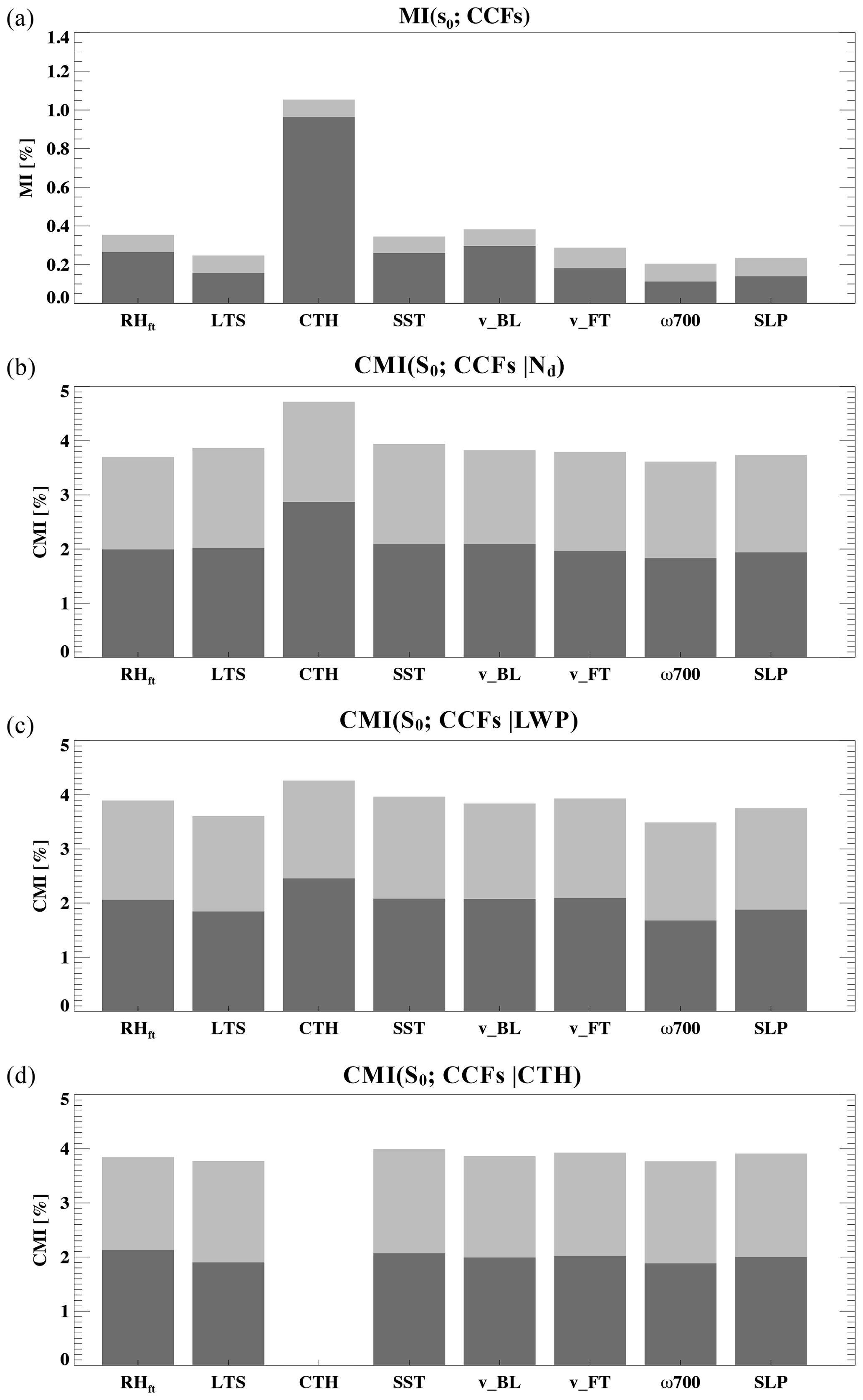
Figure 1 (a) Mutual information (MI; dark gray) for S₀ and eight meteorological factors (MFs; denoted as cloud controlling factors, CCFs), including RH_ft, LTS, CTH, SST, BL, and FT winds, 700 hPa vertical velocity (ω700), and sea level pressure (SLP). (b–d) Conditional MI (CMI; dark gray) for S₀ and the 8 MFs, conditioned by N_d, LWP, and CTH, respectively. Noise-CMI (light gray) is represented by the (conditional) mutual information between MFs and randomly permuted S₀ sample space (effectively noise).

For non-precipitating Sc, LWP decreases with increasing N_d, more markedly when the evaporation–entrainment feedback (EEF; Wang et al., 2003; Xue and Feingold, 2006) becomes more active (right-hand side of the EEF isoline on Fig. 2). The strong EEF process that drives a dramatic decrease in LWP (dln(LWP)$/$dln(N_d) $\sim -\mathrm{0.81}$) leads to a reduction in A_c with increasing N_d until LWP drops below ∼55 g m⁻² (Fig. 2, red circular outlines), after which A_c increases with N_d despite a continuous reduction in LWP, although more than halved in slope (dln(LWP)$/$dln(N_d) $\sim -\mathrm{0.38}$) compared to when LWP is above 55 g m⁻². This increase in A_c with increasing N_d after LWP drops below 55 g m⁻² can be explained by a decrease in entrainment efficiency as LWP decreases (Hoffmann et al., 2020) and an enhanced Twomey effect for less reflective thin clouds (Platnick and Twomey, 1994). The framework for discussion is the commonly used approximation of cloud albedo response to aerosol perturbations (e.g., Bellouin et al., 2020),

$$\begin{array}{}\text{(9)}& S_{\mathrm{0}}={\displaystyle \frac{\mathrm{dln}\left(A_{\mathrm{c}}\right)}{\mathrm{dln}\left(N_{\mathrm{d}}\right)}}={\displaystyle \frac{\mathrm{1}-A_{\mathrm{c}}}{\mathrm{3}}}\left(\mathrm{1}+{\displaystyle \frac{\mathrm{5}}{\mathrm{2}}}{\displaystyle \frac{\mathrm{dln}\left(\mathrm{LWP}\right)}{\mathrm{dln}\left(N_{\mathrm{d}}\right)}}\right),\end{array}$$

in which dln(LWP)$/$dln(N_d) of −0.4 marks the critical value of the LWP adjustment in the entrainment/non-precipitating regime, as it determines the overall sign of the albedo susceptibility approximation, i.e., a warming (negative) or a cooling (positive) effect (e.g., Glassmeier et al., 2021).

The climatological mean-state indicates an overall positive response of A_c to N_d perturbations (a cooling effect), despite an overall negative LWP adjustment (dln(LWP)$/$dln$\left(N_{\mathrm{d}}\right)\sim -\mathrm{0.58}$) that would be sufficient to overcome the Twomey effect and lead to warming, for these relatively high f_c non-precipitating Sc clouds over the NE Pacific region (Fig. 2). The strong and sufficiently negative LWP adjustment derived in this study from long-term satellite observations is in agreement with assessment of Glassmeier et al. (2021) for the same region and regime (a lower bound dln(LWP)$/$dln$\left(N_{\mathrm{d}}\right)=-\mathrm{0.64}$), but based on an ensemble of large-eddy simulations. Such agreement between the results learned from an ensemble of model-simulated time-evolving nocturnal stratocumulus systems and results deduced from a large composite of remote-satellite-sensor-captured afternoon stratocumulus properties might suggest a robustness of these characteristics regarding the relationship between A_c, N_d, and LWP of marine stratocumulus. The result from this work, in addition, points to the importance and necessity of considering the more strongly entraining regime of thicker clouds (LWP > 55 g m⁻²) and the weakly entraining while strongly Twomey–brightening regime of thinner clouds (LWP < 55 g m⁻²) separately; the strength of LWP adjustment is more than halved in the latter ($\sim -\mathrm{0.38}$) compared to the former regime ($\sim -\mathrm{0.81}$), allowing the Twomey effect brightening to prevail.

4.3 Albedo susceptibility and regimes in the LWP–N_d space

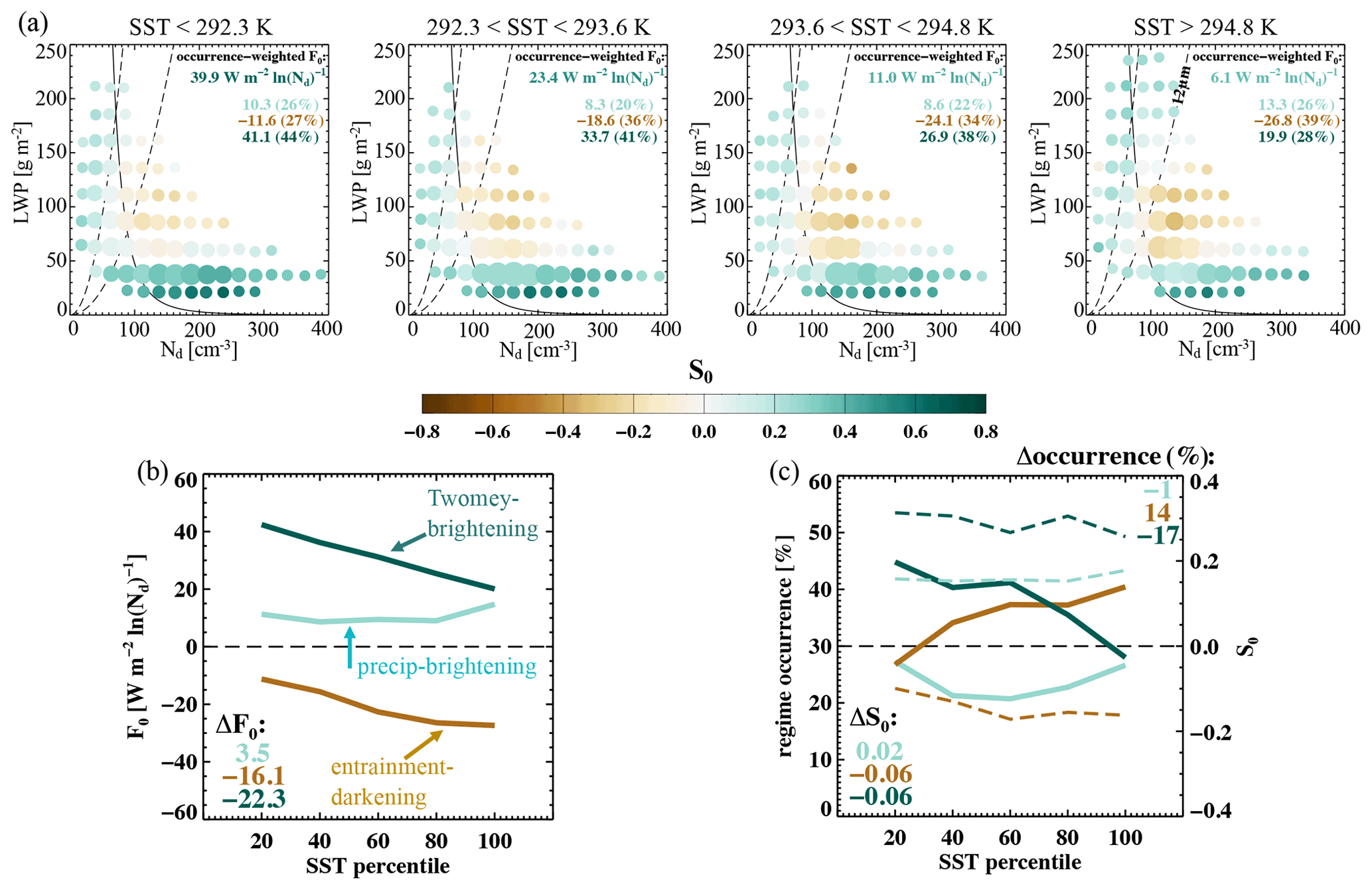
Cloud albedo susceptibility is displayed in LWP–N_d space, with the size of the circles indicating the frequency of occurrence of a particular cloud state (Fig. 3). Precipitating Sc clouds (r_e>12 µm) present an overall cloud brightening potential per N_d perturbation, indicated by the mostly positive susceptibilities, except for some LWP–N_d states that are in the entrainment–evaporation regime (left of the r_e = 12 µm isoline and right of the EEF isoline on Fig. 3). An occurrence-weighted mean radiative susceptibility (F₀) of 10.5±0.91 W m⁻² ln(N_d)⁻¹ corresponding to the precipitating Sc with positive S₀ is consistent with the role of the cloud lifetime effect (Albrecht, 1989, and Fig. 2), such that increases in N_d suppress the warm-rain process, favoring the development of deeper and brighter clouds. This regime is hereafter referred to as the precipitating–brightening regime. It occurs ∼22 % of the time out of all the high-cloud-fraction, single-layer liquid clouds we analyzed over the NE Pacific, based on this 10-year satellite-derived climatology.

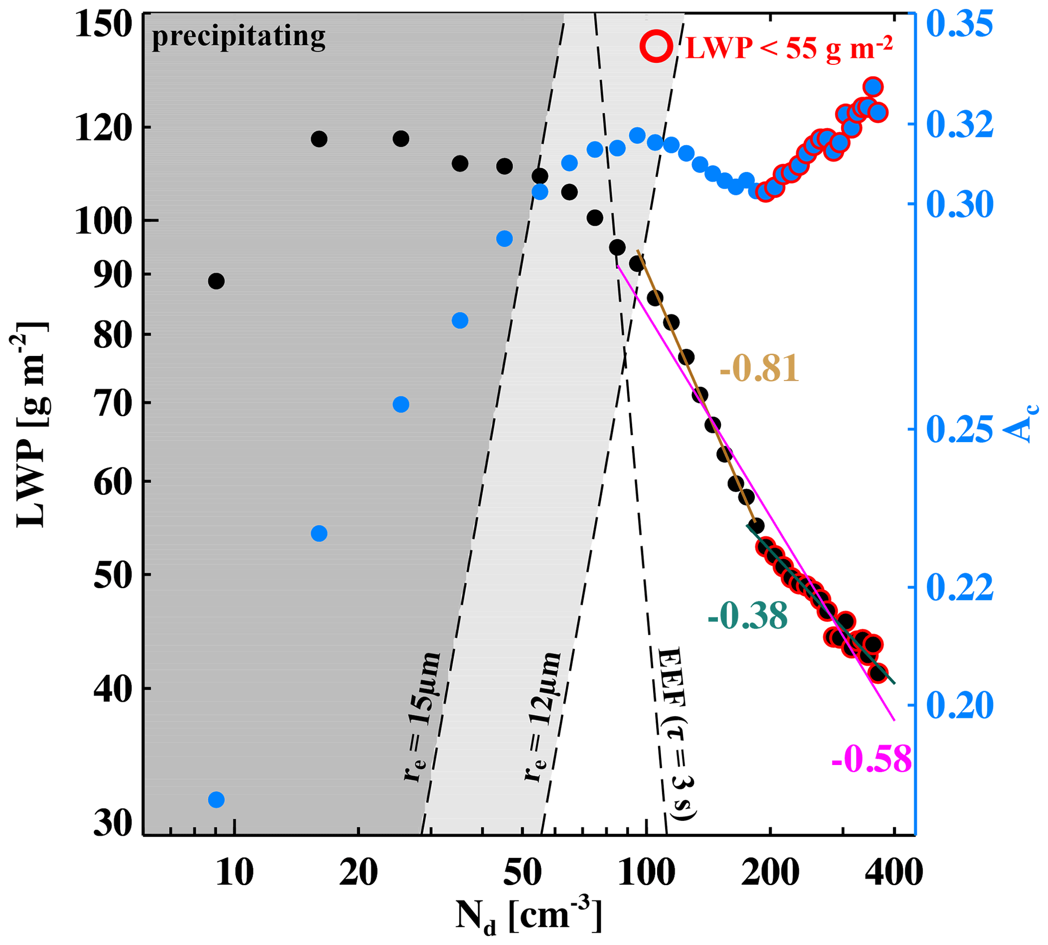
Figure 2 Mean liquid water path (LWP; black dots) and cloud albedo (A_c; blue dots) of each cloud droplet number concentration (N_d) bin (bin size of 10 cm⁻³). Values are shown on logarithm scales. Isolines of evaporation–entrainment feedback (EEF; phase relaxation timescale of 3 s); effective radius (r_e) of 12 and 15 µm (commonly used measures of precipitation) based on an adiabatic condensation rate of 2.14×10⁶ kg m⁻⁴; shades of gray background colors represent a general indicator of likelihood of precipitation; bin-mean LWPs less than 55 g m⁻² are highlighted by red circular outlines. The linear regressed slopes of ln(LWP)–ln(N_d) for all non-precipitating clouds (magenta), non-precipitating clouds with LWP > 55 g m⁻² (brown), and non-precipitating clouds with LWP < 55 g m⁻² (green) are also indicated.

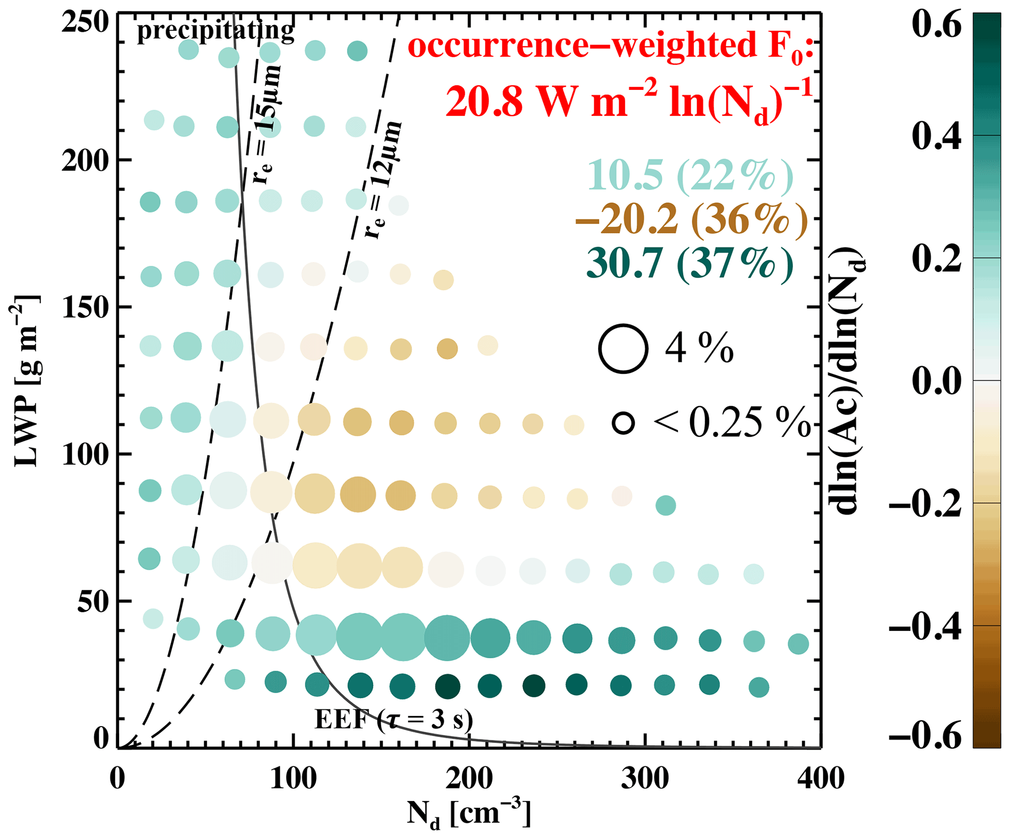
Figure 3 Cloud albedo susceptibility (S₀, colored filled circles) in LWP–N_d space, as bin means (bin size of 25 g m⁻² and 25 cm⁻³). Isolines of r_e of 12 and 15 µm (black dashed) and EEF (as in Fig. 2) are indicated. Size of the filled circles in each panel indicates the relative frequency of occurrence of each bin (reference circle sizes with corresponding occurrence are indicated). Mean radiative susceptibility (F₀) weighted by the frequency of occurrence of each LWP–N_d bin is printed in red (named occurrence-weighted F₀), under which is a decomposition of F₀ into precipitating–brightening (light green; positive susceptibility states with effective radii greater than 12 µm), entrainment–darkening (brown; negative susceptibility states and right-hand side of the EEF isoline), and Twomey–brightening (dark green; non-precipitating states with positive susceptibilities) regimes, with the occurrence of each regime in parentheses.

For non-precipitating Sc, two regimes emerge in the LWP–N_d space, indicated by the changing sign of albedo susceptibility at LWP ≈ 55 g m⁻², with thicker Sc (LWP > 55 g m⁻²) showing a cloud darkening potential (negative S₀) and thinner Sc (LWP < 55 g m⁻²) showing a strong cloud brightening potential (positive S₀) per N_d perturbation (Fig. 3). This is consistent with the inverted V-shape dependence of mean-state A_c as a function of N_d for non-precipitating Sc shown in Fig. 2 (blue dots), with the turning point being around 55 g m⁻². As discussed in Sect. 4.2, the non-precipitating cloud states with negative S₀ are dominated by the entrainment-driven LWP adjustment ($\sim -\mathrm{0.81}$, Fig. 2, brown fitting line), which is double the critical slope value (−0.4) for entering the warming regime (Glassmeier et al., 2021). This entrainment–evaporation regime cloud state (right of the EEF isoline on Fig. 3) with negative S₀ occurs ∼36 % of the time out of the cloudy scenes we analyzed. It produces an occurrence-weighted $F_{\mathrm{0}}=-\mathrm{20.2}\pm \mathrm{1.89}$ W m⁻² ln(N_d)⁻¹ and is hereafter referred to as the entrainment–darkening regime (mostly non-precipitating).

The thinner Sc (LWP < 55 g m⁻²) not only possess strong positive albedo susceptibilities for reasons discussed in Sect. 4.2, but these cloud states also occur the most frequently (∼37 % of the time; Fig. 3). As a result, a dominating positive occurrence-weighted mean F₀ of 30.7±1.60 W m⁻² ln(N_d)⁻¹ is associated with these non-precipitating cloud states with positive S₀, hereafter referred to as the Twomey–brightening (non-precipitating) regime. Climatologically, the cloud-state-dependent albedo susceptibilities and their corresponding frequency of occurrence together determine that the stratocumulus deck over the NE Pacific presents an overall cloud brightening potential with an occurrence-weighted F₀ of 20.8±0.96 W m⁻² ln(N_d)⁻¹ (Fig. 3), in agreement with the results shown in Fig. 2.

5 Meteorological constraints

One of the main questions we want to address is under what meteorological conditions are marine low clouds most/least susceptible to aerosol perturbations or, in other words, what is the influence of meteorology on albedo and radiative susceptibilities? Then, by quantifying the frequency of occurrence of susceptible conditions, and the potential radiative effect associated therewith, we have the means to quantify the radiative effect of aerosol–cloud interactions. In this section, we assess meteorological constraints on low-cloud albedo susceptibility from multiple perspectives, with a focus on the covariability among meteorological drivers: where to find susceptible and less susceptible conditions in meteorological factor spaces (Sect. 5.1), the role of seasonal covariability in meteorological conditions (Sect. 5.2), and the impact of individual meteorological factors on the occurrence of susceptibility regimes and the overall occurrence-weighted radiative susceptibility (Sect. 5.3).

5.1 Albedo susceptibility in meteorology spaces

We map cloud states in the LWP–N_d space (Fig. 3) directly onto meteorological spaces (Fig. 4) to reveal the association between meteorological conditions and the radiative susceptibility regimes identified in Sect. 4.2. A clear separation of the entrainment–darkening and Twomey–brightening regimes is evident in all six meteorological spaces (Fig. 4, brown and green/blue open circles), more markedly in the direction of cloud-top height (Fig. 4a–c). Moreover, these two regimes tend to cluster in meteorological spaces: the Twomey–brightening regime clusters at low CTH, highest LTS, relatively low SST, and lowest RH_ft, and the entrainment–darkening regime clusters at higher CTH, lower LTS, higher SST, and higher RH_ft, compared to the Twomey–brightening regime (Fig. 4). The clustering of these two regimes in these meteorological spaces is consistent with their states in the LWP–N_d space, as stratocumulus clouds with higher cloud tops usually have higher LWP over the NE Pacific region. Therefore, thicker and deeper clouds are more strongly affected by the cloud-top entrainment feedbacks, leading to decreases in LWP as N_d increases, whereas thinner and lower Sc are subject to less effective entrainment processes, maintaining the cloud LWP such that an increase in N_d can sufficiently decrease r_e and brighten the clouds. The vertical extent of the subtropical marine stratocumulus or the depth of the stratocumulus-topped boundary layer (STBL) is controlled, to first order, by the LTS at longer timescales (Eastman et al., 2017) and RH_ft at shorter timescales (Eastman et al., 2017; Eastman and Wood, 2018), such that enhanced LTS (a stronger buoyancy gradient across the inversion) or higher free-tropospheric humidity (less radiative and evaporative cooling), all else being equal, limits the entrainment of free-tropospheric air and thereby suppresses the deepening of marine boundary layers. Hence, the primary occurrence of the Twomey–brightening regime is under the highest LTS conditions but, perhaps counterintuitively, also under the lowest RH_ft conditions (Fig. 4b, e, and f). This is because large-scale meteorological conditions are strongly correlated over eastern subtropical oceans where the Earth's major marine stratocumulus decks are formed (Wood, 2012), such that LTS and RH_ft are negatively correlated (evident in Fig. 4e and further discussed in 4.3.3), as prevailing free-tropospheric subsidence transports dry upper-level air downward and increases the stability.

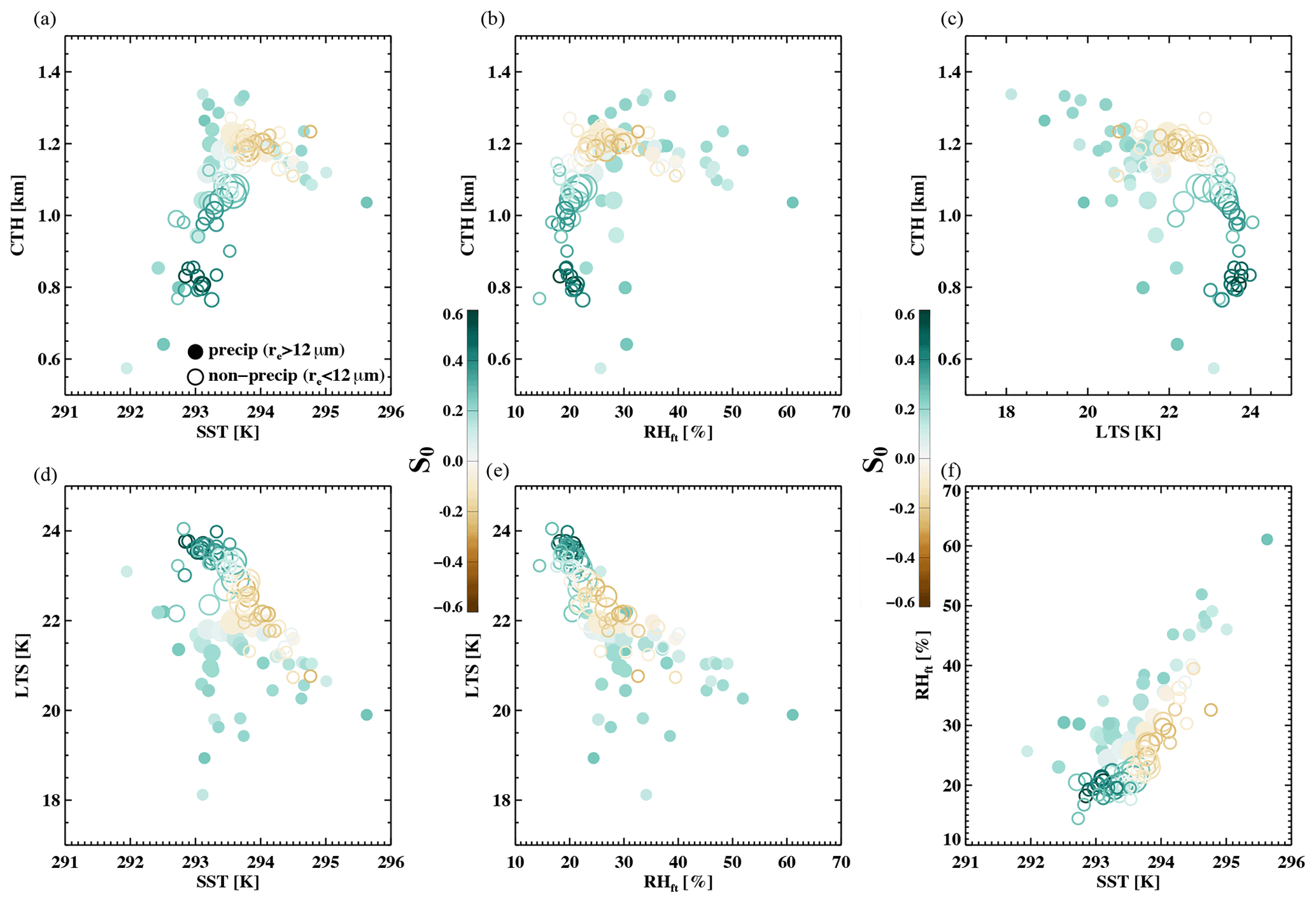
Figure 4 Mean meteorological/cloud state conditions associated with each LWP–N_d bin in Fig. 3, in the space of (a) CTH–SST, (b) CTH–RH_ft, (c) CTH–LTS, (d) LTS–SST, (e) LTS–RH_ft, and (f) RH_ft–SST. Size and color of the circles represent the frequency of occurrence and the mean S₀ of that LWP–N_d bin, respectively, as shown in Fig. 3. Precipitating clouds (based on a r_e threshold of 12 µm) and non-precipitating clouds are indicated by filled and open circles, respectively.

In contrast, the precipitating–brightening regime tends to spread out in the meteorological spaces, overlapping with the other two regimes, except in the spaces of RH_ft and LTS (e.g., Fig. 4e). This suggests precipitation-suppression-driven cloud brightening tends to occur, first, when LTS is weak (less than 21 K), regardless of RH_ft or SST; and, second, when the free troposphere is the moistest (>45 %), co-occurring with the highest SST conditions (>294.5 K) (Fig. 4f). Despite high-SST conditions, the precipitating–brightening branch appears under high RH_ft, indicating a dominant role of the free-tropospheric humidity. Here, enhanced free-tropospheric humidity (a reduced humidity gradient across the cloud top) slows/weakens droplet evaporation, creating favorable conditions for precipitation, which is susceptible to aerosol-induced warm-rain suppression process and thereby cloud brightening. This role of RH_ft is reinforced by the fact that the precipitating–brightening branch is displaced from the non-precipitating branch in Fig. 4f, where RH_ft alone determines which susceptibility regimes the clouds will be in at a constant SST.

The fact that two of the susceptibility regimes cluster while the other spreads out in the meteorological spaces serves to expand our discussion on the concept of equifinality. We previously discussed that different meteorological conditions may produce the same cloud state (LWP, N_d). Here we see that different meteorological conditions may produce the same S₀. This ties back to the importance of understanding and quantifying the covariabilities between meteorological factors, as multiple environmental factors may be needed to explain all the variability in cloud states (e.g., Chen et al., 2021) and thereby albedo susceptibility.

5.2 The role of seasonal covariability in meteorological conditions

Monthly climatologies of ERA5 meteorological factors, including LTS, SST, RH_ft, and 700 hPa subsidence, averaged over the NE Pacific show a strong seasonality and a tight correlation among these factors (Fig. 5a). The annual cycle in SST (blue) and 700 hPa vertical velocity (gray) are correlated and anti-correlated with that of the Northern Hemispheric insolation, respectively (not shown), such that summer time (June–September) SST is the highest, whereas free-tropospheric subsidence is the weakest due to a weakened Hadley circulation when insolation is at its annual maximum in the Northern Hemisphere. Moreover, the annual cycle in free-tropospheric humidity (black) is very well anti-correlated with that of the free-tropospheric subsidence, leading to a positive (although lagged) correlation between RH_ft and SST (also evident in Fig. 4f). As the Hadley circulation starts to strengthen in January, indicated by the enhancing 700 hPa subsidence (January to May), and SST over the subtropical ocean remains cool during boreal spring, LTS (red) increases markedly. SST starts to increase as the Northern Hemisphere enters its summer season, resulting in a weakening of the Hadley circulation and the free-tropospheric subsidence and leading to a continuous decrease in LTS from June until January. As a result, LTS peaks in June, leading the annual maximum in SST by 3 months (Fig. 5a).

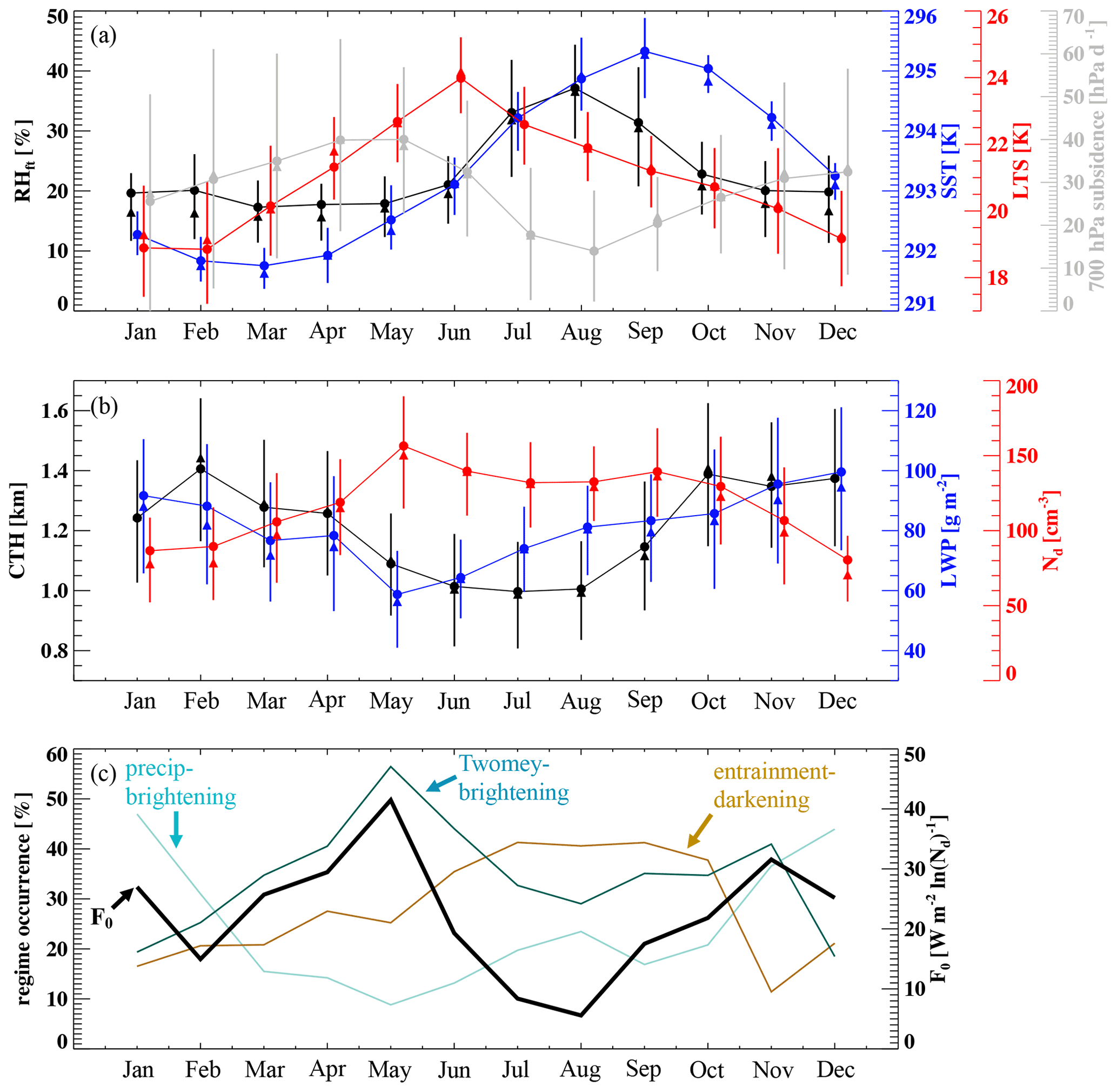
Figure 5 Annual cycle of (a) ERA5 RH_ft (black), SST (blue), LTS (red), 700 hPa subsidence (gray), (b) MODIS CTH (black), LWP (blue), and N_d (red), as monthly means (filled circles), medians (filled triangles), and interquartile ranges (vertical bars). (c) Annual cycle of occurrence-weighted F₀ (black) and the occurrence of each albedo susceptibility regime (colored).

In response to the strengthening LTS during boreal spring, both CTH (black) and cloud LWP (blue) decrease, with cloud LWP reaching its annual minimum in May (Fig. 5b). The thinnest clouds of the year give rise to the annual maximum in the occurrence of the Twomey–brightening regime in May, resulting in an annual maximum of F₀ (Fig. 5c). As LTS decreases and SST continues to warm during boreal summer and fall, cloud LWP and CTH increase until December, when LTS is at its annual minimum and the precipitating–brightening regime is at its annual maximum occurrence, resulting in a secondary peak in the annual cycle of F₀. During the boreal summer months (June–September), when SST is the highest, the entrainment–darkening regime is at its annual maximum occurrence, resulting in the lowest F₀ throughout the annual cycle. The high summertime N_d also favors the occurrence of the entrainment–darkening regime through the entrainment feedbacks. This is in agreement with the finding that warmer SST over the northeast (NE) Atlantic leads to mostly darkening clouds (Zhou et al., 2021). Although F₀ responds to SST over the NE Pacific the same way as it does over the NE Atlantic, marine low clouds over the NE Pacific never enter an overall darkening regime, likely due to the co-occurring high free-tropospheric humidity and high-SST conditions and thereby a relatively persistent and high occurrence of the precipitating–brightening regime (July–September), which is rarely the case for the high-SST conditions over the NE Atlantic in Zhou et al. (2021).

5.3 Meteorology affects the occurrence of albedo susceptibility regimes

As discussed in Sect. 4.1, meteorological or environmental conditions influence the albedo susceptibility of a cloud field to aerosol perturbations through regulating the state of the clouds, e.g., N_d, LWP. Because individual meteorological factors tend to covary with others, we modify the traditional approach of binning results by individual meteorological factors. Instead we bin by a single meteorological factor and allow all others to covary. We present albedo susceptibilities in LWP–N_d space as a function of individual meteorological factors (Figs. 6–9), with a focus on the impact of meteorology on the occurrence and the strength of each albedo susceptibility regime.

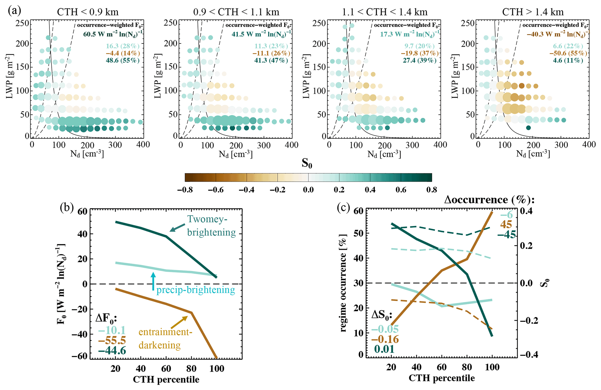
Figure 6 (a) As in Fig. 3 but conditioned on cloud-top height (CTH) quartiles. Occurrence-weighted mean (b) F₀ and (c) regime-mean S₀ (dashed curves) and regime–occurrence (solid curves) of the three albedo susceptibility regimes (defined in Fig. 3) as a function of CTH; increment of 20th percentile.

Figure 7 As in Fig. 6 but for lower-tropospheric stability (LTS).

Figure 8 As in Fig. 6 but for free-tropospheric relative humidity (RH_ft).

Figure 9 As in Fig. 6 but for sea surface temperature (SST).

5.3.1 Cloud-top height (CTH)

As cloud-top heights of marine Sc increase or as the Sc-topped boundary layers deepen, clouds are more likely to develop higher LWPs and are more likely to precipitate. A pronounced decrease in occurrence-weighted radiative susceptibility with increasing CTH, from 60.5 W m⁻² ln(N_d)⁻¹ to −40.3 W m⁻² ln(N_d)⁻¹, is noted (Fig. 6a). The F₀ uncertainties in this section are reported in Tables S1–S4 in the Supplement. The remarkable decrease in F₀ can be reasoned through two contributing mechanisms, (i) changes in the magnitude of S₀ and (ii) a shift in the frequency of occurrence of cloud states (LWP, N_d), as cloud top elevates. First, regarding changes in the magnitude of S₀, a clear enhancement in the negative susceptibilities in the entrainment–darkening regime, by −0.16, is evident as CTH increases (Fig. 6a and dashed curves in 6c), consistent with an increasing influence of the entrainment feedbacks as cloud deepens. For the precipitating–brightening Sc, S₀ decreases slightly with increasing CTH, by −0.05, leading to a steady decrease in regime-mean F₀, by −10.1 W m⁻² ln(N_d)⁻¹ (Fig. 6b), given little change in the occurrence of the regime. This could reflect two possible balancing mechanisms: (i) a balance between warm-rain suppression and the increasing precipitation (droplet removal) efficiency with deeper/higher clouds; (ii) a balance between warm-rain suppression and the strengthening entrainment drying with higher cloud tops.

Second, a pronounced shift in the occurrence of the albedo susceptibility regimes (Fig. 6a and solid curves in 6c) is perhaps more evident, such that the marine Sc clouds over the NE Pacific are more likely to be found in the entrainment–darkening regime (55 %) rather than the Twomey–brightening regime (11 %) in the highest CTH quartile. This is in contrast to the lowest CTH quartile, where the Twomey–brightening regime (55 %) is much more likely to occur than the entrainment–darkening regime (14 %). This shift in regime occurrence (and the MFs that define them) as CTH increases is the primary driver of the significant changes in the overall occurrence-weighted F₀, in which the contribution from the Twomey–brightening regime shrinks by 44.6 W m⁻² ln(N_d)⁻¹ and the contribution from the entrainment–darkening regime increases by 55.5 W m⁻² ln(N_d)⁻¹ (Fig. 6b). In a nut shell, stronger entrainment and more entrainment drying are expected for clouds with higher cloud tops.

5.3.2 Lower-tropospheric stability (LTS)

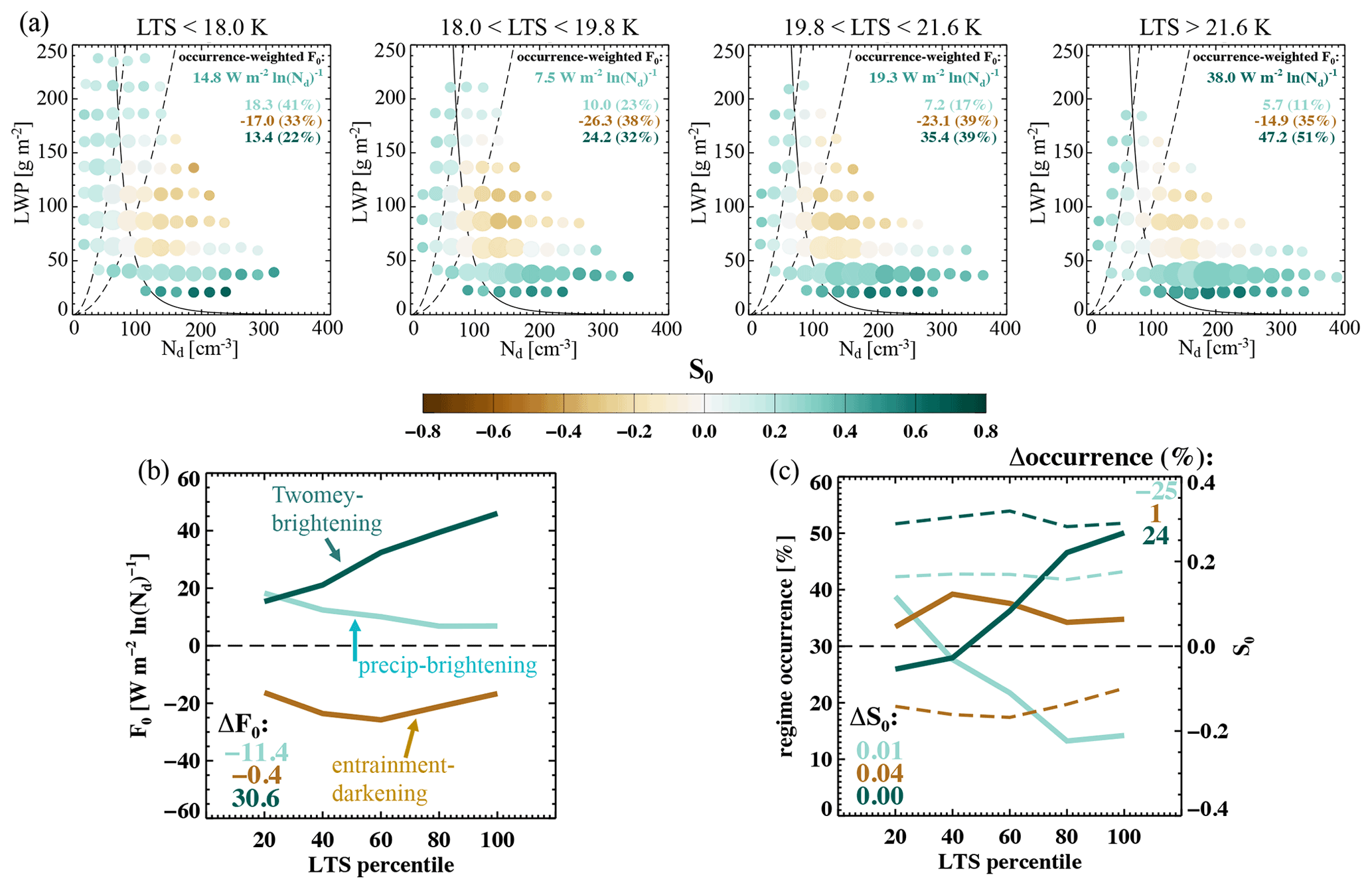
When lower-troposphere stability is low (unstable conditions, leftmost panel on Fig. 7a), clouds are most frequently observed in high-LWP states, consisting of the most frequently occurring precipitating–brightening regime (41 % of the time) whose radiative susceptibility contribution is almost entirely offset by that of the less frequently occurring entrainment–darkening regime (33 % of the time). This is consistent with the governing role of LTS on stratocumulus-topped marine boundary layer characteristics, such that weaker LTS allows stronger entrainment of free-tropospheric air into the boundary layer, resulting in on-average deeper boundary layers and thicker clouds. As LTS increases, the precipitating–brightening regime occurs less and less frequently (from 41 % to 11 %), whereas the occurrence of the Twomey–brightening regime increases from 22 % to 51 % (Fig. 7a), as expected from the suppressing effect of high atmospheric stability on the deepening of STBL.

The impact of LTS on cloud-top entrainment can be directly seen by comparing the strength (darkness of the color) and the weighted F₀ contribution (labeled) of the entrainment–darkening regime across LTS quartiles (Fig. 7a). However, one should be mindful of the obscuring effect of the covarying RH_ft: when LTS is low, RH_ft is high (discussed in Sect. 5.1 and shown in Fig. 4e), which suppresses the enhanced entrainment drying that would have occurred if the free troposphere above were dry. Nevertheless, the entrainment–darkening regime is weakest under the highest LTS condition (rightmost panel on Fig. 7a), compared to the other LTS quartiles. However, the lowest LTS quartile does not exhibit the strongest entrainment–darkening regime, owing to the co-occurring high-RH_ft conditions.

In a nutshell, increasing LTS mostly affects the occurrence of the precipitating–brightening regime (by −25 %) and the Twomey–brightening regime (by +24 %) (Fig. 7c), leading to changes in the occurrence-weighted F₀ of −11.4 and +30.6 W m⁻² ln(N_d)⁻¹, respectively (Fig. 7b).

5.3.3 Free-tropospheric humidity (RH_ft)

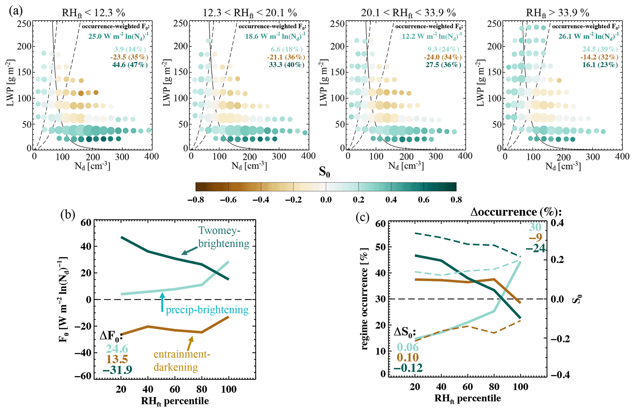
The effect of RH_ft on radiative susceptibility has two aspects. First, moister air above cloud top reduces the humidity gradient across the cloud-top inversion, thereby weakening the evaporation–entrainment feedback. This is evident in comparisons between the leftmost and rightmost panels on Fig. 8a, where fewer cloud states in LWP–N_d space are represented by a weakened entrainment–darkening regime under higher-RH_ft conditions, consistent with the findings in Ackerman et al. (2004) and Chen et al. (2014). Second, as conditions in the free troposphere become more humid with decreasing atmospheric stability (negatively correlated LTS and RH_ft), marine low-level clouds are more likely to possess higher LWP and reside in a more favorable environment for precipitation, indicated by the high occurrence of the precipitating–brightening regime (39 %) in the highest RH_ft quartile (also consistent with Ackerman et al., 2004). ERA5 humidity profiles also indicate a positive correlation between RH_ft and the RH within the boundary layer (not shown), further supporting higher LWP. The increase in LWP with increasing RH_ft leads to a shift in cloud state away from the Twomey–brightening regime towards the other two regimes but mostly towards the precipitating–brightening regime (Fig. 8a). Worth noting is that the magnitude of these two effects of RH_ft on albedo susceptibility and their occurrence amplify as RH_ft increases: note the steep changes at the highest 20th percentile of RH_ft in Fig. 8b–c.

The Twomey–brightening and the precipitating–brightening regimes are more sensitive (manifested more in their frequency of occurrence rather than their strength) to variations in RH_ft and LTS (Figs. 7–8), whereas the sensitivity of the entrainment–darkening regime to these two factors is largely suppressed by the negative correlation between large-scale RH_ft and LTS conditions over this region. This again points to the important role of covarying meteorological conditions in affecting albedo susceptibility.

5.3.4 Sea surface temperature (SST)

As sea surface temperature increases over the NE Pacific, radiative susceptibility decreases from 39.9 to 6.1 W m⁻² ln(N_d)⁻¹ (Fig. 9a). First, SST changes are the driver of changes in many other meteorological factors, e.g., surface fluxes, marine boundary layer height, LTS, and humidity. Here, we do not attempt to separate out the role of SST on radiative susceptibilities while controlling for other MFs but rather explore the radiative susceptibility as a function of SST, with all the inherent covariability between SST and other MFs. In general, cloud states shift towards higher LWP and lower N_d, an indication of thicker clouds with larger droplet sizes, as SST increases, suggesting a higher likelihood of precipitation and scavenging for the clouds in the warmer SST conditions (more circles to the left of the 12 µm isoline on Fig. 9a, rightmost panel). This is consistent with an increase in SST leading to an increase in surface fluxes and a weaker LTS in a well-mixed marine boundary layer, both supporting the development of deeper Sc with higher LWPs (similar to the response of trade-wind cumulus to warming in Vogel et al., 2016). Another effect associated with thicker clouds is the creation of favorable conditions for the entrainment feedbacks, which is shown as a strengthening of the entrainment–darkening S₀ (Fig. 9a, brown circles getting darker). As a result, as SST increases, the increasing occurrence of the strengthening entrainment–darkening regime and the decreasing occurrence of the Twomey–brightening regime (Fig. 9c) lead to the overall decrease in F₀, by ∼ 34 W m⁻² ln(N_d)⁻¹ (Fig. 9a, leftmost vs rightmost).

In the current climate, the free-tropospheric humidity over the NE Pacific correlates well with SST through the seasonality in large-scale circulation (i.e., the free-tropospheric subsidence related to the Hadley circulation), such that higher SST is associated with enhanced above-cloud humidity, favoring the occurrence of the precipitating–brightening regime (Fig. 9c, the U-shaped occurrence variation of the precipitating–brightening regime). The rebounding of the precipitating–brightening regime at high SST (Fig. 9b and c) partially offsets the darkening potential that would otherwise dominate the overall radiative susceptibility, leading to a warming effect, in the absence of the enhanced free-tropospheric humidity (similar to over the NE Atlantic; Zhou et al., 2021). However, if SST continues to rise in the coming decades, and assuming the same trend observed in Fig. 9, we might expect the NE Pacific stratocumulus region to exhibit an overall darkening potential to aerosol perturbations.

In the assessment of the role of individual MFs, it is important to emphasize that a change in one MF is usually associated with changes in other MFs (with the seasonal covariability in meteorological conditions as an example). Our goal in this section has been to retain this covariability between MFs in our analyses, with the aim of quantifying influences of meteorology on radiative susceptibility in the manner in which nature is observed. In selecting one variable for stratification and allowing all others to covary, we come closer to reality than traditional investigations of individual MFs in which all others are held constant. The latter approach only represents a small portion of the natural variability, and the role of covariabilities between MFs is missed.

6 Concluding remarks

This study quantifies the albedo susceptibility and radiative susceptibility to N_d perturbations of high-f_c, single-layer marine low clouds over the NE Pacific stratocumulus region, using 10 years of MODIS-retrieved daytime cloud properties and CERES-measured radiative fluxes at the top of the atmosphere. A novel aspect of this study is the assessment of susceptibility across a LWP–N_d space, such that albedo susceptibility associated with individual cloud states (LWP, N_d) and, more importantly, their frequencies of occurrence are quantified. Moreover, the effects of ERA5 meteorological factors and their covariability, on the albedo susceptibility are explored. This allows us to quantify conditions under which low clouds are most/least susceptible to aerosol perturbations and how frequently these conditions occur. Robust establishment of three albedo susceptibility regimes is found regardless of meteorological states or environmental conditions; however, the occurrence and strength of these regimes are clearly modified by meteorological conditions. The key findings are the following.

1. Based on mutual information analysis, LWP, N_d, and CTH are shown to be the governing factors of low-cloud albedo susceptibility. Individual meteorological factors add very little (less than a percent) shared information with S₀ if the aforementioned three variables are known (Fig. 1). That said, meteorological factors are shown to affect the overall radiative susceptibility of marine Sc but mainly through governing the frequency of occurrence of cloud states, i.e., LWP and N_d, and thereby the occurrence of each of the susceptibility regimes (Figs. 6–9). This led us to use LWP–N_d as our parameter space, in which we further explore albedo susceptibilities and the brightening versus darkening regimes.

2. From a climatological mean-state perspective, LWP and N_d are negatively correlated for non-precipitating Sc (Fig. 2), consistent with previous polar-orbiting satellite-based studies (e.g., Gryspeerdt et al., 2019a; Possner et al., 2020). Results from the current study, however, indicate that despite the negative LWP adjustment, cloud albedo increases with increasing N_d for non-precipitating Sc overall, pointing to the importance of considering the high-LWP cloud states separately from the low-LWP cloud states, as the negative LWP adjustments are clearly different for thicker versus thinner Sc (Fig. 2).

3. When cloud albedo susceptibility is mapped onto the LWP–N_d state space, three susceptibility regimes emerge: (i) the Twomey–brightening regime (occurring 37 % of the time, contributing 30.7 ± 1.55 W m⁻² ln(N_d)⁻¹), consisting of non-precipitating thinner clouds (LWP $<\sim \mathrm{55}$ g m⁻²) and consistent with a dominating Twomey effect for clouds of relatively low albedo and weaker entrainment; (ii) the entrainment–darkening regime (occurring 36 % of the time, contributing $-\mathrm{20.2}\pm \mathrm{1.86}$ W m⁻² ln(N_d)⁻¹), comprising mostly non-precipitating thicker clouds (LWP $>\sim \mathrm{55}$ g m⁻²) and consistent with entrainment feedbacks that drive a decrease in LWP with increasing N_d; (iii) the precipitating–brightening regime (occurring 22 % of the time, contributing 10.5±1.45 W m⁻² ln(N_d)⁻¹), comprising precipitating clouds with effective radii mostly greater than 12 µm and consistent with the cloud lifetime effect due to a suppressed warm-rain process (Fig. 3). An overall cloud brightening potential of 20.8±0.96 W m⁻² ln(N_d)⁻¹ is found for the marine low clouds over the NE Pacific stratocumulus region, after the frequency of occurrence of each regime is accounted for.

4. When cloud states, along with their associated radiative susceptibilities, are mapped to meteorological spaces of LTS, SST, CTH, and RH_ft, the entrainment–darkening regime and the Twomey–brightening regime are clearly associated with distinct meteorological conditions. The Twomey–brightening regime occurs most frequently under low CTH, highest LTS, low SST, and lowest RH_ft conditions. Such a combination of these meteorological factors occurs in May as a result of the seasonally covarying meteorological conditions related to the large-scale circulation over the NE Pacific. The entrainment–darkening regime occurs most frequently under relatively high CTH and intermediate LTS, SST, and RH_ft conditions, which prevail during the boreal summer months (July–September). The precipitating–brightening regime mostly manifests in unstable conditions (low LTS), occurring during winter months (November–January), but a very moist free troposphere (co-occurring with high SST in August) also promotes the occurrence of this regime (Figs. 4–5).

5. As cloud-top height or marine boundary layer height increases, cloud states shift towards larger LWP, resulting in a pronounced decrease in the Twomey–brightening regime occurrence and a marked increase in the occurrence of the entrainment–darkening regime. This is accompanied by an enhanced entrainment–darkening susceptibility strength and a reduced precipitating–brightening susceptibility strength. As a result, F₀ decreases substantially with increasing CTH, from 60 to −40 W m⁻² ln(N_d)⁻¹ (Fig. 6).

6. The influence of LTS on F₀ is mainly exerted via the frequency of occurrence of each susceptibility regime rather than its mean S₀. Strong stability (high LTS) leads to shallower Sc that mostly occur in the Twomey–brightening regime, whereas unstable conditions (low LTS) allow clouds to grow deeper and become more prone to precipitation, leading to high occurrence of the precipitating–brightening regime (Fig. 7).

7. A moist free troposphere has two major impacts on the radiative susceptibility: (i) a reduced humidity gradient across the cloud-top inversion weakens the evaporation–entrainment process, leading to a less negative LWP adjustment for thicker non-precipitating clouds; (ii) a moist free troposphere, co-occurring with low LTS, gives rise to a higher occurrence of thicker and deeper clouds, driving a major shift of cloud states away from the Twomey–brightening regime, mostly into the precipitating–brightening regime (Fig. 8).

8. The negative correlation between large-scale LTS and RH_ft conditions obscures their individual role in affecting the cloud-top entrainment–evaporation process (Figs. 7–8).

9. Increases in SST lead to a deeper marine boundary layer, lower LTS, and thicker clouds. As a result, F₀ decreases with increasing SST, owing to a higher occurrence of deeper clouds (meaning less occurrence of the Twomey–brightening regime) and a stronger entrainment–darkening regime associated with the weakened stability. In contrast to the NE Atlantic (Zhou et al., 2021), moist free-tropospheric conditions, co-occurring with high SSTs, during summertime over the NE Pacific, hamper the role of the strengthening entrainment–darkening regime, by shifting clouds towards the precipitating–brightening regime (Fig. 9).

By focusing on this marine stratocumulus-dominated region/regime over the NE Pacific, we were able to separate cloud states into three clearly defined susceptibility regimes in the LWP–N_d space and link the responses to existing understanding of marine stratocumulus. Future work quantifying the occurrence and strength of these three regimes at various oceanic locations, associated with different meteorological regimes/conditions, will enable an extended satellite-based assessment of the radiative susceptibility of global marine low clouds. Moreover, if aerosol perturbations, natural or anthropogenic, are estimated in some form, the characterization and quantification of radiative susceptibility regimes provided in this study can be used to provide a global estimate of radiative forcing or radiative effect, due to aerosol-marine low-cloud interactions. Such assessments are planned for a follow-on study.