Impacts of active satellite sensors' low-level cloud detection limitations on cloud radiative forcing in the Arctic

Previous studies revealed that satellites sensors with the best detection capability identify 25 %–40 % and 0 %–25 % fewer clouds below 0.5 and between 0.5–1.0 km, respectively, over the Arctic. Quantifying the impacts of cloud detection limitations on the radiation flux are critical especially over the Arctic Ocean considering the dramatic changes in Arctic sea ice. In this study, the proxies of the space-based radar, CloudSat, and lidar, CALIPSO (Cloud-Aerosol Lidar and Infrared Pathfinder Satellite Observations), cloud masks are derived based on simulated radar reflectivity with QuickBeam and cloud optical thickness using retrieved cloud properties from surface-based radar and lidar during the Surface Heat Budget of the Arctic Ocean (SHEBA) experiment. Limitations in low-level cloud detection by the space-based active sensors, and the impact of these limitations on the radiation fluxes at the surface and the top of the atmosphere (TOA), are estimated with radiative transfer model Streamer. The results show that the combined CloudSat and CALIPSO product generally detects all clouds above 1 km, while detecting 25 % (9 %) fewer in absolute values below 600 m (600 m to 1 km) than surface observations. These detection limitations lead to uncertainties in the monthly mean cloud radiative forcing (CRF), with maximum absolute monthly mean values of 2.5 and 3.4 Wm⁻² at the surface and TOA, respectively. Cloud information from only CALIPSO or CloudSat lead to larger cloud detection differences compared to the surface observations and larger CRF uncertainties with absolute monthly means larger than 10.0 Wm⁻² at the surface and TOA. The uncertainties for individual cases are larger – up to 30 Wm⁻². These uncertainties need to be considered when radiation flux products from CloudSat and CALIPSO are used in climate and weather studies.

1 Introduction

Clouds are an important modulator of radiation flux at the surface and top of the atmosphere (TOA). Major advances in understanding cloud processes in the climate system have been made, and the amount of uncertainty in cloud feedback has decreased by 50 % in recent years, as reported in the technical summary of the sixth assessment report of the Intergovernmental Panel on Climate Change (Arias et al., 2021). However, cloud feedback still has the largest uncertainty among all climate feedback types (Arias et al., 2021). Climate prediction relies on a deepened understanding of clouds in the current climate system and how they evolve in the future. Arctic clouds are unique for being ubiquitous at low altitudes within and above a stable boundary layer and for persistent mixed-phase stratiform clouds in the boundary layer (Shupe et al., 2006; Cesana et al., 2012). Cloud properties and cloud formation, maintenance, and dissipation mechanisms in the Arctic stand out because of the unique environment in the Arctic, e.g., extremely low temperatures, ubiquitous surface-based temperature and moisture inversions, and very limited local sources of cloud condensation nuclei and ice nuclei. The harsh environment in the Arctic makes in situ observations of Arctic clouds challenging. Coupled with the dramatic changes in the Arctic, especially the Arctic sea ice in the last few decades, Arctic clouds may pose the largest challenge in improving our understanding of cloud feedback mechanisms (Vavrus et al., 2009; Tan and Storelvmo, 2019; Arias et al., 2021).

Better understanding of Arctic clouds requires accurate observations/measurements of three-dimensional cloud macrophysical and microphysical properties. Observations from surface-based instruments and space-based passive and active sensors have been used to study Arctic cloud properties and their climatology and interannual variabilities. These observations have their relative strengths and limitations. Surface observations with active lidar and radar have a superior capability to measure cloud properties of the whole column (Shupe et al., 2011; Shupe, 2011; Zhao and Wang, 2010; Dong et al., 2010) and to resolve the diurnal cycle but with poor spatial coverage. Cloud products from passive satellite sensors in the visible and infrared spectrum, e.g., AVHRR, MODIS, and VIIRS, have good spatial coverage and a long time series, which is critical for climate studies (Key et al., 2016). However, such data sets are limited in providing whole cloud vertical distributions due to signal saturation and have difficulties in detecting all clouds in the polar regions, especially at night (Liu et al., 2010). Observations from space-based active radar and lidar with other sensors potentially provide three-dimensional cloud properties (Stephens et al., 2002; Winker et al., 2009; Vaughan et al., 2009; Hunt et al., 2009; Turner, 2005; Zuidema et al., 2005); these products have been used to study global cloud spatial distributions and their temporal changes (Li et al., 2015; Naud et al., 2015; Devasthale et al., 2011; Huang et al., 2012; Mace et al., 2009; Mace and Zhang, 2014; Sassen and Wang, 2008, 2012; Liu et al., 2012a), along with longwave and shortwave radiation flux profiles and the corresponding heating rates (L'Ecuyer et al., 2008; Henderson et al., 2013). In addition to their relatively limited spatial coverage compared to passive satellite sensors, space-based radar, e.g., CloudSat, has issues with radar ground clutter, while space-based lidar, e.g., the Cloud-Aerosol Lidar with Orthogonal Polarization (CALIOP) aboard the Cloud-Aerosol Lidar and Infrared Pathfinder Satellite Observations (CALIPSO), has signal attenuation issues from the clouds above the low-level clouds (Marchand et al., 2008; Winker et al., 2009; Blanchard et al., 2014; Liu et al., 2017; Christensen et al., 2013), both of which lead to detection limitations of clouds near the surface. Even the state-of-art combined satellite-based radar and lidar do not detect all low-level clouds (Blanchard et al., 2014; Liu et al., 2017).

Over land in the Arctic, with colocated observations of cloud properties from surface-based radar and lidar as reference/truth and from satellite-based radar and lidar (CloudSat and CALIPSO), a few previous studies have shown that satellite-based radar and lidar detect slightly more clouds 2 km above mean sea level (a.m.s.l.), comparable cloud amounts between 1 and 2 km, and fewer clouds below 1 km (Blanchard et al., 2014; Liu et al., 2017; Mioche et al., 2015; Huang et al., 2012; Protat et al., 2014). More specifically, the annual mean cloud fraction from space-based retrievals shows 25 %–40 % fewer clouds below 0.5 km in absolute value than those from surface-based observations, and fewer clouds from 0.5 to 1 km (Liu et al., 2017). A similar conclusion is expected over the Arctic Ocean due to the same detection limitations of space-based radar and lidar over the snow-/ice-covered ocean as over land. However, this theory has not been confirmed because of the lack of collocated surface-based and space-based radar–lidar observations over the Arctic Ocean. These cloud detection limitations by the space-based combined radar and lidar are expected to introduce uncertainties in the surface radiation flux – uncertainties which also have not yet been quantified, partially because there have not been enough collocated radiation flux estimates. With the recent dramatic changes in Arctic sea ice (Serreze and Stroeve, 2015) and the essential role of clouds in modulating sea ice growth (Boucher et al., 2013; Kay and L'Ecuyer, 2013; Taylor et al., 2015), it is desirable to study the accuracy/uncertainty of cloud detection and the consequent radiation flux uncertainties over the Arctic Ocean from combined space-based radar and lidar measurements.

To address the lack of collocated surface-based and space-based combined radar–lidar observations over the Arctic Ocean, one approach is to collect large amounts of cloud observations from surface-based radar and lidar and retrievals of cloud properties, including cloud phase, effective radius, and water content, from these observations. These cloud properties can be used as inputs in a radiative transfer model to simulate radar reflectivity and cloud optical thickness and to derive the proxies of cloud masks from space-based lidar and radar individually, as well as in combination. Comparisons of the derived cloud masks to surface cloud observations as truth can be used to assess the satellite sensors' cloud detection limitations, especially near the surface over the Arctic Ocean. The retrieved cloud properties can also be used as inputs in another radiative transfer model to compute the radiation fluxes with all clouds and with only those clouds detected by space-based radar and lidar to estimate the uncertainties in radiation flux due to space-based radar/lidar cloud detection limitations.

During the Surface Heat Budget of the Arctic Ocean (SHEBA) experiment, a year's worth of surface-based radar and lidar observations of clouds were collected from October 1997 to October 1998 (Uttal et al., 2002), and vertical profiles of cloud properties were retrieved based on those observations (Shupe et al., 2011). The SHEBA experiment provides a product of 1 min interpolated vertical distributions of cloud phase, cloud effective radius, and cloud water content from the surface to 23 km. In our study, this data set serves as inputs to QuickBeam, a multipurpose radar simulation package to simulate the CloudSat reflectivity, after which the CloudSat cloud mask is derived, followed by an equation to calculate the cloud optical thickness for CALIPSO and then the CALIPSO cloud mask. A cloud mask for CloudSat and CALIPSO combined is then derived. Through this process, we generate a data set of collocated cloud observations over the Arctic Ocean from surface-based and satellite-based combined lidar and radar to confirm the space-based lidar and radar cloud detection limitations near the surface and to assess the uncertainties in radiation flux at the surface and TOA due to these limitations.

2 Data and method

During the SHEBA experiment, the key instruments for the cloud observations were surface-based lidar and radar. The lidar system was the Depolarization and Backscatter – Unattended Lidar (DABUL) at a green wavelength (0.523 µm); the radar was the 35 GHz millimeter cloud radar (MMCR). The radar/lidar combined approach has been used to study the cloud occurrence, cloud microphysical properties, and their radiative impact on the surface (Intrieri et al., 2002a, b; Shupe and Intrieri, 2004). A multi-sensor, fixed-threshold cloud phase classification scheme (Shupe et al., 2006; Shupe, 2007) has been developed and applied to 1 min interpolated observations from the DABUL, MMCR, microwave radiometer, and radiosondes to distinguish each cloud pixel/layer as one of the following 10 categories, i.e., clear, ice, snow, liquid, drizzle, liquid cloud and drizzle, rain, mixed phase, haze, and uncertain, and to retrieve the cloud effective radius and cloud water content for ice clouds and liquid clouds, respectively. Complete details can be found in Shupe (2007). The temporal frequency of the retrieval products is 1 min, and the vertical coverage is from 150 to 22 950 m, with a vertical resolution of 63 m from 150 to 1050 m and a vertical resolution of 100 m above 1050 m. In our study, this data set served as both the true/reference cloud mask and cloud properties, the inputs of a radar simulation package to simulate the CloudSat reflectivity, inputs to calculate the cloud optical thickness, and also inputs of another radiative transfer model to compute radiation flux. However, we only included the profiles of clear, ice, liquid, and mixed-phase clouds, excluding any vertical profiles including snow, drizzle, liquid cloud and drizzle, rain, haze, or uncertain retrievals. Figure S1 in the Supplement shows the vertical profiles of the cloud phases on 21 November 1997 during the SHEBA experiment. The retrieved cloud effective radius and cloud water content are shown in Fig. S2.

The CloudSat cloud profiling radar (CPR) transmits a pulse at 94 GHz and measures the returning backscattered energy which contains information on its interactions with cloud and precipitation particles and atmospheric gases. Its relative higher frequency suggests great sensitivity to both cloud particles and water vapor besides precipitation. QuickBeam is a multipurpose radar simulation package that can be used to simulate the vertical radar reflectivity for CloudSat CPR and other sensors (Haynes et al., 2007). The inputs include a profile of hydrometeor mixing ratios, hydrometeor distribution type, hydrometeor phase and density, radar frequency, radar location (space based or surface based), and a temperature and moisture profile. In this study, QuickBeam was used to simulate the space-based CloudSat vertical reflectivity at 94 GHz with the 1 min interpolated cloud property vertical distributions from SHEBA. For the distribution of ice and liquid clouds, we used the modified gamma distribution with a distribution width of 2 (Marchand et al., 2009; Haynes, 2007; Haynes et al., 2007), and results were similar with the lognormal distribution. The mixing ratios were set to use the cloud ice/liquid water content, and the cloud phase and cloud effective radius come from the 1 min interpolated cloud phase. The ice crystals in QuickBeam are modeled as soft spheres, meaning that the diameter is the same as the maximum dimension of the corresponding ice crystal (Haynes, 2007). It should be noted again that only profiles of ice, liquid, and mixed-phase clouds were used for the simulation and subsequent statistical analysis, and all other profiles containing snow, drizzle, liquid cloud and drizzle, rain, haze, or uncertain were not included. The simulated CloudSat reflectivity on 21 November 1997 is shown in Fig. 1a.

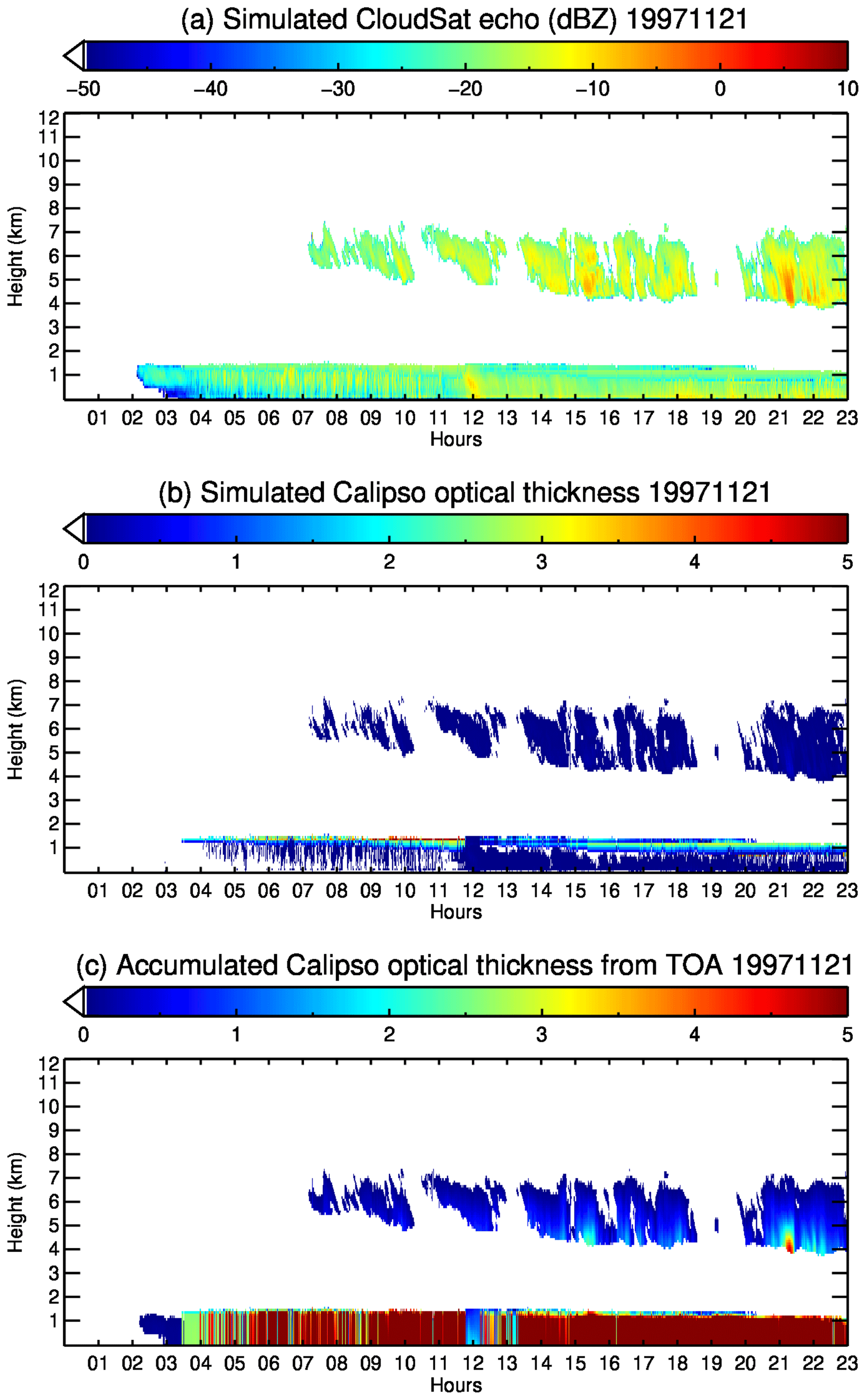
Figure 1 Simulated (a) CloudSat reflectivity and (b) CALIPSO cloud optical thickness, and (c) accumulated cloud optical thickness from the top of the atmosphere for CALIPSO on 21 November 1997 during the Surface Heat Budget of the Arctic Ocean (SHEBA) experiment.

The primary instrument aboard CALIPSO is a near-nadir view lidar, the CALIOP. CALIOP uses three receiver channels; one measures the 1064 nm backscatter intensity, and two channels measure the orthogonally polarized components of the 532 nm backscattered signal. The CALIOP can penetrate, and thus detect, clouds with optical thicknesses up to 5 (Winker et al., 2009). The cloud optical thickness was calculated based on retrieved cloud effective radius and cloud water content. For ice clouds, the cloud optical thickness, τ_i, was calculated by expressions of the following form:

$$\begin{array}{}\text{(1)}& {\mathit{\tau }}_{\mathrm{i}}=\underset{z_{\mathrm{1}}}{\overset{z_{\mathrm{2}}}{\int }}\mathrm{IWC}\mathrm{d}z\times \left(a_i+{\displaystyle \frac{b_i}{r_{\mathrm{e}}}}\right),\end{array}$$

where z₁ and z₂ are cloud base and cloud-top heights, IWC is the ice water content, r_e is the cloud effective radius, a_i and b_i are constants, and i is the spectral interval. For CALIOP wavelength, a_i and b_i are $\mathrm{3.448}\times {\mathrm{10}}^{-\mathrm{3}}$ m² g⁻¹ and 2.431 µmm² g⁻¹, respectively. Details of this approach can be found in Ebert and Curry (1992). For liquid clouds, the cloud optical thickness was calculated as follows:

$$\begin{array}{}\text{(2)}& \mathit{\tau }={\displaystyle \frac{\mathrm{3}{\int }_{z_{\mathrm{1}}}^{z_{\mathrm{2}}}\mathrm{LWC}}{\mathrm{2}{r}_{\mathrm{e}}{\mathit{\rho }}_{\mathrm{w}}}},\end{array}$$

where LWC is the liquid water content, and ρ_w is the water density (Dong et al., 1998). The vertical distribution of the estimated cloud optical thickness on 21 November 1997 is shown in Fig. 1b.

Figure 2 Typical (estimated) surface clutter profile adapted from Fig. 7 in Marchand et al. (2008) and thresholds used (blue line) in this study to detect clouds for CloudSat.

With the simulated vertical profiles of CloudSat reflectivity and cloud optical thickness, cloud masks for CloudSat, CALIPSO, and CloudSat and CALIPSO combined were derived with the following approach. The combined CloudSat and CALIPSO is referred to as CC hereinafter. A layer was flagged as being cloud if the simulated CloudSat reflectivity at a layer is larger than the mean radar-measured noise power at that layer, which is the 99th percentile of the clear-sky returns, as in Fig. 7 of Marchand et al. (2008) and Fig. 2 in this paper. The vertical line of the 99th percentile of the clear-sky returns serves as a threshold to detect clouds by CloudSat at all layers. This threshold provides a very stringent requirement for cloud detection, especially for cloud detection near the surface. Since it was suggested that the CloudSat cloud detection capability would be improved with lower mean radar-measured noise power near the surface (Marchand et al., 2008), in this study, the threshold was further lowered by 15 dBZe in the lowest five range bins (lower than 960 m), rather than the 99th percentile of the clear-sky returns, when higher than or equal to −26 dBZe (Marchand et al., 2008). For the CALIPSO cloud mask, any layer with a calculated cloud optical thickness larger than 0 and accumulated cloud optical thickness from TOA (Fig. 1c) less than 5 above this layer was flagged as cloud. It should be noted that a more sophisticated detection scheme is used in the operational CALIPSO cloud mask product (Winker et al., 2009) and operational CloudSat cloud mask (Marchand et al., 2008), and the results in this study should not be treated as the results from operational products. In the cloud mask with the CC, a layer was flagged as being cloud if the layer was flagged as being cloud by either sensor. The cloud mask on 21 November 1997 from CALIPSO, CloudSat, and CC are shown in Fig. 3. In this study, we calculated and examined the vertical profiles of cloud fraction from CALIPSO, CloudSat, and CC at layers from 150 m to 12 km. The mean cloud (ice cloud, liquid cloud, and mixed-phase cloud) fraction at a vertical layer was calculated as the ratio of the number of profiles identified as cloud (ice cloud, liquid cloud, and mixed-phase cloud) at this layer compared to the total number of profiles.

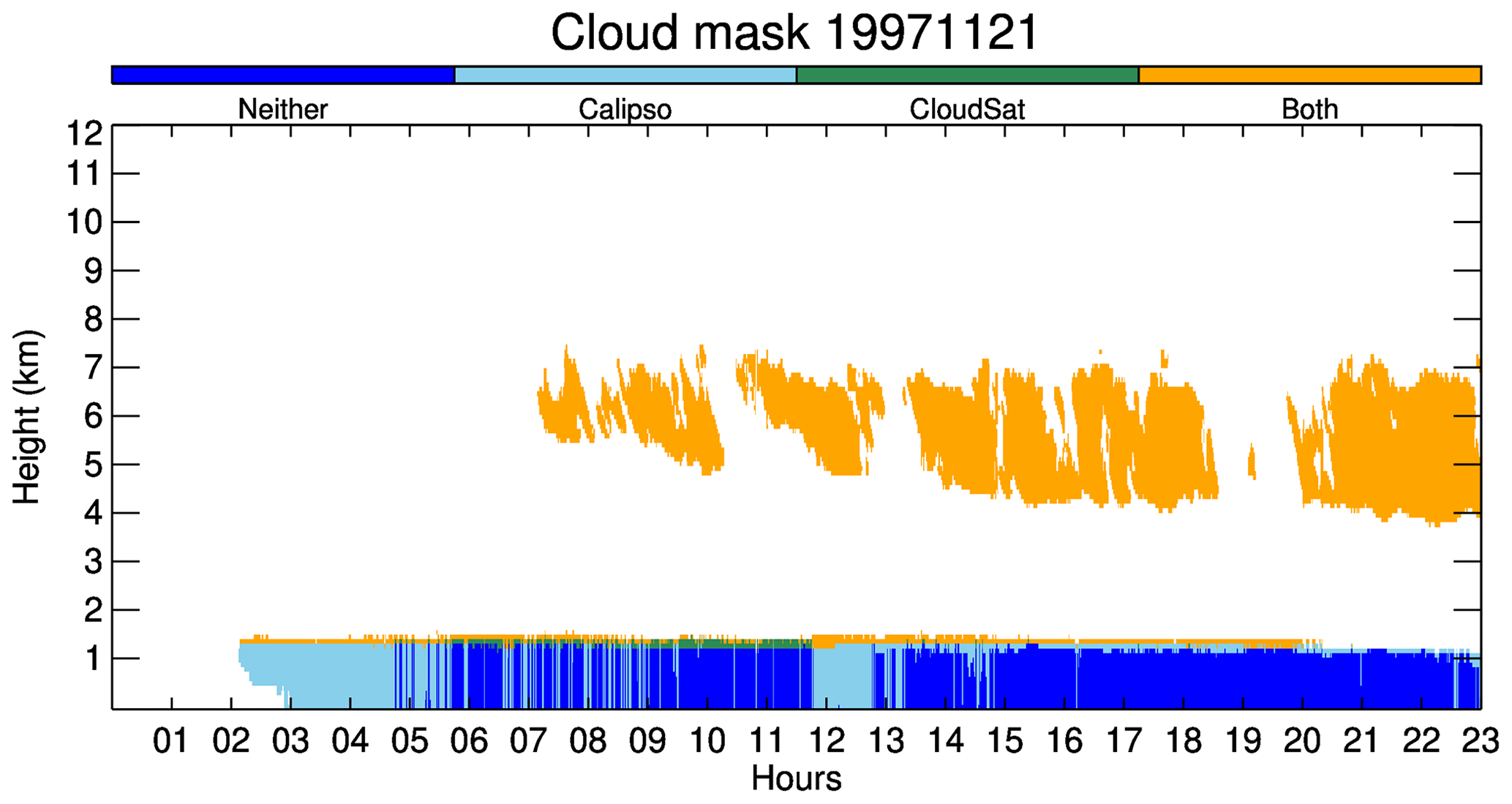
Figure 3 Cloud mask vertical profile based on simulated CloudSat reflectivity and cloud optical thickness for CALIPSO on 21 November 1997 collected during the SHEBA experiment.

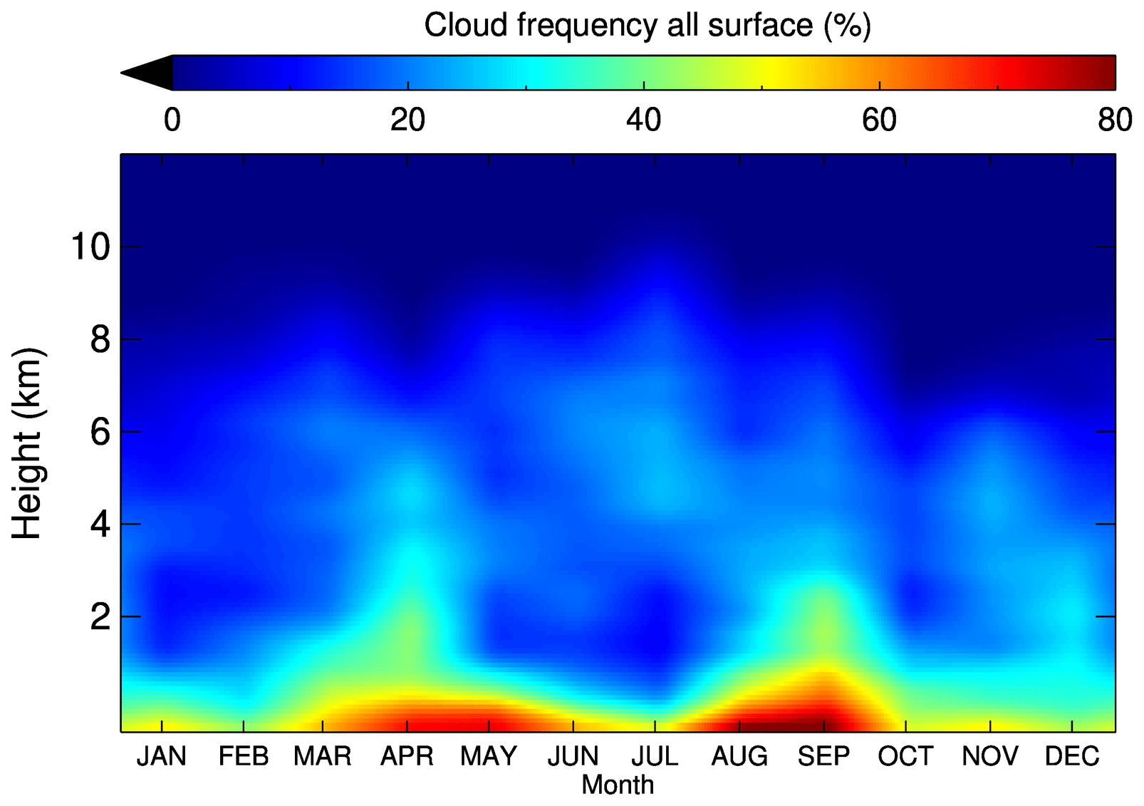
Figure 4 Mean cloud vertical distribution from the surface observations from October 1997 to October 1998 during the SHEBA experiment.

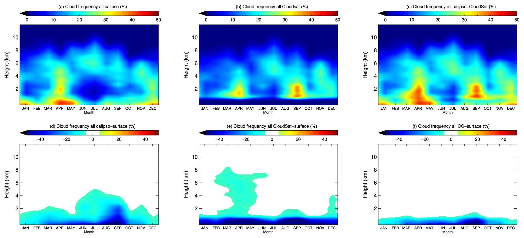
Figure 5 Cloud vertical distributions from (a) CALIPSO, (b) CloudSat, (c) combined CloudSat and CALIPSO, and the difference between (d) CALIPSO, (e) CloudSat, and (f) combined CloudSat and CALIPSO and surface observations during the SHEBA experiment.

There were two sets of cloud profiles used as inputs to a radiative transfer model. One set was the complete cloud profiles from the surface observations, including cloud classification, cloud effective radius, and cloud water content, which is referred to as surface cloud profile hereinafter. The other set was a subset of the cloud profiles including only those layers identified as clouds in the space-based radar, lidar, or combined lidar and radar cloud mask., which is referred to as the satellite cloud profile or CloudSat/CALIPSO/CC cloud profile, respectively. Outputs of the model include downward and upward longwave and shortwave radiation, shortwave and longwave cloud radiation fluxes, and cloud radiative forcing (CRF) at the surface and TOA. CRF is defined as the difference between the all-sky and clear-sky net radiation fluxes at the surface or TOA, which measures a cloud's impacts on the surface or TOA. Positive CRF at the surface (TOA) indicates that the clouds warm the surface (Earth–atmosphere system) relative to the clear skies, and negative CRF indicates that clouds cool the surface (Earth–atmosphere system). The radiative transfer model is Streamer (Key and Schweiger, 1998). Streamer can compute both radiance and irradiance under a wide variety of atmospheric and surface conditions (Liu et al., 2004; Loyer et al., 2021). A discrete ordinate solver is used to calculate the longwave and shortwave radiation fluxes. The surface type is selected as fresh snow, and the albedo is from a built-in spectral albedo model scaled by the surface broadband albedo from the surface observations. Albedo were computed for each hour during SHEBA by the Atmospheric Surface Flux Group (ASFG) radiometers (Intrieri et al., 2002a; Persson, 2002; Fig. S3). The monthly mean surface broadband albedos are lowest in July during the SHEBA experiment (Table S1 and Fig. S3 in the Supplement). The albedo for the cloud profile was set as the closest ASFG albedo. Streamer can simulate the radiation fluxes for up to 50 layers with cloud data. In this study, only layers from 150 m to 12.0 km are simulated. There are 125 layers from 150 m to 12.0 km in the retrieved cloud data sets, so that there are potential 125 layers with cloud data at maximum. Every layer with cloud data below 2.0 km was included in the Streamer input file, with cloud-top height, cloud physical thickness, cloud effective radius, and cloud water content; for cloud layers above 2.0 km, these cloud parameters were calculated for every five layers, including cloud-top height, cloud thickness, mean cloud effective radius, and water content for water and ice clouds, respectively. Hexagonal solid column was chosen as the shape of the ice clouds, and a sphere was chosen as the shape of liquid clouds. Though the ice cloud particle shape is different from that in QuickBeam, the ice cloud effective radius is the same as what used in the QuickBeam simulation. Temperature and moisture profiles come from the closest radiosonde, which were launched at least twice daily during the SHEBA experiment. The available cloud profiles have a temporal frequency of 1 min. In this study, the radiation fluxes are computed and shown using profiles with 15 min intervals (4 out of 60 profiles), and there are 96 cases in a day, except as otherwise stated. Daily means are computed based on the 96 values, and the monthly means are calculated based on the daily means.

The uncertainties in the radiation fluxes due to the omission of clouds from the space-based radar, lidar, or combined radar and lidar were estimated as being the difference between the radiation fluxes with partial and complete cloud profiles; all inputs of the radiative transfer model were the same for these two fluxes, except the inclusion/exclusion of the cloud layers that the space-based radar, lidar, or combined radar and lidar do not detect. The differences in these two fluxes can be used to quantify the impact of the space-based radar, lidar, or combined radar and lidar cloud detection limitations on the radiation fluxes at the surface and TOA. Rather than investigating all radiation fluxes, e.g., downward and upward longwave and shortwave radiation fluxes, this study focused on quantifying the uncertainties in the CRFs at the surface and TOA. In this paper, hereinafter, the differences in the CRFs means the differences between CRFs from satellite cloud profiles (CloudSat, CALIPSO, and CC) and the CRFs from surface cloud profiles. Positive differences indicate more warming effect, and negative differences indicate less warming effect or more cooling effect. The difference in the cloud amount, hereinafter, is the difference in the cloud amount from CloudSat, CALIPSO, and CC compared to the cloud amount from the surface observations. The space-based radar, lidar, or combined radar and lidar are interchangeable with CloudSat, CALIPSO, or CC (combined CloudSat and CALIPSO).

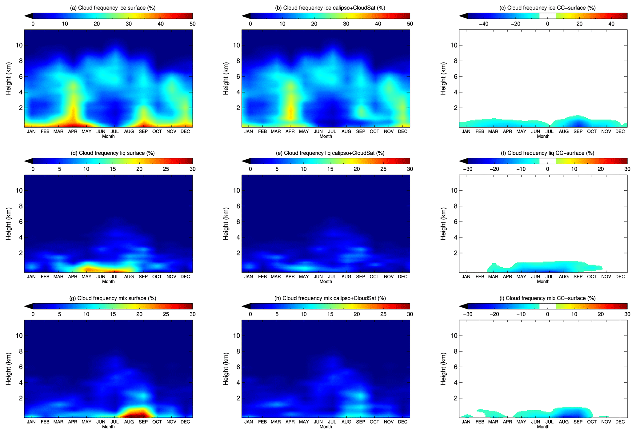
Figure 6 Cloud vertical distribution from surface observations for (a) ice, (d) liquid, and (g) mixed-phase clouds, from combined CloudSat and CALIPSO for (b) ice, (e) liquid, and (h) mixed-phase clouds, and their differences for (c) ice, (f) liquid, and (i) mixed-phase clouds during the SHEBA experiment.

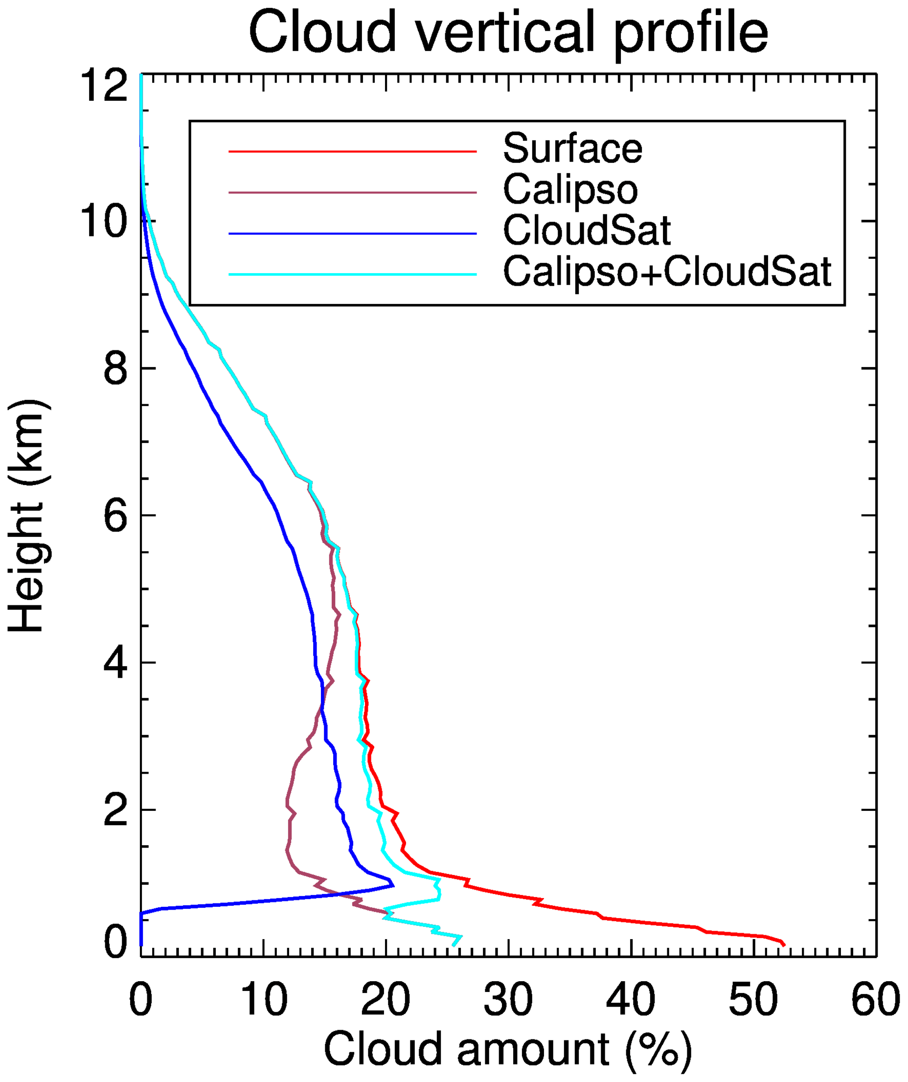
Figure 7 Mean cloud amount vertical distributions from surface observations, simulated CloudSat, CALIPSO, and CC during the SHEBA experiment.

3 Results

3.1 Cloud fraction vertical distributions

Mean cloud vertical distributions from SHEBA's surface observations show higher cloud amounts closer to the surface, mainly below 1 km (Fig. 4; same as Fig. 3b in Shupe et al., 2011). The high values near the surface show two maxima, i.e., one in August and September around at 80 % and another in April and May around 70 %. Mean cloud amounts above 2 km show high values in April, September, and in July towards higher altitudes. Local minima appear between 1.5 and 4 km in January, February, June–July, and October.

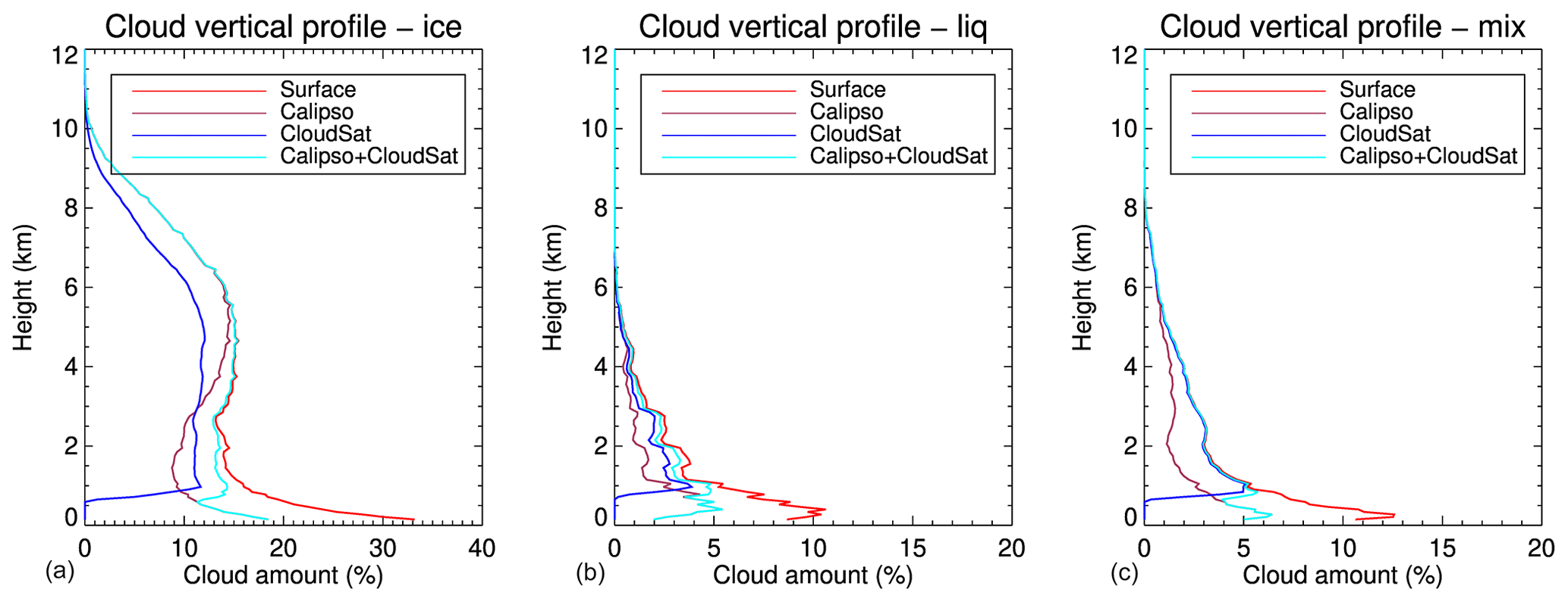
Figure 8 Mean cloud amount vertical distributions from surface observations and from simulated CloudSat, CALIPSO, and combined CloudSat and CALIPSO for (a) ice, (b) liquid, and (c) mixed-phase clouds during the SHEBA experiment.

Figure 5 shows the cloud vertical distribution from CALIPSO, CloudSat, and CC and their differences with surface observations. Above 1 km, CloudSat detects most of the clouds identified via surface observations (Fig. 5b), with most of the differences between 0.0 % to −5.0 % (Fig. 5e). The exceptions are in April, when CloudSat shows much lower cloud amounts between 1 and 8 km, with the differences between −5.0 % to −8.0 %. These negative differences are collocated with the higher amounts of ice clouds (Fig. 6a), consistent with the fact that CloudSat has limited sensitivity to optically thin ice clouds (Stephens et al., 2002). CALIPSO also detects most of the clouds seen from surface sensors (Fig. 5a), with most of the differences between 0.0 % and −5.0 %, except that CALIPSO detects much fewer clouds between 1 and 4.5 km from June to September, with maximum negative differences in September. These large negative differences are collocated with the higher amount of liquid and mixed-phase clouds between 1 and 6 km from June to September (Fig. 6d, g), which have high cloud optical thickness and saturate the CALIPSO signal for the clouds below. The CC detects all the clouds that surface observations show (Fig. 5c, f), with differences between 0.0 % and −1.0 %, except for fewer clouds between 1 and 2 km in August and September with differences between −8.0 % and −3.0 %.

Below 1 km, the CloudSat detects much fewer clouds than the surface observations because of surface clutter (Fig. 5e). The percentage of clouds that CloudSat detects compared to the surface observations is 0 % below 600 m for all months and gradually increases to around 75 % near 1 km for most months, with similar results for ice, liquid, and mixed-phase clouds for all months. CALIPSO detects some clouds under 1 km, depending on the accumulated cloud optical thickness above. In winter, the most common cloud types are ice clouds, which have relatively small cloud optical thicknesses; thus, CALIPSO can detect some clouds near the surface, e.g., around 80 % in December and January and around 60 % in other winter months. While in summer the liquid and mixed-phase clouds at higher levels often have high optical thicknesses and saturate the CALIPSO signal above 1 km, CALIPSO detects limited clouds near the surface, e.g., around 30 % in September and 40 % in other summer months. The CC approach takes advantage of the detection capability of both CloudSat and CALIPSO. However, because of the poor detection capability of CloudSat near the surface, especially below 600 m, the CC detects similar amounts of clouds as that of CALIPSO alone, especially below 600 m.

The annual mean cloud amount vertical profiles (Fig. 7; Table S2) show similar features for cloud detection capabilities from CloudSat, CALIPSO, and CC as those illuminated in the time–height cloud amount distributions (Figs. 5, 6). Below 600 m, the CloudSat cloud amount is 0.0 %, so the CC cloud detection capability comes from CALIPSO, which detects roughly half of the clouds detected by the surface observations and 25 % less in mean absolute values (Table S2). From 600 m to 1 km, CloudSat's detection capability increases, while CALIPSO sees slightly above 50 % of all the clouds detected by surface observations, and the differences between the CC cloud amount and those from surface observations drop from −16.2 % to −2.7 %, which is roughly 9 % less in mean absolute values. From 1 to 2 km, the CALIPSO and CloudSat detection capabilities continue to improve, and their combination detects almost all the clouds seen in surface observations with differences between −2.7 % and −1.3 %. Above 2 km, the CloudSat has slightly lower cloud amounts than that from the surface due to thin ice clouds that remain undetected, while CALIPSO's detection capability increases because of the smaller accumulated cloud optical thickness above. As a result, the CC detects most of the clouds that surface observation sees above 2 km and the majority of the clouds above 1 km.

Ice clouds have a similar time–height distribution to that of all clouds (Fig. 6a). High cloud amounts in April and December appear above 1 km; while not all of them can be detected by CloudSat, these clouds can be detected by CALIPSO due to the low cloud optical thickness above. The CC detects most of the clouds that surface observations see, except below 1 km (Fig. 6b, c). Liquid clouds are most common in the lowest 1 km, mainly from April to September; they also appear in higher altitudes from June to September, e.g., around 9 % at 2750 m in September (Fig. 6d). The CC detects most liquid clouds above 1 km, with the differences from the surface observations less than 1.0 % in most months. The major negative differences are below 1 km from March to October (Fig. 6e, f). The mixed-phase clouds are most common in the lowest 1 km, mainly in August and September, but also appear in higher altitudes from June to September (Fig. 6g). The CC detects most mixed-phase clouds above 1 km, with the differences from surface observations being less than 0.5 % in all months. The major negative differences are below 600 km from May to October (Fig. 6h, i). These features are reflected in the mean cloud amount vertical profiles for ice clouds, liquid clouds, and mixed-phase clouds, respectively (Fig. 8 and Table S3).

The mean cloud vertical profiles for all, ice, liquid, and mixed-phase clouds in the winter months (November to March; Fig. S4a–d) and the summer months (May to September; Fig. S4e–h) show similar features as those for all months (Figs. 7, 8). Mean overall cloud amounts in the summer months have higher values at all levels, especially below 1 km, mainly due to higher liquid clouds and mixed-phase clouds. The CloudSat mean cloud amounts above 1 km are smaller than those from the surface observations, with relatively constant differences between 3.0 %–4.0 % due to not detecting thin ice clouds. The differences between CALIPSO and the surface cloud amount increase with decreasing altitude due to the increasing accumulated cloud optical thickness. The CC detects most of the clouds that surface observations see above 1 km but much fewer below 1 km, mainly due to the surface clutter effect of CloudSat and limited CALIPSO detection capability below 1 km. Because of more liquid clouds, mixed-phase clouds, and even ice clouds in higher altitudes and the associated higher accumulated cloud optical thickness above 1 km in the summer months than in the winter months, the differences in cloud amount between the CC and the surface observations are larger in summer months than in winter months.

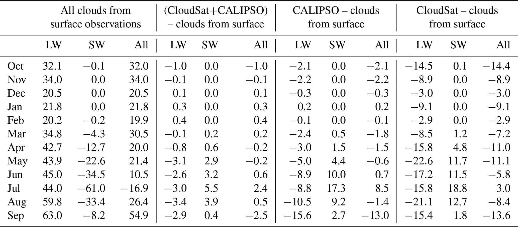
Table 1 Monthly mean CRF at the surface for longwave (LW), shortwave (SW), and the combined LW and SW (all) with the clouds from the surface observations collected during the SHEBA experiment and the differences between the CRF with clouds in the surface observations only identified from combined CloudSat and CALIPSO, CALIPSO, or CloudSat and the CRF from the clouds from the surface observations.

3.2 Uncertainty in CRF due to cloud detection limitations near the surface

3.2.1 Surface

During the SHEBA experiment, CRFs, computed with complete cloud profiles, are positive most of the year, except around 40 d centered on Julian day 560, starting from 1 January 1997 (Fig. 9). This is mostly due to the lack of sunlight during winter months leading to the longwave heating being the dominant term. As a result, the monthly mean CRFs are positive in all months except in July (Fig. S5; Table 1). This result suggests that clouds warm the surface for most of the year, except for a short time in July over the Arctic Ocean, which is consistent with the conclusions of previous studies (Intrieri et al., 2002a; Shupe and Intrieri, 2004). There are two major components of the CRF, namely longwave (LW) and shortwave (SW) CRFs. The longwave CRFs are positive all year, with the maximum in September and the minimum in February. The shortwave CRFs are zero from October to February due to little incoming shortwave radiation and are negative in other months. The maximum negative values of the shortwave CRF are in July 1998 (Fig. S5; Table 1), which can be attributed to the combination of the near-maximum accumulated TOA incoming shortwave radiation flux and the minimum surface albedo in July during the SHEBA experiment (Letterly et al., 2018; Shupe and Intrieri, 2004).

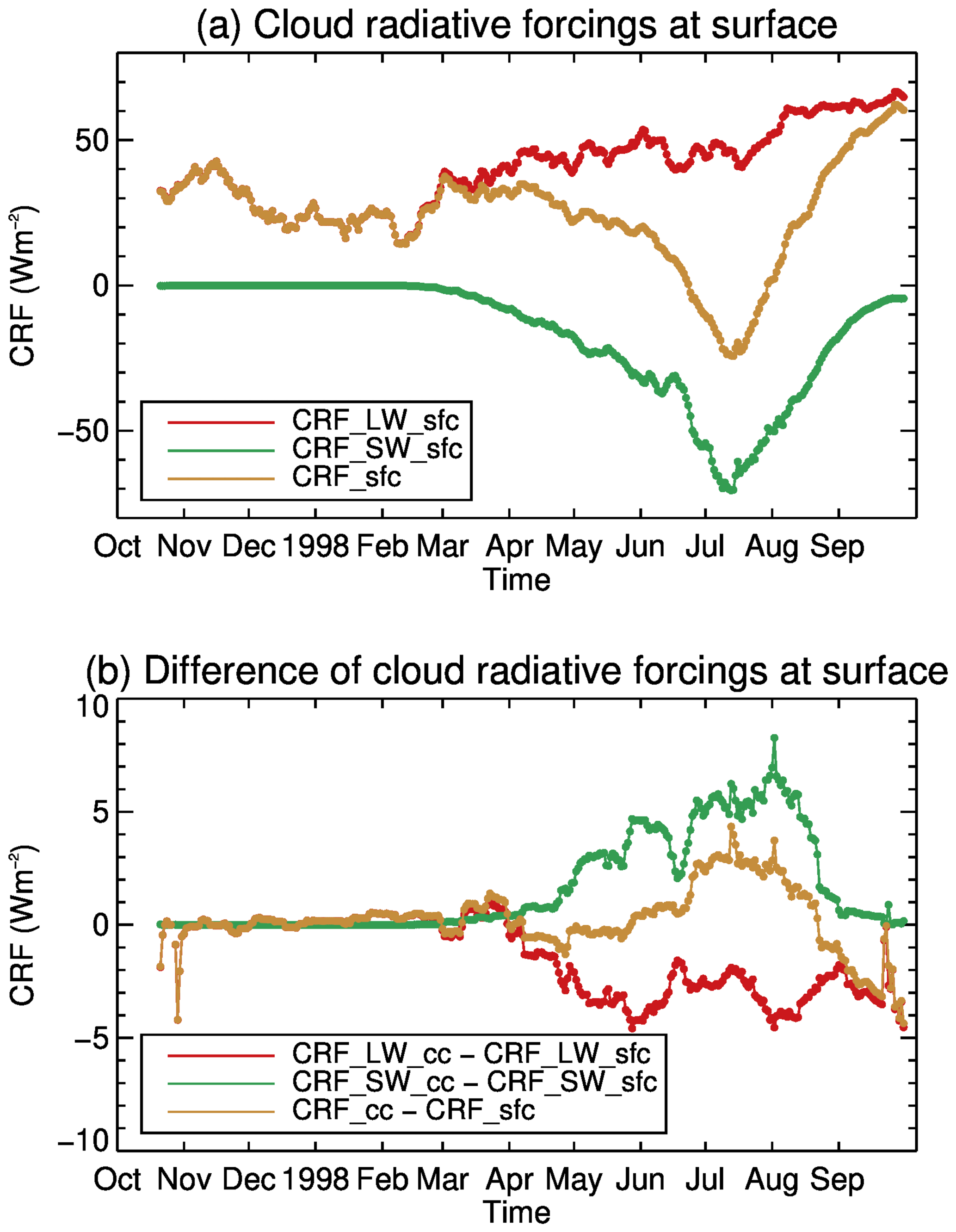
Figure 9 (a) CRF with a 20 d running average of daily means at the surface for longwave (LW) and shortwave (SW) with clouds from surface observations collected during the SHEBA experiment and (b) CRF differences with clouds identified by the combined CloudSat and CALIPSO (CC) and all clouds from surface observations.

Figure 10 Histogram of longwave cloud radiative forcing at the surface using clouds identified by combined CloudSat and CALIPSO and using clouds from surface observations during the SHEBA experiment for (a) January to December, (b) November to March, and (c) May to September. Ratios of cases with absolute differences less than 1 Wm⁻² to all cases are 69.1 %, 81.5 %, and 59.7 %, for panels (a), (b) and (c), while being excluded from the histogram.

CRFs computed with cloud profiles identified by the CC cloud mask show a very similar annual cycle and values to those using complete cloud profiles (Fig. 9; Table 1). Their absolute differences are less than 3 Wm⁻² for all months, with a maximum of 2.5 Wm⁻² in September and 2.4 Wm⁻² in July. The differences in their longwave CRFs are mostly near zero in the winter months, with larger negative values from May to September (Fig. S5; Table 1). The differences in their shortwave CRF are positive and larger in the summer months but zero in the winter months. The cancellation of the shortwave and longwave CRF differences in the summer months and both differences being near zero in the winter months lead to smaller CRF differences.

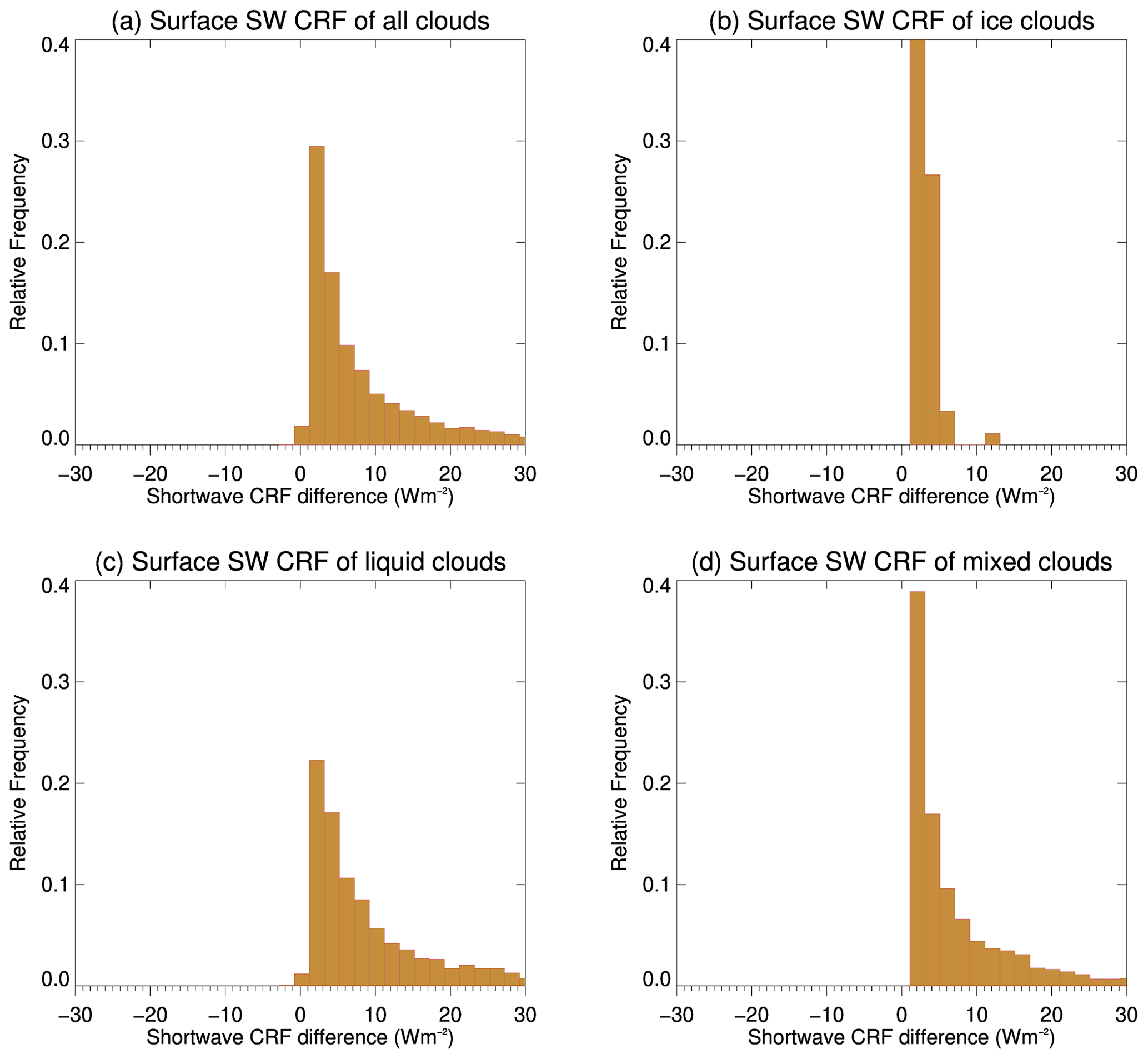
Figure 11 Histogram of shortwave cloud radiative forcing at the surface using clouds identified by combined CloudSat and CALIPSO and clouds from surface observations during the SHEBA experiment for (a) all clouds, (b) ice clouds, (c) liquid clouds and (d) mixed-phase clouds. Ratios of cases with absolute differences less than 1 Wm⁻² to all cases are 40.5 %, 91.3 %, 18.4 %, and 39.6 %, for panels (a), (b), (c) and (d), while being excluded from the histogram.

Though the differences in monthly mean CRFs are small, large ranges in both the longwave and the shortwave CRFs exist in individual values, calculated using the individual 1 min interpolated profiles (Fig. 10). The longwave CRFs at the surface in the winter months, November to March, mostly (81.5 %) have absolute differences within 1 Wm⁻², with limited cases outside that range (Fig. 10b); the same conclusion holds for clouds being ice, liquid or mixed-phase clouds. Please note that cases with absolute differences less than 1 Wm⁻² are the majority, while being excluded from the histogram in Fig. 10. In the summer months, the differences in the longwave CRFs at the surface show mostly negative values as large as −30 Wm⁻² (Fig. 10). These differences are more negative if liquid or mixed-phase clouds are not detected near the surface. The differences in the shortwave CRFs are all positive, as large as 30 Wm⁻², in the summer months (Fig. 11a), and are small (large) if ice (liquid or mixed-phase) clouds are not detected near the surface (Fig. 11b, c, d).

When the cloud profiles determined from only the CloudSat cloud mask are used, the differences in the CRFs are much larger than the differences when using the cloud profiles determined from the CC (Table 1), e.g., −14.4 Wm⁻² in October and −13.6 Wm⁻² in September. The differences in the longwave and shortwave CRFs are even larger, which cancel each other out somewhat for smaller CRFs. When the cloud profiles determined from only the CALIPSO cloud mask are available, the differences in the CRFs are smaller than the differences with cloud profiles from only the CloudSat and larger than the differences with the CC. For example, the differences are 8.5 Wm⁻² in July and −13.0 Wm⁻² in September. The differences in the longwave CRFs have large negative values, and the differences in shortwave CRFs have large positive values, which cancel each other out for smaller CRFs (Table 1).

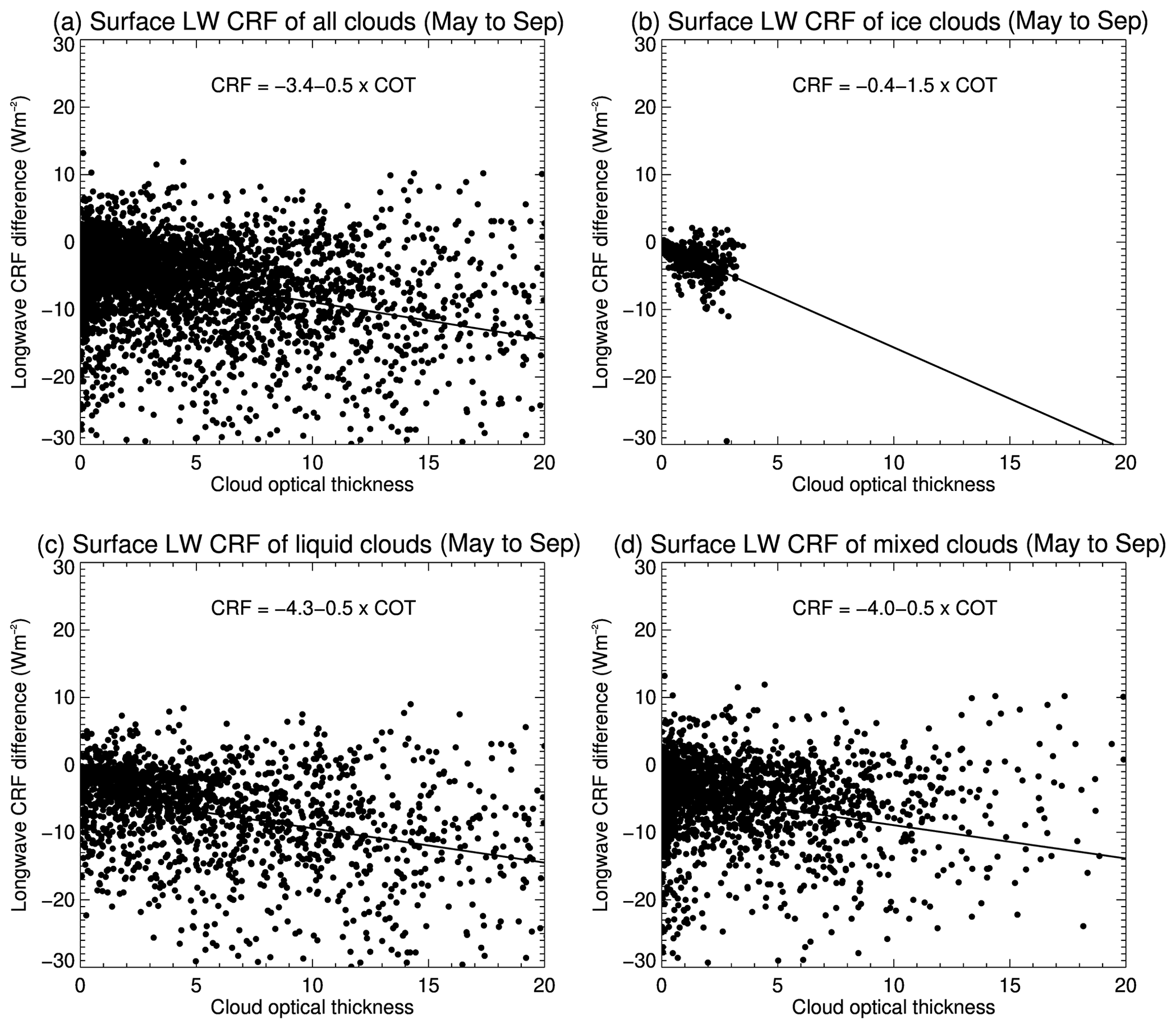
Figure 12 Scatterplots of longwave cloud radiative forcing at the surface using clouds identified by combined CloudSat and CALIPSO and clouds from surface observations and cloud optical thickness for (a) all clouds, (b) ice clouds, (c) liquid clouds, and (d) mixed-phase clouds below 1 km from May to September during the SHEBA experiment.

The longwave CRF differences at the surface are close to zero in the winter months and tend more towards large negative values in the summer months, especially with liquid and mixed-phase clouds near the surface (Fig. 10). In the summer months, the longwave CRF differences become largely negative with the increasing cloud optical thickness below 1 km and those clouds not being detected by the CC (Fig. 12). In the winter months, temperature inversions are relatively weaker under cloudy conditions (Fig. 13a), and the cloud effective temperature is close to the surface temperature in a well-mixed boundary layer (Tjernström and Graversen, 2009). Removal of some of these lower-level clouds would not likely greatly change the downward longwave radiation at the surface as long as there are clouds with a similar effective temperature on top of these undetected clouds, which leads to the small longwave CRF differences in the winter months. While in the summer months the temperature inversions are not as common, the clouds in the lowest 1 km often have temperatures lower than the surface, with even lower cloud temperatures above 1 km (Fig. 13b). Removal of more clouds near the surface would lead to less downward longwave radiation and thus smaller longwave CRFs and larger negative differences.

The SW CRF differences at the surface are positive in the summer months, especially when omitting liquid and mixed-phase clouds near the surface (Fig. 11). Larger positive SW CRF differences are associated with increasing optical thickness of those clouds below 1 km and not detected by the CC (Fig. 14). In the summer months, especially in June, July, and August, the surface albedo decreases due to the melt ponds and more open water; the surface absorbs more shortwave radiation without clouds above. Clouds, especially those that are liquid and mixed phase, are brighter than the surface and reflect more shortwave radiation back to space, thus leading to smaller downward shortwave radiation at the surface and larger negative shortwave CRFs. Removal of more clouds near the surface would lead to larger downward shortwave radiation, smaller negative shortwave CRFs, and larger positive differences.

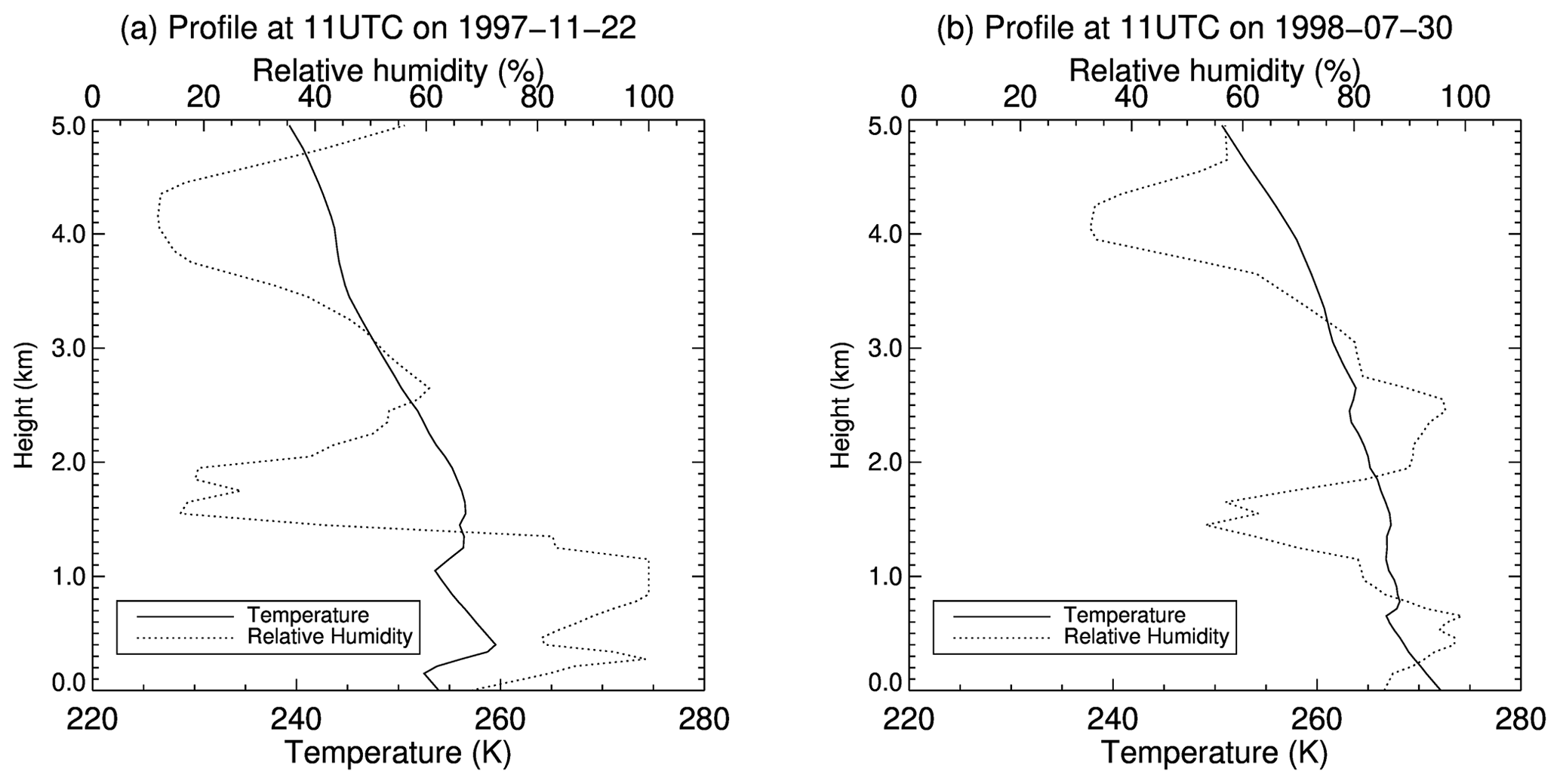
Figure 13 Temperature and relative humidity profiles on (a) 21 November 1997 and on (b) 30 July 1998 over the Arctic Ocean during the SHEBA experiment.

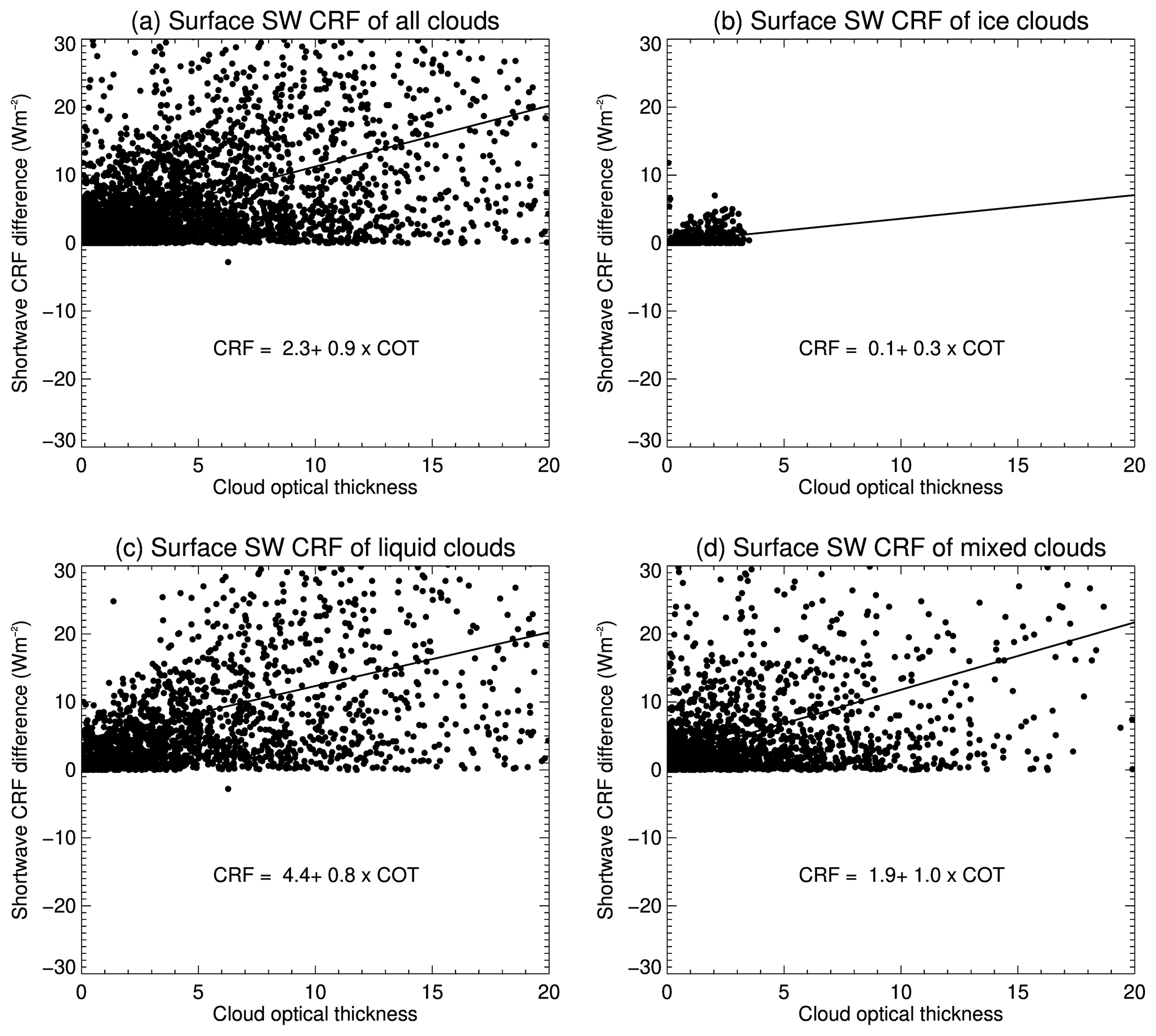
Figure 14 Scatterplots of shortwave cloud radiative forcing at the surface using clouds from surface observations and clouds identified by combined CloudSat and CALIPSO and cloud optical thickness of omitted (a) all clouds, (b) ice clouds, (c) liquid clouds, and (d) mixed-phase clouds below 1 km during the SHEBA experiment.

Table 2 Monthly mean CRF at the TOA for longwave (LW), shortwave (SW), and the combined LW and SW (all) with the clouds from the surface observations collected during the SHEBA experiment and the differences between the CRF with clouds in the surface observations only identified from combined CloudSat and CALIPSO, CALIPSO, or CloudSat and the CRF from the clouds from the surface observations.

3.2.2 Top of the atmosphere (TOA)

CRFs at TOA are negative from April to August and positive from September to March during the SHEBA experiment (Figs. 15, S6; Table 2). The absolute of the negative values is much larger than the absolute of the positive values. This suggests the clouds cool the Arctic Ocean in the summer months, except September, and slightly warm the Earth in the winter months, with an overall impact of cooling the Arctic Ocean. The clouds in the summer months reflect more shortwave radiation back to space than surface, especially in July when the surface albedo is low due to melt ponds and more open water, such that the shortwave CRFs at TOA are all negative in the summer months. On the other hand, the longwave CRFs at TOA are positive in all months. This is possibly due to colder effective cloud-top temperature than the effective emitting temperature from the combined atmosphere and surface, even in the winter months when surface temperature inversions are common. The shortwave and longwave CRFs somewhat cancel each other out in most months.

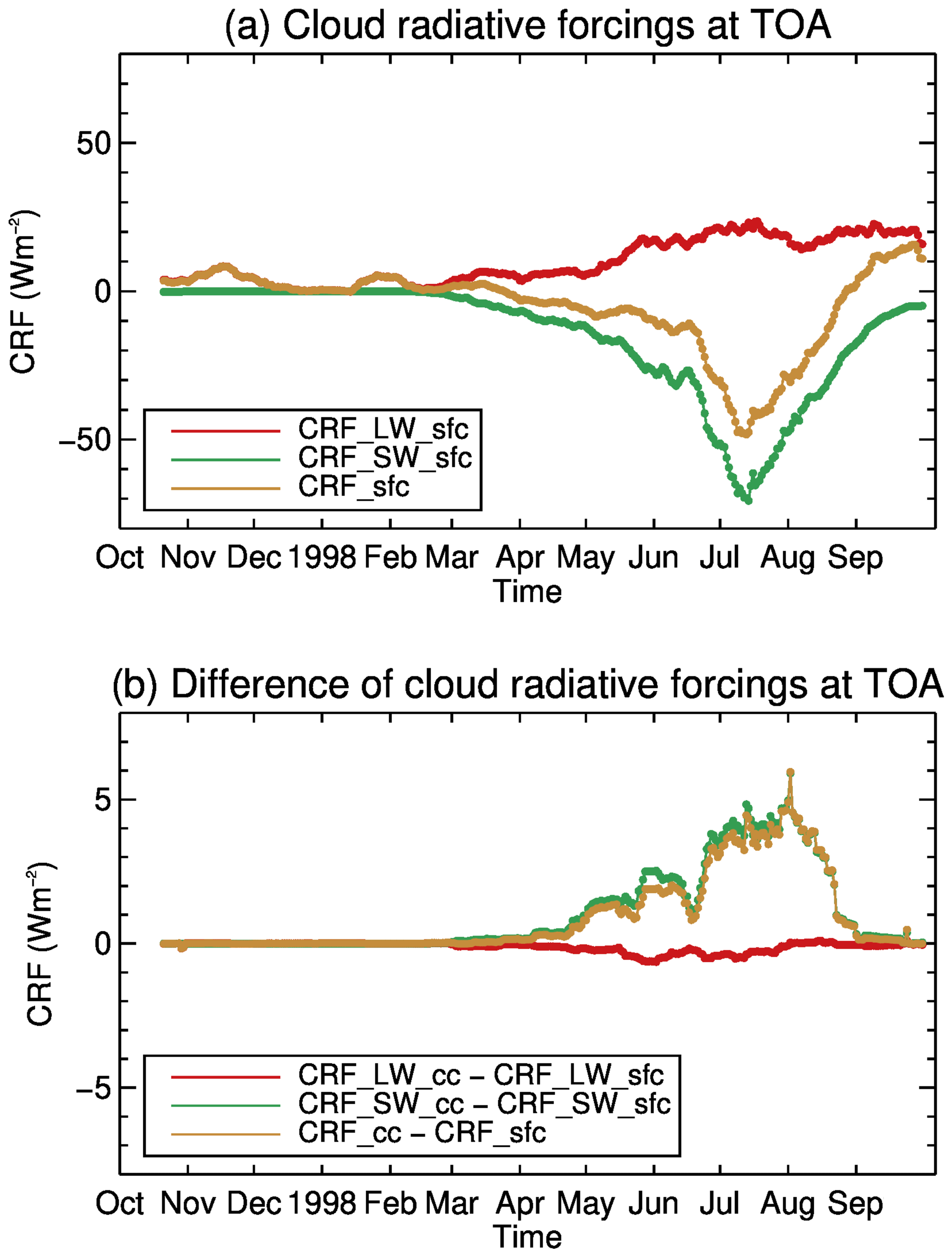
Figure 15 (a) CRF with a 20 d running average of daily means at the TOA for LW and SW, with clouds from surface observations collected during the SHEBA experiment, and (b) CRF differences with clouds identified by the combined CloudSat and CALIPSO (CC) and all clouds from surface observations.

For the impact of the cloud detection limitation near the surface by the CC, the CRF differences are positive in all months, with the maximum monthly mean difference at 3.4 Wm⁻² in July. The differences in the longwave CRFs are near zero in all months, with the maximum magnitude in July at −0.7 Wm⁻², which indicates that the contribution of clouds not detected near the surface is insignificant to the LW radiation at TOA. The differences in the shortwave CRFs are all positive, with larger values than the longwave CRF differences, with the maximum magnitude in July at 4.1 Wm⁻². The CRFs are determined by the shortwave CRFs because of the much smaller longwave CRFs. The differences in shortwave CRFs are all positive and in the summer months (Fig. 16a), and these differences are larger if liquid, or mixed-phase, clouds are not detected near the surface (Fig. 16b, c). A few cases exist where only ice clouds are not detected near the surface.

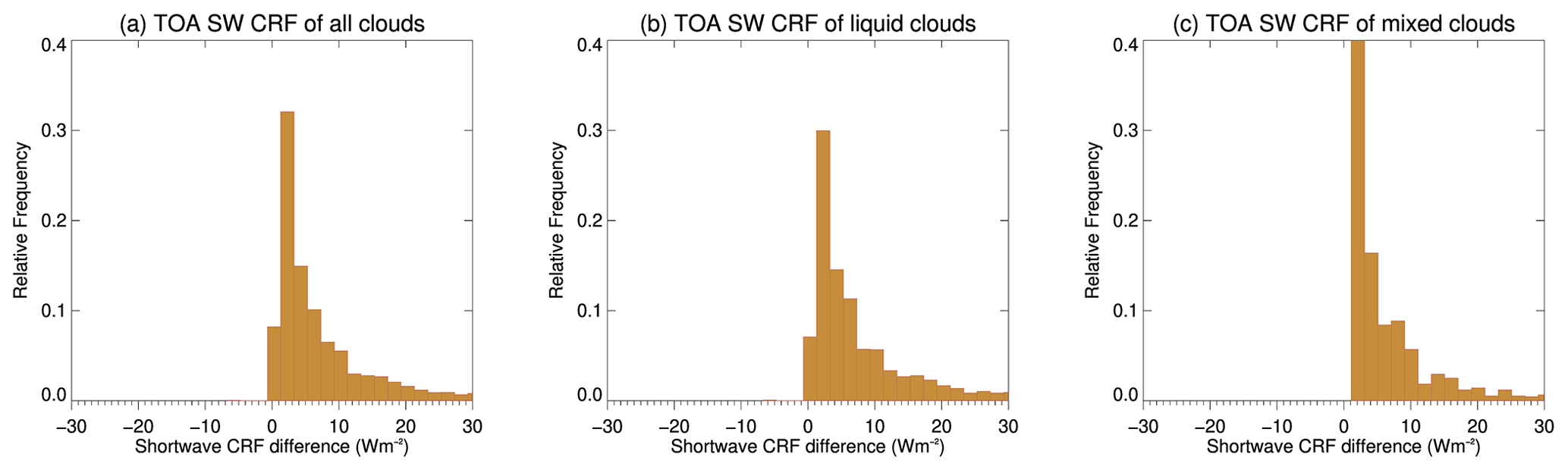
Figure 16 Histogram of shortwave cloud radiative forcing at the TOA between using clouds from surface observations and clouds identified by combined CloudSat and CALIPSO for (a) all clouds, (b) liquid clouds, and (c) mixed-phase clouds during the SHEBA experiment.

When cloud profiles from only the CloudSat cloud mask are available, the differences in the CRFs from CloudSat become much larger than the differences using the CC (Table 2), e.g., 13.9 Wm⁻² in July for only CloudSat compared to 3.4 Wm⁻² in July for the CC. When cloud profiles from only the CALIPSO cloud mask are available, the differences in CRFs from CALIPSO are smaller than those from only CloudSat and larger than those from the CC, e.g., 13.4 Wm⁻² for CALIPSO in July. For both, the differences in the longwave CRFs are not affected much, while the differences in the shortwave CRFs become large positive values. These changes in the shortwave CRFs determine the CRFs changes (Table 2).

The cloud detection limitations near the surface by the CC do not affect the longwave CRFs at TOA but lead to positive shortwave CRF differences at TOA (Fig. 16). These positive differences are larger with the increasing optical thickness of those clouds below 1 km and are not detected by the CC (Fig. 17). In the summer months, the surface albedo decreases, which means the surface reflects less shortwave radiation in clear-sky conditions. Clouds, especially those that are liquid and mixed phase near the surface, help brighten the clouds so that they reflect more shortwave radiation back to space, which leads to larger upward shortwave radiation at the TOA and negative shortwave CRFs. Removal of clouds near the surface would reduce the brightness of the cloud, resulting in smaller upward shortwave radiation at TOA, smaller negative shortwave CRFs, and thus positive differences.

3.3 Uncertainty in the results

The CloudSat and CALIPSO cloud masks are based on the simulated radar reflectivity and cloud optical thickness using the retrieved cloud properties from the surface-based combined radar and lidar observations during the SHEBA experiment. For CloudSat, a vertical profile of fixed thresholds is applied to identify the CloudSat cloud mask, and a layer with radar reflectivity higher than the threshold at that layer is identified as being cloud; for CALIPSO, a layer with cloud optical thickness larger than 0 and an accumulated cloud optical thickness from TOA to the layer above this layer which is less than a fixed threshold, i.e., 5, is identified as cloud. There are also uncertainties in the cloud property retrievals. In addition, the surface-based radar and lidar observations are usually reasonable only at heights greater than 100–150 m above ground (Griesche et al., 2021; Hu et al., 2021). However, these profiles of cloud properties serve as a reasonable data set of possible Arctic cloud scenarios covering a whole year, which also serve as a reasonable data set to conduct this study. Retrieval uncertainties in these cloud properties do not affect the main conclusion of this study.

Radiative flux computations shown above are based on profiles with 15 min intervals. Calculations were also made using profiles with 1 h intervals (1 out of 60 profiles) to produce the daily means and monthly means. All the conclusions are the same, with the maximum differences in the CRFs at the surface less than 0.6 Wm⁻² and even less for those at the TOA from the monthly means from the profiles with 15 min intervals and 1 h intervals (Table S4). This demonstrates that computations using profiles with 15 min intervals may be sufficient to describe the cloud detection limitations on the radiative flux estimations.

There are a few factors leading to uncertainties in the CloudSat and CALIPSO cloud masks and, consequently, the derived cloud amounts and computed radiation fluxes based on these masks. These factors include the accuracy of the simulated radar reflectivity and the cloud optical thickness, and the cloud detection methods for CloudSat and CALIPSO. It is challenging to evaluate these uncertainties because of the lack of truth data, e.g., scarcity of the collocated cloud observations from in situ cloud measurements and surface-based and space-based radar–lidar cloud observations. Many studies have shown the capability of QuickBeam to simulate CloudSat reflectivity (Bodas-Salcedo et al., 2011; Zhang et al., 2018). Even though there were no CloudSat data in 1997 and 1998 to validate the simulated CloudSat reflectivity, there were surface-based MMCR observations at 35 GHz. Instead of validating simulated CloudSat reflectivity, we compared the surface-based MMCR observations to the simulated radar reflectivity at 35 GHz at the surface. Their differences reflect the combined uncertainties in the cloud property retrievals and the QuickBeam simulations. Such a case is shown in Fig. S7. Results show small differences for ice cloud reflectivity and relatively large differences for liquid cloud reflectivity. Further tests show the large differences when liquid cloud became smaller when the smaller liquid cloud effective radius was used in the simulation. This might indicate there are higher uncertainties in the liquid cloud effective radius retrievals for this specific case.

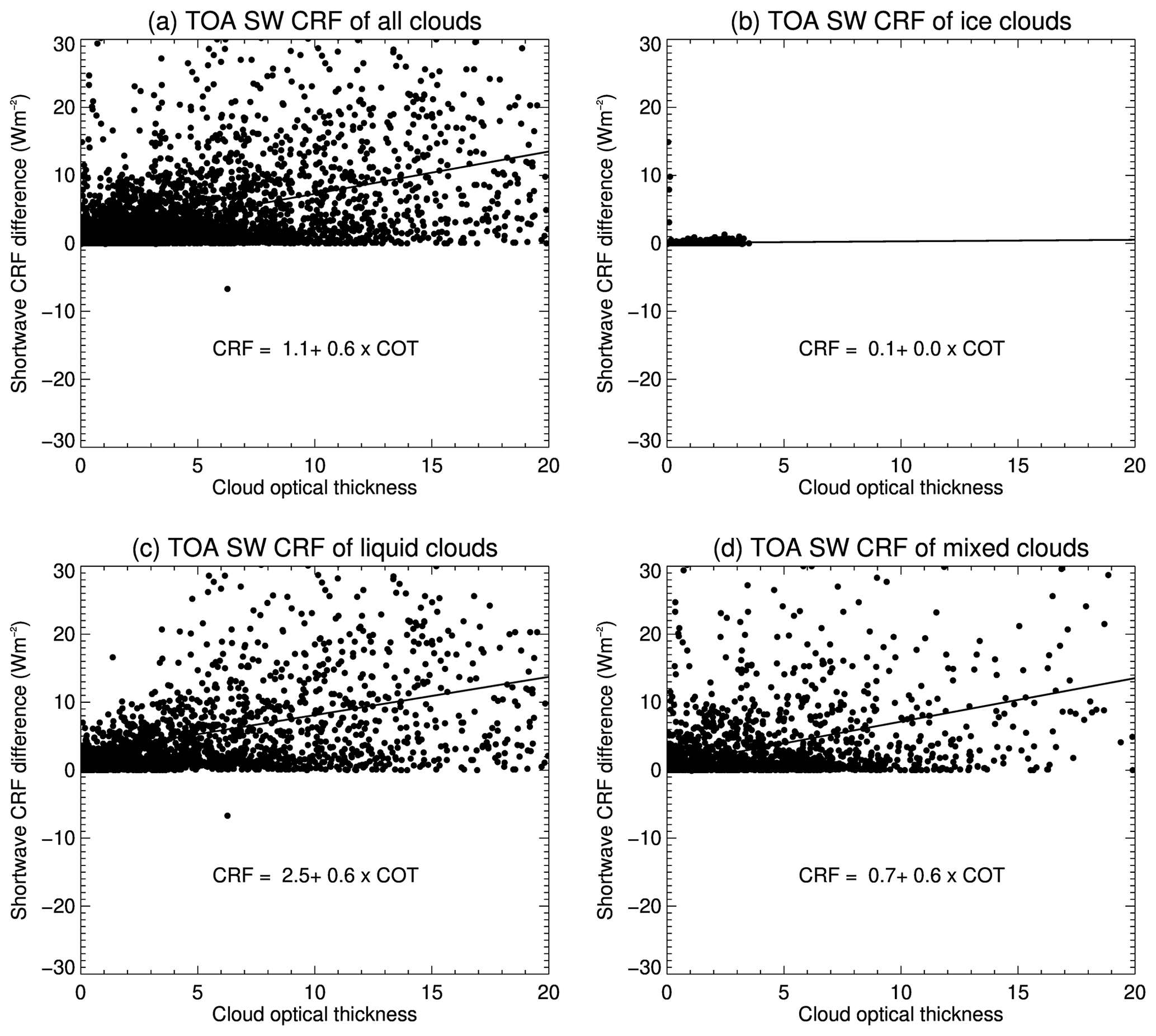
Figure 17 Scatterplots of shortwave cloud radiative forcing at the TOA between using clouds from surface observations and clouds identified by combined CloudSat and CALIPSO and cloud optical thickness of omitted (a) all clouds, (b) ice clouds, (c) liquid clouds, and (d) mixed-phase clouds below 1 km during the SHEBA experiment.

The CALIPSO cloud detection capability depends on the threshold of the accumulated cloud optical thickness, and different thresholds have been applied in previous research (Hu et al., 2007). A cloud optical thickness threshold of 5 is used in this study. Different thresholds, e.g., 4 and 6, are applied to estimate the CALIPSO cloud detection sensitivity to this threshold. The mean cloud amount vertical profiles with thresholds of 4, 5, and 6 are presented in Fig. 18 for all clouds, ice clouds, liquid clouds, and mixed-phase clouds. With a smaller (larger) threshold, the CALIPSO cloud amounts are smaller (larger) because the CALIPSO detects fewer (more) clouds at the lower levels. The cloud amount differences are −3.0 % (3.0 %) at 149.5 m, −1.7 % (1.7 %) at 1050 m, and around 0 % at 6050 m for all clouds, −2.0 % (2.0 %) at 149.5 m, 1.0 % (−1.0 %) at 1050 m, and around 0 % at 6050 m for ice clouds, and −0.5 % (0.5 %) at 149.5 and 1050 m, and around 0 % at 4050 m for liquid and mixed-phase clouds. The impacts of the CALIPSO threshold changes on the monthly CRFs at the surface and the TOA are also investigated. Results show that, with increasing CALIPSO cloud detection capability, e.g., increasing thresholds, the LW (SW; total) monthly CRF differences become smaller negative (positive; overall; Table S5). Lidar with stronger cloud detection capability is desirable for better radiative flux estimations at the surface and the TOA.

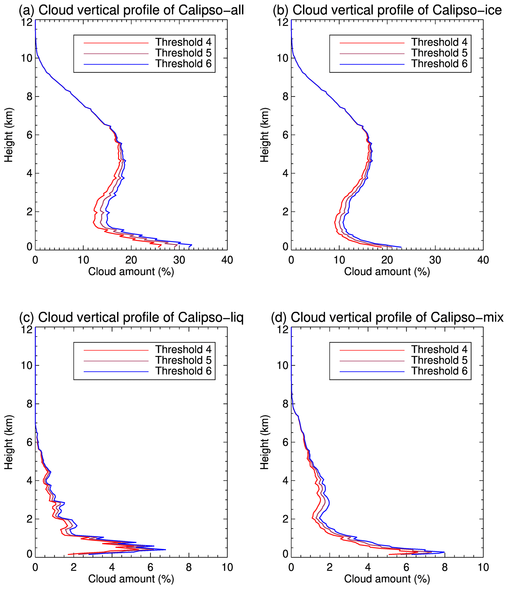
Figure 18 CALIPSO cloud amount vertical profile with three optical thickness thresholds of 4, 5, and 6 for (a) all, (b) ice, (c) liquid, and (d) mixed-phase clouds.

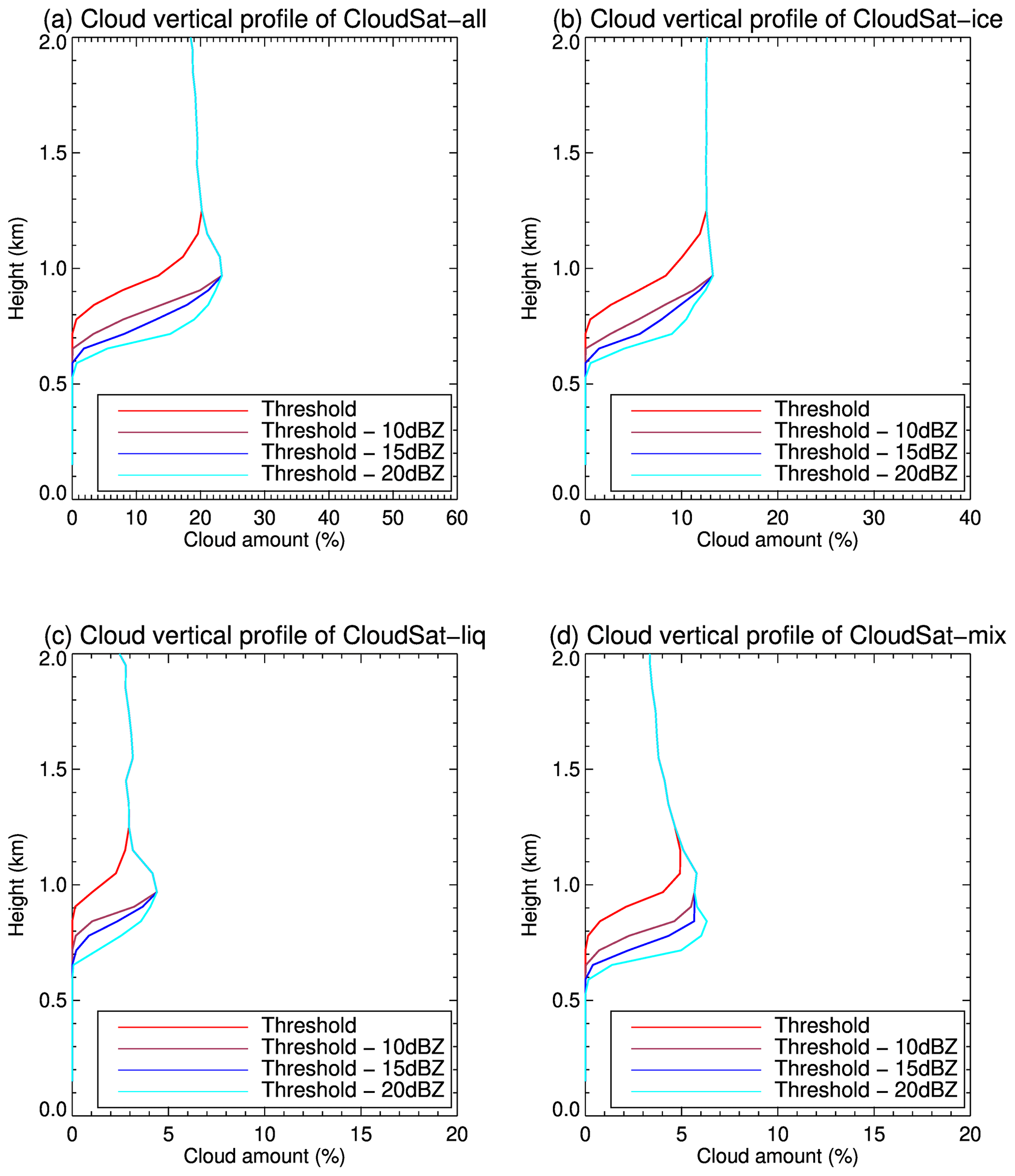
Figure 19 CloudSat cloud amount vertical profile with different vertical detection thresholds for (a) all, (b) ice, (c) liquid, and (d) mixed-phase clouds.

In a similar way, the CloudSat cloud detection capability depends on the fixed vertical thresholds selected. Smaller or larger thresholds at each layer affect the cloud amount of that layer with the simulated radar reflectivity. Because the focus of this study is on the lower altitudes where the surface clutter impact is strongest, thresholds are changed in the lowest 5 CloudSat range bins (lowest 960 m) to test the sensitivity. The thresholds are set at −10, −15, and −20 dBZe lower than the mean radar-measured noise power (the 99th percentile of the clear-sky returns), while being larger than −26 dBZe. The differences in the derived cloud amount are between 550 and 960 m, with the cloud amounts all 0.0 % below 550 m (Fig. 19). For the cloud amount, compared to the results with the threshold of −15 dBZe lower than the mean radar-measured noise power, the differences are −1.5 % (3.5 %), with offsets of −10 dBZe (−20 dBZe) at 653.5 m, −5.0 % (5.0 %) from 716.5 to 905.5 m, and around 0.0 % at 968.5 m. In this study, the CloudSat cloud detection threshold was further lowered by 15 dBZe in the lowest five range bins (lower than 960 m) than the 99th percentile of the clear-sky returns, while being higher than or equal to −26 dBZe, as indicated in Marchand et al. (2008). Without this adjustment, CloudSat would detect fewer clouds between 550 and 960 m, which might lead to even larger radiative flux bias. The detection method in this study is simplified and should not be used, as the results are based on operational products. The impacts of the CloudSat threshold changes on the monthly CRFs at the surface and the TOA show that the LW (SW; all) monthly CRF differences are smaller negative (positive; overall; Table S6). Radar more sensitive to the clouds near surface would help to produce more accurate radiative flux at the surface and the TOA. Also, a combination of stronger lidar and more sensitive radar in the cloud detections produces smaller negative (positive; overall) bias for LW (SW; all) monthly CRFs differences (Table S7). It should be noted that a more sophisticated detection scheme is used in the operational CALIPSO cloud mask product (Winker et al., 2009) and in the operational CloudSat cloud mask product (Marchand et al., 2008), and the results in this study should not be treated as the results from operational products.

The SHEBA data have been invaluable for studying the Arctic climate system. They were collected in a limited area at a certain time of a year; thus, they may have limitations in representing the whole Arctic Ocean on a longer timescale. This is indicated by the shorter time period of negative CRF shown in this study than the results by Kay and L'Ecuyer (2013). Among all possible causes, the surface albedo data during SHEBA may represent the sea ice more than larger areas with open water. Results of this study therefore are subject to uncertainties due to the spatial and temporal limitations of the data.

The study focuses on the impacts of active satellite sensors' low-level cloud detection limitations on cloud radiative forcing, so vertical profiles including snow, drizzle, liquid cloud and drizzle, rain, haze, or uncertain retrievals were excluded in calculating the CRFs. There are over 30 000 profiles in every month from October 1997 to September 1998, except that the total profile numbers are around 15 800 in October, which includes October 1997 and October 1998. Of all the profiles in each month, the profiles including any of the six conditions, i.e., snow, drizzle, liquid cloud and drizzle, rain, haze, or uncertain retrievals, account for 11.6 %, 17.0 %, 7.3 %, 9.0 %, 7.3 %, 10.5 %, 9.1 %, 4.9 %, 10.1 %, 22.3 %, 20.8 %, and 10.6 % from October 1997 to September 1998. The majority of the profiles, equal to or more than 77.7 % in all the months, have been used for deriving the results in this study.

4 Conclusions

Low-level clouds are common in the Arctic. Space-based active lidar and radar with the best detection capability identify 25 %–40 % and 0 %–25 % fewer clouds in absolute values below 0.5 km and between 0.5–1.0 km, respectively, than from surface-based observations over the land area in the Arctic. It is not clear if a similar detection limitation exists over the Arctic Ocean and how this limitation affects the radiation flux at the surface and TOA. Vertical profiles of cloud classification (cloud phase) and cloud microphysical property retrievals are available from the surface-based lidar and radar observations during the SHEBA experiment. The proxies of CloudSat and CALIPSO cloud masks are derived based on the simulated radar reflectivity and cloud optical thickness using the retrieved cloud properties. Cloud amounts from the CloudSat and CALIPSO cloud masks are compared to those from surface observations to assess the active satellite sensors' low-level cloud detection limitations. Then, two sets of cloud profiles are used to calculate the CRFs at the surface and TOA, with one having the complete profiles from the surface observations and the other having only those cloud layers identified by CloudSat and CALIPSO. The differences in these two CRFs are used to quantify the impacts of the active satellite sensors' low-level cloud detection limitations on the CRFs.

In our study, the differences/uncertainties in the CRFs mean the differences between the CRFs computed with only cloud layers identified as clouds by the CloudSat, CALIPSO, or the CC and those computed with the complete cloud profiles from the surface observations. The difference in the cloud amount is the difference between that from the CloudSat, CALIPSO, or the CC cloud mask and that from the surface observations. The primary conclusions are as follows.

Above 1 km, the CC detects almost all the clouds that surface observations show, except between −8.0 % and −3.0 % fewer clouds for the clouds between 1 and 2 km in August and September. The CloudSat or CALIPSO alone detects most of the clouds that the surface observations show, with 0 % to −5 % fewer clouds. Thin ice clouds between 1 and 8 km in April and December are not detected by CloudSat, and CALIPSO detects much fewer clouds between 1 and 4.5 km from June to September because of the relatively large amount of liquid and mixed-phase clouds. Below 1 km, CloudSat detects no clouds below 600 m for all months, and the detection gradually increases to around 75 % of the clouds the surface sees near 1 km. CALIPSO detects more than half of the clouds the surface sees in the winter months and around 35 % in other summer months. The ratios of the clouds detected from the CC to the cloud amount that surface sees are higher in the winter months than in the summer months, with the highest ratio in December at around 85 % and the lowest ratio in September at around 30 %.

For the annual mean cloud amount, the CC detects roughly half of all the clouds that the surface observations see below 600 m, which equal to 25 % fewer in absolute value. From 600 m to 1 km, the CC cloud amount is 9 % less than that from the surface observations. The differences are −2.7 % and −1.3 % at 1 and 2 km, respectively. The CC detects most of the clouds that the surface sees above 2 km.

The liquid and mixed-phase clouds are most common in the lowest 1 km. The CC detects the majority of these clouds in the winter months because of the relatively smaller cloud optical thickness above; thus, CALIPSO helps in detecting these clouds, while in the summer months the CC detects a small portion of these clouds.

The monthly mean CRF uncertainties at the surface due to the cloud detection limitations are small, with a maximum absolute monthly mean value of 2.5 Wm⁻² in September and 2.4 Wm⁻² in July. In the summer months, the uncertainties in longwave CRFs and shortwave CRFs are large negative and large positive values, respectively; they have different signs and cancel each other out for small CRFs. In the winter months, the longwave CRF uncertainties at the surface are close to zero, and the shortwave CRFs are zero. In the summer months, the longwave CRF differences become larger negative values, and shortwave CRF differences become larger positive values with the increasing optical thickness of those clouds below 1 km and not detected by the CC.

The uncertainties in the CRFs at TOA are small, with maximum monthly mean values of 3.4 Wm⁻² in July. The uncertainties in longwave CRFs are close to 0 Wm⁻² in all months, and the uncertainties in shortwave CRFs determine the CRF uncertainties at TOA. Cloud detection limitation near the surface leads to positive shortwave CRF differences at TOA, and these positive differences are larger with increasing optical thickness for those clouds below 1 km and not detected by the CC.

Clouds detected by only CALIPSO or CloudSat lead to larger CRF uncertainties with absolute monthly means larger than 10.0 Wm⁻² for CALIPSO and CloudSat in some months and with even larger shortwave and longwave CRF uncertainties at the surface. At TOA, clouds detected by only CALIPSO or CloudSat also lead to larger shortwave CRF and CRF uncertainties. The CRF uncertainties with only CloudSat are larger than those with only CALIPSO at both surface and TOA.

Though the monthly mean CRF uncertainties are small, large uncertainty ranges in both longwave and shortwave CRFs exist in individual cases up to 30.0 Wm⁻².

The findings of the space-based active sensors' cloud detection limitations near the surface over the Arctic Ocean are consistent with previous findings over land in the Arctic. In this study, the approach is different in that we are using simulated CloudSat reflectivity and cloud optical thickness with retrieved cloud properties from surface radar/lidar observations during the SHEBA experiment, while previous studies used collocated CloudSat/CALIPSO and surface-based lidar/radar products of cloud mask and cloud properties. The findings in this study confirm that the combined CloudSat/CALIPSO detects a limited amount of clouds near the surface over different surface types. This result suggests that studies using combined CloudSat/CALIPSO cloud products over locations where low-level clouds are common need to consider the impacts of omitting them. Low-level clouds are common over the Arctic Ocean and important for the surface radiation balance and sea ice growth/melting. A better approach to detecting clouds near the surface from space-based radar and lidar is needed.

The CC reduces the uncertainties in radiation fluxes at the surface and TOA. Uncertainties in the monthly mean radiation flux from the CC have maximum values of 2.5 and 3.4 Wm⁻² at the surface and at the TOA, respectively, which may suggest that the monthly mean radiation fluxes from the CC may be suitable for climate studies. These uncertainties increase with the larger cloud optical thickness under 1 km that is not identified by CC. With the recent increase in low-level clouds with more open water in the summer and autumn (Kay and Gettelman, 2009; Liu et al., 2012b), these uncertainties may become larger. Larger uncertainties exist for individual cases; thus, uncertainties in radiative fluxes from CC need to be considered. Also, radiation fluxes computed/retrieved from only CALIPSO or only CloudSat lead to larger uncertainties. This result supports the combined use of CloudSat and CALIPSO data for cloud detection, cloud property retrievals, and radiation flux calculations. This also suggests that larger uncertainties need to be considered for radiation flux products from only CALIPSO or only CloudSat. Even with CC, large uncertainties in the radiation flux are possible.

In this study, we use simple methods to derive the CloudSat cloud mask, CALIPSO cloud mask, and their combined cloud mask. More sophisticated detection schemes are used in the operational CloudSat and CALIPSO cloud mask products. Results in this study need to be confirmed when collocated CloudSat and CALIPSO products with true cloud and radiation flux observations become available (Tjernström et al., 2014; Di Biagio et al., 2021; Blanchard et al., 2021). Also, results are drawn based on 1 year's data during the SHEBA experiment. When more cloud data from surface observations are available from field campaigns, e.g., the Multidisciplinary Drifting Observatory for the Study of Arctic Climate (MOSAiC) expedition (Shupe et al., 2022), this work needs to be revisited.