Net ecosystem exchange (NEE) estimates 2006–2019 over Europe from a pre-operational ensemble-inversion system

Three-hourly net ecosystem exchange (NEE) is estimated at spatial scales of 0.25^∘ over the European continent, based on the pre-operational inverse modelling framework “CarboScope Regional” (CSR) for the years 2006 to 2019. To assess the uncertainty originating from the choice of a priori flux models and observational data, ensembles of inversions were produced using three terrestrial ecosystem flux models, two ocean flux models, and three sets of atmospheric stations. We find that the station set ensemble accounts for 61 % of the total spread of the annually aggregated fluxes over the full domain when varying all these elements, while the biosphere and ocean ensembles resulted in much smaller contributions to the spread of 28 % and 11 %, respectively. These percentages differ over the specific regions of Europe, based on the availability of atmospheric data. For example, the spread of the biosphere ensemble is prone to be larger in regions that are less constrained by CO₂ measurements. We investigate the impact of unprecedented increase in temperature and simultaneous reduction in soil water content (SWC) observed in 2018 and 2019 on the carbon cycle. We find that NEE estimates during these 2 years suggest an impact of drought occurrences represented by the reduction in net primary productivity (NPP), which in turn leads to less CO₂ uptake across Europe in 2018 and 2019, resulting in anomalies of up to 0.13 and 0.07 PgC yr⁻¹ above the climatological mean, respectively. Annual temperature anomalies also exceeded the climatological mean by 0.46 ^∘C in 2018 and by 0.56 ^∘C in 2019, while Standardised Precipitation–Evaporation Index (SPEI) anomalies declined to −0.20 and −0.05 SPEI units below the climatological mean in both 2018 and 2019, respectively. Therefore, the biogenic fluxes showed a weaker sink of CO₂ in both 2018 and 2019 (−0.22 ± 0.05 and −0.28 ± 0.06 PgC yr⁻¹, respectively) in comparison with the mean −0.36 ± 0.07 PgC yr⁻¹ calculated over the full analysed period (i.e. 14 years). These translate into a continental-wide reduction in the annual sink by 39 % and 22 %, respectively, larger than the typical year-to-year standard deviation of 19 % observed over the full period.

1 Introduction

The atmospheric mole fractions of greenhouse gases (GHGs) like CO₂, CH₄, and N₂O have drastically increased since the industrial era began (Friedlingstein et al., 2019), primarily because of anthropogenic GHG emissions. As a consequence, the globally averaged surface air temperature has risen by 0.87 ^∘C from 1850 to 2015 (Jia et al., 2019). Carbon dioxide is ranked as the most prominent anthropogenic GHG owing to its atmospheric abundance, resulting from (a) the natural exchange through the biogeochemical interactions with the organic molecules in the biosphere and hydrosphere (represented by the net primary productivity – NPP), (b) significant anthropogenic emissions from burning of fossil carbon and from cement production, and (c) land use changes such as deforestation. The largest uptake of atmospheric CO₂ is carried out through terrestrial gross primary production (GPP) and thought to derive an uptake of about one-third of anthropogenic emissions owing to the enhancement of photosynthetic CO₂ uptake in the recent decades (Cai and Prentice, 2020). However, measurements of NEE (net ecosystem exchange) cannot be easily achieved at finer spatial and temporal scales over the globe. Ancillary data from the atmosphere and the biosphere are thus applied in the inverse modelling set-ups to estimate the natural CO₂ fluxes. Such a method of using atmospheric data to constrain NEE obtained from the terrestrial biogenic models is also called a top–down method.

The continuous expansion of GHG in situ measurement capabilities enabled atmospheric tracer inversion systems to better infer the sources and sinks of CO₂ at global (Ciais et al., 2010; Enting et al., 1995; Kaminski et al., 1999; Rödenbeck et al., 2003) and regional scales (Gerbig et al., 2003; Kountouris et al., 2018b; Lauvaux et al., 2016). Meanwhile, regional atmospheric inversions have employed atmospheric transport models at a finer spatial resolution to deal with the complex atmospheric circulation at continental measurement stations (Broquet et al., 2013; Lauvaux et al., 2016; Monteil et al., 2020).

The observational site network across Europe has been markedly homogenised since the Integrated Carbon Observation System (ICOS) was established in 2015, allowing for a better estimation of the regional budgets of CO₂ over Europe (Monteil et al., 2020). Consequently, this has allowed for a better understanding of the impacts of climate extremes on ecosystem productivity such as the drought episode that occurred in 2018 (Bastos et al., 2020; Rödenbeck et al., 2020; Thompson et al., 2020). The inversions typically assume anthropogenic emissions to be well known and thus target the more uncertain biosphere–atmosphere fluxes.

The regional inversion framework encounters various sources of uncertainties, such as (1) the uncertainty of a priori knowledge (necessary in the Bayesian framework inversions to regularise the solution of the ill-posed inverse problem) and (2) the representation error resulting from the inaccuracies in simulating the atmospheric transport. The structure of prior uncertainty (e.g. uncertainties in the prior biosphere flux estimates) is of particular importance as it determines the way in which the flux corrections calculated from the data information should be spread in space and time (Chevallier et al., 2012; Kountouris et al., 2015) Defining proper error covariance matrices in both flux and measurement space is therefore essential to obtain an optimal estimate of the true fluxes. Non-optimised flux components used as prescribed fluxes in the inverse frameworks should be provided with the highest achievable confidence, as any uncertainty in these components will directly modify the estimated biosphere–atmosphere fluxes.

Here, we present NEE estimates from a pre-operational regional inversion system set-up over Europe covering 14 years since 2006. An ensemble is created by varying (a) a priori biogenic fluxes, (b) a priori ocean fluxes, and (c) the number of available atmospheric observation sites in order to estimate their impact on a posteriori optimised biogenic fluxes. We furthermore discuss the interannual variability (IAV) over this period, with a special focus on the changes in NEE in 2018 and 2019, specifically in light of the water availability and temperature variations that occurred in the wake of anomalously warm and dry conditions over the continent. These changes are analysed using the seasonal and annual NEE fluxes aggregated over different subregions in Europe.

The inversion set-up, observational dataset, and prior fluxes used are described in Sect. 2, including details on ensemble member configuration. A statistical analysis of uncertainty and spreads over the ensembles of inversions is presented and discussed in Sect. 3.1. Section 3.2 presents the NEE estimated in the pre-operational inverse system based on several analysed cases. Finally, discussions and conclusions are summarised in Sect. 4.

2 Methods

2.1 Inversion framework

The CarboScope Regional inversion system (CSR) is used to infer NEE from observed atmospheric CO₂ dry mole fractions at a high spatiotemporal resolution over Europe. The CSR makes use of Bayesian inference to regularise the solution of the under-determined inverse problem (i.e. there are more unknown fluxes than atmospheric observations). For details about the mathematical concepts, we refer the reader to Rödenbeck (2005); the specifications of the set-up largely follow previous studies by Kountouris et al. (2018a, b). The inversion in the regional domain is embedded into the global atmosphere using the “two-step scheme” described in Rödenbeck et al. (2009). The system scheme allows for the use of far-field contributions calculated from optimised fluxes in a separate global inversion run within the regional inversion without a direct nesting between the global and regional models at the boundaries in space and time. A global forward run is then carried out using “global” observations to obtain simulated concentrations for the regional sites. A second forward run is conducted applying zero fluxes outside of the regional domain. This can be regarded as a regional run utilising a global transport model at a coarse spatial resolution. For each simulated site, the subtraction of the “regional” signal from that simulated from the global run results in the far-field contribution at the sites within the regional domain. Subtracting the latter from the measurements yields the remaining regional mixing ratio that is used in the regional inversion, which applies the regional-scale transport model at a finer spatial resolution.

The inversion searches for the optimal flux vector at 3-hourly temporal resolution through minimising the cost function J (Eq. 1) with respect to the adjustable parameters p (indicated in Eq. 2) that are assumed to have zero mean and unit variance:

$$\begin{array}{}\text{(1)}& \mathit{J}={\mathit{J}}_{\mathrm{c}}+{\displaystyle \frac{\mathrm{1}}{\mathrm{2}}}{\mathit{p}}^{\mathrm{T}}\mathit{p}.\end{array}$$

In CSR, the a priori probability distribution of the fluxes is defined in a different way than the traditional way through a linear flux model f. This flux model is written as a function of a fixed term f_fix and an adjustable term containing the information of flux uncertainties and correlations in the matrix F, in which the covariance matrix is implicitly defined:

$$\begin{array}{}\text{(2)}& \mathit{f}={\mathit{f}}_{\mathrm{fix}}+\mathbf{F}\mathit{p}.\end{array}$$

J_c in Eq. (1) represents the observational constraint term (Eq. 3), consisting of the model–data mismatch (c_meas−c_mod) and the respective observation error covariance matrix Q_c (also containing the transport and representativeness uncertainty):

$$\begin{array}{}\text{(3)}& {\mathit{J}}_{\mathrm{c}}={\displaystyle \frac{\mathrm{1}}{\mathrm{2}}}({\mathit{c}}_{\mathrm{meas}}-{\mathit{c}}_{\mathrm{mod}}{)}^{\mathrm{T}}{\mathbf{Q}}_{\mathrm{c}}^{-\mathrm{1}}({\mathit{c}}_{\mathrm{meas}}-{\mathit{c}}_{\mathrm{mod}}).\end{array}$$

The modelled concentrations c_mod are calculated using the atmospheric transport model over the measurement values c_meas sampled at different times and locations. For a detailed mathematical description of the inversion scheme, the reader is referred to Rödenbeck (2005).

Atmospheric transport is simulated by the Stochastic Time-Inverted Lagrangian Transport (STILT) model (Lin et al., 2003), which is utilised to calculate surface influences at the stations (i.e. “footprints”) at a spatial resolution of 0.25^∘ (longitude) × 0.25^∘ (latitude) over hourly time intervals. The model is driven by meteorological fields from the high-resolution implementation of the Integrated Forecasting System (IFS HRES) model of the European Centre for Medium Range Weather Forecasts (ECMWF), extracted at a 0.25^∘ × 0.25^∘ horizontal and 3-hourly temporal resolution. The overall quality of the driving meteorological fields increased following the evolution of the forecast system, which underwent regular updates throughout the study period. The most significant of these changes occurred on 26 June 2013, when the vertical resolution of the HRES model was increased from L91 to L137. In our modelling framework that translates into a 150 % increase in vertical resolution, as we use 60 and 90 levels (surface to approximately 20.1 km a.g.l.) as input data before and after June 2013, respectively. The upstream influence is simulated over the past 10 d by releasing 100 virtual particles at the sampling heights of stations (receptors). Additionally, we use the Eulerian global model TM3 (Heimann and Körner, 2003) within the CarboScope global inversion framework (Rödenbeck et al., 2003) to provide the far-field contributions to the regional domain at a coarser spatial resolution of 5^∘ (longitude) × 4^∘ (latitude).

2.2 Atmospheric data

Since CO₂ dry mole fractions are the main constraint of the inversion system, we have aimed in our study to maximise the data coverage by using the observations available through the ICOS network as well as further atmospheric observation sites (both ICOS-associated and independent). All of the datasets are high-quality products of the level-2 ICOS Atmospheric Release, which underwent a strict filtration procedure described in Hazan et al. (2016). This homogenised data treatment makes the data suitable for inverse modelling. For measurement sites with multiple sampling levels, the top one is chosen, as this one is expected to be represented best in the STILT transport model.

The core of our observational dataset consists of data from 44 sites collected in the ICOS Carbon Portal under the 2018 drought initiative (https://doi.org/10.18160/ERE9-9D85, Drought 2018 Team and ICOS Atmosphere Thematic Centre, 2020), covering the period 2006–2018. This base dataset was extended into 2019 by the level-2 data (L2) released by ICOS in 2020 as well as included data from four new sites. From the total number of sites, 23 are currently ICOS-labelled and have provided data since 2015, while the rest are non-labelled sites, providing datasets since 2006. Figure 1 shows the distribution of all sites throughout the domain of Europe. The figure also shows the division of the domain into six subregions (Northern, Southern, Western, Eastern, South-eastern, and Central Europe) used for post-processing, to outline the impact of the observational constraint distribution on posterior fluxes.

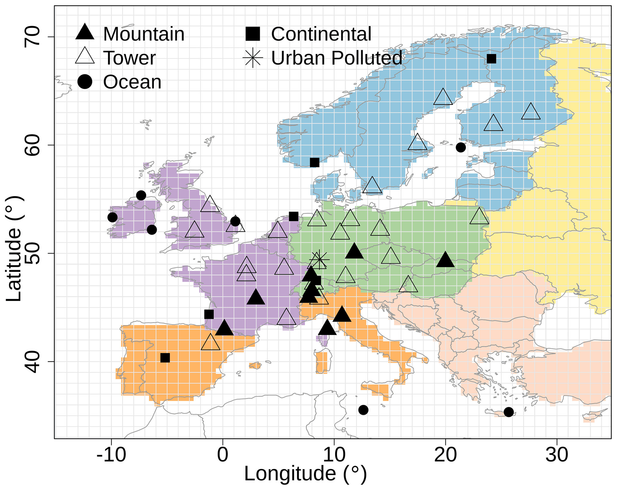
Figure 1 Station network distribution over Europe. Different graphical symbols denote the type of station classifications; coloured regions indicate Central Europe (green), Northern Europe (blue), Western Europe (purple), Southern Europe (orange), Eastern Europe (yellow), and South-eastern Europe (light red).

The representation error is assumed to be specific for different station types, which are categorised as five classes according to the ability for regional transport models to reasonably simulate the atmospheric concentration, given the variable complexity of representing the local circulation, over each station (Rödenbeck, 2005). Weekly representation errors are presented in Table 1, defining the measurement error covariance matrix in the cost function. The observations are mostly provided at an hourly frequency, especially in recent years. We also include measurements from flask sampling (mostly weekly) when available from the corresponding sites. To better represent the well-mixed boundary layer in the STILT model, we limit our analyses to measurements of 6 h daytime for all stations, i.e. 11:00 to 16:00 LT, except for mountain sites. For the latter, night-time hours (23:00 to 04:00 LT) are chosen, as mountain sites experience free-tropospheric conditions, depending on the mountain height. Particularly before establishing ICOS in 2015, the variability of station data coverage across the period of interest was rather high, underlining the sparsity of available data (Fig. 2). Since then, the site network over Europe has been markedly expanded as new stations have been installed. It should be noted that the variability in data coverage is expected to result in an inconsistency of annual flux variations. Therefore, we combined stations into three subsets: (a) the full set of stations, referred to as “all sites”, (b) a subset of 15 stations that have consistent coverage from 2006 to 2019, to which we will refer as “core sites”, and (c) a third subset of 16 stations that do not have gaps longer than 1 month during 2015–2019, subsequently referred to as “recent sites”. The far-field contributions provided to the regional domain were calculated in the two-step inversion approach (Rödenbeck et al., 2009) using a global observational record from 75 sites (https://doi.org/10.17871/CarboScope-s10oc_v2020, Rödenbeck, 2020), which has the best data coverage in the 2010–2019 period.

Table 1 Representation error of station locations.​​​​​​​

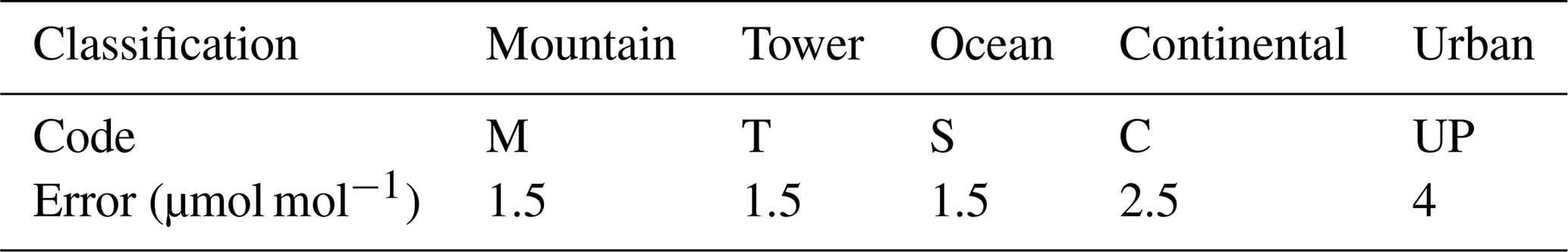
Figure 2 Dataset density measured from 2006 until 2019 over Europe. Yellow to red colour scale denotes monthly-averaged dry mole fractions of CO₂. Symbols on the right-hand axis: C – core site; R – recent site.

2.3 A priori fluxes

Terrestrial ecosystem flux models are utilised to provide prior knowledge of biogenic fluxes (NEE, defined as net ecosystem exchange). To appropriately represent the diurnal cycle in our modelling framework, NEE is obtained from the biosphere models at an hourly temporal resolution. Three biosphere models were used as priors in the inversion runs. The first is the Vegetation Photosynthesis and Respiration Model, VPRM (Mahadevan et al., 2008). VPRM is a diagnostic model driven by shortwave radiation and temperature at 2 m from the ECMWF's high-resolution operational forecast product (IFS HRES). To calculate NEE and respiration fluxes, it uses MODIS (Moderate Resolution Imaging Spectroradiometer) indices derived from surface reflectance, namely the Enhanced Vegetation Index (EVI) and land surface water index (LSWI) together with type-specific vegetation parameters optimised against the eddy covariance (EC) data. Parameter values for VPRM previously used by Kountouris et al. (2018b) were updated using the most recent EC data and are available at https://www.bgc-jena.mpg.de/bsi/index.php/Services/VPRMparam (last access: 20 October 2021​​​​​​​). The second biosphere prior is from the data-driven modelling approach FLUXCOM, which combines eddy covariance measurements and satellite observations in several machine learning algorithms to quantify the surface–atmosphere energy and carbon fluxes (Jung et al., 2020). Here, we use an extension of the modelling set-up described in Bodesheim et al. (2018), which employs daily and hourly surface meteorological information from ERA5 as well as a mean annual cycle of satellite data to produce NEE estimates at an hourly temporal and 0.5^∘ spatial resolution. It should be noted that the magnitude of interannual changes in the data-driven flux estimates is generally found to be unrealistically small (Jung et al., 2011). The terrestrial biosphere model SiBCASA (Schaefer et al., 2008) is used as the third biosphere model. SiBCASA is a combined framework based on the Simple Biosphere (SiB) model and the Carnegie–Ames–Stanford Approach (CASA) model. As explained in Schaefer et al. (2008), gross primary productivity (GPP) is calculated by SiB assuming that it is in balance with heterotrophic and autotrophic respiration (R_H, R_A), meaning that diurnal and seasonal variations are well represented; however, the long-term terrestrial carbon changes cannot be predicted by SiB component alone. CASA fills this gap as it includes a light-use-efficiency model to estimate net primary productivity (NPP, equal to GPP – R_A). In turn, CASA cannot calculate NEE during night-time. Therefore, combining both models in a hybrid version of SiBCASA combines the advantages in their biophysical and biogeochemical aspects to calculate NEE from R_H, R_A (SiB), and NPP (CASA).

Following Kountouris et al. (2018b), we assume that the spatial correlation of the prior uncertainty follows a hyperbolic decay function, similar to the inversion case nBVH (no Bias VPRM as prior with a hyperbolic decaying correlation of the spatial uncertainty structure) described in that study. In this case, the annually aggregated uncertainty matches the assumed prior uncertainty without the need for an additional bias term in the biosphere flux model. The spatial correlation length scales are 66.4 km in the zonal direction and 33.2 km in the meridional direction. One notable difference in the current work is the improved implementation of the directional dependence, with a twofold increase in decay distance in the meridional direction. Temporarily, prior uncertainties are assumed to be correlated over 30 d, as found in Kountouris et al. (2015).

Ocean CO₂ fluxes and anthropogenic emissions are regarded as prescribed fluxes in the inversion system. Ocean fluxes are taken from two sources at a coarse spatial resolution, (5 × 4^∘): a climatological flux product with monthly fluxes of Fletcher et al. (2007) and the CarboScope pCO₂-based ocean flux, providing fluxes at 6-hourly temporal resolution (Rödenbeck et al., 2013). The CarboScope pCO₂-based ocean fluxes comprise seasonal, interannual, and day-to-day variations and are updated in the CarboScope global inversion based on the Surface Ocean CO₂ Atlas pCO₂ observations (SOCAT). We have used fossil fuel emissions developed in-house based on the category and fuel-type-specific emission inventories of EDGAR-v4.3 (Emissions Database for Global Atmospheric Research), and further processed following the COFFEE approach (Steinbach et al., 2011) to include diurnal, weekly , seasonal, and annual variations. These emissions are updated annually according to national consumption data from the BP (British Petroleum) statistical review of world energy (BP Annual Report 2019) and are available from the ICOS Carbon Portal under https://doi.org/10.18160/Y9QV-S113 (Karstens, 2019)​​​​​​​. We estimate the uncertainty associated with the anthropogenic emissions for 2014 by comparing fossil fuel emissions over the EU27+UK as reported in Petrescu et al. (2021). In their study, they have reported data from eight sources, including an EDGAR product, and the spread over the annual total is 0.038 PgC with a mean of 0.974 PgC yr⁻¹, suggesting uncertainty of around 4 % among those emission products. If we assume this is also the uncertainty of our anthropogenic emission product, we can compare it to the spread of prior NEE in our study (0.940 PgC yr⁻¹). As a result, prescribing fossil fuel in the inversion and solving for NEE is appropriate; however, when interpreting posterior biosphere–atmosphere exchange fluxes, one has to take into account that part of the fluxes and their variability might be compensating for errors in anthropogenic emissions.

2.4 Set-up of the inversion runs

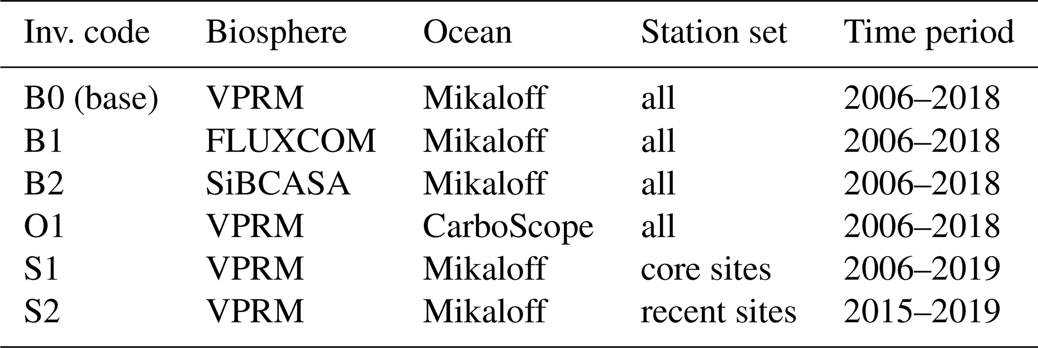
We conduct three ensembles of inversion runs listed in Table 2 utilising different set-ups of prior products (biosphere and ocean ensembles) as well as selected sets of observational data (station set ensemble). The inversion runs are labelled with unique codes for reference. B0 is defined as the base case of our analysis. It is configured using default settings of the inversion runs, with biogenic fluxes from VPRM and climatological ocean fluxes, and using all available atmospheric data as input. In the biosphere ensemble (consisting of B0, B1, and B2), FLUXCOM and SiBCASA replace the VPRM model in both B1 and B2, respectively, allowing for a distinction between the effect of using different prior flux models on posterior NEE. This ensemble of inversions was performed for the period 2006–2018, as the availability of SiBCASA fluxes was limited to this period of time. In the ocean ensemble, we replace the climatological ocean fluxes used in B0 with the pCO₂-based CarboScope ocean fluxes in O1. The station set ensemble is formed by running the inversion with varying measurement station subsets as explained in Sect. 2.2: B0 – all sites; S1 – core sites; and S2 – recent sites. For each of the three ensembles of inversions, its spread is calculated as the standard deviation of the differences between each ensemble member and the ensemble mean over the respective overlapping period of time. The statistical uncertainty is calculated in the inverse system based on model–data mismatch and the prescribed prior uncertainty and was performed for the base case inversion (B0) as it remains identical independent of the biosphere model used.

Table 2 Set-ups of the inversions.

3 Results

3.1 Statistical analysis of ensemble uncertainties

The annual NEE estimates among the biosphere ensemble (Fig. 3) show good agreement across the three biosphere models but also across S1 and O1 inversions, yielding similar budgets of CO₂ fluxes over the full domain. The findings suggest that atmospheric data constraints are more dominated in the posterior NEE fluxes in comparison with the prior constraint. Subregions that are characterised by strong observational constraints such as Central Europe show a closer consistency in the posterior fluxes despite large prior differences among the biosphere models compared to the regions less constrained by atmospheric data, such as Northern Europe.

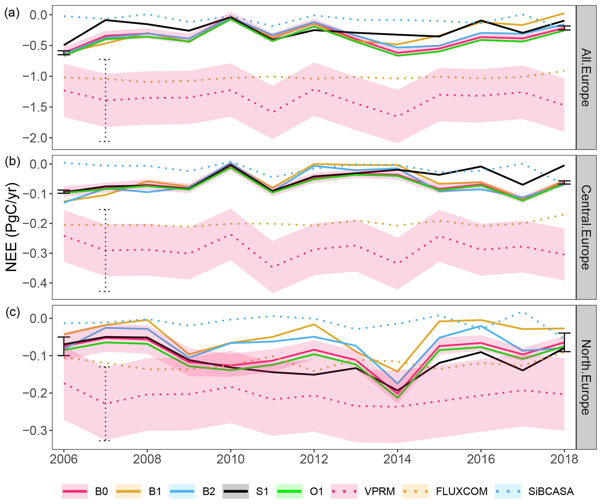
Figure 3 NEE fluxes estimated using B0, B1, B2, S1, and O1 inversions for the 2006–2018 period over the full domain of Europe (a), Central Europe (b), and Northern Europe (c). Posterior fluxes are plotted with solid lines and their a priori fluxes as the dotted lines. Priors and posteriors of the biogenic ensemble are distinguished by identical colours for each modelled scenario. Light red shadowing denotes the statistical uncertainty and error bars indicate the spread among the biosphere inversions' ensemble.

It is noteworthy that there is a striking similarity in interannual variations between the a posteriori fluxes and both VPRM and SiBCASA prior fluxes for the years 2009–2013. This agreement does not necessarily mean that posterior interannual variability (IAV) is driven by biosphere models. This can be deduced from B1 (FLUXCOM) estimates from which the IAV differs in both the prior and posterior fluxes and where FLUXCOM NEE has weak interannual variations. Instead, VPRM and SiBCASA are likely to import this signal from the meteorological data used to force these models. However, the VPRM model overestimates the mean CO₂ uptake compared to the a posteriori fluxes, while SiBCASA underestimates the mean CO₂ uptake, and this dissimilarity is persistent for all years as well.

The statistical uncertainty and spreads over the ensembles are evaluated and affect our data (Fig. 3). It is noticed that the spreads over the posterior fluxes and prior fluxes are comparable with the corresponding uncertainties over the full domain (All Europe), Central Europe, and Northern Europe. Note that calculating the spread over a small size of samples might not reflect the true standard deviation. There is a clear reduction in uncertainty and spread in posterior fluxes either over the full domain (All Europe) or in subregions like Central and Northern Europe. Unlike prior uncertainty, posterior uncertainty slightly differs from year to year following the number of atmospheric sites available (Fig. 2). This gets even clearer when looking at the marked reduction in the posterior uncertainty in Central Europe as well as in regions with high station density, resulting in a stronger observational constraint. In contrast to Central Europe, a smaller reduction in posterior spread is found in Northern Europe as well as in other regions where there are few or no stations (e.g. Eastern Europe, Fig. S1 in the Supplement). In this case, NEE estimates are not well constrained by atmospheric data. Instead, a posteriori flux is driven by the inversion using biosphere models and their uncertainty, particularly for the distant areas that cannot be constrained by observations through the spatial correlation. Table 3 denotes the reduction in the biosphere ensemble spread in the a posteriori spread relative to the a priori spread over the full domain, Central and Northern Europe (95.1 %, 96.0 %, and 74.8 %, respectively). It indicates less reduction in Northern Europe due to the sparseness of observational sites. The large reduction in spread in Central Europe reflects a notable dependency of NEE estimates on the atmospheric measurements, substantially where the observation network is dense.

Table 3 Reduction in the biosphere ensemble NEE spread over Europe.

To analyse the seasonal variations, the seasonal cycle from B0, B1, B2, S1, and O1 inversions is averaged over 13 years for the full domain of Europe together with the corresponding biogenic prior fluxes for VPRM, FLUXCOM, and SiBCASA (Fig. 4). Results show good agreement amid a posteriori results of all inversions, while prior biosphere models show large differences, a pattern similar to the one seen over the annual fluxes in Fig. 3. Nevertheless, posterior NEE fluxes estimated in the S1​​​​​​​ inversion show differences during May–August when compared with the estimates of other runs, reflecting a larger sensitivity of IAV to summer fluxes when applying a different set of stations. In addition, the difference in posterior fluxes seen in Fig. 3 over the annually aggregated estimates computed from the B1 inversion over the period 2014–2018 largely results from the estimates during May and June when comparing them to the rest of biosphere ensemble elements (Fig. 4).

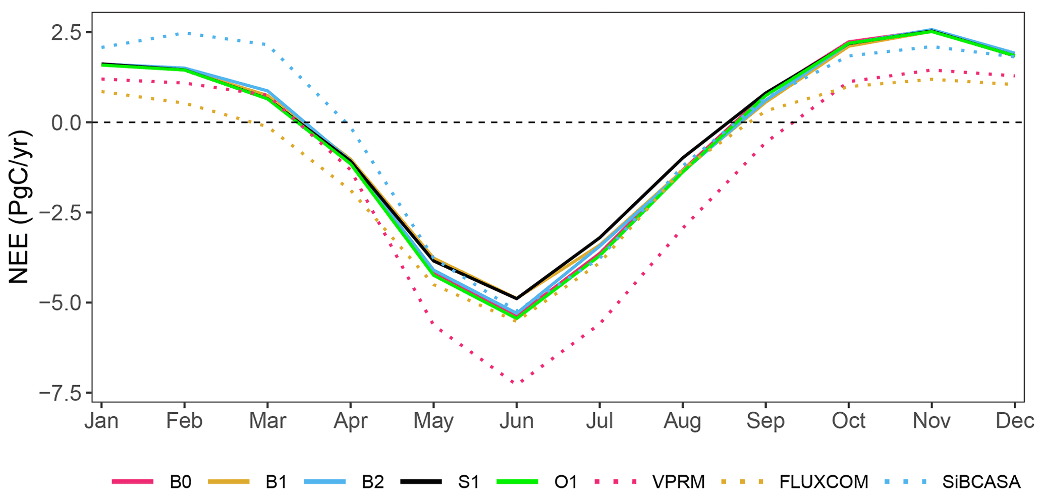
Figure 4 Seasonal cycle of NEE calculated as the average of monthly fluxes over 13 years estimated using the ensembles of inversions (solid lines) B0, B1, B2, S1, and O1 as well as the biogenic prior fluxes (dotted lines) obtained from VPRM, FLUXCOM, and SiBCASA.

Figure 5 illustrates the statistical uncertainty and the spread through the overall ensembles of inversions (listed in Table 2) calculated annually over three regions. As was discussed in the time series of NEE (Fig. 3), a reduction in posterior NEE uncertainty with respect to the assumed prior uncertainty is clear (dark grey bars in Fig. 5). A larger reduction is realised in Central Europe, emphasising a strong atmospheric signal constraint in the inversion. The spread among ensemble members (Fig. 5, yellow bars) represents the standard deviation of the respective inversion results. The ensemble spread over the a priori biosphere models agrees with the assumed prior uncertainty, with a relatively high value (about 0.44 PgC yr⁻¹ domain-wide) indicating large discrepancies between prior flux models. This confirms that the prior uncertainty assumed in the CSR system is realistic. The IAV of B0 was calculated separately for prior and posterior fluxes (blue bars) from the anomalies relative to the long-term mean to reveal the magnitudes of interannual deviation in comparison with the spread variability.

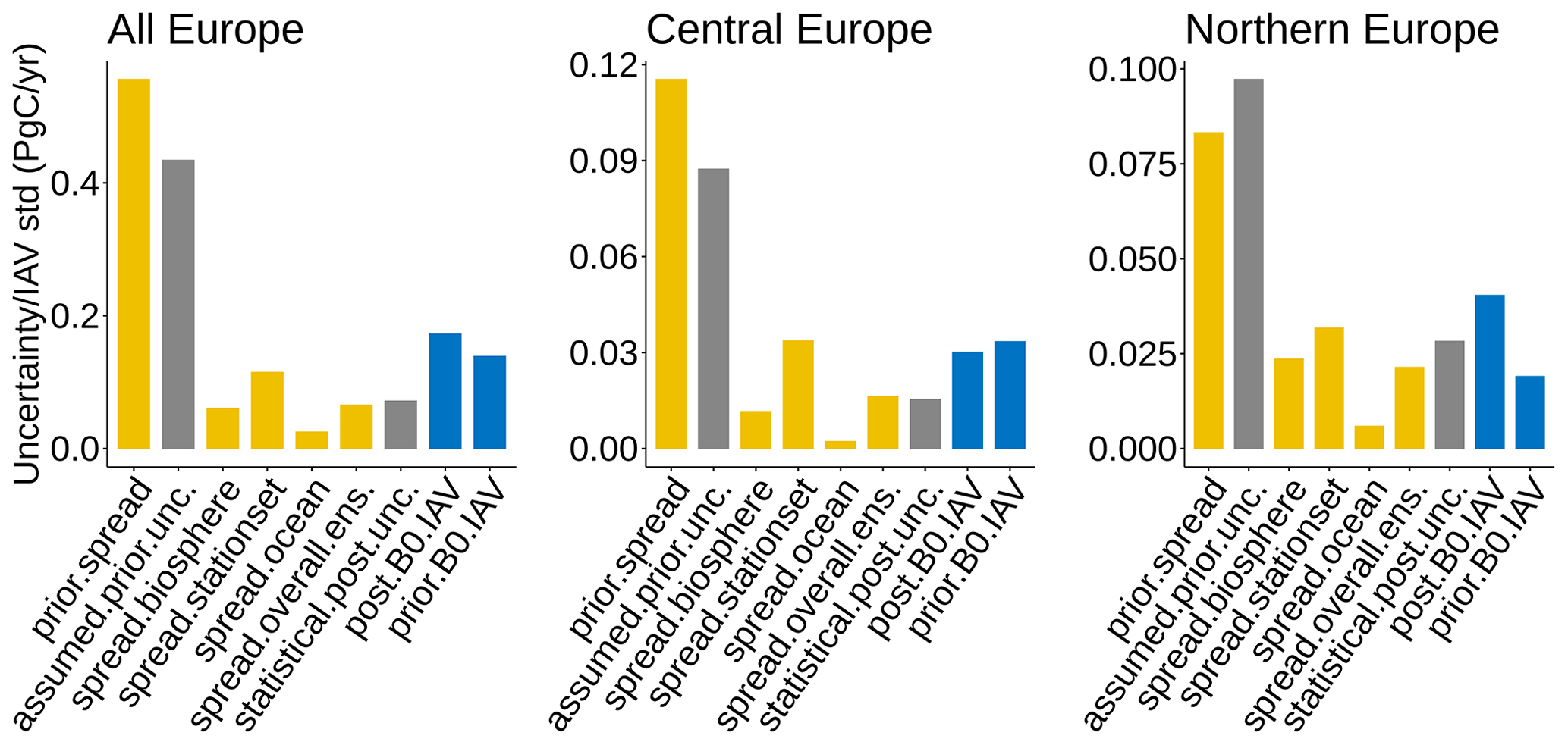
Figure 5 Spread uncertainties calculated from three inversion ensembles of biosphere, ocean, and station set (yellow bars). Grey bars refer to the statistical uncertainties, and blue bars denote the standard deviations of IAV.

In terms of the spread of the biosphere ensemble, the standard deviation of posterior fluxes declines from 0.666 to 0.032 PgC yr⁻¹ over All Europe. Spatial differences are expected as stations are not evenly distributed across the domain of Europe. This can be noticed from the spread over Central Europe (a large number of stations, 18 sites) and Northern Europe (a smaller number of stations, 8 sites). As a result, the lack of observations leads to inflating the spread over the biosphere ensembles.

The largest impact on NEE estimates in the ensembles is observed when the spread over the station set ensemble is analysed. In this regard, a robust analysis can be based on a subset from Central Europe, as the subsets of stations in this region clearly contrast in the two ensemble members (core sites and recent sites). The spread of the station set ensemble was found to be 0.11 PgC yr⁻¹ – larger than those resulting from the biosphere and ocean ensembles (0.05 and 0.02 PgC yr⁻¹, respectively). It is noteworthy that the spread in the station set ensemble is slightly larger than the statistical uncertainty, highlighting the importance of performing ensembles of inversions using different numbers of stations to assess the posterior uncertainty. In addition, NEE estimated among the station set ensemble suggests that while in all cases the posterior fluxes are data-driven, modification of the observation inputs leads to interannual variations. The spread of the ocean ensemble remains the smallest in all the regions, indicating quite a weak dependency of posterior NEE estimates on ocean fluxes, in particular over inland regions (e.g. Central Europe).

The spatially distributed spread of all ensembles is depicted in Fig. 6. In this instance, the standard deviation was calculated for each grid cell rather than aggregating fluxes over regions first and then computing the spread (Fig. 5). The spatial spread here illustrates the deviations in the biosphere ensemble (“Biosphere spread”), the biosphere models (“Prior biosphere spread”), the station set ensemble (“Stationset spread”), and the ocean ensemble (“Ocean spread”). The maximum spread of 0.191 × 10⁻⁴ (PgC yr⁻¹) was observed over the a priori terrestrial biosphere models, particularly concentrated in Central and Southern Europe. The spread of the a posteriori biosphere ensemble is significantly reduced. In the station set ensemble, isolated stations like Hegyhátsál in Hungary and Sierra de Gredos in Spain demonstrate a relatively high impact on the NEE spatial patterns over broader areas, reflecting the inversion correlation length. However, such an impact is not clearly realised in the Stationset spread map amid dense clusters of sites due to the commutative constraint that compensates for the excluded sites within the subsets of stations. These results highlight the importance of defining a proper function of spatial correlation decay in the prior uncertainty structure. Quite a small influence is seen through the spread over the ocean, where a slight impact emerges only in wider coastal regions, being almost negligible inland (e.g. in Central and Eastern Europe).

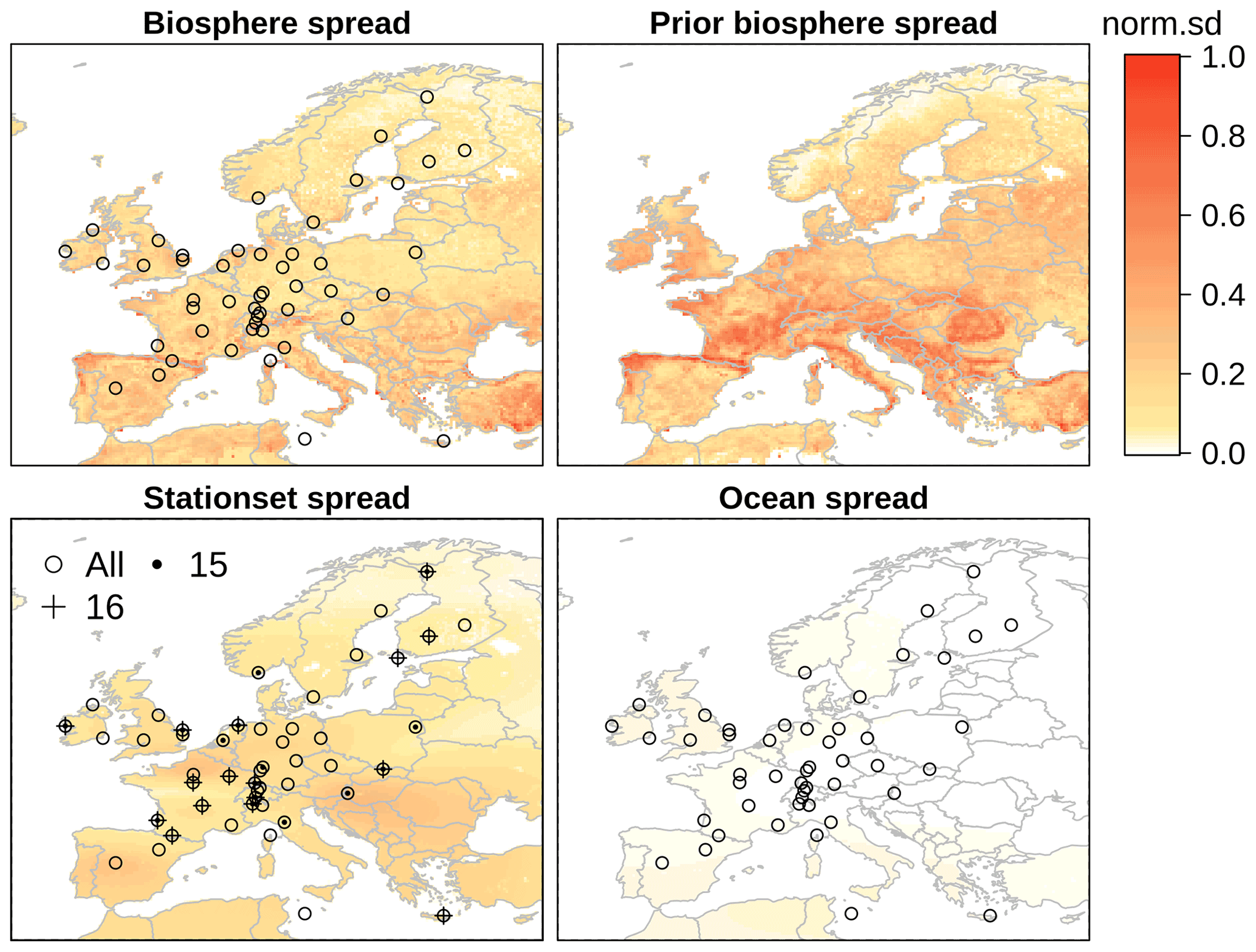
Figure 6 Spatial spread of biosphere, prior, station set, and ocean ensembles. Standard deviation (SD) in the legend is normalised over maximum spread 1.91 × 10⁻⁴ in units of PgC yr⁻¹ per grid pixel. Stations used in the station set ensemble are referred to by circles (B0), dots (S1), and the plus symbol (S2).

Figure 7 indicates the spatial distributions of prior and posterior NEE averaged over the full 13-year period, estimated from B0, B1, and B2 inversions as well as the corresponding innovation of fluxes (the difference between posterior and prior fluxes). Positive corrections have been made to the biosphere flux models that are regarded to be negatively biased (VPRM and FLUXCOM, as was unequivocally confirmed by the annual time series of NEE in Fig. 3). In contrast, SiBCASA results are closer to the mean of posterior fluxes, with a small domain-wide negative correction, except for local positive innovations seen over Northern Germany and the Western Mediterranean coast.

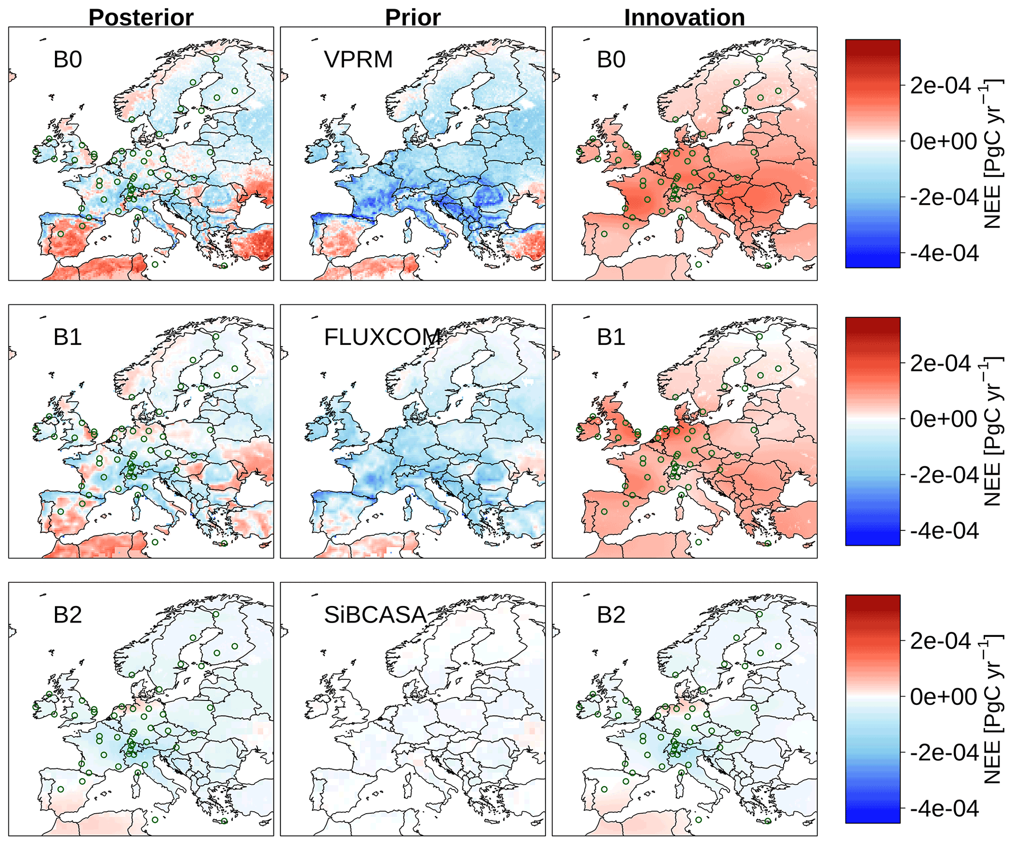
Figure 7 Posterior, prior, and innovation of fluxes (posterior – prior) averaged over the 2006–2018 period calculated from the biosphere ensemble of inversions (B0, B1, and B2). Green circles refer to observing sites.

3.2 NEE estimates of 2018 and 2019 in a pre-operational system

In this section, we present CO₂ fluxes for 2 selected years estimated in a pre-operational system in the context of long-term estimates. In synergy with the research project VERIFY in alignment with the scope of the Paris Climate Agreement, the system is used to provide annual updates of estimated fluxes over Europe once the atmospheric observations and auxiliary data required to force prior flux models and atmospheric transport models are available. The CSR is described as a “pre-operational system”, as it is still under development from year to year. The period of interest is chosen to start from 2006, in which a better coverage of observations exists within the domain of Europe. Here, we give special attention to analysis of the drivers of spatiotemporal differences in line with climate disturbances that occurred in 2018 and 2019, during which inaccuracies of estimating the continental fluxes of CO₂ have been reported (Friedlingstein et al., 2019). This is due to the sensitivity of ecosystem respiration and photosynthetic fluxes to extreme events like lasting droughts. The analysis here is based on two inversion runs using observational data only from the subset of core sites that have consistent measurements, i.e. (1) the S1 inversion set-up and (2) a similar set-up to S1 performed with FLUXCOM instead of VPRM. The choice of using consistent measurements is essential to study the IAV to diminish the uncertainty caused by gaps of data coverage over years. The IAV of estimated CO₂ fluxes is then compared with the IAV of the biosphere flux models (VPRM and FLUXCOM) used as priors in the two inversion runs.

Summer NEE anomalies between 2006 and 2019 (ΔNEE, Fig. 8) are positive in the years 2007, 2010, 2016, 2018, and 2019 indicating that the mean uptake of CO₂ during the growing season was lower than average in these years. The magnitudes of anomalies during these years are comparable with findings of NEE anomalies reported by Rödenbeck et al. (2020) but estimated using different global inversion runs (2019 was not included in that study). Herein, we shed more light on 2019 NEE estimates which suggest an even weaker uptake of CO₂ in comparison with the summer of 2018. It is noticed that the posterior fluxes estimated using the biosphere model FLUXCOM exhibit the largest anomaly of NEE during the summer of 2019. Despite slight differences in the amplitude of IAV, there is good agreement in the posterior fluxes estimated with both the FLUXCOM and VPRM models. Such common agreement is inherited from the identical observations used in both the inversion runs, as demonstrated in the case of the biosphere ensemble in Sect. 3.1. Therefore, the IAV in this case is more likely to be attributed to climate anomalies, in particular during drought occurrence in the growing season.

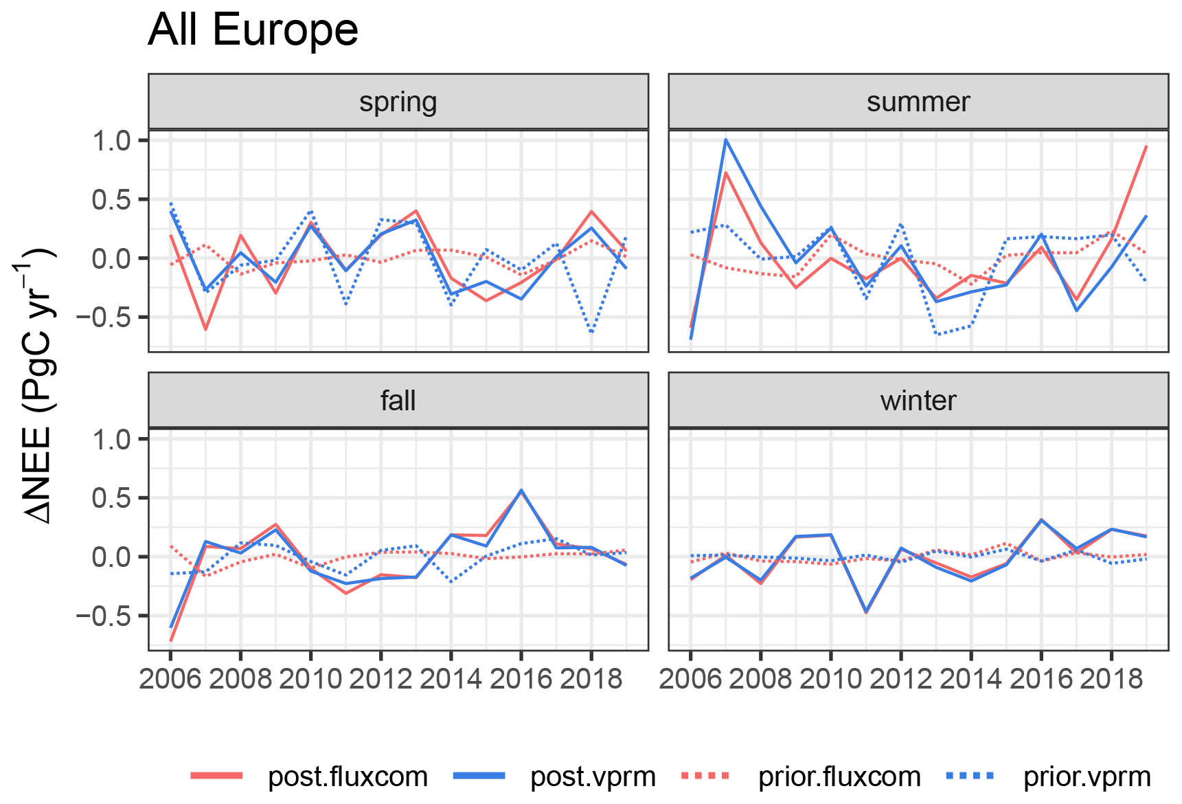
Figure 8 Anomalies of NEE fluxes during spring, summer, fall, and winter estimated from two inversion runs differing in biosphere models (FLUXCOM in red colour and VPRM in blue colour) using the atmospheric data of core sites. Solid lines indicate the a posteriori anomalies, while dashed lines refer to the corresponding a priori (biosphere models) anomalies.

The agreement between posterior fluxes using FLUXCOM and prior fluxes of VPRM in the spring season confirms two important conjectures: (1) posterior IAV are largely derived by atmospheric data regardless of the biosphere model used; (2) the VPRM model can capture year-to-year variations during spring, reflecting its capability to represent dynamic biospheric activity during the growing season. It is clear that FLUXCOM exhibits remarkably weaker annual variations during spring and fall in comparison with the VPRM and the a posteriori fluxes. In winter, the VPRM model agrees well with FLUXCOM in the interannual variations, showing less IAV compared to the NEE estimates. We attribute this to the lower signal of temperature assimilated in the biosphere models from the meteorological data as well as less information of radiation reflectance obtained from the remote-sensing data due to dominant cloudy scenes in winter, provided that the VPRM and FLUXCOM models use forcing data from meteorology and remote sensing. In addition, misrepresentation in the anthropogenic emissions prescribed in the inversion may contribute to the posterior IAV, in particular during winter due to the fact that the biosphere signal is generally weak.

To assess the temporal changes in NEE in response to such climate variations, we compare the seasonal anomalies of NEE (prior and posterior) to the anomalies of 2 m air temperature and Standardised Precipitation–Evapotranspiration Index (SPEI) (Beguería et al., 2014) during spring, summer, fall, and winter as well as the annual mean (Fig. 9). Here we show estimated NEE integrated over the full domain. Monthly near-real-time data of SPEI (SPEI01) are obtained from https://spei.csic.es/map/maps.html (last access: 24 December 2020​​​​​​​) at 1^∘ spatial resolution and monthly 2 m air temperature accessed via https://psl.noaa.gov/data/gridded/index.html (last access: 11 February 2021​​​​​​​) at 0.5^∘​​​​​​​ spatial resolution. The anomalies were normalised with the standard deviation of the interannual variations since 2006. In addition, Pearson correlation coefficients between posterior fluxes, prior fluxes, temperature, and SPEI for the full year and calendar seasons were calculated. It is of note that, due to the fact that the biosphere model VPRM utilises temperature from meteorological fields and EVI data from the satellite sensor MODIS, it is anticipated to systematically correlate with temperature and SPEI. Consequently, we mostly devote our comparison to the posterior fluxes.

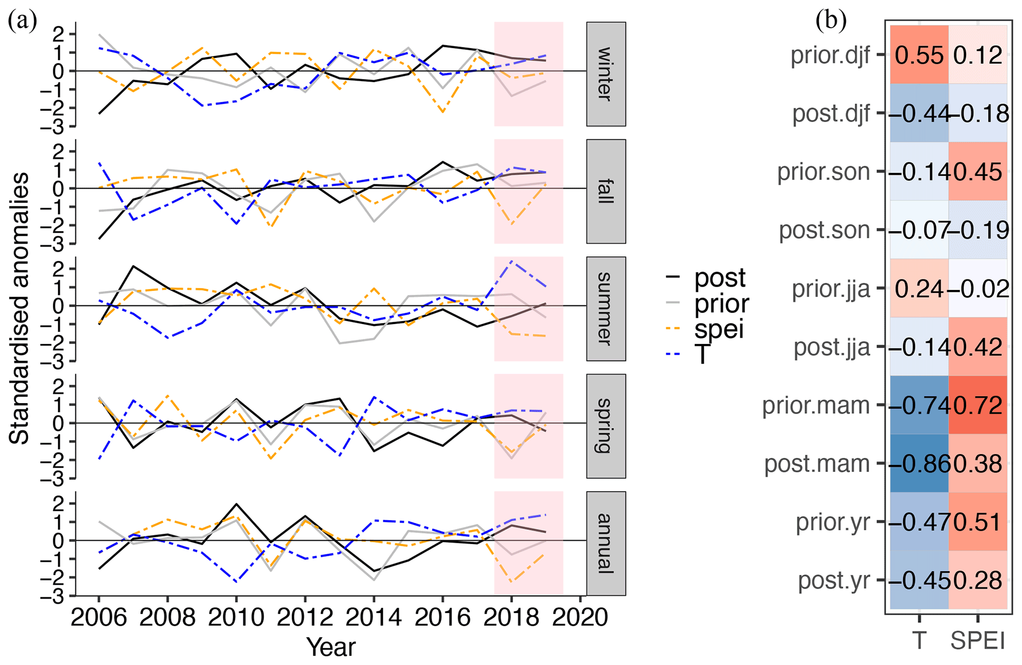
Figure 9 Panel (a) shows the anomalies of posterior NEE (post), prior NEE (prior), SPEI (spei), and 2 m air temperature (T) standardised relative to the standard deviation of climatological variations at annual and seasonal scales since 2006 over the full domain of Europe. Units of NEE and temperature are in PgC yr⁻¹ and K, respectively, while SPEI is unitless. Panel (b) refers to the correlation coefficients of posterior and prior NEE on the y axis with SPEI and air temperature on the x axis calculated in springs (mam), summers (jja), falls (son), and winters (djf) and at annual scales (yr) over the full domain of Europe. Note: seasonal T and SPEI correspond to NEE seasons mentioned on the y axis.

The findings of standardised anomalies in Fig. 9a show that the decrease in CO₂ uptake in 2018 and 2019 during the growing season was concurrent with a profound deficit of soil water content (SWC) (negative SPEI anomalies, dry conditions). The reduction or very low SWC also coincided with an unprecedented rise in temperature (positive T anomalies, highest in 2018) across Europe. Being an indicative factor of drought occurrences, SPEI links water availability in the surface including soil moisture (crucial limitation of GPP, especially in the temperate regions) and temperature to the precipitation and evapotranspiration rate. Hence, there is quite good agreement between posterior NEE and SPEI not only at spatial scales but also at temporal scales. The standard deviations of the interannual variations in posterior NEE, SPEI, and temperature over All Europe in the annual mean through the 14 years were equal to 0.17 PgC yr⁻¹, 0.12, and 0.45 K, respectively. When relating the changes occurring during 2018 and 2019 to the context of the previous 12 years, the annual anomalies of SPEI were found to decline to more than twice as much as the climatological deviation: around −0.29 in 2018 and to around −0.08 in 2019. As a consequence, posterior NEE anomalies increased to 0.14 and 0.08 PgC yr⁻¹ above the climatological mean in 2018 and 2019, respectively.

The excess of annually averaged temperature was predominant in 2018 and 2019, reaching around 0.40 and 0.47 ^∘C above the climatological mean, respectively. Despite the fact that the impact of the 2018 and 2019 drought on NEE is realised from the SPEI and temperature anomalies, there is a relatively moderate correlation between estimated NEE and SPEI and temperature at the annual scale over the full domain (Fig. 9b). However, the correlation coefficients vary greatly between seasons. A high anticorrelation (−0.86) between estimated NEE and temperature is found to be consistent during spring. In contrast, anticorrelation drastically decreases and turns out to almost vanish in summer and fall. Nonetheless, the relatively moderate correlation of SPEI with posterior NEE during summer is adequate to deduce the lack of SWC under dry conditions through the anticorrelation between SPEI and temperature. This implies that warm conditions accelerate the depletion of soil moisture content, in particular in the soil top layer that lacks water content in its deeper layers to compensate for the higher evaporation rate at the surface layer. This affects photosynthesis efficiency during the growing season by decreasing the gross primary productivity but also increases the contribution of soil respiration, which is more pronounced in 2019.

During winter, water availability does not seem to be a limiting factor of NEE as we notice from low correlations between posterior NEE and SPEI. Instead, temperature negatively correlates with posterior NEE indicating that the increase in temperature coincides with enhanced uptake of CO₂ where photosynthesis can occur, e.g. in evergreen areas. But cold years have more and longer snow cover which decreases photosynthesis, whereas soil heterotrophic respiration contributes more to CO₂ release since soil temperature is expected to be larger than air temperature owing to snow cover insulation. Meanwhile, the anticorrelations between estimated NEE and temperature may result from a misattribution of anthropogenic emissions, as warmer winters mean less anthropogenic emissions (the opposite holds true for colder winters). It is of note that X December, X+1 January, and X+1 February are incorporated into the winter estimate of a specific year (X). Figure 10 illustrates the seasonal contribution of NEE to IAV, which is dominated by summer and spring variability in comparison with winter. We note that the posterior fluxes are in agreement with the biosphere model VPRM in summer and fall, while the variability of posterior fluxes is larger during winter and smaller during spring compared to prior fluxes; the opposite holds true for the prior fluxes. Temperature is, however, shown to vary greatly during winter, while the SPEI contribution does not show a significant variability between seasons.

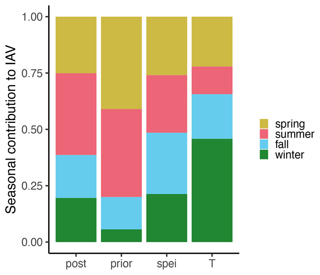
Figure 10 Seasonal contribution to IAV calculated relative to 14 years for posterior NEE fluxes (post), VPRM NEE fluxes (prior), SPEI, and T during the four seasons over the full domain.

3.2.1 Spatial differences in NEE estimates in 2018 and 2019

Using an identical set of observation sites for the last 5 years, the S2 inversion demonstrates the differences between NEE estimates in 2018 and 2019 as seen in Fig. 11. Results emphasise the aftermath of drought episodes, showing a smaller uptake of CO₂ in France, Germany, and Northern Europe during the spring of 2018 (March–April–May), while during the summer of 2019 (June–July–August) the estimates of NEE, to some extent, suggest a higher CO₂ release, in particular in the United Kingdom, France, Germany, and Southern Europe. NEE estimates during the fall of 2018 suggest less uptake in Western, Northern, and Southern Europe compared to the fall of 2019. Obviously, during winter time (December–January–February) the differences are infinitesimally small throughout the full domain, while the annual mean fluxes indicate much smaller uptake in 2018 compared to 2019. This confirms a longer impact of the drought lasting from the early growing season during spring until the end of summer. To explain the changes in spatial distribution of NEE alongside SPEI and temperature in 2019, anomalies of NEE were estimated using the S1 inversion with respect to 2006–2018 anomalies. Figure 12 indicates the coincidence of the large release of CO₂ during summer time in Central Europe with the positive anomalies of temperature and the negative anomalies of SPEI over those regions. The prior fluxes, to a lesser extent, show the impact of temperature and SWC on NEE during the growing season. However, in the United Kingdom positive NEE anomalies can only be detected from the posterior fluxes. The positive anomalies of temperature during winter show a slight impact on NEE (positive anomalies). This can be interpreted as an increase in soil respiration.

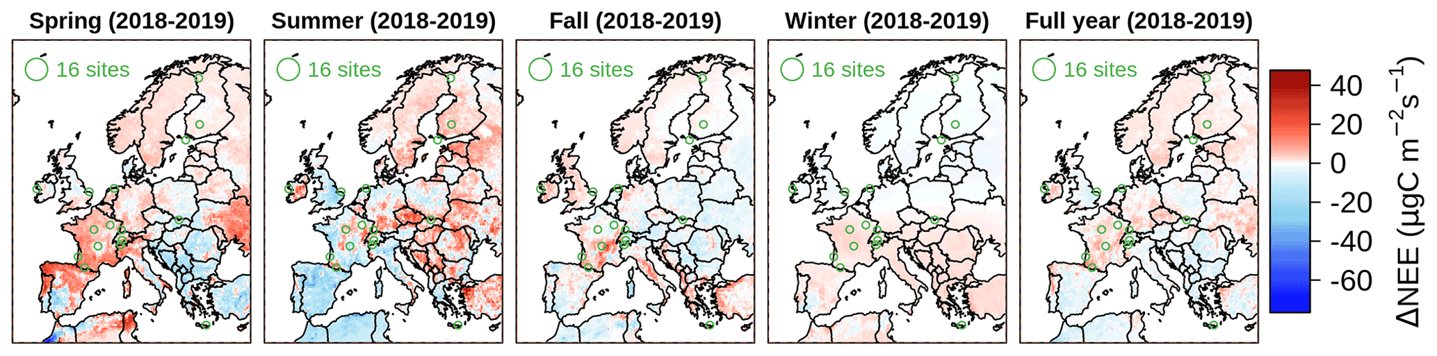
Figure 11 Differences in NEE estimates for 2018–2019 in seasonal and annual mean calculated from the S2 inversion set-up.

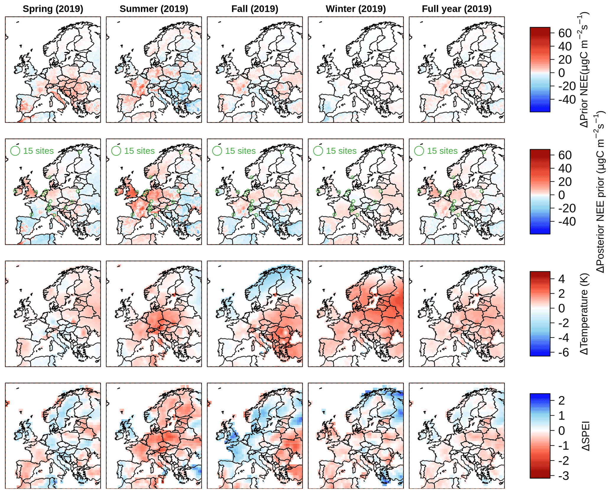
Figure 12 The 2019 anomalies of prior fluxes (first row), posterior NEE estimated from the S1 inversion (second row), 2 m air temperature (third row), and SPEI (fourth row) relative to 2006–2019 over Europe. Columns denote mean estimates of spring, summer, fall, winter, and annual NEE estimates, from left to right.

The annual budgets of NEE in 2019 and 2018 are summarised in Fig. 13 for six subregions estimated using the B0 and S2 inversions. The choice to use the B0 inversion is to estimate annual flux budgets of CO₂ through assimilating as many atmospheric observations as possible to strengthen the observational constraint in the spatial and temporal aspects. The S2 inversion is specifically used to keep identical observations in 2018 and 2019 for the purpose of assessing the NEE differences between the 2 years. The annually aggregated fluxes estimated from the B0 inversion over the full domain yield −0.28 and −0.22 PgC in 2019 and 2018, respectively. The performance of the inversion reflected in the a posteriori fluxes is associated with an uncertainty reduction of 85.5 to 88 % with respect to assumed prior uncertainty for 2019 and 2018, respectively. Likewise, the underlying European regions indicate an uncertainty reduction with different magnitudes based on atmospheric data availability. The relatively observationally weak constraint in 2019 has thus resulted in a small increment of posterior uncertainty in regions that have a smaller number of stations. For instance, the uncertainty in Southern Europe was amplified from 0.018 PgC in 2018 to 0.027 PgC in 2019, coinciding with an increase in the net source of CO₂ fluxes from 0.016 in 2018 to 0.069 PgC in 2019. Despite the data coverage difference in both years, Southern Europe still shows a larger annual flux of 0.04 PgC in 2019 estimated using the S2 inversion in comparison with 0.02 PgC in 2018.

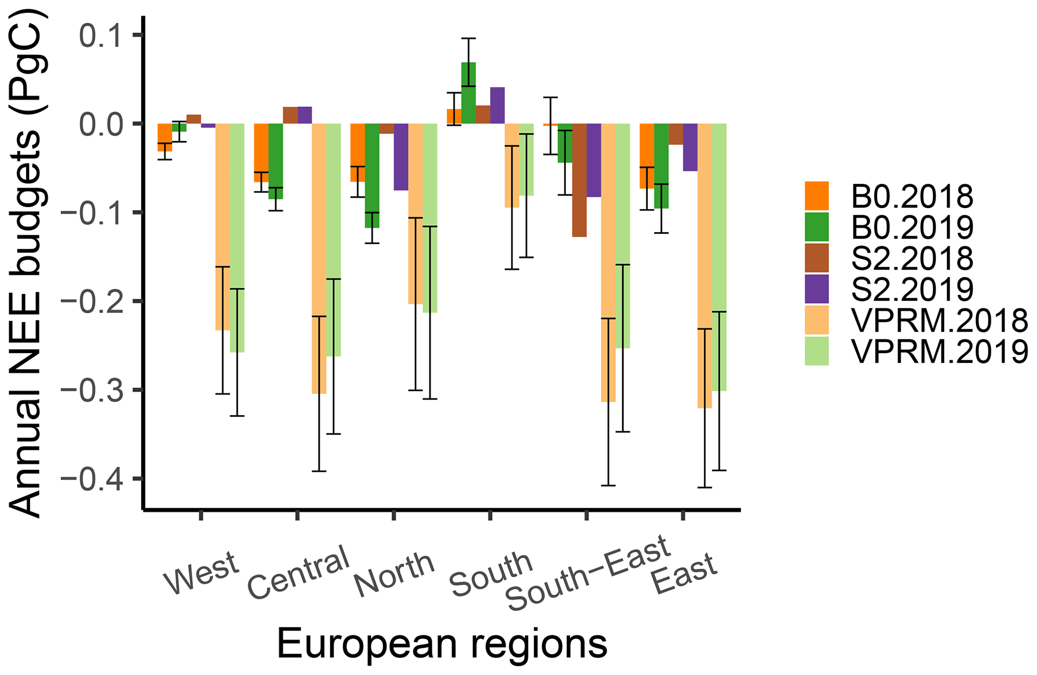
Figure 13 Posterior NEE flux budgets over six European regions in 2018 and 2019 using the B0 and S2 inversions (dark colours) compared to their priors from the VPRM model (light colours). Uncertainties associated with B0 and VPRM fluxes are referred to in the error bars.

These results, again, highlight the sensitivity of the inversion to data coverage but also the stronger impact of warmer summers on NEE, where S2 estimates suggest larger flux budgets in 2019 compared to 2018 over Western and Southern Europe. Overall, B0 and S2 results suggest a suppression of GPP, predominantly in Central and Northern Europe.

4 Discussion and conclusions

4.1 Sensitivity of posterior fluxes to input data

The smaller spread in the a posteriori fluxes found through the ensembles of inversions is evident over All Europe reflecting the good performance of the inversion system. In the biosphere ensemble, flux estimates are not very sensitive to a priori terrestrial ecosystem fluxes. We deduce this from the small spread over the a posteriori fluxes (Fig. 3), occurring despite major differences in a priori fluxes. Likewise, different ocean flux models have the smallest effect on estimating NEE, in particular inland, where the ocean–land exchange is dissipated. However, the spread in the station set ensemble is strongest, at 0.11 PgC yr⁻¹ for the annually aggregated fluxes over the full domain. This points out a higher sensitivity of the inversion to the number of stations in comparison with 0.06 and 0.02 PgC yr⁻¹ spreads in the biosphere and ocean ensembles, respectively. This effect is most pronounced over Central Europe, where measurements of CO₂ dry mole fractions are available from a large number of stations, and thus a contrasting number of sites manifests itself amongst station subsets, given that the station subsets were not selected based on geographical locations but on the long record of data coverage. Further, this finding corroborates the dominant influence of observational constraint on NEE estimates in the biosphere and ocean ensembles seen through interannual variations. Such influence is, however, subject to the availability of the atmospheric data which can otherwise be altered by the prior constraint to maintain the posterior estimates according to Bayes' approach. For example, the relative spread over biosphere ensembles in Northern Europe, having less dense coverage, increases to 38.4 % compared to 23.9 % in Central Europe. Conversely, in the station set ensemble, the spread calculated for Northern Europe was found to be smaller than that in Central Europe (51.8 % versus 71.7 %), reflecting the biogenic flux constraints in this case, given the smaller differences in observations among the station subsets in this ensemble. The ocean ensemble spread remains at a minimum percentage in both regions, although it is elevated to 9.6 % in Northern Europe in comparison with only 4.3 % in Central Europe. Although the impact of ocean fluxes on NEE estimates can be negligible over the full domain and inland, the results point to a relatively higher influence in the coastal regions.

Our results denote a comparable reduction in posterior uncertainty and the spread relative to their a priori (Fig. 5). It is noteworthy that the indirect effect of statistical posterior uncertainty on the corresponding spread over the ensembles of inversions emerges from the common dependency on observational data, which predominantly appear in the well-constrained areas in Germany, France, Benelux, and the UK. Over such regions, the posterior uncertainty and spreads are greatly reduced and the inversions tend to converge regardless of which prior flux model is used. It is essential to consider the prior uncertainty assumption as well as the prior error structure in the spatial and temporal aspects. This will determine to which extent the posterior fluxes are dependent on the uncertainty biogenic fluxes, specifically in the regional inversions where the degrees of freedom can drastically increase following the finer spatial and temporal resolution of biosphere flux models and atmospheric transport models.

4.2 Response of NEE estimates to climate variation

The linkage between NEE and climate variation has been examined via SPEI and temperature as proxy data of climate variation. The anomalies of SPEI and temperature are analysed along with NEE anomalies during the recent years 2018 and 2019 in the context of the period 2006–2017. The recent drought events decreased the efficiency of GPP, in particular during spring and summer, where soil moisture markedly declined during the summer of 2018 and 2019 accompanied with an exceptional rise in temperature (Ma et al., 2020). But GPP during spring 2019 showed a higher efficiency (larger uptake of CO₂) than the spring of 2018, benefiting from the increment of temperature, SWC, and light availability. The finding is consistent with a study on seasonal NEE over North America implemented by Hu et al. (2019) and seems to hold for Northern regions where temperature is substantially regarded as a limiting factor to NEE. Additionally, our results showed that Central Europe experienced higher sources of CO₂ during 2019, which can be impacted by an extended legacy of the drought of 2018, where forests were profoundly stressed and thus their growth was negatively impacted. MacKay et al. (2012) found an about 17 % reduction in drought plot growth relative to a reference plot and showed that growth reduction in the forests across Europe exceeded this value under drought conditions depending on tree species. Furthermore, the ecosystem respiration response to the temperature increment may contribute to such a positive anomaly, given that temperature anomalies during 2019 over Central and Southern Europe were unprecedented, in line with the 2018 anomaly (Hari et al., 2020). In agreement with Rödenbeck et al. (2020), we found that summer NEE anomalies were in agreement with the anomalies of temperature and SPEI, occurring in different summers including 2018.

In terms of estimated winter fluxes, the medium anticorrelation between temperature and NEE (also shown by the anomalies in Fig. 9a) may imply that an increase in CO₂ release occurs in cold winters if thicker and lasting snow cover prevails. Snow insulation prevents the soil temperatures from decreasing as strongly as air temperature. In comparatively warmer soils respiratory carbon dioxide emissions by the soil biota are sustained also during winter. In agreement with our results, Monson et al. (2006) found that soil temperature during winter increases nonlinearly with the depth of snowpack resulting in the enhancement of soil respiration. Even though the study was carried out at site level in the Northern Hemisphere in the US, the agreement with our findings indicates to a similar impact at a wide scale.

Besides the previous explanation of T-NEE anticorrelation in winter, one should take into account a hypothesis of the vertical mixing height being systematically biased in the atmospheric transport models (Lin and Gerbig, 2005). In this case, a misrepresentation of mixing height during colder winters might occur, as was demonstrated in a study conducted by Gerbig et al. (2008) devoted to characterising the uncertainty of atmospheric transport models resulting from vertical mixing changes during daytime and night-time. Given this, the shallow boundary layer developed during night holds similar characteristics during cold winters. A separate study is required to investigate such an impact, which will lead to improving vertical mixing in the atmospheric transport models and thus reducing the uncertainty in atmospheric tracer inversions. Apart from that, the contribution of winter fluxes to the interannual variations is lower than that resulting from summer fluxes, denoting a lesser impact.

Overall, the NEE response to SWC and temperature varies depending on the temporal and spatial aspects of the region of interest and is connected to the hydrological cycle and physical dynamics of soils and the ambient atmosphere.

In this paper, the NEE flux budgets of 2018 and 2019 are estimated in a pre-operational method to keep track of the changes in net terrestrial fluxes of CO₂. Results still suggest the domain of Europe as a net sink of CO₂, although in 2018 and 2019 CO₂ uptake decreases to −0.22 ± 0.05 and −0.28 ± 0.06 PgC yr⁻¹, respectively, due to drought occurrences compared to a multi-year average uptake of −0.36 ± 0.07 PgC yr⁻¹ (2006–2019). In contrast to the a posteriori fluxes, the prior fluxes obtained from VPRM by far overestimate CO₂ uptake, especially in the growing season, resulting in −1.47 ± 0.43 and −1.37 ± 0.43 PgC yr⁻¹ in 2018 and 2019, respectively. The posterior fluxes constrained in the regions or individual countries whose observational data are denser, such as France, Germany, and the UK, are more reliable than those that have sparse observation networks (e.g. Poland or Spain) or do not have any monitoring sites at all (e.g. Turkey). This implies that NEE in some countries within the domain of Europe is constrained either by a weak observational signal from the neighbouring regions through the a priori spatial correlation length or mostly dominated by the prior flux constraint. This kind of flux constraint skews the total aggregated fluxes at the expense of well-constrained regions and is expected to amplify the posterior uncertainty. For example, when comparing 2019 NEE budgets in France and Turkey, the a posteriori fluxes are summed up to −0.032 ± 0.008 and 0.045 ± 0.020 PgC yr⁻¹, respectively. Despite the fact that they have different areas, the uncertainty in the latter is about 45 %, notably greater than that realised in the first, which is up to 25 %. These results emphasise the importance of using a wider coverage of CO₂ observations in the regional inversions to better estimate the continental flux budgets and thus understand the biogenic flux changes amid climate variation.