New insights on the prevalence of drizzle in marine stratocumulus clouds based on a machine learning algorithm applied to radar Doppler spectra

The detection of the early growth of drizzle particles in marine stratocumulus clouds is important for studying the transition from cloud water to rainwater. Radar reflectivity is commonly used to detect drizzle; however, its utility is limited to larger drizzle particles. Alternatively, radar Doppler spectrum skewness has proven to be a more sensitive quantity for the detection of drizzle embryos. Here, a machine learning (ML)-based technique that uses radar reflectivity and skewness for detecting small drizzle particles is presented. Aircraft in situ measurements are used to develop and validate the ML algorithm. The drizzle detection algorithm is applied to three Atmospheric Radiation Measurement (ARM) observational campaigns to investigate the drizzle occurrence in marine boundary layer clouds. It is found that drizzle is far more ubiquitous than previously thought; the traditional radar-reflectivity-based approach significantly underestimates the drizzle occurrence, especially in thin clouds with liquid water paths lower than 50 g m⁻². Furthermore, the drizzle occurrence in marine boundary layer clouds differs among the three ARM campaigns, indicating that the drizzle formation, which is controlled by the microphysical process, is regime dependent. A complete understanding of the drizzle distribution climatology in marine stratocumulus clouds calls for more observational campaigns and continuing investigations.

1 Introduction

Clouds play an important role in the climate system, and the accurate representation of their properties and feedbacks in global circulation models (GCM) is essential for performing reliable future climate prediction (Cess et al., 1989; Bony et al., 2006; Vial et al., 2013). Among all the cloud types, marine stratocumulus is an important cloud type covering approximately 20 % of the earth's surface (Warren et al., 1986, 1988; Wood, 2012). Marine stratocumulus clouds significantly modulate the earth's energy budget: on one hand, stratocumulus with a high albedo strongly reflect incoming solar radiation back to space; on the other hand, as stratocumulus clouds have a similar temperature to the surface, they emit a comparable amount of longwave radiation to the surface and do not significantly affect the infrared radiation emitted to space. Thus, overall, stratocumulus have a strong cooling effect on the climate system (Hartmann et al., 1992). It is estimated that only a small increase in the marine stratocumulus coverage can compensate for the increased temperature induced by the greenhouse gas effect (Randall et al., 1984). Despite its considerable influence on the climate, large uncertainties persist in the representation of marine stratocumulus in GCMs due to a lack of understanding of their properties and associated processes (Stephens, 2005; Klein et al., 2017). One important issue is the representation of the early stage of the transition from cloud water to rainwater, which is parametrized by the autoconversion process via different schemes (Kessler, 1969; Khairoutdinov and Kogan, 2000). A misrepresentation of the autoconversion process in GCMs can not only affect the hydrological cycle but also generate compensating errors in the aerosol–cloud interactions (Michibata and Suzuki, 2020).

The core component of autoconversion is the production and growth mechanisms of drizzle drops. Drizzle, by definition, refers to liquid droplets with a diameter between 40 and 500 µm (Wood, 2005a; Glienke et al., 2017; Zhang et al., 2021). Drizzle is frequently observed in the warm cloud system and can modulate the cloud spatial organization and the boundary layer structure in several ways: the drizzle production process tends to warm the cloud layer and stabilize the boundary layer, which reduces cloud top entrainment and produces thicker clouds (Wood, 2012; Nicholls, 1984; Ackerman et al., 2009); the coalescence process can reduce the cloud droplet concentration and cause cloud precipitation (Wood, 2006); furthermore, drizzle also plays a critical role in the formation of the open-cell pattern of stratocumulus (Wang and Feingold, 2009; Feingold et al., 2010) and tends to promote the stratocumulus-to-cumulus transition process (Paluch and Lenschow, 1991; Yamaguchi et al., 2017).

Despite the important role that drizzle plays in the marine boundary layer, we do not have a thorough understanding of its existence due to detection limitations. Historically, in situ and remote sensing measurements have been used to detect drizzle in cloud (Leon et al., 2008; Wood, 2005a; Wu et al., 2015; Yang et al., 2018; VanZanten et al., 2005). In situ microphysical probes can provide size-resolved microphysical properties, especially the drop size distribution (DSD), from which drizzle drops can be easily identified according to their definition. The disadvantage of in situ observations is the limited datasets collected during field campaigns, which make it challenging to provide long-term statistical analyses. Millimeter-wavelength radar, commonly known as cloud radar, is widely used for cloud/drizzle detection (Kollias et al., 2007a). The total received backscatter power of droplets is converted to the radar reflectivity factor, which is independent of the radar wavelength in the cloud/drizzle regime, and is proportional to the sixth power of the diameter of the particles in the radar resolution volume.¹ Compared with cloud droplets, drizzle drops have larger diameters, which produce greater reflectivity, and this signature is widely used to differentiate cloud/drizzle signals. Different reflectivity thresholds, ranging from −15 to −20 dBZ, have been applied in previous studies to identify drizzle existence (Frisch et al., 1995; Liu et al., 2008; Comstock et al., 2004). Nevertheless, this reflectivity-based technique has obvious drawbacks. As reflectivity is the summation of the backscattered power from all the droplets in a radar volume, the reflectivity threshold can detect the presence of drizzle drops only when their contribution to the total radar backscatter exceeds that of the cloud droplets. More specifically, when cloud droplets dominate the reflectivity signal, drizzle drops are not detected even when they exist, as the total reflectivity is usually lower than −20 dBZ. This indicates that the reflectivity-based technique is unable to detect small drizzle particles (Kollias et al., 2011b).

Besides reflectivity, another radar-observed quantity that is sensitive to the presence of drizzle is the skewness of the radar Doppler spectrum (hereafter skewness). Skewness is the third moment of the radar-observed Doppler spectrum and is a measure of the asymmetry of the spectrum. For cloud droplets, Doppler spectra are on average symmetric with a skewness equal to zero; as drizzle drops grow and start falling, their terminal velocity is recorded in the fast-falling part of the Doppler spectra, which has greater backscatter power than the power contributed by cloud droplets, leading to asymmetric spectra with non-zero skewness (Kollias et al., 2011b; Luke and Kollias, 2013). The capability of using skewness to detect early drizzle development stages was demonstrated in Acquistapace et al. (2019), where a skewness threshold of 0.379 was estimated from the Doppler skewness time-series standard deviation based on carefully selected nondrizzling clouds (Acquistapace et al., 2017). Considering the noisiness in the estimation of the third moment of the radar Doppler spectrum, the use of a fixed threshold value may lead to considerable misclassifications. Here, a supervised machine learning (ML) algorithm is used to provide a more robust detection of drizzle particles in warm stratiform clouds. First, in situ DSD measurements are used as input to a sophisticated radar Doppler spectrum simulator that can accurately represent the performance of the ARM profiling cloud radars in estimating the corresponding radar-observed reflectivity and skewness. Next, the ML algorithm is trained from 2 months of in situ observations to generate a classification model; the classification results from one case study will be presented and compared against the in-situ measurements. Finally, comprehensive datasets from three ARM observational campaigns are used to investigate drizzle occurrence and to demonstrate the omnipresence of drizzle in marine stratocumulus clouds.

2 Instruments and data

The data used in this study are collected from three observatories operated by the US Department of Energy's Atmospheric Radiation Measurement (ARM) facility. The Eastern North Atlantic (ENA) is a permanent observational site established on Graciosa Island in the Azores archipelago in 2013 as representative of a maritime environment. The Aerosol and Cloud Experiments in the Eastern North Atlantic (ACE-ENA) field campaign was conducted in the vicinity of the ENA site from June 2017 to February 2018. The Gulfstream-1 aircraft was deployed during ACE-ENA to provide in situ measurements. The Marine ARM GPCI Investigation of Clouds (MAGIC) campaign was based on a mobile observatory facility traversing between Los Angeles, California and Honolulu, Hawaii from October 2012 to September 2013. Measurements of Aerosols, Radiation, and Clouds over the Southern Ocean (MARCUS) was a field campaign conducted from October 2017 to April 2018 along the route between Hobart, Australia and the Antarctic. All of the observational campaigns were equipped with a variety of instruments that provided the comprehensive datasets used in this study.

The primary instrument used in this study is the cloud radar: a Ka-band ARM zenith radar (KAZR) was operated at ENA and MAGIC, and a W-band ARM cloud radar (WACR) was used during MARCUS. The KAZR and WACR are both vertically pointing and have a 30 m range resolution; the temporal resolution of the WACR and KAZR used at ENA is 2 s, while the temporal resolution of the KAZR used for MAGIC is 0.36 s. To make the observations comparable, radar moments from MAGIC are averaged over 2 s to be consistent with the ones collected at ENA and MARCUS. Radar reflectivity and Doppler skewness are obtained from the Microscale Active Remote Sensing of Clouds (MicroARSCL) product (Kollias et al., 2007b). Radar reflectivity at ENA and MAGIC is calibrated with surface-based measurements of the raindrop PSD using a disdrometer (Gage et al., 2000; Kollias et al., 2019). At MARCUS, a disdrometer is not suitable for radar calibration, so instead we follow Mace et al. (2021) by adding 4.5 dB to the reflectivity for WACR calibration. In addition, a ceilometer and microwave radiometer (MWR) are used to estimate cloud base height and liquid water path (LWP). The time resolution of the MWR and ceilometer are 10 and 15 s, respectively. Besides the surface-based observations, in situ measurements from ACE-ENA during intensive observation period 1 (IOP1), which was conducted from 21 June to 20 July in 2017, are also used in this study. The DSD of hydrometeors with diameters ranging from 1.5 to 9075 µm are characterized using combined measurements from the Fast Cloud Droplet Probe (FCDP), the Two-Dimensional Stereo Probe (2D-S) and the High-Volume Precipitation Spectrometer (HVPS-3). Liquid water content is measured using a multi-element water content system and a Gerber probe.

3 Methodology

As Doppler skewness is a sensitive indicator of weak drizzle signals, the focus of the methodology is to synthesize this quantity with reflectivity to construct a robust drizzle detection algorithm. Thus, the key issue lies in the challenging task of determining the appropriate reflectivity/skewness combination to identify drizzle signals. Here, we address this problem in a novel way: first we identify the existence of cloud/drizzle based on in-situ-observed DSDs; then a well-established Doppler spectrum simulator is applied to emulate the radar-observed spectrum for the given DSD and to estimate the corresponding reflectivity and skewness. Finally, a machine learning algorithm is trained on the collection of well-defined cloud/drizzle datasets to resolve the drizzle identification function.

3.1 Doppler spectrum simulation

According to previous studies, liquid droplets with diameters exceeding 40 µm are defined as drizzle (Wood, 2005a; Zhang et al., 2021). We follow this definition to classify the in-situ-observed DSD: cloud/drizzle are defined as having a maximum diameter in the DSD of smaller/larger than 40 µm. Example DSDs of cloud-only and mixed cloud-drizzle conditions are shown in Fig. 1a and c. Next, the Doppler spectrum simulator developed by Kollias et al. (2011a) is applied to generate the radar-observed Doppler spectrum based on the in situ DSD. The associated simulator parameters are set as follows: Doppler spectra are generated with 256 FFT bins and a Nyquist velocity of ±6 m s⁻¹, which correspond to the KAZR configuration operated by ARM (Kollias et al., 2016); turbulence broadening (σ_t) is set as 0.2 m s⁻¹, which is obtained from local observations. For the vertical pointing radar, the observed spectrum width is a measure of the Doppler spectrum broadening, which is mainly contributed by three factors: turbulence (σ_t), microphysics (i.e., the falling velocity difference among hydrometers with different sizes) and wind shear effects (which is usually negligible compared to the other two terms) (Borque et al., 2016). In our study, we assume that in the nondrizzling or weakly drizzling clouds, Doppler spectral broadening is mainly contributed by the turbulence factor; thus, the observed second moment of the Doppler spectrum, i.e., the spectrum width, can be directly used to indicate the turbulence broadening factor (σ_t). The mean value of the KAZR-observed spectrum width collected from the ACE-ENA IOP1 is estimated as 0.2 m s⁻¹ (Fig. S1 in the Supplement). Thus, σ_t is selected as 0.2 m s⁻¹ for the Doppler spectrum simulator to represent the typical turbulence environment for the stratocumulus clouds of interest. Finally, radar noise is simulated by adding random perturbation to the Doppler spectra; a positive velocity indicates downward motion. A detailed description of the Doppler spectrum simulator application is found in Zhu et al. (2021). Once a spectrum is generated, a post-processing algorithm (Kollias et al., 2007b) is used to eliminate noise (Hildebrand and Sekhon, 1974) and to estimate the Doppler moments, i.e., reflectivity and skewness. To demonstrate that the simulator can represent radar observations, the simulated reflectivity and skewness are compared with KAZR observations (Fig. S2 in the Supplement), and they show consistent ranges and distribution patterns, indicating that the simulated radar moments are capable of representing the real observation signal. The relatively large fraction of the in situ measurements with dBZ $>-\mathrm{20}$ in Fig. S2 is likely caused by the different observational strategies used for the in situ and KAZR measurements (Wang et al., 2016).

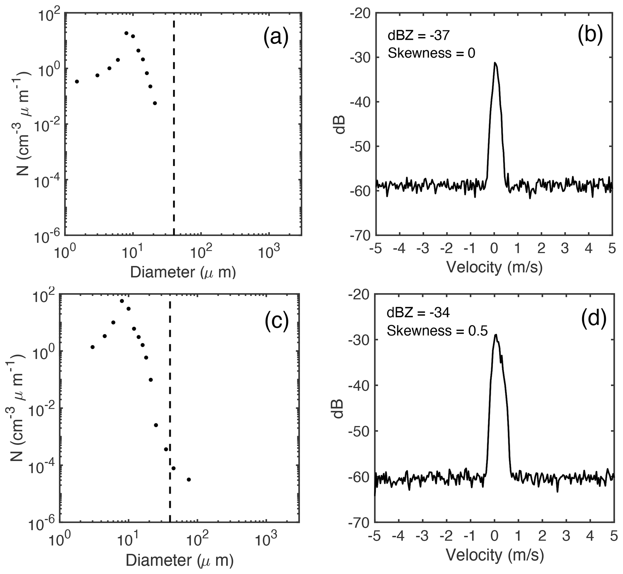
Figure 1 In situ observed DSD of cloud-only conditions (a) and the corresponding simulated Doppler radar spectrum (b); the reflectivity and skewness of the spectrum are indicated in the upper left corner. Panels (c) and (d) are the same as panels (a) and (b) but for mixed cloud-drizzle DSD. The dashed lines in panels (a) and (c) indicate a diameter of 40 µm.

Figure 1b and d show examples of the simulated Doppler spectra along with the estimated reflectivity and skewness for cloud-only and mixed cloud-drizzle DSDs. It is noticed for the drizzle case (Fig. 1d) that reflectivity is well below the conventional threshold (−20 to −15 dBZ) used for drizzle detection, so it cannot be discriminated from the cloud-only case (Fig. 1b). Skewness, however, shows a significant difference between drizzle (0.5) and cloud (0), emphasizing the importance of including skewness as an additional indicator for drizzle detection.

3.2 Machine learning algorithm application

From the IOP1 of ACE-ENA, 6000 in-situ-observed DSDs (2000 for cloud-only and 4000 for mixed cloud-drizzle conditions) are selected from the cloudy samples, defined as having liquid water contents larger than 0.01 g m⁻³ (Zhang et al., 2021). For each DSD, the spectrum simulator is applied to estimate the reflectivity and Doppler skewness. The distributions of these two quantities for all the selected datasets are shown in Fig. 2. This shows that drizzle with positive skewness tends to be associated with reflectivities lower than −20 dBZ. For reflectivities ranging from −35 to −25 dBZ and a skewness of around zero, the drizzle signal overlaps with that of cloud; this region represents the early stage of drizzle initiation, with low reflectivity and indistinguishable skewness features compared with cloud signals.

Figure 2 Distribution of the cloud-only (red points) and mixed cloud-drizzle (blue points) samples from in situ observations over the reflectivity–skewness space. The black line indicates the classification boundary of cloud/drizzle resolved by the machine learning algorithm. The right axis indicates the CDF of all correctly identified drizzly samples as a function of reflectivity obtained by each method: the dotted magenta line is for the in situ observations and represents the true value; the solid magenta line is for the ML technique; the magenta shading is for the reflectivity-based technique with an upper boundary of dBZ $>-\mathrm{20}$ and a lower boundary of dBZ $>-\mathrm{15}$; the dashed magenta line is for the reflectivity-threshold technique with dBZ $>-\mathrm{17}$.

In order to determine the classification boundary to distinguish cloud/drizzle categories (i.e., red/blue points in Fig. 2), we apply a supervised machine learning algorithm that is widely used in classification-related problems, the support vector machine (SVM) (Cortes and Vapnik, 1995; Vapnik et al., 1997). SVM handles complicated data classification tasks by solving optimization relationships and finding the optimal classification equations in the feature space. There are three reasons to use SVM in this study: (1) SVM is nonparametric and thus does not require the specification or assumption of the classification equation; (2) by applying the appropriate kernel, SVM can generate a nonlinear classification boundary to classify nonlinearly separable datasets; and (3) the decision boundary resolved by SVM will separate the categories with the maximum distance (this is a distinctive feature of the SVM algorithm which is extensively used in a variety of areas; Ma and Guo, 2014).

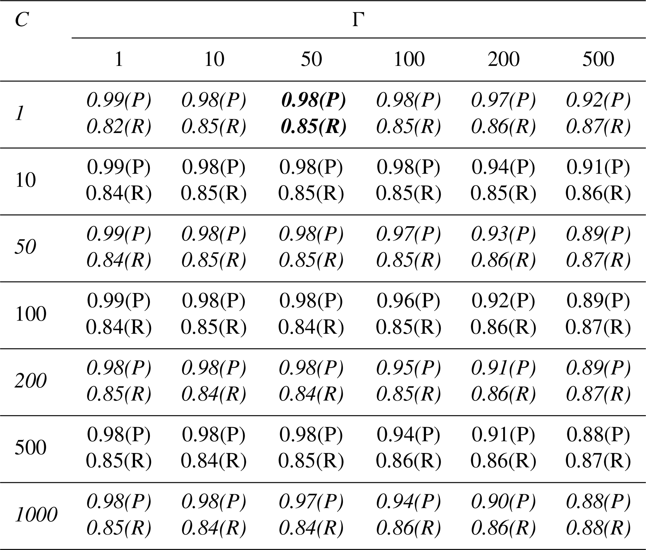
Of the collected cloud/drizzle datasets, 80 % are used for training and the remaining 20 % are used for validation. The inputs to the SVM are the Doppler skewness and reflectivity, where the reflectivity from −50 to 0 dBZ is normalized from −1 to 0; the output is classified as either cloud (0) or drizzle (1). Here, the radial basis function (RBF) with two tuning parameters, Γ and C, is used as the SVM kernel (Keerthi and Lin, 2003). The RBF kernel is one of the most widely used kernels due to its similarity to the Gaussian distribution. The Γ parameter determines the curvature of the decision boundary, with a high value indicating more curvature for capturing the complexity of the dataset. C is a regularization parameter to set the classification accuracy versus the maximization of the decision function margin; a lower C leads to a larger margin and a simpler decision function at the cost of training accuracy. Following Davis and Goadrich (2006), we use precision/recall to evaluate the performance of the classification outcome. In this study, “precision” refers to the number of correct drizzle detections divided by the total number of drizzle detections reported by the SVM, and “recall” refers to the number of correct drizzle detections divided by the number of true drizzle occurrences in the dataset. Different combinations of RBF parameters with Γ ranging from 1 to 500 and C from 1 to 1000 are applied, and the classification outcomes are shown in Table 1. Besides using the metrics recall and precision, the shape of the resolved boundary is also examined visually to avoid the ML algorithm being overfitted. As shown in Figs. S3–S8 in the Supplement, parameter with large C and Γ leads to a better classification outcome but will cause overfitting issues. Here we choose Γ=50 and C=1 as the preferred parameters to produce classification results with a precision and recall of 98 % and 85 %, respectively. That is, for the cloud-drizzle dataset collected during ACE-ENA, at most 85 % of the drizzle can be detected by the algorithm and, among the detection outcomes, 98 % are true drizzle signals.

Table 1 Precision (P) and recall (R) of the drizzle/cloud classification outcomes for different combinations of C and Γ. The values shown in bold italics represent the classification performance obtained for the parameters used in this study.

The resolved classification boundary is shown as a black line in Fig. 2. We can see that the algorithm separates the cloud/drizzle clusters reasonably well; the resolved skewness threshold that is used to distinguish cloud/drizzle is around ±0.2, and the maximum reflectivity used for classification is −20 dBZ. These values are consistent with previous studies (Frisch et al., 1995; Liu et al., 2008; Kollias et al., 2011b; Acquistapace et al., 2019). We further estimate the cumulative distribution function (CDF) of the correctly detected drizzle samples as a function of dBZ from the ML technique (solid magenta line in Fig. 2) and from the traditional method with the reflectivity threshold ranging from −20 to −15 dBZ (magenta shading in Fig. 2). It is noticeable that drizzle can be detected with dBZ $<-\mathrm{30}$ using the ML method; this value is significantly lower than for the traditional thresholds in use. The ML method is more sensitive to the weak drizzle signals than the dBZ thresholds that have been proposed. Specifically, compared to the ML technique, 35 % and 21 % of the drizzle are missed by the reflectivity threshold approach when using dBZ $>-\mathrm{20}$ and dBZ $>-\mathrm{15}$, respectively. Another important implication of this result is that dBZ $>-\mathrm{15}$ is traditionally applied by CloudSat to identify light rain incidence (Haynes et al., 2009); here, we demonstrate that a more robust threshold is likely to be much lower. More detailed performance comparisons of the two drizzle detection methods are shown in Fig. S9 in the Supplement, where the results are similar to those in Fig. 2; the rise of the false detection rate for the ML-based method for reflectivities lower than −20 dBZ is due to the existence of extremely weak drizzle signals, as will be discussed later.

Besides the encouraging performance of the ML technique, some noticeable issues can be identified. (1) Compared with the true CDF of the drizzle fraction (dotted magenta line in Fig. 2), 20 % of the drizzle is undetected. This missing drizzle subset, as explained previously by the overlapping area, is composed of tiny drizzle embryos that have yet to develop distinctive features compared with their cloud counterparts. (2) Another issue is the unrealistic broadening of the classification boundary for reflectivities lower than −35 dBZ; this issue is related to the kernel applied in the SVM algorithm. Since drizzle rarely exists below −35 dBZ, this issue will not affect the classification performance as far as we are concerned.

4 Results

The ML-based drizzle detection algorithm is applied to the dataset collected at three ARM observatories. First, an example case is presented for which aircraft observations are available and the corresponding in situ measurements are used to demonstrate the performance of the algorithm. Then, the drizzle occurrence for classified stratocumulus clouds at the ENA, MARCUS and MAGIC observatories are presented; the differences in drizzle occurrence from the proposed machine-learning-based algorithm (hereafter MLA) and the traditional dBZ-based algorithm (hereafter dBZA) are compared to show that drizzle occurrence in stratocumulus clouds is far more frequent than has been previously suggested. For the dBZA, we use reflectivity $>-\mathrm{17}$ dBZ for drizzle identification, while the application of other thresholds ranging from −20 to −15 dBZ did not affect the results as discussed.

4.1 Single cloud layer case

For the selected case (Fig. 3), a thin cloud layer with a thickness of around 150 m is identified. Cloud signals are very weak, with 99 % of the reflectivity being lower than −17 dBZ. However, the considerably large skewness values shown in Fig. 3b indicate the presence of drizzle particles. The classification results from the MLA classification are shown in Fig. 3c. It can be seen that drizzle is omnipresent and spread throughout the cloud layer, and is mixed with cloud-only detections.

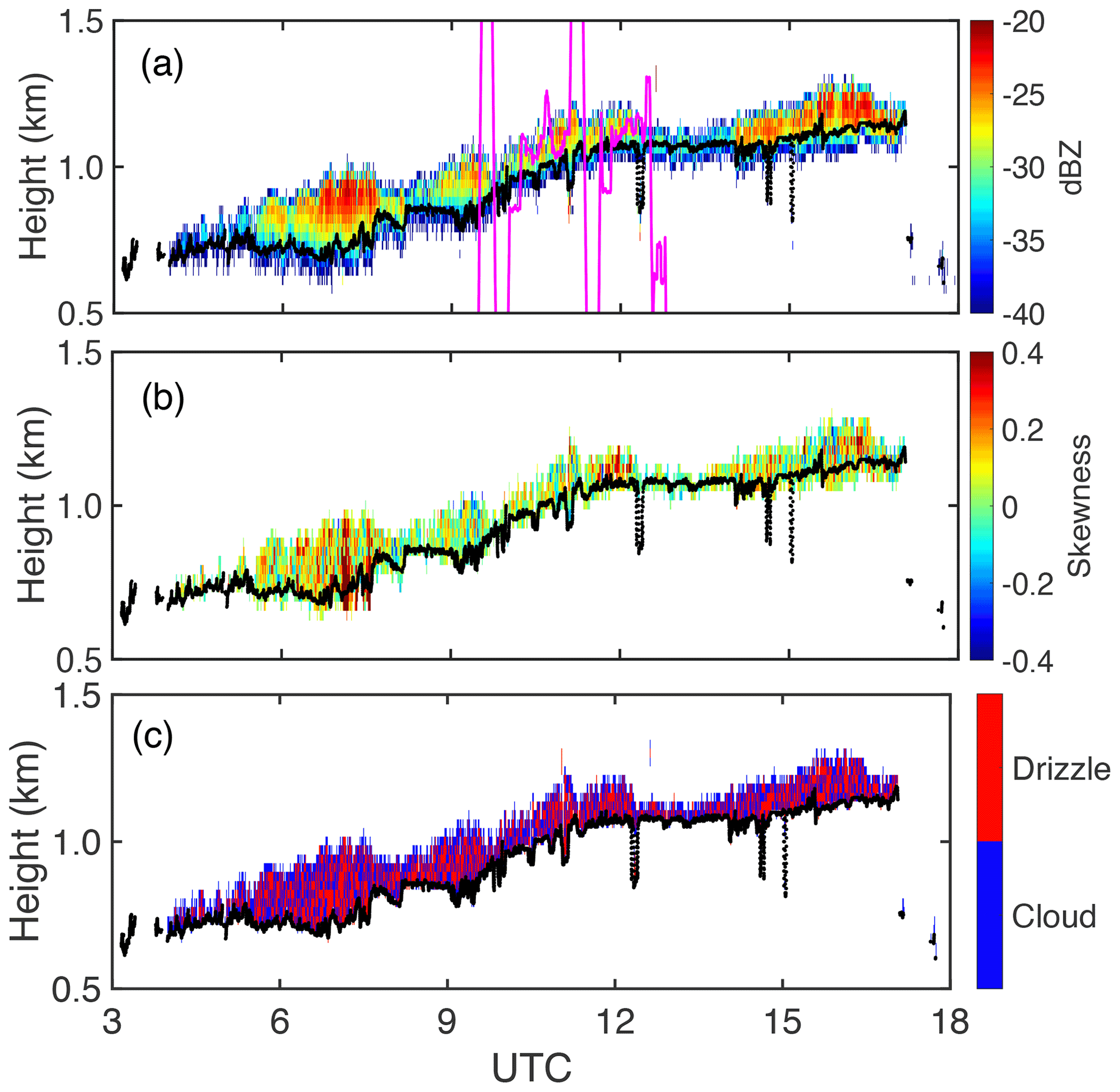
Figure 3 Reflectivity (a), skewness (b) and the classification mask (c) on 30 June 2017 at the ENA site. Black line indicates the ceilometer-determined cloud base; magenta line in (a) indicates the altitude track of the aircraft during the observation period.

Here, the in-situ-observed DSD is used to verify the MLA detection. On 30 June 2017, aircraft measurements were conducted from 09:27 to 13:16 UTC. We constrained the in situ measurements to be within 20 km of the ENA observatory (Fig. 4). Considering that the average in-cloud wind speed is 3.7 m s⁻¹, the distance of 20 km is equivalent to around 1.5 h of KAZR observations; thus, the radar measurements from 08:00 to 13:30 UTC are selected to match the aircraft observations. We assume that the signal for drizzle/cloud occurrence collected from the in situ measurements can be used to verify the drizzle presence observed from KAZR. For the selected period, drizzle occurrence is 47 % from the MLA detections and 65 % from the in-situ observations. The 18 % of the drizzle missed by MLA is largely attributed to the overlapping area shown in Fig. 2; this area indicates early-stage drizzle embryos that are indistinguishable from cloud droplets. Nevertheless, this comparison provides strong evidence that drizzle is widely present in the cloud layer for the selected case and demonstrates that the classification results from MLA are reliable. Contrastingly, negligible drizzle signals (0.05 %) are detected with the reflectivity-based (dBZ $>-\mathrm{17}$) technique.

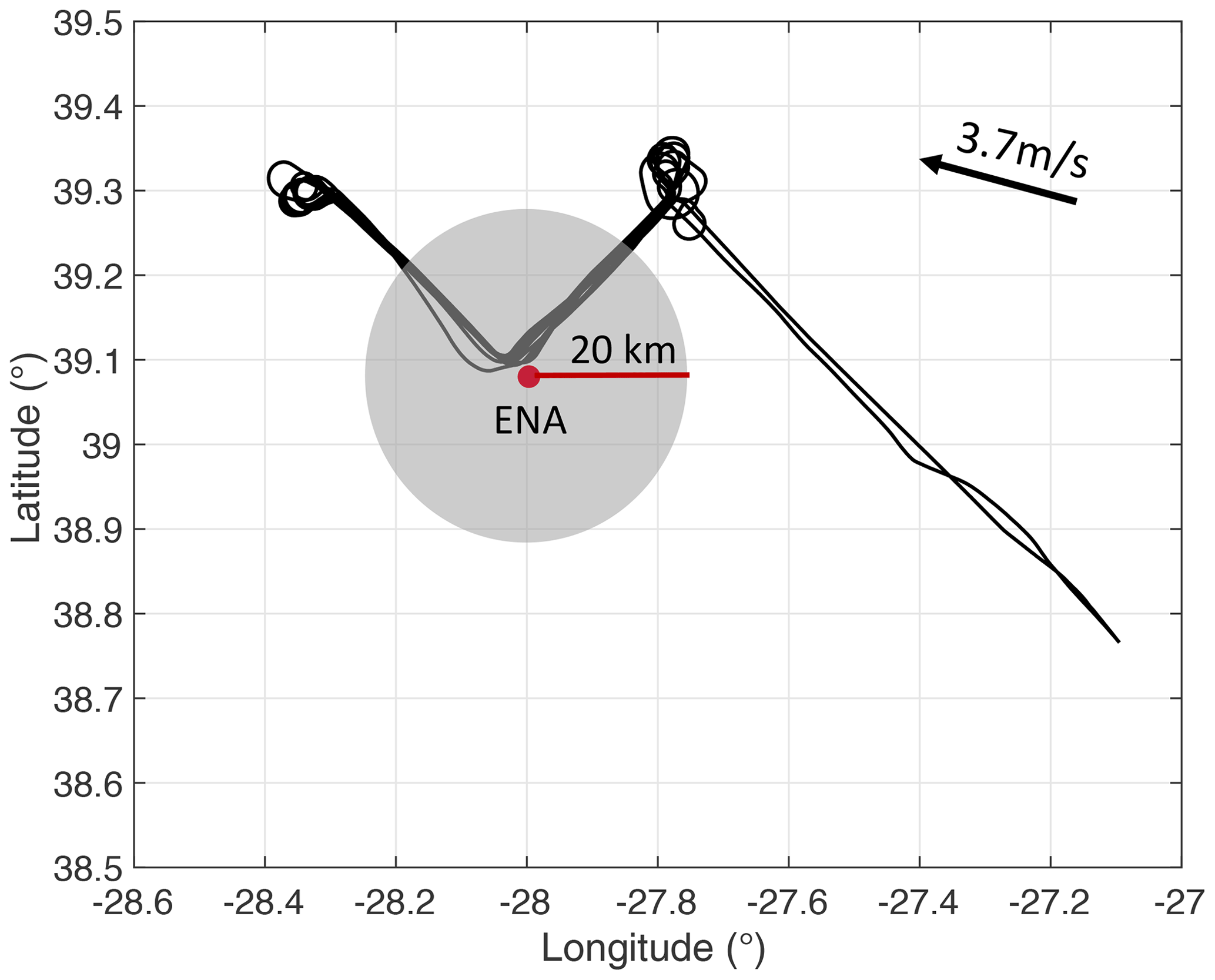
Figure 4 Aircraft track (black line) during the operational period on 30 June 2017. Shaded circle indicates the area within 20 km around the ENA site. The arrow in the upper right corner indicates the mean wind direction and wind velocity in the cloud layer during the observational period.

4.2 Drizzle occurrence at ARM campaigns

During the operational periods of ACE-ENA, MARCUS and MAGIC, single-layer marine stratocumulus clouds with cloud top temperatures greater than 0 ^∘C and cloud top heights lower than 4000 m are selected. The moving standard deviation of cloud top height within 30 min (σ) is calculated and profiles with σ larger than 200 m are excluded to reject non-stratocumulus-type clouds. LWP retrievals are biased when MWR is wet; thus, radar profiles for which the lowest range gates contain hydrometeor detections are considered to be precipitation and are removed from the analysis. A complete list of the days used is shown in Table 2. In total, 204, 72 and 215 h of radar observation were selected from the ACE-ENA, MARCUS and MAGIC campaigns.

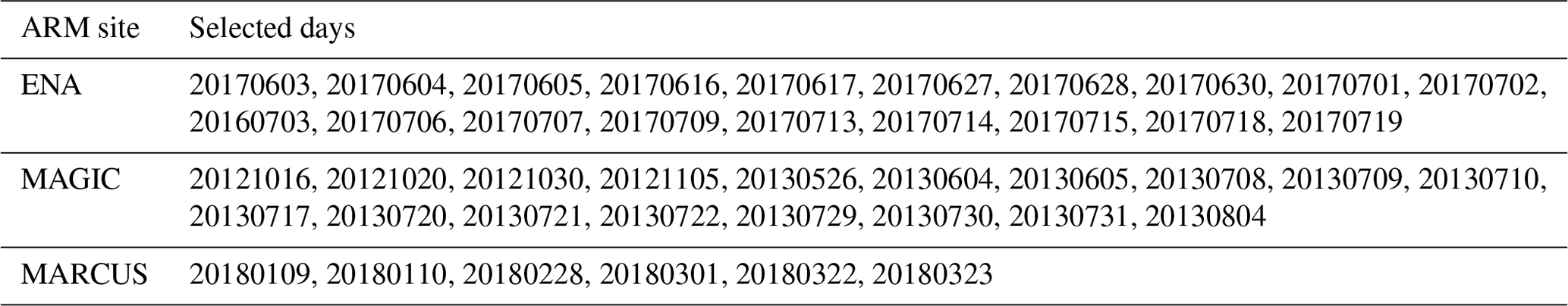
Table 2 Selected stratocumulus days in the ACE-ENA, MAGIC and MARCUS campaigns.

In order to composite cloud layers with different thicknesses, cloud height is normalized between 0 to 1 as

$$h={\displaystyle \frac{H-H_{\mathrm{b}}}{H_{\mathrm{t}}-H_{\mathrm{b}}}},$$

where H is the physical height of a given radar gate, and H_t and H_b are the cloud top and base heights, respectively. h=0 represents the cloud base and h=1 indicates the cloud top.

Drizzle occurrence is calculated as the number of drizzle detections divided by the total number of observed signals in each normalized height bin (0.1) and LWP bin (50 g m⁻²). The drizzle occurrences detected from both methods at the three ARM observatories are shown in Fig. 5. For all the observational sites/campaigns, drizzle is more likely to occur as LWP increases. This tendency holds true regardless of the drizzle detection method being used. However, for each observational campaign, the drizzle occurrence detected from MLA (Fig. 5a, b, c) is always larger than that from dBZA (Fig. 5d, e, f). This difference becomes especially significant for thin clouds with low LWP: when the LWP is under 50 g m⁻² or, equivalently, the cloud thickness is less than 200 m (Fig. 6), the drizzle occurrence detected from dBZA is around 0.1, while it is 0.4–0.5 from MLA. This result clearly indicates that the traditional drizzle detection method based on a reflectivity threshold significantly underestimates the true drizzle occurrence, especially in thin cloud layers. To quantitatively describe the detection performance, we estimate the relative percentage difference in drizzle detections between the two methods as follows:

$$P_{\mathrm{LWP}}\left(\mathit{\%}\right)={\displaystyle \frac{N_{\mathrm{MLA},\mathrm{LWP}}-N_{\mathrm{dBZA},\mathrm{LWP}}}{N_{\mathrm{MLA},\mathrm{LWP}}}}\times \mathrm{100},$$

where N_MLA, LWP and N_dBZA, LWP indicate the number of drizzle detections by MLA and dBZA, respectively, for a given LWP category. The results (Fig. 7a) indicate that when LWP is smaller than 50 g m⁻², which frequently occurs in the ENA and MAGIC campaigns (Fig. 7b), 90 % of the drizzle is missed by dBZA at ENA and MARCUS, and 60 % of the drizzle is undetected at MAGIC compared with MLA. The application of a relatively low reflectivity threshold with dBZ $<-\mathrm{20}$ mitigates the missing drizzle detections compared with MBL to some degree, but 50 %–80 % of the drizzle is still undetected (shaded area in Fig. 7a).

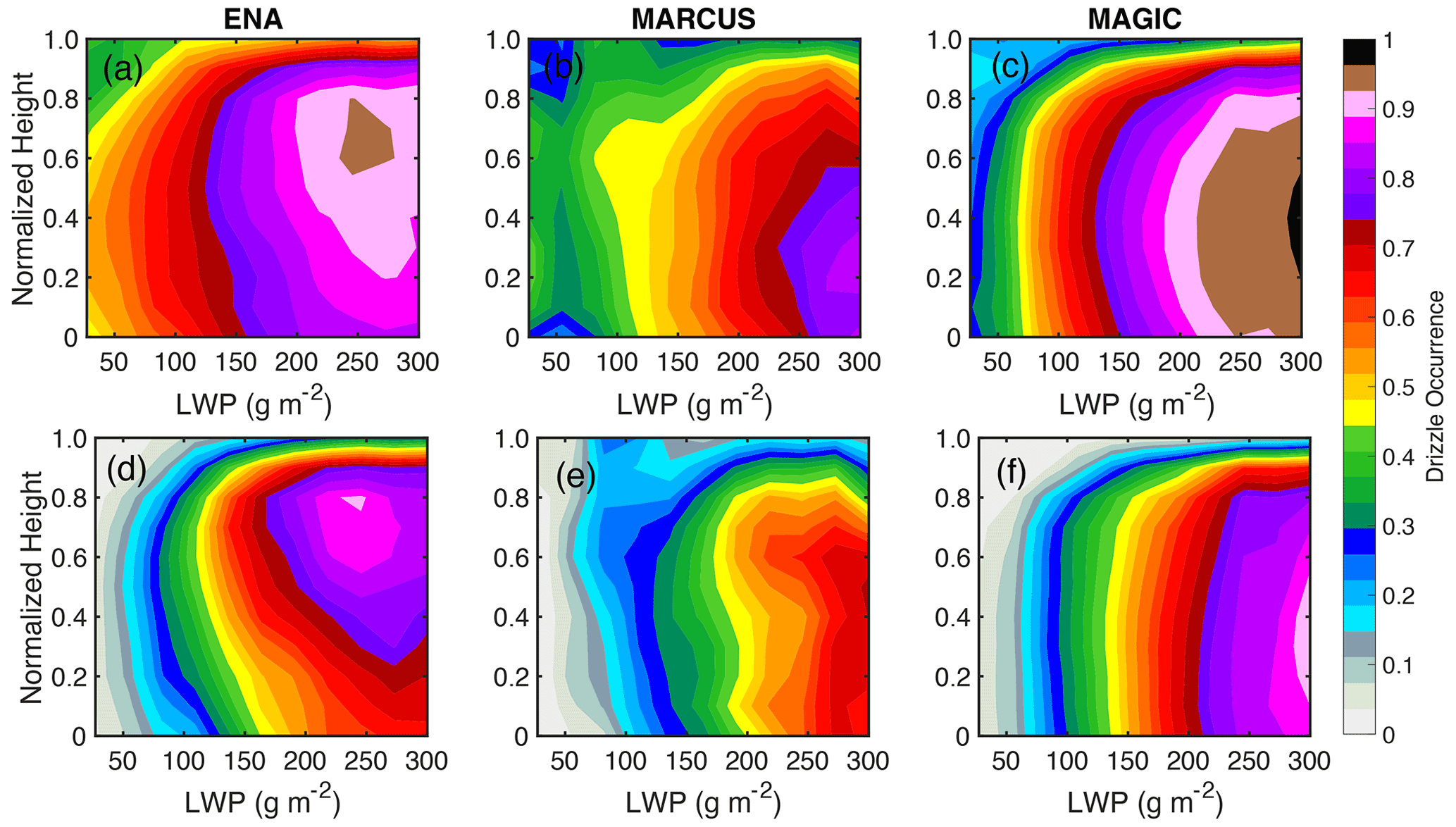
Figure 5 Vertical distribution of drizzle occurrence categorized by LWP based on MLA in the ENA (a), MARCUS (b) and MAGIC (c) observational campaigns. Panels (d), (e) and (f) are the same as panels (a), (b) and (c) except that the drizzle is detected by dBZA.

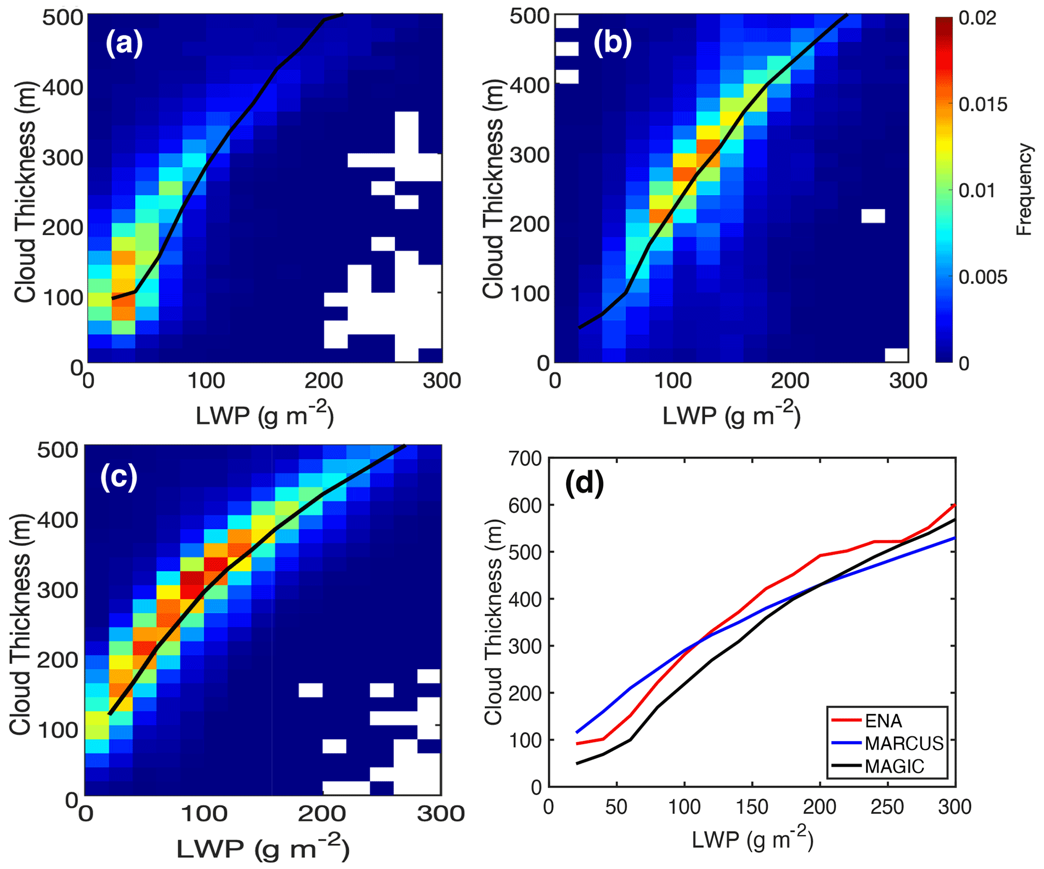
Figure 6 Joint histograms of cloud thickness and LWP in three campaigns: (a) ENA, (b) MARCUS and (c) MAGIC. The black line indicates the mean cloud thickness in each LWP category. For comparison, the relationships between mean cloud thickness and LWP in the three campaigns (black lines in a, b and c) are shown in (d).

Figure 7 (a) Relative percentage difference in drizzle detection between the dBZA (dBZ $>-\mathrm{17}$) and MLA as a function of LWP in ARM observational campaigns: ENA (red line), MARCUS (blue line) and MAGIC (black line). The shaded area indicates the same results but with a different reflectivity threshold: the upper boundary is for dBZ $>-\mathrm{15}$ and the lower boundary is for dBZ $>-\mathrm{20}$. (b) Histograms of the LWP distribution collected in three campaigns: ENA (red line), MARCUS (blue line) and MAGIC (black line).

Besides the considerable drizzle signals missed by dBZA, another implication to be noted is the differences in drizzle distribution among the three ARM campaigns. Specifically, large drizzle fractions tend to occur in the upper part of the cloud at ENA and in the lower part of the cloud at MARCUS and MAGIC (Fig. 5). When compared with MLA, the missing drizzle detections based on dBZA are much more significant for ENA/MARCUS than for MAGIC (Fig. 7a). The different drizzle distribution patterns suggest that the clouds studied in the three campaigns may differ in the microphysical properties and processes that control drizzle initiation. For instance, the contrasting thermodynamic environments in the ARM campaigns, with low/high temperature and humidity at MARCUS/MAGIC, might lead to different autoconversion processes that control the drizzle formation. In particular, we suspect that a more humid environment at MAGIC will benefit the generation of larger cloud droplets compared with the other campaigns (Laird et al., 2000; Zhou et al., 2015). Figure 8 supports this hypothesis by showing that the mean cloud reflectivity at MAGIC is 8 dB larger than it is in the other two campaigns for LWPs smaller than 100 g m⁻². The relatively large dBZ for small LWPs mitigates the underrepresented drizzle detection by the reflectivity-based method to some degree.

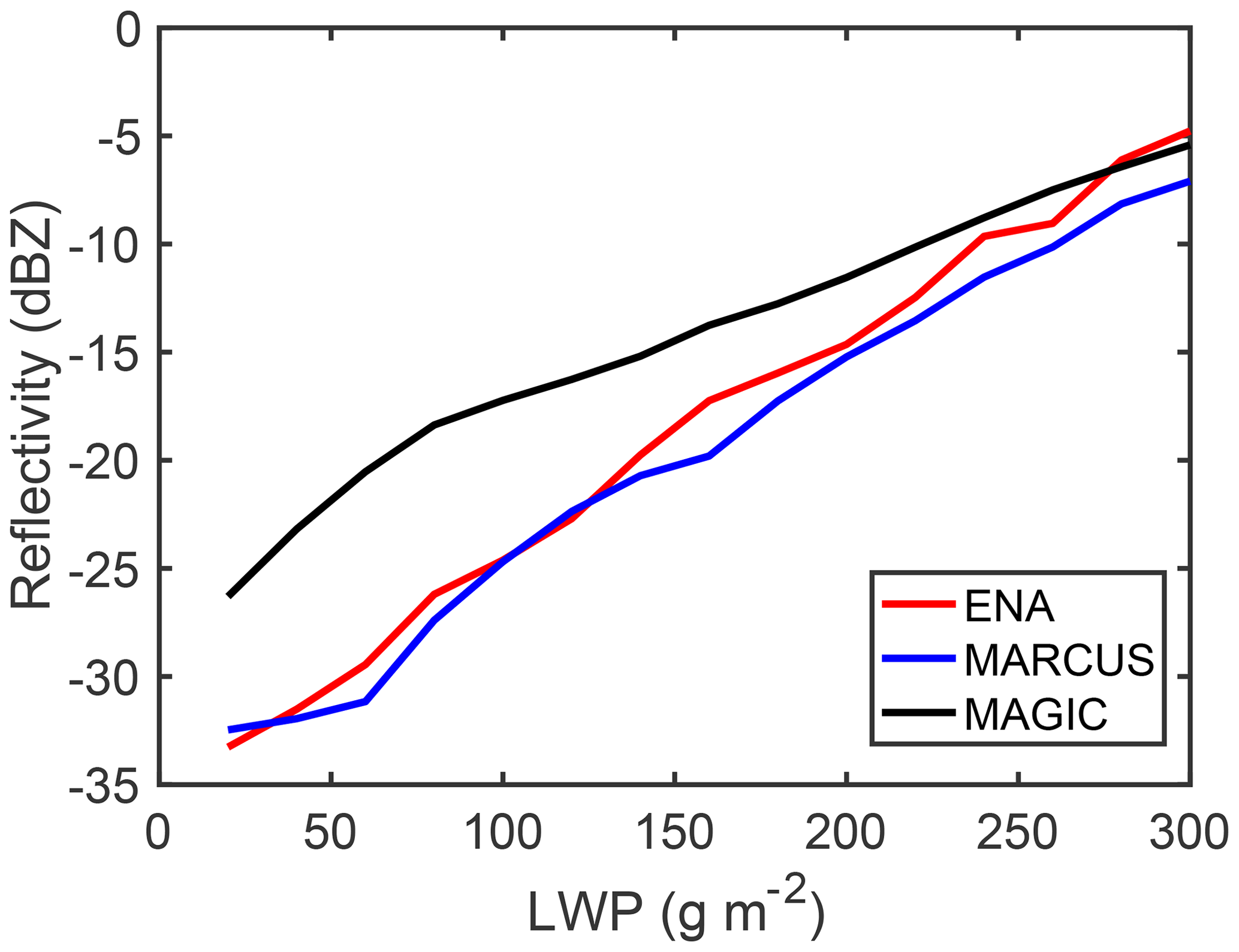
Figure 8 Mean KAZR reflectivity of the hydrometeor signal as a function of LWP in three campaigns: ENA (red line), MARCUS (blue line) and MAGIC (black line).

5 Conclusion and discussion

Building on the concept that radar Doppler spectra skewness is more sensitive to drizzle presence, a new method of detecting drizzle in marine boundary clouds has been presented. In-situ-observed DSDs were used to unambiguously classify cloud and drizzle particles; then, a radar Doppler spectra simulator was applied to estimate the expected radar-observed reflectivity and skewness. Extensive datasets collected from the ACE-ENA campaign were trained via the ML-based algorithm to optimally determine a classification equation for cloud/drizzle. The proposed algorithm was validated by the in situ measurements as being able to successfully detect weak drizzle signals, which are completely missed by the traditional reflectivity-based technique.

The drizzle/cloud classification outcome for a thin cloud layer observed on 30 June 2017 at ENA was presented to show the performance of the detection algorithm. It was found that even for thin cloud with a thickness of less than 150 m, a significant amount of drizzle already exists; this classification result was further verified by the in situ observations. Furthermore, a statistical analysis compared the drizzle occurrences in the ACE-ENA, MARCUS and MAGIC field campaigns from two detection methods. The results indicated that drizzle is ubiquitous in cloud layers and its existence has been significantly underestimated by conventional reflectivity-based methods, especially in thin cloud layers. The ubiquity of drizzle in the MBL clouds calls for investigations on the drizzle formation mechanism. It is known that the growth of liquid droplets by diffusion is not efficient for a radius larger than 20 µm; thus, other mechanisms that favor drizzle formation greatly contribute to the existence of drizzle. The presented results provide observational evidence to verify the drizzle formation theories. The drizzle occurrence and vertical structure differ among the three campaigns, indicating that drizzle formation and distribution in marine stratocumulus clouds might be regime dependent, i.e., determined by microphysical and dynamical processes in the local region. In this study, data from the three observational campaigns are used to explore the drizzle frequency of marine stratocumulus in middle/high-latitude regions; however, it is quite possible that the drizzle occurrence in other locations might differ from the presented results. A complete understanding of the drizzle climatology in marine stratocumulus clouds calls for more campaign observations and continuing investigations.

The results in this study provide a new perspective for viewing drizzle existence in radar observations in the hope of shedding light on several critical topics in warm cloud studies. (1) In most microphysics retrieval algorithms, the existence of drizzle particles is determined by a reflectivity threshold. However, this study shows the presence of significant drizzle drops during low-reflectivity conditions (lower than −20 dBZ), and a lack of consideration of these drops may lead to a certain degree of retrieval uncertainty. (2) Drizzle production mechanisms are widely regarded as a critical missing piece of the puzzle in warm cloud research (Takahashi et al., 2017). In particular, there are large variations among the parameterization schemes of the autoconversion/accretion processes used in numerical models, leading to significant uncertainty in future climate predictions (Michibata and Suzuki, 2020; Wood, 2005b). The results presented in this study can be used to verify the proposed parameterization schemes by comparing the drizzle climatology. (3) Furthermore, the novel utilization of the synthesis of in situ and remote sensing observations presented in this study yields insights on the potential of combined multi-platform observations to investigate the microphysical processes in warm clouds.