the Creative Commons Attribution 4.0 License.
the Creative Commons Attribution 4.0 License.
 | 09 May 2022
Iron from coal combustion particles dissolves much faster than mineral dust under simulated atmospheric acidic conditions
Clarissa Baldo
Michael D. Krom
Weijun Li
Tim Jones
Nick Drake
Konstantin Ignatyev
Nicholas Davidson
Mineral dust is the largest source of aerosol iron (Fe) to the offshore global ocean, but acidic processing of coal fly ash (CFA) in the atmosphere could be an important source of soluble aerosol Fe. Here, we determined the Fe speciation and dissolution kinetics of CFA from Aberthaw (United Kingdom), Krakow (Poland), and Shandong (China) in solutions which simulate atmospheric acidic processing. In CFA PM10 fractions, 8 %–21.5 % of the total Fe was found to be hematite and goethite (dithionite-extracted Fe), and 2 %–6.5 % was found to be amorphous Fe (ascorbate-extracted Fe), while magnetite (oxalate-extracted Fe) varied from 3 %–22 %. The remaining 50 %–87 % of Fe was associated with other Fe-bearing phases, possibly aluminosilicates. High concentrations of ammonium sulfate ((NH4)2SO4), often found in wet aerosols, increased Fe solubility of CFA up to 7 times at low pH (2–3). The oxalate effect on the Fe dissolution rates at pH 2 varied considerably, depending on the samples, from no impact for Shandong ash to doubled dissolution for Krakow ash. However, this enhancement was suppressed in the presence of high concentrations of (NH4)2SO4. Dissolution of highly reactive (amorphous) Fe was insufficient to explain the high Fe solubility at low pH in CFA, and the modelled dissolution kinetics suggest that other Fe-bearing phases such as magnetite may also dissolve relatively rapidly under acidic conditions. Overall, Fe in CFA dissolved up to 7 times faster than in a Saharan dust precursor sample at pH 2. Based on these laboratory data, we developed a new scheme for the proton- and oxalate-promoted Fe dissolution of CFA, which was implemented into the global atmospheric chemical transport model IMPACT (Integrated Massively Parallel Atmospheric Chemical Transport). The revised model showed a better agreement with observations of Fe solubility in aerosol particles over the Bay of Bengal, due to the initial rapid release of Fe and the suppression of the oxalate-promoted dissolution at low pH. The improved model enabled us to predict sensitivity to a more dynamic range of pH changes, particularly between anthropogenic combustion and biomass burning aerosols.
- Article
(8612 KB) - Full-text XML
-
Supplement
(983 KB) - BibTeX
- EndNote


The availability of iron (Fe) limits primary productivity in high-nutrient, low-chlorophyll (HNLC) regions of the global ocean, including the subarctic North Pacific, the eastern Equatorial Pacific, and the Southern Ocean (Boyd et al., 2007; Martin, 1990). In other regions of the global ocean, such as the subtropical North Atlantic, the Fe input may affect primary productivity by stimulating nitrogen fixation (Mills et al., 2004; Moore et al., 2006). These areas are particularly sensitive to changes in the supply of bioavailable Fe. Atmospheric aerosols are an important source of soluble (and, thus, potentially bio-accessible) Fe to the offshore global ocean. The deposition of bio-accessible Fe to the ocean can alter biogeochemical cycles and increase the carbon uptake, consequently affecting the climate (e.g. Jickells and Moore, 2015; Jickells et al., 2005; Kanakidou et al., 2018; Mahowald et al., 2010; Shi et al., 2012). In general, bio-accessible Fe consists of aerosol-dissolved Fe, and Fe nanoparticles which can be present in the original particulate matter and/or formed during atmospheric transport as a result of cycling into and out of clouds (Shi et al., 2009). It is, in addition, possible that other more refractory forms of Fe could be solubilized in the surface waters by zooplankton (Schlosser et al., 2018) or the microbial community (Rubin et al., 2011).
The Fe transported in the atmosphere is largely derived from lithogenic sources, which contribute around 95 % of the total Fe in suspended particles (e.g. Shelley et al., 2018), and most studies so far have concentrated on the atmospheric processing of mineral dust (e.g. Cwiertny et al., 2008; Fu et al., 2010; Ito and Shi, 2016; Shi et al., 2011a, 2015). Mineral dust has low Fe solubility (dissolved Fe total Fe × 100) near the source regions, generally below 1 % (e.g. Shi et al., 2011; Sholkovitz et al., 2009, 2012), increasing somewhat as a result of processes occurring during atmospheric transport (e.g. Baker et al., 2021, 2020). Other sources of bio-accessible Fe to the ocean are from combustion sources such as biomass burning, coal combustion, oil combustion, and metal smelting (e.g. Ito et al., 2018; Rathod et al., 2020). Although these sources are only a small fraction of the total Fe in atmospheric particulates, the Fe solubility of pyrogenic sources can be 1–2 orders of magnitude higher than in mineral dust (Ito et al., 2021b and references therein) and, thus, can be important in promoting carbon uptake. However, the Fe solubility of pyrogenic sources varies considerably, depending on the particular sources, with higher values observed for oil combustion and biomass burning than coal combustion sources (Ito et al., 2021b and references therein).
Wang et al. (2015) estimated that coal combustion emitted around ∼ 0.9 Tg yr−1 of Fe into the atmosphere (on average for 1960–2007), contributing up to ∼ 86 % of the total anthropogenic Fe emissions. A more recent study, which has included metal smelting as an atmospheric Fe source, estimated that coal combustion emitted ∼ 0.7 Tg yr−1 of Fe for the year 2010, contributing around 34 % of the total anthropogenic Fe atmospheric loading (Rathod et al., 2020). Although the use of coal as a principal energy source has been recently reduced as a result of concerns about air quality and global warming, coal is still an important energy source in a number of countries, in particular in the Asia–Pacific region (BP, 2020). In China, most of the total energy is supplied by coal, contributing over 50 % of the global coal consumption in 2019, followed by India (12 %), and the USA (8 %). Germany and Poland are the largest coal consumers in Europe, accounting together for around 40 % of the European usage (BP, 2020). South Africa is also among the principal countries for coal consumption (BP, 2020) and is a source of Fe-bearing particles to the anaemic Southern Ocean (e.g. Ito et al., 2019).
Coal fly ash (CFA) is a by-product of coal combustion. This generally consists of glassy spherical particles (e.g. Brown et al., 2011) which are formed through different transformations (decomposition, fusion, agglomeration, and volatilization) of mineral matter in coal during combustion (e.g. Jones, 1995) and are transported with the flue gases undergoing rapid solidification. CFA is co-emitted with acidic gases such as sulfur dioxide (SO2), nitrogen oxides (NOx), and carbon dioxide (CO2; e.g. Munawer, 2018).
During long-range transport, CFA particles undergo atmospheric processing with the CFA surface coated by acidic species, such as sulfuric acid (H2SO4) and oxalic acid (H2C2O4), in atmospheric aerosols. Aged CFA particles are hygroscopic and absorb water at typical relative humidity in the marine atmosphere. As a result, a thin layer of water with high acidity, low pH, and high ionic strength is formed around the particles (Meskhidze et al., 2003; Spokes and Jickells, 1995; Zhu et al., 1992). In addition, ammonia (NH3), which is a highly hydrophilic gas, can also partition into the aerosol phase, react with H2SO4, and form ammonium sulfate ((NH4)2SO4), which is an important inorganic salt contributing to the high ionic strength in aged atmospheric aerosols (Seinfeld and Pandis, 2016).
At low pH conditions, Fe solubility in aerosols increases, as the high concentration of protons (H+) weakens the Fe–O bonds facilitating the detachment of Fe from the surface lattice (Furrer and Stumm, 1986). Li et al. (2017) provided the first observational evidence that acidification leads to the release of Fe from anthropogenic particles.
In addition to these inorganic processes, organic ligands can also enhance atmospheric Fe dissolution by forming soluble complexes with Fe (e.g. Cornell and Schwertmann, 2003). For example, H2C2O4 is an important organic species in aerosols (e.g. Kawamura and Bikkina, 2016). Laboratory studies have demonstrated that H2C2O4 increases Fe solubility of aerosol sources (Chen and Grassian, 2013; Johnson and Meskhidze, 2013; Paris and Desboeufs, 2013; Paris et al., 2011; Xu and Gao, 2008). Recently, observations over the Bay of Bengal indicate that H2C2O4 contributes to the increase in dissolved Fe in atmospheric water (Bikkina et al., 2020).
To simulate the Fe dissolution in CFA, it is necessary to determine the dissolution kinetics under realistic conditions. Previous studies have investigated the Fe dissolution kinetics of CFA under acidic conditions. Chen et al. (2012) simulated acidic and cloud processing of certified CFA. Fu et al. (2012) determined the dissolution kinetics of CFA samples at pH 2, while Chen and Grassian (2013) investigated the effect of organic species (e.g. oxalate and acetate) at pH 2–3. These studies showed that high acidity and the presence of oxalate enhanced Fe dissolution at the surface of CFA particles, similar to those reported in mineral dust (Chen et al., 2012; Chen and Grassian, 2013; Fu et al., 2012; Ito and Shi, 2016; Shi et al., 2011a). They also demonstrated that there are large differences in dissolution rates in different types of CFA, likely related to the Fe speciation.
Furthermore, high ionic strength, commonly seen in aerosol water, affects the activity of molecular species present in solution; consequently, it can significantly impact the Fe dissolution behaviour. Recent studies have considered the effect of the high ionic strength on the Fe dissolution kinetics of CFA under acidic conditions. For example, the Fe solubility of CFA samples was measured at pH 1–2 with high sodium chloride (NaCl) concentrations (Borgatta et al., 2016) and with high sodium nitrate (NaNO3) concentrations (Kim et al., 2020). In real atmospheric conditions, NaCl or NaNO3 are unlikely to be the main drivers of high ionic strength in aged CFA. Although NaCl can coagulate with dust particles in the marine boundary layer (Zhang et al., 2003), the ageing of CFA is primarily by the uptake of secondary species, particularly sulfate and ammonia (Li et al., 2003). Ito and Shi (2016) found that, at low pH and a high concentration of (NH4)2SO4, the Fe solubility of mineral dust is likely to be enhanced by the adsorption of sulfate ions on the particle surface. However, to date the effect of high (NH4)2SO4 concentrations on the Fe dissolution behaviour in combustion sources in the presence or absence of oxalate remains unknown.
The dissolution kinetics measured by Chen and Grassian (2013) have been used to develop a modelled dissolution scheme for CFA, assuming a single Fe-bearing phase in CFA (Ito, 2015). However, there are multiple Fe-bearing phases in CFA, primarily hematite, magnetite, and Fe in aluminium silicate glass (Brown et al., 2011; Chen et al., 2012; Fu et al., 2012; Kukier et al., 2003; Kutchko and Kim, 2006; Lawson et al., 2020; Sutto, 2018; Valeev et al., 2019; Waanders et al., 2003; Wang, 2014; Zhao et al., 2006), but there are also accessory Fe-bearing minerals, for example, silicates, carbonate, sulfides, and sulfates (Zhao et al., 2006). These phases have a range of reactivities. Previous studies showed that CFA dissolves much faster during the first 1–2 h than subsequently (Borgatta et al., 2016; Chen et al., 2012; Chen and Grassian, 2013; Fu et al., 2012; Kim et al., 2020), confirming the existence of multiple Fe-bearing phases within a single CFA sample with different dissolution behaviour.
In this study, laboratory experiments were conducted to determine the dissolution kinetics of coal combustion emission products (i.e. CFA) during simulated atmospheric acidic processing in the presence of (NH4)2SO4 and oxalate, which are commonly found in atmospheric aerosols. In particular, we investigated the effect of high (NH4)2SO4 concentrations on the proton-promoted and oxalate-promoted Fe dissolution at low pH conditions. Our study also determined the Fe-bearing phases present in the CFA and compared them to those present in mineral dust. The experimental results enabled us to develop a new Fe release scheme for CFA sources, which was then implemented into the global atmospheric chemical transport model IMPACT (Integrated Massively Parallel Atmospheric Chemical Transport). The model results were compared with observations of Fe solubility in aerosol particles over the Bay of Bengal from Bikkina et al. (2020).
2.1 Sample collection and subsequent size fractionation
CFA samples were collected from the electrostatic precipitators at three coal-fired power stations at different locations in the United Kingdom (Aberthaw ash), Poland (Krakow ash), and China (Shandong ash). The bulk samples were resuspended to obtain aerosol fractions representative of particles emitted into the atmosphere. A custom-made resuspension system was used to collect the PM10 fraction (particles with an aerodynamic diameter smaller than 10 µm), which is shown in Fig. S1 in the Supplement. Around 20 g of sample was placed into a glass bottle and injected at regular intervals (2–5 s) into a glass reactor (∼ 70 L) by flushing the bottle with pure nitrogen. The air in the reactor was pumped at a flow rate of 30 L min−1 into a PM10 sampling head. Particles were collected on 0.6 µm polycarbonate filters and transferred into centrifuge tubes. The system was cleaned manually and flushed for 10 min with pure nitrogen before loading a new sample. A soil sample from Libya (Soil 5; 32.29237∘ N, 22.30437∘ E) was dry sieved to 63 µm and used as an analogue for a Saharan mineral dust precursor to make a comparison between CFA and mineral dust.
2.2 Fe dissolution kinetics
The Fe dissolution kinetics of the CFA samples were determined by time-dependent leaching experiments. We followed a similar methodology as in Ito and Shi (2016). PM10 fractions were exposed to H2SO4 solutions at pH 1, 2, or 3 in the presence of H2C2O4 and/or (NH4)2SO4 to simulate acidic processing in aerosol conditions. The concentration of H2C2O4 in the experiment solutions was chosen based on the molar ratio of oxalate and sulfate in PM2.5 (particles with an aerodynamic diameter smaller than 2.5 µm) from observations over the East Asia region (Yu et al., 2005). Around 50 mg of CFA was leached in 50 mL of acidic solution to obtain a particles liquid ratio of 1 g L−1. The sample solution was mixed continuously in a rotary mixer, in the dark, at room temperature. A volume of 0.5 mL was sampled at fixed time intervals (2.5, 15, and 60 min and 2, 6, 24, 48, 72, and 168 h after the CFA sample was added to the experiment solution) and filtered through 0.2 µm pore size syringe filters. The dissolved Fe concentration in the filtrate was determined using the ferrozine method (Viollier et al., 2000). Leaching experiments were also conducted on the Libyan dust precursor sample. The relative standard deviation (RSD) at each sampling time varied from 4 % to 15 % (n=7).
The pH of all the experiment solutions was calculated using the E-AIM III model for aqueous solutions (Wexler and Clegg, 2002). This was partly because the high ionic strength generated by the elevated concentration of (NH4)2SO4 prevents electrochemical sensors from making accurate pH measurements. For the experiment solutions with no (NH4)2SO4, the pH was measured by a pH meter before adding the ash and at the end of the experiments. The solution pH increased after adding the ash, and the change in pH was used to estimate the buffer capacity of alkaline minerals in the samples, including for example calcium carbonates (CaCO3), lime (CaO), and portlandite (Ca(OH)2). The estimated concentration of the H+ buffered was used to input the concentration of H+ into the E-AIM model. For each experiment, the pH was calculated before adding the CFA samples and at the end of the experiments. The pH of the original solution before adding the samples was estimated from the molar concentrations (mol L−1) of H2SO4, H2C2O4, and (NH4)2SO4 used to prepare the solution. The model inputs included the total concentrations of H+ (without H2C2O4 contribution), NH, SO, and H2C2O4. For the experiment solutions with no (NH4)2SO4, we calculated the final pH by reducing the total H+ concentration input into the model to match the pH measured at the end of the experiments. The buffered H+ was then estimated from the difference between the original and final H+ concentration input into the model. To determine the final pH of the solutions with high ionic strength, the H+ concentration input in the model was calculated as the difference between the H+ concentration in the original solution and the buffered H+ estimated at low ionic strength.
For the solution with no (NH4)2SO4, the difference between calculated and measured pH is <7 %. Table S1 in the Supplement reports the concentrations of H2SO4, H2C2O4, and (NH4)2SO4 in the experiment solutions, the original and final pH from model estimates (including H+ concentrations and activities), and the pH measurements for the solution with low ionic strength.
2.3 Sequential extractions
The content of Fe oxide species in the samples was determined by Fe sequential extraction (Baldo et al., 2020; Poulton and Canfield, 2005; Raiswell et al., 2008; Shi et al., 2011b). The Fe oxide species included highly reactive amorphous Fe oxide–hydroxide (FeA), crystalline Fe oxide–hydroxide, mainly goethite and hematite (FeD), and Fe associated with magnetite (FeM).
To extract FeA, samples were leached in an ascorbate solution buffered at pH 7.5 (Raiswell et al., 2008; Shi et al., 2011b). The ascorbate solution contained a deoxygenated solution of 50 g L−1 sodium citrate, 50 g L−1 sodium bicarbonate, and 10 g L−1 of ascorbic acid. Around 30 mg of CFA was leached for 24 h in 10 mL of ascorbate extractant and mixed continuously in a rotary mixer. The extraction solution was then filtered through a 0.2 µm membrane filter. In order to extract FeD, the residue was leached for 2 more hours in a dithionite solution buffered at pH 4.8 (50 g L−1 sodium dithionite in 0.35 M acetic acid and 0.2 M sodium citrate; Raiswell et al., 2008; Shi et al., 2011b).
For the extraction of FeM, the CFA samples were first leached for 2 h, using a citrate-buffered dithionite solution which, not sequential to the ascorbate extraction, will remove FeD and FeA. The residue collected after filtration was then leached for 6 h in a solution of 0.2 M ammonium oxalate ((NH4)2C2O4) and 0.17 M H2C2O4 at pH 3.2 (Poulton and Canfield, 2005). The Fe extractions were all carried out in the dark at room temperature. The Fe concentration in the filtered extraction solutions was measured using the ferrozine method (Viollier et al., 2000) or by inductively coupled plasma optical emission spectrometry (ICP-OES) analysis for the solutions containing a high concentration of oxalate.
The total Fe content in the samples was determined by microwave digestion in concentrated nitric acid (HNO3), followed by inductively coupled plasma mass spectrometry (ICP-MS) analysis. A detailed description of the digestion method is provided in the Supplement (Text S1). The total Fe content obtained for the Arizona Test Dust (ATD; ISO 12103-1, A1 Ultrafine Test Dust; Powder Technology Inc.) was comparable with the latest consensus value for the total Fe in ATD, which indicates a good recovery (94.0 % ± 1.5 %). The recovery of Fe assessed using a standard reference material for urban particulate matter (National Institute of Standards and Technology Standard Reference Material – NIST SRM 1648A) was 89.0 % ± 0.4 %. It is possible that some of the Fe in aluminosilicate minerals are not fully digested, but the uncertainty associated with this analytical method is very small, particularly when we compare this with the large uncertainty in simulated Fe solubility in models.
The sequential extraction techniques were tested using the ATD. The weight percentage (wt %) of Fe obtained for each extract using the ATD was 0.057 ± 0.002 for FeA, 0.394 ± 0.045 for FeD, 0.047 ± 0.006 for FeM (n=7), and 3.501 ± 0.056 for the total Fe (n=3). A summary of the results for the ATD is reported in Table S2.
2.4 X-ray absorption near-edge structure (XANES) analysis
We collected XANES spectra to qualitatively examine the Fe speciation in the CFA samples. The XANES spectra at the Fe K edge were collected at the Diamond Light Source beamline I18. A Si(111) double-crystal monochromator was used in the experiments. The beam size was 400 µm × 400 µm. The XANES spectra were collected from 7000 to 7300 eV at a resolution varying from 0.2 eV for 3 s in proximity to the Fe K edge (7100–7125 eV) to 5 eV for 1 s from 7100 to 7300 eV. Powder samples were suspended in methanol and deposited on Kapton® tape. The analysis was repeated three times. We measured the XANES spectra of the CFA PM10 fractions and mineral standards, including hematite, magnetite, and illite. Data were processed using the Athena programme, which part of the software package Demeter (version 0.9.26; Ravel and Newville, 2005).
2.5 Model description
This study used the IMPACT model (Ito et al., 2021a, and references therein). The model simulates the emission, chemistry, transport, and deposition of Fe-containing aerosols and the precursor gases of inorganic and organic acids. The coating of acidic species on the surface of Fe-containing aerosols promotes the release of soluble Fe in the aerosol deliquescent layer and enhances the aerosol Fe solubility (Li et al., 2017). On the other hand, the external mixing of oxalate-rich aerosols with Fe-rich aerosols can suppress the oxalate-promoted Fe dissolution at a low concentration of oxalate near the source regions (Ito, 2015). However, the internal mixing of alkaline minerals, such as calcium carbonate with Fe-containing dust aerosols, can suppress the Fe dissolution (Ito and Feng, 2010). Since CFA particles are co-emitted with acidic species, the transformation of relatively insoluble Fe in coal combustion aerosols into dissolved Fe is generally much faster than that for mineral dust aerosols during their atmospheric lifetime (Ito, 2015; Ito and Shi, 2016). Additionally, the size of CFA particles is substantially smaller than that of mineral dust. Thus, we adopted an observationally constrained parameter for the dry deposition scheme (Emerson et al., 2020) to improve the simulation of dry deposition velocity of fine particles.
To improve the accuracy of our simulations of Fe-containing aerosols, we revised the online Fe dissolution schemes in the original model (Ito et al., 2021a) in conjunction with a more dynamic range of pH estimates. To apply the Fe dissolution schemes for high ionic strength in aerosols, we used the mean activity coefficient for pH estimate (Pye et al., 2020). Moreover, the dissolution rate was assumed to be dependent of pH for highly acidic solutions (pH < 2), unlike in the former dissolution scheme (Ito, 2015), which allowed us to predict the sensitivity of Fe dissolution to pH lower than 2.
To validate the new dissolution scheme, we compared our model results with observations of Fe solubility in PM2.5 aerosol particles over the Bay of Bengal (Bikkina et al., 2020).
3.1 Fe dissolution kinetics
We determined that Krakow ash had the largest buffer capacity, around 0.008 mol of buffered H+ per litre, which was related to the content of alkaline minerals in the sample. The buffer capacity of Aberthaw and Shandong ash was ∼ 10 times smaller than that of Krakow ash, at around 0.0007 mol of buffered H+ per litre. Leaching Krakow ash in 0.005 M H2SO4, the initial concentration of H+ was similar to the concentration of the buffered H+. As a result, the solution pH raised from approximatively 2.1 to 2.7 corresponding to a pH change of around 20 % (Table S1). For all the other experimental conditions, the pH change was below 12 % (Table S1). At the pH conditions used in this study (pH 1–3), acid buffering was fast and likely occurred within the first 1–2 h. We assumed that the calculated final pH was representative of the solution pH over the duration of the experiments. The leaching experiments were conducted up to 168 h to better capture the dissolution curve in the kinetic model but also to consider the tropospheric lifetime of aerosol particles.
Dissolved Fe at different time intervals is reported as the percent of Fe, which is the fraction of Fe dissolved to the total Fe content (FeT) in the CFA samples. For all samples, a fast dissolution rate was observed at the beginning of the experiment. In the case of Krakow ash, the dissolution plateau was reached after 2 h of leaching in 0.005 M H2SO4, as sufficient Fe may be dissolved from the highly reactive Fe species to suppress the dissolution of less reactive Fe. For that sample/initial condition, the pH increased to 2.7, and no more Fe was dissolved, leading to a total Fe solubility of ∼ 9 % over the duration of the experiment (7 d; Fig. 1a). Dissolving Krakow ash in 0.01 M H2SO4 (Fig. 1a), the experiment solution had a final calculated pH of 2.1. The total Fe solubility was 34 % at pH 2.1, which is almost 4 times higher than that at pH 2.7 (in 0.005 M H2SO4). The dissolution of Aberthaw and Shandong ash was slower compared to Krakow ash (Figs. 1b and 2c, respectively). The leaching of Aberthaw and Shandong ash in 0.005 M H2SO4 resulted in solutions with a pH of around 2.2. At this pH, the total Fe solubility was 18 % for Aberthaw ash and 21 % for Shandong ash, which is 9–10 times higher than the total Fe solubility at pH 2.9 (in 0.001 M H2SO4), which is around 2 % for both samples.

Figure 1Fe dissolution kinetics of (a) Krakow ash, (b) Aberthaw ash, and (c) Shandong ash in H2SO4 solutions (open rectangles) and with 1 M (NH4)2SO4 (filled rectangles). The molar concentrations of H2SO4 and (NH4)2SO4 in the experiment solutions are shown. The final pH of the experiment solutions is also reported, which was calculated using the E-AIM III model for aqueous solutions (Wexler and Clegg, 2002), accounting for the buffer capacity of the CFA samples (Experiments 1–2 in Table S1). The experiments conducted at around pH 2 are in red, while the experiments at around pH 3 are in black. The data uncertainty was estimated using the error propagation formula.
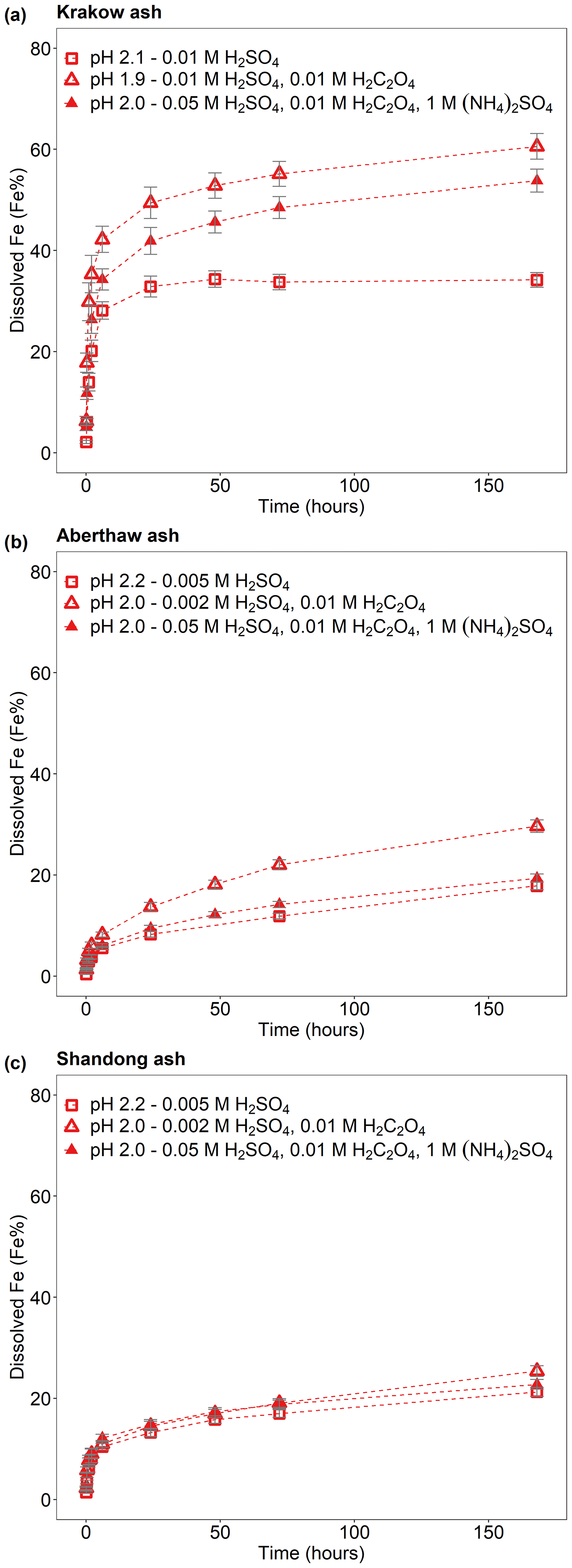
Figure 2Fe dissolution kinetics of (a) Krakow ash, (b) Aberthaw ash, and (c) Shandong ash in H2SO4 solutions at around pH 2 (red open rectangles), with 0.01 M H2C2O4 (red open triangles) and 1 M (NH4)2SO4 (red filled triangles). The molar concentrations of H2SO4, H2C2O4, and (NH4)2SO4 in the experiment solutions are shown. The final pH of the experiment solutions is also reported, which was calculated using the E-AIM III model for aqueous solutions (Wexler and Clegg, 2002) and accounting for the buffer capacity of the CFA samples (Experiments 1 and 3–4 at around pH 2). The data uncertainty was estimated using the error propagation formula.
The experimental treatment of dissolved Fe from Krakow ash in 0.05 H2SO4 solution with 1 M (NH4)2SO4 (Fig. 1a) resulted in a final predicted pH of 2.1. At that pH, the total Fe solubility of Krakow ash increased from 34 %, with no (NH4)2SO4, to 48 %, with a high (NH4)2SO4 concentration. The total Fe solubility of Krakow ash was around 28 % at pH 3.0 with 1 M (NH4)2SO4 (Fig. 1a), which is 3 times higher than that at pH 2.7 with no (NH4)2SO4. At around pH 2, the total Fe solubility of Aberthaw (Fig. 1b) and Shandong ash (Fig. 1c) increased by around 20 % and 30 % in the presence of (NH4)2SO4. By contrast, the total Fe solubility at pH 3.1 with 1 M (NH4)2SO4 was 7.5 % for Aberthaw ash (Fig. 1b) and 14 % for Shandong ash (Fig. 1c), respectively, which was between 4 and 7 times higher than in the experiments carried out at pH 2.9 without (NH4)2SO4.
The Fe dissolution of the CFA samples in H2SO4 solutions with 0.01 M H2C2O4 (at around pH 2) is shown in Fig. 2. The total Fe solubility of Krakow ash at pH 1.9 with 0.01 M H2C2O4 was 61 % (Fig. 2a), which was almost 2 times higher than that at pH 2.1 but without H2C2O4 (Fig. 2a). For Aberthaw ash, the oxalate contribution to the dissolution process led to a total Fe solubility of 30 % at pH 2.0 (Fig. 2b), which was 70 % higher than in the experiment carried out in 0.005 M H2SO4 (∼ pH 2.2; Fig. 2b). Shandong ash dissolution behaviour was not affected by the presence of oxalate (Fig. 2c).
We also investigated the effect of a high (NH4)2SO4 concentration on oxalate-promoted dissolution. In Fig. 2a, the total Fe solubility of Krakow ash decreased from 61 % at pH 1.9 in the presence of oxalate to 54 % at pH 2.0 with oxalate and (NH4)2SO4. For Aberthaw ash, the total Fe solubility at pH 2.0 decreased from 30 % in the presence of oxalate to 19 % after the addition of (NH4)2SO4 (Fig. 2b).
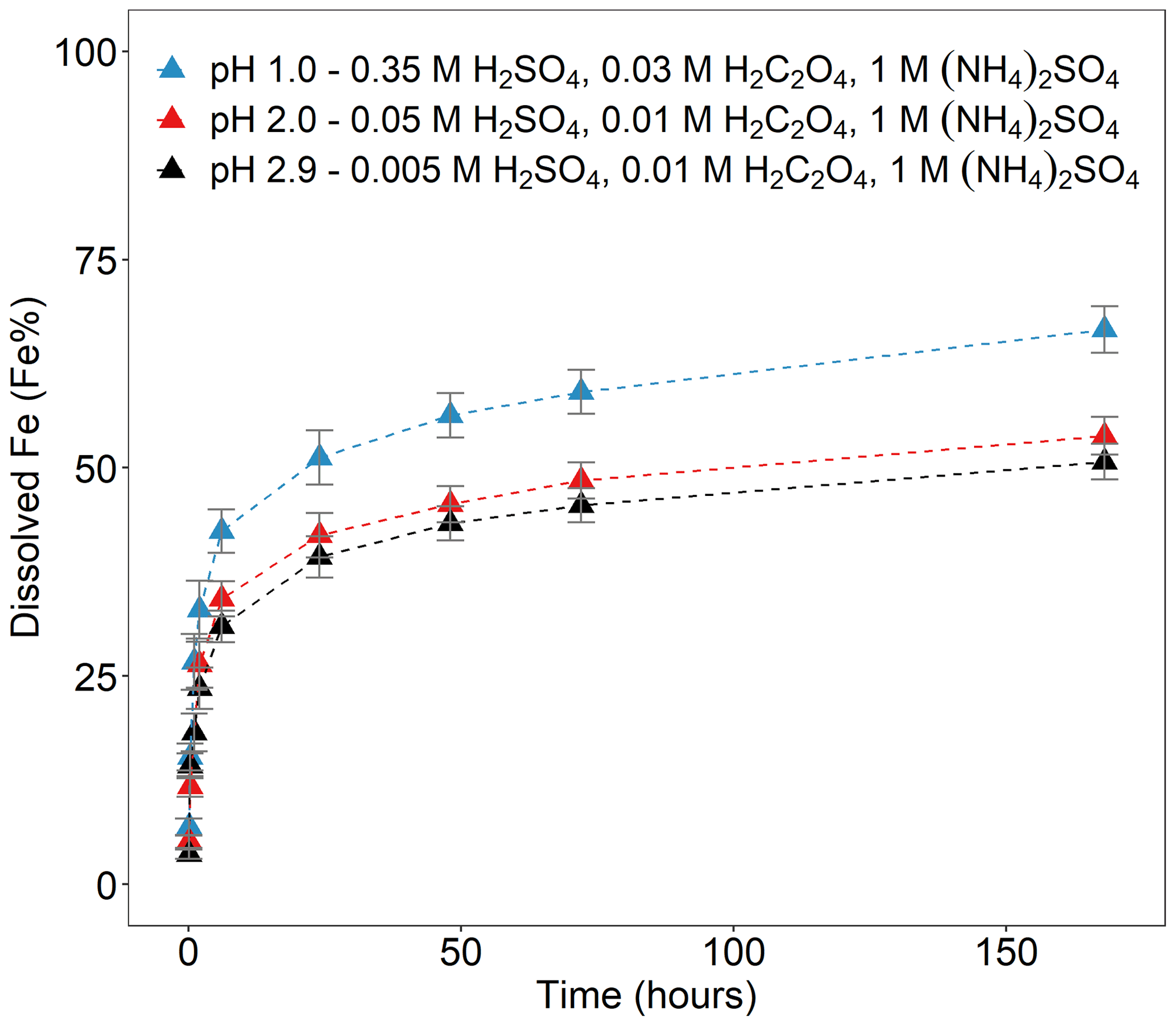
Figure 3Fe dissolution kinetics of Krakow ash in H2SO4 solutions at pH 1.0, with 0.03 M H2C2O4 and 1 M (NH4)2SO4 (blue filled triangles), at pH 2.0, with 0.01 M H2C2O4 and 1 M (NH4)2SO4 (red filled triangles), and at pH 2.9, with 0.01 M H2C2O4 and 1 M (NH4)2SO4 (black filled triangles). The molar concentrations of H2SO4, H2C2O4, and (NH4)2SO4 in the experiment solutions are shown. The final pH of the experiment solutions is also reported, which was calculated using the E-AIM III model for aqueous solutions (Wexler and Clegg, 2002) and accounting for the buffer capacity of the CFA samples (Experiment 7 at pH 1.0, Experiment 3 at pH 2.0, and Experiment 3 at pH 2.9 in Table S1). The data uncertainty was estimated using the error propagation formula.
Figure 3 shows the Fe dissolution behaviour of Krakow ash at different pH conditions in the presence of 1 M (NH4)2SO4 and H2C2O4 (0.01–0.03 M, depending on the solution pH). The total concentration of oxalate ions was calculated using the E-AIM model and was similar at different pH conditions, i.e. 0.015 at pH 1.0 (Experiment 7 in Table S3), 0.009 at pH 2.0, and 0.01 at pH 2.9 (Experiment 3 in Table S3). The highest total Fe solubility was observed at pH 1.0 (∼ 67 %). At pH 2.0, the total Fe solubility decreased to 54 %, and no substantial variations were observed between pH 2.0 and 2.9 (54 %–51 %). At pH 1.0, the concentration of H+ was considerably higher compared to pH 2.0–2.9, leading to a faster dissolution rate. The total concentration of oxalate ions was 1.5–1.6 times higher in the solution at pH 1.0 than at pH 2.0–2.9, which may also contribute to the faster dissolution rate. C2O concentration increased with rising pH. Although the concentration of H+ was lower at pH 2.9 than at pH 2.0, the E-AIM model estimated that C2O contributed around 35 % of the total oxalate concentration at pH 2.9, which was 4.5 times higher than at pH 2.0 (Experiment 3 in Table S3). The similar dissolution behaviour at pH 2.0 and 2.9 conditions may reflect the combination of these two opposite factors, with a higher concentration of C2O but lower concentration of H+ at pH 2.9 compared to 2.0.
We determined the Fe dissolution behaviour of Krakow ash at pH 1.0 in the presence of oxalate and increasing concentrations of (NH4)2SO4. The ash was leached in H2SO4 solutions, with 0.03 M H2C2O4 at pH 1.0, while the concentration of (NH4)2SO4 varied from 0 to 1.5 M. In Fig. 4, the total Fe solubility of Krakow ash in the presence of oxalate was 75 % at pH 1.0 and decreased to 68 % after the addition of 0.5 M (NH4)2SO4. Higher (NH4)2SO4 concentrations did not affect the Fe dissolution behaviour in the presence of oxalate at pH 1.0.
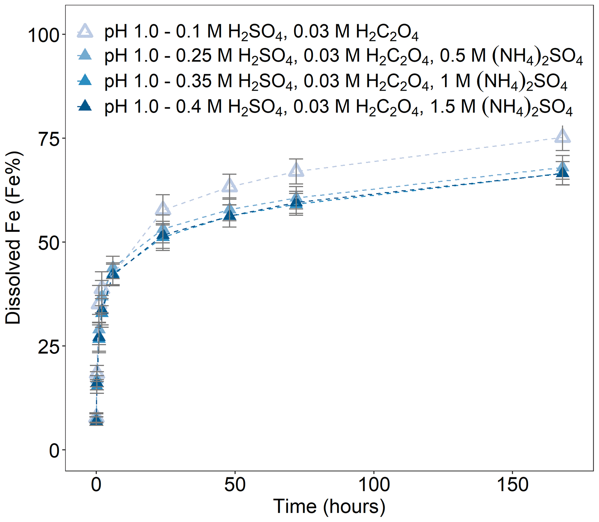
Figure 4Fe dissolution kinetics of Krakow ash in H2SO4 solutions at pH 1.0, with 0.03 M H2C2O4 and a concentration of (NH4)2SO4 from 0 to 1.5 M. The molar concentrations of H2SO4, H2C2O4, and (NH4)2SO4 in the experiment solutions are shown. The final pH of the experiment solutions is also reported, which was calculated using the E-AIM III model for aqueous solutions (Wexler and Clegg, 2002) and accounting for the buffer capacity of the CFA samples (Experiments 5–8 in Table S1). The data uncertainty was estimated using the error propagation formula.
3.2 Fe speciation
The Fe-bearing phases in the CFA samples determined through sequential extractions are shown in Fig. 5c. The Fe speciation in the Libyan dust precursor is added for comparison. Krakow ash had a total Fe (FeT) content of 5.2 %, while FeT in Aberthaw and Shandong ash was 3.1 % and 1.6 %, respectively. Amorphous Fe () was 6.5 % in Krakow ash, 2 % in Aberthaw ash, and 4.6 % in Shandong ash. The CFA samples showed very different dithionite Fe () content, 21.5 % in Krakow ash, 8 % in Aberthaw ash, and 14.8 % in Shandong ash. The content of magnetite () was considerably higher in Krakow ash (22.4 %) compared to Aberthaw (2.9 %) and Shandong (4.5 %) ash. About 50 %–87 % of Fe was contained in other phases, most likely in aluminosilicates. Overall, CFA had more magnetite and highly reactive amorphous Fe and less dithionite Fe than the Libyan dust precursor sample.
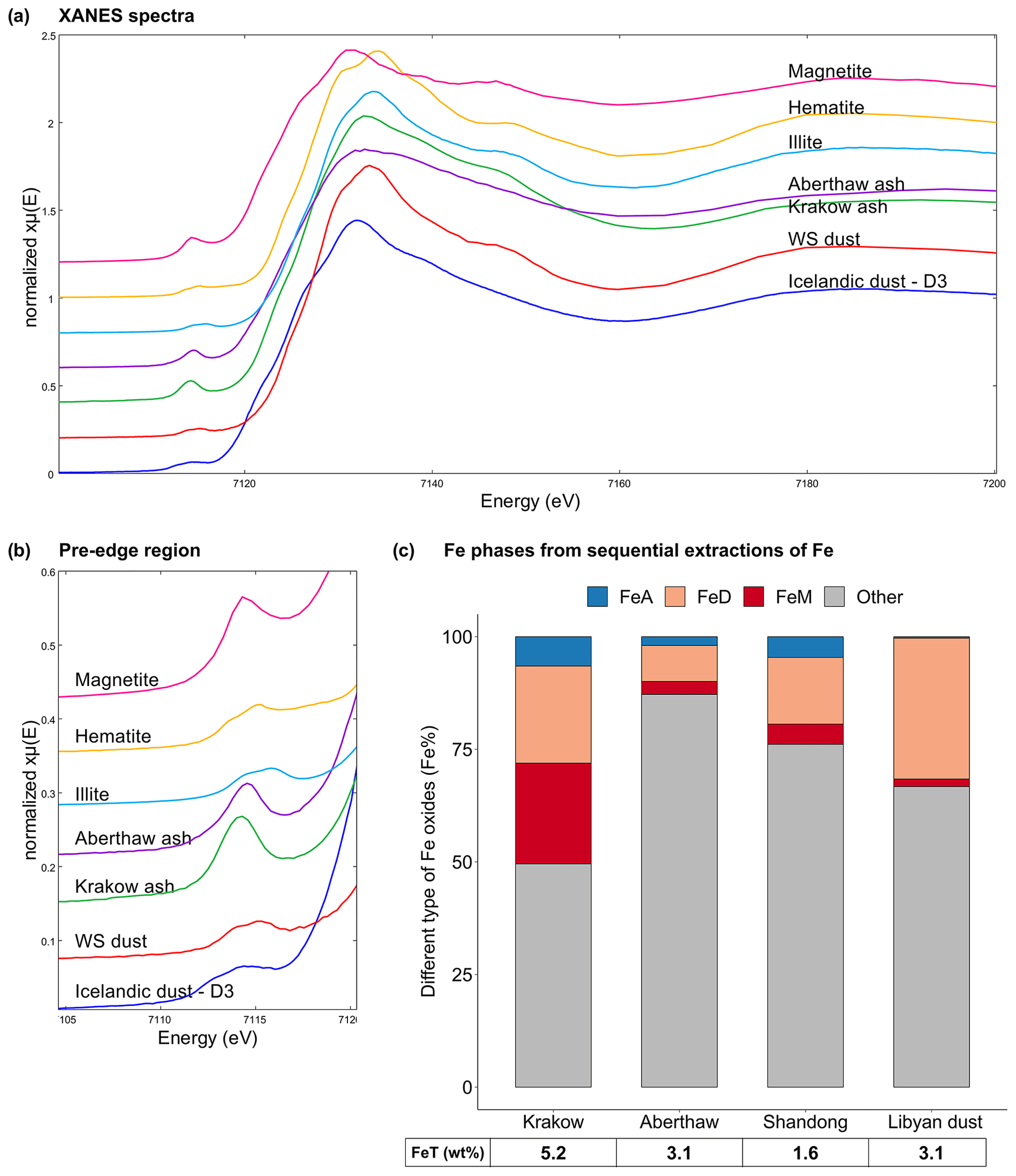
Figure 5Fe speciation in CFA and mineral dust samples. (a–b) Fe K-edge XANES spectra of Krakow ash, Aberthaw ash, magnetite, hematite, and illite standards, mineral dust from the Dyngjusandur dust hotspot in Iceland (D3 dust; Baldo et al., 2020), and mineral dust from western Sahara (WS dust; Shi et al., 2011b). (c) Percentages of ascorbate Fe (amorphous Fe, FeA), dithionite Fe (goethite/hematite, FeD), magnetite Fe (FeM), and other Fe (including Fe in aluminosilicates) to the total Fe (FeT) in the CFA samples and Libyan dust precursor. The FeT (as wt %) is given below each sample column. The data uncertainty was estimated using the error propagation formula, with 4 % for FeA/FeT, 11 % for FeD/FeT, 12 % for FeM/FeT, and 2 % for FeT.
In Fig. 5a–b, the Fe K-edge XANES spectra of Krakow and Aberthaw ash showed a single peak in the pre-edge region at around 7114.3 and 7114.6 eV, respectively. In the edge region, Aberthaw ash showed a broad peak at around 7132.2 eV, while the peak of Krakow ash was slightly shifted to 7132.9 eV and narrower. The pre-edge peak at around 7115.4 eV suggests that the Fe was mainly found as Fe(III). The spectral features of Aberthaw and Krakow ash are different from those of the hematite, magnetite, and illite standards, suggesting that the glass fraction was dominant and controlled their spectral characteristics, which is consistent with the results of the Fe sequential extractions. The XANES Fe K-edge spectra of the CFA samples have some common features with those of Icelandic dust but tend to differ from the mineral dust sourced in the Saharan dust source region. In the pre-edge region of the spectrum, Icelandic dust (sample D3 in Fig. 5a–b) showed a main peak at around 7114.4 eV and a second, less intense, peak at around 7112.7 eV, while a broad peak was observed at around 7131.9 eV in the edge region (Baldo et al., 2020). A mineral dust sample from the western Sahara (WS dust in Fig. 5a–b) showed a distinct double peak in the pre-edge region at around 7113.9 and 7115.2 eV and a main peak in the edge region at around 7133.3 eV (Baldo et al., 2020). The similarities between Icelandic ash and CFA could be because aluminium silicate glass is dominant in these samples (e.g. Baldo et al., 2020; Brown et al., 2011), while Fe-bearing phases in mineral dust from the Saharan region are primarily iron oxide minerals such as hematite and goethite, clay minerals, and feldspars (e.g. Shi et al., 2011b).
4.1 Fe dissolution scheme
Based on the laboratory experiments carried out on the CFA samples, we implemented a three-step dissolution scheme for proton-promoted and oxalate-promoted Fe dissolution (Table 1). The Fe dissolution kinetics were described as follows (Ito, 2015):
where RFei is the dissolution rate of individual mineral i, ki is the rate constant (mol Fe g−1 s−1), a(H+) is the H+ activity in solution, and mi represents the empirical reaction order for protons. The function fi () accounts for the suppression of mineral dissolution by competition for oxalate between surface Fe and dissolved Fe, as follows (Ito, 2015):
where [Fe] is the molar concentration (mol L−1) of Fe3+ dissolved in a solution, and [lig] is the molar concentration of a ligand (e.g. oxalate). fi was set to 1 for the proton-promoted dissolution.
Table 1Constants used to calculate Fe dissolution rates for fossil fuel combustion aerosols, based on laboratory experiments conducted at high ionic strength.
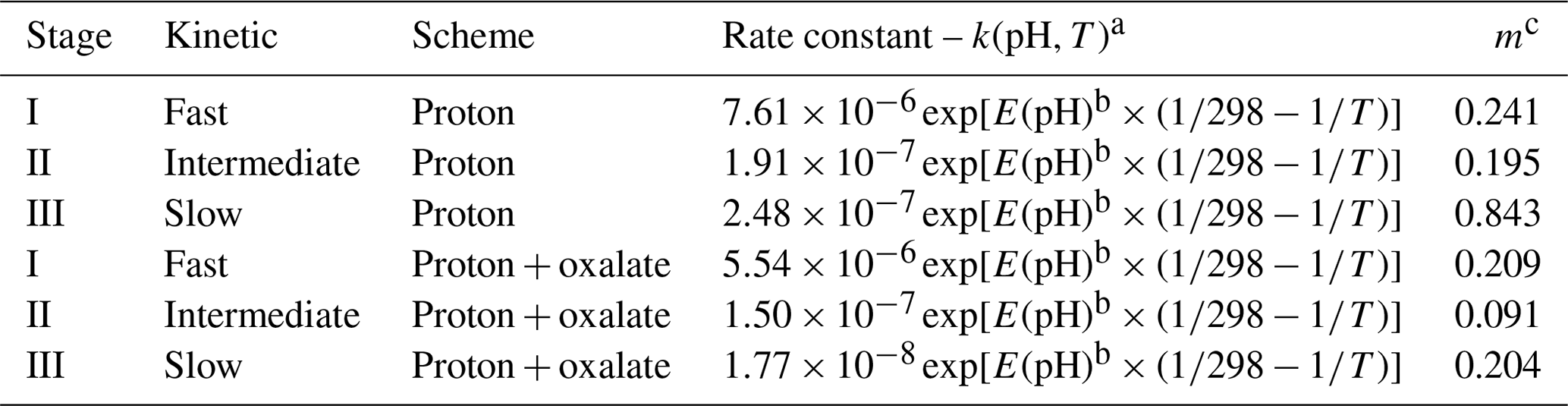
a k(pH,T) is the pH and temperature-dependent far-from-equilibrium rate constant (mol Fe g−1 s−1). The Fe dissolution scheme assumes three rate constants of fast, intermediate, and slow for the proton- and oxalate-promoted dissolution. The parameters were fitted to our measurements for Krakow ash. b . The parameters were fitted to the measurements for soils (Bibi et al., 2014). c m is the reaction order with respect to aqueous-phase protons, which was determined by a linear regression from our experimental data in the pH range between 2 and 3 for proton- and oxalate-promoted dissolution schemes.
The scheme assumes three rate constants, namely fast, intermediate, and slow, for the proton-promoted and the proton + oxalate-promoted dissolution (Table 1). These were obtained by fitting the parameters to our measurements for Krakow ash in H2SO4 and (NH4)2SO4 at pH 2–3, with and without oxalate (Experiments 2 and 3 in Table S1), which are shown in Fig. 6. The fast rate constant represents a highly reactive Fe species such as amorphous Fe oxyhydroxides, Fe carbonates, and Fe sulfates. The intermediate rate constant can be applied to nanoparticulate Fe oxides, while more stable phases including, for example, Fe aluminosilicate and crystalline Fe oxides have generally slower rates (Ito and Shi, 2016; Shi et al., 2011a, b, 2015). Similarly, we predicted the dissolution kinetics of Aberthaw ash and Shandong ash (Fig. 7). The dissolution kinetics of Krakow ash were calculated based also on the experimental results at pH 1.0, which are shown in Fig. S2 in comparison with kinetics predicted at pH 2.0 and pH 2.9 conditions.

Figure 6Comparison between the Fe dissolution kinetics of Krakow ash predicted using Eq. (1) and measured in H2SO4 solutions (a–b) with 1 M (NH4)2SO4 and (c–d) 0.01 M H2C2O4 and 1 M (NH4)2SO4. The molar concentrations of H2SO4, H2C2O4, and (NH4)2SO4 in the experiment solutions are shown. The final pH of the experiment solutions is also reported, which was calculated using the E-AIM III model for aqueous solutions (Wexler and Clegg, 2002) and accounting for the buffer capacity of the CFA samples (Experiments 2–3 in Table S1). The experiments conducted at around pH 2 are in red, while the experiments at around pH 3 are in black. The data uncertainty was estimated using the error propagation formula.
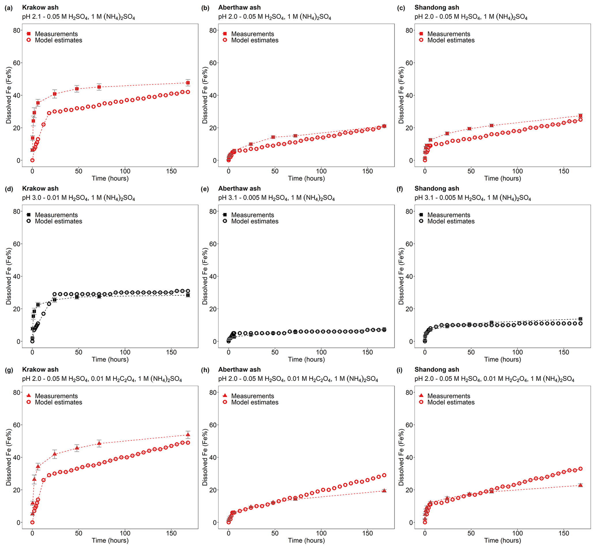
Figure 7Comparison between the Fe dissolution kinetics of Krakow, Aberthaw, and Shandong ashes predicted using Eq. (1) and measured in (a–c) H2SO4 solutions at around pH 2 with 1 M (NH4)2SO4 (Experiment 2 at around pH 2 in Table S1), (d–f) H2SO4 solutions at around pH 3 with 1 M (NH4)2SO4 (Experiment 2 at around pH 3 in Table S1), and (g–i) H2SO4 solutions at pH 2.0 with 0.01 M H2C2O4 and 1 M (NH4)2SO4 (Experiment 3 at pH 2.0 in Table S1). The molar concentrations of H2SO4, H2C2O4, and (NH4)2SO4 in the experiment solutions are shown. The final pH of the experiment solutions is also reported, which was calculated using the E-AIM III model for aqueous solutions (Wexler and Clegg, 2002) and accounting for the buffer capacity of the CFA samples.
The contribution of the oxalate-promoted dissolution to dissolved Fe was derived as the difference between the estimated dissolution rates for the proton + oxalate-promoted dissolution and the proton-promoted dissolution as follows:
The Fe dissolution rates were predicted at a wider range of pH, using Eqs. (1) and (3) and the parameters in Table 1, as follows:
Since RFei(oxalate) is less than 0 at low pH (<2), this equation applies to highly acidic conditions. As a result, the predicted amount of dissolved Fe was smaller when using the dissolution rate for the proton + oxalate-promoted dissolution, RFei(proton + oxalate), rather than the rate for the proton-promoted dissolution, RFei(proton), at pH < 2. Accordingly, the dissolution rate, RFei, was less dependent on the pH compared to RFei(proton) at highly acidic conditions, possibly due to the competition for the formation of surface complexes.
At pH > 2 when oxalate does promote Fe dissolution, the following equation applies:
4.2 Aerosol Fe solubility over the Bay of Bengal
The new dissolution scheme was applied in the IMPACT atmospheric chemistry transport model to predict the Fe solubility in atmospheric particles collected over the Bay of Bengal, which is an area for which there are detailed field measurements available (Bikkina et al., 2020; Kumar et al., 2010; Srinivas and Sarin, 2013; Srinivas et al., 2012) and multi-modelling analyses have been done (Ito et al., 2019). It, thus, represents a test for our experimental results in actual field conditions. A total of three sensitivity simulations were performed to explore the effects of the uncertainties associated with the dissolution schemes and mineralogical component of Fe. In addition, the former setting (Ito et al., 2021a) was used in the IMPACT model for comparison.
For all simulations, the total Fe emissions from anthropogenic combustion sources and biomass burning were estimated using the Fe emission inventory of Ito et al. (2018), including also emissions from the iron and steel industry, whereas Fe emissions from mineral dust sources were dynamically simulated (Ito et al., 2021a). In Test 0, we ran the model without the upgrades of the dissolution scheme discussed in Sect. 2.4 and additionally applied the photo-induced dissolution scheme for both combustion and dust aerosols (Ito, 2015; Ito and Shi, 2016), which was turned off in Test 1, Test 2, and Test 3 due to the lack of laboratory measurements under high ionic strength. To estimate the aerosol pH, we applied a H+ activity coefficient of 1 for Test 0, while the mean activity coefficient from Pye et al. (2020) was used for the other tests. The dissolution rate was assumed to be pH independent for highly acidic solutions (pH < 2; Ito, 2015) in Test 0, based on the laboratory measurements in Chen et al. (2012), while no pH threshold was considered in Test 1, Test 2, and Test 3, as the total dissolution (proton + oxalate) was suppressed at pH < 2 from the predicted dissolution rate.
In Test 1, we used the new dissolution scheme accounting for the proton- and oxalate-promoted dissolution of Krakow ash for all combustion aerosols in the model (Table 1). The dissolution kinetics were calculated using the base mineralogy for anthropogenic Fe emissions reported in Table S11 of Rathod et al. (2020). The Fe composition of wood was used for open biomass burning (Matsuo et al., 1992). In this simulation, three Fe pools were considered. Sulfate Fe in Rathod et al. (2020) was assumed to be fast pool, magnetite Fe as intermediate pool, and hematite, goethite, and clay as slow pool. In Test 2, we calculated the dissolution kinetics only considering the proton-promoted dissolution. In Test 3, the Fe pools were as determined here for Krakow ash, with ascorbate Fe (FeA) as fast pool, magnetite Fe (FeM) as intermediate pool, and hematite plus goethite Fe (FeD) and other Fe as slow pool (Fig. 5). FeA contains highly reactive Fe species with fast dissolution rates (Raiswell et al., 2008; Shi et al., 2011b). FeM appeared to work well for the different fly ash samples in the dissolution scheme as intermediate Fe pool. FeD is associated with crystalline Fe oxides which are mostly highly insoluble (Raiswell et al., 2008; Shi et al., 2011b), thus it was considered to be a slow pool in the dissolution scheme. We assumed other Fe to be mostly Fe-bearing aluminosilicates and considered this to be a slow Fe pool.
Observations of total Fe concentration and Fe solubility in PM2.5 along the cruise tracks over the Bay of Bengal for the period extending from 27 December 2008 to 26 January 2009 (Bikkina et al., 2020) were compared with temporally and regionally averaged data from model estimates. The daily averages of model results were calculated from hourly mass concentrations in the air over the surface ocean along the cruise tracks. The concentration of total Fe observed over the Bay of Bengal varies from 145 ± 144 ng m−3 over the northern Bay of Bengal (27 December 2008–10 January 2009) to 55 ± 23 ng m−3 over the southern Bay of Bengal (11–26 January 2009; Bikkina et al., 2020). In Fig. 8, the modelled concentrations of total Fe exhibit a similar variability to that of measurements with relatively higher values over the northern Bay of Bengal (59 ± 29 ng m−3 in different sensitivity simulations) compared to the southern Bay of Bengal (20 ± 12 ng m−3 in different sensitivity simulations). However, the modelled concentrations of total Fe were underestimated by a factor of 2.9 ± 1.5. The model reproduced the source apportion of Fe (Fig. 8; Table S4), which is qualitatively derived from previous observational studies, indicating that the concentrations of total Fe in aerosols over the northern Bay of Bengal are influenced by the emissions of dust and combustion sources from the Indo-Gangetic Plain (Kumar et al., 2010), whereas combustion sources (e.g. biomass burning and fossil-fuel) from southeastern Asia are dominant over the southern Bay of Bengal (Kumar et al., 2010; Srinivas and Sarin, 2013). On the other hand, the model could not reproduce the peak in the total Fe concentration (1.8 % of the Fe content in PM2.5 sample) reported around 29 December 2008. The total Fe observed in PM10 (430 ng m−3) on 29 December 2008 is lower than that measured on the day before (667 ng m−3) and the day after (773 ng m−3), whereas that in PM2.5 peaked on 29 December 2008 (Srinivas et al., 2012). Thus, the extreme value recorded only for PM2.5 on this date may be an outlier. But we do not have sufficient data to confirm this. One of the possibilities is that the sample collected aerosol particles from a mixture of different aerosols sources (e.g. dust and anthropogenic aerosols). This reflects one of the challenges of modelling such a dynamic parameter.
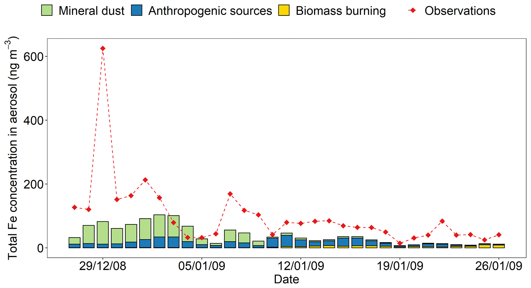
Figure 8Mass concentration of total Fe in PM2.5 aerosol particles over the Bay of Bengal from 27 December 2008 to 26 January 2009. Observations are from Bikkina et al. (2020; red filled diamonds). The concentrations of total Fe were calculated along the cruise tracks in the northern Bay of Bengal (27 December 2008–10 January 2009) and the southern Bay of Bengal (11–26 January 2009) using the IMPACT model. The total Fe emissions from anthropogenic combustion sources (ANTHRO) and biomass burning (BB) were estimated using the emission inventory of Ito et al. (2018), whereas Fe emissions from mineral dust sources (DUST) were dynamically simulated (Ito et al., 2021a).
The comparison of Fe solubility using the same total Fe emissions directly represents the effect of the new dissolution scheme on PM2.5. The aerosol Fe solubility measured over the southern Bay of Bengal is higher than that over the northern Bay of Bengal, respectively, with 32 % ± 11 % and 15 % ± 7 % (Bikkina et al., 2020), and model estimates showed a similar trend (Fig. 9). In Fig. 9 and Table S5, the calculated Fe solubilities over the northern Bay of Bengal in Test 1 (11 % ± 4 %), Test 2 (17 % ± 5 %), and Test 3 (17 % ± 6 %) were in good agreement with observations. The aerosol Fe solubility over the southern Bay of Bengal was better captured in Test 1 (30 % ± 5 %) and Test 3 (37 % ± 7 %), whereas Test 0 showed higher variability (37 % ± 22 %). The proton-promoted dissolution scheme in Test 2 significantly overestimated the Fe solubility over the Bay of Bengal (Fig. 9 and Table S5). The aerosol Fe solubility was largely overestimated in all scenarios after 22 January 2009, as open biomass burning sources become dominant (Fig. 8 and Table S4).
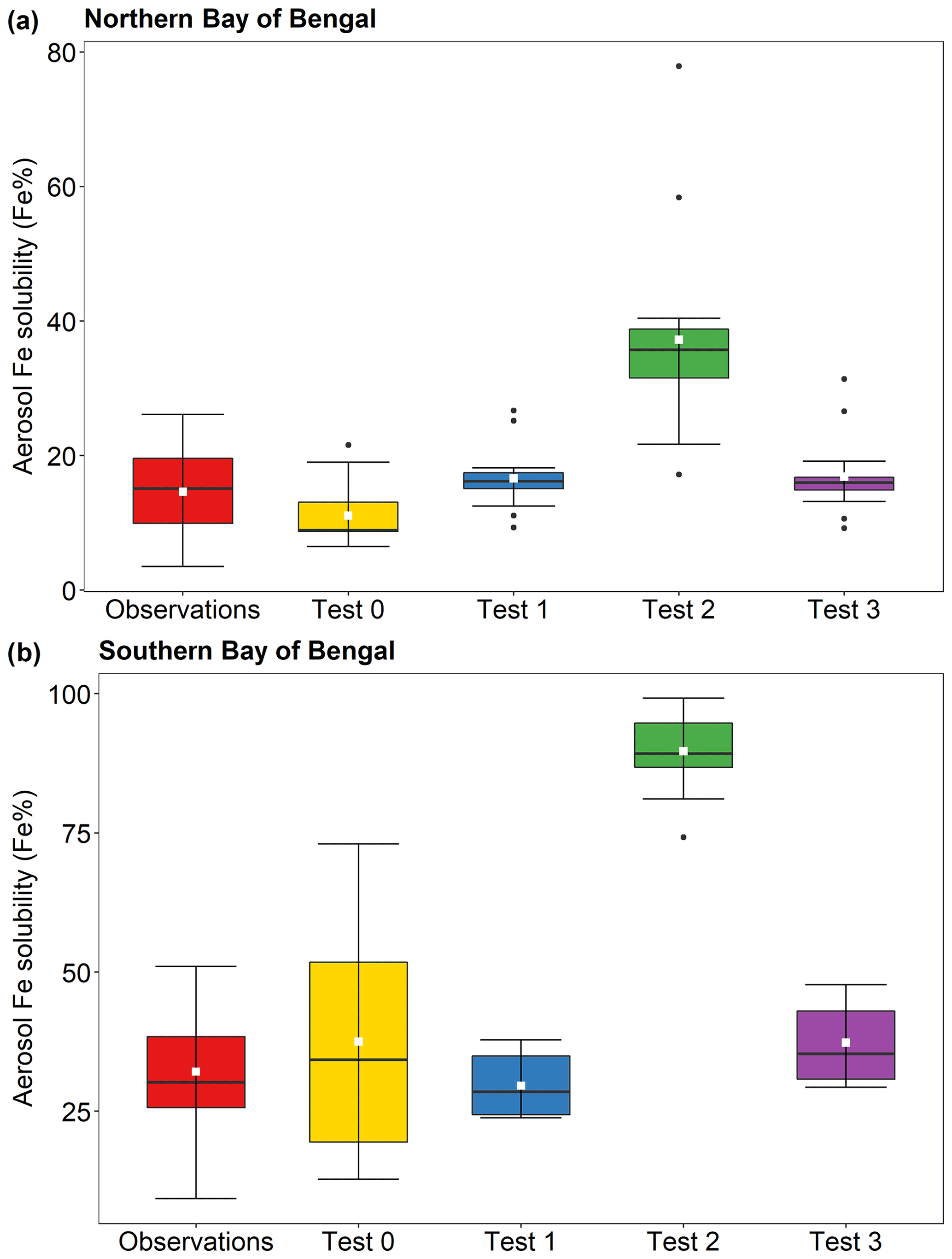
Figure 9Fe solubility in PM2.5 aerosol particles over (a) the northern Bay of Bengal, and (b) the southern Bay of Bengal from 27 December 2008 to 26 January 2009. Observations are from Bikkina et al. (2020). Model estimates of Test 0, Test 1, Test 2, and Test 3 were calculated along the cruise tracks using the IMPACT model. In Test 0, we run the model without upgrades (Ito et al., 2021a) and apply the proton-promoted, oxalate-promoted, and photoinduced dissolution schemes for combustion aerosols in Table S6 (Ito, 2015). The proton + oxalate dissolution scheme (Table 1) was applied in Tests 1 and 3, while proton-promoted dissolution is used for Test 2. We adopted the base mineralogy for anthropogenic Fe emissions (Rathod et al., 2020) in Tests 1 and 2. In Test 3, the Fe speciation of Krakow ash was used for all combustion sources. The small white square within the box shows the mean. The solid line within the box indicates the median. The lower and upper hinges correspond to the 25th and 75th percentiles. The whiskers above and below the box indicate the 1.5× interquartile range, and the data outside this range are plotted individually.
The comparison between observations and model predictions of aerosol Fe solubility over the Bay of Bengal is shown in Fig. S3. The agreement between the measurements and model predictions was the best in Test 1 and Test 3. These exhibited a good correlation with observations (R=0.49 in Test 1 and R=0.54 in Test 3), and the lowest root mean squared difference between the simulated and observed Fe solubilities (root mean square error (RMSE) equal to 11 in Test 1 and RMSE = 12 in Test 3). In Test 0, the model estimates showed a greater difference from observations (RMSE = 21) and poor correlation (R=0.26).
5.1 Dissolution behaviour of Fe in CFA
In this study, the Fe dissolution kinetics of CFA samples from the UK, Poland, and China were investigated under simulated atmospheric acidic conditions. A key parameter in both the atmosphere and the simulation experiments is the pH of the water interacting with the CFA particles. The lower the pH of the experimental solution, the faster the dissolution and eventually the higher the amount of Fe dissolved. Our results showed a strong pH dependence in low ionic strength conditions, with higher dissolution rates at lower pH. For example, reducing the solution pH from 2.7 to 2.1, the Fe solubility of Krakow ash in H2SO4 only increased by a factor of 4 (Fig. 1a) over the duration of the experiments, while the Fe solubility of Aberthaw and Shandong ash increased by 9–10 times from pH 2.9 to 2.2 (Fig. 1b–c). This enhancement is higher than that observed in studies conducted on mineral dust samples, which showed that one pH unit can lead to 3–4 times difference in dissolution rates (Ito and Shi, 2016; Shi et al., 2011a). Furthermore, Chen et al. (2012) reported that the Fe solubility of the certified CFA 2689 only increased by 10 % from pH 2 to 1, after 50 h of dissolution in acidic media. The Fe solubility of CFA (PM10 fractions) after 6 h at pH 2 was 6 %–10 % for Aberthaw and Shandong ash, respectively, and 28 % for Krakow ash (Fig. 1). The Fe in our CFA samples initially dissolved faster than the samples used by Fu et al. (2012), who reported 2.9 %–4.2 % Fe solubility in bulk CFA from three coal-fired power plants in China after 12 h leaching at pH 2. These results suggest that there are considerable variabilities in the pH-dependent dissolution of Fe in CFA. This could be due to differences in the Fe speciation between CFA samples and/or the different leaching media used.
Our results showed that high ionic strength has a major impact on the dissolution rates of CFA at low pH (i.e. pH 2–3). The Fe solubility of CFA increased by approximatively 20 %–40 % in the presence of 1 M (NH4)2SO4 at around pH 2 over the duration of the experiments and by a factor from 3 to 7 at around pH 3 conditions (Fig. 1). At high ionic strength, the activity of ions in solution is reduced; thus, in order to maintain similar pH conditions, the H+ concentration has to be increased (Table S1). Although Fe dissolution was primarily controlled by the concentration of H+, the high concentration of sulfate ions could also be an important factor contributing to Fe dissolution, particularly when the concentration of H+ in the system was low (e.g. pH 3). Previous research found that the high ability of anions to form soluble complexes with metals can enhance Fe dissolution (Cornell et al., 1976; Cornell and Schwertmann, 2003; Furrer and Stumm, 1986; Hamer et al., 2003; Rubasinghege et al., 2010; Sidhu et al., 1981; Surana and Warren, 1969). Sulfate ions adsorbed on the particles surface form complexes with Fe (e.g. Rubasinghege et al., 2010). This may increase the surface negative charge favouring the absorption of H+ and thereby increase Fe dissolution at the particle surface. In addition, the formation of surface complexes may weaken the bonds between Fe and the neighbouring ions (Cornell et al., 1976; Furrer and Stumm, 1986; Sidhu et al., 1981). Cwiertny et al. (2008) reported that, at pH 1–2, the high ionic strength generated by NaCl up to 1 M did not influence Fe dissolution of mineral dust particles. However, Ito and Shi (2016) showed that the high ionic strength resulting from the addition of 1 M (NH4)2SO4 in leaching solutions at pH 2–3 enhanced the Fe dissolution of dust particles, which was also observed here for the CFA samples. Borgatta et al. (2016) compared the Fe solubility of CFA from the USA Midwest, northeastern India, and Europe in an acidic solution (pH 1–2) containing 1 M NaCl. The Fe solubility measured after 24 h varied from 15 % to 70 % in different CFA (bulk samples) at pH 2 with 1 M NaCl, which was considerably higher than that observed at pH 2 with 1 M NaNO3 (<20 %; Kim et al., 2020). Both studies did not investigate the impact of ionic strength on the dissolution behaviour, i.e. by comparing the dissolution at low and high ionic strength. Note that both studies did not specify how the pH conditions were maintained at pH 2. Here, we considered the most important sources of high ionic strength in aerosol water and simulated Fe dissolution in the presence of (NH4)2SO4 and H2C2O4 under acidic conditions. We emphasize that the pH under high ionic strength here is estimated from a thermodynamic model, similar to those implemented in the IMPACT model.
The presence of oxalate enhanced the Fe dissolution in Krakow and Aberthaw ash at around pH 2 but not in Shandong ash (Fig. 2). The effect of oxalate on the Fe dissolution kinetics has also been studied by Chen and Grassian (2013) at pH 2 (11.6 mM H2C2O4). After 45 h of leaching, the Fe solubility of the certified CFA 2689 increased from 16 % in H2SO4 at pH 2 to 44 % in H2C2O4 at the same pH (Chen and Grassian, 2013). Therefore, the enhancement in the Fe solubility of CFA in the presence of the oxalate observed in this study (from no impact in Shandong ash to doubled dissolution in Krakow ash) is lower than the 2.8 times increase in Fe solubility reported for the certified CFA 2689 (Chen and Grassian, 2013). Since no data are available in Chen and Grassian (2013), we are unable to make a comparison with the other two certified CFA samples. The Fe solubility of Krakow ash after 48 h of leaching at pH 1.9 with 0.01 M H2C2O4 (Fig. 2a) was 53 %, which is within the range of Fe solubilities observed in Chen and Grassian (2013) for the certified CFA samples at similar pH and H2C2O4 concentrations (from 44 % to 78 %), whereas the Fe solubility of Aberthaw and Shandong ash (Fig. 2b–c; 18 %–17 % after 48 h of leaching at pH 2.0 with 0.01 M H2C2O4) was considerably lower than that of certified CFA (Chen and Grassian, 2013). These results suggest a large variability in the effects of oxalate on the Fe dissolution rates in different types of CFA.
Our results also indicated that high (NH4)2SO4 concentrations suppress oxalate-promoted Fe dissolution of CFA (Fig. 2), which was not considered in previous research. At pH 1.9 in the presence of oxalate, the Fe solubility of Krakow ash decreased by around 10 % after the addition of (NH4)2SO4, while the Fe solubility of Aberthaw ash decreased by 35 % (Fig. 2). We used the E-AIM model to estimate the concentration of oxalate ions and their activity (Table S3). The pH influences the speciation of H2C2O4 in the solution (e.g. Lee et al., 2007). H2C2O4 is the main species below pH 2, whereas HC2O is dominant between pH 2–4. Above pH 4, C2O is the principal species. In our experiments, H2C2O4 is mainly present as HC2O at around pH 2 (Experiments 3–4 in Table S3). In the presence of (NH4)2SO4, the activity coefficient of HC2O was reduced by approximatively 35 %–38 % (Experiments 3 in Table S3). Increasing the ionic strength lowers the activity of the oxalate ions, but at the same time favours the dissociation of the acid. At around pH 2 conditions, the E-AIM model estimated that the activity of C2O was reduced by around 1 order of magnitude in the presence of (NH4)2SO4, while its concentration increased 12–15 times (Experiments 3 in Table S3). The adsorption of anions can reduce the oxalate adsorption on the particle surface due to electrostatic repulsion, which results in slower release of Fe (Eick et al., 1999). The precipitation of ammonium hydrogen oxalate (NH4HC2O4) can also occur in the system, but this is very soluble and easily re-dissolves forming soluble oxalate species (Lee et al., 2007). We speculate that the high concentration of sulfate ions is likely to be responsible for inhibiting the oxalate-promoted dissolution by reducing the oxalate adsorption on the particle surface. At pH 1 in the presence of oxalate, increasing the concentration of (NH4)2SO4 from 0.5 to 1.5 M did not affect the Fe dissolution behaviour of the CFA samples (Fig. 4). As previously discussed, the adsorption of sulfate ions on the particle surface may inhibit oxalate-promoted dissolution. However, once the saturation coverage is reached, increasing the concentration of anions has no further effect on the dissolution rate (Cornell et al., 1976).
Fe speciation is an important factor affecting the Fe dissolution behaviour. CFA particles have very different chemical and physical properties depending, for example, on the nature of the coal burnt, the combustion conditions, the cooling process, and the particle control devices implemented at the power stations (e.g. Blissett and Rowson, 2012; Yao et al., 2015). This is likely the reason why the Fe speciation observed in the CFA samples analysed in this study from different locations varied considerably (Fig. 5). In the CFA samples, the Fe dissolution curves for different pH and ionic strengths generally showed the greatest rate of Fe release within the first 2 h, followed by a slower dissolution, reaching almost a plateau at the end of the experimental run. This indicates the presence of multiple Fe-bearing phases in CFA particles with a wide range of reactivity. Initially, highly reactive phases were the main contribution to dissolved Fe. As the dissolution continued, more refractory phases became the dominant source of dissolved Fe (Shi et al., 2011a). Scanning electron microscopy (SEM) analysis conducted on CFA samples showed that CFA particles are mostly spherical (e.g. Chen et al., 2012; Dudas and Warren, 1987; Valeev et al., 2018; Warren and Dudas, 1989), with Fe oxide aggregates on the surface (Chen et al., 2012; Valeev et al., 2018). The analysis of the CFA samples processed in aqueous solutions at low pH suggests that, initially, Fe dissolved from the reactive external glass coating (Dudas and Warren, 1987; Warren and Dudas, 1989) and from the Fe oxide aggregates on the particle surface (Chen et al., 2012; Valeev et al., 2018). Subsequently, Fe is likely realized from the structure of the aluminium silicate glass (Chen et al., 2012; Dudas and Warren, 1987; Valeev et al., 2018; Warren and Dudas, 1989) and crystalline Fe oxide phases (Warren and Dudas, 1989). Overall, Krakow ash showed the fastest dissolution rates, but the dissolution of highly reactive Fe species as FeA is insufficient to account for the high Fe solubility observed at low pH. Our results showed that once the FeA dissolved, additional Fe was dissolved from more refractory Fe-bearing phases. The modelled dissolution kinetics obtained using FeM as intermediate pool were in good agreement with the measurements (Figs. 7 and S2). FeM is likely to be primary magnetite but may contain a fraction of the more reactive aluminosilicate glass. Our model results suggest that magnetite in CFA particles may be more soluble than shown in Marcotte et al. (2020). It is possible that, in real CFA samples, the physicochemical properties of minerals, including, for example, crystal size, degree of crystallinity, cationic, and anionic substitution in the lattice which influence the Fe dissolution behaviour (e.g. Schwertmann, 1991), are likely to be different from those of the reference minerals analysed in Marcotte et al. (2020). In order to investigate the links between Fe solubility and Fe speciation/mineralogy, more work is needed to determine the Fe mineralogy in CFA samples at emission and after atmospheric processing in combination with solubility experiments.
Finally, the modelled dissolution kinetics obtained using the new dissolution scheme for CFA (Table 1) showed better agreement with laboratory measurements than when using the original scheme (Ito, 2015; Fig. 10). In Fig. 10a–b, we compared the Fe dissolution kinetics of Krakow ash at around pH 2 and 3 with 1 M (NH4)2SO4, which was calculated using the proton-promoted dissolution scheme in Table 1 with the dissolution kinetics calculated at similar pH but using the proton-promoted dissolution scheme for combustion aerosols in Ito (2015; Table S6). The dissolution scheme in Ito (2015) was based on laboratory measurements conducted at low ionic strength (Chen et al., 2012) and assumed a single Fe-bearing phase in combustion aerosol particles, while the new dissolution scheme considered the high ionic strength of aerosol water and assumed three rate constants for the fast, intermediate, and slow kinetics of the different Fe-bearing phases present in CFA particles. The Fe dissolution kinetics obtained using the new dissolution scheme showed a better agreement with measurements and was enhanced compared to the model estimates obtained using the original dissolution scheme (Ito, 2015) for low ionic strength conditions (Fig. 10a–b). Figure 10c–d show the Fe dissolution kinetics of Krakow ash at pH 2.0 and 2.9, with 0.01 M H2C2O4 and 1 M (NH4)2SO4, calculated using the proton- and oxalate-promoted dissolution scheme in Table 1 and the dissolution kinetics calculated at a similar pH and H2C2O4 concentration but using the scheme in Ito (2015; i.e. single-phase dissolution; see Table S6). The Fe dissolution kinetics predicted using the new dissolution scheme had a much better agreement with measurements. Figure 10e shows the suppression of the oxalate-promoted dissolution at pH 2.0 and high (NH4)2SO4 concentrations. At pH 2, the proton-promoted dissolution was comparable to the proton + oxalate-promoted dissolution (Fig. 10e), with RFe(oxalate) close to zero (see Eq. 3). At pH 2.9, the proton + oxalate-promoted dissolution was higher than the proton + oxalate-promoted dissolution (Fig. 10f), with RFe(oxalate) > 0 (Eq. 5).
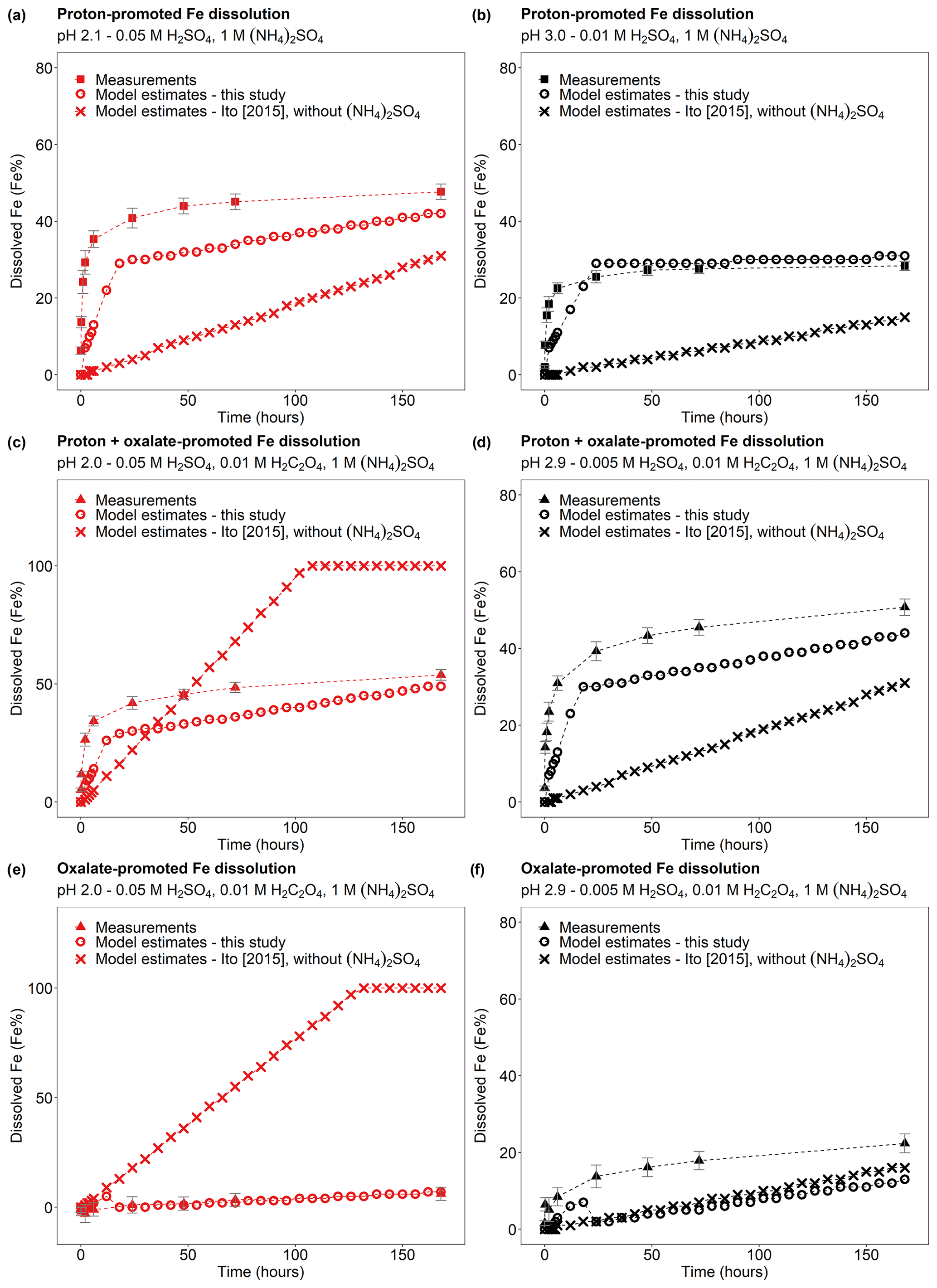
Figure 10Comparison between the Fe dissolution kinetics of Krakow ash calculated using the original (Ito, 2015) and the new dissolution scheme (Tables 1 and S6). (a–b) Proton-promoted Fe dissolution in H2SO4 solutions with 1 M (NH4)2SO4 at pH 2.1 (a) and at pH 3.0 (b) (Experiment 2 at pH 2.1 and Experiment 2 at pH 3.0 in Table S1). (c–d) Proton + oxalate-promoted Fe dissolution in H2SO4 solutions, with 0.01 M H2C2O4 and 1 M (NH4)2SO4 at pH 2.0 (c), and at pH 2.9 (d) (Experiment 3 at pH 2.0 and Experiment 3 at pH 2.9 in Table S1). The Fe dissolution kinetics were predicted using the rate constants in Table 1 calculated in this study (open circles) and the dissolution scheme for combustion aerosols in Ito (2015; cross marks). Note that the dissolution scheme in Ito (2015) was calculated based on laboratory measurements conducted at low ionic strength. (e–f) Contribution of the oxalate-promoted dissolution to dissolved Fe estimated using Eq. (3). The molar concentrations of H2SO4, H2C2O4, and (NH4)2SO4 in the experiment solutions are shown. The final pH of the experiment solutions is also reported, which was calculated using the E-AIM III model for aqueous solutions (Wexler and Clegg, 2002) and accounting for the buffer capacity of the CFA samples.
Moreover, the new three-step dissolution scheme better captured the initial fast dissolution of CFA (Fig. 10), which was also observed in previous research (Borgatta et al., 2016; Chen et al., 2012; Chen and Grassian, 2013; Fu et al., 2012; Kim et al., 2020; except for the certified CFA 2689 in Chen et al., 2012, which showed increasing dissolution rates over the duration of the experiment). Furthermore, the new scheme enabled us to account for the different Fe speciation determined in the CFA samples, which could be a key factor contributing to the different Fe dissolution behaviour observed in the present study and in the literature (Borgatta et al., 2016; Chen et al., 2012; Chen and Grassian, 2013; Fu et al., 2012; Kim et al., 2020). In Fig. 7, the dissolution kinetics of Aberthaw and Shandong ash calculated using the dissolution rates in Table 1 and the Fe-bearing phases determined in the samples showed a good agreement with the measurements.
5.2 Comparison with mineral dust
High ionic strength also impacted the dissolution rates of the Libyan dust precursor sample at low pH (Fig. S4). At around pH 2 conditions, the proton-promoted Fe dissolution of Libyan dust was enhanced by ∼ 40 % after the addition of (NH4)2SO4. At around pH 2 and with 0.01 M H2C2O4, the Fe solubility of Libyan dust decreased by ∼ 30 % in the presence of (NH4)2SO4. Overall, the Fe solubility of Libyan dust was lower compared to that observed in the CFA samples. After 168 h of leaching at pH 2.1, with 1 M (NH4)2SO4, the Fe solubility of Libyan dust was 7.2 % (Fig. S4), which was from around 3 to 7 times lower compared to that of the CFA samples (Fig. 1). At around pH 2 conditions in the presence of oxalate and high (NH4)2SO4 concentration, the Fe solubility of Libyan dust rose to ∼ 13.6 % (Fig. S4), which is still 4 times lower than that of Krakow ash and around 1.5 lower than Aberthaw and Shandong ash (Fig. 2). The Fe solubilities of the Libyan dust observed in this study are comparable with those of the Tibesti dust (Tibesti Mountains, Libya; 25.583333∘ N, 16.516667∘ E) in Ito and Shi (2016) at similar experimental conditions.
The enhanced Fe solubility in CFA compared to mineral dust could be primarily related to the different Fe speciation (Fig. 5). CFA contained more highly reactive Fe and magnetite but less hematite and goethite than mineral dust.
Although mineral dust is the largest contribution to aerosol Fe while CFA accounts for only a few percent, the atmospheric processing of CFA may result in a larger-than-expected contribution of bio-accessible Fe deposited to the surface ocean. It is, thus, important to quantify the amount and nature of CFA in atmospheric particles.
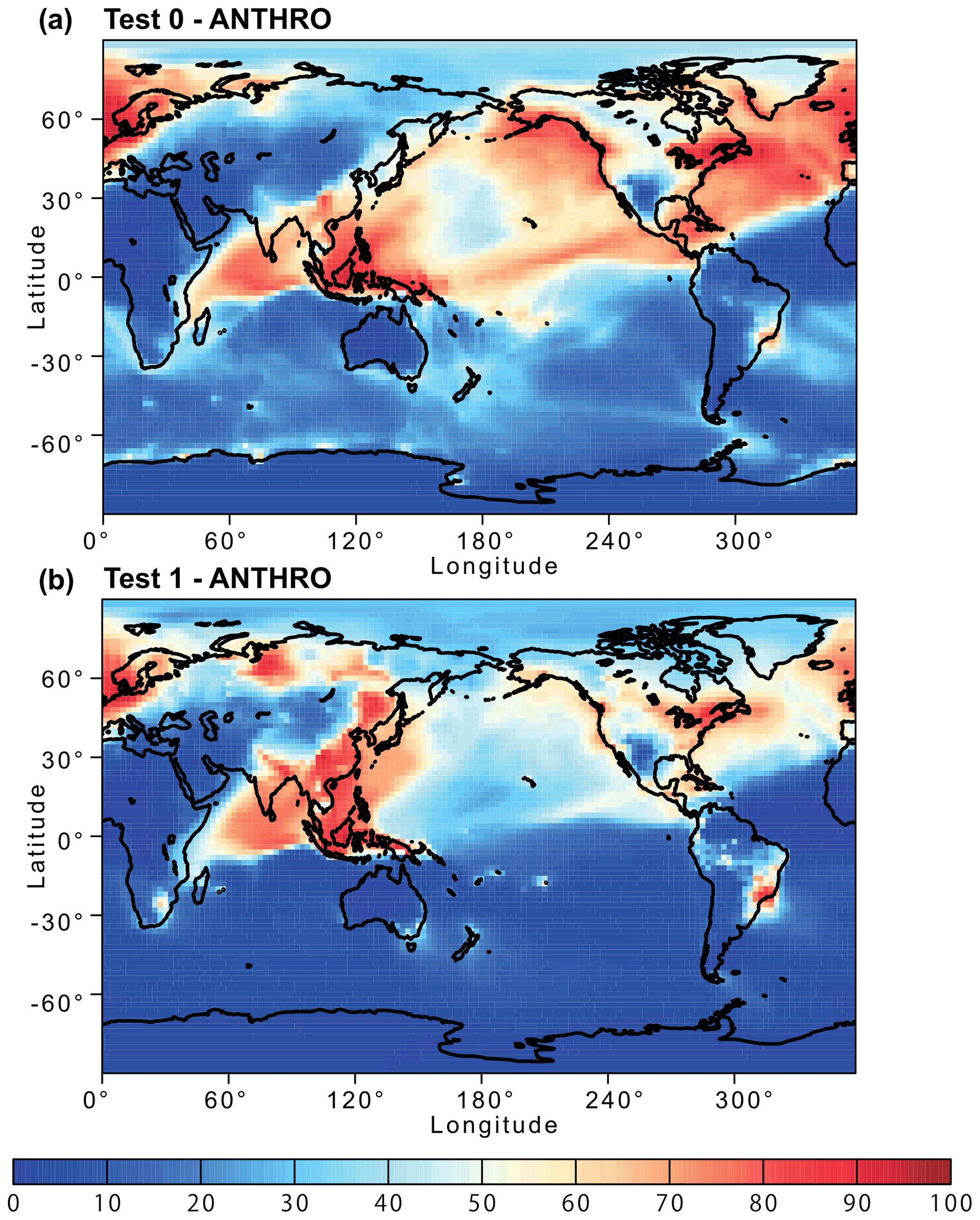
Figure 11Percentage contribution of anthropogenic combustion (ANTHRO) aerosol to the atmospheric dissolved Fe concentration near the ground surface from (a) Test 0 and (b) Test 1 for December 2008 and January 2009. In Test 0, we ran the model without upgrades in the Fe dissolution scheme (Ito et al., 2021a) and applied the proton-promoted, oxalate-promoted, and photoinduced dissolution schemes for combustion aerosols in Table S6 (Ito, 2015). The proton + oxalate dissolution scheme (Table 1) was applied in Test 1, and we adopted the base mineralogy for anthropogenic Fe emissions (Rathod et al., 2020).
5.3 Comparison of modelled Fe solubility with field measurements
The model results obtained using the new dissolution scheme for the proton + oxalate-promoted dissolution (Table 1) in Test 1 and Test 3 provided a better estimate of aerosol Fe solubility over the Bay of Bengal than the other tests (Figs. 9 and S3). At the same time, the new model improved the agreement of aerosol Fe solubility from Test 0 (68 % ± 5 %) to Test 1 (35 % ± 2 %) and Test 3 (47 % ± 1 %) with the field data (25 % ± 3 %) but still overestimated it after 22 January 2009, when open biomass burning sources become dominant (Bikkina et al., 2020), as also shown in Fig. 8 and Table S4. This could be due to the unrepresentative Fe speciation used in Test 1 and Test 3 for biomass burning over the Bay of Bengal. To reduce the uncertainty in model predictions, emission inventories could be improved through a comprehensive characterization of Fe species in combustion aerosol particles.
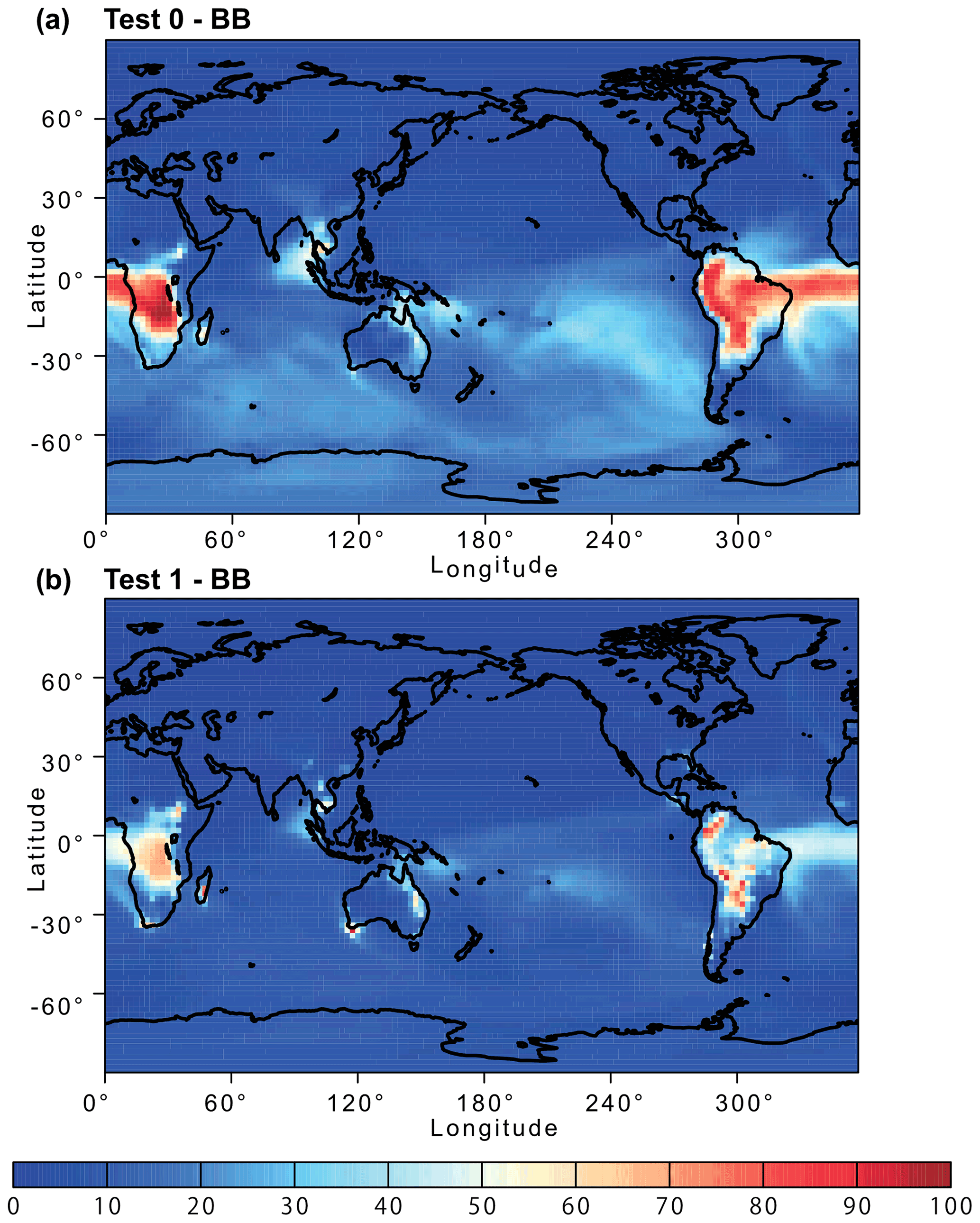
Figure 12Percentage contribution of biomass burning (BB) aerosol to the atmospheric dissolved Fe concentration near the ground surface from (a) Test 0 and (b) Test 1 for December 2008 and January 2009. In Test 0, we ran the model without upgrades in the Fe dissolution scheme (Ito et al., 2021a) and applied the proton-promoted, oxalate-promoted, and photoinduced dissolution schemes for combustion aerosols in Table S6 (Ito, 2015). The proton + oxalate dissolution scheme (Table 1) was applied in Test 1, and we adopted the base mineralogy for anthropogenic Fe emissions (Rathod et al., 2020).
The revised model also enabled us to predict sensitivity to a more dynamic range of pH changes, particularly between anthropogenic combustion and biomass burning by the suppression of the oxalate-promoted dissolution at pH lower than 2. In Test 0, the dissolution rate was assumed to be independent from the pH for extremely acidic solutions (pH < 2). The results show that the proton-promoted dissolution scheme in Test 2 significantly overestimated aerosol Fe solubility (Figs. 9 and S3), which indicates the suppression of the proton + oxalate-promoted dissolution at pH < 2. In Fig. S5, the model estimates of aerosol Fe solubility over the Bay of Bengal considerably improved in Test 1 (RMSE 11) compared to Test 0 (RMSE 21), but more work is needed to improve size-resolved Fe emission, transport, and deposition. The model results in Test 1 indicate a larger contribution of anthropogenic combustion sources to the atmospheric Fe loading over East Asia (Fig. 11) but a smaller contribution of biomass burning sources downwind from tropical regions (Fig. 12). We demonstrated that the implementation of the new Fe dissolution scheme, including a rapid Fe release at the initial stage and highly acidic conditions, enhanced the model estimates. However, in Test 1, we turned off the photo-reductive dissolution scheme (Ito, 2015) which was based on the laboratory measurements in Chen and Grassian (2013). To determine the photoinduced dissolution kinetics of CFA particles, it is necessary to account for the effect of high concentration of (NH4)2SO4 on photo-reductive dissolution rate, which should be considered in future research.
The new dissolution schemes for the proton-promoted and oxalate-promoted dissolution are reported in Table 1. Table S1 reports the concentrations of H2SO4, H2C2O4, and (NH4)2SO4 in the experiment solutions, the original and final pH from model estimates (including H+ concentrations and activities), and the pH measurements for the solution with low ionic strength. Table S3 contains the summary of the concentration and activity of total oxalate ions, C2O, and HC2O in the experiment solutions calculated using the E-AIM III model. The observations of the mass concentration of total Fe, dissolved Fe, and Fe solubility for the fine mode (PM2.5) over the Bay of Bengal are from Bikkina et al. (2020) and are available at https://doi.org/10.1021/acsearthspacechem.0c00063. The modelled mass concentrations of total Fe in aerosol particles and the aerosol Fe solubilities over the Bay of Bengal are reported in Tables S4 and S5, respectively. The Fe speciation, the measurements of the Fe dissolution kinetics, and the results of the IMPACT model for each sensitivity simulation (Test 0–3) can be downloaded at https://doi.org/10.25500/edata.bham.00000702 (Baldo, 2022).
The supplement related to this article is available online at: https://doi.org/10.5194/acp-22-6045-2022-supplement.
CB, ZS, and AI designed the experiments and discussed the results. ZS supervised the experimental and data analyses. CB conducted the experiments and the data analysis with contributions from ZS, AI, MDK, and NDa. NDa, ZS, and KI performed the XANES measurements. AI developed the model of the dissolution kinetics and performed the model simulations. Krakow and Aberthaw ash were provided by TJ, while Shandong ash was provided by WL. Soil 5 from Libya was collected by NDr. CB prepared the article, with contributions from MDK and all the other co-authors.
The contact author has declared that neither they nor their co-authors have any competing interests.
Publisher's note: Copernicus Publications remains neutral with regard to jurisdictional claims in published maps and institutional affiliations.
We acknowledge Diamond Light Source for the time on Beamline/Lab I18 under various proposals (SP22244-1, SP12760-1, and SP10327-1). We are grateful to Srinivas Bikkina, Manmohan Sarin, and their colleagues, for kindly providing the observational data set during the SK-254 cruise, supported by the Geosphere–Biosphere programme funded by the Indian Space Research Organization (Bengaluru, India).
Clarissa Baldo has been funded by the Natural Environment Research Council (NERC) CENTA studentship (grant no. NE/L002493/1). Support for this research was provided to Akinori Ito by JSPS KAKENHI (grant no. 20H04329) and the Integrated Research Program for Advancing Climate Models (TOUGOU; grant no. JPMXD0717935715) from the Ministry of Education, Culture, Sports, Science and Technology (MEXT), Japan.
This paper was edited by Ari Laaksonen and reviewed by Rachel Shelley and Morgane Perron.
Baker, A. R., Li, M., and Chance, R.: Trace Metal Fractional Solubility in Size-Segregated Aerosols From the Tropical Eastern Atlantic Ocean, Global Biogeochem., 34, e2019GB006510, https://doi.org/10.1029/2019GB006510, 2020.
Baker, A. R., Kanakidou, M., Nenes, A., Myriokefalitakis, S., Croot, P. L., Duce, R. A., Gao, Y., Guieu, C., Ito, A., Jickells, T. D., Mahowald, N. M., Middag, R., Perron, M. M. G., Sarin, M. M., Shelley, R., and Turner, D. R.: Changing atmospheric acidity as a modulator of nutrient deposition and ocean biogeochemistry, Sci. Adv., 7, eabd8800, https://doi.org/10.1126/sciadv.abd8800, 2021.
Baldo, C.: Research data supporting “Iron from coal combustion particles dissolves much faster than mineral dust under simulated atmospheric acidic conditions”, University of Birmingham [data set], https://doi.org/10.25500/edata.bham.00000702, 2022.
Baldo, C., Formenti, P., Nowak, S., Chevaillier, S., Cazaunau, M., Pangui, E., Di Biagio, C., Doussin, J.-F., Ignatyev, K., Dagsson-Waldhauserova, P., Arnalds, O., MacKenzie, A. R., and Shi, Z.: Distinct chemical and mineralogical composition of Icelandic dust compared to northern African and Asian dust, Atmos. Chem. Phys., 20, 13521–13539, https://doi.org/10.5194/acp-20-13521-2020, 2020.
Bibi, I., Singh, B., and Silvester, E.: Dissolution kinetics of soil clays in sulfuric acid solutions: Ionic strength and temperature effects, Appl. Geochem., 51, 170–183, https://doi.org/10.1016/j.apgeochem.2014.10.004, 2014.
Bikkina, S., Kawamura, K., Sarin, M., and Tachibana, E.: 13C Probing of Ambient Photo-Fenton Reactions Involving Iron and Oxalic Acid: Implications for Oceanic Biogeochemistry, ACS Earth Space Chem., 4, 964–976, https://doi.org/10.1021/acsearthspacechem.0c00063, 2020.
Blissett, R. S. and Rowson, N. A.: A review of the multi-component utilisation of coal fly ash, Fuel, 97, 1–23, https://doi.org/10.1016/j.fuel.2012.03.024, 2012.
Borgatta, J., Paskavitz, A., Kim, D., and Navea, J. G.: Comparative evaluation of iron leach from different sources of fly ash under atmospherically relevant conditions, Environ. Chem., 13, 902–912, https://doi.org/10.1071/en16046, 2016.
Boyd, P. W., Jickells, T., Law, C. S., Blain, S., Boyle, E. A., Buesseler, K. O., Coale, K. H., Cullen, J. J., de Baar, H. J. W., Follows, M., Harvey, M., Lancelot, C., Levasseur, M., Owens, N. P. J., Pollard, R., Rivkin, R. B., Sarmiento, J., Schoemann, V., Smetacek, V., Takeda, S., Tsuda, A., Turner, S., and Watson, A. J.: Mesoscale Iron Enrichment Experiments 1993–2005: Synthesis and Future Directions, Science, 315, 612–617, https://doi.org/10.1126/science.1131669, 2007.
British Petroleum (BP): Statistical Review of World Energy 2020, https://www.bp.com/en/global/corporate/energy-economics/statistical-review-of-world-energy.html, (last access: 10 April 2021), 2020.
Brown, P., Jones, T., and BéruBé, K.: The internal microstructure and fibrous mineralogy of fly ash from coal-burning power stations, Environ. Pollut., 159, 3324–3333, https://doi.org/10.1016/j.envpol.2011.08.041, 2011.
Chen, H. H. and Grassian, V. H.: Iron Dissolution of Dust Source Materials during Simulated Acidic Processing: The Effect of Sulfuric, Acetic, and Oxalic Acids, Environ. Sci. Technol., 47, 10312–10321, https://doi.org/10.1021/es401285s, 2013.
Chen, H., Laskin, A., Baltrusaitis, J., Gorski, C. A., Scherer, M. M., and Grassian, V. H.: Coal fly ash as a source of iron in atmospheric dust, Environ. Sci. Technol., 46, 2112–2120, https://doi.org/10.1021/es204102f, 2012.
Cornell, R. M. and Schwertmann, U.: The Iron Oxides: Structure, Properties, Reactions, Occurrence and Uses, Wiley-VCH, New York, ISBN 3-527-30274-3, 2003.
Cornell, R. M., Posner, A. M., and Quirk, J. P.: Kinetics and mechanisms of the acid dissolution of goethite (α-FeOOH), Journal of Inorganic and Nuclear Chemistry, 38, 563–567, https://doi.org/10.1016/0022-1902(76)80305-3, 1976.
Cwiertny, D. M., Baltrusaitis, J., Hunter, G. J., Laskin, A., Scherer, M. M., and Grassian, V. H.: Characterization and acid-mobilization study of iron-containing mineral dust source materials, J. Geophys. Res.-Atmos, 113, D05202, https://doi.org/10.1029/2007jd009332, 2008.
Dudas, M. J. and Warren, C. J.: Submicroscopic model of fly ash particles, Geoderma, 40, 101–114, https://doi.org/10.1016/0016-7061(87)90016-4, 1987.
Eick, M. J., Peak, J. D., and Brady, W. D.: The Effect of Oxyanions on the Oxalate-Promoted Dissolution of Goethite, Soil Sci. Soc. Am. J., 63, 1133–1141, https://doi.org/10.2136/sssaj1999.6351133x, 1999.
Emerson, E. W., Hodshire, A. L., DeBolt, H. M., Bilsback, K. R., Pierce, J. R., McMeeking, G. R., and Farmer, D. K.: Revisiting particle dry deposition and its role in radiative effect estimates, P. Natl. Acad. Sci. USA, 117, 26076–26082, https://doi.org/10.1073/pnas.2014761117, 2020.
Fu, H., Cwiertny, D. M., Carmichael, G. R., Scherer, M. M., and Grassian, V. H.: Photoreductive dissolution of Fe-containing mineral dust particles in acidic media, J. Geophys. Res., 115, D11304, https://doi.org/10.1029/2009jd012702, 2010.
Fu, H. B., Lin, J., Shang, G. F., Dong, W. B., Grassian, V. H., Carmichael, G. R., Li, Y., and Chen, J. M.: Solubility of Iron from Combustion Source Particles in Acidic Media Linked to Iron Speciation, Environ. Sci. Technol., 46, 11119–11127, https://doi.org/10.1021/es302558m, 2012.
Furrer, G. and Stumm, W.: The coordination chemistry of weathering: I. Dissolution kinetics of δ-Al2O3 and BeO, Geochim. Cosmochim. Ac.,, 50, 1847–1860, https://doi.org/10.1016/0016-7037(86)90243-7, 1986.
Hamer, M., Graham, R. C., Amrheim, C., and Bozhilov, K. N.: Dissolution of ripidolite (Mg, Fe-chlorite) in organic and inorganic acid solutions, Soil Sci. Soc. Am. J., 67, 654–661, https://doi.org/10.2136/sssaj2003.6540, 2003.
Ito, A.: Atmospheric Processing of Combustion Aerosols as a Source of Bioavailable Iron, Environ. Sci. Tech. Let., 2, 70–75, https://doi.org/10.1021/acs.estlett.5b00007, 2015.
Ito, A. and Feng, Y.: Role of dust alkalinity in acid mobilization of iron, Atmos. Chem. Phys., 10, 9237–9250, https://doi.org/10.5194/acp-10-9237-2010, 2010.
Ito, A. and Shi, Z.: Delivery of anthropogenic bioavailable iron from mineral dust and combustion aerosols to the ocean, Atmos. Chem. Phys., 16, 85–99, https://doi.org/10.5194/acp-16-85-2016, 2016.
Ito, A., Lin, G. X., and Penner, J. E.: Radiative forcing by light-absorbing aerosols of pyrogenetic iron oxides, Sci. Rep.-UK, 8, 7347, https://doi.org/10.1038/s41598-018-25756-3, 2018.
Ito, A., Myriokefalitakis, S., Kanakidou, M., Mahowald, N. M., Scanza, R. A., Hamilton, D. S., Baker, A. R., Jickells, T., Sarin, M., Bikkina, S., Gao, Y., Shelley, R. U., Buck, C. S., Landing, W. M., Bowie, A. R., Perron, M. M. G., Guieu, C., Meskhidze, N., Johnson, M. S., Feng, Y., Kok, J. F., Nenes, A., and Duce, R. A.: Pyrogenic iron: The missing link to high iron solubility in aerosols, Sci. Adv., 5, eaau7671 https://doi.org/10.1126/sciadv.aau7671, 2019.
Ito, A., Adebiyi, A. A., Huang, Y., and Kok, J. F.: Less atmospheric radiative heating by dust due to the synergy of coarser size and aspherical shape, Atmos. Chem. Phys., 21, 16869–16891, https://doi.org/10.5194/acp-21-16869-2021, 2021a.
Ito, A., Ye, Y., Baldo, C., and Shi, Z.: Ocean fertilization by pyrogenic aerosol iron, npj Clim. Atmos. Sci., 4, 30, https://doi.org/10.1038/s41612-021-00185-8, 2021b.
Jickells, T. and Moore, C. M.: The importance of Atmospheric Deposition for Ocean Productivity, Annu. Rev. Ecol. Evol. S., 46, 481–501, https://doi.org/10.1146/annurev-ecolsys-112414-054118, 2015.
Jickells, T. D., An, Z. S., Andersen, K. K., Baker, A. R., Bergametti, G., Brooks, N., Cao, J. J., Boyd, P. W., Duce, R. A., Hunter, K. A., Kawahata, H., Kubilay, N., laRoche, J., Liss, P. S., Mahowald, N., Prospero, J. M., Ridgwell, A. J., Tegen, I., and Torres, R.: Global iron connections between desert dust, ocean biogeochemistry, and climate, Science, 308, 67–71, https://doi.org/10.1126/science.1105959, 2005.
Johnson, M. S. and Meskhidze, N.: Atmospheric dissolved iron deposition to the global oceans: effects of oxalate-promoted Fe dissolution, photochemical redox cycling, and dust mineralogy, Geosci. Model Dev., 6, 1137–1155, https://doi.org/10.5194/gmd-6-1137-2013, 2013.
Jones, D. R.: The Leaching of Major and Trace Elements from Coal Ash, in: Environmental Aspects of Trace Elements in Coal, edited by: Swaine, D. J., and Goodarzi, F., Springer Netherlands, Dordrecht, 221–262, 1995.
Kanakidou, M., Myriokefalitakis, S., and Tsigaridis, K.: Aerosols in atmospheric chemistry and biogeochemical cycles of nutrients, Environ. Res. Lett., 13, 063004, https://doi.org/10.1088/1748-9326/aabcdb, 2018.
Kawamura, K. and Bikkina, S.: A review of dicarboxylic acids and related compounds in atmospheric aerosols: Molecular distributions, sources and transformation, Atmos. Res., 170, 140–160, https://doi.org/10.1016/j.atmosres.2015.11.018, 2016.
Kim, D., Xiao, Y., Karchere-Sun, R., Richmond, E., Ricker, H. M., Leonardi, A., and Navea, J. G.: Atmospheric Processing of Anthropogenic Combustion Particles: Effects of Acid Media and Solar Flux on the Iron Mobility from Fly Ash, ACS Earth Space Chem., 4, 750–761, https://doi.org/10.1021/acsearthspacechem.0c00057, 2020.
Kukier, U., Ishak, C. F., Sumner, M. E., and Miller, W. P.: Composition and element solubility of magnetic and non-magnetic fly ash fractions, Environ. Pollut., 123, 255–266, https://doi.org/10.1016/S0269-7491(02)00376-7, 2003.
Kumar, A., Sarin, M. M., and Srinivas, B.: Aerosol iron solubility over Bay of Bengal: Role of anthropogenic sources and chemical processing, Mar. Chem., 121, 167–175, https://doi.org/10.1016/j.marchem.2010.04.005, 2010.
Kutchko, B. G. and Kim, A. G.: Fly ash characterization by SEM–EDS, Fuel, 85, 2537–2544, https://doi.org/10.1016/j.fuel.2006.05.016, 2006.
Lawson, M. J., Prytherch, Z. C., Jones, T. P., Adams, R. A., and BéruBé, K. A.: Iron-Rich Magnetic Coal Fly Ash Particles Induce Apoptosis in Human Bronchial Cells, Appl. Sci., 10, 8368, https://doi.org/10.3390/app10238368, 2020.
Lee, S. O., Tran, T., Jung, B. H., Kim, S. J., and Kim, M. J.: Dissolution of iron oxide using oxalic acid, Hydrometallurgy, 87, 91–99, https://doi.org/10.1016/j.hydromet.2007.02.005, 2007.
Li, J., Anderson, J. R., and Buseck, P. R.: TEM study of aerosol particles from clean and polluted marine boundary layers over the North Atlantic, J. Geophys. Res.-Atmos, 108, 4189, https://doi.org/10.1029/2002JD002106, 2003.
Li, W. J., Xu, L., Liu, X. H., Zhang, J. C., Lin, Y. T., Yao, X. H., Gao, H. W., Zhang, D. Z., Chen, J. M., Wang, W. X., Harrison, R. M., Zhang, X. Y., Shao, L. Y., Fu, P. Q., Nenes, A., and Shi, Z. B.: Air pollution-aerosol interactions produce more bioavailable iron for ocean ecosystems, Sci. Adv., 3, e1601749, https://doi.org/10.1126/sciadv.1601749, 2017.
Mahowald, N. M., Kloster, S., Engelstaedter, S., Moore, J. K., Mukhopadhyay, S., McConnell, J. R., Albani, S., Doney, S. C., Bhattacharya, A., Curran, M. A. J., Flanner, M. G., Hoffman, F. M., Lawrence, D. M., Lindsay, K., Mayewski, P. A., Neff, J., Rothenberg, D., Thomas, E., Thornton, P. E., and Zender, C. S.: Observed 20th century desert dust variability: impact on climate and biogeochemistry, Atmos. Chem. Phys., 10, 10875–10893, https://doi.org/10.5194/acp-10-10875-2010, 2010.
Marcotte, A. R., Anbar, A. D., Majestic, B. J., and Herckes, P.: Mineral Dust and Iron Solubility: Effects of Composition, Particle Size, and Surface Area, Atmosphere, 11, 533, https://doi.org/10.3390/atmos11050533, 2020.
Martin, J. H.: Glacial-interglacial CO2 change: The Iron Hypothesis, Paleoceanography, 5, 1–13, https://doi.org/10.1029/PA005i001p00001, 1990.
Matsuo, M., Kobayashi, T., Singh, T. B., Tsurumi, M., and Ichikuni, M.: 57Fe Mössbauer spectroscopic study of Japanese cedar bark – The variation in chemical states of iron due to influence of human activities, Hyperfine Interact., 71, 1255–1258, https://doi.org/10.1007/BF02397311, 1992.
Meskhidze, N., Chameides, W. L., Nenes, A., and Chen, G.: Iron mobilization in mineral dust: Can anthropogenic SO2 emissions affect ocean productivity?, Geophys. Res. Lett., 30, 2085, https://doi.org/10.1029/2003gl018035, 2003.
Mills, M. M., Ridame, C., Davey, M., La Roche, J., and Geider, R. J.: Iron and phosphorus co-limit nitrogen fixation in the eastern tropical North Atlantic, Nature, 429, 292–294, https://doi.org/10.1038/nature02550, 2004.
Moore, C. M., Mills, M. M., Milne, A., Langlois, R., Achterberg, E. P., Lochte, K., Geider, R. J., and La Roche, J.: Iron limits primary productivity during spring bloom development in the central North Atlantic, Glob. Change Biol., 12, 626–634, https://doi.org/10.1111/j.1365-2486.2006.01122.x, 2006.
Munawer, M. E.: Human health and environmental impacts of coal combustion and post-combustion wastes, J. Sustain. Min., 17, 87–96, https://doi.org/10.1016/j.jsm.2017.12.007, 2018.
Paris, R. and Desboeufs, K. V.: Effect of atmospheric organic complexation on iron-bearing dust solubility, Atmos. Chem. Phys., 13, 4895–4905, https://doi.org/10.5194/acp-13-4895-2013, 2013.
Paris, R., Desboeufs, K. V., and Journet, E.: Variability of dust iron solubility in atmospheric waters: Investigation of the role of oxalate organic complexation, Atmos. Environ., 45, 6510–6517, https://doi.org/10.1016/j.atmosenv.2011.08.068, 2011.
Poulton, S. W. and Canfield, D. E.: Development of a sequential extraction procedure for iron: implications for iron partitioning in continentally derived particulates, Chem. Geol., 214, 209–221, https://doi.org/10.1016/j.chemgeo.2004.09.003, 2005.
Pye, H. O. T., Nenes, A., Alexander, B., Ault, A. P., Barth, M. C., Clegg, S. L., Collett Jr., J. L., Fahey, K. M., Hennigan, C. J., Herrmann, H., Kanakidou, M., Kelly, J. T., Ku, I.-T., McNeill, V. F., Riemer, N., Schaefer, T., Shi, G., Tilgner, A., Walker, J. T., Wang, T., Weber, R., Xing, J., Zaveri, R. A., and Zuend, A.: The acidity of atmospheric particles and clouds, Atmos. Chem. Phys., 20, 4809–4888, https://doi.org/10.5194/acp-20-4809-2020, 2020.
Raiswell, R., Benning, L. G., Tranter, M., and Tulaczyk, S.: Bioavailable iron in the Southern Ocean: the significance of the iceberg conveyor belt, Geochem. T., 9, 7, https://doi.org/10.1186/1467-4866-9-7, 2008.
Rathod, S. D., Hamilton, D. S., Mahowald, N. M., Klimont, Z., Corbett, J. J., and Bond, T. C.: A Mineralogy-Based Anthropogenic Combustion-Iron Emission Inventory, J. Geophys. Res.-Atmos., 125, e2019JD032114, https://doi.org/10.1029/2019jd032114, 2020.
Ravel, B. and Newville, M.: ATHENA, ARTEMIS, HEPHAESTUS: data analysis for X-ray absorption spectroscopy using IFEFFIT, J. Synchrotron. Radiat., 12, 537–541, https://doi.org/10.1107/S0909049505012719, 2005.
Rubasinghege, G., Lentz, R. W., Scherer, M. M., and Grassian, V. H.: Simulated atmospheric processing of iron oxyhydroxide minerals at low pH: roles of particle size and acid anion in iron dissolution, P. Natl. Acad. Sci. USA, 107, 6628–6633, https://doi.org/10.1073/pnas.0910809107, 2010.
Rubin, M., Berman-Frank, I., and Shaked, Y.: Dust- and mineral-iron utilization by the marine dinitrogen-fixer Trichodesmium, Nat. Geosci., 4, 529–534, https://doi.org/10.1038/ngeo1181, 2011.
Schlosser, C., Schmidt, K., Aquilina, A., Homoky, W. B., Castrillejo, M., Mills, R. A., Patey, M. D., Fielding, S., Atkinson, A., and Achterberg, E. P.: Mechanisms of dissolved and labile particulate iron supply to shelf waters and phytoplankton blooms off South Georgia, Southern Ocean, Biogeosciences, 15, 4973–4993, https://doi.org/10.5194/bg-15-4973-2018, 2018.
Schwertmann, U.: Solubility and dissolution of iron oxides, Plant Soil, 130, 1–25, https://doi.org/10.1007/BF00011851, 1991.
Seinfeld, J. H. and Pandis, S. N.: Atmospheric chemistry and physics: from air pollution to climate change, John Wiley & Sons, Inc., Hoboken, New Jersey, ISBN 978-1-118-94740-1, 2016.
Shelley, R. U., Landing, W. M., Ussher, S. J., Planquette, H., and Sarthou, G.: Regional trends in the fractional solubility of Fe and other metals from North Atlantic aerosols (GEOTRACES cruises GA01 and GA03) following a two-stage leach, Biogeosciences, 15, 2271–2288, https://doi.org/10.5194/bg-15-2271-2018, 2018.
Shi, Z., Krom, M. D., Bonneville, S., Baker, A. R., Jickells, T. D., and Benning, L. G.: Formation of iron nanoparticles and increase in iron reactivity in the mineral dust during simulated cloud processing, Environ. Sci. Technol., 43, 6592–6596, https://doi.org/10.1021/es901294g, 2009.
Shi, Z., Bonneville, S., Krom, M. D., Carslaw, K. S., Jickells, T. D., Baker, A. R., and Benning, L. G.: Iron dissolution kinetics of mineral dust at low pH during simulated atmospheric processing, Atmos. Chem. Phys., 11, 995–1007, https://doi.org/10.5194/acp-11-995-2011, 2011a.
Shi, Z., Krom, M. D., Bonneville, S., Baker, A. R., Bristow, C., Drake, N., Mann, G., Carslaw, K., McQuaid, J. B., Jickells, T., and Benning, L. G.: Influence of chemical weathering and aging of iron oxides on the potential iron solubility of Saharan dust during simulated atmospheric processing, Global Biogeochem., 25, GB2010, https://doi.org/10.1029/2010gb003837, 2011b.
Shi, Z., Krom, M. D., Jickells, T. D., Bonneville, S., Carslaw, K. S., Mihalopoulos, N., Baker, A. R., and Benning, L. G.: Impacts on iron solubility in the mineral dust by processes in the source region and the atmosphere: A review, Aeolian Res., 5, 21–42, https://doi.org/10.1016/j.aeolia.2012.03.001, 2012.
Shi, Z., Krom, M. D., Bonneville, S., and Benning, L. G.: Atmospheric processing outside clouds increases soluble iron in mineral dust, Environ. Sci. Technol., 49, 1472–1477, https://doi.org/10.1021/es504623x, 2015.
Shi, Z. B., Woodhouse, M. T., Carslaw, K. S., Krom, M. D., Mann, G. W., Baker, A. R., Savov, I., Fones, G. R., Brooks, B., Drake, N., Jickells, T. D., and Benning, L. G.: Minor effect of physical size sorting on iron solubility of transported mineral dust, Atmos. Chem. Phys., 11, 8459–8469, https://doi.org/10.5194/acp-11-8459-2011, 2011.
Sholkovitz, E. R., Sedwick, P. N., and Church, T. M.: Influence of anthropogenic combustion emissions on the deposition of soluble aerosol iron to the ocean: Empirical estimates for island sites in the North Atlantic, Geochim. Cosmochim. Ac., 73, 3981–4003, https://doi.org/10.1016/j.gca.2009.04.029, 2009.
Sholkovitz, E. R., Sedwick, P. N., Church, T. M., Baker, A. R., and Powell, C. F.: Fractional solubility of aerosol iron: Synthesis of a global-scale data set, Geochim. Cosmochim. Ac., 89, 173–189, https://doi.org/10.1016/j.gca.2012.04.022, 2012.
Sidhu, P. S., Gilkes, R. J., Cornell, R. M., Posner, A. M., and Quirk, J. P.: Dissolution of Iron Oxides and Oxyhydroxides in Hydrochloric and Perchloric Acids, Clay. Clay Miner., 29, 269–276, https://doi.org/10.1346/CCMN.1981.0290404, 1981.
Spokes, L. J. and Jickells, T. D.: Factors controlling the solubility of aerosol trace metals in the atmosphere and on mixing into seawater, Aquat. Geochem., 1, 355–374, https://doi.org/10.1007/BF00702739, 1995.
Srinivas, B. and Sarin, M. M.: Atmospheric dry-deposition of mineral dust and anthropogenic trace metals to the Bay of Bengal, J. Marine Syst., 126, 56–68, https://doi.org/10.1016/j.jmarsys.2012.11.004, 2013.
Srinivas, B., Sarin, M. M., and Kumar, A.: Impact of anthropogenic sources on aerosol iron solubility over the Bay of Bengal and the Arabian Sea, Biogeochemistry, 110, 257–268, https://doi.org/10.1007/s10533-011-9680-1, 2012.
Surana, V. and Warren, I.: The leaching of goethite, Transactions of the Institute of Mining and Metallurgy, 80, C152–155, 1969.
Sutto, T. E.: Magnetite fine particle and nanoparticle environmental contamination from industrial uses of coal, Environ. Pollut., 243, 528–533, https://doi.org/10.1016/j.envpol.2018.08.080, 2018.
Valeev, D., Mikhailova, A., and Atmadzhidi, A.: Kinetics of Iron Extraction from Coal Fly Ash by Hydrochloric Acid Leaching, Metals, 8, 533, https://doi.org/10.3390/met8070533, 2018.
Valeev, D., Kunilova, I., Alpatov, A., Varnavskaya, A., and Ju, D.: Magnetite and Carbon Extraction from Coal Fly Ash Using Magnetic Separation and Flotation Methods, Minerals, 9, 320, https://doi.org/10.3390/min9050320, 2019.
Viollier, E., Inglett, P. W., Hunter, K., Roychoudhury, A. N., and Van Cappellen, P.: The ferrozine method revisited: Fe(II)/Fe(III) determination in natural waters, Appl. Geochem., 15, 785–790, https://doi.org/10.1016/s0883-2927(99)00097-9, 2000.
Waanders, F. B., Vinken, E., Mans, A., and Mulaba-Bafubiandi, A. F.: Iron Minerals in Coal, Weathered Coal and Coal Ash – SEM and Mössbauer Results, Hyperfine Interact., 148, 21–29, https://doi.org/10.1023/B:HYPE.0000003760.89706.f6, 2003.
Wang, R., Balkanski, Y., Boucher, O., Bopp, L., Chappell, A., Ciais, P., Hauglustaine, D., Peñuelas, J., and Tao, S.: Sources, transport and deposition of iron in the global atmosphere, Atmos. Chem. Phys., 15, 6247–6270, https://doi.org/10.5194/acp-15-6247-2015, 2015.
Wang, X. S.: Mineralogical and chemical composition of magnetic fly ash fraction, Environ. Earth Sci., 71, 1673–1681, https://doi.org/10.1007/s12665-013-2571-0, 2014.
Warren, C. J. and Dudas, M. J.: Leachability and partitioning of elements in ferromagnetic fly ash particles, Sci. Total Environ., 84, 223–236, https://doi.org/10.1016/0048-9697(89)90385-9, 1989.
Wexler, A. S. and Clegg, S. L.: Atmospheric aerosol models for systems including the ions H+, NH, Na+, SO, NO, Cl−, Br−, and H2O, J. Geophys. Res.-Atmos, 107, 4207, https://doi.org/10.1029/2001JD000451, 2002.
Xu, N. and Gao, Y.: Characterization of hematite dissolution affected by oxalate coating, kinetics and pH, Appl. Geochem., 23, 783–793, https://doi.org/10.1016/j.apgeochem.2007.12.026, 2008.
Yao, Z. T., Ji, X. S., Sarker, P. K., Tang, J. H., Ge, L. Q., Xia, M. S., and Xi, Y. Q.: A comprehensive review on the applications of coal fly ash, Earth-Sci. Rev., 141, 105–121, https://doi.org/10.1016/j.earscirev.2014.11.016, 2015.
Yu, J. Z., Huang, X.-F., Xu, J., and Hu, M.: When Aerosol Sulfate Goes Up, So Does Oxalate: Implication for the Formation Mechanisms of Oxalate, Environ. Sci. Technol., 39, 128–133, https://doi.org/10.1021/es049559f, 2005.
Zhang, D., Iwasaka, Y., Shi, G., Zang, J., Matsuki, A., and Trochkine, D.: Mixture state and size of Asian dust particles collected at southwestern Japan in spring 2000, J. Geophys. Res.-Atmos., 108, 4760, https://doi.org/10.1029/2003JD003869, 2003.
Zhao, Y., Zhang, J., Sun, J., Bai, X., and Zheng, C.: Mineralogy, Chemical Composition, and Microstructure of Ferrospheres in Fly Ashes from Coal Combustion, Energy Fuels, 20, 1490–1497, https://doi.org/10.1021/ef060008f, 2006.
Zhu, X. R., Prospero, J. M., Millero, F. J., Savoie, D. L., and Brass, G. W.: The solubility of ferric ion in marine mineral aerosol solutions at ambient relative humidities, Mar. Chem., 38, 91–107, https://doi.org/10.1016/0304-4203(92)90069-m, 1992.