Fluorescence lidar observations of wildfire smoke inside cirrus: a contribution to smoke–cirrus interaction research

A remote sensing method, based on fluorescence lidar measurements, that allows us to detect and to quantify the smoke content in the upper troposphere and lower stratosphere (UTLS) is presented. The unique point of this approach is that smoke and cirrus properties are observed in the same air volume simultaneously. In this article, we provide results of fluorescence and multiwavelength Mie–Raman lidar measurements performed at ATOLL (ATmospheric Observation at liLLe) observatory from Laboratoire d'Optique Atmosphérique, University of Lille, during strong smoke episodes in the summer and autumn seasons of 2020. The aerosol fluorescence was induced by 355 nm laser radiation, and the fluorescence backscattering was measured in a single spectral channel, centered at 466 nm and having 44 nm width. To estimate smoke particle properties, such as number, surface area and volume concentration, the conversion factors, which link the fluorescence backscattering and the smoke microphysical properties, are derived from the synergy of multiwavelength Mie–Raman and fluorescence lidar observations. Based on two case studies, we demonstrate that the fluorescence lidar technique provides the possibility to estimate the smoke surface area concentration within freshly formed cirrus layers. This value was used in the smoke ice nucleating particle (INP) parameterization scheme to predict ice crystal number concentrations in cirrus generation cells.

1 Introduction

Aerosol particles in the height regime of the upper-troposphere and lower-stratosphere (UTLS) play an important role in processes of heterogeneous ice formation; however, our current understanding of these processes is still insufficient for a trustworthy implementation in numerical weather and climate prediction models. The ability of aerosol particles to act as ice nucleating particles (INPs) depends on meteorological factors such as temperature and ice supersaturation (as a function of vertical velocity), as well as on the aerosol type in the layer in which cirrus developed (Kanji et al., 2017). Heterogeneous ice nucleation initiated by insoluble inorganic materials such as mineral dust has been studied for a long time (e.g., DeMott et al., 2010, 2015; Hoose and Möhler, 2012; Murray et al., 2012; Boose et al., 2016; Schrod et al., 2017; Ansmann et al., 2019b), while the potential of omnipresent organic particles, especially of frequently occurring, aged and long-range-transported wildfire smoke particles, to act as INPs is less well explored and thus not well understood (Knopf et al., 2018). Wildfire smoke can reach the lower stratosphere via pyrocumulonimbus (pyroCb) convection (Fromm et al., 2010; Peterson et al., 2018, 2021; Ansmann et al., 2018; Hu et al., 2019; Khaykin et al., 2020) or via self-lifting processes (Boers et al., 2010; Ohneiser et al., 2021). It is widely assumed that the ability of smoke particles to serve as INPs mainly depends on the organic material (OM) in the shell of the coated smoke particles (Knopf et al., 2018) but may also depend on mineral components in the smoke particles (Jahl et al., 2021). The ice nucleation efficiency may increase with increasing duration of the long-range transport as Jahl et al. (2021) suggested. Disregarding the progress made in this atmospheric research field during the last years, the link between ice nucleation efficiency and the smoke particle chemical and morphological properties is still largely unresolved (Umo et al., 2015; Grawe et al., 2016; China et al., 2017; Knopf et al., 2018).

To contribute to the field of smoke–cirrus interaction research, we present a laser remote sensing method that allows us simultaneously to detect and quantify the smoke particle amount inside of cirrus layers, together with cirrus properties, and to provide INP estimates in regions close to the cloud top where ice formation usually begins. The unique point of our approach is that, for the first time, smoke and cirrus properties are observed in the same air volume simultaneously. Recently, a first attempt (closure study) was performed to investigate the smoke impact on High Arctic cirrus formation (Engelmann et al., 2021). However, the aerosol measurements had to be performed outside the cloud layers, and then an assumption was needed in which the estimated aerosol (and estimated INP) concentration levels also hold inside the cirrus layers. Now, we propose a method to directly determine INP-relevant smoke parameters inside the cirrus layer during ice nucleation events. This also offers the opportunity to illuminate whether an INP reservoir can be depleted in cirrus evolution processes or not. Furthermore, this new lidar detection method permits a clear discrimination between, for example, smoke and mineral dust INPs.

Multiwavelength Mie–Raman lidars or high-spectral-resolution lidars (HSRLs) are favorable instruments to provide the vertical profiles of the physical properties of tropospheric aerosol particles. In particular, the inversion of the so-called 3β+2α lidar observations, based on the measurement of height profiles of three aerosol backscatter coefficients at 355, 532 and 1064 nm and two extinction coefficients at 355 and 532 nm, allows us to estimate smoke microphysical properties (Müller et al., 1999, 2005; Veselovskii et al., 2002, 2015). However, the aerosol content in the UTLS height range can be low so that particle extinction coefficients cannot be determined with sufficient accuracy and are thus not available in the lidar inversion data analysis. To resolve this issue Ansmann et al. (2019a, 2021) used the synergy of polarization lidar measurements and Aerosol Robotic Network (AERONET) sunphotometer observations (Holben et al., 1998) to derive conversion factors (to convert backscatter coefficients into microphysical particle properties) and to estimate INP concentrations for dust and smoke aerosols with the retrieved aerosol surface area concentration as aerosol input.

Dust particles are very efficient ice nuclei in contrast to wildfire smoke particles. In this context, the following question arises: how can we unambiguously discriminate smoke from dust particles? This is realized by integrating a fluorescence channel into a multiwavelength aerosol lidar (Reichardt et al., 2017; Richardson et al., 2019; Veselovskii et al., 2020, 2021). The fluorescence capacity of smoke (ratio of fluorescence backscattering to the overall aerosol backscattering) significantly exceeds corresponding values for other types of aerosol, such as dust or anthropogenic particles (Veselovskii et al., 2020, 2021), and thus allows us to discriminate smoke from other aerosol types. The fluorescence technique provides therefore the unique opportunity to monitor ice formation in well-identified wildfire smoke layers and thus to create a good basis for long-term investigations of smoke–cirrus interaction.

In this article, we present results of fluorescence and multiwavelength Mie–Raman lidar measurements performed at ATOLL (ATmospheric Observation at liLLe) of the Laboratoire d'Optique Atmosphérique, University of Lille, during strong smoke episodes in the summer and autumn seasons of 2020. The results demonstrate that the fluorescence lidar is capable of monitoring the smoke in the UTLS height range and inside the cirrus clouds formed at or below the tropopause. We start with a brief description of the experimental setup in Sect. 2. In the first part of the result section (Sect. 3.1 and 3.2), it is explained how smoke optical properties can be quantified by using fluorescence backscattering information and how we can estimate smoke microphysical properties (volume, surface area and number concentration) from measured fluorescence backscatter coefficients. In this approach, multiwavelength Mie–Raman aerosol lidar observations are used in addition. The retrieved values of the smoke particle surface area concentration are then the aerosol input in the smoke INP estimation. A case study is discussed in Sect. 3.2. Two case studies are then presented in Sect. 3.3 to demonstrate the capability of a fluorescence lidar to monitor ice formation in extended smoke layers and to provide detailed information on aerosol microphysical properties and smoke-relate INP concentration levels.

2 Experimental setup

The multiwavelength Mie–Raman lidar LILAS (LIlle Lidar AtmosphereS) is based on a tripled Nd:YAG laser with a 20 Hz repetition rate and pulse energy of 70 mJ at 355 nm. Backscattered light is collected by a 40 cm aperture Newtonian telescope, and the lidar signals are digitized with Licel transient recorders of 7.5 m range resolution, allowing simultaneous detection in the analog and photon counting mode. The system is designed for simultaneous detection of elastic and Raman backscattering, allowing the so called $\mathrm{3}\mathit{\beta }+\mathrm{2}\mathit{\alpha }+\mathrm{3}\mathit{\delta }$ data configuration, including three particle backscattering coefficients (β₃₅₅, β₅₃₂, β₁₀₆₄), two extinction coefficients (α₃₅₅, α₅₃₂) and three particle depolarization ratios (δ₃₅₅, δ₅₃₂, δ₁₀₆₄). The particle depolarization ratio, determined as a ratio of cross- and co-polarized components of the particle backscattering coefficient, was calculated and calibrated in the same way as described in Freudenthaler et al. (2009). The aerosol extinction and backscattering coefficients at 355 and 532 nm were calculated from Mie–Raman observations (Ansmann et al., 1992), while β₁₀₆₄ was derived by the Klett method (Fernald, 1984; Klett, 1985). Additional information about atmospheric parameters was available from radiosonde measurements performed at Herstmonceux (UK) and Beauvechain (Belgium) stations, located 160 and 80 km away from the observation site respectively.

This lidar system is also capable of performing aerosol fluorescence measurements. A part of the fluorescence spectrum is selected by a wideband interference filter of 44 nm width centered at 466 nm (Veselovskii et al., 2020, 2021). The strong sunlight background at daytime restricts the fluorescence observations to nighttime hours. To characterize the fluorescence properties of aerosol, the fluorescence backscattering coefficient β_F is calculated from the ratio of fluorescence and nitrogen Raman backscatters, as described in Veselovskii et al. (2020). This approach allows us to evaluate the absolute values of β_F if the relative sensitivity of the channels is calibrated and the nitrogen Raman scattering differential cross-section σ_R is known. In our research we used ${\mathit{\sigma }}_{\mathrm{R}}=\mathrm{2.744}\times {\mathrm{10}}^{-\mathrm{30}}$ cm² sr⁻¹ at 355 nm from Venable et al. (2011). All β_F profiles presented in this work were smoothed with the Savitzky–Golay method using a second-order polynomial with 21 points in the window. The efficiency of fluorescence backscattering with respect to elastic backscattering β₅₃₂ is characterized by the fluorescence capacity $G_{\mathrm{F}}=\frac{{\mathit{\beta }}_{\mathrm{F}}}{{\mathit{\beta }}_{\mathrm{532}}}$.

Figure 1 Range-corrected lidar signal at 1064 nm, volume depolarization ratio at 1064 nm and fluorescence backscattering coefficient (in 10⁻⁴ Mm⁻¹ sr⁻¹) on 4–5 November 2020.

For most of atmospheric particles β_F is proportional to the volume of dry matter, while dependence of β₅₃₂ on particle size is more complicated. As a result, G_F depends not only on aerosol type but also on particle size and the relative humidity RH. Uncertainty of β_F calculation depends on the chosen value of σ_R and on the relative transmission of optical elements in fluorescence and nitrogen channels. These system parameters do not change with time. The relative sensitivity of photomultiplier tubes, however, may change. Regular calibration of the channels' relative sensitivity (Veselovskii et al., 2020) demonstrates that corresponding uncertainty can be up to 10 %. At high altitudes the statistical uncertainty becomes predominant. We recall also that only a part of the fluorescence spectra was selected by the interference filter in the receiver, so provided values of β_F and G_F are specific to the filter used. Analyzing the fluorescence measurements we should keep in mind that the sensitivity of this technique can be limited by the fluorescence of optics in the lidar receiver. The minimal value of G_F, which we measured during observations in cloudy conditions in the lower troposphere, was about 2 × 10⁻⁸. Thus, at least in the measurements with G_F above this value, the contribution of optics fluorescence can be ignored.

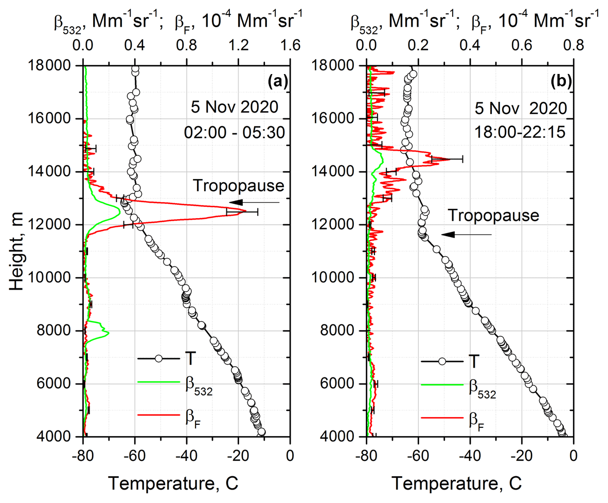
Figure 2 Vertical profiles of aerosol backscattering coefficient β₅₃₂ and fluorescence backscattering coefficient β_F on 5 November 2020 for the periods (a) 02:00–05:30 UTC and (b) 18:00–22:15 UTC. Open symbols show the temperature profile measured by the radiosonde launched at Herstmonceux (UK).

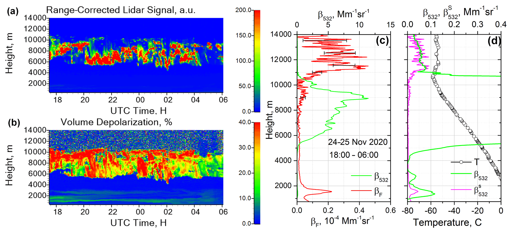
Figure 3 Smoke fluorescence in the presence of clouds on 24–25 November 2020. (a, b) Spatiotemporal variations in the range-corrected lidar signal and volume depolarization at 1064 nm. (c) Vertical profiles of the aerosol β₅₃₂ and fluorescence β_F backscattering coefficients. (d) Aerosol backscattering coefficient β₅₃₂, together with smoke backscattering coefficient ${\mathit{\beta }}_{\mathrm{532}}^{\mathrm{s}}$, computed from β_F for G_F = 4.5 × 10⁻⁴. Open symbols show temperature profile measured by the radiosonde at Herstmonceux.

3 Results of the measurements

3.1 Observation of smoke particles in UTLS

Smoke particles produced by intensive fires and transported across the Atlantic are regularly observed in the UTLS height range over Europe (Müller et al., 2005; Hu et al., 2019; Baars et al., 2019, 2021). One such event, observed over Lille in the night of 4–5 November 2020, is shown in Fig. 1. The figure provides height–time displays of the range-corrected lidar signal and the volume depolarization ratio at 1064 nm, together with the fluorescence backscattering coefficient. A narrow smoke layer occurred in the upper troposphere in the period from 23:00–06:00 UTC. The smoke was detected at heights above 12 km after midnight. The particles caused a low volume depolarization ratio (< 5 %) at 1064 nm and strong fluorescence backscattering (β_F> 1.2 × 10⁻⁴ Mm⁻¹ sr⁻¹). The backward trajectory analysis indicated that the aerosol layer was transported over the Atlantic and contained products of North American wild fires.

Vertical profiles of aerosol β₅₃₂ and fluorescence β_F backscattering coefficients for the period from 02:00–05:30 UTC are shown in Fig. 2a. The fluorescence capacity G_F in the center of smoke layer (not shown) was about 4.5 × 10⁻⁴. The depolarization ratio of aged smoke in the UTLS height range usually shows a strong spectral dependence (Haarig et al., 2018; Hu et al., 2019). For the case presented in Fig. 2a the particle depolarization ratio in the center of the smoke layer decreased from 16 ± 4 % at 355 nm (δ₃₅₅) to 4 ± 1 % at 1064 (δ₁₀₆₄). The tropopause height H_tr was at about 13 000 m; thus the main part of the smoke layer was below the tropopause. By the end of day the smoke layer became weaker (β_F < 0.3 × 10⁻⁴ Mm⁻¹ sr⁻¹) and ascended up to 14 500 m, which is above the tropopause. The corresponding vertical profiles of β₅₃₂ and β_F are shown in Fig. 2b. The fluorescence capacity in the center of the layer is about 4.5 × 10⁻⁴, which is close to the value observed during the 02:00–05:30 UTC period.

An important advantage of the fluorescence lidar technique is the ability to monitor smoke particles inside cirrus clouds. The results of smoke observations in the presence of ice clouds are shown in Fig. 3. Cirrus clouds occurred during the whole night in the height range from 6.0–10.0 km. To quantify the fluorescence backscattering inside the cloud (which was rather weak in this case), the lidar signals were averaged over the full 18:00–06:00 UTC time interval in Fig. 3a. The fluorescence backscatter coefficient shown in Fig. 3c decreased from β_F = 0.015 × 10⁻⁴ Mm⁻¹ sr⁻¹ at 5000 m (near the cloud base) to a minimum value of 0.01 × 10⁻⁴ Mm⁻¹ sr⁻¹ at 7000 m inside the cirrus layer. Above the tropopause the fluorescence backscattering increased strongly and reached the maximum (about 0.3 × 10⁻⁴ Mm⁻¹ sr⁻¹) at 11 000–13 000 m height.

Figure 4 Range-corrected lidar signal at 1064 nm on 23–24 June 2020, revealing a smoke layer between 4500 and 5200 m height.

The analysis of fluorescence measurements performed during strong smoke episodes in the summer and autumn of 2020, when smoke layers from North American fires frequently reached Europe, demonstrates that the fluorescence capacity varied within the range of 2.5 × 10⁻⁴ to 4.5 × 10⁻⁴. The variations are a function of smoke composition, relative humidity and particle size. However, in the upper troposphere where relative humidity is low, G_F was normally close to 4.5 × 10⁻⁴. This relatively low range of G_F variations allows the estimation of the backscattering coefficient attributed to the smoke particles from fluorescence measurements as follows:

$$\begin{array}{}\text{(1)}& {\mathit{\beta }}_{\mathrm{532}}^{\mathrm{s}}={\displaystyle \frac{{\mathit{\beta }}_{\mathrm{F}}}{G_{\mathrm{F}}}}.\end{array}$$

Figure 3d shows the smoke backscattering coefficient ${\mathit{\beta }}_{\mathrm{532}}^{\mathrm{s}}$, calculated from β_F for G_F = 4.5 × 10⁻⁴, together with β₅₃₂. The dynamical range of β₅₃₂ variations is high. To make smoke backscattering visible above H_tr, β₅₃₂ is plotted in expanded scale in Fig. 3d. The ${\mathit{\beta }}_{\mathrm{532}}^{\mathrm{s}}$ values, though strongly oscillating above the tropopause, match the β₅₃₂, indicating that the smoke contribution to backscattering was predominant.

3.2 Estimation of smoke particle content based on fluorescence measurements

The possibility to detect fluorescence backscattering inside the cirrus clouds reveals also the opportunity for a quantitative characterization of the smoke content. This can be realized by a synergistic use of fluorescence and multiwavelength Mie–Raman lidar observations. The flow chart, summarizing the main steps of this procedure, is presented in Appendix A. For the smoke layers with sufficient optical depth, the number N, surface area S and volume V concentrations can be evaluated by inverting the 3β+2α observations consisting of three backscatter coefficients (355, 532, 1064 nm) and two extinction coefficients (355, 532 nm) (Müller et al., 1999; Veselovskii et al., 2002; Pérez-Ramírez et al., 2013). The conversion factors C_N, C_S and C_V, introduced as

$$\begin{array}{}\text{(2)}& C_N={\displaystyle \frac{N}{{\mathit{\beta }}_{\mathrm{F}}}},C_S={\displaystyle \frac{S}{{\mathit{\beta }}_{\mathrm{F}}}},C_V={\displaystyle \frac{V}{{\mathit{\beta }}_{\mathrm{F}}}},\end{array}$$

allow the estimation of smoke particle concentration inside the clouds from fluorescence backscattering, assuming that smoke contribution to the fluorescence is predominant. Moreover, it allows the estimation of the particle concentration in weak smoke layers in UTLS, where 3β+2α observations are normally not available.

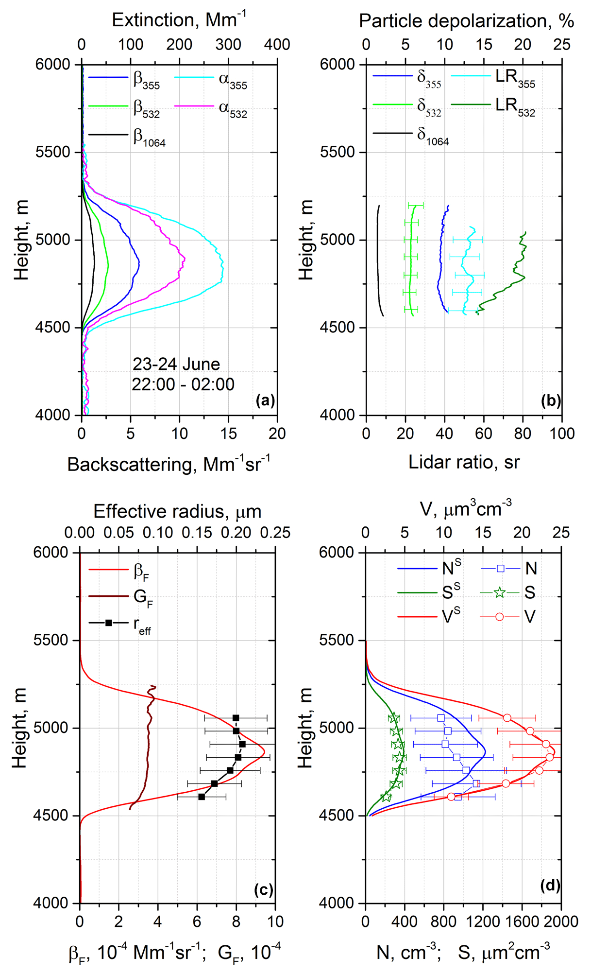
Figure 5 Smoke layer on 23–24 June 2020. (a) Vertical profiles of backscattering (β₃₅₅, β₅₃₂, β₁₀₆₄) and extinction (α₃₅₅, α₅₃₂) coefficients. (b) Particle depolarization ratios (δ₃₅₅, δ₅₃₂, δ₁₀₆₄) and lidar ratios (LR₃₅₅, LR₅₃₂). (c) Fluorescence backscattering (β_F), fluorescence capacity (G_F) and the particle effective radius (r_eff). (d) Number (N, N^S), surface area (S, S^S) and volume (V, V^S) concentrations obtained by inversion of 3β+2α observations (symbols) and calculated from the fluorescence backscattering (lines) by using the mean conversion factors defined in Eq. (2).

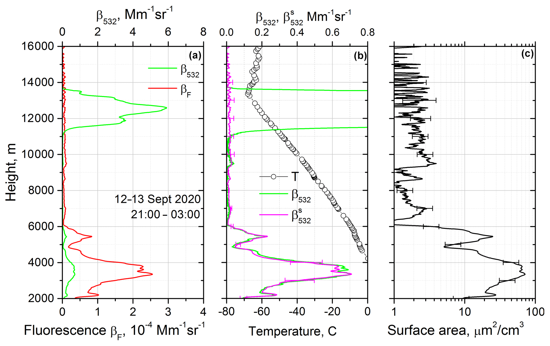
Figure 6 Observation of smoke fluorescence on 12–13 September 2020 at 21:00–03:00 UTC. (a) Vertical profiles of the aerosol backscattering coefficient β₅₃₂ and fluorescence backscattering coefficient β_F. (b) Aerosol backscattering coefficient β₅₃₂, together with smoke backscattering coefficient ${\mathit{\beta }}_{\mathrm{532}}^{\mathrm{s}}$, computed from β_F for G_F = 3.6 × 10⁻⁴. (c) Surface area concentration of the smoke particles calculated from β_F using the respective conversion factor from Eq. (3). Open symbols show the temperature profile measured by the radiosonde at Herstmonceux.

On 23–24 June 2020, a strong smoke layer was observed at 4500–5500 m height during the whole night (Fig. 4). The vertical profiles of the aerosol backscattering and extinction coefficients (3β+2α) are shown in Fig. 5a, while the particle depolarization ratios δ₃₅₅, δ₅₃₂ and δ₁₀₆₄ and the lidar ratios at 355 and 532 nm (LR₃₅₅, LR₅₃₂) are presented in Fig. 5b. The depolarization ratio decreases with wavelength from 9 ± 1.5 % at 355 nm to 1.5 ± 0.3 % at 1064 nm, and the lidar ratio at 532 nm significantly exceeds the corresponding value at 355 nm (80 ± 12 and 50 ± 7.5 sr respectively), which is typical for aged smoke (Müller et al., 2005). The multiwavelength observations were inverted to determine the particle effective radius r_eff, number, surface area and volume concentrations for seven height bins inside the smoke layer. The effective radius r_eff in Fig. 5c increases through the layer from 0.15–0.2 µm simultaneously with the increase in the fluorescence capacity G_F from 2.8 × 10⁻⁴–3.6 × 10⁻⁴. Retrieved values of N, S and V were used for the calculation of the conversion factors (Eq. 2) for each height bin. In the center of the smoke layer (at 4.9 km) the factors are C_N = 88 × 10⁴ cm⁻³ (Mm⁻¹ sr⁻¹)⁻¹, C_S = 35 × 10⁴ µm² cm⁻³ (Mm⁻¹ sr⁻¹)⁻¹ and C_V = 2.4 × 10⁴ µm³ cm⁻³ (Mm⁻¹ sr⁻¹)⁻¹ (thus, when β_F is given in Mm⁻¹ sr⁻¹, the calculated values of N, S and V are given in cm⁻³, µm²cm⁻³ and µm³cm⁻³ respectively). Fluorescence backscattering is proportional to the particle volume concentration, so C_V is not sensitive to the effective radius variation. The conversion factors C_N and C_S, on the contrary, depend on the particle size. Figure 5d shows the profiles of N, S and V obtained by the inversion of 3β+2α observations (symbols), together with corresponding values (N^S, S^S, V^S) obtained from β_F, using the mean conversion factors for the seven height bins considered. The volume concentrations V and V^S agree well for all seven height bins. For the surface area concentrations the agreement is still good, but for N and N^S the difference is up to 30 %. We need to emphasize that the conversion factors presented are specific for our lidar system (for the interference filter installed in the fluorescence channel). It is worthwhile to mention that the ratio $V/{\mathit{\alpha }}_{\mathrm{532}}$ of the volume concentration V in Fig. 5d to the extinction coefficient α at 532 nm in Fig. 5a, as well as the ratio $S/{\mathit{\alpha }}_{\mathrm{532}}$, is very close to respective extinction-to-volume and extinction-to-surface-area-concentration conversion factors presented for aged wildfire smoke by Ansmann et al. (2021).

Table 1 Conversion factors C_N, C_S and C_V and fluorescence capacity G_F at height H for five smoke episodes. Volume and surface area concentrations of smoke particles, obtained by the inversion of β+2α lidar observations (V, S), are given, together with values calculated from fluorescence measurements (V^S, S^S) and using conversion factors (Eq. 3).

Figure 7 Formation of ice particles at heights above 10 km inside a smoke layer on 11–12 September 2020. Spatiotemporal variations in range-corrected lidar signal at 1064 nm, volume depolarization ratio at 1064 nm and fluorescence backscattering coefficient (in 10⁻⁴ Mm⁻¹ sr⁻¹).

The conversion factors depend on the smoke composition. To estimate the variation range of C_N, C_S and C_V, several smoke episodes were analyzed, and corresponding results are presented in Table 1. The table provides the fluorescence capacity G_F and the conversion factors at the heights where 3β+2α data could be calculated. Mean values of 〈C_N〉, 〈C_S〉 and 〈C_V〉 derived for these episodes and corresponding standard deviations are

$$\begin{array}{}\text{(3)}& \begin{array}{rl}& \langle C_N\rangle =(\mathrm{61}\pm \mathrm{32})\times {\mathrm{10}}^{\mathrm{4}}{\mathrm{cm}}^{-\mathrm{3}}({\mathrm{Mm}}^{-\mathrm{1}}{\mathrm{sr}}^{-\mathrm{1}}{)}^{-\mathrm{1}},\\ & \langle C_S\rangle =(\mathrm{28}\pm \mathrm{6.4})\times {\mathrm{10}}^{\mathrm{4}}\mathrm{\mu }{\mathrm{m}}^{\mathrm{2}}{\mathrm{cm}}^{-\mathrm{3}}({\mathrm{Mm}}^{-\mathrm{1}}{\mathrm{sr}}^{-\mathrm{1}}{)}^{-\mathrm{1}},\\ & \langle C_V\rangle =(\mathrm{2.2}\pm \mathrm{0.2})\times {\mathrm{10}}^{\mathrm{4}}\mathrm{\mu }{\mathrm{m}}^{\mathrm{3}}{\mathrm{cm}}^{-\mathrm{3}}({\mathrm{Mm}}^{-\mathrm{1}}{\mathrm{sr}}^{-\mathrm{1}}{)}^{-\mathrm{1}}.\end{array}\end{array}$$

Table 1 shows also the volume and surface area concentrations of the smoke particles obtained from the inversion of 3β+2α observations (V, S) and calculated from β_F (V^S, S^S) using the conversion factors in Eq. (3). Standard deviations of V^S and S^S from corresponding values of V_3β+2α and S_3β+2α are 10 % and 25 % respectively.

Table 2 Number N^S, surface area S^S and volume V^S concentrations of smoke particles inside the ice cloud at height H estimated from fluorescence measurements by applying the conversion factors in Eq. (3) for four measurement sessions.

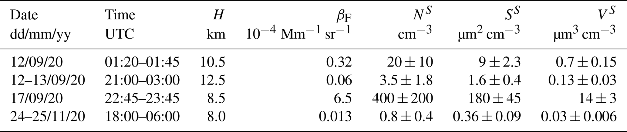
The mean conversion factors in Eq. (3) are now used to estimate the smoke microphysical properties inside the cloud, assuming in addition that the predominant contribution to the fluorescence is provided by the smoke. Table 2 summarizes the number, surface area and volume concentrations of smoke particles inside the ice clouds, estimated from fluorescence measurements for four episodes considered in this paper. On 12–13 September 2020, the smoke layer with high fluorescence and low depolarization ratio at 1064 nm (below 4 %) was observed during the whole night inside the 2.0–5.0 km height range. The cirrus cloud occurred above 11 000 m also during the whole night. Figure 6a presents vertical profiles of the aerosol β₅₃₂ and fluorescence β_F backscattering coefficients. Fluorescence backscattering shows a maximum at 3.5 km, but it is detected even inside the cloud. The smoke backscattering coefficient ${\mathit{\beta }}_{\mathrm{532}}^{\mathrm{s}}$, computed from β_F for G_F = 3.6 × 10⁻⁴, agrees well with β₅₃₂ inside the 2.0–10.0 km height range (Fig. 6b). The height profile of the surface area concentration of the smoke particle S^S, calculated from β_F using the respective conversion factor in Eq. (3), is shown in Fig. 6c. In the smoke layer, S^S is up to 60 µm² cm⁻³, while in the center of the cloud at 12–13 km height the average value of S^S is 1.6 ± 0.4 µm² cm⁻³. Corresponding values of number and volume concentrations in the cloud center are 3.5 ± 1.8 cm⁻³ and 0.13 ± 0.013 µm³ cm⁻³.

The temperature in the cloud ranged from about −50 to almost −70 ^∘C and was −68 ^∘C at cirrus top in Fig. 6b where ice nucleation usually starts. We applied the immersion freezing INP parameterization of Knopf and Alpert (2013) for leonardite (a standard humic acid surrogate material) and assume that this humic compound represents the amorphous organic coating of smoke particles. The INP parameterization for smoke particles is summarized for lidar applications in Ansmann et al. (2021). The selected parameterization allows the estimation of the INP concentration as a function of ambient air temperature (freezing temperature), ice supersaturation, particle surface area and time period for which a certain level of ice supersaturation is given. We simply assume a constant ice supersaturation of around 1.45 during a time period of 600 s (upwind phase of a typical gravity wave in the upper troposphere). The temperature at cirrus top height is set to −68 ^∘C and the aerosol surface area concentration to 2.0 µm² cm⁻³ as indicated in Fig. 6c. The obtained INP concentrations of 1–10 L⁻¹ for these meteorological and aerosol environmental conditions can be regarded as the predicted number concentration of ice crystals nucleated in the cirrus top region. Ice crystal number concentrations of 1–10 L⁻¹ are typical values in cirrus layers when heterogeneous ice nucleation dominates (typical values of INP concentrations and supersaturation are discussed, for example, in Sullivan et al., 2016; Ansmann et al., 2019b, 2021; Engelmann et al., 2021). It should be mentioned that the required very high ice supersaturation levels of close to 1.5 (ice supersaturation of 1.1–1.2 is sufficient in the case of mineral dust particles) are still lower than the threshold supersaturation level of > 1.5 at which homogeneous freezing starts to dominate. At low updraft velocities around 10–25 cm s⁻¹, as usually given in gravity waves in the upper troposphere (Barahona et al., 2017), heterogeneous ice nucleation very likely dominates the ice production when cirrus evolves in detected aerosol layers.

3.3 Ice formation inside the smoke layers

During September 2020 we observed several episodes with ice cloud formation inside of smoke layers. One such episode occurred on 11–12 September 2020 and is shown in Fig. 7. The height–time display of the fluorescence backscattering coefficient reveals the smoke layer in the 5.0–10.0 km height range. Inside this layer, we can observe a short time interval of 15 min with a strongly increased depolarization ratio around 10.5 km height (red spots), indicating ice cloud formation. Figure 8 shows vertical profiles of the aerosol backscattering coefficients β₃₅₅, β₅₃₂ and β₁₀₆₄, as well the particle depolarization ratios δ₃₅₅, δ₅₃₂ and δ₁₀₆₄, for two temporal intervals. The first interval (23:00–00:30 UTC) is prior to ice cloud formation, and the second one (01:20–01:45 UTC) covers the ice occurrence period. The depolarization ratios at all three wavelengths were < 5 % below 6 km height. Above that height δ₃₅₅ significantly increased reaching the value of 10 % at 7 km (Fig. 8b), which is indicative of a change in the particle shape (from spherical to irregular shape). The fluorescence capacity also changed with height, being about G_F = 4.5 × 10⁻⁴ at 5.5 km, and it decreases to 3.5 × 10⁻⁴ by 8 km. The profile of ${\mathit{\beta }}_{\mathrm{532}}^{\mathrm{s}}$ shown in Fig. 8c is calculated assuming G_F = 4.0 × 10⁻⁴, and it matches well the profile of β₅₃₂ for the whole height range. The aerosol layer at 10.5 km is thus a pure smoke layer. Ice formation at 10.5 km (Fig. 8d–f) leads to a significant increase in β₅₃₂, while ${\mathit{\beta }}_{\mathrm{532}}^{\mathrm{s}}$ (or the respective fluorescence backscatter coefficient β_F) remains low and at the same level as observed below the cirrus layer, i.e., below 10 km height. The depolarization ratios at all three wavelengths increases to typical cirrus values around 40 %. The temperature at 10.5 km is about −50 ^∘C, and the surface area concentration of the smoke particles inside the cloud, estimated from β_F, is about 10 µm² cm⁻³ (see Fig. 8f, thin blue line). For these temperature and aerosol conditions, smoke INP concentrations of 1–10 L⁻¹ are yielded for ice supersaturation values even below 1.4 (1.38–1.4) and updraft duration of 600 s. When comparing Fig. 8c and f at cirrus level it seems to be that ice nucleation on the smoke particles widely depleted the smoke INP reservoir.

Figure 8 Formation of ice particles at 10–11 km height inside a smoke layer on 11–12 September 2020. Vertical profiles of (a, d) the aerosol backscattering coefficients β₃₅₅, β₅₃₂ and β₁₀₆₄; (b, e) the particle depolarization ratios δ₃₅₅, δ₅₃₂ and δ₁₀₆₄; and (c, f) β₅₃₂, together with backscattering coefficient of smoke ${\mathit{\beta }}_{\mathrm{532}}^{\mathrm{s}}$, calculated from fluorescence backscattering β_F assuming G_F = 4.0 × 10⁻⁴. Panel (f) shows also the smoke surface area concentration S^S of the smoke particles calculated from β_F by applying the respective conversion factor in Eq. (3). Results are given for the time intervals 23:00–00:30 and 01:20–01:45 UTC, which are prior to and during ice cloud formation at 10.5 km height. The temperature profile measured by the radiosonde at Herstmonceux is shown with open symbols in panel (c).

Figure 9 Formation of ice particles at heights above 8 km inside the smoke layer on 17–18 September 2020. Spatiotemporal variations in range-corrected lidar signal at 1064 nm, volume depolarization ratio at 1064 nm and fluorescence backscattering coefficient (in 10⁻⁴ Mm⁻¹ sr⁻¹).

Another case of ice formation in the smoke layer was observed on 17–18 September 2020. Strong smoke layers occurred in the 5.0–9.0 km height range as shown in Fig. 9. During the period from 22:30–00:00 UTC, the depolarization increased at 8.5 km height, indicating ice formation. Vertical profiles of the particle parameters prior to and during ice formation are shown in Fig. 10. The ${\mathit{\beta }}_{\mathrm{532}}^{\mathrm{s}}$ calculated for G_F = 3.5 × 10⁻⁴ matches well with β₅₃₂ below 6.9 km and above 8.0 km (Fig. 10c), but inside the 7.0–8.0 km height range ${\mathit{\beta }}_{\mathrm{532}}>{\mathit{\beta }}_{\mathrm{532}}^{\mathrm{s}}$, meaning that G_F was decreased. The depolarization ratio in the 7.0–8.0 km height range shows some enhancement (Fig. 10b): in particular, δ₅₃₂ increased from 10 %–12 %. Cloud formation at 8.5 km (Fig. 10d) led to a significantly smaller increase in the depolarization ratio compared to the case on 11–12 September. Prior to the cloud formation the values of δ₁₀₆₄, δ₅₃₂ and δ₃₅₅ at 8.5 km were 3 %, 10 % and 13 % respectively (Fig. 10b), and in the cloud corresponding depolarization ratios increase up to 9 %, 15 % and 20 %. The reason is probably that the signal averaging period from 22:45–23:45 UTC includes a cloud-free section. Three gravity waves obviously crossed the lidar field site and triggered ice nucleation just before 23:00 UTC, 15–30 min after 23:00 UTC and around midnight (00:00 UTC). The temperature at cloud top at about 8.5–8.6 km height was close to −35 ^∘C. For this high temperature and the high particle surface area concentration of 200 µm² cm⁻³ (see Fig. 10d, thin blue line), smoke INP concentrations of 1–10 L⁻¹ are yielded for a relatively low ice supersaturation of 1.30–1.33 and an updraft period of 600 s. Again, a depletion of the INP reservoir is visible after the formation of the cirrus layer (see Fig. 6c and d around and above 8.5 km height).

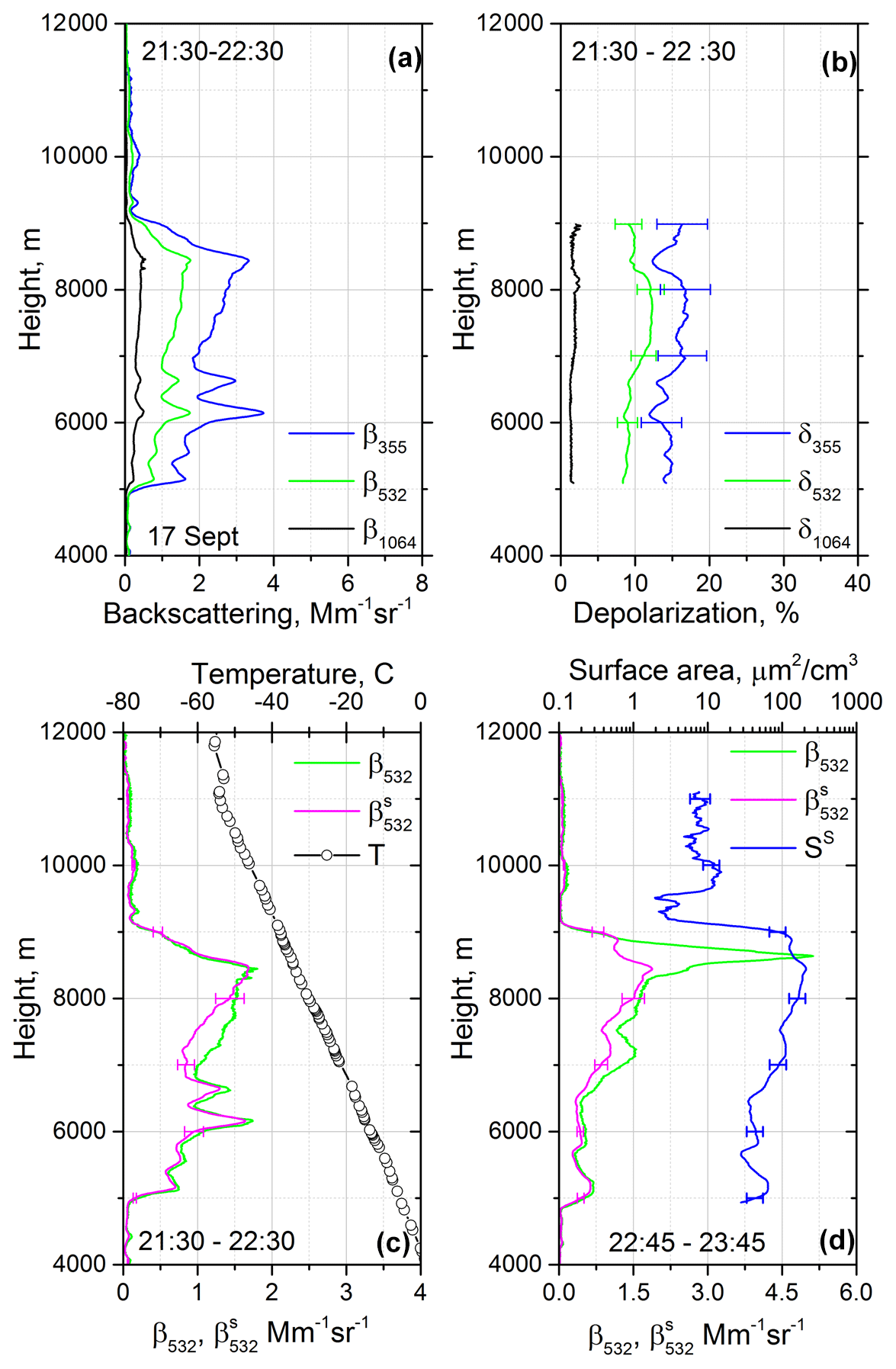
Figure 10 Formation of ice particles at 8.5–8.6 km height inside a smoke layer on 17 September 2020. Vertical profiles of (a) the aerosol backscattering coefficients β₃₅₅, β₅₃₂ and β₁₀₆₄; (b) the particle depolarization ratios δ₃₅₅, δ₅₃₂ and δ₁₀₆₄; and (c, d) β₅₃₂, together with backscattering coefficient of smoke ${\mathit{\beta }}_{\mathrm{532}}^{\mathrm{s}}$, calculated from fluorescence backscattering β_F assuming G_F = 3.5 × 10⁻⁴. Results are given for the time intervals (a–c) 21:30–22:30 UTC and (d) 22:45–23:45 UTC, which are prior to and during ice formation at 8.5 km height. Panel (d) shows also the surface area concentration of the smoke particle S^S calculated from β_F by applying the respective conversion factor from Eq. (3). The temperature profile measured by the radiosonde at Herstmonceux is shown with open symbols in panel (c).

4 Conclusion

The operation of a fluorescence channel in the LILAS lidar during strong smoke events in the summer and autumn seasons of 2020 has demonstrated the ability of the fluorescence lidar technique to discriminate ice from smoke particles in atmospheric layers in the UTLS height range in great detail. The fluorescence capacity G_F of smoke particles during this period varied within a relatively small range: 2.5–4.5 × 10⁻⁴; thus the use of the mean value of G_F allows us to estimate the contribution of smoke to the total particle backscattering coefficient. The fluorescence lidar technique makes it possible to estimate smoke parameters, such as number, surface area and volume concentration, in the UTLS height range in a quantitative way by applying conversion factors (C_N, C_S, C_V) which link the fluorescence backscattering and the smoke microphysical properties. These factors, derived from the synergy of multiwavelength Mie–Raman and fluorescence lidar observations, show some variation from episode to episode; however, the use of mean values 〈C_N〉, 〈C_S〉 and 〈C_V〉 allows the estimation of smoke properties in the UTLS height regime with reasonable accuracy. Based on two case studies, we demonstrated that the fluorescence lidar technique provides the unique possibility to characterize the smoke particles and their amount inside cirrus cloud layers. The smoke input parameter (surface area concentration) in smoke INP parameterization schemes that are used to predict ice crystal number concentrations in cirrus generation cells can now be estimated within freshly formed cirrus layers.

The smoke parameters such as fluorescence capacity and conversion factors were derived from observations of aged wildfire smoke transported over the Atlantic in 2020. However, smoke composition depends on many factors, such as burning materials type, flame temperature and environmental conditions; thus the smoke fluorescence properties may also vary. Hence, it is important to perform the measurements for different locations and seasons. The fluorescence backscattering in the UTLS height range is quite weak, so to perform measurements with higher temporal resolution, more powerful lidar systems are needed. A dedicated high-power lidar, LIFE (laser induced fluorescence explorer), will be designed and operated at ATOLL in the frame of OBS4CLIM/ACTRIS-France.

Appendix A: Estimation of smoke parameters from Mie–Raman and fluorescence lidar measurements

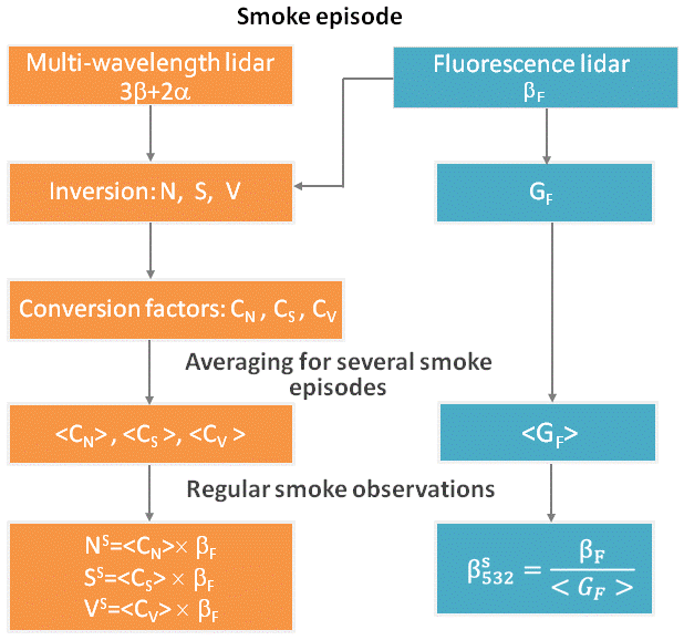
Figure A1 Flow chart showing the main steps of the procedure of smoke parameter estimation from multiwavelength Mie–Raman and fluorescence lidar measurements. Procedure includes the following steps. (i) For a strong smoke layer the 3β+2α data set, derived from multiwavelength Mie–Raman lidar observations, is inverted to the particle number N, surface S and volume V density. (ii) Conversion factors C_N, C_S and C_V are calculated from Eq. (2) by using the fluorescence backscattering coefficient β_F. (iii) Different smoke events are analyzed to get mean values of conversion factors 〈C_N〉, 〈C_S〉 and 〈C_V〉. These mean values are used to estimate smoke concentration in weak layers in UTLS and inside cirrus clouds in regular observations. The mean value of smoke fluorescence capacity 〈G_F〉 allows the estimation of smoke contribution ${\mathit{\beta }}_{\mathrm{532}}^{\mathrm{s}}$ to the total backscattering coefficient β₅₃₂.