Aerosol optical properties calculated from size distributions, filter samples and absorption photometer data at Dome C, Antarctica, and their relationships with seasonal cycles of sources

Optical properties of surface aerosols at Dome C, Antarctica, in 2007–2013 and their potential source areas are presented. Scattering coefficients (σ_sp) were calculated from measured particle number size distributions with a Mie code and from filter samples using mass scattering efficiencies. Absorption coefficients (σ_ap) were determined with a three-wavelength Particle Soot Absorption Photometer (PSAP) and corrected for scattering by using two different algorithms. The scattering coefficients were also compared with σ_sp measured with a nephelometer at the South Pole Station (SPO). The minimum σ_ap was observed in the austral autumn and the maximum in the austral spring, similar to other Antarctic sites. The darkest aerosol, i.e., the lowest single-scattering albedo ω_o≈0.91, was observed in September and October and the highest ω_o≈0.99 in February and March. The uncertainty of the absorption Ångström exponent α_ap is high. The lowest α_ap monthly medians were observed in March and the highest in August–October. The equivalent black carbon (eBC) mass concentrations were compared with eBC measured at three other Antarctic sites: the SPO and two coastal sites, Neumayer and Syowa. The maximum monthly median eBC concentrations are almost the same ($\sim \mathrm{3}\pm \mathrm{1}$ ng m⁻³) at all these sites in October–November. This suggests that there is no significant difference in eBC concentrations between the coastal and plateau sites. The seasonal cycle of the eBC mass fraction exhibits a minimum f(eBC) ≈0.1 % in February–March and a maximum ∼4 %–5 % in August–October. Source areas were calculated using 50 d FLEXPART footprints. The highest eBC concentrations and the lowest ω_o were associated with air masses coming from South America, Australia and Africa. Vertical simulations that take BC particle removal processes into account show that there would be essentially no BC particles arriving at Dome C from north of latitude 10^∘ S at altitudes <1600 m. The main biomass-burning regions Africa, Australia and Brazil are more to the south, and their smoke plumes have been observed at higher altitudes than that, so they can get transported to Antarctica. The seasonal cycle of BC emissions from wildfires and agricultural burning and other fires in South America, Africa and Australia was calculated from data downloaded from the Global Fire Emissions Database (GFED). The maximum total emissions were in August–September, but the peak of monthly average eBC concentrations is observed 2–3 months later in November, not only at Dome C, but also at the SPO and the coastal stations. The air-mass residence-time-weighted BC emissions from South America are approximately an order of magnitude larger than from Africa and Oceania, suggesting that South American BC emissions are the largest contributors to eBC at Dome C. At Dome C the maximum and minimum scattering coefficients were observed in austral summer and winter, respectively. At the SPO σ_sp was similar to that observed at Dome C in the austral summer, but there was a large difference in winter, suggesting that in winter the SPO is more influenced by sea-spray emissions than Dome C. The seasonal cycles of σ_sp at Dome C and at the SPO were compared with the seasonal cycles of secondary and primary marine aerosol emissions. The σ_sp measured at the SPO correlated much better with the sea-spray aerosol emission fluxes in the Southern Ocean than σ_sp at Dome C. The seasonal cycles of biogenic secondary aerosols were estimated from monthly average phytoplankton biomass concentrations obtained from the Cloud-Aerosol Lidar with Orthogonal Polarization (CALIOP) satellite sensor data. The analysis suggests that a large fraction of the biogenic scattering aerosol observed at Dome C has been formed in the polar zone, but it may take a month for the aerosol to be formed, be grown and get transported from the sea level to Dome C.

1 Introduction

The Antarctic interior region has scarce observations of atmospheric constituents, and many aspects of the atmospheric properties are underdetermined. The Antarctic dome or the polar vortex, which is much stronger than its northern counterpart and present throughout the year (Karpetchko et al., 2005), at most times efficiently prevents transport into the Antarctic troposphere from lower latitudes. However, wildfires and agricultural burning emissions from Africa, South America and Australia do affect vast regions of the Southern Hemisphere, including Antarctica. For instance, Hara et al. (2010) found that haze episodes at Syowa Station, during which visibility can drop to 10 km for periods of ∼30 h, were caused by biomass-burning aerosol from South America transported to the Antarctic coast via the eastward approach of cyclones. At the Neumayer station large-scale meridional transport of biomass-burning-derived black carbon, preferentially from South America, seems to determine the BC burden and causes a distinct and consistent spring/early summer concentration maximum (Weller et al., 2013).

Concordia Station lies on Dome C (75^∘06^′ S, 123^∘23^′ E) at 3233 m a.s.l. (above sea level) on the East Antarctic Plateau, about 1100 km from the nearest coastline, the Ross Sea. The base is French and Italian operated, with research fields within astronomy and glaciology as well as atmospheric sciences. The atmospheric instrumentation is located in a small cabin southwest of the main base (at the site described by Udisti et al., 2012), where it is upwind of the base at the prevailing wind directions. Concordia is one of only three permanent year-round stations operated on the Antarctic Plateau, the others being the American Amundsen–Scott Observatory (South Pole Station (SPO), 2835 m a.s.l., about 1300 km from the nearest open sea, 1600 km away from Dome C) and the Russian Vostok station (78^∘28^′ S, 106^∘51^′ E, 3488 m.a.s.l., 600 km away). Thus, there are large spatial distances between the continuous atmospheric observations. However, properties of the Antarctic atmosphere tend to extend over both longer temporal and spatial scales than elsewhere (Fiebig et al., 2014), suggesting that the scarce observations that exist can be assumed to be representative of larger areas than is typical in other climate regions. This would imply that Dome C is an important indicator for the entire Antarctic inland. Though measurement conditions are harsh, the continuous long-term monitoring provided here can be a baseline for the aerosol optical properties of the Antarctic inland and may provide indications of changes in atmospheric constituents and aerosol levels.

There are several studies on the aerosol chemical composition at Dome C (e.g., Jourdain et al., 2008; Becagli et al., 2012, 2021; Udisti et al., 2004, 2012; Legrand et al., 2016, 2017a, b), and the aerosol optical depth (AOD) has also been measured there (Tomasi et al., 2007). However, in situ surface aerosol scattering and absorption coefficients at Dome C have not been presented. The light absorption coefficient and particle number size distributions (PNSDs) have been measured continuously with a three-wavelength Particle Soot Absorption Photometer (PSAP) and a differential mobility particle sizer (DMPS) since 2007. The PNSD data have already been used in several papers. Järvinen et al. (2013) analyzed the seasonal cycle and modal structure of PNSDs measured with the DMPS, Chen et al. (2017) analyzed the number size distribution of air ions measured with an air ion spectrometer (AIS) and the PNSD measured with the DMPS, and Lachlan-Cope et al. (2020) used the Dome C DMPS data for comparing with the PNSD measured at the coastal site Halley. The PSAP data, however, have not been presented in detail. Caiazzo et al. (2021) used some of the PSAP data mainly for evaluating elemental carbon (EC) sample contamination. Grythe (2017) used the data from 2007 to 2013 as part of his PhD thesis, but in the present paper we will analyze that period in more detail. Here we will describe the methods for measuring absorption and calculating scattering from the size distributions and filter samples.

The goals of the paper are to present descriptive statistics of extensive and intensive aerosol optical properties at Dome C in 2007–2013, their seasonal cycles, and the relationships between the seasonal cycles of major sources of absorbing and scattering aerosols. The aerosol optical properties (AOPs) will be compared with other observations from other Antarctic sites, in most detail the scattering coefficients measured at the South Pole.

2 Methods

2.1 Sampling site

Concordia Station is a permanently operated French and Italian Antarctic research base on the East Antarctic Plateau. The observations are performed at isolated sites around the main base. The Dome C sampling site is the same as used by Udisti et al. (2012), Becagli et al. (2012), and Järvinen et al. (2013). It is located about 1 km southwest of the station's main buildings, upwind in the direction of the prevailing wind. The northeastern direction (10–90^∘) has been declared the contaminated sector. Below the validity of the contaminated sector will be analyzed by using the absorption photometer data. For in situ aerosol instrumentation the sample air was taken at the flow rate of 5 L min⁻¹ from the roof of the cabin with a straight 2 m-long 25 mm diameter stainless steel tube inlet. It was covered with a protective cap to protect against snowfall and ice buildup.

2.2 Instruments

2.2.1 Aerosol measurements

Light absorption by particles was measured with a Radiance Research 3λ PSAP at three wavelengths, λ=467, 530, and 660 nm. There was no nephelometer measuring scattering coefficient, so it was calculated from particle size distributions and filter sample data as described below. Particle number size distributions were measured at 10 min time resolution in the size range 10–620 nm with a custom-built differential mobility particle sizer (DMPS) as described by Järvinen et al. (2013) and in the size range 0.3–20 µm with a Grimm model 1.108 optical particle counter (OPC) in 2007–2009. RH was not measured in the Dome C sample air, but it can be safely claimed that it was dry. The absolute humidity in the air on the upper plateau is very low, and temperature varies from colder than about −20 ^∘C in the austral summer down to about 80 ^∘C in the austral winter. When air is sampled to the instruments in the measurement containers where temperature is $>+\mathrm{10}$ ^∘C, RH decreases to very low values. In addition to the in situ instruments, PM₁ and PM₁₀ filter samples were collected for chemical analyses by ion chromatography. The length of the sampling period of the PM₁ and PM₁₀ samples was 3 or 4 and 1 d, respectively.

Figure 1 The periods of the PSAP, the DMPS, the Grimm OPC and the PM₁ and PM₁₀ filter sample data. The number of hours of accepted data and the number of samples are shown in parentheses for the continuous instruments and the filter samplers, respectively.

The data coverage for the PSAP, the DMPS, the OPC, and the PM₁ and PM₁₀ filter sample data are presented in Fig. 1. The number of hours of accepted data and the number of samples are shown in parentheses for the continuous instruments and the filter samplers, respectively. The filtering criteria will be presented below (Sect. 2.4).

2.2.2 Meteorological measurements

Ambient air temperature (t), relative humidity (RH), wind speed (WS) and wind direction (WD) data were from the routine meteorological observation at the Concordia Station as part of the IPEV/PNRA project – a collaborative project between Programma Nazionale di Ricerche in Antartide (PNRA) and Institut Polaire Français Paul-Emile Victor (IPEV) (https://www.climantartide.it/, last access: 10 April 2022).

2.3 Data processing

2.3.1 Mass concentrations from size distributions

Sixty-minute average size distributions n(D_p) were first calculated from the original 10 min data and corrected for standard temperature and pressure (STP) (p=1013 hPa, T=273.15 K). The DMPS n(D_p) data were corrected for diffusion losses during the inversion (Järvinen et al., 2013; Chen et al., 2017). Mass concentrations were calculated from the number size distributions measured with the DMPS from

$$\begin{array}{}\text{(1)}& m\left(\text{DMPS}\right)={\mathit{\rho }}_{\text{p}}V\left(\text{DMPS}\right)={\mathit{\rho }}_{\text{p}}\underset{\mathrm{10}\text{nm}}{\overset{\mathrm{620}\text{nm}}{\int }}{\displaystyle \frac{\mathit{\pi }}{\mathrm{6}}}{D}_{\text{p}}^{\mathrm{3}}n\left(D_{\text{p}}\right)\text{d}{D}_{\text{p}},\end{array}$$

where the density ρ_p=1.7 g cm⁻³ was used. For a particle density of 1.7 g cm⁻³, the particle diameter 620 nm corresponds to the aerodynamic diameter $D_{\text{a}}=\sqrt{{\mathit{\rho }}_{\text{p}}/{\mathit{\rho }}_{\mathrm{0}}}{D}_{\text{p}}=\sqrt{\mathrm{1.7}}\times \mathrm{620}$ nm ≈808 nm, where ρ₀=1 g cm⁻³. To be consistent with the definitions of filter-sample size ranges that typically show the upper aerodynamic diameter of a sampler inlet, the mass concentration calculated from Eq. (1) will be referred to as m(DMPS,PM_0.8) and the volume concentration as V(DMPS,PM_0.8).

In December 2007–July 2009 particles were also measured with the Grimm 1.108 OPC that measures number concentrations of particles in the D_p range of 0.3–20 µm. The particle number concentrations in the size range D_p>1 µm were first corrected for WS-dependent and particle-diameter-dependent inlet and sampling tube losses by dividing the raw, non-corrected number concentrations n(D_p, OPC, non-corrected) with the combined inlet and tube transmittance f_inlet,tubing (WS, D_p), as described in the Supplement. The number concentrations were very small in the size ranges where the transmittance losses were significant. In a large fraction of data n(D_p, OPC, non-corrected) was zero in the particle size range where f_inlet,tubing is small. If the true concentration was larger than zero but the raw concentration in the OPC data was zero due to the instrument sensitivity and sampling losses, then the corrected concentration would also be zero even if the raw concentration was multiplied by a very large number $\mathrm{1}/f_{\text{inlet,tubing}}$. Consequently, the number concentrations and the derived mass concentrations and scattering coefficients in the large-particle size range would be underestimated. The underestimation could in principle be estimated by using a collocated more sensitive instrument sampling air through a well-defined inlet with minimal particle losses. These were not available, so a detailed analysis of the underestimations of the derived quantities was omitted from the paper.

The three largest channels of the OPC measure the number concentrations in the D_p range of 7.5–20 µm. For an assumed density ρ_p=1.7 g cm⁻³ the diameter D_p=7.5 µm corresponds to the aerodynamic diameter D_a=9.8 µm. Assuming that ρ_p is constant over the whole size range, the mass concentration of particles smaller than D_a=10 µm is calculated from the number size distributions by excluding the three largest particle OPC channels as

$$\begin{array}{}\text{(2)}& \begin{array}{rl}& m\left(n\left(D_{\text{p}}\right),{\mathrm{PM}}_{\mathrm{10}}\right)={\mathit{\rho }}_{\text{p}}V\left(n\left(D_{\text{p}}\right),{\mathrm{PM}}_{\mathrm{10}}\right)\\ & ={\mathit{\rho }}_{\text{p}}\left(V\left({\text{DMPS,PM}}_{\mathrm{0.8}}\right)+V\left({\text{OPC,PM}}_{\mathrm{0.8}-\mathrm{10}}\right).\right)\end{array}\end{array}$$

The fraction of volume concentration measured by the DMPS equals

$$\begin{array}{}\text{(3)}& fV\left(\text{DMPS}\right)={\displaystyle \frac{V\left({\text{DMPS,PM}}_{\mathrm{0.8}}\right)}{V\left(n\left(D_{\text{p}}\right),{\mathrm{PM}}_{\mathrm{10}}\right)}}.\end{array}$$

This fraction was calculated from data collected during the simultaneous operation of the DMPS and the OPC. The monthly average fV(DMPS) values presented in Table 1 were used for the period 2008–2013 to calculate mass concentrations in the size range D_a<10 µm from

$$\begin{array}{}\text{(4)}& \begin{array}{rl}& m\left({\text{DMPS,PM}}_{\mathrm{10}}\right)={\displaystyle \frac{{\mathit{\rho }}_{\text{p}}V\left({\text{DMPS,PM}}_{\mathrm{0.8}}\right)}{fV\left(\text{DMPS}\right)}}\\ & ={\displaystyle \frac{m\left({\text{DMPS,PM}}_{\mathrm{0.8}}\right)}{fV\left(\text{DMPS}\right)}}.\end{array}\end{array}$$

In other words, the variable names m(DMPS,PM_0.8) and m(DMPS,PM₁₀) will be used below to emphasize that these mass concentrations were calculated from DMPS data. The mass concentrations m(DMPS,PM_0.8) and m(DMPS,PM₁₀) can be considered to be the lower and upper estimates of m.

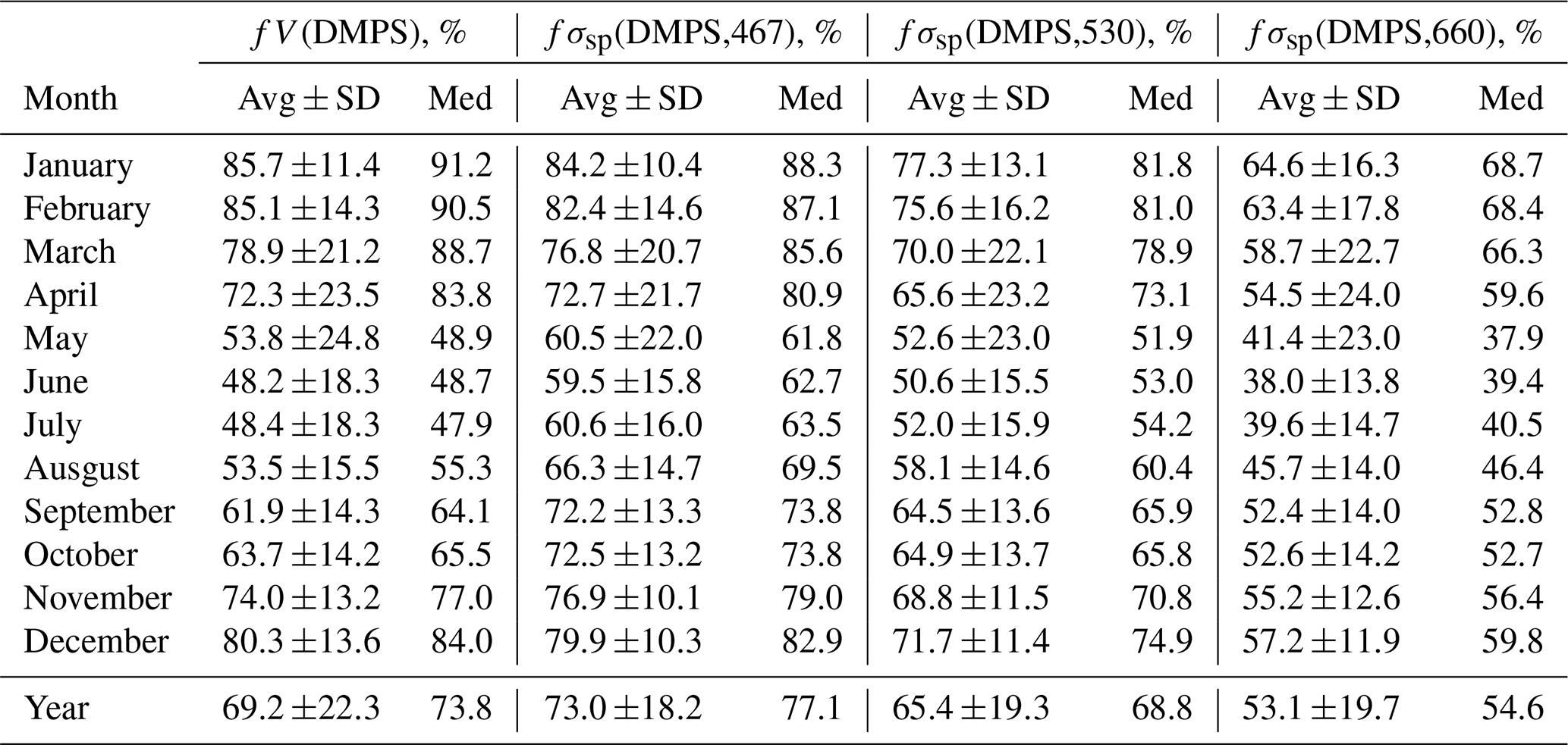
Table 1 Seasonal variation of the fractions of volume concentration fV(DMPS) (Eq. 3 in the text) and scattering coefficients fσ_sp(DMPS) (Eq. 7 in the text) at wavelengths of 467, 530, and 660 nm in the size range measured by the DMPS of the respective values calculated from the combined size distributions measured with the DMPS and the OPC at Dome C in December 2007–July 2009. Avg ± SD: average ± standard deviation; med: median.

2.3.2 Scattering coefficients from the size distributions

Scattering coefficients were calculated using the 60 min average size distributions from

$$\begin{array}{}\text{(5)}& {\mathit{\sigma }}_{\text{sp}}(m,\mathit{\lambda })=\int Q_{\text{s}}(D_{\text{p}},m,\mathit{\lambda }){\displaystyle \frac{\mathit{\pi }}{\mathrm{4}}}{D}_{\text{p}}^{\mathrm{2}}n\left(D_{\text{p}}\right)\text{d}{D}_{\text{p}},\end{array}$$

where Q_s is the scattering efficiency calculated using the Mie code by Barber and Hill (1990), m is the refractive index, λ is the wavelength, and n(D_p) is the particle number size distribution. Analogously to the mass concentrations, the scattering coefficients were determined from the simultaneous DMPS and OPC measurements in December 2007–July 2009 from

$$\begin{array}{}\text{(6)}& \begin{array}{rl}& {\mathit{\sigma }}_{\text{sp}}\left(n\left(D_{\text{p}}\right),{\mathrm{PM}}_{\mathrm{10}}\right)={\mathit{\sigma }}_{\text{sp}}\left({\text{DMPS,PM}}_{\mathrm{0.8}}\right)\\ & +{\mathit{\sigma }}_{\text{sp}}\left({\text{OPC,PM}}_{\mathrm{0.8}-\mathrm{10}}\right),\end{array}\end{array}$$

where σ_sp(OPC,PM_0.8) and σ_sp(OPC,PM_0.8−10) are the scattering coefficient calculated from the particle number size distributions in the size ranges measured by the DMPS and the OPC, respectively. As explained above, the number size distributions for D_p>1 µm were corrected for the inlet and sampling tube losses. For σ_sp(DMPS,PM_0.8) the refractive index of sulfuric acid (SA, H₂SO₄, $m_{\text{r}}=\mathrm{1.426}+\mathrm{0}i$, Seinfeld and Pandis, 2006) was used. This refractive index is slightly lower than that estimated for submicron aerosols at two low-altitude Antarctic stations, Aboa and Neumayer in Queen Maud Land. Virkkula et al. (2006) measured particle number size distributions in the size range D_p<800 nm with a DMPS and light scattering of submicron particles with a nephelometer at the Finnish site about 130 km inland from the open Weddell Sea in January 2000. With an iteration procedure matching nephelometer-measured and size-distribution-derived scattering coefficients, the real refractive indices were 1.43±0.07 and 1.45±0.04 at λ=550 nm for all data and excluding new particle formation, respectively. Jurányi and Weller (2019) measured size distributions with an SMPS and a laser aerosol spectrometer (LAS) for a full year at the coastal site Neumayer and by fitting data of the two instruments in the overlapping range of 120–340 nm obtained $m_{\text{r}}=\mathrm{1.44}\pm \mathrm{0.08}$. Considering that both Aboa and Neumayer are closer to sources of ammonia, which neutralizes aerosol and increases the refractive index above that of pure sulfuric acid (1.426), it was assumed here that the use of 1.426 for the calculation of σ_sp from the size range measured with the DMPS is reasonable. For the larger particle size range, σ_sp(OPC,PM_0.8−10), the refractive index of NaCl (m_r=1.544, Seinfeld and Pandis, 2006) was used. This value is in line with the average refractive index of 1.54 with a range from 1.50 to 1.58 in the particle size range 0.3–12 µm in impactor samples taken at the South Pole (Hogan et al., 1979) and with the supermicron particle refractive index of 1.53±0.02 calculated from the chemical composition of 12-stage impactor samples taken at the coastal site Aboa (Virkkula et al., 2006).

The fraction of the scattering coefficient measured by the DMPS was calculated from

$$\begin{array}{}\text{(7)}& f{\mathit{\sigma }}_{\text{sp}}(\text{DMPS},\mathit{\lambda })={\displaystyle \frac{{\mathit{\sigma }}_{\text{sp}}({\text{DMPS,PM}}_{\mathrm{0.8}},\mathit{\lambda })}{{\mathit{\sigma }}_{\text{sp}}\left(n\left(D_{\text{p}}\right),{\mathrm{PM}}_{\mathrm{10}},\mathit{\lambda }\right)}}.\end{array}$$

The wavelengths of λ=467, 530, and 660 nm were used to match the PSAP data. Similar to fV(DMPS), fσ_sp(DMPS,λ) was calculated from data collected during the simultaneous operation of the DMPS and the OPC, the seasonal monthly statistics were calculated (Table 1), and the respective monthly averages were applied to the period 2008–2013 to calculate σ_sp in the size range D_a<10 µm from

$$\begin{array}{}\text{(8)}& {\mathit{\sigma }}_{\text{sp}}({\text{DMPS,PM}}_{\mathrm{10}},\mathit{\lambda })={\displaystyle \frac{{\mathit{\sigma }}_{\text{sp}}({\text{DMPS,PM}}_{\mathrm{0.8}},\mathit{\lambda })}{f{\mathit{\sigma }}_{\text{sp}}(\text{DMPS},\mathit{\lambda })}}.\end{array}$$

The wavelength symbol λ will be used below only when necessary. The variable names σ_sp(DMPS,PM_0.8) and σ_sp(DMPS,PM₁₀) will be used to emphasize that these scattering coefficients were calculated from DMPS data in the aerodynamic particle size ranges D_a <0.8 and D_a<10 µm. The scattering coefficients σ_sp(DMPS,PM_0.8) and σ_sp(DMPS,PM₁₀) can also be considered to be the lower and upper estimates of σ_sp at the given wavelength.

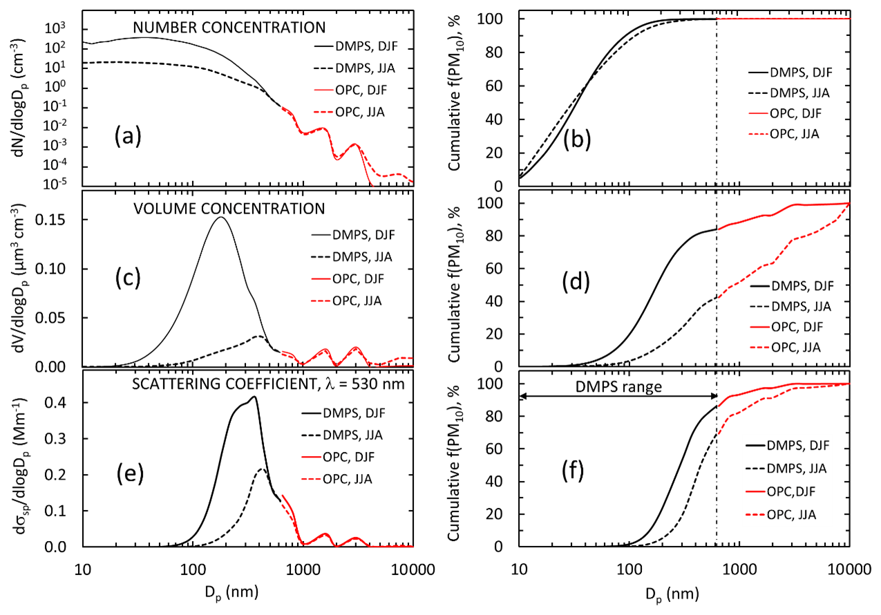
Figure 2 Average particle size distributions in summer (DJF) and in winter (JJA) in December 2007–July 2009 when both the DMPS and the Grimm OPC were operational. Left: average and median (a) number, (c) volume, and (e) scattering size distributions at λ=530 nm; right (b, d, f): cumulative fractions of the respective parameters in the size range D_p<7.5 µm, which corresponds to the aerodynamic particle size range D_a<9.8 µm.

Figure 2 shows the average particle number, volume, and scattering size distributions at λ=530 nm in the size range 10 nm–10 µm and the respective normalized cumulative size distributions in the size range of 10 nm–7.5 µm during the period from 14 December 2007 to 14 July 2009 in summer and in winter. Figure 2a and b show that for the number concentrations the OPC size range plays an insignificant role, whereas the larger particles contribute significantly to both total particle volume concentration (Fig. 2c and d) and scattering coefficients (Fig. 2e and f), and that this contribution varies seasonally. The contributions of fV(DMPS) and fσ_sp(DMPS,λ) were calculated for hourly averaged size distributions from Eqs. (3) and (7), and the monthly seasonal statistics were calculated and presented in Table 1 and as a box plot in Fig. 3. Both the table and the box plot show that both fV(DMPS) and fσ_sp(DMPS,λ) have maxima in summer and minima in winter. They also show that the ranges are large. Consequently, the use of the monthly averages presented in Table 1 for calculating m(DMPS,PM₁₀) and σ_sp(DMPS,PM₁₀), Eqs. (4) and (8), creates an additional uncertainty in the results. Another important result is that the wavelength dependency of fσ_sp(DMPS,λ) is clear, and it also has a seasonal cycle.

Figure 3 Seasonal cycle of the contribution of the size range measured by the DMPS to (a) volume concentration and (b) scattering coefficient at the PSAP wavelengths in December 2007–July 2009 when both the DMPS and the Grimm OPC were operational. The circle shows the average, the horizontal line the median, the box the 25th to 75th percentile range, and the whiskers the 5th to 95th percentile range in each month.

The wavelength dependency of the scattering coefficient can be described by the scattering Ångström exponent

$$\begin{array}{}\text{(9)}& {\mathit{\alpha }}_{\text{sp}}=-{\displaystyle \frac{\ln \left({\mathit{\sigma }}_{\text{sp}}\left({\mathit{\lambda }}_{\mathrm{1}}\right)/{\mathit{\sigma }}_{\text{sp}}\left({\mathit{\lambda }}_{\mathrm{2}}\right)\right)}{\ln \left({\mathit{\lambda }}_{\mathrm{1}}/{\mathit{\lambda }}_{\mathrm{2}}\right)}}\end{array}$$

that was calculated by using the wavelength pair $\mathrm{467}/\mathrm{660}$ nm. The variable names α_sp(DMPS,PM_0.8) and α_sp(DMPS,PM₁₀) will be used below for α_sp calculated from σ_sp(DMPS,PM_0.8) and σ_sp(DMPS,PM₁₀), respectively.

2.3.3 Absorption coefficients and equivalent black carbon concentrations

The PSAP data were first corrected for flow and spot size. The flow was calibrated 37 times during 2007–2013 with a TSI flow meter. The slopes and offsets of the calibrations were interpolated for each hour, and the PSAP flows were corrected accordingly. All absorption coefficients were corrected to STP (1013.25 hPa and 273.15 K).

The PSAP measures signal and reference detector counts, and the respective sums, ∑SIG and ∑REF, are used for calculating a non-scattering-corrected absorption coefficient, here σ_ap,nsc, from

$$\begin{array}{}\text{(10)}& \begin{array}{rl}& {\mathit{\sigma }}_{\text{ap,nsc}}=f\left(\text{Tr}\right){\displaystyle \frac{A}{Q\mathrm{\Delta }t}}\text{ln}\left({\displaystyle \frac{{\left(\sum _{\mathrm{\Delta }\mathrm{t}}\text{SIG}/\sum _{\mathrm{\Delta }t}\text{REF}\right)}_{t-\mathrm{\Delta }t}}{{\left(\sum _{\mathrm{\Delta }t}\text{SIG}/\sum _{\mathrm{\Delta }\mathrm{t}}\text{REF}\right)}_{\mathrm{t}}}}\right)\\ & =f\left(\text{Tr}\right){\mathit{\sigma }}_{\mathrm{0}},\end{array}\end{array}$$

where A is the filter spot area, Q the flow rate, Tr = ($\mathrm{\Sigma }\text{SIG}/\mathrm{\Sigma }\text{REF}{)}_t/(\mathrm{\Sigma }\text{SIG}/\mathrm{\Sigma }\text{REF}{)}_{t=\mathrm{0}}$ the transmittance, f(Tr) the loading correction function, and Δt the count integration time. The PSAP reports σ_ap,nsc with a 0.1 Mm⁻¹ resolution at a 1 s time resolution. Averaging the 1 s data is not good enough since at Dome C absorption coefficients are most of the time clearly lower than 0.1 Mm⁻¹. Therefore, the signal and reference counts ΣSIG and ΣREF were used in Eq. (10) with Δt=60 min. Manufacturer-cut spots of the standard filter material Pallflex E70-2075W were used in the PSAP. The spot diameter was measured to be 4.9±0.1 mm, so the spot area A was 18.9±0.6 mm². The uncertainty of A is ∼3 %.

Transmittance is reduced mainly by light absorption but also by scattering aerosol, which results in the so-called apparent absorption and has to be taken into account in the data processing. There are different algorithms for processing PSAP data, e.g., by Bond et al. (1999), Virkkula et al. (2005), Müller et al. (2014), and Li et al. (2020). Here we will use both the algorithms presented by Bond et al. (1999) (here B1999) with the adjustment presented by Ogren (2010),

$$\begin{array}{}\text{(11)}& \begin{array}{rl}& {\mathit{\sigma }}_{\text{ap}}={\displaystyle \frac{\mathrm{1}}{\mathrm{1.22}}}\left({\displaystyle \frac{\mathrm{0.97}\cdot \mathrm{0.873}}{\mathrm{1.0796}\cdot \text{Tr}+\mathrm{0.71}}}{\mathit{\sigma }}_{\mathrm{0}}-\mathrm{0.02}\cdot {\mathit{\sigma }}_{\text{sp}}\right)\\ & ={\displaystyle \frac{\mathrm{1}}{\mathrm{1.5557}\cdot \text{Tr}+\mathrm{1.0227}}}{\mathit{\sigma }}_{\mathrm{0}}-\mathrm{0.0164}\cdot {\mathit{\sigma }}_{\text{sp}}={\mathit{\sigma }}_{\text{ap,nsc}}\\ & -\mathrm{0.0164}\cdot {\mathit{\sigma }}_{\text{sp}},\end{array}\end{array}$$

and the algorithm presented by Virkkula et al. (2005) with the constants updated by Virkkula (2010) (here V2010):

$$\begin{array}{}\text{(12)}& {\mathit{\sigma }}_{\text{ap}}=\left(k_{\mathrm{0}}+k_{\mathrm{1}}(h_{\mathrm{0}}+h_{\mathrm{1}}{\mathit{\omega }}_{\mathrm{0}})\ln \left(\text{Tr}\right)\right){\mathit{\sigma }}_{\mathrm{0}}-s\cdot {\mathit{\sigma }}_{\text{sp}},\end{array}$$

where

$$\begin{array}{}\text{(13)}& {\mathit{\omega }}_{\mathrm{0}}={\mathit{\sigma }}_{\text{sp}}/\left({\mathit{\sigma }}_{\text{sp}}+{\mathit{\sigma }}_{\text{ap}}\right)\end{array}$$

is the single-scattering albedo and k₀, k₁, h₀, h₁, and s are wavelength-dependent constants. In the rest of the paper the symbol σ_ap,nsc will be used to present the non-scattering-corrected absorption coefficient, corrected with the constants and formula in Eq. (11) excluding the subtraction of σ_sp.

Since there are the above-explained size-dependent uncertainties of the scattering coefficient, additional absorption coefficient estimates were calculated by using both algorithms. The upper estimates of absorption coefficients σ_ap(σ_sp(DMPS,PM_0.8)) were calculated by using the lower estimate of the scattering coefficient σ_sp=σ_sp(DMPS,PM_0.8) in the scattering corrections in Eqs. (11) and (12), and the lower estimates of the absorption coefficient σ_ap(σ_sp(DMPS,PM₁₀)) were calculated by using the upper estimate of the scattering coefficient σ_sp=σ_sp(DMPS,PM₁₀) in the scattering corrections. Consequently, the lower and upper estimates of ω_o are denoted ω_o(σ_sp(DMPS,PM_0.8)) and ω_o(σ_sp(DMPS,PM₁₀)), respectively. They were calculated by using both Eqs. (11) and (12) for calculating σ_ap.

Considering that the period with the simultaneous measurements with the DMPS and the OPC showed that the DMPS size range always leads to an underestimation of both aerosol mass and scattering coefficient, it is likely that σ_ap corrected for scattering with σ_sp(DMPS, PM₁₀) is closer to the true σ_ap than that corrected with σ_sp(DMPS, PM_0.8). In the results σ_ap,nsc, σ_ap(σ_sp(DMPS,PM_0.8)), and σ_ap(σ_sp(DMPS,PM₁₀)) will be presented to evaluate the effect of using only the size range measured with the DMPS for the scattering correction.

Similarly to σ_sp, the wavelength dependency of light absorption by particles can roughly be described by the absorption Ångström exponent

$$\begin{array}{}\text{(14)}& {\mathit{\alpha }}_{\text{ap}}=-{\displaystyle \frac{\ln \left({\mathit{\sigma }}_{\text{ap}}\left({\mathit{\lambda }}_{\mathrm{1}}\right)/{\mathit{\sigma }}_{\text{ap}}\left({\mathit{\lambda }}_{\mathrm{2}}\right)\right)}{\ln \left({\mathit{\lambda }}_{\mathrm{1}}/{\mathit{\lambda }}_{\mathrm{2}}\right)}}\end{array}$$

that was calculated by using λ= 467 and 660 nm for σ_ap,nsc, σ_ap(σ_sp(DMPS,PM₁₀)), and both Eqs. (11) and (12). The variable names α_ap(σ_ap,nsc), α_ap(σ_sp(DMPS,PM₁₀),B1999), and α_ap(σ_sp(DMPS,PM₁₀),V2010, respectively, will be used to denote the α_ap calculated in different ways. These calculations were conducted to study the uncertainty of α_ap due to scattering corrections.

The absorption coefficient was used to estimate the concentration of equivalent black carbon, eBC (Petzold et al., 2013), from

$$\begin{array}{}\text{(15)}& \text{eBC}={\displaystyle \frac{{\mathit{\sigma }}_{\text{ap}}}{\text{MAC}}},\end{array}$$

where MAC is the mass absorption coefficient. For freshly emitted BC the MAC value is approximately 7.5 m² g⁻¹ at λ=550 nm (Bond et al., 2013). By assuming a wavelength dependency of λ⁻¹, this corresponds to MAC ≈7.8 m² g⁻¹ at λ=530 nm. This can be considered to yield an upper estimate for eBC concentrations since for coated BC particles MAC is larger (Bond et al., 2013). eBC was calculated by using σ_ap,nsc and σ_ap(σ_sp(DMPS,PM₁₀)) calculated with both algorithms, Eqs. (1) and (2). The corresponding variable names eBC(σ_ap,nsc) and eBC(σ_sp(DMPS,PM₁₀)) will be used below for them. The scattering-corrected eBC(σ_sp(DMPS,PM₁₀)) can be considered to be closer to the true eBC concentration. The reason for also presenting eBC(σ_ap,nsc) is that an estimate of BC concentrations is often needed even if it is known that it is an upper estimate (Caiazzo et al., 2021). It is also comparable with the eBC often presented from Aethalometer measurements. Presenting both yields a quantitative estimate of the bias due to not correcting the data for scattering.

The eBC mass fractions in the two size ranges D_a<0.8 and D_a<10 µm were calculated from

$$\begin{array}{}\text{(16)}& f\text{eBC}\left(m\left({\text{DMPS,PM}}_{\mathrm{0.8}}\right)\right)=\mathrm{100}\mathit{\%}{\displaystyle \frac{\text{eBC}}{m\left({\text{DMPS,PM}}_{\mathrm{0.8}}\right)}},\end{array}$$

$$\begin{array}{}\text{(17)}& f\text{eBC}\left(m\left({\text{DMPS,PM}}_{\mathrm{10}}\right)\right)=\mathrm{100}\mathit{\%}{\displaystyle \frac{\text{eBC}}{m\left({\text{DMPS,PM}}_{\mathrm{10}}\right)}},\end{array}$$

where the mass concentrations m(DMPS,PM_0.8) and m(DMPS,PM₁₀) were defined in Eq. (4) and eBC calculated from Eq. (15). Mass fractions were calculated for eBC(σ_ap,nsc) and eBC(σ_sp(DMPS,PM₁₀)).

2.3.4 Noise of scattering and absorption coefficients and eBC

The uncertainty of scattering coefficients should in principle be calculated from the error propagation formula ${\left(\mathit{\delta }{\mathit{\sigma }}_{\text{sp}}\right)}^{\mathrm{2}}=\sum {\left(\partial {\mathit{\sigma }}_{\text{sp}}/\partial x_i\right)}^{\mathrm{2}}{\left(\mathit{\delta }{x}_i\right)}^{\mathrm{2}}$, where δx_i is the uncertainty of variable x_i in calculating σ_sp (e.g., Sherman et al., 2015). That would require taking into account all uncertainties of the size distribution measurements and Mie modeling. However, a simplified approach was used here. The σ_sp calculated from the size distribution data and the uncertainty of the size distribution range were used for calculating lower and upper estimates of σ_sp as explained above. In addition to that, the noise of σ_sp was estimated from the average of the absolute differences of both consecutive hourly averaged scattering coefficients δσ_sp(average,1 h) = average(|Δσ_sp(1 h)|) = average(|σ_sp(t_i+1)–σ_sp(t_i)|). The average noise of 24 h averages was calculated from $\mathit{\delta }{\mathit{\sigma }}_{\text{sp}}\left(\mathrm{24}\text{h}\right)=\mathit{\delta }{\mathit{\sigma }}_{\text{sp}}\left(\text{average,1\hspace{0.17em}h}\right)/\sqrt{\mathrm{24}}$. The noises were calculated for both σ_sp(DMPS,PM_0.8)) and σ_sp(DMPS,PM₁₀). The noises are presented in Table 2. Note that the difference $\left|{\mathit{\sigma }}_{\text{sp}}\right(t_{i+\mathrm{1}})-{\mathit{\sigma }}_{\text{sp}}(t_i\left)\right|$ is not only due to random noise, so higher $\left|\mathrm{\Delta }{\mathit{\sigma }}_{\text{sp}}\right|$ values are observed when σ_sp is in reality increasing or decreasing, so the true random noise is slightly lower. When σ_sp is used in calculating the scattering correction of σ_ap in B1999 (Eq. 11), σ_sp is multiplied by 0.0164. Consequently, the σ_sp noise for the 24 h averages results in a 0.0164σ_sp noise for σ_ap. These noises are also presented in Table 2.

Table 2 Noise of scattering and absorption coefficients calculated from the particle number size distributions and the PSAP data for two averaging times (Δt=1 and 24 h). Noise was estimated for the scattering coefficients in the two size ranges (σ_sp(DMPS,PM_0.8) and σ_sp(DMPS,PM₁₀)) and for absorption coefficients without scattering corrections (σ_ap,nsc) and with scattering corrections (σ_ap(σ_sp(DMPS,PM_10.8)) and σ_ap(σ_sp(DMPS,PM₁₀))) as explained in Sect. 2.5.

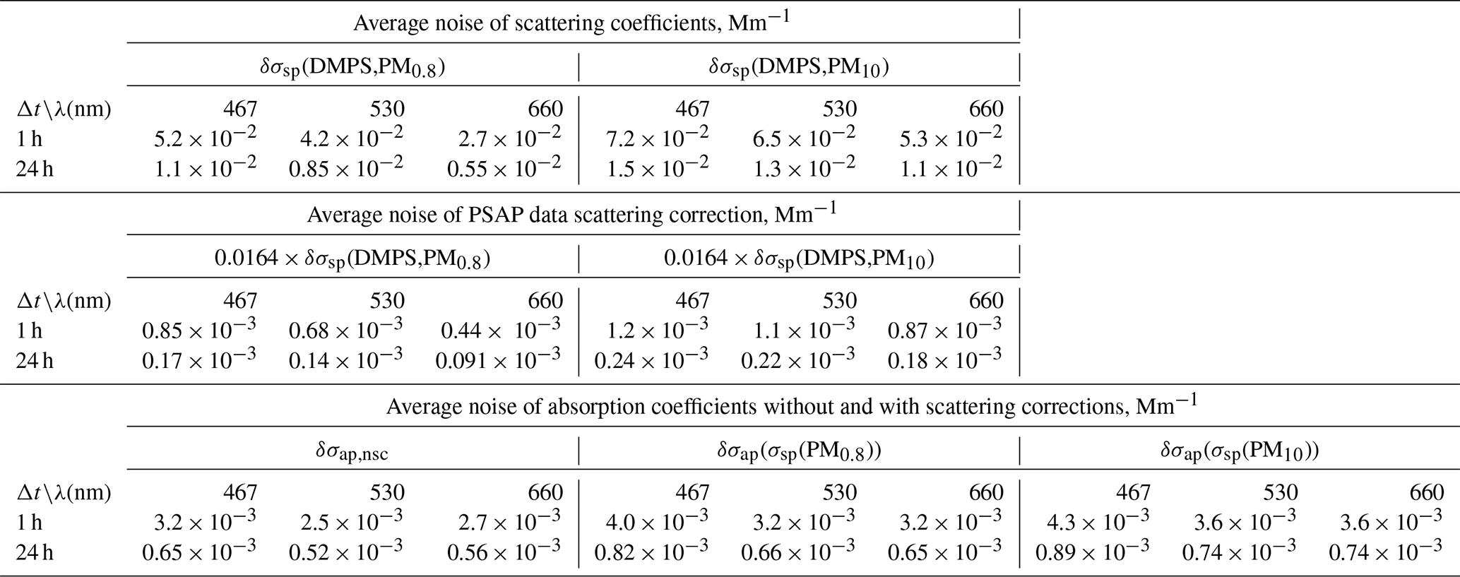
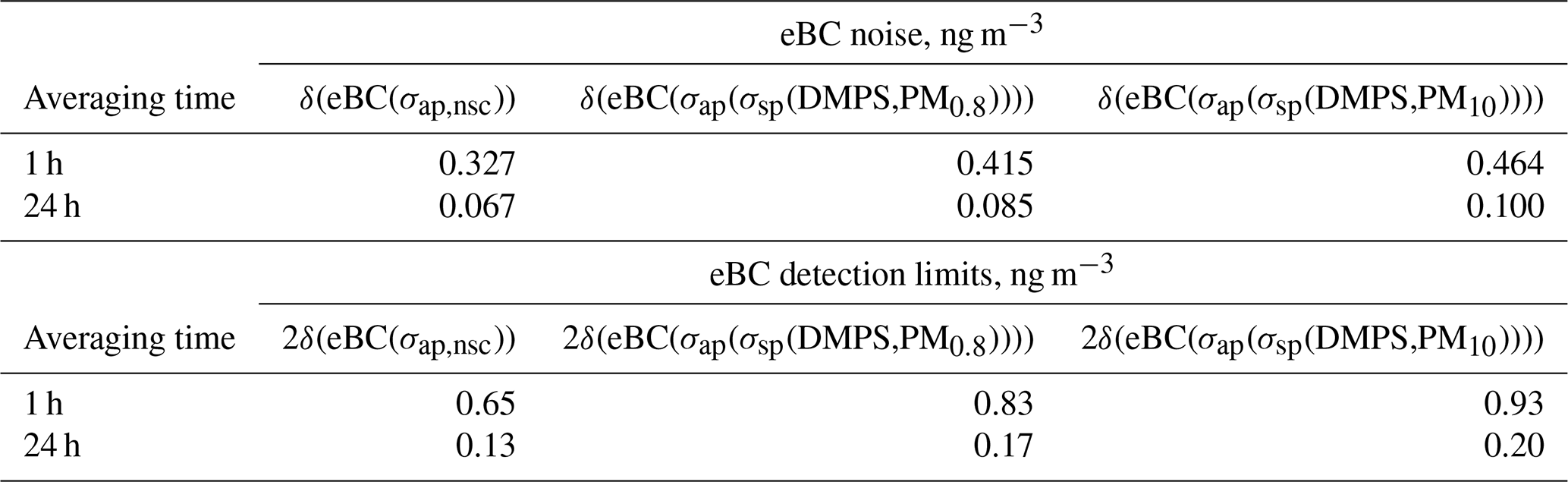
The uncertainty of the absorption coefficient should also be calculated from the error propagation formula, similarly to Sherman et al. (2015). However, here only the uncertainties of the spot size (∼3 %) and the statistical noise are taken into account. The noise of the non-scattering-corrected hourly σ_ap,nsc was estimated from the average of the absolute differences of both consecutive absorption measurements δσ_ap,nsc(average) = average($\left|\mathrm{\Delta }{\mathit{\sigma }}_{\text{ap,nsc}}\right|$) = average(|σ_ap,nsc(t_i)–σ_ap,nsc(t_i)|), similarly to the noise estimate of σ_sp. The noise of 24 h averages was estimated from $\mathit{\delta }{\mathit{\sigma }}_{\text{ap,nsc}}\left(\mathrm{24}\text{h}\right)=\mathit{\delta }{\mathit{\sigma }}_{\text{ap,nsc}}\left(\text{average,1\hspace{0.17em}h}\right)/\sqrt{\mathrm{24}}$. The noises in the scattering-corrected absorption coefficients were calculated from $\mathit{\delta }{\mathit{\sigma }}_{\text{ap}}=\mathit{\delta }{\mathit{\sigma }}_{\text{ap,nsc}}+$ 0.0164δσ_sp for both σ_ap(σ_sp(DMPS,PM_0.8)) and σ_ap(σ_sp(DMPS,PM₁₀)) and for 1 and 24 h averages (Table 2). The noise determined this way is formally correct only for σ_ap calculated with the B1999 formula, Eq. (11), not for V2010. However, calculated directly from the absolute differences, the average $\left|\mathrm{\Delta }{\mathit{\sigma }}_{\text{ap}}\right(\text{B1999}\left)\right|\approx$ average $\left|\mathrm{\Delta }{\mathit{\sigma }}_{\text{ap}}\right(\text{V2010}\left)\right|$, but the contribution of scattering to the noise was only determined for B1999, as explained above. For V2010, Eq. (12), a formal error propagation calculation is more complicated due to the iterative form of the procedure, and it is beyond the scope of the present paper. The noise of eBC was calculated from δ(eBC(σ_ap)) =δσ_ap $/$ MAC for both non-scattering-corrected and scattering-corrected eBC. The detection limits were defined as 2×δ(eBC(σ_ap)). The results are presented in Table 3.

The largest uncertainty factor for σ_ap, ω_o, α_ap, and eBC is not related to noise. It is due to the uncertainty of the refractive index and size distributions used for calculating σ_sp and the algorithm. This was evaluated by calculating σ_ap by using the lower and upper estimates of σ_sp in both scattering correction algorithms. These four values were used then for calculating ω_o, α_ap, and eBC, and they are presented below in relevant tables and figures.

2.4 Filtering and preprocessing the in situ data

Both PSAP absorption and DMPS-derived scattering coefficient data were filtered manually by removing rapidly changing values since they can be assumed to result from contamination from the station or from some technical problem. The PSAP transmittance data were used to filter out data measured at Tr <0.7 following recommendations in WMO/GAW Report No. 227 (2016) and the PSAP handbook (Springston, 2018). During most of 2010 the PSAP flow was extremely unstable, so practically the whole year was removed.

All major sources of light-absorbing aerosol other than the Dome C base are so far away that rapid variations in σ_ap,nsc are due to either instrument malfunction or influence from the base, for instance, emissions from vehicles. Further filtering of the data was done by removing data in which 10 min averages of σ_ap,nsc were more than 10 times larger than the hourly σ_ap,nsc. This was done to remove short events that are local but that do not appear to come directly from the base, based on wind direction. In all, roughly 13 % of the data were deemed contaminated.

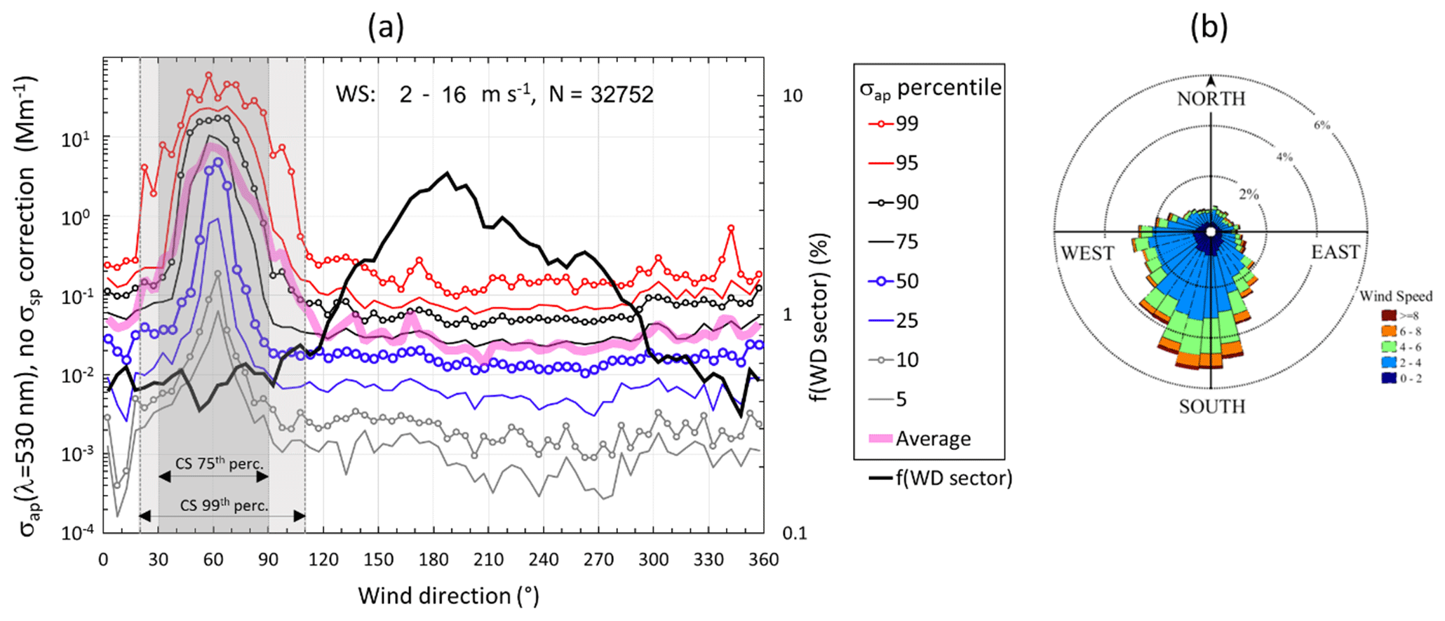
Figure 4 Wind and absorption coefficient. (a) Hourly averaged non-scattering-corrected absorption coefficients (σ_ap,nsc, Eq. 1) observed at wind speed WS > 2 m s⁻¹ in 5^∘ wind direction (WD) sectors. The lines present the percentiles of the cumulative σ_ap,nsc distribution in each WD sector. f(WD sector): fraction of wind data from each sector. CS 75th perc.: contamination sector determined from the 75th percentiles of the cumulative σ_ap,nsc distribution. CS 99th perc.: contamination sector determined from the 99th percentiles of the cumulative σ_ap,nsc distribution. (b) Distribution of WS and WD as a wind rose.

Additionally, wind data were used to remove clear contamination from the station. The sampling site is located upwind of the base itself by the prevailing wind directions. The base has a year-round diesel generator, and vehicles operated within the base area move around the base from November to February. Figure 4 shows the distribution of σ_ap,nsc in 5^∘ wind direction (WD) sectors at wind speed WS >2 m s⁻¹. The generator at the base is clearly observed as a pronounced peak of σ_ap,nsc at WD 60^∘. If the 75th percentile of the σ_ap,nsc cumulative distribution were used as the criterion for the contaminated sector when the wind direction was $\mathrm{30}{}^{\circ }<\text{WD}<\mathrm{90}{}^{\circ }$, then 6 % of the data would be filtered. If the 99th percentile of σ_ap,nsc is used, the contamination sector is wider, $\mathrm{20}{}^{\circ }<\text{WD}<\mathrm{110}{}^{\circ }$, and 10 % of the data would be filtered. Here the latter, i.e., the stricter criterion, was used. The distribution of σ_ap,nsc in the same WD sectors at several wind speed intervals is shown in Supplement Fig. S1. It is obvious that at low wind speeds contaminated air can come from all directions. Therefore, when WS <2 m s⁻¹, all data were filtered out, regardless of WD.

Table 3 Noise and detection limits of eBC concentrations calculated from the noise of the absorption coefficients presented in Table 2.

Since the size distribution and absorption measurements are done in the same cabin, the DMPS and OPC data were also removed when the PSAP observations indicated contamination. Figure 1 shows the instruments' operational time in hours. The DMPS measurements had more gaps than the PSAP. The three instruments required for a valid measurement were not always operational at the same time. After filtering, altogether 15 815 h of data remained for the statistical analyses. No filtering was applied to the PM₁ and PM₁₀ filter samples. The contamination is mainly BC, so it was to be assumed that the effect on ion concentrations was not significant.

The calculations were done using hourly averaged data. These data were filtered to remove contaminated data as explained above. The filtered data were then averaged over 24 h to reduce noise and improve detection limits. In the discussions below, the running 24 h averages were used, centered at each hour, i.e., σ_ap(t,24 H) = average(${\mathit{\sigma }}_{\text{ap}}(t-\mathrm{12},\mathrm{1}\text{H}),\mathrm{\dots },{\mathit{\sigma }}_{\text{ap}}(t+\mathrm{11},\mathrm{1}\text{H}$)), which means, for instance, that at noon ${\mathit{\sigma }}_{\text{ap}}(t=\mathrm{12},\mathrm{24}$ H) = average(${\mathit{\sigma }}_{\text{ap}}(t=\mathrm{0},\mathrm{1}$ H), …, ${\mathit{\sigma }}_{\text{ap}}(t=\mathrm{23},\mathrm{1}$ H)), so the noon average represents all absorption coefficients measured during that day. If, during any period to be averaged, there were less than 12 h of non-contaminated data, then that 24 h average was excluded from further analysis.

2.5 Filter sample analyses and data processing

There were two samplers in the immediate vicinity of the cabin where the other in situ measurements were made. There was a PM₁₀ sampling head operating following the CSN EN 12341 European Standard. The PM₁ samples were collected on the backup filter of a Dekati PM₁₀ impactor. In both of these, particles were sampled on Teflon filters (Pall-Gelman, 47 mm diameter, 2 µm nominal porosity). PM₁₀ and PM₁ load is obtained by summing the mass of the ions determined on Teflon filters. Note that this can be considered to be the lower estimate since there could be unidentified compounds, such as organic carbon on the filters.

Just before the analysis, half of each filter was extracted with 10 L of ultrapure water (18 M Ω Milli-Q) in an ultrasonic bath for 20 min. Every filter manipulation was carried out under a class-100 laminar-flow hood to minimize contamination risks. Inorganic anions and cations, as well as selected organic anions, were simultaneously measured by using a three Thermo Scientific Dionex ion-chromatograph (IC) system, equipped with electrochemically suppressed conductivity detectors. The sample handling during the IC injection was minimized by using a specifically designed Flow-Injection Analysis (IC-FIA) device (Morganti et al., 2007). Cations (Na⁺, NH${}_{\mathrm{4}}^{+}$, K⁺, Mg²⁺, and Ca²⁺) were determined by using a Thermo Scientific Dionex CS12A-4 mm analytical column with 20 mM H₂SO₄ eluent. Inorganic anions (Cl⁻, NO${}_{\mathrm{3}}^{-}$, SO${}_{\mathrm{4}}^{\mathrm{2}-}$, and C₂O${}_{\mathrm{4}}^{\mathrm{2}-})$ were measured by a Thermo Scientific Dionex AS4A-4 mm analytical column with a 1.8 mM Na₂CO${}_{\mathrm{3}}/\mathrm{1.7}$ mM NaHCO₃ eluent. F⁻ and some organic anions (acetate, glycolate, formate, and methanesulfonate) were determined by a Thermo Scientific Dionex AS11 separation column by a gradient elution (0.075–2.5 mM Na₂B₄O₇ eluent). Further details on the ion chromatographic measurements are reported in Udisti et al. (2004) and Becagli et al. (2011, 2021). All concentrations were corrected to STP (1013.25 hPa and 273.15 K). The ion data used in the present work are a subset of the data from 2005 to 2013 that Becagli et al. (2021) used for an analysis of the relationships between non-sea-salt sulfate, MSA, biogenic sources, and environmental constraints.

In addition to calculating scattering coefficients from the DMPS data, PM₁ and PM₁₀ mass concentrations were also used for calculating scattering coefficients. The scattering coefficients were calculated by multiplying the mass concentrations by mass scattering efficiencies (MSEs) presented by Hand and Malm (2007). The PM₁₀ mass concentrations were multiplied by the mass scattering efficiency of 1.9 m² g⁻¹, and the PM₁ concentrations were multiplied by 3.6 m² g⁻¹. These are the MSE for “total mixed” aerosol and “fine mixed” aerosol in Table 5 in Hand and Malm (2007), respectively. It has to be kept in mind that the MSE values in the above-mentioned paper were derived from measurements in the continental USA, so they most likely have a high uncertainty when applied to the Dome C aerosol. The MSE values presented by Quinn et al. (2002) were used for calculating the scattering coefficient of nss sulfate in PM₁ filters.

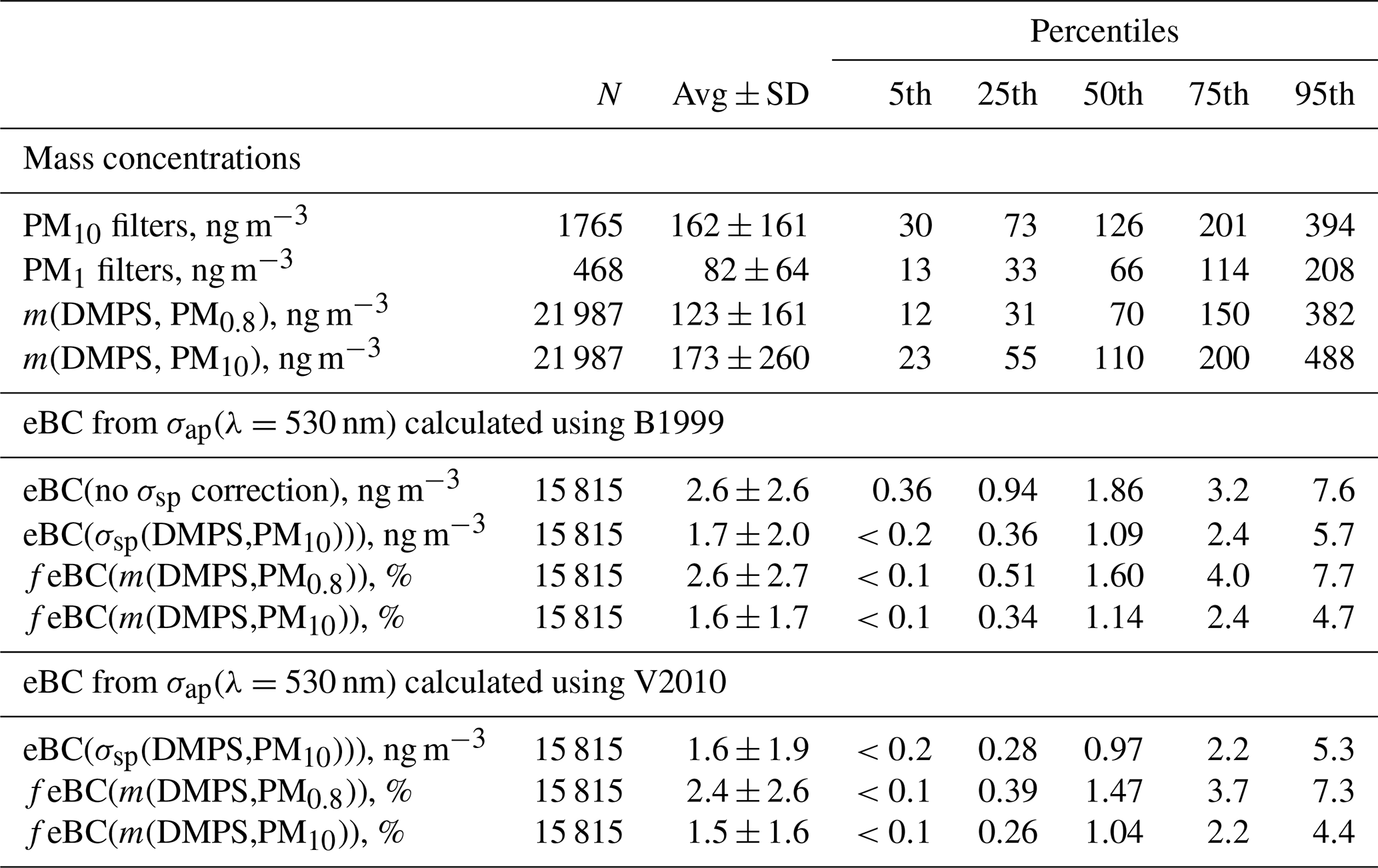
Table 4 Statistical summary of mass concentrations estimated from particle number size distributions, sums of ion concentrations of PM₁ and PM₁₀ filter samples, and the PSAP data at Dome C in 2008–2013. The statistical values of the PM₁ and PM₁₀ are those of all individual filters, and the statistical values calculated from the DMPS and PSAP data are those of running 24 h-averaged data; see details in the text. m(DMPS,PM_0.8): mass concentration calculated from the particle number size distributions measured with the DMPS assuming a particle density of 1.7 g cm⁻³; eBC: equivalent black carbon concentration calculated from the absorption coefficients at λ=530 nm calculated by using the B1999 algorithm without any scattering corrections and with B1999 and V2010 algorithms using σ_sp=σ_sp(DMPS,PM₁₀) for the scattering corrections and assuming MAC = 7.78 m² g⁻¹. fPM_0.8: scattering-corrected eBC mass fraction calculated from (eBC/m(DMPS,PM_0.8))×100 %; fPM₁₀: scattering-corrected eBC mass fraction calculated from (eBC/m(DMPS,PM₁₀))×100 %.

2.6 Scattering data from the South Pole

At the SPO the light-scattering coefficient has been measured for more than 40 years. An integrating nephelometer was installed in 1979 and used to measure σ_sp at four wavelengths (450, 550, 700, 850 nm). This nephelometer (Meteorology Research Inc. (MRI), Altadena, CA) was used until its failure in 2002, and a TSI Model 3563 three-wavelength nephelometer (λ=450, 550, and 700 nm) replaced it in November 2002 (Sheridan et al., 2016). Running 24 h averages of σ_sp(550 nm) were calculated for the years 2007–2013 the same way as was done for the Dome C data. The data were used for comparisons with σ_sp calculated from the Dome C data.

2.7 Source area analyses

The air-mass history and transport of aerosols to Dome C were calculated with the Lagrangian dispersion model FLEXPART (Stohl et al., 2005; Pisso et al., 2019). ECMWF reanalysis meteorology was used to run 60 000 trajectories every 6 h 50 d backwards from Dome C to make a statistical sampling of the air measured there. The FLEXPART trajectories follow the mean flow of the atmosphere plus random perturbations to account for turbulence.

In backward mode, the FLEXPART output is emission sensitivity S that is proportional to residence time within a grid cell (Stohl et al., 2005; Hirdman et al., 2010; Pisso et al., 2019). Depending on the settings, the output unit of FLEXPART in the backward runs can be s, s m³ kg⁻¹, or s kg m⁻³. In the present work the unit of S is seconds (s). When coupled with emissions, FLEXPART emission sensitivity creates a concentration at the release point that is equivalent to forward simulations from emissions, except for some small numerical differences (Seibert and Frank, 2004). One advantage of using a backward simulation in a case like this is that the emission sensitivity fields can be used not only to simulate concentrations, but also directly to quantitatively describe exactly where the air that reaches Dome C originates, and, thus, potential emissions influences. Emission sensitivity close to the surface – here at levels <1000 m a.g.l. – is often called the footprint (e.g., Hirdman et al., 2010). If a footprint were multiplied by emission mass flux in kg m⁻³ s⁻¹ at some grid cell, the result would be a concentration due to that emission at the receptor site (Stohl et al., 2005). In the present work, this step was not done.

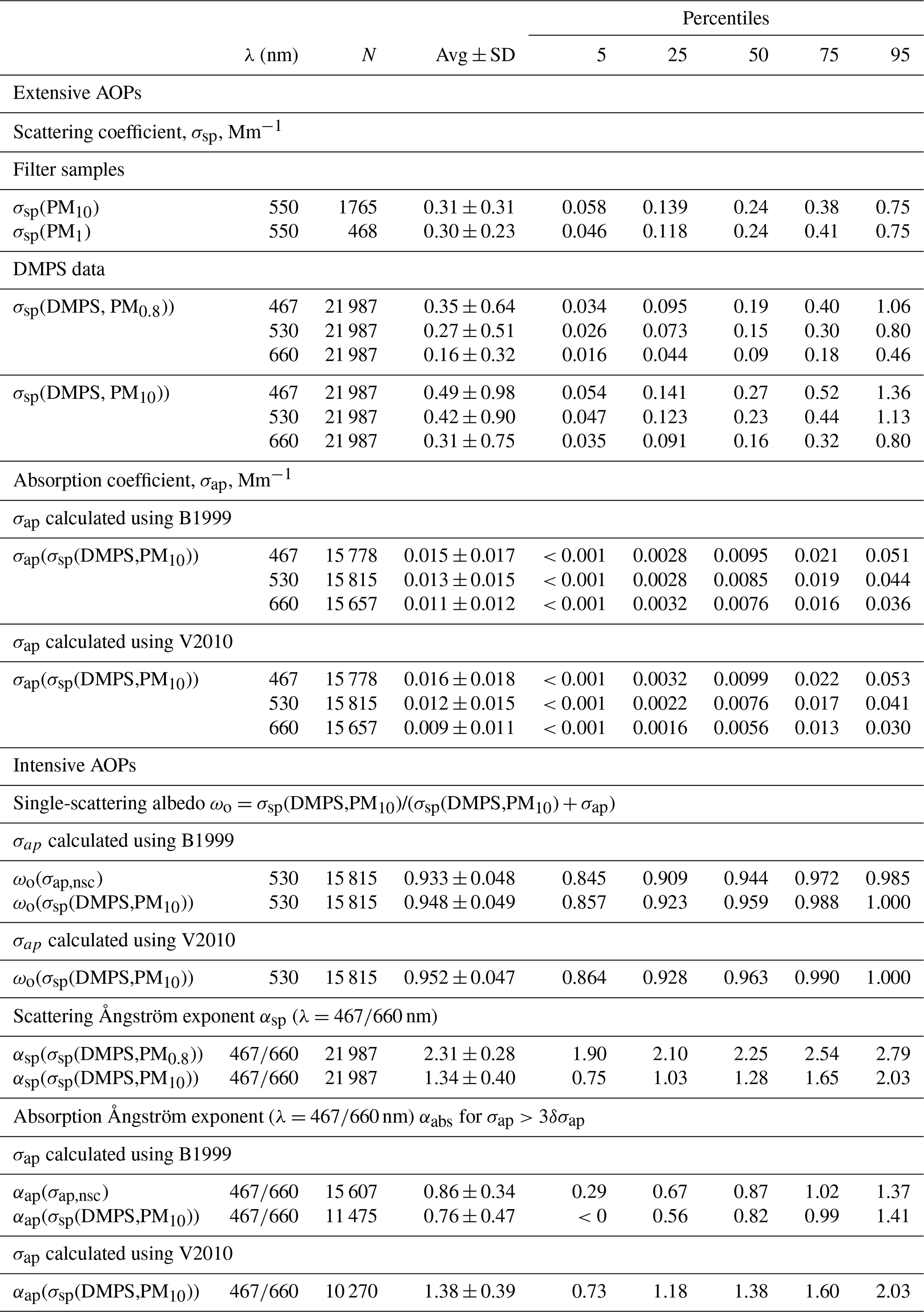
Table 5 Descriptive statistics of aerosol optical properties at Dome C in 2008–2013. The statistics were calculated from the 24 h running averages. λ: wavelength; N: number of data points used for the statistics, for filter sample number of filters. Avg ± SD: average ± standard deviation. See details and explanations of other symbols in the text.

To investigate the role of removal processes during transport, for all model runs, two different tracers were used, one atmospheric tracer with no removal and simulated BC particles with a lognormal size distribution (geometric mean diameter = 150 nm, geometric standard deviation 1.5) experiencing both dry and wet deposition. All tracers were run backwards for 50 d, in most cases sufficient for the aerosol tracer to have less than $\mathrm{1}\times {\mathrm{10}}^{-\mathrm{12}}$ of the emission sensitivity of the inert air tracer, meaning any emission prior to this would have been removed by the time of arrival at Dome C. The wet removal differentiates removal within and below clouds, also considering the water phase of the clouds and the precipitation type. The FLEXPART removal parameters are the efficiency of aerosols in serving as cloud condensation nuclei (CCN_eff) and ice nuclei (IN_eff). The values used for them were CCN_eff=0.9 and IN_eff=0.1 as in Table 4 of Grythe et al. (2017). The FLEXPART below-cloud scavenging is a scheme based on Laakso et al. (2003) and Kyrö et al. (2009), both described in Grythe et al. (2017). The model includes a realistic distribution of clouds by incorporating three-dimensional cloud information from ECMWF. For a detailed description, see Grythe et al. (2017).

2.7.1 Footprint difference calculations

A statistical analysis was applied to differentiate types of air pathways using a method derived from Hirdman et al. (2010). With the main aim of investigating the different pathways to Dome C, each 6 h interval was given a rank with regards to eBC concentration and single-scattering albedo. The emission sensitivity of the 50 d transport for an aerosol tracer was sorted according to its relative type. The emission sensitivities of the highest (S_H) and lowest (S_L) 10 % of eBC concentration and ω_o were calculated by averaging their emission sensitivities for a given grid cell I, j, and m by

$$\begin{array}{}\text{(18)}& S_{\ast }={\displaystyle \frac{\mathrm{1}}{M}}\sum _{m=\mathrm{1}}^{M}S\left(i,j,m\right),\end{array}$$

where M is the number of measurements and S_∗ can be any of the sorting criteria. The relative difference between two emission sensitivities S₁ and S₂ in percentage is then calculated as

$$\begin{array}{}\text{(19)}& {\text{RD}}_{\mathrm{1},\mathrm{2}}(i,j)=\mathrm{100}\mathit{\%}{\displaystyle \frac{S_{\mathrm{1}}(i,j)-S_{\mathrm{2}}(i,j)}{S_{\mathrm{1}}(i,j)+S_{\mathrm{2}}(i,j)}}.\end{array}$$

In the calculation the emission sensitivities close to the surface at <1000 m a.g.l. were used, and so Eq. (19) can be called the relative difference of footprints. This analysis of the footprints can be used to differentiate between different influencing factors on the air mass. This can be either the influence of transport, removal or combination of these (transport efficiency), or the emission strength.

2.7.2 Emissions used for interpreting the footprint statistics and observed seasonal cycles

The Global Fire Emissions Database (GFED) is a satellite information-based fire activity map. Monthly gridded burned area and emissions from fires are included in the product (http://www.globalfiredata.org, last access: 10 April 2022). Emitted BC is calculated based on emission factors, which depend on the type of vegetation that is burning. Satellites give snapshots collected to give pseudo global coverage and not continuous coverage. GFED v3.1 is based on the area burned, which is derived by coupling Moderate Resolution Imaging Spectroradiometer (MODIS) fire pixel counts with surface reflectance images (Giglio et al., 2006, 2009, 2010). This widely used emission inventory has uncertainties that arrive both from the emission factors and also from the amount of burnt material. A comparison of this bottom-up inventory with top-down inventories found large regional differences, and top-down estimates were about 30 % higher (Bond et al., 2013).

For the scattering aerosol two sources were considered. An offline tool (FLEX-SSA) developed by Grythe et al. (2014) and Grythe (2017) to simulate sea-spray aerosol (SSA) with FLEXPART was used. It uses inputs from the ECMWF model. These inputs are the wind speed at 10 m above the surface (U10) and the sea surface temperature (SST). The tool takes into account the sea ice fraction which is important to the Southern Ocean SSA emissions. The other major marine scattering aerosols discussed below are biogenic secondary aerosols. Behrenfeld et al. (2017) estimated monthly average phytoplankton biomass (C_phyto) concentrations in 2007–2015 from the Cloud-Aerosol Lidar with Orthogonal Polarization (CALIOP) satellite sensor data in three zones: Zone 1=45–55, Zone 2 = 55–65, and Zone 3 = 65–75^∘ S. The data provided by Michael J. Behrenfeld (2021, personal communication) were used for calculating seasonal monthly C_phyto averages in the three zones in 2008–2013. C_phyto can be used as a proxy of biological activity and emissions of dimethyl sulfide (DMS), a precursor of secondary biogenic aerosols.

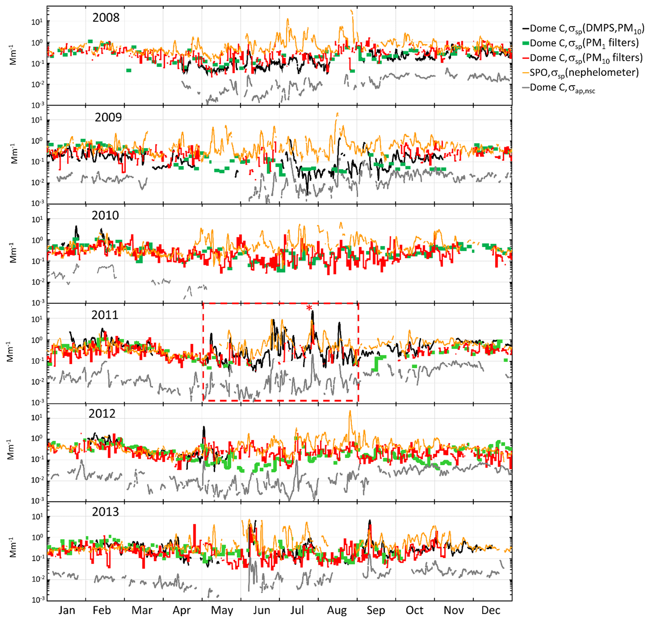
Figure 5 Time series of scattering coefficients calculated from the DMPS (σ_sp(DMPS,PM₁₀) at λ=530), PM₁ and PM₁₀ (λ=550) filter data measured at Dome C and measured with the nephelometer at the South Pole Station (SPO) (λ=550), and σ_ap,nsc(λ=530) measured with the PSAP at Dome C. The σ_sp from the DMPS and the nephelometer and σ_ap,nsc are running 24 h averages at each hour (±12 h), and the σ_sp from the PM₁ and PM₁₀ filters are those calculated for each filter. The red box within the 2011 time series shows the period presented in more detail in Fig. 6 and the red asterisk symbol (*) for which the footprint in Fig. 7 was calculated.

3 Results and discussion

3.1 Overview of the data

The time series of σ_sp calculated from the size distributions and from the PM₁ and PM₁₀ concentrations and the σ_ap,nsc at Dome C and σ_sp measured with the nephelometer at the SPO are presented in Fig. 5. For the DMPS-derived σ_sp only the upper estimate, σ_sp(DMPS,PM₁₀), Eq. (8) is shown. The descriptive statistics of aerosol optical properties and mass concentrations in the whole period are presented in Tables 4 and 5.

Several observations can be made from the time series in Fig. 5. First, the scattering coefficients calculated from the size distributions and the filter samples follow each other relatively well. There is a clear seasonal cycle of both σ_sp and σ_ap,nsc. It is clearly seen that σ_ap,nsc follows the temporal variations of σ_sp(DMPS): the high and low values occur mainly simultaneously, which is good considering that these two AOPs were measured with independent instruments. Since the PSAP and other filter-based absorption photometers are sensitive not only to absorbing but also scattering aerosol, and since Dome C is far from BC sources, it is possible that the good correlation is due to the apparent absorption only. Below, this will be studied simply by using Eqs. (11) and (12) to account for the scattering artifact in the absorption measurement.

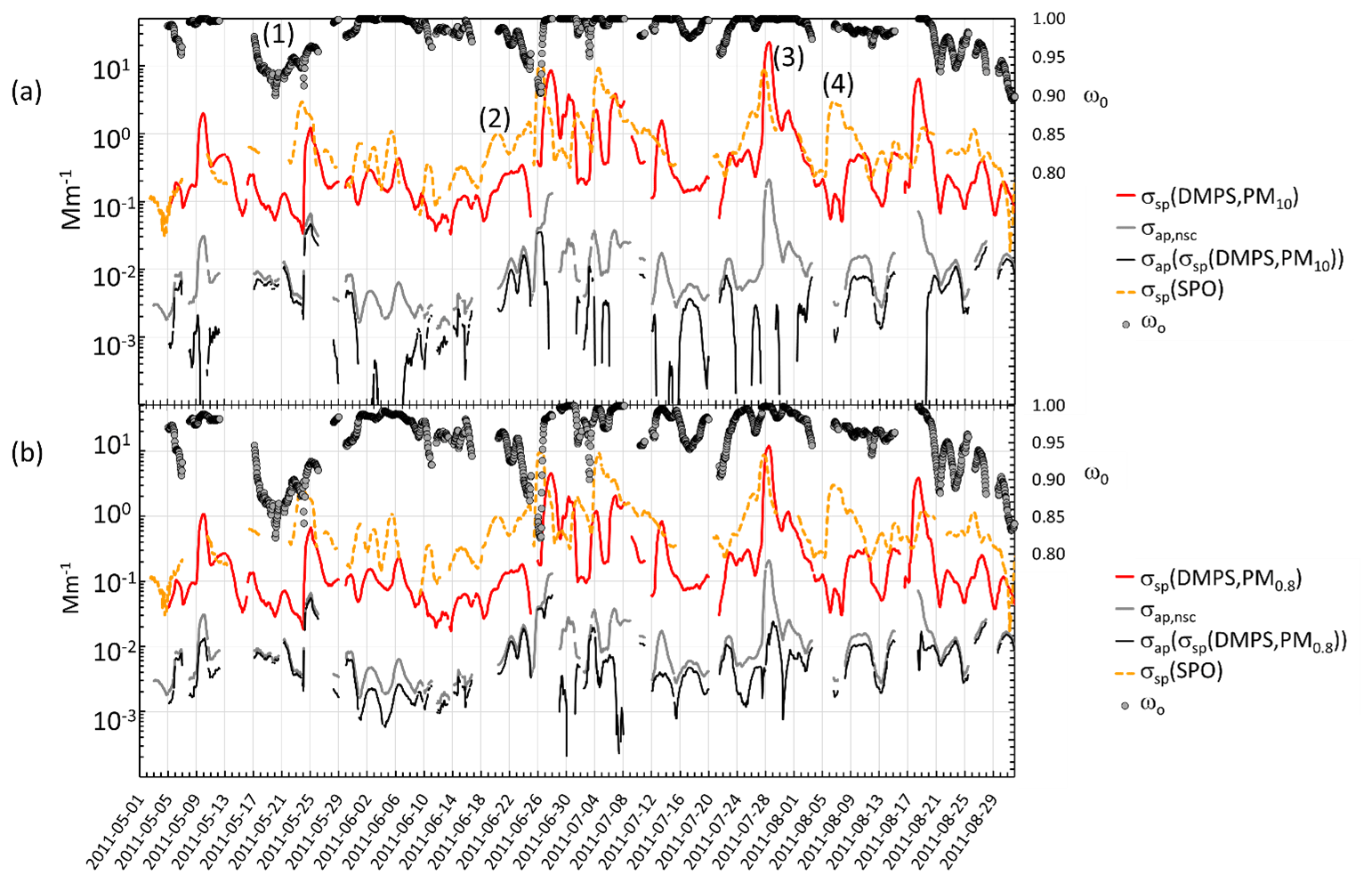
Figure 6 Four-month time series (May–August 2011) of σ_sp, σ_ap and ω_o at λ=530 nm at Dome C and σ_sp at λ=550 nm at the SPO: (a) upper estimate of σ_sp (=σ_sp(DMPS,PM₁₀)), lower estimate of σ_ap (=σ_ap(σ_sp(DMPS, PM₁₀))), and upper estimate of ω_o. (b) Lower estimate of σ_sp (=σ_sp(DMPS, PM_0.8))), upper estimate of σ_ap (=σ_ap(σ_sp(DMPS, PM_0.8))), and lower estimate of ω_o. In both (a) and (b) the non-scattering-corrected absorption coefficient is also shown. All values are running 24 h averages at each hour (±12 h). The numbers 1–4 are discussed in the text.

The σ_sp at Dome C and the SPO agrees better in austral summer than in winter. However, many high-concentration episodes are also observed in winter almost simultaneously at Dome C and the SPO. As an example, a 4-month period in May–August 2011 is presented in more detail in Fig. 6. The figure shows 24 h running averages of σ_sp, σ_ap, and ω_o at λ=530 nm at Dome C and σ_sp at λ=550 nm at the SPO. Figure 6a shows the upper estimate σ_sp=σ_sp(DMPS,PM₁₀), the corresponding lower estimate of σ_ap=σ_ap(σ_sp(DMPS,PM₁₀)) (corrected according to B1999, Eq. 11), and the upper estimate of ω_o. Figure 6b presents the lower estimate of σ_sp=σ_sp(DMPS,PM_0.8), the corresponding upper estimate of σ_ap=σ_ap(σ_sp(DMPS,PM_0.8)), and the lower estimate of ω_o. In both Fig. 6a and b the non-scattering-corrected absorption coefficient σ_ap,nsc is also shown.

In Fig. 6a, the period denoted by (1) shows an episode in which ω_o decreases significantly for several days, being an example of long-range-transported eBC. Episodes (2) and (3) are examples of periods when σ_sp is approximately an order of magnitude higher at the SPO than at Dome C. There are also events such as episode (3) when σ_sp is approximately the same at both sites. The peaks often seem to appear slightly earlier at the SPO than at Dome C, suggesting transport from the SPO to Dome C rather than the other way around. An example of this is shown in the footprint (Fig. 7) calculated for the episode denoted by (3) in Fig. 6. The footprint shows that the air masses came from the direction of the Antarctic peninsula via the SPO to Dome C. Air flow from the direction of the Weddell Sea to the SPO and then to Dome C is consistent with a very-long-known winter-time circulation pattern (Alt et al., 1959) as reviewed by Shaw (1979). During the event denoted by episode (3), σ_ap,nsc was also high. However, when the scattering correction (Eq. 11) was applied, the resulting σ_ap was not especially high and ω_o was in the range of 0.98–1.00 for both the upper and lower estimates of σ_sp, which indicates that non-scattering-corrected absorption coefficients may be considerably overestimated when σ_sp is high.

The scattering coefficients calculated from the size distributions, averaged over the filter sampling periods, correlate positively with the scattering coefficients calculated from the PM₁ and PM₁₀ filters (Fig. 8). Ordinary least squares regression was used here. The main purpose of the regression was to study whether there is a statistically significant correlation between the scattering coefficients calculated from the size distributions and the filter samples. According to the slopes 0.78±0.02 and 0.76±0.04 of the regression lines in Fig. 8a and c, σ_sp(DMPS, PM_0.8) also seems to be the lower estimate of σ_sp when it is compared with the filter-sample-derived σ_sp. According to the slope of 1.29±0.04 in Fig. 8b, σ_sp(DMPS, PM₁₀) is an upper estimate of σ_sp compared with σ_sp(PM₁₀), but when σ_sp(DMPS, PM₁₀), it is compared with σ_sp(PM₁) and the slope is 1.01±0.06, which appears to be somewhat controversial. There are also other peculiarities in the scatter plots. The scatter plots of σ_sp(DMPS, PM_0.8) vs. σ_sp(PM₁₀) (Fig. 8a) have data points where σ_sp(DMPS) is low, in the range of ∼0.02–0.03 Mm⁻¹, but σ_sp(PM₁₀) varies in a much larger range from ∼0.02 to ∼0.9 Mm⁻¹. This also occurs when σ_sp(DMPS, PM₁₀) is compared with σ_sp(PM₁₀) (Fig. 8b). The pattern could be explained by too low values of both σ_sp(DMPS, PM_0.8) and σ_sp(DMPS, PM₁₀) or by too high values of σ_sp(PM₁₀). A similarly suspicious pattern is not observed in the comparison with the PM₁ filters (Fig. 8c and d), suggesting the problem may be with σ_sp(PM₁₀). It is clear that this is not a calibration of either the size-distribution-derived or filter-sample-derived σ_sp, but the main message of the regressions is that the values are of the same order of magnitude and that there is a statistically significant positive correlation between them which increases confidence in the results. When the regressions are compared with each other, it has to be kept in mind that the sampling periods and the number of samples of the PM₁ and PM₁₀ data were not the same.

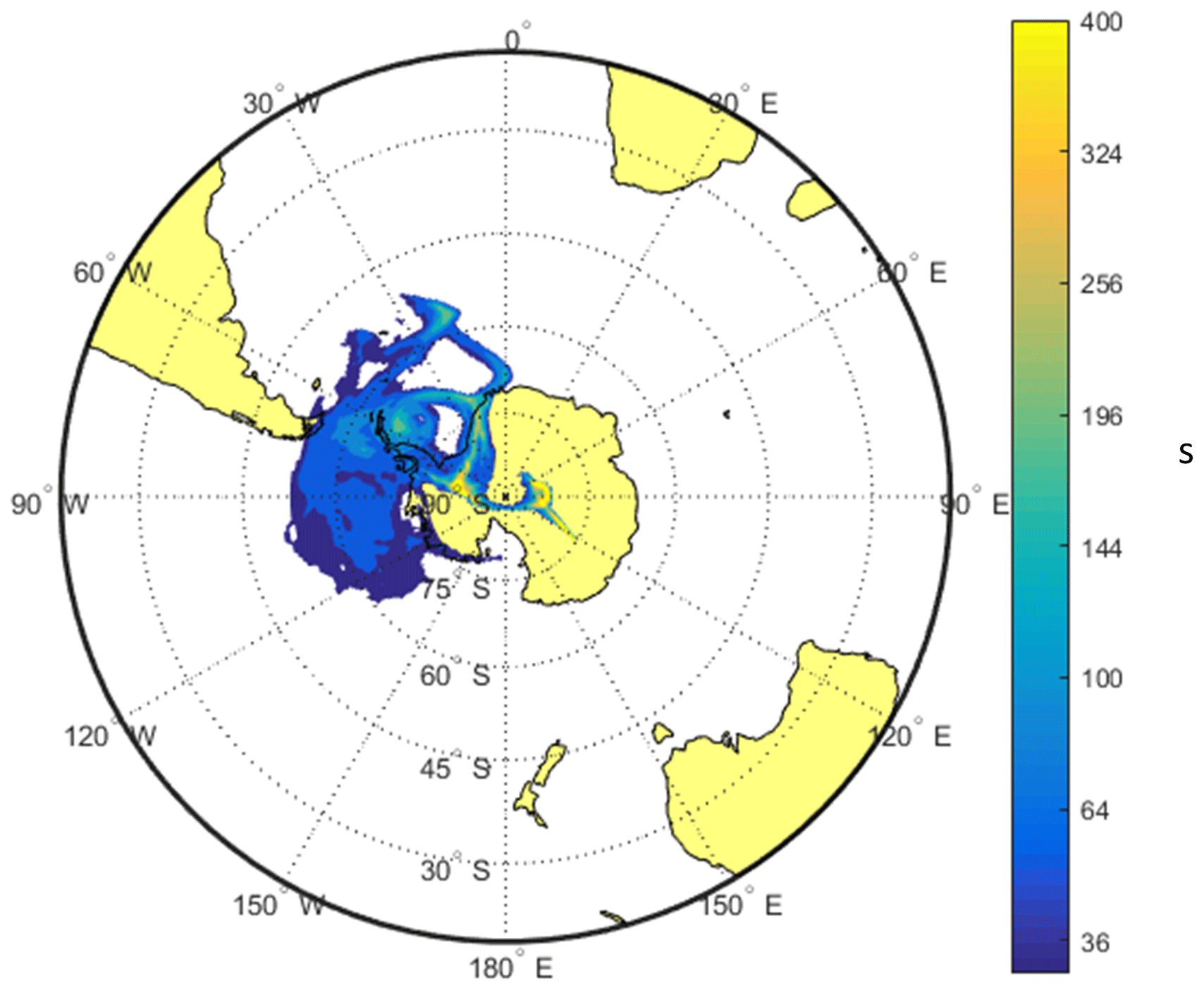
Figure 7 FLEXPART footprint of the overall highest day of scattering in winter 2011, on 28 July 2011, indicated by the number (3) in Fig. 6.

Other reasons for the wide scatter of the data points are the mass scattering efficiencies (MSEs) used for calculating scattering coefficients from the filter samples (see Sect. 2.5), uncertainties in ion analyses from the filters, and uncertainties in calculating scattering coefficients from the size distributions, especially the estimation of σ_sp(DMPS,PM₁₀) from size distributions measured with the DMPS only. In spite of all these uncertainties, the statistical values (averages and percentiles of the cumulative distributions) of the scattering coefficients are reasonably similar. For instance, the medians of σ_sp(PM₁₀, λ=550 nm), σ_sp(PM₁, λ=550 nm), σ_sp(DMPS, PM_0.8, λ=530 nm), and σ_sp(DMPS, PM₁₀, λ=530 nm) were 0.24, 0.24, 0.15, and 0.23 Mm⁻¹, respectively (Table 4). The fact that the medians of σ_sp(PM₁₀) and σ_sp(PM₁) are the same is somewhat suspicious: it would be expected that σ_sp(PM₁)<σ_sp(PM₁₀). At this point it is worth paying attention to the statistics of the mass concentrations calculated from the size distributions and from the sum of ions in the filter samples (Table 5). The median mass concentrations of the PM₁ and PM₁₀ filters were 66 and 126 ng m⁻³, respectively, in the expected order. These mass concentrations are also in reasonably good agreement with the median m(DMPS, PM_0.8) of 70 ng m⁻³ and median m(DMPS, PM₁₀) of 110 ng m⁻³ (Table 5). This suggests that the MSE values used for calculating scattering coefficients from the filter masses were not correct. As was written in Sect. 2.5, the MSE values were taken from Hand and Malm (2007), who derived them from measurements conducted mainly in US national parks. Considering this, the agreement of the filter-sample-derived with size-distribution-derived σ_sp is reasonable.

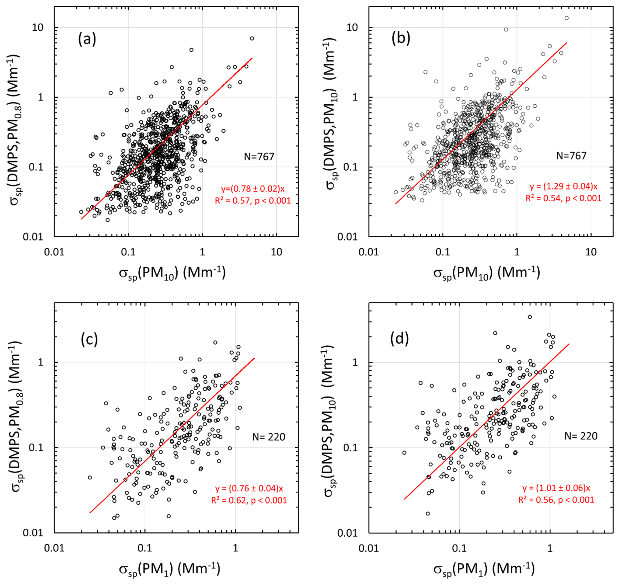
Figure 8 Comparison of scattering coefficients calculated from the DMPS vs. scattering coefficients calculated from the PM₁ and PM₁₀ filter sample data at Dome C, all at λ=550 nm. The scattering coefficients calculated from the DMPS data were averaged for the sampling times of the PM₁ and PM₁₀ samples and interpolated to λ=550 nm. (a) Lower estimate of σ_sp (=σ_sp(DMPS, PM_0.8)) vs. σ_sp(PM₁₀), (b) upper estimate of σ_sp(=σ_sp(DMPS,PM₁₀)) vs. σ_sp(PM₁₀), (c) σ_sp(DMPS, PM_0.8)) vs. σ_sp(PM₁), and (d) σ_sp(DMPS,PM₁₀)) vs. σ_sp(PM₁). N: number of data points. The red line shows the linear regression line that is forced through zero. The regression equations show the slope ± standard error of the slope, the squared correlation coefficient, and the p value of the slope.

3.2 Seasonal cycles of AOPs

3.2.1 Seasonal cycles of scattering and absorption coefficients

The seasonal cycles of scattering and absorption coefficients are presented in Fig. 9. The SPO scattering coefficients presented in Fig. 9a–d were measured using the TSI nephelometer, and the Dome C scattering coefficients were calculated using the PM₁ (Fig. 9a) and PM₁₀ (Fig. 9b) filter sample data as explained in Sect. 2.5 and from the number size distributions (Fig. 9c–d). The maximum and minimum monthly average and median scattering coefficients were observed in austral summer and winter, respectively. At the SPO the scattering coefficient was similar to that at Dome C in austral summer, but there was a large difference in austral winter. At the SPO the maximum monthly average scattering coefficients were observed in austral winter but at Dome C in austral summer. This suggests that in austral winter SPO is more influenced by sea-spray emissions than Dome C. However, even though the averages and medians are lower at Dome C, high scattering coefficients are also occasionally observed there in austral winter, as is shown by the 95th percentiles in Fig. 9c and d and above in the time series of winter 2011 (Fig. 6). The data do not explain the reasons for the difference between Dome C and the SPO in austral winter. It may either be due to different geographical locations, different size ranges measured by the instruments, or both.

A hypothetical explanation for the difference between the scattering coefficients at the SPO and Dome C could be that in the very dry conditions the particles are not spherical. It is true that the shape of particles affects light scattering. However, it mainly affects the polarization of scattered light: spherical particles do not change the state of the polarization of scattered light, but nonspherical particles do. This is used, for example, in polarization lidars to discriminate ice crystals, dust particles, and droplets. However, integral photometric characteristics, such as extinction, scattering, and absorption cross sections and single-scattering albedo, do not depend significantly on particle shape, as is shown in chapter 10 of the textbook by Mischenko et al. (2002). Therefore, nonsphericity is not a likely explanation for the difference.

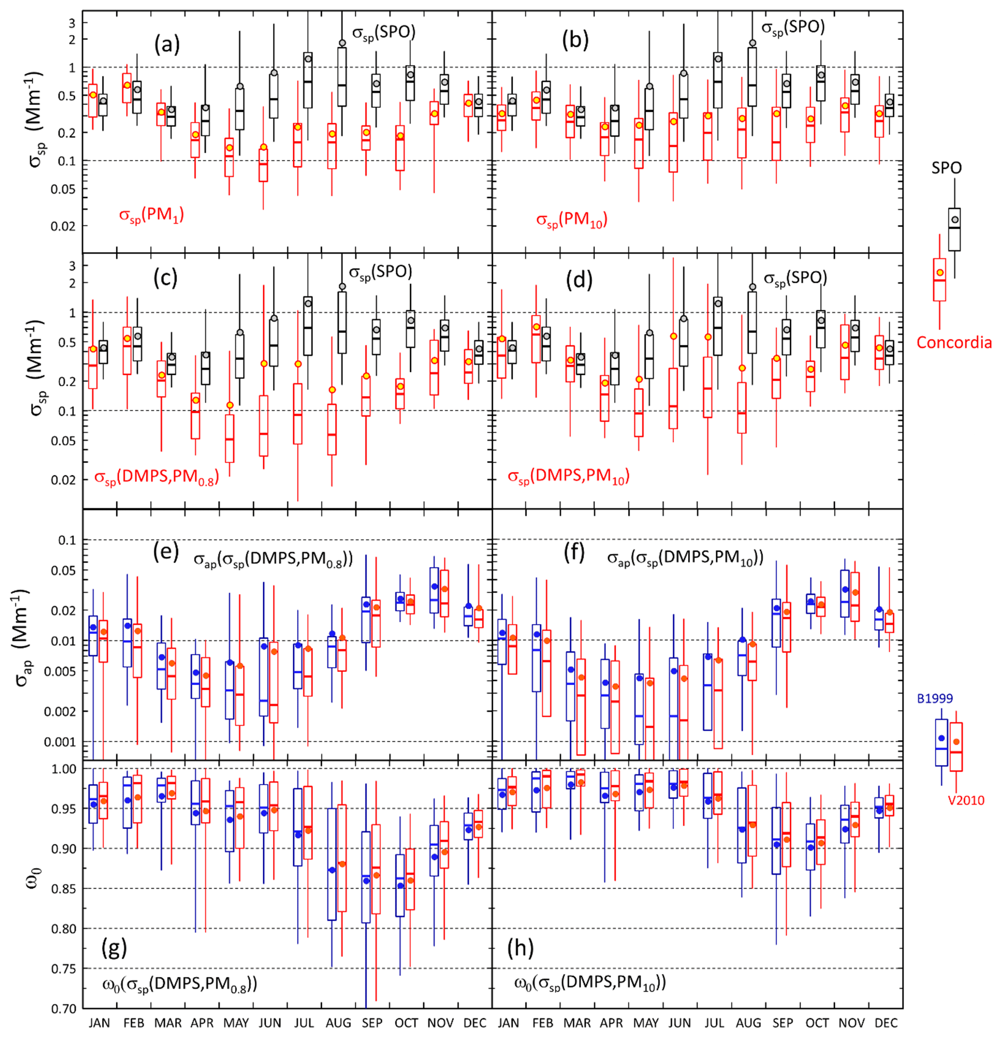
Figure 9 Seasonal cycles of scattering and absorption coefficients and single-scattering albedo. (a) Scattering coefficient (σ_sp) calculated from the sums of analyzed ion concentrations in PM₁ filters at λ=550 nm, (b) σ_sp calculated from the sums of analyzed ion concentrations in PM₁₀ filters, (c) the lower estimate of σ_sp=σ_sp(DMPS,PM_0.8), (d) the upper estimate of σ_sp=σ_sp(DMPS,PM₁₀), (e) absorption coefficient σ_ap calculated with the algorithms of B1999 and V2010 (Eqs. 17 and 18) by using the σ_sp lower estimate for scattering correction, (f) σ_ap calculated with the two algorithms by using the σ_sp upper estimate for scattering correction, (g) single-scattering albedo ω_o calculated by using the σ_sp lower estimate for both σ_sp and σ_ap, and (h) ω_o calculated by using the σ_sp upper estimate for both σ_sp and σ_ap.

The minimum monthly means and medians of σ_ap at Dome C were observed in austral autumn (MAM) and the maximum monthly means and medians in austral spring (SON), which is different than the seasonal cycle of σ_sp (Fig. 9e and f, Tables S2 and S4). As a result, the seasonal cycle of the single-scattering albedo ω_o is such that the darkest aerosol, i.e., the lowest ω_o, is observed in September and October and the highest ω_o in February and March (Fig. 9g and h, Table S5). When the lower estimate for σ_sp (i.e., σ_sp(DMPS, PM_0.8)) is used for the scattering correction (Eqs. 11 and 12), the October monthly medians of ω_o are 0.862 and 0.868 when using the B1999 and V2010 algorithms, respectively, and when the upper estimate σ_sp(DMPS, PM₁₀) is used for the scattering corrections, the October monthly medians of ω_o are 0.911 and 0.916 when using the B1999 and V2010 algorithms, respectively (Table S5). The highest monthly median single-scattering albedos are ∼0.98 and >0.99 with both algorithms when using the σ_sp lower and upper estimates for the scattering corrections, respectively. These results show that when σ_sp is not measured but calculated from the size distributions, the σ_ap and ω_o are clearly less sensitive to the selection of the algorithm (B1999 or V2010) than to the scattering coefficient used for the scattering correction. However, as was noted in Sect. 2.3.4, it is likely that σ_ap(σ_sp(DMPS,PM₁₀)) is closer to the true absorption coefficient than σ_ap(σ_sp(DMPS,PM_0.8)), so we can also consider the seasonal cycles presented in Fig. 9d, f, and h to be the closest to the true ones.

3.2.2 Seasonal cycles of scattering and absorption Ångström exponents

The wavelength dependency of both scattering and absorption have clear seasonal cycles. The average scattering Ångström exponent of particles in the DMPS size range, α_sp(DMPS,PM_0.8), varies from ∼2.6 in austral summer (DJF) to ∼2.1 in austral winter (JJA), indicating that in austral summer the size distributions are dominated by smaller particles than in winter (Fig. 10a, Table S3). This cycle is much clearer when α_sp is calculated from the upper estimate of scattering: average α_sp(DMPS,PM₁₀) varies from ∼1.9 in austral summer to ∼0.8 in winter. The seasonal cycle of α_sp(DMPS,PM₁₀) is actually strikingly similar to the seasonal cycle of α_sp of σ_sp measured at the SPO. This supports the use of the wavelength-dependent formula (Eq. 8) for calculating σ_sp(DMPS,PM₁₀,λ) from σ_sp(DMPS,PM_0.8,λ). The range of α_sp is much larger at the SPO than at Dome C, however. The main reason is probably that when σ_sp(DMPS,PM₁₀,λ) was calculated with Eq. (8), only the monthly averages of fσ_sp(DMPS,λ) (Eq. 7) were used, but the fσ_sp(DMPS,λ) range is actually quite large (Fig. 3). The SPO values were calculated from direct PM₁₀ scattering measurements from a nephelometer.

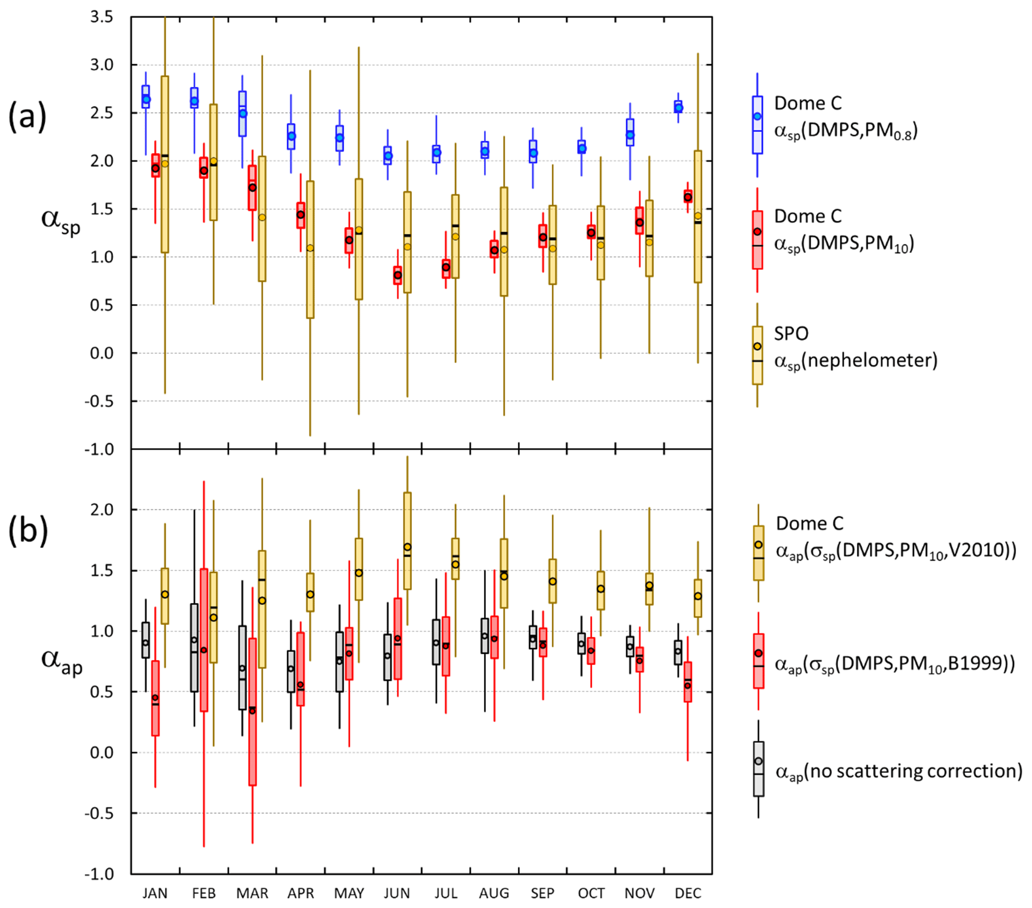
Figure 10 Seasonal cycles of the wavelength dependency of (a) scattering and (b) absorption. In panel (a) the Ångström exponent α_sp was calculated from the size distributions measured at Dome C (σ_sp(DMPS,PM_0.8) and σ_sp(DMPS,PM₁₀) for the wavelength range 467–660 nm and measured at the South Pole Station with a nephelometer. The SPO α_sp was calculated for the wavelength range 550–700 nm. In panel (b) the absorption Ångström exponent α_ap was calculated for the σ_ap without scattering correction and by using the B1999 and V2010 algorithms with scattering corrected using σ_sp=σ_sp(DMPS,PM₁₀). In all of them the data with σ_ap>3δσ_ap were used.

The absorption Ångström exponent α_ap was calculated for the non-scattering-corrected absorption coefficient σ_ap,nsc and for the scattering-corrected σ_ap(σ_sp(DMPS,PM₁₀)) with the two algorithms. Close to the σ_ap detection limit the ratios of σ_ap at two wavelengths are very noisy, so Fig. 10b and Tables 4 and S6 present α_ap statistics of absorption coefficients for ${\mathit{\sigma }}_{\text{ap}}>\mathrm{3}\times \mathit{\delta }{\mathit{\sigma }}_{\text{ap}}$, where δσ_ap is the wavelength-dependent 24 h average noise at λ=467 and λ=660 nm (Table 2). Note that the number of accepted data points is lower for the scattering-corrected than non-scattering-corrected α_ap (Table 4). The reason is that the scattering correction often decreases σ_ap below 3×δσ_ap.

The first observation that can be made from looking at the statistics (Fig. 10b, Tables 4 and S6) is that α_ap(σ_sp(DMPS,PM₁₀),V2010) is always larger than α_ap(σ_ap,nsc) and α_ap(σ_sp(DMPS,PM₁₀),B1999). The main explanation for this is that the constants in the V2010 algorithm (Eq. 12) depend on wavelength, but the B1999 algorithm (Eq. 11) uses the same constants for all wavelengths. The differences between the α_ap obtained from different algorithms were also discussed by Backman et al. (2014) and Luoma et al. (2021).

The seasonal cycles of α_ap(σ_ap,nsc) and α_ap(σ_sp(DMPS,PM₁₀),B1999) are qualitatively similar: the lowest medians are observed in March and the maxima in August–October. This cycle is approximately anticorrelated with the ω_o seasonal cycle: in March the median ω_o is the highest, and the lowest is in August–October. In March the median α_ap(σ_ap,nsc) and α_ap(σ_sp(DMPS,PM₁₀),B1999) were ∼0.6 and 0.37 and in August–September 0.96 and ∼0.92–0.96, respectively (Table S6), essentially the value generally used for pure BC. The seasonal cycle of α_ap(σ_sp(DMPS,PM₁₀),V2010) is a little bit different: the minimum median of ∼1.2 is in February, and the maximum of ∼1.7 occurs in June (Table S6).

The interpretation of α_ap is complicated. The α_ap is related to the dominant absorbing aerosol type, but physical properties of the particles also affect it. For externally mixed BC particles it is generally assumed to be around 1 (Hegg et al., 2002; Bond and Bergstrom, 2006; Bond et al., 2013) and higher for some organic aerosol from biomass smoke and mineral dust (Kirchstetter et al., 2004; Russell et al., 2010; Devi et al., 2016). However, α_ap also depends on the size of BC cores and coating thickness. It is easy to show with Mie models that for single non-coated BC particles with $D_{\text{p}}<\sim \mathrm{20}$ nm, α_ap is indeed close to 1, but when D_p≈100 nm α_ap≈1.3 depending on the wavelength pair used for the calculation and <1 when D_p >∼150 nm. For BC particle size distributions the width and the dominant particle size affect α_ap. Coating of BC cores affects α_ap even more: when BC particles are coated either with a light-absorbing shell or even with a light-scattering shell, α_ap can be clearly larger than 1 (e.g., Gyawali et al., 2009; Lack and Cappa, 2010; Virkkula, 2021). Core-shell simulations of size distributions of BC particles coated with a light-scattering shell show that ${\mathit{\alpha }}_{\text{ap}}>\sim \mathrm{1.4}$ for the wavelength pair of $\mathrm{470}/\mathrm{950}$ nm could be obtained for BC particle size distributions when the shell volume fraction is $>\sim \mathrm{89}$ %–90 %, and the geometric mean diameter of the BC particles is in the range of ∼70–100 nm (Virkkula, 2021). Higher α_ap would also be obtained by coating with a light-absorbing shell such as brown carbon. In the present work such α_ap values were obtained for α_ap(σ_sp(DMPS,PM₁₀),V2010) for the wavelength pair $\mathrm{467}/\mathrm{660}$ nm. So, if these values are closer to the truth, it seems that the BC particles that are observed at Dome C are thickly coated and their dominant particle size is $<\sim \mathrm{100}$ nm. On the other hand, if the average α_ap≈0.8 obtained for α_ap(σ_ap,nsc) and α_ap(σ_sp(DMPS,PM₁₀),B1999) is closer to the truth, the core-shell simulation of Virkkula (2021) suggests that BC particle size distributions would be dominated by thinly coated particles in the size range >100 nm.

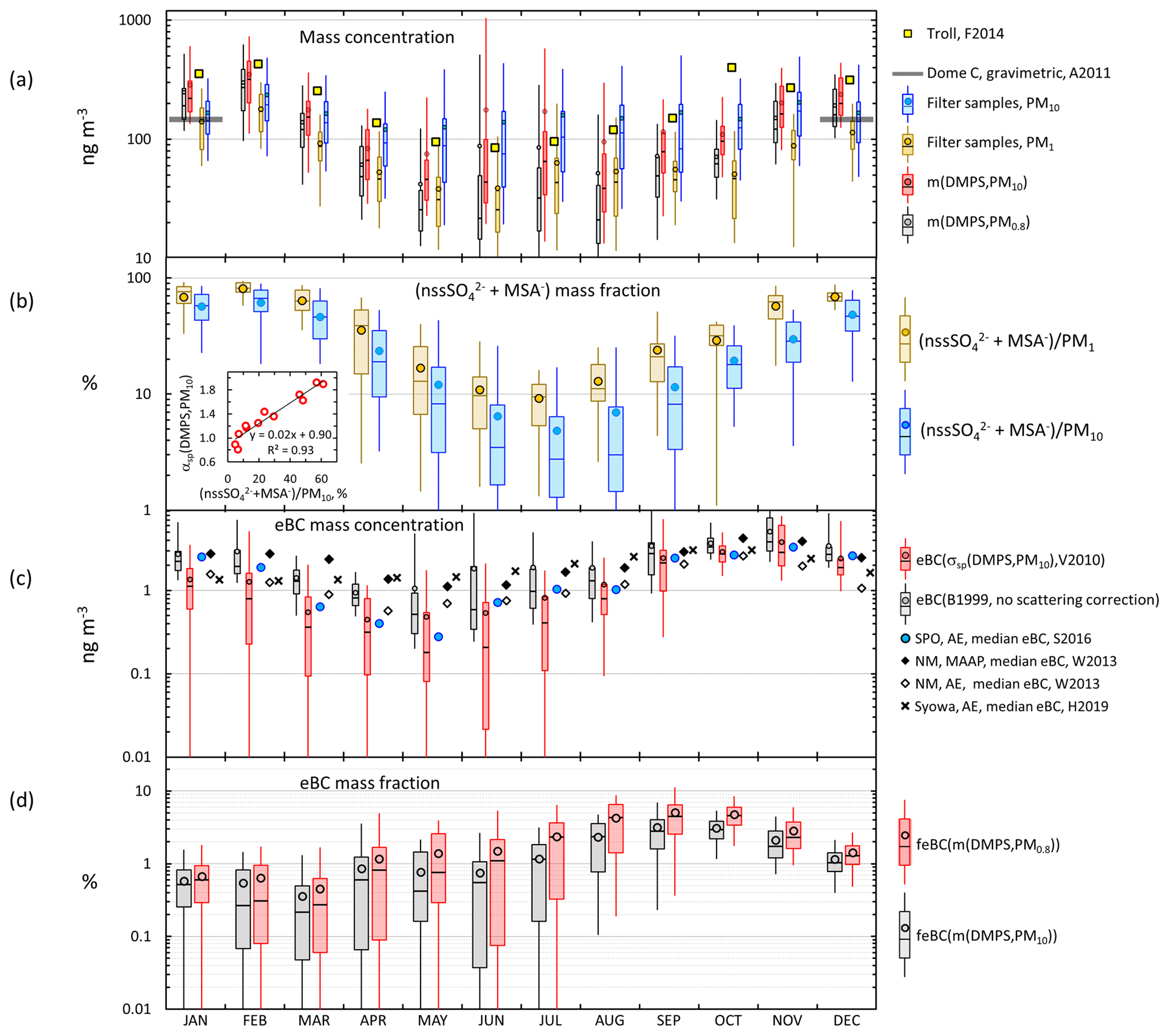
Figure 11 Seasonal cycles of (a) aerosol mass concentration calculated from the particle number size distributions m(DMPS,PM₁₀) and m(DMPS,PM_0.8), the sum of ions analyzed from PM₁ and PM₁₀ filters, (b) mass fraction of the sum of nssSO${}_{\mathrm{4}}^{\mathrm{2}-}$ and MSA in PM₁ and PM₁₀ filters, (c) equivalent black carbon (eBC) concentration calculated from the non-scattering-corrected absorption coefficients and from σ_ap corrected with the σ_sp upper estimate (σ_sp(DMPS,PM₁₀)), and (d) mass fraction eBC calculated as the ratio of eBC corrected with the σ_sp upper estimate to m(DMPS,PM_0.8) and m(DMPS,PM₁₀). Comparison values: (a) monthly average mass concentration calculated from particle volume concentrations at Troll (F2014: Fiebig et al., 2014), average gravimetric PM₁₀ mass concentration at Dome C (A2011: Annibaldi et al., 2011), and (c) monthly median eBC concentrations measured at Neumayer (NM) with a MAAP and an Aethalometer (AE) (W2013: Weller et al., 2013), at the SPO with an Aethalometer (S2016: Sheridan et al., 2016), and at Syowa with an Aethalometer (H2019: Hara et al., 2019). The small insert in panel (b) shows the scatter plot and linear regression of monthly average α_sp(DMPS,PM₁₀) vs. monthly average mass fraction of the sum of nssSO${}_{\mathrm{4}}^{\mathrm{2}-}$ and MSA in PM₁₀ filters.

3.3 Seasonal cycles of mass concentrations, eBC mass concentrations, and mass fractions

The seasonal cycles of the mass concentrations m(DMPS,PM_0.8) and m(DMPS,PM₁₀) (see Sect. 2.3.2), the mass concentrations of the PM₁ and PM₁₀ filter samples, the mass fraction of the sum of secondary sulfur ions, the eBC mass concentrations, and the eBC mass fractions feBC(m(DMPS,PM_0.8)) and feBC(m(DMPS,PM₁₀)) (Eqs. 16 and 17) are presented in Fig. 11 and in Tables S1, S7, S8, and S9. Some corresponding published Antarctic data are also plotted in Fig. 11 for comparison. The m(DMPS,PM_0.8) and the m(PM₁) are consistent with each other in that the minimum median mass concentrations are observed in May and June and the maximum medians in February. This cycle is very similar to that observed at the Norwegian station Troll in 2007–2011 (Fiebig et al., 2014). The monthly average volume concentrations of particles in the size range 33–830 nm in Fig. 9 of Fiebig et al. (2014) were digitized and multiplied by the same particle density ρ=1.7 g cm⁻³ that was used for the Dome C data and plotted in Fig. 11a. The average (± standard deviation) of the ratio m(DMPS,PM_0.8,Dome C)/m(DMPS,Troll) of the monthly averages is $\sim \mathrm{0.6}\pm \mathrm{0.2}$, i.e., about 40 % lower at Dome C. Fiebig et al. (2014) reasoned that the seasonal cycle of particles in the size range measured by the DMPS, i.e., m(DMPS), is controlled by photo-oxidation-limited aerosol formation. This is obviously true for Dome C also. In February, when the maximum monthly average PM₁ and PM₁₀ concentrations were observed, the contribution of the sum of secondary sulfur ions (nssSO${}_{\mathrm{4}}^{\mathrm{2}-}$ + MSA⁻) was also the highest (Fig. 11b): the average (± standard deviation) contributions to the sum of ions in the PM₁ and PM₁₀ filters was then $\sim \mathrm{81}\pm \mathrm{12}$ % and $\sim \mathrm{61}\pm \mathrm{23}$ %, respectively. The concentrations and the contributions of nssSO${}_{\mathrm{4}}^{\mathrm{2}-}+$ MSA⁻ were lowest in July, $\sim \mathrm{9}\pm \mathrm{5}$ % and $\sim \mathrm{5}\pm \mathrm{5}$ % for PM₁ and PM₁₀, respectively.

The seasonal cycle of larger particles (m(PM₁₀) and m(DMPS,PM₁₀)) is much weaker (Fig. 11a) than the m(PM₁) and m(DMPS,PM_0.8) cycle. The explanation is that the contribution of sea salt to aerosol mass is the highest in winter (Fig. 11b) and that a large fraction of sea-salt particles is in the supermicron size range, in line with other studies of aerosols at Dome C (e.g., Jourdain et al., 2008; Udisti et al., 2012; Legrand et al., 2017a, b). Note that the seasonal cycle of the mass fraction of secondary sulfur ions is qualitatively similar to the seasonal cycle of the scattering Ångström exponent α_sp (Fig. 10a): both have the highest values in the austral summer and the lowest values in the austral winter. This is especially clear for the PM₁₀ filters. The small insert in Fig. 11b shows the scatter plot of the monthly average α_sp(DMPS,PM₁₀) vs. $({\mathrm{nssSO}}_{\mathrm{4}}^{\mathrm{2}-}+{\mathrm{MSA}}^{-})/{\mathrm{PM}}_{\mathrm{10}}$. The relationship is essentially linear, and the correlation coefficient is high, r²=0.93. Since the usual interpretation of the size dependence of α_sp is that it is inversely proportional to the dominating particle size, it indicates that when the mass fraction of secondary aerosol is the highest, the dominating particle size is the smallest. As such this is not a surprising observation, but it is an additional piece of information that links the chemical composition and aerosol optical properties.

The estimated m(PM₁₀) values are consistent with the concentrations measured gravimetrically by Annibaldi et al. (2011) in December 2005–January 2006. The average PM₁₀ mass concentration they obtained was 134±12 ng m⁻³ at p=1013 hPa and T=298 K, which equals 146±12 ng m⁻³ at p=1013 hPa and T=273 K used in the present paper. The average (and median) PM₁₀ mass concentrations in the present work were 167 ng m⁻³ (140 ng m⁻³) and 167 ng m⁻³ (143 ng m⁻³) in December and January, respectively (Table S1), in good agreement with the gravimetric measurement of Annibaldi et al. (2011) even though their measurements were not conducted in the same period as ours.

In the austral summer the mass concentration calculated from the size distributions (m(DMPS,PM_0.8) and m(DMPS,PM₁₀)) were ∼100 ng m⁻³ higher than the sums of ions in the PM₁ and PM₁₀ filters (Table S1). Part of the explanation could in principle be that the density 1.7 g cm⁻³ used for calculating mass concentrations from the size distributions was too high, but it cannot explain all of it. Another possible explanation is that there were organic compounds not observed with ion chromatography. Caiazzo et al. (2021) took filter samples at Dome C in a different period, December 2016–January 2018, and analyzed them for organic and elemental carbon with an $\mathrm{OC}/\mathrm{EC}$ analyzer. The average OC concentration was 86±29 ng m⁻³, approximately the concentration difference between the size-distribution-derived ions and the sums of ions in the filter samples.

The eBC concentrations eBC(σ_ap,nsc) and eBC(σ_sp(DMPS,PM₁₀)) were calculated from Eq. (15). For the scattering-corrected σ_ap, the two algorithms, Eqs. (11) and (12), yielded essentially the same absorption coefficients at λ=530 nm. Therefore, only one of them is shown in the seasonal cycle plot in Fig. 11c, but both are presented in Supplement Table S7. On the other hand, eBC(σ_ap,nsc) is also plotted to show how much the scattering correction affects the calculated eBC concentrations in different seasons. For comparison, published monthly median eBC seasonal cycles at three other Antarctic sites are plotted in Fig. 11c: at Neumayer, a coastal site in Queen Maud Land, using two methods, an Aethalometer, and a MAAP (Weller et al., 2013), at Syowa, another Queen Maud Land coastal site using an Aethalometer (Hara et al., 2019), and at the SPO using an Aethalometer (Sheridan et al., 2016). The maximum median eBC concentrations are observed in October–November at all sites. The maximum eBC in October–November is $\sim \mathrm{3}\pm \mathrm{1}$ ng m⁻³, quite similar at all sites. For eBC it appears that there is no significant difference between the coastal and plateau sites. The highest monthly median eBC concentrations are those measured with the MAAP at Neumayer in October but, for the same month, the median Aethalometer-derived eBC at Neumayer is the lowest. The lowest monthly median eBC concentrations are observed in April–May at Neumayer, the SPO, and Dome C and 3 months earlier in February at Syowa. The lowest monthly medians, ∼0.2 and ∼0.3 ng m⁻³, were observed at Dome C and the SPO in May, respectively. The minima were higher at the coastal sites. Note, however, that the eBC concentrations measured with the Aethalometer in Fig. 11c were not corrected for scattering. This correction was done only for the PSAP data from Dome C and automatically for the MAAP data from Neumayer. After the corrections the Dome C monthly median eBC(σ_sp(DMPS,PM₁₀)) ranged from ∼0.2 in May to ∼3 ng m⁻³ in October–November, i.e., approximately by an order of magnitude and approximately the same as at the SPO. The range is smaller at the coastal sites. This might be due to not correcting for the scattering artifact even though the range of MAAP-derived eBC concentrations at Neumayer is also smaller than on the plateau sites.

The seasonal cycle of eBC is somewhat different from that of the mass concentration. Consequently, the minimum eBC mass fractions in both size ranges (feBC(m(DMPS,PM_0.8) and feBC(m(DMPS,PM₁₀)), Eqs. (16) and (17), were in February–March and the maxima in August–October (Fig. 11d, Tables S8 and S9). The eBC mass fractions during this peak were actually quite high. In particular, if it is assumed that all eBC is in the size range measured with the DMPS, even for the scattering-corrected eBC monthly medians and averages of feBC varied around 4 %–5 % and the 75th percentiles around 6 %–7 % by using both algorithms (Table S8). These are BC mass fractions typically observed in urban locations (e.g., Liu et al., 2014; Shen et al., 2018), in airborne measurements over Europe (McMeeking et al., 2010), and in biomass-burning plumes (Pratt et al., 2011), suggesting that in these periods a large fraction of aerosol was long-range-transported aerosol from other continents or highly processed air with larger, more scattering aerosol preferentially removed. The highest eBC monthly average and median mass concentrations were observed in November, but then feBC was lower than its maximum. This can be explained by the increase in the amount of new, non-absorbing natural secondary particles and condensational growth of BC cores by compounds originating from the sea austral during spring and summer. Järvinen et al. (2013) classified new particle formation (NPF) events observed at Dome C, and the highest fraction of new particle formation events was in November, while in austral spring the particle growth rate was also the highest. The minimum feBC monthly averages were $<\sim \mathrm{0.5}$ % and medians $<\sim \mathrm{0.3}$ % in February–March (Tables S8 and S9). This minimum also occurs simultaneously with the minimum eBC concentrations. This suggests that during this time of the year the amount of long-range transported aerosol from other continents is at a minimum at the same time when the biogenic aerosol production from the oceans is still high.

The seasonal cycles of single-scattering albedo (Fig. 9) and eBC mass fraction (Fig. 11d) are anticorrelated with each other. It is logical: the lower the feBC is, the higher the fraction of scattering aerosol and ω_o is. Their relationships can be used for assessing whether their observed seasonal cycles could be explained by internal mixing of BC particles and scattering components. Linear regressions of monthly average and median ω_o vs. feBC yield high correlation coefficients, but the regression lines would yield negative values at feBC = 100 %. So, an exponential function of the form of ω_o(feBC) =ω_o(feBC=0)exp($-k\cdot$ feBC) was fitted with the data (Fig. 12). The correlation coefficients were slightly worse, $\sim \mathrm{0.89}\pm \mathrm{0.01}$ for ω_o vs. feBC(m(DMPS,PM_0.8) (Fig. 12a), than the $\sim \mathrm{0.98}\pm \mathrm{0.01}$ for ω_o vs. feBC(m(DMPS,PM₁₀) (Fig. 12b). If the fitted exponential functions were valid up to feBC = 100 %, the ω_o(feBC(m(DMPS,PM_0.8) would predict that the average ω_o≈0.2 and the ω_o(feBC(m(DMPS,PM₁₀) would predict that ω_o (feBC = 100 %)≈0.06. These are reasonable values for pure BC: it has been measured that for fresh pure BC ω₀ is approximately 0.2±0.1 (e.g., Bond and Bergstrom, 2006; Mikhailov et al., 2006; Bond et al., 2013).

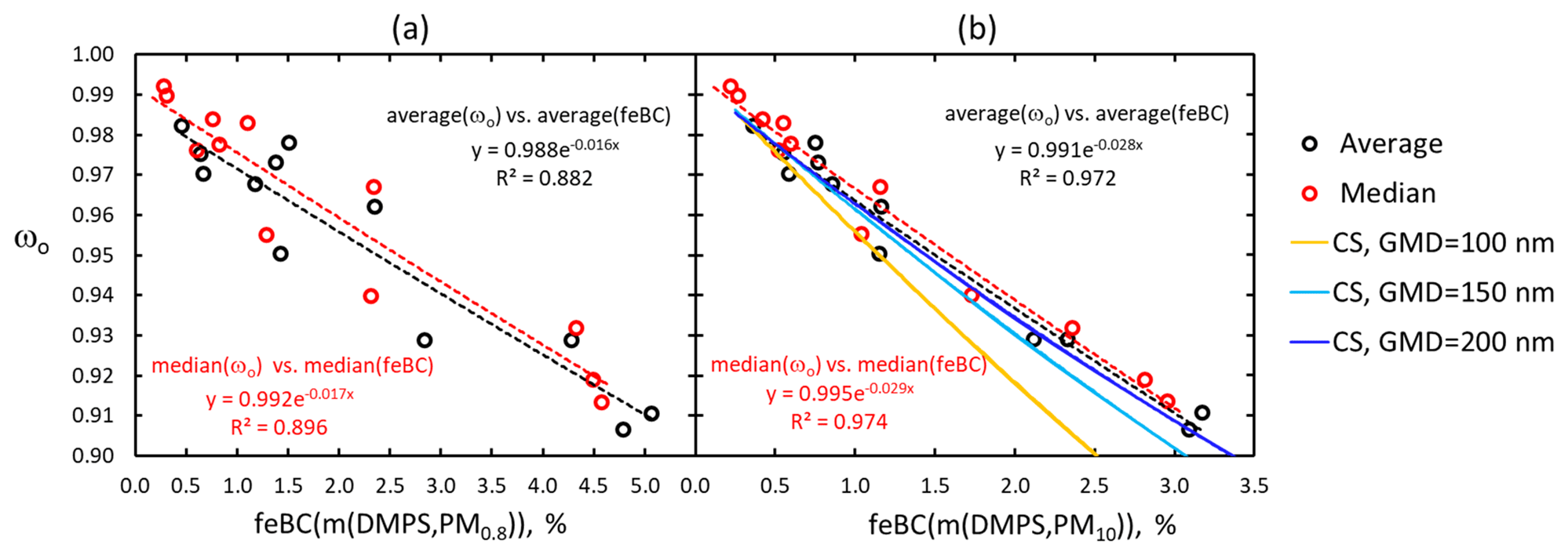
Figure 12 Monthly average and median ω_o vs. eBC mass fraction calculated as the ratio of eBC to (a) m(DMPS,PM_0.8) and (b) m(DMPS,PM₁₀). The dashed lines represent fittings of ${\mathit{\omega }}_{\text{o}}\left(f\text{eBC}\right)={\mathit{\omega }}_{\text{o}}\left(\mathrm{0}\right)\exp (-k\cdot f\text{eBC}$) with the data. The continuous lines in panel (b) represent simulations with a core-shell (CS) model for lognormal number size distributions with geometric standard deviation GSD = 1.8 and geometric mean diameter (GMD) shown in the legend.

To evaluate whether these relationships could be explained by coated spherical BC particles, lognormal size distributions n(D_p, GMD, GSD) were generated where GMD is the geometric mean diameter, GSD is the geometric standard deviation, and the D_p range is 3 nm–10 µm. In the simulations all particles had a BC core and a scattering shell, and the core volume fraction was the same for all particles in the size distribution. The core-shell model N-Mie (Voshchinnikov and Mathis, 1999) that is based on a recursive algorithm of Wu and Wang (1991) was used for calculating scattering and absorption efficiencies Q_s and Q_a and scattering and absorption coefficients. See Virkkula (2021) for a detailed description of the simulations.

The BC core volume fraction varied from 0.25 % to 4 % to cover the range of feBC(m(DMPS,PM₁₀)) shown in Fig. 12b. The simulated ω_o vs. feBC(PM₁₀) agrees best with the observation-derived values when GSD = 1.8 and GMD = 200 nm. Smaller GMD and GSD yield lower ω_o vs. feBC(PM₁₀). A rigorous error-minimizing procedure was not done since the main goal of this simulation was to show that core-shell geometry can explain the observed ω_o vs. feBC(PM₁₀) relationship. However, a deeper analysis of the modal structure of the size distributions was considered to be beyond the scope of the present paper. Note that it was not assumed above that all particles observed at Dome C had a BC core. The simulations did not use any of the measured number concentrations or absorption coefficients. They were pure simulations with generated size distributions and variable BC core and scattering shell volume fractions. They were conducted to study whether the observed ω_o vs. feBC(PM₁₀) relationship could be explained with size distributions of coated BC particles. However, considering that the BC particles observed at Dome C most probably have been transported from the surrounding continents for thousands of kilometers, it is very likely that most of the observed BC particles have been coated during aging processes.

3.4 Aerosol sources and transport and their seasonal cycles

Source areas were modeled by using FLEXPART as described in Sect. 2.7. The 60 000 50 d back trajectories were used for estimating vertical transport routes and the source areas of the observed aerosols. Sources of individual plumes are not analyzed: the main goal is to find explanations for the observed seasonal cycles of aerosol optical properties.

3.4.1 Vertical and horizontal transport

The average residence time of the trajectories in each grid cell in the altitude range 50–14 400 m a.g.l. south of the Equator is shown for the inert tracer and for the simulated BC aerosol tracer (Fig. 13). The average altitude of both the inert tracer and the BC tracer decreases sharply as the latitude approaches 75^∘ S, which shows that on average air masses descend over the high plateau. This is in line with several studies that show that stratospheric air is brought down into the lower troposphere by descending air masses above the Antarctic continent (Ito, 1989; James, 1989; Parish and Bromwich, 1991; King and Turner, 1997; Krinner and Genthon, 2003; Stohl and Sodemann, 2010). Even though the average altitude of the trajectories shows descending air masses above to Dome C for the inert tracer, the low-level residence times are high also at low levels (<1000 m a.g.l.) at latitudes south of about 40^∘ S, indicating that it is not uncommon that air masses flow near the surface up to Dome C.

When transport was modeled with FLEXPART using in-cloud and below-cloud scavenging of aged BC particles as described by Grythe et al. (2017), for the BC tracer the residence times are lower than for the inert tracer except near Dome C. Additionally, the average trajectory altitude is clearly different than for the inert tracer. Far from Antarctica the BC tracer residence times are clearly smaller than for the inert tracer. This is due to the removal of BC particles by in-cloud and below-cloud scavenging and dry deposition. As a result there would be essentially no BC particles arriving at Dome C from north of latitude 10^∘ S at altitudes <1600 m, which is indicated by the respective area in Fig. 13b as just white. Consequently, those BC particles that do get lifted above the clouds increase the average altitude of the BC tracer back trajectories compared with the inert tracer average altitude, as is shown by the respective black and white lines in Fig. 13b. At latitudes ∼20–50^∘ S the BC tracer average altitude is approximately 1000 m higher than that of the inert tracer.

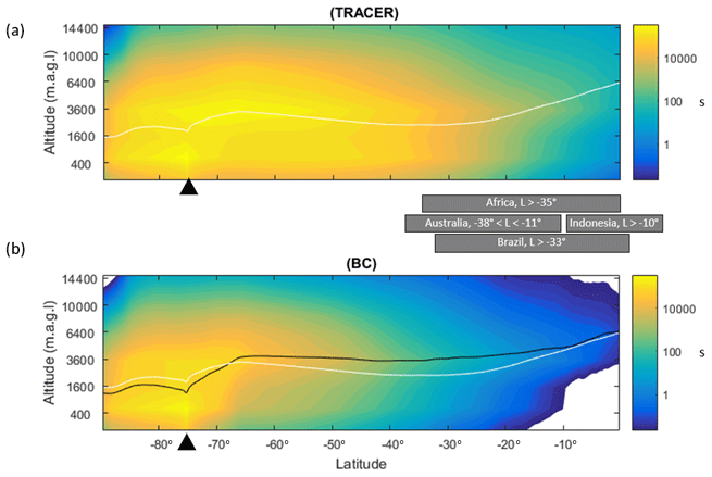
Figure 13 The residence time of 60 000 50 d FLEXPART back trajectories arriving at Dome C in 2008–2013 as a function of latitude and altitude above ground level. The residence time is color-coded from blue to yellow to show increasing time spent in each grid cell. (a) The residence times of the inert tracer back trajectories. White line: the average altitude of trajectories at each latitude. (b) Same as in panel (a) but for the BC tracer. Black line: the average altitude of the BC tracer; the white line is for comparison average altitude of the inert tracer. The black triangle shows the latitude of Dome C (75^∘06^′ S). The grey text boxes between (a) and (b) show the approximate latitude range of some major BC-emitting regions.

Between Fig. 13a and b there are grey text boxes that show the approximate latitude range of some major BC-emitting regions. Indonesia is north of 10^∘ S, so BC particles should rise to about 2 km altitude in order to get transported to Dome C. The Indonesian smoke plumes are generally lower than that (Tosca et al., 2011), so their contribution to eBC observed at Dome C is probably negligible. The other three main biomass-burning regions Africa, Australia, and Brazil are more to the south, and the smoke plume heights have been observed at clearly higher altitudes (Pereira et al., 2016; Rémy et al., 2017; Gonzalez-Alonso et al., 2019). Smoke plumes were recently observed at a height of 4 km over Brazil and even higher, at 6 km over Australia (Shikwambana and Kganyago, 2021). Comparison with Fig. 13b shows that from these altitudes it is likely that BC particles also reach Dome C. All this is in agreement with Fiebig et al. (2009), who established a source–receptor relationship between biomass-burning events in central Brazil and the aerosol observed at the Norwegian station Troll.

Near Dome C and over all continental Antarctica the BC tracer average altitude is lower than that of the inert tracer. When BC has a lower average altitude than the tracer, it means that the air at that point has undergone more removal above than below the average altitude. This suggests that near Dome C most removal takes place in the clouds, higher up than the release point. This implies that there is more in-cloud removal than precipitation scavenging or dry deposition over the plateau.

3.4.2 Source areas of eBC and high and low ω_o using footprint differences

Source areas were next estimated by using FLEXPART and calculating the footprint differences as described in Sect. 2.7.1. The relative difference (RD) (Eq. 19) of the emission sensitivities in the two lowest layers (<1000 m a.g.l.) was calculated for the highest and lowest 10 % of eBC concentration and ω_o. As was shown in Sect. 3.3, the highest and lowest ω_o percentiles correspond to the lowest and highest eBC mass fraction percentiles.

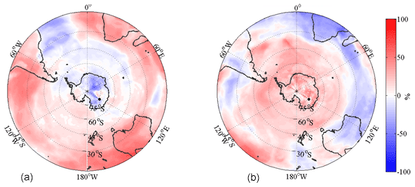
Figure 14 The relative difference, RD, Eq. (19), of transport for the two lowest layers (>1000 m a.g.l.) between the highest and lowest 10 % of (a) eBC concentration and (b) single-scattering albedo. Positive values indicate a relative increase in transport and negative values a decreased transport from a given area by the highest 10 % of measurements.

The highest eBC concentrations have an increased signal from the surrounding continents Australia, Africa, and South America (Fig. 14a). However, high RD values are also associated with large areas over the Pacific Ocean, the Indian Ocean, and the Atlantic Ocean. These high RD values on the oceans may in principle be due to shipping emissions, but it is more likely that they are due to BC emissions from the continents where the emissions are considerably higher than from shipping. Smoke from South America is predominantly transported southeast into the South Atlantic (Freitas et al., 2005; Reid et al., 2009; Ulke et al., 2011) and further to the east. African smoke first gets transported westward to the Atlantic Ocean by easterly winds (Reid et al., 2009). Most of this smoke wraps around the South Atlantic Subtropical High, gets mixed with the South American smoke plume, and flows east in the subtropical jet region towards Australia and even further to the remote South Pacific (Singh et al., 2000; Staudt et al., 2002; Chatfield et al., 2002). During the transport to higher latitudes, the smoke typically rises to about 5–7 km (Singh et al., 2000; Staudt et al., 2002; Reid et al., 2009).

In addition to the eastward transport in the subtropical jet smoke outflow associated with the trade winds, the dominating easterlies from South America towards the west to the Pacific Ocean have been observed between the Equator and 20^∘ S (Freitas et al., 2005; Ulke et al., 2011; Bourgeois et al., 2015). Bourgeois et al. (2015) studied aerosol transport over the Andes from the Amazon Basin to the remote Pacific Ocean by using 6 years (2007–2012) of data from the CALIOP satellite instrument. They found that mainly biomass-burning particles emitted during the dry season in the Amazon Basin are lifted in significant amounts over the Andes. Aerosols reaching the top of the Andes, at altitudes typically between 4 and 5 km, are entrained into the free troposphere (FT) over the southeastern Pacific Ocean, and they can be traced on average over 4000 km away from the continent, indicating an aerosol residence time of 8–9 d in the FT over the Pacific Ocean.

Koch et al. (2009) evaluated BC model predictions of several global models from the AeroCom model intercomparison project. Among several results they presented global maps of modeled BC surface concentrations and annual mean column BC loads predicted by the different models. Figure 14a displays similarities to both the measurement studies and the global model intercomparison results of Koch et al. (2009). Especially the global maps of annual mean column BC load for GISS sensitivity simulations (Fig. 8 of Koch et al., 2009) have several patterns that are similar to the relative difference RD calculated using Eq. (19) for eBC concentrations measured at Dome C. Here the features of these two figures are compared qualitatively by moving eastwards starting from Africa. The RD in Fig. 14a is high above Africa and in the Atlantic Ocean west of Africa, in agreement with the column BC load predicted by all the GISS sensitivity simulations. To the east, between Africa and Australia, there is a belt of high RD values, similar to most of the GISS sensitivity simulations. It is interesting that there is even a local minimum over the Indian Ocean in both the RD values and the GISS simulations. The values over Australia are also high in both figures. There is a clear difference east of Australia: the RD values are high even at the meridian of about 160–180^∘ W, although the BC load in most of the GISS simulations decreases clearly immediately to the east of Australia. The RD values then decrease to another local minimum at the meridian of about 150^∘ W and then increase towards South America, in agreement with the GISS sensitivity simulations. Over South America the RD values are positive but decrease to negative values in the South Atlantic immediately to the east of the continent. Such a decrease is not in the GISS sensitivity simulations. So, the RD values over the western half of the South Atlantic are the most suspicious ones in Fig. 14a. They suggest that the lowest eBC concentrations observed at Dome C were associated with air masses from there. This is not reasonable since the studies cited above show that South American smoke plumes generally flow to the South Atlantic. This discrepancy remains unexplained.

The highest ω_o are obviously related to SSA and biogenic secondary aerosol emissions from the Southern Ocean (Fig. 14b). The differences between the oceanic sectors are not big, but there are some: in the Atlantic and Pacific sectors the RD of ω_o is clearly positive south of latitude 30^∘ S, but in the Indian Ocean sector RD is positive south of latitude ∼40^∘ S. This can be compared with the chlorophyll-a (Chl-a) concentrations in five oceanic sectors presented by Becagli et al. (2021). They determined the seasonal cycle of Chl-a concentrations in five sectors: Weddell Sea (WS, 60^∘ W–20^∘ E), Indian Ocean (IO, 20–90^∘ E), western Pacific Ocean (WP, 90–160^∘ E), Ross Sea (RS, 160–130^∘ W), and the combined Bellingshausen and Amundsen seas (BA, 130–60^∘ W). They found that the highest Chl-a concentrations were in the WS, RS, and BA sectors and the lowest ones in the IO and WP sectors. This is in line with the above-described geographical distribution of the RD of ω_o in Fig. 14b, suggesting that the differences in the RD distributions are due to biogenic aerosols.

3.4.3 Seasonal cycles of air-mass transport from different regions

Seasonal cycles of meteorological processes and conditions also affect properties of aerosols observed at Dome C. The most evident is solar radiation that affects new particle formation (e.g., Ito, 1989; Fiebig et al., 2014; Järvinen et al., 2013), but important are also the seasonal cycles of transport from the surrounding continents and from the marine boundary layer of the Southern Ocean (Stohl and Sodemann, 2010). The seasonal contributions of air masses from different regions were calculated as the fraction of time the FLEXPART trajectories spent over Antarctica and the surrounding oceans and continents (Fig. 15).

Figure 15 Seasonal air-mass transport by region calculated as the fraction of time the FLEXPART 50 d trajectories spent over Antarctica and the surrounding oceans and continents.

In the austral summer (DJF) the contribution of continental air other than Antarctica is low, and its minimum is in April. This is also true for marine air masses other than the Southern Ocean. In summer the contribution of Antarctic air is at its highest. Then in May the air-mass transport from other continents increases clearly, and it reaches a maximum in July, a smaller fraction in August, and a second maximum in September. The seasonal cycle of transport from all the surrounding continental areas is qualitatively similar. It can be explained by the seasonal cycle of the tropospheric polar vortex. Waugh et al. (2017) described the structures, seasonality, and dynamics of the stratospheric and tropospheric polar vortices and their connections to extreme events at Earth's surface. Estimating from their Fig. 2, the approximate edge of the tropospheric polar vortex of the Southern Hemisphere is at the latitudes of 50^∘ S in January and 30^∘ S in July. This means that in the austral winter the southern parts of South America, Africa, and Australia are within the tropospheric polar vortex but not in the austral summer. This is in line with Fig. 15. The next question is how well the seasonal cycles of the aerosol optical properties observed at Dome C follow the emissions of major absorbing and scattering aerosols in different regions.

3.4.4 Relationships of seasonal cycles of BC emissions in the surrounding continents and eBC at Dome C

Monthly BC emissions from wildfires and agricultural burning and other fires in South America, Africa, and Oceania (Australia, New Zealand, Melanesia, Micronesia, and Polynesia) in 2006–2012 were downloaded from GFED v3.1. The seasonal cycles are presented in Fig. 16a together with the monthly average eBC concentrations – corrected for scattering – observed at Dome C. It is obvious in Fig. 16a that the maximum of the sum of the emissions occurs 3 months earlier than the maximum eBC concentration at Dome C.

The seasonal cycles of air mass residence time over each of the major source areas play a crucial role in explaining the relationship between eBC at Dome C and BC emissions. The BC emissions were multiplied by the fraction of the time (f(t)) the FLEXPART trajectories spent over each of the three major source areas shown in Fig. 15. These quantities (f(t)×BC emissions) will be called residence-time-weighted BC emissions, RTW BC emissions. They are plotted in Fig. 16b together with the normalized eBC concentrations. Linear regressions between the eBC concentration and RTW BC emissions were calculated, but only the respective squared correlation coefficients R² are shown. The correlation between eBC concentrations and RTW BC emissions is weak, R²<0.3 (Fig. 16b). However, the main reason is that the residence times shown in Fig. 15 present the fraction of time that trajectories arriving at Dome C at any given month have spent over each of the regions before arrival at Dome C. So, next it was assumed that the transport time from each of the source areas to Dome C is 1 month, so f(t) of each month was multiplied by the BC emission 1 month earlier. This shifts the RTW BC emission peaks of all the source areas so that all R² increase somewhat (Fig. 16c). When it is assumed that the transport time is 2 months, R² increase clearly, 0.688 for Oceania and 0.665 for South America, and for Africa correlation still remains low (Fig. 16d). In October–November, when the eBC concentrations at Dome C are the largest, the 2-month-shifted RTW BC emissions from South America are approximately an order of magnitude larger than from Africa and Oceania, suggesting that South American BC emissions are the largest contributor to eBC at Dome C.

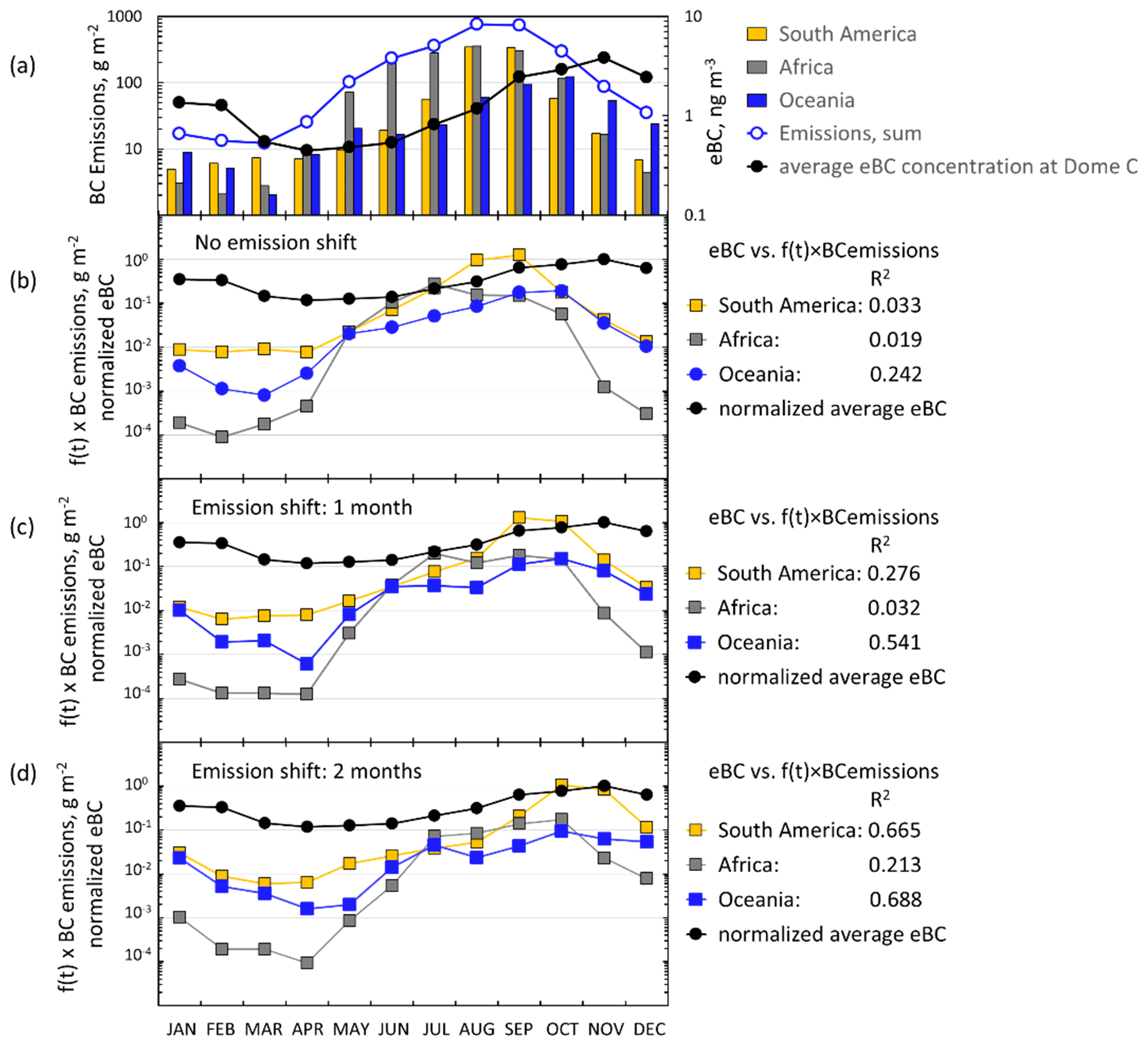
Figure 16 Seasonal cycles of fire-related BC emissions from the surrounding continents and eBC concentration at Dome C. (a) BC emissions and eBC concentrations, (b) RTW BC emissions, (c) f(t)×BC emissions 1 month earlier, and (d) f(t)×BC emissions 2 months earlier. The numbers show the squared correlation coefficient of linear regression between eBC concentrations and f(t)×BC emissions with the shown time shifts.

The highest correlation between the eBC concentrations and RTW BC emissions with the 2-month time shift suggests further that transport time is considerably longer than the 30 d Stohl and Sodemann (2010) obtained in a 5.5-year climatology of atmospheric transport into the Antarctic troposphere. The 2-month transport time naturally implies that BC aerosol residence time is also so long. Williams et al. (2002) estimated by modeling that in the upper atmosphere aerosols of 0.065 µm in size have residence times of approximately 1 month and can be transported on a hemispheric scale. Papastefanou (2006) determined residence times of tropospheric aerosols with different methods and obtained a much shorter mean value of 8 d. Kristiansen et al. (2012) estimated accumulation-mode aerosol removal times from the atmosphere using a global measurement data set collected over several months after the accident at the Fukushima Dai-ichi nuclear power plant in March 2011. After correction for radioactive decay, the ${}^{\mathrm{137}}\mathrm{Cs}{/}^{\mathrm{133}}\mathrm{Xe}$ ratios can be assumed to reflect the removal of aerosols by wet and dry deposition. Using this method, Kristiansen et al. (2012) obtained removal times for ¹³⁷Cs of 10.0–13.9 d. The simulations of Croft et al. (2014) with instantaneous injections into layers at 5 and 7 km yielded mean lifetimes of 14.7 and 21.1 d, respectively. At higher altitudes removal mechanisms are weaker, so lifetimes are longer. These are altitudes where biomass-burning smoke plumes have been observed, as discussed above. Note that these lifetimes are the e-folding lifetimes τ from $C\left(t\right)=C\left(t_{\mathrm{0}}\right)\exp (-t/\mathit{\tau })$. That means, for example, that if biomass-burning smoke where BC concentration is 1000 ng m⁻³ – similar to concentrations observed in a Brazilian biomass-burning measurement campaign (Brito et al., 2014) – rises to 5 km and gets transported for 60 d, the BC concentration decreases to 16.9 ng m⁻³. With τ=10 d the concentration would decrease to 2.5 ng m⁻³. At Dome C the 25th to 75th percentile range of eBC concentration in November is $\sim \mathrm{2}-\mathrm{6}$ ng m⁻³ (Table S7). As the simple estimation shows, this range is consistent with BC emissions of about 1 µg m⁻³ and transport for 2 months.

The above discussion does not mean that pollution episodes from the surrounding continents could not be transported more quickly than in 2 months. For instance, Fiebig et al. (2009) calculated the source areas and transport routes of an elevated aerosol concentration event observed at the Norwegian Troll station in Queen Maud Land. The analysis showed that the origin of the aerosol was biomass burning in Brazil 11–12 d before the arrival at Troll. Hara et al. (2010) analyzed several haze events observed at Syowa, the Japanese Antarctic coastal station. They found that the traveling time from southern Africa to Syowa varied in the range of 4 to 8 d, even more quickly than to Troll in the episode analyzed by Fiebig et al. (2009). The explanation for the considerably longer transport time to Dome C, 2 months, is that it was obtained from the correlation of seasonal cycles of BC emissions and observed concentrations, so it is more like a statistical estimate of seasonal transport times. That suggests that on average the BC emitted in the biomass burning in the surrounding continents circulates the Southern Hemisphere and migrates slowly towards the Antarctic upper plateau.

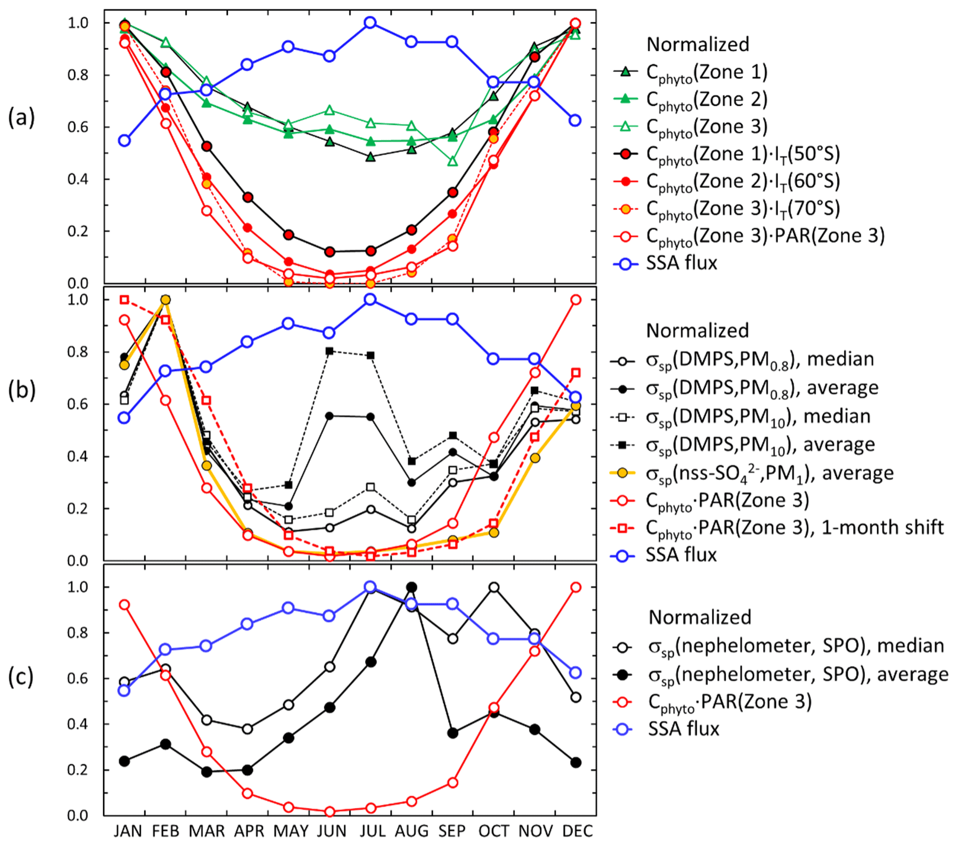
Figure 17 Normalized seasonal cycles of (a) major natural sources of light-scattering aerosols from the oceans, (b) scattering coefficients at Dome C, and (c) scattering coefficients at the SPO. σ_sp(DMPS,PM_0.8) and σ_sp(DMPS,PM₁₀): scattering coefficient calculated from particle number size distributions; σ_sp(nssSO${}_{\mathrm{4}}^{\mathrm{2}-}$,PM₁): scattering coefficient calculated from non-sea-salt sulfate concentrations in PM₁ filter samples; σ_sp(nephelometer, SPO): scattering coefficient measured with the nephelometer at the SPO; C_phyto: phytoplankton biomass concentration in 2008–2013 calculated as monthly averages from the time series presented by Behrenfeld et al. (2016) using CALIOP satellite data in Zone 1 (45–55^∘ S), Zone 2 (−65^∘ S), and Zone 3 (65–75^∘ S); I_T(50^∘ S), I_T(60^∘ S), and I_T(70^∘ S): average global radiation at latitudes 50, 60, and 70^∘ S at longitude 0^∘ at 10:00–14:00 UTC; PAR (Zone 3): photosynthetically active radiation from Behrenfeld et al. (2016); SSA: sea-spray aerosol flux modeled according to Grythe et al. (2014).

Figure 16 also shows that the observed concentration varies by an order of magnitude only, although the emissions vary by 2 orders of magnitude. This suggests that at the observed seasonal minimum eBC in March–April the sources are something else than wildfires and agricultural burning BC emissions in the GFED data. Possible sources can be other anthropogenic emissions, such as traffic including shipping, industrial emissions, and heating. Stohl and Sodemann (2010) estimated that ship emissions south of 60^∘ S account for half of the total BC concentrations in the lowest 1000 m of the atmosphere south of 70^∘ S in December. However, due to the particle removal processes as described in Sect. 3.4.1, the contributions of ship emissions to BC at Dome C are much lower. No quantitative estimations were calculated. Xu et al. (2021) recently presented a new global BC emission inventory for all countries in the world for the years 1960–2017. In an Excel file supplement, Xu et al. (2021) present the emissions classified into energy sector, industrial, residential, on-road motor vehicles, other anthropogenic, and wildfires. The sums of South American, Southern Hemisphere African, and Oceanian emissions in the period 2008–2013 and the respective contributions of wildfire emissions were calculated. They were $\sim \mathrm{40}\pm \mathrm{8}$ %, $\sim \mathrm{49}\pm \mathrm{2}$ %, and $\sim \mathrm{59}\pm \mathrm{9}$ % for South American, Southern Hemisphere African, and Oceanian emissions, respectively. However, only wildfire-emitted BC-particles have the potential to rise high enough to avoid in-cloud or below-cloud scavenging during the transport, as was discussed above.

3.4.5 Relationships of seasonal cycles of scattering aerosol emissions and σ_sp at Dome C and the SPO

The seasonal cycles of scattering coefficient at Dome C and at the SPO were compared with the seasonal cycles of secondary and primary marine aerosol emissions. The SSA emissions calculated with the FLEX-SSA offline tool (Sect. 2.7.2) show that SSA emissions from the Southern Ocean peak in the austral winter (Fig. 17a). Sea ice and the glacier surfaces, especially in the coastal regions, are also important sources of sea-salt aerosols (e.g., Frey et al., 2020; Hara et al., 2020). However, the aim was to find a qualitative explanation for the high scattering coefficients observed in winter, especially at the SPO. The FLEX-SSA offline tool was used for that, and it yields a seasonal cycle that at least partially explains the observations. There was no tool for estimating seasonal cycles of sea-salt emissions from sea ice.

Secondary marine aerosols are formed from the oxidation of emission products of phytoplankton. Becagli et al. (2021) discussed the relationships between biogenic aerosols (nssSO${}_{\mathrm{4}}^{\mathrm{2}-}$ and MSA⁻), chlorophyll-a concentration, which is a proxy for phytoplankton, sea ice extent and area, source areas, and the transport routes to Dome C and the Southern Annular Mode (SAM). They showed that these relationships are different in early, middle, and late austral summer. Here a subset of the data is analyzed in a method that is complementary to that of Becagli et al. (2021). The phytoplankton concentration maximum is in summer and the minimum in winter in the satellite data analysis of Behrenfeld et al. (2016) (Fig. 17a). However, phytoplankton concentration alone does not explain the seasonal cycle of secondary aerosol scattering coefficients. The DMS oxidation is a photochemical process, so a simplified method was used for estimating solar radiation intensity. Global radiation intensity I_T (W m⁻²) was calculated by using a clear-sky model for direct and diffuse insolation (Bird and Hulstrom, 1981). I_T was calculated at the surface (p=1000 mbar) for each hour of the year at the prime meridian (0^∘) at three latitudes, 50, 60, and 70^∘ S, corresponding to the central latitudes of Zone 1 (45–55^∘ S), Zone 2 (55–65^∘ S), and the polar zone, Zone 3 (65–75^∘ S). The monthly averages of I_T at 10:00–14:00 on each day of a month were calculated. The reasoning for using this time is that new particle formation is typically, although not exclusively, a daytime phenomenon at numerous locations around the world, also in Antarctica (e.g., Weller et al., 2015; Kerminen et al., 2018; Kim et al., 2019; Brean et al., 2021). The monthly product, C_phytoI_T, was then used as a proxy of biogenic secondary aerosol emissions. Behrenfeld et al. (2016) also presented the photosynthetically active radiation (PAR) in the polar zone obtained from the MODIS Aqua ocean color sensor acquired from http://oceancolor.gsfc.nasa.gov/cms (last access: 10 April 2022). In addition to the product C_phytoI_T, the monthly product C_phytoPAR was also calculated for Zone 3 and used as a proxy for biogenic secondary aerosol emissions. In Zone 3 the two emission proxies C_phytoI_T and C_phytoPAR agree well (Fig. 17a).

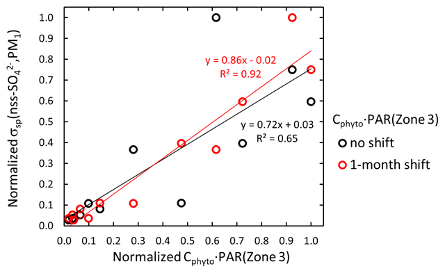
Figure 18 Normalized monthly average scattering coefficients calculated from the nss sulfate concentrations of the PM₁ filter samples σ_sp(nssSO${}_{\mathrm{4}}^{\mathrm{2}-}$,PM₁) at Dome C vs. normalized monthly averages of C_phytoPAR in the polar latitude zone with and without a time shift.

The normalized seasonal cycles of the SSA flux and the secondary aerosol emission proxy C_phytoPAR in the polar zone are plotted together with the normalized seasonal cycles of the scattering coefficients at Dome C (Fig. 17b) and at the SPO (Fig. 17c). At Dome C both σ_sp(DMPS,PM_0.8) and σ_sp(DMPS,PM₁₀) approximately follow the seasonal cycle of the secondary aerosol emissions in October–April. In the austral winter the effect of SSA is visible, especially in the high monthly σ_sp averages. The medians are clearly lower, and they follow the secondary aerosol emission proxy even in May. Also, the normalized seasonal cycle of σ_sp(nssSO${}_{\mathrm{4}}^{\mathrm{2}-}$,PM₁), the scattering coefficient calculated from non-sea-salt sulfate concentrations in PM₁ filter samples, is presented in Fig. 17b. It also follows approximately the seasonal cycle of C_phytoPAR for the whole year. However, there appears to be a time lag. C_phytoPAR grows quickly in October, but σ_sp(nssSO${}_{\mathrm{4}}^{\mathrm{2}-}$,PM₁) in November. When C_phytoPAR is shifted by 1 month, they agree clearly better. The linear regression of σ_sp(nssSO${}_{\mathrm{4}}^{\mathrm{2}-}$,PM₁) vs. C_phytoPAR yields the correlation coefficient R²=0.65 when there is no C_phytoPAR time shift and R²=0.92 when C_phytoPAR is shifted by 1 month (Fig. 18). This suggests that on average it takes approximately a month for the secondary aerosol to be formed, grown, get mixed in the upper atmospheric layers, and be transported to the upper plateau. As was discussed above, Williams et al. (2002) estimated by modeling that in the upper atmosphere aerosol residence time can be ∼1 month, and Croft et al. (2014) obtained e-folding lifetimes of ∼15 and ∼21 d at 5 and 7 km altitudes, respectively, so it is reasonable.

There is one thing that the time shift cannot explain. The maximum σ_sp – and mass concentrations as discussed in Sect. 3.3 – was in February. This cannot be explained by the seasonal cycle of the biogenic secondary aerosol emission proxy: the maximum C_phytoPAR was in December, so even a 1-month transport time does not make February the maximum. Above it was assumed that the proxy is simply the product C_phytoPAR. However, the underlying hypothesis of this proxy is that the emissions of the precursor gases of new particle formation, mainly DMS, are linearly related to the phytoplankton mass concentrations. This is probably not the case, and there are other factors. Another explanation could be meteorological. Becagli et al. (2021) showed that the MSA and nssSO${}_{\mathrm{4}}^{\mathrm{2}-}$ maxima in February could possibly be explained by faster transport from the surrounding oceans with air masses traveling at lower elevation than in December–January. Further analyses of that relationship are out of the scope of the present paper, however. For more details, see Becagli et al. (2021). Note that σ_sp(nssSO${}_{\mathrm{4}}^{\mathrm{2}-}$, PM₁) correlates well also with C_phytoI_T of zones 1 and 2 shown in Fig. 17a, which means the secondary marine aerosol may have been formed and grown also further to the north than in the polar zone.

At the SPO, σ_sp is more strongly affected by the SSA emissions than at Dome C, especially in the austral winter and spring (Fig. 17c). Note that at the SPO the seasonal cycle of the normalized median σ_sp follows roughly the normalized SSA emission flux in July–December. The seasonal cycle of the normalized average σ_sp is different because averages are affected more by individual high transport events and medians represent better the prevailing background aerosol of the season. As explained above, the difference between Dome C and the SPO may either be due to geographical locations, different size ranges measured by the instruments, or both.

4 Summary and conclusions

Aerosol optical properties have been measured at several Antarctic sites, but scattering and absorption data measured at Dome C were not examined in detail earlier. This work fills that gap using light absorption from a 3λ PSAP and light-scattering coefficients (σ_sp) calculated from particle number size distributions measured with a differential mobility particle sizer (DMPS) and an optical particle counter (OPC). Additionally, single-scattering albedo (ω_o), absorption Ångström exponent (α_ap), scattering Ångström exponent (α_sp), and equivalent black carbon (eBC) concentrations were calculated. The sources of the aerosol were estimated by calculating footprints with FLEXPART and by calculating seasonal cycles of transport of both scattering and absorbing particles from different source areas.

Aerosol light-scattering coefficients were calculated from the DMPS size distributions using two different refractive indices and the contribution of scattering due to particles larger than those measured with the DMPS to provide a lower and an upper estimate of σ_sp. Light scattering was also estimated using mass scattering efficiencies in conjunction with mass concentrations obtained from PM₁ and PM₁₀ filter samples. The two most frequently used algorithms to calculate aerosol absorption coefficients (σ_ap) from PSAP measurements require scattering coefficients. Both algorithms were applied and both the upper and lower estimates of σ_sp were used in order to provide understanding of the differences between the algorithms and the impact of the scattering adjustment. The absorption coefficient calculated using the σ_sp upper estimate was considered to be the best σ_ap estimate.

There were clear seasonal cycles of σ_sp and σ_ap at Dome C. The maximum and minimum of σ_sp were observed in austral summer and winter, respectively. The Dome C scattering coefficients were also compared with σ_sp measured with a nephelometer at the South Pole Station (SPO). At the SPO the scattering coefficient was similar to that measured at Dome C in austral summer, but there was a large difference in the austral winter. At the SPO the maximum monthly averages were observed in austral winter. This suggests that, in winter, the SPO is more influenced by sea-spray emissions than Dome C. At Dome C the σ_ap exhibited a different seasonal cycle of than σ_sp – the minimum σ_ap was observed in the austral autumn and the maximum in spring. As a result, the seasonal cycle of the single-scattering albedo ω_o is such that the darkest aerosol, i.e., the lowest ω_o≈0.91, is observed in October and the highest ω_o>0.99 in February and March.

The scattering Ångström exponent α_sp calculated from the σ_sp lower estimate varied from ∼2.6 in austral summer to ∼2.1 in austral winter, indicating that in austral summer the size distributions are dominated by smaller particles than in winter. For the σ_sp upper estimate α_sp varied from ∼1.9 in austral summer to ∼0.8 in winter. This seasonal cycle is quite similar to the seasonal cycle of α_sp of σ_sp measured at the SPO. The uncertainty of the absorption Ångström exponent α_ap is high, particularly in the clean conditions existing in Antarctica. However, despite the high uncertainties the seasonal cycles of α_ap, with and without the scattering correction, are qualitatively similar: the lowest monthly medians are observed in March, while the maxima occur in August–October. This cycle – even that of the non-scattering-corrected α_ap – is anticorrelated with the ω_o seasonal cycle.

The eBC mass concentrations were compared with eBC measured at three other sites: the South Pole and two coastal sites Neumayer and Syowa. The maximum monthly median eBC concentrations are almost the same ($\sim \mathrm{3}\pm \mathrm{1}$ ng m⁻³) at all these sites in October–November. This suggests that, as far as eBC is concerned, there is no significant difference between the coastal and plateau sites. The seasonal cycle of eBC is slightly different from the mass concentration calculated from the number size distributions measured with the DMPS. Consequently, the seasonal cycle of the eBC mass fraction (f(eBC)) is such that f(eBC) minimum is in February–March and the maximum is in August–October, anticorrelating with ω_o. The eBC mass fractions in this peak are actually quite high and vary around 4 %–5 % with the 75th percentiles > 6 %–7 %, only slightly depending on PSAP correction algorithm. These levels of eBC mass fractions are typically observed in polluted air, suggesting that in these periods a large fraction of aerosol is long-range transported aerosol from other continents.

Source areas were calculated with 50 d FLEXPART footprints. The relative differences of the footprints calculated for the highest and lowest 10 % of eBC concentrations and ω_o showed that the highest eBC concentrations and the lowest ω_o were associated with air masses coming from South America, Australia, and Africa. Vertical simulations that take BC particle removal processes into account show that there would be essentially no BC particles arriving at Dome C from north of latitude 10^∘ S at altitudes <1600 m. The main biomass-burning regions Africa, Australia, and Brazil are more to the south, and their smoke plumes have been observed at higher altitudes than that, so they can get transported to Antarctica.

The seasonal cycle of BC emissions from wildfires and agricultural burning and other fires in South America, Africa, and Australia were calculated from data downloaded from the GFED. The maximum total emissions were in August–September, but the peak of monthly average eBC concentrations is observed in November, 2–3 months later, not only at Dome C, but also at the South Pole and the coastal stations. This is considerably longer than the 30 d presented in an earlier study. If this peak eBC concentration is really due to the peak emissions from the above-mentioned fires in the surrounding continents it means that the aerosol from these fires remains in air for several months and gets mixed essentially over the entire Southern Hemisphere. This does not mean that pollution episodes from the surrounding continents could not be transported faster than in 2 months. Earlier studies have clearly shown that biomass-burning smoke can get transported from South America or Africa to Antarctica in 1–2 weeks. The explanation for the considerably longer transport time to Dome C, 2 months, is that it was obtained from the correlation of seasonal cycles of BC emissions and observed concentrations, so it is more like a statistical estimate of seasonal transport times. That suggests that on average the BC emitted in the biomass burning in the surrounding continents circulates the Southern Hemisphere and migrates slowly towards the Antarctic upper plateau.

The seasonal contributions of air masses from different regions were calculated as the fraction of time the FLEXPART trajectories spent over Antarctica, the surrounding oceans and continents. The BC emissions were multiplied by the fraction of time the trajectories spent over each of the three major source areas. In October–November, when the eBC concentrations at Dome C are the largest the 2-month-shifted residence-time-weighted BC emissions from South America are approximately an order of magnitude larger than from Africa and Oceania, suggesting that South American BC emissions are the largest contributor to eBC at Dome C.

The seasonal cycles of scattering coefficient at Dome C and at the SPO were compared with the seasonal cycles of secondary and primary marine aerosol emissions. The seasonal cycles of SSA emissions were simulated with the FLEX-SSA offline tool. The seasonal cycles of biogenic secondary aerosols were estimated from monthly average phytoplankton biomass concentrations obtained from the CALIOP satellite sensor data. The correlation coefficients between scattering coefficients measured at Dome C and phytoplankton biomass concentrations and a biogenic secondary aerosol emission proxy are high. It may take a month for the biogenic aerosol to be formed and get transported from sea level to Dome C. The scattering coefficients measured at the SPO correlated much better with the SSA emission fluxes in the Southern Ocean than the scattering coefficients measured at Dome C. The difference between the scattering coefficients at these sites may either be due to geographical locations, different size ranges measured by the instruments or both.