Influence of photochemical loss of volatile organic compounds on understanding ozone formation mechanism

Volatile organic compounds (VOCs) tend to be consumed by atmospheric oxidants, resulting in substantial photochemical loss during transport. An observation-based model was used to evaluate the influence of photochemical loss of VOCs on the sensitivity regime and mechanisms of ozone formation. Our results showed that a VOC-limited regime based on observed VOC concentrations shifted to a transition regime with a photochemical initial concentration of VOCs (PIC-VOCs) in the morning. The net ozone formation rate was underestimated by 3 ppb h⁻¹ (∼36 ppb d⁻¹) based on the measured VOCs when compared with the PIC-VOCs. The relative contribution of the RO₂ path to ozone production based on the PIC-VOCs accordingly increased by 13.4 %; in particular, the contribution of alkene-derived RO₂ increased by approximately 10.2 %. In addition, the OH–HO₂ radical cycle was obviously accelerated by highly reactive alkenes after accounting for photochemical loss of VOCs. The contribution of local photochemistry might be underestimated for both local and regional ozone pollution if consumed VOCs are not accounted for, and policymaking on ozone pollution prevention should focus on VOCs with a high reactivity.

1 Introduction

Ground surface ozone (O₃) is an important atmospheric pollutant that is harmful to human health and is connected with respiratory, cardiovascular diseases, and premature mortality (Cohen et al., 2017). It is also harmful to vegetation growth. For example, it led to annual reductions in the yields of rice and wheat of 8 % and 6 %, respectively, and reduced forest biomass growth by 11 %–13 % in 2015 in China (Feng et al., 2019). Surface O₃ concentrations have increased by 11.9 % over eastern China despite the air pollution control measures implemented in China from 2012 to 2017 (Dang and Liao, 2019). An economic loss of 0.09 % of Chinese gross domestic product (CNY 78 billion) is predicted for 2030 if policies against O₃ pollution are not properly implemented (Xie et al., 2019). Therefore, urgent action to minimize O₃ pollution in China is needed.

Tropospheric O₃ is mainly produced from photochemical reactions between volatile organic compounds (VOCs) and nitrogen oxides (NO_x: NO+NO₂) (Seinfeld and Pandis, 2016; Liu et al., 2021). O₃ is generated from a collision of O₂ and O(3^P) that is produced from photolysis of NO₂ in the atmosphere. Peroxyl radicals (HO₂ and RO₂), which are produced from the oxidation of VOCs by the OH radical can efficiently convert NO (from the photolysis of NO₂) to NO₂, leading to a net O₃ production by compensating for the titration of O₃ by NO (Monks, 2005; Zhang et al., 2021a). Over the past 2 decades, a number of field observations focused on O₃ pollution levels, and its precursors have been carried out in the Beijing–Tianjin–Hebei (BTH), Yangtze River Delta (YRD), and Pearl River Delta (PRD) regions (Wang et al., 2017; Li et al., 2019; Xue et al., 2014; Zhang et al., 2019). Due to the nonlinear relationship between O₃ and its precursors and the variations in meteorological conditions, numerous studies have been performed to understand the sensitivity regime of O₃ formation (Ling and Guo, 2014; Zhang et al., 2020), the photochemical process of O₃ formation based on box models or observation-based models (OBMs) (He et al., 2019; Tan et al., 2019), and the sources of O₃ using regional chemical transport models (Li et al., 2016b, c). Recently, the instantaneous production rate of the O₃ formation process has attracted more attention; for example, studies examining radical recycling (OH–RO₂–RO–HO₂–OH) related to the production of O₃ have been performed (Lu et al., 2017; Tan et al., 2017; Whalley et al., 2018). HCHO photolysis and alkene ozonolysis contributed approximately 85 % to the primary production of HO₂ and HO radicals in Beijing, Shanghai and Guangzhou (Tan et al., 2019; Yang et al., 2017). The importance of HONO and HCHO photolysis for primary radical production has also been proposed in suburban and rural areas (Tan et al., 2017; Lu et al., 2012, 2013).

All of the OBM studies investigating the relationship between O₃ and VOCs were based on measured datasets. However, VOCs are highly reactive to atmospheric oxidants, such as OH, NO₃, and O₃, among which OH is dominant. The lifetimes of some highly reactive VOCs, such as isoprene, are as short as only a few tens of minutes under typical daytime atmospheric conditions. The mixing ratios of VOCs observed at a sampling site are actually the residues of VOCs from emissions due to the photochemical loss during transport from the source site to the receptor site. If photochemically consumed VOCs are not considered, the O₃ formation sensitivity and net O₃ production may be misunderstood, and subsequent policymaking on O₃ pollution prevention at regional or urban scales may be misguided. Thus, the photochemical age-based approach has been applied to evaluate the effect of photochemical processes on VOC measurements (Shao et al., 2011). This method was used to qualitatively or semi-quantitatively estimate the O₃ formation process of the source-receptor (Gao et al., 2018) by calculating the O₃ formation potential (OFP) (Han et al., 2017), identifying the critical species for O₃ formation (Gao et al., 2021), or evaluating the VOC emissions ratio (Yuan et al., 2013). In evaluating the importance of initial VOCs to ozone production, Xie et al. (2008) found that the OFP at a Peking University site increased by 70 % after accounting for the photochemical loss of VOCs. Li et al. (2015) also showed that the OFPs of total NMHCs (excluding isoprene) increased by 16.1 % (from 59.6 to 69.2 ppb O₃), 12.1 % (from 33.5 to 37.5 ppb O₃), and 3.4 % (from 68.9 to 71.2 ppb O₃) after correcting for photochemical loss in Gucheng, Quzhou, and Beijing, respectively. Gao et al. (2018) reported that the OFP could be underestimated by 23.4 % (62.4 ppb O₃) in Beijing if the photochemical loss of VOCs is not considered. Zhan et al. (2021) found that based on measured VOCs, the OFP increased from 57.8 to 103.9 ppb using the initial VOCs. All the previous work was based on the maximum incremental reactivities (MIR) method. The application of such calculations using the MIR method is restricted to areas or episodes in which O₃ formation is VOC sensitive (Carter, 1994). In the troposphere, the sensitivity of ozone formation to NO_x and VOCs varies greatly, as evidenced by the wide range of OFP underestimations from ∼3 % to 70 % in previous work. In addition, the MIR values of VOC species for a specific region are calculated with the base scenario, in which NO concentration and other parameters are the values that correspond to the maximal incremental reactivity (IR). The fixed MIR values of different VOCs can neither reflect the nonlinear relationship between ozone and VOCs, involved in the complicated radical recycling (OH–RO₂–RO–HO₂–OH) related to the production of ozone, nor be used for analyzing the radical budget of the initial VOCs concentration. Thus, a quantitative analysis is necessary to explicitly understand the influence of photochemical loss of VOCs on ozone formation and its mechanism based on OBM studies, in which the dynamic atmospheric and meteorological conditions is accounted for.

In this study, an OBM was used to evaluate the local O₃ formation process in summer in Beijing based on concentrations of observed and photochemical initial concentrations of VOCs (PIC-VOCs). The O₃–NO_x–VOC sensitivity, instantaneous O₃ formation rate, and in situ O₃ formation process were discussed. The aim of this study was to understand the possible influence of photochemical loss of VOCs on the formation sensitivity regime of O₃ and how the photochemical loss of VOCs affects O₃ formation. This study can provide new insight for better understanding atmospheric O₃ pollution.

2 Methodology

2.1 Experimental section

Field observations were carried out on the Qingyuan campus of the Beijing Institute of Petrochemical Technology (BIPT, 39.73^∘ N and 116.33^∘ E) (Fig. S1 in the Supplement). Details on the observation site have been described in our previous work (Zhan et al., 2021). In short, the site is a typical suburban site in the Daxing District between 5th Ring Road and 6th Ring Road. The field campaign was carried out during 1–28 August 2019, when photochemistry was the most active and rainfall was rare in Beijing.

The concentrations of non-methane hydrocarbons (NMHCs) were detected by both a gas chromatography–flame ionization detector (GC/FID) and a single photon ionization mass spectrometer (SPI-MS 3000, Guangzhou Hexin Instrument Co., Ltd., China). A detailed description of the instrumentation can be found in previous publications (Zhan et al., 2021; Chen et al., 2020). The SPI-MS was also used to detect halohydrocarbons. More details on this instrument and its parameter settings have been described in previous studies (Zhang et al., 2019; Liu et al., 2020a). In short, a 0.002 in. thick polydimethylsiloxane (PDMS) membrane (Technical Products Inc., USA) was used to collect VOCs and diffuse them from the sample site to the detector under high vacuum conditions. Vacuum ultraviolet (VUV) light generated by a commercial D2 lamp (Hamamatsu, Japan) was utilized for ionization at 10.8 eV. For ion detection, two microchannel plates (MCPs, Hamamatsu, Japan) assembled with a chevron-type configuration were employed. This TOF-MS has a limit of detection (LOD) varying from 50 to 1 ppb with a 1 min time resolution for most trace gases without any preconcentration procedure. To verify the data compatibility of the SPI-MS and GC/FID, we compared the concentrations of toluene measured using these two different instruments (Fig. S2). The correlation coefficient was 0.9 (with a slope of 0.7), indicating that the concentrations of NMHCs were comparable using these two measurement techniques.

Oxygenated VOCs (OVOCs) were collected using 2,4-dinitrophenylhydrazine (DNPH)-coated silica gel cartridges (Sep-Pak, Waters) by an automatic sampling device with a sampling flow rate of 1.2 L min⁻¹ and a duration of 2 h for each sample. Following this, the OVOCs were analyzed using high-performance liquid chromatography (HPLC, Inertsil ODS-P 5 µm 4.6×250 mm column, GL Sciences) with an acetonitrile–water binary mobile phase (Ma et al., 2019). To avoid possible contamination or desorption after sampling, cartridges were capped, placed into tightly closed plastic bags and kept in a refrigerator before analysis. The sampled cartridges were eluted with 5 mL acetonitrile and analyzed by HPLC as soon as possible after they were shipped back to the laboratory. This system was calibrated with eight-gradient standard solutions (TO11/IP-6A Aldehyde/Ketone-DNPH Mix, SUPELCO). The correlation coefficients were all greater than 0.999. The LOD for most OVOCs was approximately 10 ppt.

Trace gases, including NO_x, SO₂, CO, and O₃, were measured using corresponding analyzers (Thermo Scientific, 42i, 43i, 48i, and 49i, respectively). The HONO concentration was measured using a homemade long-path absorption photometer (LOPAP) (Liu et al., 2020c). The meteorological parameters, including temperature (T), pressure (P), relative humidity (RH), wind speed, and wind direction, were measured by a weather station (AWS310, Vaisala). The photolysis rate (JNO₂) was measured via continuous measurement of the actinic flux in the wavelength range of 285–375 nm using a JNO₂ filter radiometer (JNO₂ radiometer, Metcon).

2.2 Calculation of photochemical loss of VOCs

The photochemical loss of VOCs was calculated using the ratio method (Wiedinmyer et al., 2001; Yuan et al., 2013). The initial mixing ratio of a specific VOC was calculated using the following equations (Mckeen et al., 1996):

$$\begin{array}{}\text{(1)}& {\displaystyle }[{\mathrm{VOC}}_i{]}_{\mathrm{t}}=[{\mathrm{VOC}}_i{]}_{\mathrm{t}\mathrm{0}}\times \exp \left(-k_i\times \left[\mathrm{OH}\right]\times \mathrm{\Delta }t\right)\text{(2)}& {\displaystyle }\mathrm{\Delta }t={\displaystyle \frac{\mathrm{1}}{\left[\mathrm{OH}\right]\times \left(k_{\mathrm{X}}-k_{\mathrm{E}}\right)}}\times \left\{\ln \left({\displaystyle \frac{X_{\mathrm{0}}}{E_{\mathrm{0}}}}\right)-\ln \left({\displaystyle \frac{X_{\mathrm{t}}}{E_{\mathrm{t}}}}\right)\right\},\end{array}$$

where [VOC_i]_t and [VOC_i]_t0 are the observed and initial concentrations of VOC_i, respectively; k_i is the second-order reaction rate between compound i and OH radical; and [OH] and Δt are the concentration of OH radical and the photochemical aging time, respectively. k_E and k_X are rate constants for the reaction between OH radicals and ethylbenzene ($\mathrm{7.00}\times {\mathrm{10}}^{-\mathrm{12}}$ cm³ molec.⁻¹ s⁻¹) and xylene ($\mathrm{1.87}\times {\mathrm{10}}^{-\mathrm{11}}$ cm³ molec.⁻¹ s⁻¹) (Atkinson and Arey, 2003), respectively. ($X_{\mathrm{0}}/E_{\mathrm{0}})$ is the initial mixing ratio between xylene and ethylbenzene, and ($X_{\mathrm{t}}/E_{\mathrm{t}})$ is the mixing ratio between xylene and ethylbenzene at the observation time. In this study, we chose the mean concentrations of xylene and ethylbenzene at 05:00–06:00 LT as their initial concentrations before sunrise according to the ambient JNO₂ (Fig. S3) to calculate the photochemical loss of OH exposure. In previous work (Shao et al., 2011; Zhan et al., 2021), the selection of ethylbenzene and xylene as tracers was justified for calculating ambient OH exposure under the following conditions: (1) the concentrations of xylene and ethylbenzene were well correlated (Fig. S4), which indicated that they were simultaneously emitted; (2) they had different degradation rates in the atmosphere; and (3) the calculated PICs were in good agreement with those calculated using other tracers, such as i-butene/propene (Fig. S5) (Zhan et al., 2021). To test the relative constant emission ratio from different sources, we chose benzene vs. acetylene and n-hexane vs. toluene as references, and the result is shown in Fig. S6. These ambient ratios could directly reflect their relative emission rates from sources (Goldan et al., 2000; Jobson et al., 2004). The linear correlation coefficients (R²) were generally higher than 0.7, which were equal to that reported by Shao et al. (2011). To further test the assumption that the emissions of xylene and ethylbenzene were constant throughout the day, their potential sources were calculated using a source–receptor model (the potential source contribution function, PSCF). As shown in Fig. S7, xylene and ethylbenzene showed similar distributions. In addition, the ratio of $\mathrm{ethylbenzene}/\mathrm{xylene}$ at 05:00 and 06:00 LT was similar to that during the daytime. These results indicated that the emissions of xylene and ethylbenzene were constant throughout the day. The ratio of xylene to ethylbenzene and the OH exposure concentration are shown in Fig. S8. The results showed that the ratio of xylene to ethylbenzene increased gradually (07:00–12:00 LT), which is consistent with the trend of xylene and ethylbenzene. The OH exposure was from 0.82 to 8.1×10⁶ molec. cm⁻³ h, with a mean daytime value of $\mathrm{4.3}\pm \mathrm{1.9}\times {\mathrm{10}}^{\mathrm{6}}$ molec. cm⁻³ h. Accordingly, the mean photochemical ages were 1.7±0.9 h using the mean daytime (8:00–17:00 LT) OH concentrations ($\mathrm{4.3}\pm \mathrm{3.1}\times {\mathrm{10}}^{\mathrm{6}}$ molec. cm⁻³) calculated based on J(O¹D) using the method reported in our previous work (Liu et al., 2020b, 2020c). This meant that VOCs would undergo obvious degradation even during a short range of transport in the atmosphere.

It should be noted that the k_OH of isoprene is $\mathrm{9.98}\times {\mathrm{10}}^{-\mathrm{11}}$ cm³ molec.⁻¹ s⁻¹ at 298.15 K (Atkinson and Arey, 2003), almost 2 orders of magnitude greater than other VOCs. The ratio method assumes constant emissions for VOCs. However, the emission of isoprene greatly depends on temperature and solar irradiation intensity (Zhang et al., 2021b). In addition to accounting for photochemical loss, additional correction of daytime isoprene concentrations was performed using the average diurnal flux of isoprene emissions (Fig. S9; Zhang et al., 2021b). The emission of isoprene showed a clear unimodal curve, and the volume concentration of isoprene was calculated based on the daily emission curve using Eq. (S1) in the Supplement.

2.3 Observation-based model simulation

A box model based on the Master Chemical Mechanism (MCM3.3.1) and the Regional Atmospheric Chemical Mechanism (RACM2) was used in this study. The MCM3.3.1 was used to understand the instantaneous ozone formation process, and the RACM2 was used to depict the ozone isopleth due to its high computational efficiency (Sect. 2.4). Table S1 in the Supplement shows the model inputs. The model calculations were constrained with the measured meteorological parameters (RH, T, P, and JNO₂) and the concentrations of trace gases, including inorganic species (NO, NO₂, CO, SO₂, and HONO) and 61 organic species (NMHCs (46), OVOCs (8), and halohydrocarbons (7)). The model was validated using the observed and simulated O₃ concentrations, which showed good consistency, as shown in Fig. S10. The slope and correlation coefficients were 0.9 and 0.8, respectively (Fig. S11), indicating the validity of the model simulation. It is worth mentioning that the results of model simulation can sometimes be overestimated or underestimated to some extent, which has also been reported by previous studies (Zong et al., 2018; Zhang et al., 2020), but this did not affect our simulations of the ozone formation process and mechanisms because we constrained the ozone concentration during our simulations.

The ozone formation rate P(O₃) can be quantified by the oxidation rate of NO to NO₂ by peroxyl radicals (Tan et al., 2019), as expressed in Eq. (3). In this study, the modeled peroxyl radical concentrations were used to calculate the ozone production rate as follows

$$\begin{array}{}\text{(3)}& P\left({\mathrm{O}}_{\mathrm{3}}\right)=k_{{\mathrm{HO}}_{\mathrm{2}}+\mathrm{NO}}\left[{\mathrm{HO}}_{\mathrm{2}}\right]\left[\mathrm{NO}\right]+k_{{\mathrm{RO}}_{\mathrm{2}}+\mathrm{NO}}\left[{\mathrm{RO}}_{\mathrm{2}}\right]\left[\mathrm{NO}\right],\end{array}$$

where P(O₃) is the ozone formation rate, [HO₂] and [RO₂] are the number concentrations of HO₂ and RO₂ radicals, $k_{{\mathrm{HO}}_{\mathrm{2}}+\mathrm{NO}}$ is the second reaction rate between HO₂ and NO, and $k_{{\mathrm{RO}}_{\mathrm{2}}+\mathrm{NO}}$ is the second reaction rate for the reaction of RO₂ and NO, which only produces RO and NO₂. Once ozone forms, it will be consumed by OH, HO₂, and alkenes. Additionally, some NO₂ can react with OH, resulting in the formation of nitrate before photolysis. The chemical loss of both O₃ and NO₂ is considered in the calculation of the net ozone production rate (Tan et al., 2019),

$$\begin{array}{}\text{(4)}& \begin{array}{rl}L\left({\mathrm{O}}_{\mathrm{3}}\right)& =\left(k_{{\mathrm{O}}_{\mathrm{3}}+\mathrm{OH}}\left[\mathrm{OH}\right]+k_{{\mathrm{O}}_{\mathrm{3}}+{\mathrm{HO}}_{\mathrm{2}}}\left[{\mathrm{HO}}_{\mathrm{2}}\right]\right.\\ & \left.+k_{{\mathrm{O}}_{\mathrm{3}}+\mathrm{alkenes}}\left[\mathrm{alkenes}\right]\right)\left[{\mathrm{O}}_{\mathrm{3}}\right]\\ & +k_{{\mathrm{NO}}_{\mathrm{2}}+\mathrm{OH}}\left[{\mathrm{NO}}_{\mathrm{2}}\right]\left[\mathrm{OH}\right],\end{array}\end{array}$$

where L(O₃) is the ozone chemical loss rate; [OH] is the number concentration of OH radical; $k_{{\mathrm{O}}_{\mathrm{3}}+\mathrm{OH}}$, $k_{{\mathrm{O}}_{\mathrm{3}}+{\mathrm{HO}}_{\mathrm{2}}}$, and $k_{{\mathrm{O}}_{\mathrm{3}}+\mathrm{alkenes}}$ are the second-order reaction rate constants between O₃ and OH, HO₂ and alkenes, respectively; and $k_{{\mathrm{NO}}_{\mathrm{2}}+\mathrm{OH}}$ is the second-order reaction rate constant between NO₂ and OH. Finally, F(O₃) is the net ozone formation rate calculated by the difference between P(O₃) and L(O₃), as expressed in Eq. (5),

$$\begin{array}{}\text{(5)}& F\left({\mathrm{O}}_{\mathrm{3}}\right)=P\left({\mathrm{O}}_{\mathrm{3}}\right)-L\left({\mathrm{O}}_{\mathrm{3}}\right).\end{array}$$

2.4 Empirical kinetic modelling approach

The empirical kinetic modelling approach (EKMA) used in this work is a set of imaginary tests to reveal the dependence of photochemical oxidation products on the change in precursors. We set up a 30×30 matrix by reducing or increasing the measured VOCs and NO_x concentrations in the model input. The resulting radical concentrations and ozone production rates were calculated correspondingly.

At this stage, the observed VOCs were grouped into different lumped species according to their RACM2 classification; more details can be found in a previous publication (Tan et al., 2017). The chemical model simulated photochemical reactions with input species for a time interval of 60 min, which was enough for NO_x, OH, HO₂, and RO₂ to reach a steady state because the typical relaxation time of the chemical system is 5–10 min in summer (Tan et al., 2018). However, all the species and parameters were input at a 5 min interval by data interpolation to reduce simulation inconsistencies and large distortions of meteorological parameters at longer time intervals (Tan et al., 2018). The ozone production rate was calculated as described in Sect. 2.3. It is worth mentioning that the average survey data were selected as the baseline scenario in simulating the EKMA curve in this study.

3 Results and discussion

3.1 Overview of diurnal variation in O₃, NO_x, and TVOC

Figure 1 shows the average diurnal variation of concentrations in O₃, NO_x, and TVOC (including alkanes, alkenes, OVOCs, and halohydrocarbons) driven by emissions, photochemical reactions, and the evolution of the mixing layer height (MLH). The ozone concentration during the observation period was 44.8±27.2 ppb with a maximum of 119.1 ppb, as reported in our previous study (Zhan et al., 2021), which was generally comparable with the O₃ concentrations during 2014–2018 (Ma et al., 2020). The O₃ followed a unimodal curve with a minimum value (18.8±15.4 ppb) at 07:00 LT and then it increased to a maximum value (69.6 ppb) at 15:00 LT as photochemical ozone formed. In contrast, NO_x reached its maximum concentration (39.7±14.2 ppb) at 07:00 LT and then decreased. After 07:00 LT, the mixing ratio of NO continuously dropped, while the concentration of NO₂ decreased at first and then started to increase at 14:00 LT. The diurnal variations in the observed TVOCs were generally consistent with those of NO₂. The observed TVOCs concentrations ranged from 2.2 to 23.2 ppb, with a mean value of 18.6±2.6 ppb. Compared to the concentrations (45.4±15.2 ppb) in the same period in August 2015 (Li et al., 2016a), the concentration of VOCs in Beijing was effectively reduced. However, the photochemical initial concentrations (PICs) of TVOCs, which varied from 2.2 to 27.8 ppb with a mean value of 24.5±2.1 ppb, showed a different diurnal curve compared with the observed concentrations. It slightly increased from 07:00 to 14:00 LT, which was similar to the diurnal variation of VOCs in previous work (Zhan et al., 2021). The average PIC-VOC was 6.9±0.5 ppb higher than the observed concentration of TVOCs, indicating an underestimated contribution of the local photochemistry of VOCs to O₃ and organic aerosol formation.

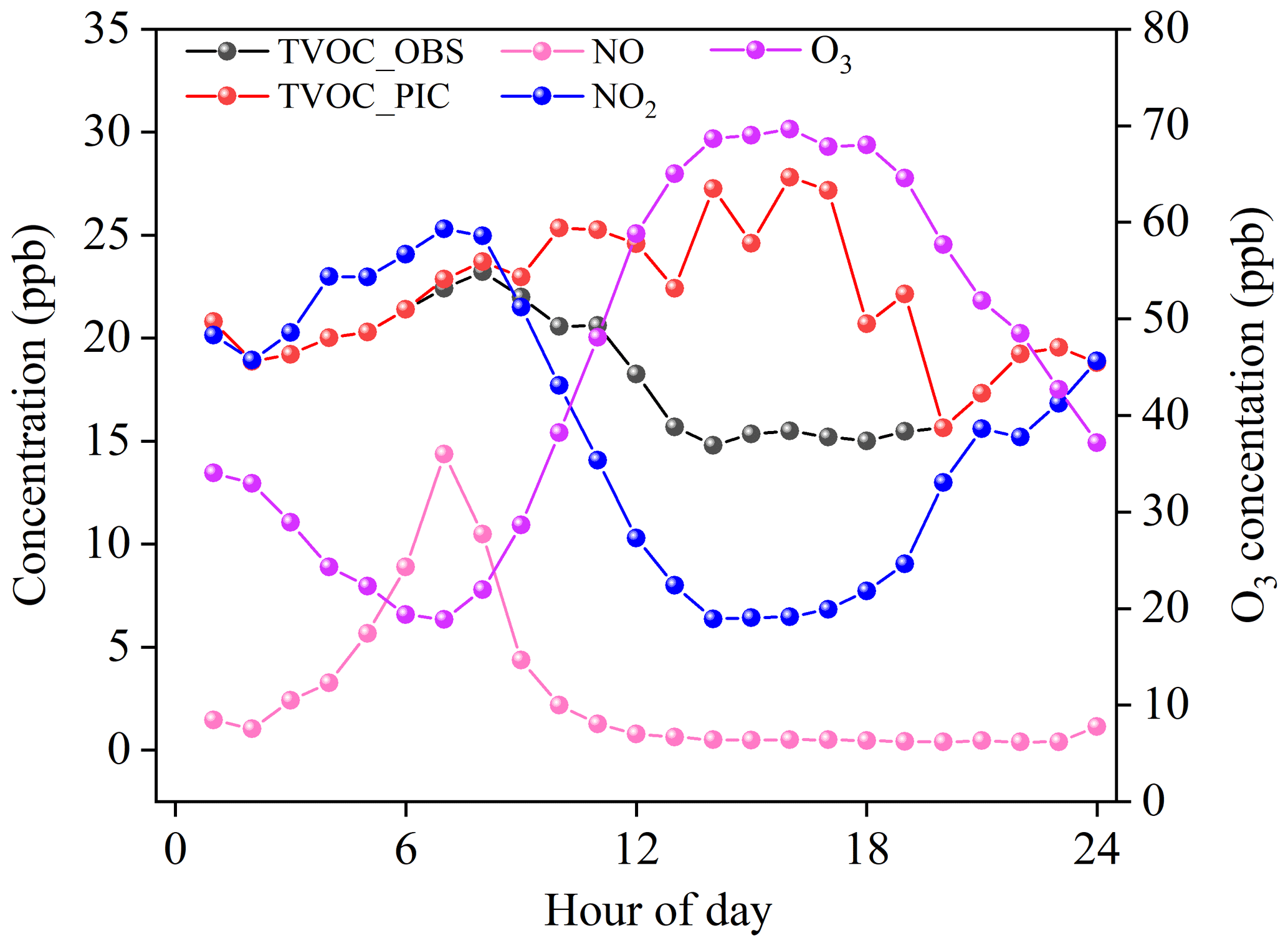
Figure 1 Overview of average diurnal variations in O₃, NO_x, and TVOC. The data represent measured results, except for those of the TVOC_PIC, which are calculated based on OH radical exposure. The data range is 1–28 August 2019.

3.2 Influence of photochemical loss of VOCs on the O₃ formation sensitivity regime

The sensitivity of O₃ formation is analyzed using the isopleth diagram generated from the EKMA model, which is widely used to qualitatively study O₃-NO_x-VOCs sensitivity. As described in Sect. 2.4, the concentrations of NO₂ and VOCs were artificially scaled to ±75 % of the observed values to calculate the response of O₃ concentration to an imaginary change in the concentrations of NO₂ and VOC, with other constrained conditions remaining unchanged. Figure 2 shows the typical EKMA curves during our observations. The black stars and pentagons denote the observed concentrations of NO_x and VOCs in the morning (09:00–10:00 LT) and at noon (14:00–15:00 LT), respectively, while the blue symbols are the corresponding values of PICs. Based on the measured data, O₃ formation was in a VOC-limited regime in the morning and a NO_x-limited regime in the afternoon. The black arrow indicates a linearly decreasing trend of NO_x and VOCs from 09:00 to 15:00 LT in the chemical coordinate system, and ozone production shifted from VOC-limited to NO_x-limited conditions from morning to afternoon, which was consistent with the mean diurnal profiles (Fig. 1). This was similar to the data reported in Wangdu (Tan et al., 2018). As expected, ozone production shifted from a VOC-limited regime (the observed VOCs) to a transition regime based on the PIC-VOCs in the morning. Ozone production clearly moved further to a NO_x-limited regime in the afternoon after the photochemically consumed NO_x and VOCs had been accounted for (Fig. 2). Because the average photochemical aging time was only 1.7±0.9 h, these results indicated that the O₃ formation mechanism might typically be misdiagnosed, which misleads mitigation measures for O₃ prevention if the consumed VOCs under real atmospheric conditions are not considered.

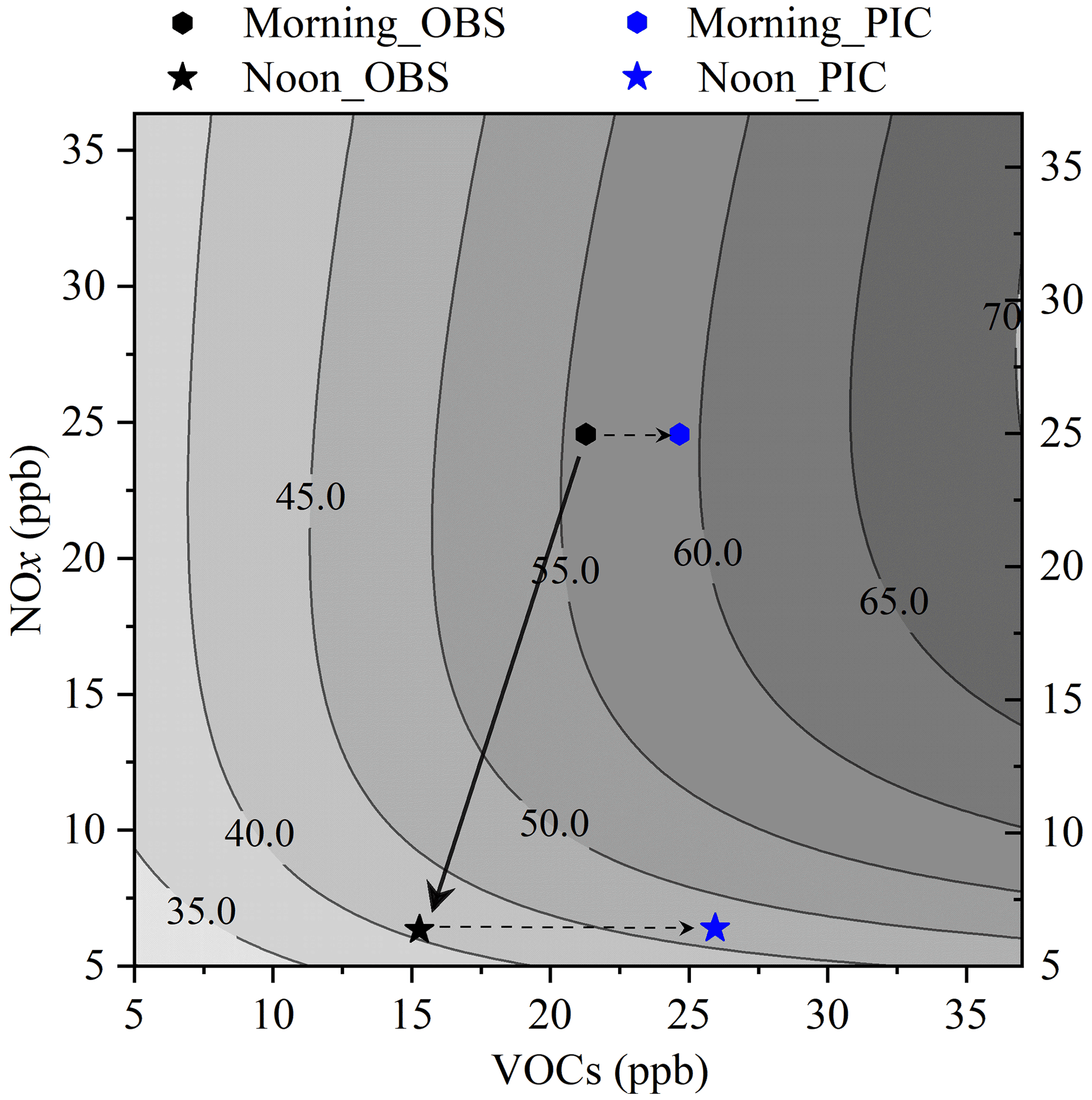
Figure 2 Isopleth diagram of the ozone concentration as a function of the concentration of NO_x and VOCs derived from an empirical kinetic modelling approach. The pentagons and stars indicate the status in the morning (09:00–10:00 LT) and at noon (14:00–15:00 LT), respectively. The black and blue colors represent the observed and corrected statuses, respectively.

3.3 Contribution of VOC species to O₃ production

The time series of simulated OH, HO₂, and RO₂ concentrations were used to calculate the P(O₃) and L(O₃). The diurnally averaged P(O₃) and L(O₃) are shown in Fig. 3. Ozone formation can be divided into processes related to RO₂+NO and HO₂+NO (Sect. 2.3). According to their VOC precursors, peroxyl radical groups were divided into alkane-derived (ALKAP), alkene-derived (ALKEP), aromatic-derived (AROMP), isoprene-derived (ISOP), oxygenated-VOC-derived (OVOCP), and halohydrocarbon-derived (HALOP) RO₂ and HO₂P. The ozone destruction processes included the reaction between O₃ and HO_x (O3D1), the reaction between O¹D and H₂O (O3D2), the reaction between O₃ and alkenes (O3D3), and the reaction between NO₂ and OH (O3D4).

Based on the observed VOCs (or PIC-VOCs), a fast O₃ production rate was observed at 14:00 LT (or 13:00 LT), with a diurnal maximum value of 16.1 (or 25.6) ppb h⁻¹ (Fig. 3a and 3b), while the peak destruction rate was 6.4 (or 8.6) ppb h⁻¹ at 15:00 LT (or 13:00 LT) (Fig. 3c and 3d). The average daytime P(O₃) from 07:00 to 19:00 LT based on the initial concentrations of VOCs was 4.0±3.1 ppb h⁻¹ higher than that based on the measured VOCs concentrations (Fig. 3b). At the same time, the F(O₃) from 07:00 to 19:00 LT based on the initial concentrations of VOCs was also 3.0±2.1 ppb h⁻¹ higher than the measured counterpart (Fig. S12). Thus, the net O₃ production could be accumulatively underestimated by ∼36 ppb d⁻¹ from 07:00 to 19:00 LT if the consumption of VOCs was not considered. This meant that the contribution of the local formation of O₃ could be underestimated using the directly measured VOCs concentrations. It should be pointed out that it is better to compare O₃ production with the true metric for O₃ production. However, it is impossible to directly measure the true metric for O₃ production in the atmosphere at the present time to know how well the method presented here corrects for that underestimation. In addition, the ozone concentrations must be constrained when simulating the ozone formation process (Lu et al., 2013; Tan et al., 2017). Thus, it is impossible to directly compare the ozone production based on PIC-VOCs with that using measured VOCs concentrations. Therefore, we alternatively compared the integrated net ozone production rates rather than ozone production or concentrations between the two scenarios. An upwind O₃ and VOCs measurement combined with a trajectory analysis might provide an approach for checking the accuracy of our results. Alternatively, conducting a transient O₃ production rate analysis after subtracting the transport of O₃ with a regional model and/or satellite observation might be another option. Unfortunately, neither the upwind measurement nor the regional model simulation was available at the time of our study. To further check the accuracy of our results, we chose 4 August as a test case to explore the influence of the transport of ozone on a downwind site based on the trajectory analysis. As shown in Fig. S13, the mean ozone concentration of the downwind site (national monitoring station, NMS) was 27.6±21.9 ppb d⁻¹ higher than that of the observation site (OS), which was slightly less than the difference (∼36 ppb d⁻¹) between PIC-VOCs and observed VOCs and indirectly rationalized our results.

The HO₂ path contributed 64.8 % to the total ozone formation on average, which was slightly higher than the reported value (57.0 %) in Wangdu (Tan et al., 2018), whereas the RO₂ path, in which aromatics (9.4 %), alkenes (8.4 %), isoprene (7.8 %), alkanes (4.7 %), OVOCs (4.3 %), and halohydrocarbons (0.6 %) were the main contributors, contributed to the remaining part. For the PIC-VOCs, the dominant path of O₃ production (51.7 %) was still the HO₂ path, followed by the RO₂ path related to alkenes (14.7 %), aromatics (12.8 %), and isoprene (11.7 %). The relative contribution of the RO₂ path to P(O₃) increased by 13.4 % compared with the measured VOCs, particularly alkene-derived RO₂, which increased by 10.2 %. As shown in Fig. 3c and 3d, the destruction of total oxidants was dominated by the reaction between O₃ and alkenes (O3D3) in the morning. It gradually shifted to the reaction between NO₂ and OH (O3D4) from 11:00 to 16:00 LT and the photolysis of O₃ followed by a reaction with water (O3D2) from 12:00 to 15:00 LT because O₃ concentration increased while NO₂ decreased (Fig. 3c). Figure S14 shows the percentages of the different paths of P(O₃) and L(O₃). The relative contributions of the reactions between O₃ and alkenes (O3D3) and between NO₂ and OH (O3D4) to the O₃ sinks decreased when calculated based on PIC-VOCs compared with those of the measured VOCs, while they obviously increased for the other two paths, i.e., O3D1 and O3D2. The O₃ destruction of the HO_x and O₃ reaction (O3D1) gradually increased with the continuous photochemical reaction. In addition, the maximum O₃ formation rates of the RO₂ derived from OVOCs and halohydrocarbons were 0.75 and 0.18 ppb h⁻¹, respectively. These values could be underestimated due to the incomplete gas reaction mechanism of OVOCs and halohydrocarbons in MCM3.3.1. In general, the measured VOCs as model inputs could fail to truly reflect the oxidation capacity and underestimate the local formation of O₃ and organic aerosols (Zhan et al., 2021).

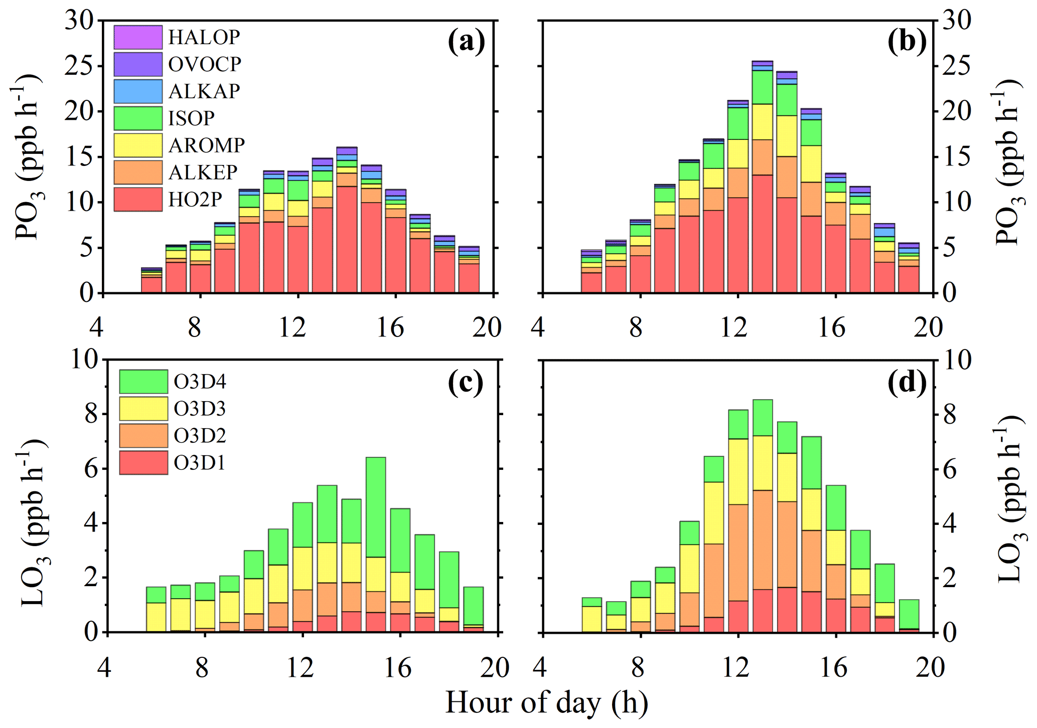
Figure 3 Mean diurnal profile of the instantaneous ozone production and destruction rate calculated from the MCM-OBM model (instantaneous ozone rate derived from observed VOCs in a and c and from PIC-VOCs in panels b and d). The upper panels present the speciation of the ozone formation rate. The lower panels present the speciation of the ozone destruction rate. The data range is 1–28 August 2019.

The budget of OH–HO₂–RO₂ radicals was further analyzed to understand the photochemical O₃ formation process. The comparison of the radical budget derived from the observed and PIC-VOCs is shown in Fig. 4. The radical cycles are divided into radical sources (green boxes), radical sinks (black boxes), radical propagations (red circles), and equilibria between radical and reservoir species (yellow boxes). The numbers or percentages are the average formation rates (ppb h⁻¹) or relative contributions of the corresponding reaction path based on the observed VOCs (outside the brackets) and the PIC-VOCs (inside the brackets) to a certain radical. The relative contributions of different radical paths based on the observed VOCs (outside the brackets) were comparable with those reported in Beijing, Shanghai, and Guangzhou (Tan et al., 2019), while variations were observed for some reaction paths based on the PIC-VOCs. For example, the reaction between ozone and alkenes based on initial VOC concentrations (percentages inside the brackets) contributed more to OH (from 7 % to 21 %) and HO₂ radical production (from 6 % to 12 %), while photolysis of HONO and HCHO contributed less to the production of OH (from 76 % to 60 %) and HO₂ radicals (from 44 % to 40 %), respectively. Other radical sources were consistent between the two scenarios. Interestingly, the average formation rates of OH, HO₂, and RO₂ radicals derived from the PIC-VOCs were obviously higher than those from the observed VOCs. In particular, the oxidation of NO by RO₂ and HO₂ increased by 1.6 and 1.3 ppb h⁻¹, respectively. The enhanced oxidation rate of NO was equal to the increase in the average F(O₃) in the analysis process above. This meant that the radical propagation of OH–RO₂–HO₂ sped up in the case of PIC-VOCs, subsequently accelerating the chemical loop of NO-NO₂-O₃. For the radical sinks and equilibria related to HNO₄, RONO₂, and PAN, the values were basically comparable between the two scenarios. In addition, the O₃ formation from the RO₂ path increased by 4.1 % (from 39.5 % to 43.6 %) in the simulation using the PIC-VOCs compared with the observed VOCs. The above budget analysis explained the observed increases in F(O₃) (∼3 ppb h⁻¹), which were mainly driven by the reaction of missed reactive VOCs, such as alkenes, with O₃.

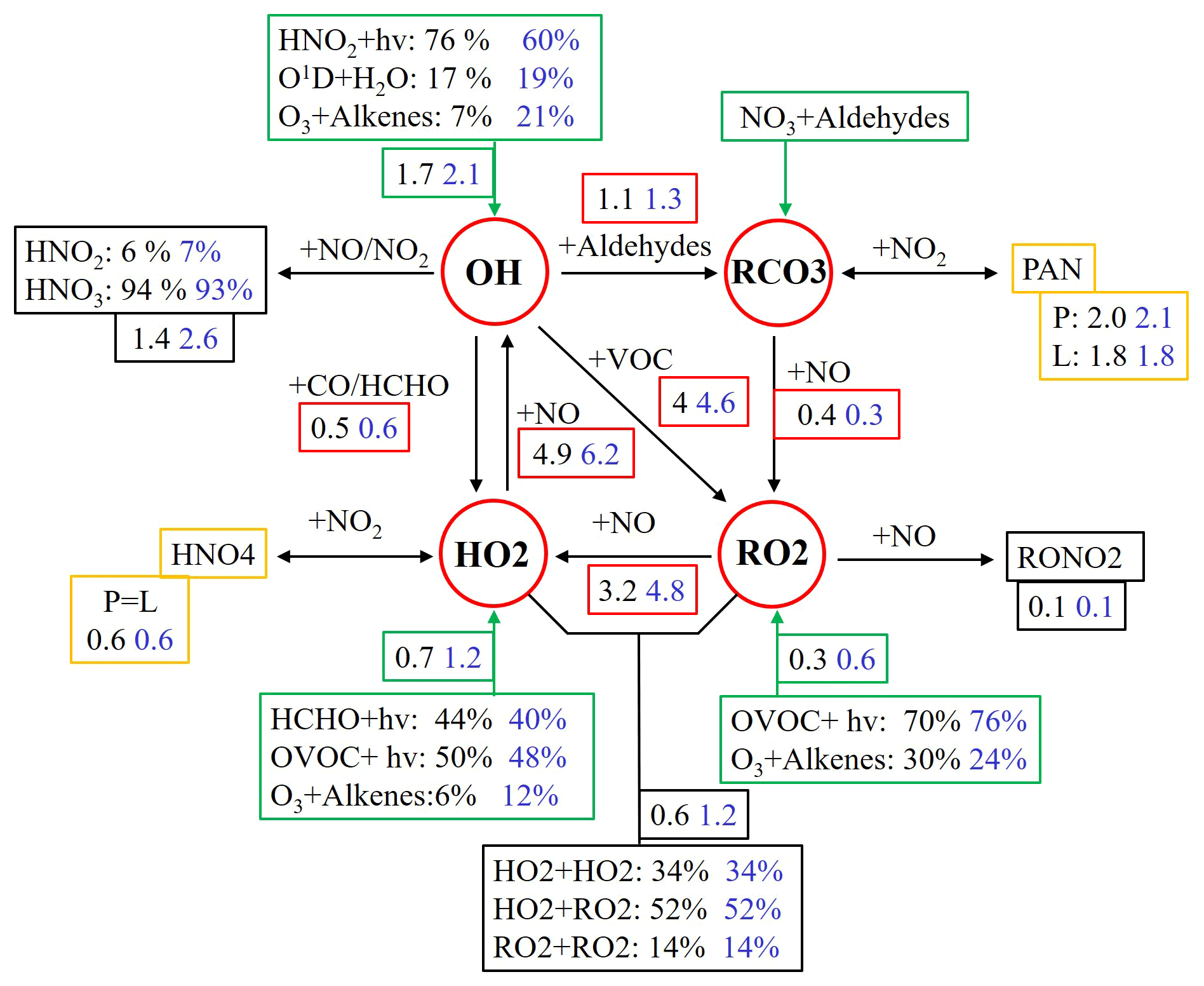
Figure 4 Comparison of the OH–HO₂–RO₂ radical budget derived from the observed and PIC-VOCs under daytime conditions (07:00 to 19:00 LT). The green, black, red, and yellow boxes denote the sources of radicals, radical sinks, radical propagation, and racial equilibrium, respectively. The numbers or percentages outside and inside the brackets are the average formation rates (ppb h⁻¹) or relative contributions to a specific radical of the corresponding reaction path based on observed VOCs and PIC-VOCs, respectively.

3.4 In situ O₃ formation process

In addition to chemical processes, which can be simulated using the OBM-MCM model, transport processes, including horizontal, vertical transportation, and dry deposition processes (Tan et al., 2019), also have an important influence on the O₃ concentration. Thus, the change in instantaneous ozone concentration can reflect the combined effect between photochemical and physical transport processes (Tan et al., 2019). This change can be expressed as follows:

$$\begin{array}{}\text{(6)}& {\displaystyle \frac{{\mathrm{dO}}_x}{\mathrm{d}t}}=F\left({\mathrm{O}}_{\mathrm{3}}\right)+R\left({\mathrm{O}}_{\mathrm{3}}\right),\end{array}$$

where ${\mathrm{dO}}_x/\mathrm{d}t$ is the O₃ concentration change rate based on the measured data (ppb h⁻¹), F(O₃) is the net O₃ formation rate (ppb h⁻¹), and R(O₃) indicates transportation (ppb h⁻¹). A positive value of R(O₃) indicates an inflow of O₃ with air mass and vice versa. O₃ was replaced with O_x (O₃+ NO₂) to correct the titration of O₃ by NO (Pan et al., 2015).

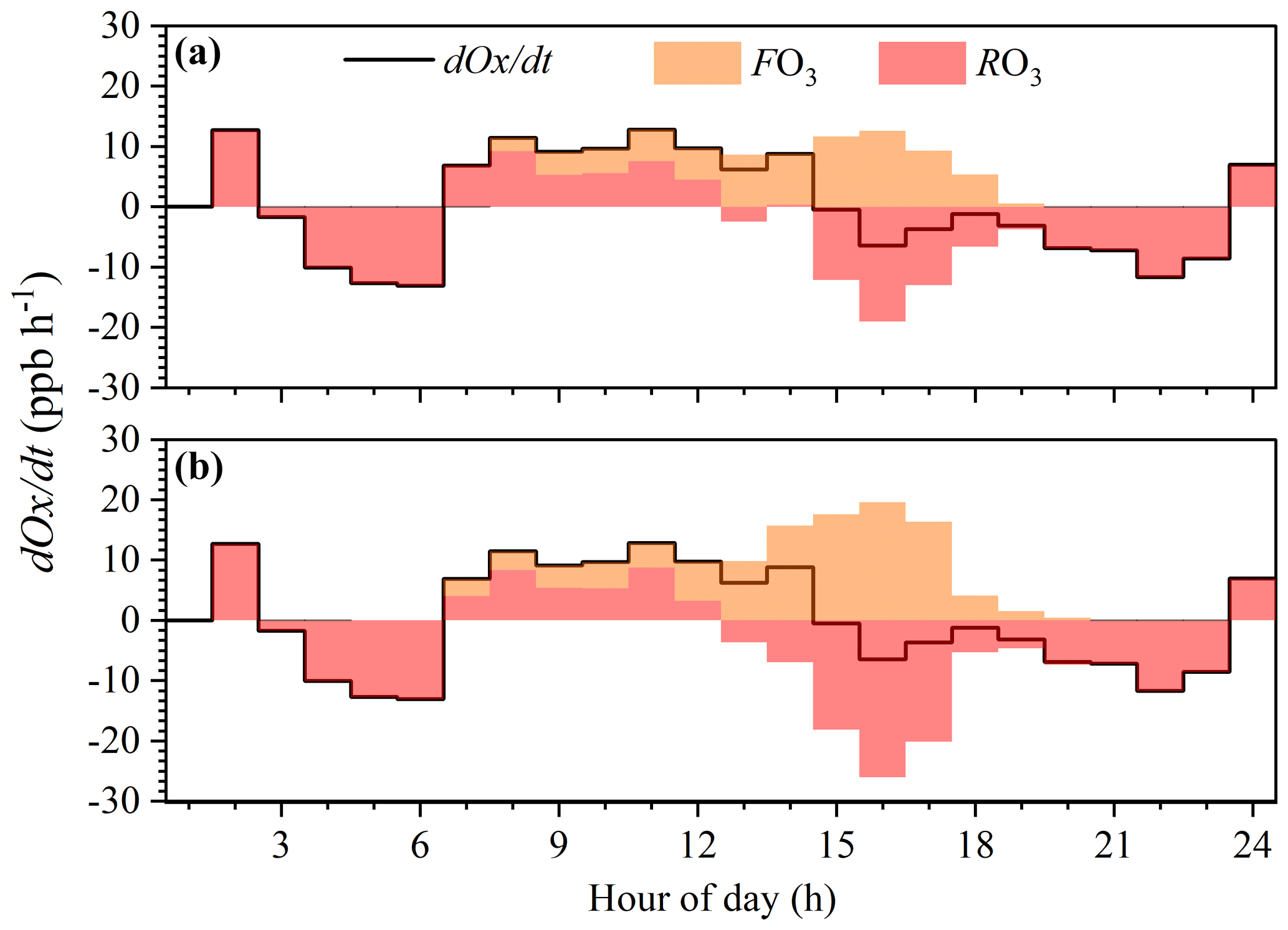
Figure 5 The variation in O_x concentration and formation rate during an O₃ pollution episode (1 August). Panels (a) and (b) present the local ozone formation processes of the measured and PIC-VOCs, respectively.

The O₃ budget analysis was performed during an O₃ pollution episode (1 August). Figure 5 shows the simulated local ozone formation process based on the measured and PIC-VOCs. The hourly variation in O₃ concentrations from 19:00 to 6:00 LT the next day was dominated by regional transportation without O₃ formation, while local photochemical O₃ formation could explain all or part of the O₃ concentration change during the time window from 07:00 to 19:00 LT. The d(O${}_{\mathrm{3}})/$dt shows an increase from 07:00 to 15:00 LT. However, d(O${}_{\mathrm{3}})/$dt sharply changed to negative values at 16:00 LT, which was consistent with diurnal O₃ (the O₃ peaks at 15:00 LT) in Fig. 1.

The average daytime F(O₃) based on the observed and photochemical initial concentrations was 6.4±4.0 and 8.9±6.7 ppb h⁻¹, respectively. Photochemical O₃ formation under both conditions started at 07:00 LT and reached maximum values of 12.6 and 19.6 ppb h⁻¹ at 15:00 LT, respectively. The maximum daily value of P(O₃) was higher than those in the urban areas of Japan, America, and England (Whalley et al., 2018; Ren et al., 2006; Griffith et al., 2016; Kanaya et al., 2009) and lower than those in the suburbs of Guangzhou (Lu et al., 2012) and the urban areas and suburbs of Beijing (Lu et al., 2013). Before 12:00 LT, the O₃ formation rate based on the PIC-VOCs was slightly higher than that based on the measured VOCs, while both rates were within a range of 2.0–6.5 ppb h⁻¹. From 12:00 to 17:00 LT, the O₃ formation rate based on the PIC-VOCs and the observed concentration of VOCs greatly increased due to active photochemistry.

As shown in Fig. 5, the increased O₃ concentration was larger than the local O₃ photochemical production from 07:00 to 12:00 LT (R(O₃) was positive). This was mainly because the nighttime residual layer (RL) is isolated from mixing with the nighttime surface layer under stable conditions (Tan et al., 2021). The RL usually contains an air mass with a higher ozone mixing ratio than in the surface layer. In the morning, surface heating causes mixing upward in the surface layer until the temperature inversion is eroded away and rapid mixing of pollutants throughout the surface and boundary layer occurs. However, R(O₃) was negative in the afternoon, which indicated that the local O₃ formation at the measurement site contributed to not only the changes in the in situ O₃ concentration but also the O₃ source of the downwind regions. This was more clearly shown in Fig. 4b under the PIC-VOC conditions. These results illustrated that local O₃ photochemistry played a crucial role in both the local and regional O₃ concentrations, which can be underestimated if consumed VOCs with high reactivities are ignored.

4 Conclusions

In this study, we presented the local O₃ formation process in August 2019 in Beijing based on the concentrations of observed VOCs and PIC-VOCs. The mean diurnal profile of O₃ was unimodal with a peak at 15:00 LT, while NO_x and observed TVOCs showed an opposite diurnal curve, and the PICs of TVOCs showed a different diurnal curve compared with that of the observed VOCs, with a slight increase from 07:00 to 14:00 LT. The EKMA curve indicated that instantaneous O₃ production was dependent on the real-time concentrations of NO_x and VOCs, i.e., the VOC-limited regime in the morning (09:00–10:00 LT) and the NO_x-limited regime at noon (14:00–15:00 LT). The sensitivity regime of O₃ formation could be misdiagnosed if the consumed VOCs are not considered; for example, the VOC-limited regime (observed) shift to a transition regime (PIC-VOCs) in the morning is ignored. The mean F(O₃) based on PIC-VOCs was 3.0 ppb h⁻¹ higher than that based on the measured VOCs, indicating that the underestimation of local photochemistry in the local O₃ concentration could reach ∼36 ppb d⁻¹ if the consumed VOCs are not accounted for. The mean ozone concentration of downwind site was 27.6 ppb d⁻¹ higher than the observation site, slightly lower than the difference (∼36 ppb d⁻¹) between PIC-VOCs and observed VOCs, which indirectly supported the accuracy of the above results. The radical budget analysis explained the observed increases in F(O₃) (3 ppb h⁻¹), which were mainly driven by the reaction of missed reactive VOCs, such as alkenes, with O₃. In addition, the OH–HO₂ radical cycle was obviously accelerated by highly reactive alkenes after the photochemical loss of VOCs was accounted for. Finally, the results of the in situ O₃ formation process indicated that local O₃ photochemical formation played a key role in both local and regional O₃ concentrations. In conclusion, our results suggested that PIC-VOCs were more suitable than the observed VOC concentrations for diagnosing O₃ formation sensitivity.