the Creative Commons Attribution 4.0 License.
the Creative Commons Attribution 4.0 License.
 | 12 Apr 2022
Assessing the potential for simplification in global climate model cloud microphysics
Sylvaine Ferrachat
David Neubauer
Martin Staab
Ulrike Lohmann
Cloud properties and their evolution influence Earth's radiative balance. The cloud microphysical (CMP) processes that shape these properties are therefore important to represent in global climate models. Historically, parameterizations in these models have grown more detailed and complex. However, a simpler formulation of CMP processes may leave the model results mostly unchanged while enabling an easier interpretation of model results and helping to increase process understanding. This study employs sensitivity analysis of an emulated perturbed parameter ensemble of the global aerosol–climate model ECHAM-HAM to illuminate the impact of selected CMP cloud ice processes on model output. The response to the perturbation of a process serves as a proxy for the effect of a simplification. Autoconversion of ice crystals is found to be the dominant CMP process in influencing key variables such as the ice water path and cloud radiative effects, while riming of cloud droplets on snow has the most influence on the liquid phase. Accretion of ice and snow and self-collection of ice crystals have a negligible influence on model output and are therefore identified as suitable candidates for future simplifications. In turn, the dominating role of autoconversion suggests that this process has the greatest need to be represented correctly. A seasonal and spatially resolved analysis employing a spherical harmonics expansion of the data corroborates the results. This study introduces a new application for the combination of statistical emulation and sensitivity analysis to evaluate the sensitivity of a complex numerical model to a specific parameterized process. It paves the way for simplifications of CMP processes leading to more interpretable climate model results.
- Article
(14435 KB) - Full-text XML
- BibTeX
- EndNote


Aerosols and cloud microphysics (CMPs) control cloud properties and thereby exert a large influence on Earth's climate. For example, the cloud water and ice contents determine the cloud albedo and lifetime, and they also control precipitation formation (Mülmenstädt et al., 2015). In a changing climate, the correct representation of clouds is especially important to estimate Earth's radiation budget (Sun and Shine, 1995; Tan et al., 2016; Matus and L'Ecuyer, 2017; Lohmann and Neubauer, 2018). However, clouds and cloud feedbacks are a major source of uncertainty for projections of climate sensitivity in global climate models (Cess et al., 1990; Soden and Held, 2006; Williams and Tselioudis, 2007; Boucher et al., 2013).
Since cloud microphysical processes such as the riming of cloud droplets on snowflakes occur on scales much smaller than the resolution of global climate models (GCMs), they are parameterized; i.e., only their macroscopic effects at the scale of the model grid are described. Responding to the challenge of incorporating these processes in climate models, the community has added more and more processes into GCMs (Knutti and Sedláček, 2013) with increasing detail in their representation (e.g., Archer-Nicholls et al., 2021; Morrison et al., 2020). As Fisher and Koven (2020) argue for a similar situation in land surface modeling, this may be due on the one hand to scientists' tendency to focus on their own area of expertise. On the other hand, it also reflects the fact that the Earth system is indeed complex and that many processes may matter. However, it is doubtful whether more detail will help us to reduce uncertainty (Knutti and Sedláček, 2013; Carslaw et al., 2018). More complexity also has its downsides: more parameterized processes lead to more parametric uncertainty, which in turn scientists investigate and try to reduce with large scientific effort (e.g., Rougier et al., 2009; Lee et al., 2011; Yan et al., 2015; Williamson et al., 2015; Dagon et al., 2020). In fact, Reddington et al. (2017) argue that “aerosol–climate models are close to becoming an overdetermined system with many interacting sources of uncertainty but a limited range of observations to constrain them”, referring to the complexity in the representation of aerosols and their interaction with clouds. This is related to equifinality, meaning that model versions from different regions of the input parameter space may lead to the same results that compare well with observations. These models may simulate a range of aerosol forcings (Lee et al., 2016), which is not possible to constrain with current observations. Morrison et al. (2020) diagnose the same problem for CMP schemes, whose complexity they say is “`running ahead' of current cloud physics knowledge and the ability to constrain schemes observationally”. Climate models have become so complex that they are impossible to comprehend by any one scientist (Fisher and Koven, 2020). More detail means more heterogeneity between climate models, which increases the difficulty of a meaningful comparison of their projections (Fisher and Koven, 2020). But also within a given model, the attention and detail given to some cloud microphysical processes come at the expense of other less accessible processes. This brings the danger of overinterpreting those processes that are represented in detail while neglecting the impacts of poorly represented ones (Mülmenstädt and Feingold, 2018). Finally, the detail of the aerosol and cloud microphysics increases computational demand and thereby costs (though anticipating the results of Sect. 3.6, the four CMP processes investigated in this study require negligible computing time). It can thereby inhibit other advancements such as the move towards high-resolution simulations (which may themselves also require adaptations of the CMP schemes) or larger ensembles.
In contrast, simple models are easier to interpret and derive understanding from, as long as they represent processes correctly (Koren and Feingold, 2011; Mülmenstädt and Feingold, 2018). Also, assumptions and their consequences are more traceable in simpler or more system-oriented models (Mülmenstädt and Feingold, 2018). For example, conceptual cloud models have been used to investigate the impact of the choice of precipitation particle attributes on the cloud structure and evolution (Wacker, 1995) or to confirm microphysics findings qualitatively (Wood et al., 2009). Simplifications reduce computational demand, and simplified models yield themselves to other applications, e.g., the use in integrated assessment models (Ghan et al., 2013). At the same time, they may produce similarly good results as more complex models. For example, Ghan et al. (2012) developed a simple yet physical model for the aerosol indirect effect, whose estimates are comparable to those of complex global aerosol models. Similarly, Liu et al. (2012) compared two aerosol modules with seven and three lognormal modes and find that the simulated aerosol concentrations are remarkably similar.
The addition of detail and refinement of a model description is a natural response to the challenge of capturing something as complex as the climate system in a computer model. This is legitimate and beneficial. For example, it may lead to a physically more correct representation and reduce the number of tuning parameters (e.g., Storelvmo et al., 2008). And for some applications modelers may need as much detail as possible in one specific module. Hence, scientists tend to call for more detail in process representations (e.g., Gettelman et al., 2013, for warm-rain microphysics; Sotiropoulou et al., 2021, for secondary ice production by break-up from collisions between ice crystals) instead of less. This may in part be because humans are biased towards searching for additive pathways as problem solutions while overlooking subtractive transformations (Adams, 2021). However, due to the reasons mentioned above, a simplified model equifinal to a more complex model may be more useful for gaining understanding of climate models (equifinal meaning that the two model versions lead to similar results). One can therefore question the need for an ever increasing amount of detail, especially in the face of overdetermination (Reddington et al., 2017). In this paper, we propose a new methodology to assess where process parameterizations can be stripped of detail to aid the development of a simplified model as well as to increase understanding of the model.
The role of CMPs within GCMs has been investigated previously: the influence of CMPs has been shown to dominate over that of aerosol schemes in affecting clouds and precipitation in the Weather Research and Forecasting model (White et al., 2017), as well as to dampen the influence of aerosol microphysics on cloud condensation nuclei and ice-nucleating particles in a regional model (Glassmeier et al., 2017). For the HadGEM-UKCA global aerosol–climate model, Regayre et al. (2018) have shown that both aerosol and physical atmosphere parameters contribute to uncertainty in aerosol effective radiative forcing. Diving into the importance of single processes for the overall CMPs, Bacer et al. (2021) extracted process rates from the chemistry–climate model EMAC, which is based on the same CMPs as this study's ECHAM-HAM. They found that ice crystal sources in large-scale clouds are controlled by freezing and detrainment from convective clouds, while sinks are dominated by autoconversion and accretion. This approach is somewhat similar to a pathway analysis (e.g., Schutgens and Stier, 2014; Dietlicher et al., 2019) in that it deepens understanding of immediate effects but is not able to relate the effect of a process on variables further down the process chain.
A promising method for investigating the effect of model input on output is the use of perturbed parameter ensembles (PPEs) (Murphy et al., 2004; Collins et al., 2011). In a PPE multiple input parameters are perturbed at the same time. In this way, PPEs expand upon sensitivity studies that vary one parameter (e.g., Lohmann and Ferrachat, 2010; He and Posselt, 2015) or multiple parameters at a time (e.g., Ghan et al., 2013), allowing the investigation of the interaction effects of perturbations within the whole possible parameter space. For example, Sengupta et al. (2021) used a PPE to determine the impact of parameters related to secondary aerosol formation on organic aerosol in a global aerosol microphysics model. In a next step, parameter ranges can be constrained when comparing the PPE to observations (Posselt, 2016; van Lier-Walqui et al., 2014, 2019, note that these studies all used synthetic observations as constraints). Morales et al. (2021) built a PPE of CMP process parameters and environmental conditions, generated using a Markov chain Monte Carlo algorithm, in idealized simulations to then constrain the parameters with synthetic observations.
Another benefit is that a PPE does not require any additional changes to model code, in contrast to a pathway analysis that requires additional diagnostics and tracers. The downside is that PPEs require many simulations to sample the whole parameter space, which is prohibitive given the cost of global climate model simulations. A remedy is the combination of a PPE with a surrogate model such as an emulator. The emulator is first fitted to the PPE model output and then sampled instead of the GCM, which is expensive to run. This technique has been used, for example, to study the effect of model parameters such as the entrainment rate coefficient on climate sensitivity in a GCM (Rougier et al., 2009) or how model parameters affect forecast model drift (Mulholland et al., 2017).
Global sensitivity analysis is a method to quantify the effect of inputs on model output more formally. It allows us to divide the total variation in output into the direct contributions from variations in independent inputs as well as from their interactions. For example, Tan and Storelvmo (2016) used variance-based sensitivity analysis on a generalized model of their PPE to determine that the Wegener–Bergeron–Findeisen timescale is the most influential parameter in determining the cloud-phase partitioning in mixed-phase clouds. Bernus et al. (2021) have employed sensitivity analysis of their PPE directly to improve the understanding of their lake model prior to its implementation into a climate model.
When dealing with large models that are expensive to run, a surrogate model that is cheap to run allows for a tight sampling of the whole parameter space which permits for sensitivity analysis on the resulting surface. As such, the combination of a PPE with a surrogate model upon which sensitivity analysis is performed has found wide use in cloud simulation studies (Wellmann et al., 2018; Glassmeier et al., 2019; Wellmann et al., 2020; Hawker et al., 2021a). For example, Lee et al. (2011) emulated a global aerosol model and found that the cloud condensation nuclei concentration in polluted environments is dominated by sulfur emissions but that in remote regions interactions between different parameters are substantial. In particular, a range of recent studies has employed the methodology to investigate how uncertainty in input parameters (which are often not well constrained within parameterizations) translates to an uncertainty of climate model output: quantifying the effect of aerosol parameters on cloud properties or radiative forcing (Lee et al., 2011, 2012; Carslaw et al., 2013; Lee et al., 2013; Regayre et al., 2014; Johnson et al., 2015; Regayre et al., 2015; Yan et al., 2015; Regayre et al., 2018), but also in various other areas of environmental modeling (e.g., a land model in Dagon et al., 2020). In a further step, the effect of an observational constraint on the model output can be investigated with the emulator as a surrogate model (Tett et al., 2013; Williamson et al., 2013; Lee et al., 2016; McNeall et al., 2016; Johnson et al., 2018), yielding important conclusions about which observations are needed to constrain climate models and on which parameters we need to focus research efforts. The approach also lends itself to an investigation of tuning parameters since these also form a parameter space that needs to be explored and constrained (Williamson et al., 2015; Hourdin et al., 2020; Couvreux et al., 2021).
Here we propose a new application of the combined PPE and sensitivity analysis approach to learn about the needed accuracy in process parameterizations within GCMs. Instead of varying parameters within parameterizations, we perturb the processes themselves as a whole. By perturbing we mean that we vary the effectiveness of a given process, going from using 50 % to 200 % of a process's effect in the model. For example, if a process affects the ice crystal number concentration, the change induced on it is multiplied by a perturbation factor between 0.5 and 2 in each time step. This means that in the extreme cases it would produce half or twice the effect on the ice crystal number concentration that it has in the default model (see Sect. 2.2 for further detail). From the resulting response surface we infer the sensitivity of model output to the CMP processes. The thus generated understanding points to processes whose representation needs to be accurate since they have a large influence and suggests simplifying those processes that have little influence on model output. Accepting the notion of equifinality, we aim to identify the parts of our current model that do not contribute to variation in output. Thus, we develop a “global sensitivity analysis that can weed out unimportant parameters” as called for by Qian et al. (2016).
To avoid misunderstanding, we are using a surrogate model to learn about sensitivities within the ECHAM-HAM GCM. We are not aiming to replace CMP parameterizations with machine learned substitutes (as e.g., Seifert and Rasp, 2020) or substitute model components (e.g., Beusch et al., 2020) because interpretable, physics-based models should be preferred (Rudin, 2019). Instead, in line with Couvreux et al. (2021) we are using emulation and sensitivity analysis as a tool to generate understanding that allows us to build a more interpretable model version in a second step. Please note that the potential for simplification is evaluated in the current climate. Thus, any derived simplifications would need to be evaluated against a reference model for their suitability in a changed climate state prior to employing it in, e.g., climate change projections.
In Sect. 2 the CMP processes that we investigate, their treatment in the ECHAM-HAM GCM, the generation of the PPE and emulator, and the sensitivity analysis are described. In Sect. 3 the results from a “one-at-a-time” sensitivity study that explores the axes of the parameter space (Sect. 3.1), the emulated PPE (Sect. 3.2), and the sensitivity study on the fully sampled parameter space (Sect. 3.3) including a scale dependency (Sect. 3.4) and seasonal analysis (Sect. 3.5) are presented and discussed. Conclusions and an outlook are given in Sect. 4.
2.1 Cloud microphysics in ECHAM-HAM
This study employs the global aerosol–climate model ECHAM6.3-HAM2.3 (Tegen et al., 2019; Neubauer et al., 2019), with a T63 horizontal spectral resolution and 47 vertical levels. The cloud microphysics consist of a two-moment prognostic scheme for ice crystals and cloud droplets, with additional one-moment prognostic representation of snow and rain (Lohmann and Roeckner, 1996; Lohmann et al., 1999; Lohmann, 2002; Lohmann et al., 2007; Lohmann and Hoose, 2009; Lohmann and Neubauer, 2018). The stratiform cirrus scheme includes homogeneous nucleation of supercooled liquid droplets (Kärcher and Lohmann, 2002a, b; Lohmann, 2003). The stratiform liquid cloud scheme encompasses condensation, aerosol activation, autoconversion of cloud droplets to rain, accretion of cloud droplets by rain, evaporation of cloud and rainwater, and wet scavenging of aerosol particles (for further details and references see Neubauer et al., 2019). In stratiform mixed-phase clouds, various CMP processes are included: heterogeneous nucleation via immersion and contact freezing, depositional growth of cloud ice, growth of ice crystals at the expense of cloud droplets via the Wegener–Bergeron–Findeisen process (Wegener, 1911; Bergeron, 1935; Findeisen, 1938), and sublimation and melting of ice crystals and snow below clouds. In this study, we are investigating the effect of four different CMP processes involving the ice phase (see Fig. 1). Self-collection of ice is the process of ice crystals sticking together to form a single ice crystal. Autoconversion also has two ice crystals sticking together, albeit forming a snowflake. In accretion, a snowflake collects an ice crystal, resulting in a larger snowflake. The fourth process is the only one involving the liquid phase: cloud droplets are riming on a snowflake, again enhancing its size. The implementation of these processes in terms of changes to the ice crystal and cloud droplet mass is detailed in Lohmann and Roeckner (1996), while the implementation of changes to the ice crystal and cloud droplet number concentration is simply in proportion to the mass changes (except for where the mass concentration is unaffected; Lohmann et al., 1999; Lohmann, 2002). The distinction between accretion and autoconversion is necessary due to the separation between ice crystals and snowflakes in their representation as categories of ice in the model. Snowflakes precipitate, while ice crystals are smaller and sediment but do not survive outside clouds. The four processes were chosen for their comparability, as they all represent particle interactions, to represent a range of assumed impacts, as well as for their implementation, which is clearly distinguishable in the code and allowed for easy implementation of the perturbations (see Sect. 2.2). In this study, we do not include any ice multiplication processes. Convective clouds are treated separately from stratiform clouds, except for the interaction through detrained condensate from convective clouds, which is added to stratiform clouds if they exist at the respective model level.
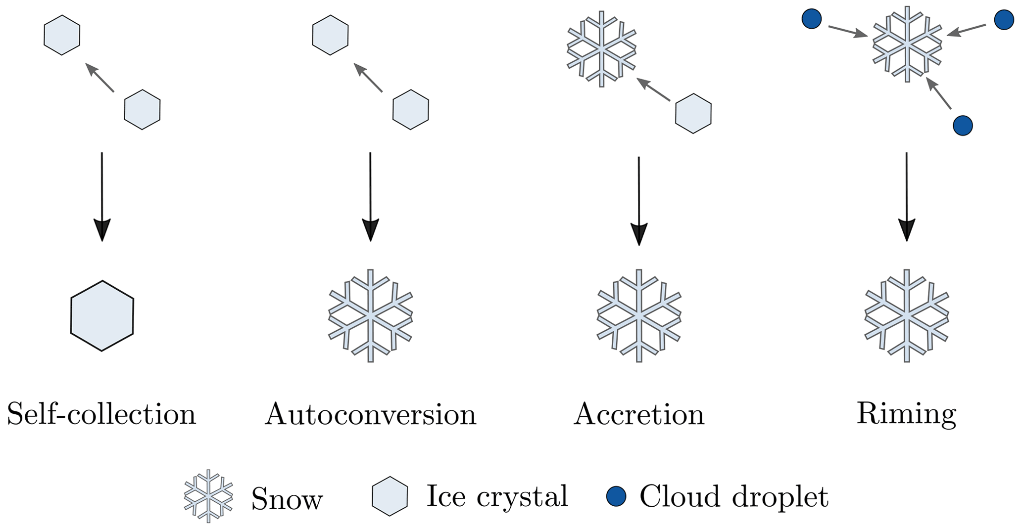
Figure 1The four cloud microphysical processes investigated in this study, depicted as they are represented in ECHAM-HAM.
Apart from the perturbations described in the next section, substantial changes that were applied with respect to the published model version ECHAM6.3-HAM2.3 (Neubauer et al., 2019) are the following.
-
Detrained condensate from the convective cloud scheme produced an unrealistically large amount of ice crystals at mixed-phase temperatures, which were then removed with a correction term. The detrained cloud particles are now assumed to be all liquid at mixed-phase temperatures (0 ∘C < T < −35 ∘C; Dietlicher et al., 2019; Muench and Lohmann, 2020).
-
In line with Muench and Lohmann (2020, Sect. 3.3.1.2), we now include the immediate, updraft-dependent self-collection of detrained ice crystals.
-
Previously, a fixed minimal cloud droplet number concentration (CDNC) was applied, which led to unrealistically high CDNCs in high-latitude and/or high-altitude clouds with low liquid water content (LWC) and hence small droplets. We replace this with a dynamically calculated minimal CDNC, which is calculated from the in-cloud water content and a set maximum volumetric cloud droplet radius (set at 15 µm in the simulations conducted for this study). The resulting minimum CDNC needs to lie between 106 and 4 × 10⁷ m−3. Admittedly, we are replacing the tuning parameter of fixed minimum CDNC with one for a maximum cloud droplet radius. The latter is preferred as it is more physical.
-
The model version of Neubauer et al. (2019) contains a mistake in the calculation of the hygroscopicity parameter in the aerosol activation parameterization, leading to an underestimation of the individual aerosol-mode solubility. The calculation was updated in Friebel et al. (2019) and subsequently used in Lohmann et al. (2020); this correction is also applied here.
-
In part motivated by the large correction terms highlighted in the process rate study of Bacer et al. (2021) we reduce these if they are unnecessary and/or unphysical. For example, conditions of maximum ice crystal number concentration (ICNC) were enforced after a few CMP processes took place in Bacer et al. (2021). We could reduce the value of that correction term by applying it after each relevant process. Most importantly, the diagnosis of multiple correction terms acting on the same variable led to an artificial increase in corrections. For example, correction terms would enhance ICNC concentrations at model points that later were identified to be outside a cloud (due to the way the code is structured, the diagnosis of cloud cover happens after, e.g., activation and/or nucleation takes place). In turn, ICNCs outside a cloud were then corrected to be zero, so an unnecessary correction was in fact counted twice. We reduce this artifact by correcting the correction terms themselves. Staying with the example above, the first correction term is now itself set to zero outside a cloud.
-
The sublimation of sedimenting ice crystals appears to be too weak in ECHAM-HAM. This became apparent as in-cloud ICNCs were increasing through sedimentation from above, which indicates that sublimation of ice crystals falling into the cloud-free part of a grid box is too weak. While the underlying problem of a weak sublimation needs to be addressed with future efforts, we introduced a correction of the sedimentation routine: the gain of ice crystal concentrations in the level k into which the ice crystals sediment, ΔICNCsed,k, is restricted to the loss of in-cloud ice crystal number concentration in the lowest model level above level j that lost ice crystals by sedimentation. Also, in-cloud ICNC and the snow formation rate are now set to 0 outside clouds inside the ice crystal sedimentation routine wherein they were previously set to the grid-mean values. This contains the implicit assumption that ice crystals do not survive sedimentation outside a cloud in ECHAM-HAM.
With the described changes, the model requires retuning. The tuning procedure follows the one described in Neubauer et al. (2019), with the final tuning parameters given in Table A1 in Appendix A. Model simulations were conducted with the same tuning for all simulations.
2.2 Perturbations as a proxy for complexity
In order to see the effect of whole processes on model output, we can turn processes off in sensitivity studies. In the present study, we achieve this by setting the change that the process induces on prognostic variables to zero. For example, at every model time step t autoconversion impacts the ICNC:
We can turn off the effect of autoconversion by multiplying ΔICNCautc, the change in ICNC due to autoconversion in one time step, by zero when it is added to the affected variables.
More generally, instead of setting the changes induced by a process to zero, we can perturb the process using a newly defined parameter η.
This perturbation of whole processes was introduced by van Lier-Walqui et al. (2014) to estimate the uncertainty including errors in the physical assumptions of process formulations. In our case, the parameters aid understanding the sensitivity of the model to each process: from the response of model output to variations in ηi, we can extract information on how accurately a process i needs to be represented in the model (see Fig. 2 for a visualization). For example, if the model output variable (e.g., ice water path, IWP) as a function of ηi has a slope close to zero at ηi=1 (green and purple line in Fig. 2), this suggests that the process i needs to be represented only approximately and that some detail could probably be removed from its parameterization without much of an effect on the model performance. Note that the perturbations are constant in space and time for each PPE member, serving as a proxy for understanding the effect of possible simplifications, which would likely be variable in time and space. In this study, four cloud microphysical processes, namely self-collection, autoconversion, accretion, and riming (see Fig. 1), are perturbed, i.e., . Combining perturbations of multiple processes allows us to study and take into account possible interaction effects, such as the compensation by one process which is perturbed by another one.
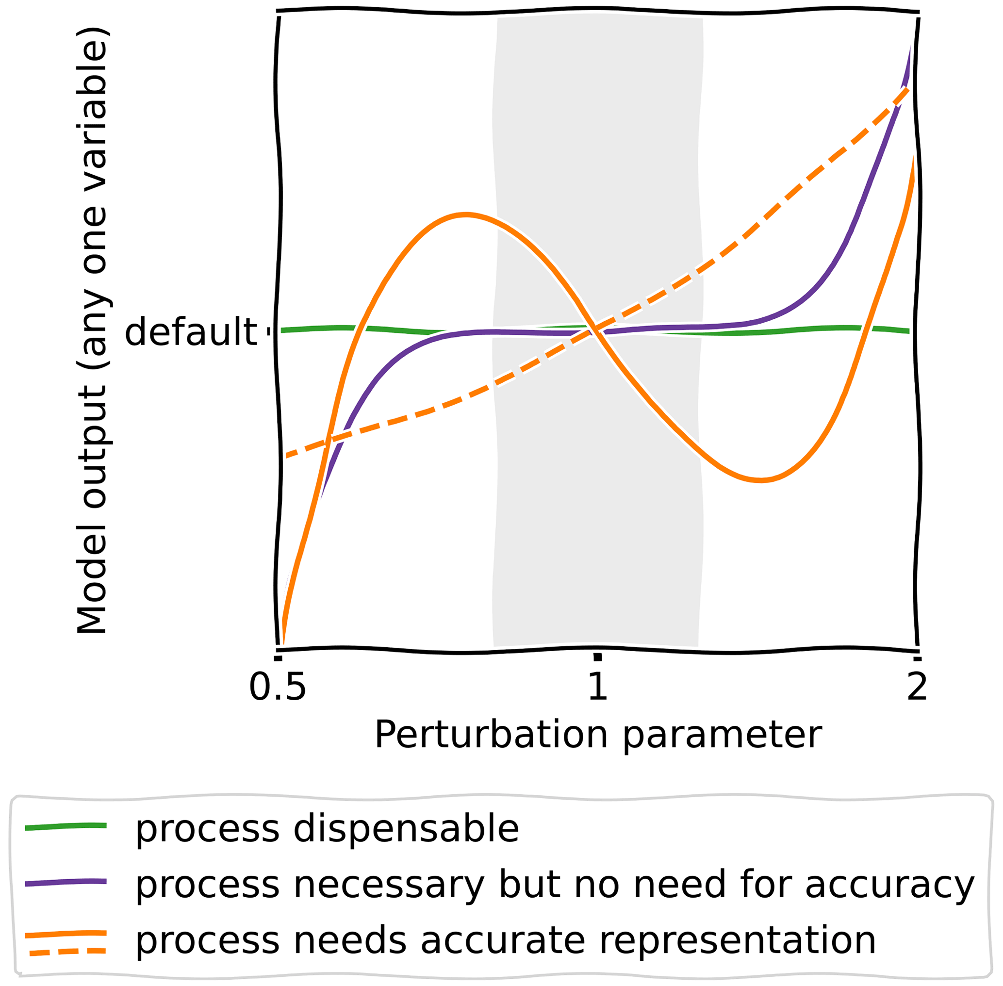
Figure 2Sketch of the envisioned interpretation. The shading indicates the area that is of most interest to judge the effect of process simplifications on the model output. If the slope in this area is small, this suggests that the process can be simplified (green and purple lines). A large slope indicates that the process needs to be represented accurately (orange lines). If no perturbations of the process in the 0.5 to 2 perturbation parameter range and the suppression of the process (perturbation parameter of 0, not shown) have a significant influence on the model output, the process may be removed entirely (green line).
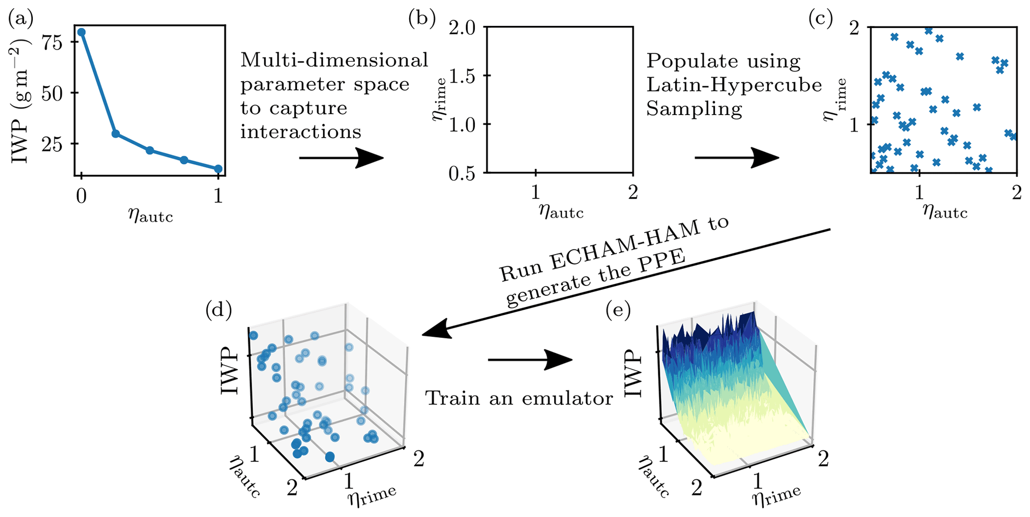
Figure 3Sketch of the employed methodology: we move from (a) one-dimensional sensitivity studies wherein one process is perturbed by varying the parameter η (Sect. 3.1) to (b) a multidimensional parameter space. (c) The input parameter space is filled with Latin hypercube sampling and supplied as input to ECHAM-HAM. The simulations form the perturbed parameter ensemble (PPE). The (d) PPE output is (e) fitted using a Gaussian process emulator for each variable of interest to generate a smooth response surface, upon which sensitivity analysis can be applied. Note that this is an illustrative sketch of the method for a PPE with two input dimensions, whereas our PPE has four dimensions, and that the data used to generate it are only illustrative as well. The shading in (d) illustrates depth only.
2.3 Generating and emulating the perturbed parameter ensemble (PPE)
In a first scoping study, we perturb each process one by one by multiplying its effect with . Multiplicative perturbations between zero and 1 correspond to a reduction in the effectiveness of the process. However, to take into account interactions, all ηi values need to be varied at the same time, thereby creating a multidimensional input parameter space in a second step. In addition, the range of ηi is expanded to values up to ηi=2 to imitate an overestimation of a given process due to an inaccurate description. As we are most interested in the space around ηi=1, and to sample the over- and underestimation equally, we vary ηi from 0.5 to 2 in the multidimensional input parameter space. If the process uncertainty were known, it would influence the extent of the perturbation range, which could be different for each process. The perturbations and the procedure described in the following are visualized in Fig. 3. To probe the multidimensional input parameter space effectively, the sets of input parameter combinations (η1, η2, η3, η4) to be simulated with the model were generated with Latin hypercube sampling (LHS, using the Python library PyDOE, tisimst, 2021), which maximizes the spacing between inputs and provides good coverage of the parameter space, even when only a few input parameters are important (Morris and Mitchell, 1995). The LHS was applied to the logarithmically scaled input range to account for the multiplicative behavior of the ηi. Each of the LHS-generated input combinations was then used as input for a 1-year ECHAM-HAM model simulation, creating a perturbed parameter ensemble (PPE) with 48 members. This is in line with the suggestion of Loeppky et al. (2009) to use 10 times as many training runs as the number of input parameters for such a computer experiment. To estimate the interannual variability, the control simulation with all processes at full effectiveness () spanned 10 years. This estimate is used to judge whether perturbations observed in the PPE are significantly larger than the interannual variability and therefore contain a signal that originates from the perturbation in ηi. As the interannual variability exhibited no strong variations throughout the probed phase space in the one-at-a-time sensitivity studies, the 1-year simulations for the PPE members in combination with the control simulation estimate of the variability were deemed sufficient for the analysis. All the simulations were performed with climatological sea surface temperatures and sea ice extents, as well as aerosol emissions representative for the year 2003. These simulations were not nudged to meteorological data but ran freely so that the full effect of perturbing the processes could be observed. Each simulation included 3 months of spin-up that was not included in the analysis.
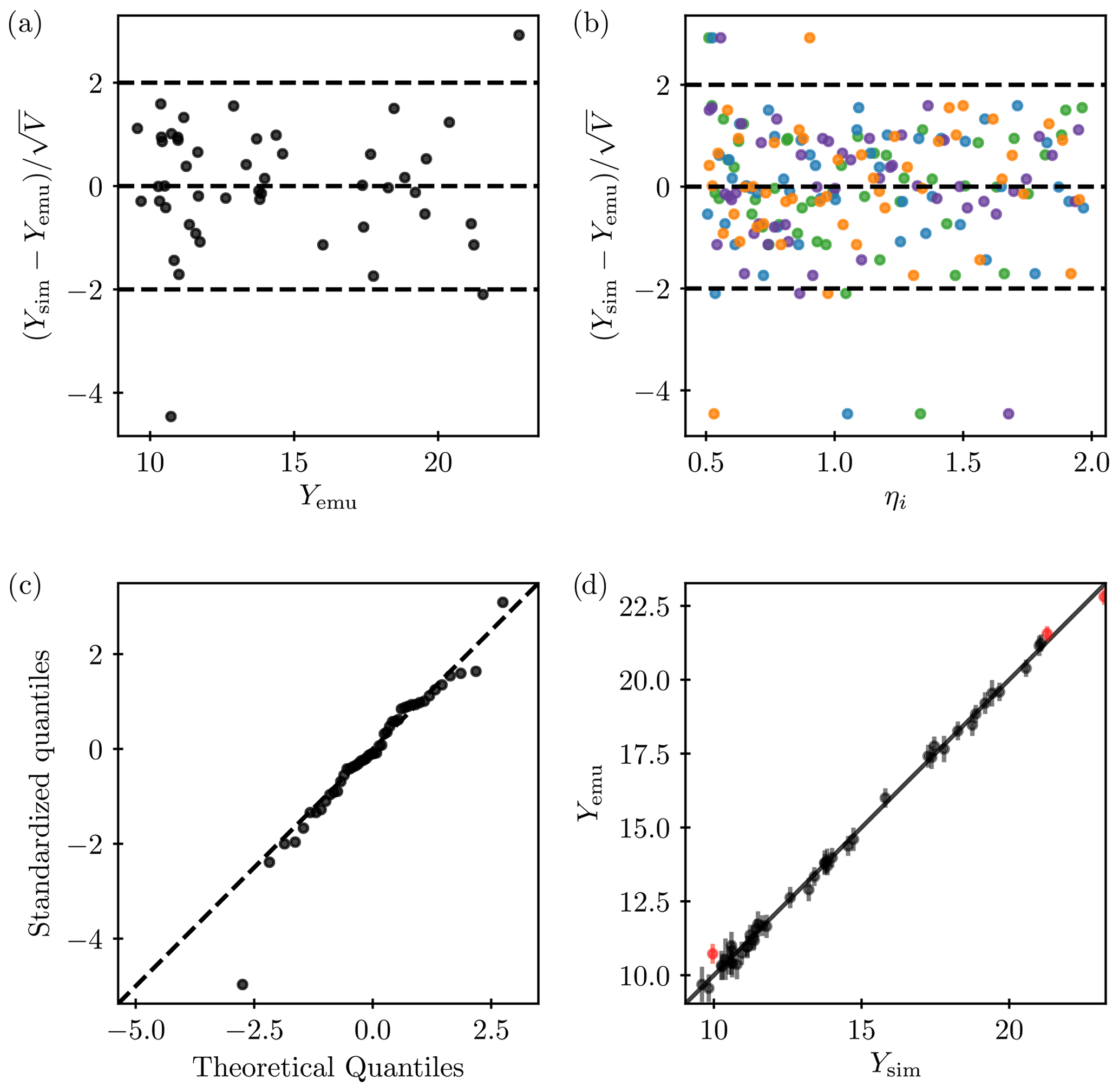
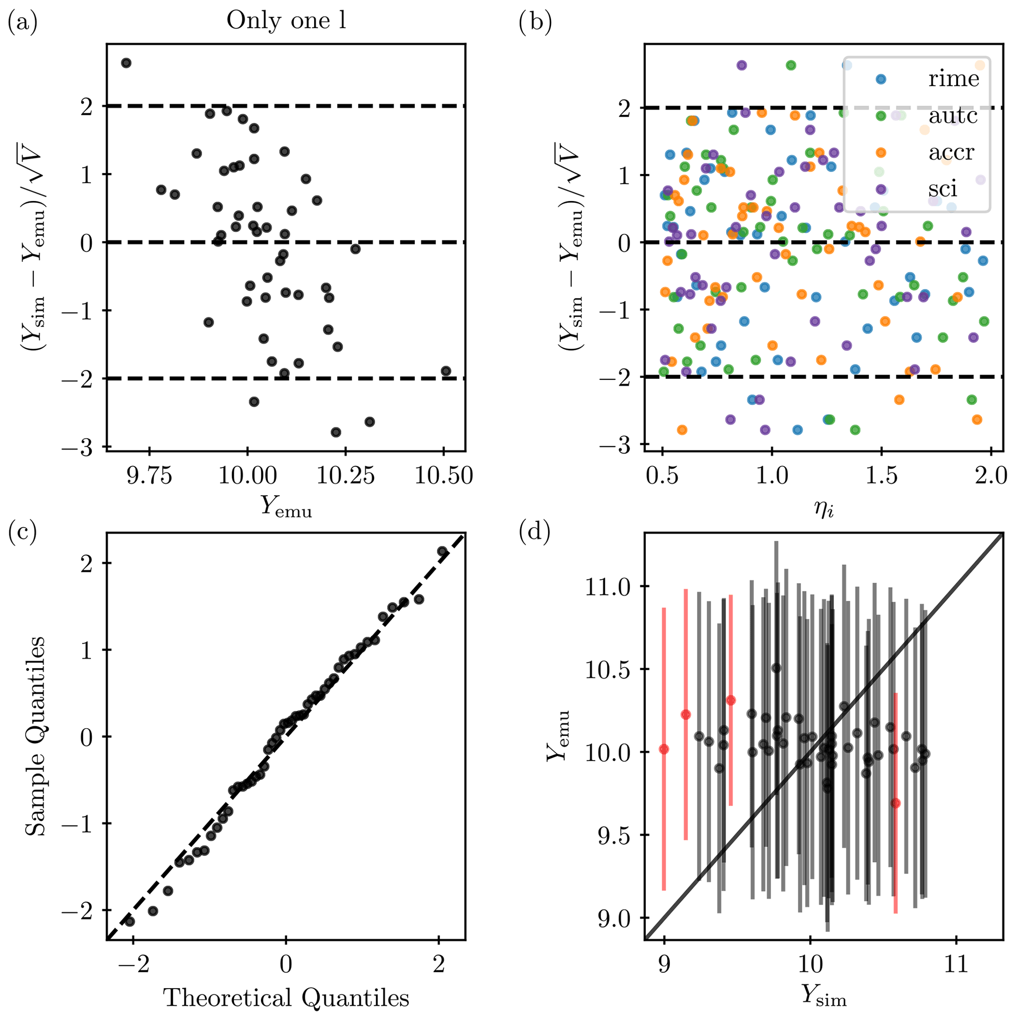
Figure 4Leave-one-out validation of the emulator for global annual mean IWP. Each point corresponds to the training of the emulator on all points except one and then testing on exactly that point. Individual standardized errors are plotted against (a) emulator output and (b) input parameters (colors according to Fig. 5: autoconversion – blue, accretion – purple, riming – green, self-collection – orange). The dashed lines are drawn at an individual standardized error of zero and 2, which is the threshold discussed in Bastos and O'Hagan (2009). (c) Q–Q plot of the individual standardized errors against a Student's t distribution. (d) Emulator against model output, with the error bars indicating the 95 % confidence interval on the emulator predictions. Predictions for which the model result lies outside that interval are marked red.
Using the PPE output as input for the creation of a surrogate model, we can construct a smooth response surface over the whole parameter space (see Fig. 3e). As a surrogate model, we choose a Gaussian process emulator (O'Hagan, 2006; Rasmussen and Williams, 2006), which has found wide use in atmospheric and climate science (Lee et al., 2011; Carslaw et al., 2013; Johnson et al., 2015). We prefer the Gaussian process emulator over, e.g., a neural network because of its demonstrated suitability and need for fewer input data (see Watson-Parris et al., 2021, for a more in-depth discussion). Using a recent Python package for emulating Earth system models (Watson-Parris and Williams, 2021; Watson-Parris et al., 2021), the implementation is straightforward. From the PPE, we can construct a surrogate model for every output variable that we are interested in by training a separate emulator for each output variable (ice crystal and cloud droplet number concentration, ice and liquid water path, shortwave and longwave cloud radiative effect, cloud cover, surface precipitation, ice, liquid, and mixed-phase cloud cover). For the kernel (or covariance function, Watson-Parris et al., 2021), an additive combination of the linear, polynomial, bias, and exponential kernels was used as this performed best in preliminary tests (not shown, Duvenaud, 2014). Other model specifics were set as default in Watson-Parris and Williams (2021). As the emulation operates best on standardized data with zero mean and unity variance, the mean was removed from the input data, which was then scaled by dividing it by the standard deviation, prior to emulation. With the cheap surrogate model a variance-based sensitivity analysis (see Sect. 2.5) becomes feasible (Oakley and O'Hagan, 2004), picking 3000 samples from the emulator as input. This approach is similar to Johnson et al. (2015), except that they perturbed CMP parameters, while we vary the effectiveness of whole CMP processes. It allows us to identify the importance of the different ηi for the variables in question and thereby the processes which require a detailed representation.
2.4 Validation
To make sure that the chosen emulators are a fair representation of the model output, we validate them according to Bastos and O'Hagan (2009) except for using leave-one-out validation, as visualized in Fig. 4 for the IWP. In Fig. 4a and b, the individual standardized errors, (with Ysim and Yemu as the output of the ECHAM-HAM simulations and the emulated output, respectively, and Vemu the emulator variance), are plotted against the emulated output and input parameters. We observe only a few errors larger than 2, which would signal a conflict.
We employ a Q–Q plot to determine whether the normality assumption of a Gaussian process is met in the emulator (Bastos and O'Hagan, 2009). The plot compares the quantiles of the standardized errors against those of a Student's t distribution. Figure 4 c indicates that the normality assumption holds and that the predictive variability is well estimated by the emulator (Bastos and O'Hagan, 2009). In a direct comparison of emulated and simulated ECHAM-HAM model output (Fig. 4d), the points should lie close to the line of equality, with the 95 % confidence bounds on the emulator predictions crossing it. This should be the case for 95 % of the validation points. In our emulations, the number of points with confidence bounds that do not cross the line of equality is sometimes larger (up to 27 %), depending on the variable. We attribute this to the disruptive changes that the CMP process perturbations induce compared to, e.g., the aerosol and CMP parameter changes applied by Johnson et al. (2015) (which did not include ice crystal autoconversion and perturbed parameters only within uncertainty bounds instead of whole processes), as well as to the fact that the simulations were not nudged. The difficulty in emulating the response surface for some of the variables was also apparent in computational limitations: some of the leave-one-out validation emulations were not possible to compute because of numerical instabilities in the computations when constructing the emulator. As these were only a few cases (up to two for global means and four for seasonal means in 48 validation emulations), the validation for those variables as a whole is still deemed valid.
The good qualitative agreement with the line of equality and the lack of systematic errors are sufficient for a validation of the emulator, especially considering that we are not aiming for exact quantitative estimates as results of the presented analysis. Rather, we are looking for a conceptual understanding of the need for an accurate description of CMP processes, for which this emulator validation is sufficient.
For the variables which passed the leave-one-out validation, the final emulator used for the sensitivity analysis was trained on all PPE members (note that in a few cases only 47 PPE members were used due to numerical instabilities in the computations when constructing the emulator). Note that the setup of the emulator includes design choices such as the kernel combination to use. Therefore, the present emulator is only one of multiple possible emulators that could be used to represent the model data. However, as it is shown to validate well, other setups are expected to lead to the same conclusions as this one in the analysis.
2.5 Sensitivity analysis
In our framework, the question of how detailed the representation of a given process i needs to be translates to the question of how sensitive the model output is to a variation of the perturbation parameter ηi. For an answer, we employ variance-based sensitivity analysis, following Saltelli (2008). In contrast to derivative-based local methods (Errico, 1997), global variance-based sensitivity analysis allows for an investigation of sensitivities within the whole input parameter space. Its main metrics are the first- and total-order sensitivity indices (Si and STi, respectively). The first-order sensitivity index of ηi measures the contribution of variance in ηi to the variance in an output variable Y. It is constructed as
E is the average over Y with all η except ηi (η∼i) being allowed to vary while ηi is kept fixed at . Then is the variance over that average for varying . Si is always between 0 and 1, and high values signal an important variable. For additive models all first-order terms add up to 1, i.e., . In non-additive models (e.g., a climate model) interaction terms also have to be taken into account. However, in models with many input parameters the computation of all interaction sensitivities can be cumbersome. The total effect sensitivity index STi offers a remedy in that it summarizes all direct and interactive effects a parameter's variance has on the total variance in output (Homma and Saltelli, 1996; Saltelli, 2008). It is defined as
Here all but ηi (η∼i) are kept fixed at and only ηi is allowed to vary for the average . Then the variance of that average over varying is computed and divided by the variance in output Y. Saltelli et al. (1999) argue that the first and total sensitivity index suffice for a meaningful global sensitivity analysis. To compute these indices via the Sobol method, we make use of the Python library SALib (Herman and Usher, 2017).
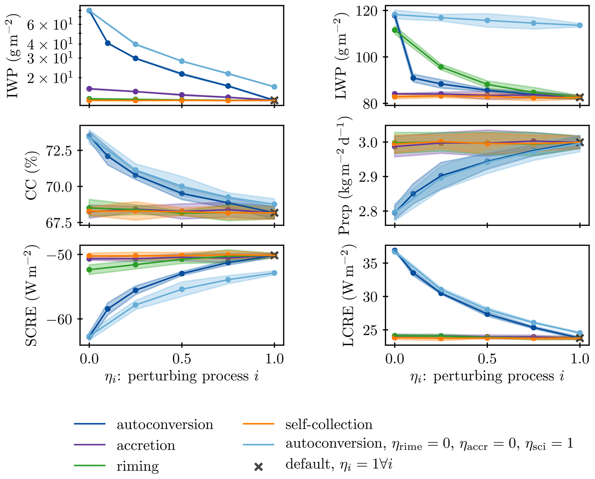
Figure 5Model response to perturbations of four CMP processes: autoconversion, accretion, riming, and self-collection (as illustrated in Fig. 1) in terms of global annual mean IWP, liquid water path (LWP), cloud cover (CC), precipitation (Prcp), and shortwave and longwave cloud radiative effect (SCRE, LCRE). An additional experiment was conducted to highlight interactive effects between the perturbation of autoconversion and the suppression of riming and accretion (light blue). The points and line indicate the mean, and the shading indicates 2 times the standard deviation of annual mean values of a 5-year simulation. Classical sensitivity studies would only show ηi=0 and ηi=1. Note that we added an extra simulation at ηautc=0.1 to better illustrate the threshold behavior discussed in the text and that for the IWP the shading is hidden behind the lines.
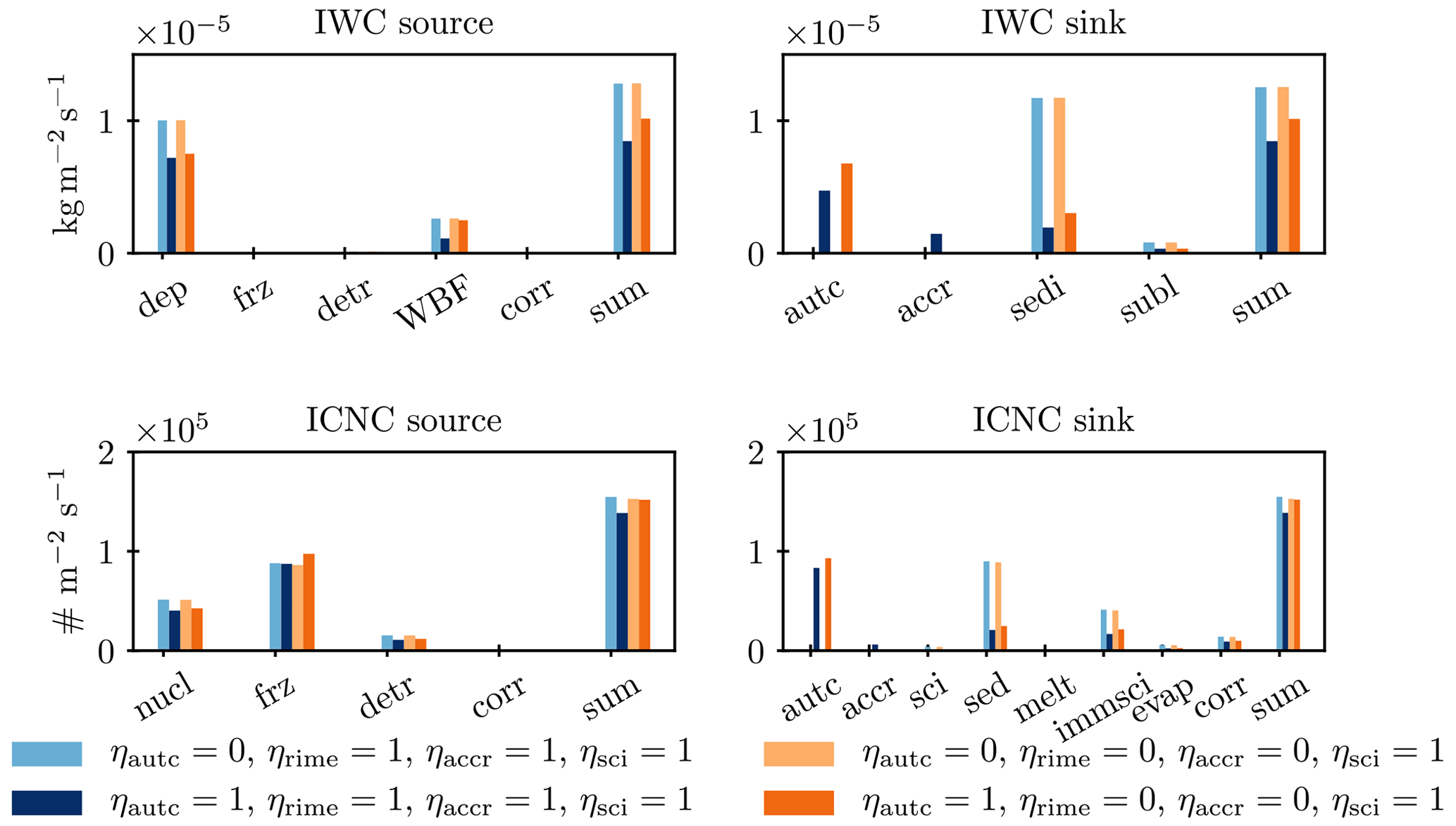
Figure 6Global annual mean vertically integrated process rates for four experiments that illustrate the suppression of snow formation through turning off autoconversion (mean of a 5-year simulation). The rates are diagnosed similarly to Bacer et al. (2021), but correction terms were themselves subtracted from process rates where appropriate, i.e., where the correction belongs to the logical entity of the process rate (see Sect. 2.1). The process rates are deposition (dep), heterogeneous and homogeneous freezing (frz), detrainment (detr), deposition in the Wegener–Bergeron–Findeisen process (WBF), correction terms (corr), autoconversion (autc), accretion (accr), sedimentation (sedi), sublimation (subl), ice nucleation in the cirrus scheme (nucl), melting (melt), immediate self-collection of ice crystals when the ICNC is larger than a maximal threshold (immsci), and evaporation (evap).
3.1 One-at-a-time sensitivity studies
In a first scoping experiment, we perturbed each process separately, which one can imagine as tracing the edges of the cube shown in Fig. 3. The results are presented in Fig. 5. Of the four perturbed processes, turning off autoconversion has the largest effect on model output: the global annual mean ice water path (IWP) is more than doubled, and the increase in cloud cover and decrease in precipitation dwarf the changes induced by turning off the other three processes. In fact, the perturbations induced by perturbing accretion and self-collection are mostly insignificant compared to the interannual variability. As autoconversion is a removal process for ice crystals, it is reasonable that its suppression leads to an increase in ice in the atmosphere (note that the IWP in ECHAM-HAM only counts ice crystals and not snow). Similarly, riming is a removal process for liquid droplets, so the liquid water path (LWP) increases with its suppression. However, surprisingly the suppression of autoconversion induces a similarly large increase in LWP as that of riming, even though autoconversion includes no direct interaction with liquid droplets. The shape of the model response to the gradual perturbation of the processes holds additional information: while the generated model response is mostly gradual, for low ηautc the response is more abrupt. This behavior, which we call a threshold response, is most striking for the global annual mean LWP, for which the signal for ηautc≥0.25 is not significantly different to that of accretion and self-collection. When autoconversion is completely suppressed, the LWP increases dramatically and the signal becomes stronger than that for riming, which had increased consistently and gradually. This behavior can be explained by autoconversion acting as a catalytic process for accretion and riming, creating a threshold behavior when it is turned off. As can be seen from Fig. 1 it is the only process that generates snowflakes. Accretion and riming need the snowflakes to be able to act upon them. Therefore, when autoconversion is turned off, accretion and riming are consequently suppressed as well. In this way, the suppression of autoconversion can strongly influence even the liquid phase. The simulations in which we perturb autoconversion while having riming and accretion turned off confirm this hypothesis (light blue line in Fig. 5): throughout most of the phase space, turning off accretion and riming reinforces the signal from phasing out autoconversion. However, when autoconversion is turned off, turning off accretion or riming does not change the model output any further. That is because they are both suppressed when autoconversion is turned off and does not generate any snow for them to act upon.
Figure 6 further elucidates the reaction of the model to a suppression of autoconversion: the snow formation rate decreases dramatically, and with increased ice concentrations in the atmosphere, the other removal processes of sedimentation and melting subsequently increase. Again the suppression of riming and accretion only influences the model output when autoconversion is active. When autoconversion is turned off, accretion and riming have no influence.
From this one-at-a-time example, one can already see the benefit of the perturbation approach: in classical sensitivity studies, wherein processes are only turned on and off, only the large signal induced by autoconversion would have been visible. However, here it was the peculiar shape of the model response to the whole perturbations that hinted at the threshold effect of autoconversion. The implications for possible simplifications are different: seeing only the large difference between a simulation with and without autoconversion, one would think that this is an immensely important process. Recognizing it as a threshold process and seeing the gradual response to small deviations from 1.0 in ηautc (similar to the purple curve in Fig. 2), it appears that there is potential for a less accurate description of autoconversion in the model. It has also become clear that interaction effects need to be taken into account as well to explain the model behavior. This is what the PPE expands upon in the next section.
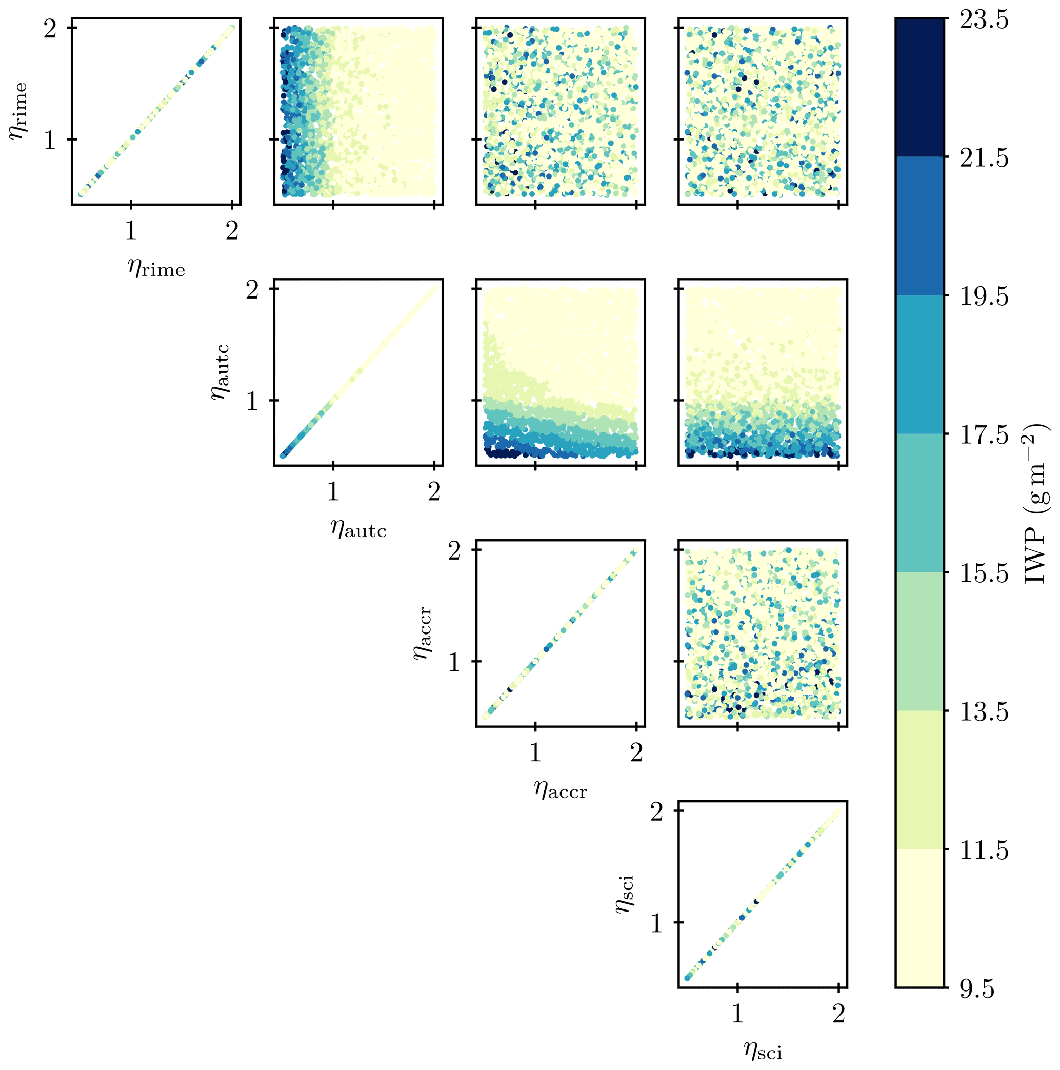
Figure 7Two-dimensional projections of the IWP values sampled from the four-dimensional parameter space of the emulated PPE. Each perturbed process is a dimension, and the color bar denotes the global annual mean ice water path for each input parameter combination.
3.2 PPE of global mean variables
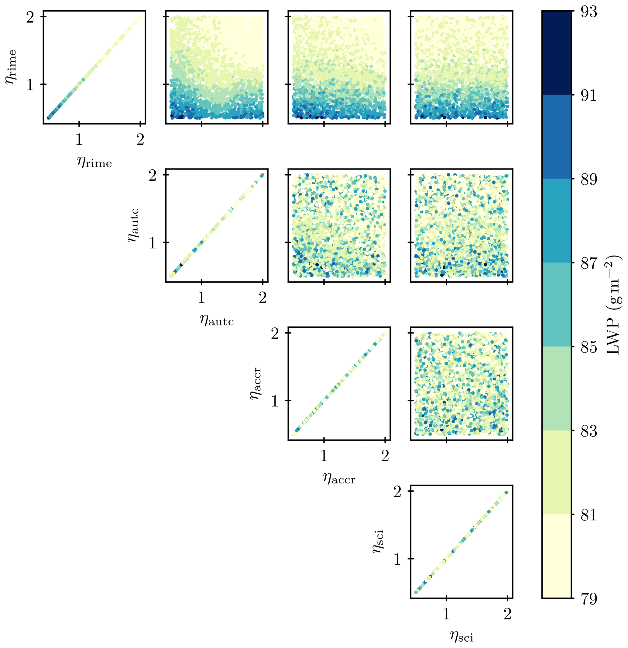
Conducting a 1-year simulation with ECHAM-HAM for each of the 48 input parameter combinations generates the PPE which is then emulated (see Fig. 3). Figure 7 illustrates the resulting response surface with points sampled from that emulation of the annual global mean IWP. To generate the multidimensional response surface 48 1-year simulations were needed compared to the 21 simulations that were needed to investigate the response along only a few of the parameter space edges in Sect. 3.1. This illustrates the value of the chosen approach: the emulated PPE provides more information while needing only roughly twice as many simulations. The surface shows an ordered ascent with decreasing ηautc, while the other dimensions exert no control over the value of the IWP. Only for accretion is a slight influence visible from the tilted contours in the phase space shared with autoconversion. Increased accretion depletes the IWP since it converts ice crystals to snowflakes. Figure 8 shows that the LWP is dominated by ηrime, with an additional influence of autoconversion. The LWP decreases with increasing ηrime and increasing ηautc. This is because riming depletes the atmosphere of cloud droplets and a decrease in autoconversion suppresses riming. The panels in Figs. 7 and 8 exhibiting no order in their parameter space distribution indicate that the processes in question exert no influence on the respective output variable. Similar to the LWP, the CDNC is dominated by riming, and for other cloud variables the dominant influence of autoconversion is confirmed as well (see Fig. B1 in Appendix B).
The ranges in the global annual mean model variables that we observe are mostly larger than what Lohmann and Ferrachat (2010) find for varying uncertain tuning parameters, indicating that whole processes exhibit a larger influence on the model response than those single parameters. Only for LWP do Lohmann and Ferrachat (2010) find a larger range of about 50 gm−2 when they multiply the autoconversion rate with a factor between 1 and 10. As this warm-rain process is not included in the present analysis, it is reasonable that the observed variation for LWP is smaller.
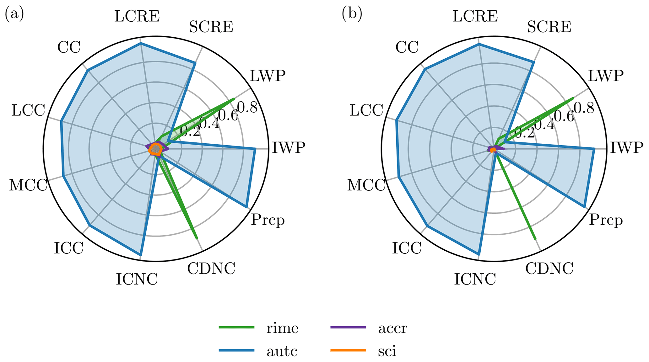
Figure 9First-order (a) and total effect (b) sensitivity indices for the emulated response surface of global annual mean cloud cover (CC), liquid cloud cover (LCC, T > 0 ∘C), mixed-phase cloud cover (MCC, 0 ∘C < T < −35 ∘C), ice cloud cover (ICC, T < −35 ∘C), longwave cloud radiative effect (LCRE), shortwave cloud radiative effect (SCRE), liquid water path (LWP), ice water path (IWP), and total precipitation. As described in Sect. 2.5, the indices are always between 0 and 1, and high values signal an important variable. Since the climate model is non-additive, the terms do not add up to 1 as interactions have to be taken into account.
3.3 Sensitivity analysis
A global variance-based sensitivity analysis allows us to quantify the qualitative sensitivities obtained from the graphical representations of the emulated surfaces in the previous section. The results for the first-order (Si) and total effect (ST) sensitivity indices are presented in Fig. 9. Indeed, the qualitative results are confirmed: the global annual mean LWP and CDNC are dominated by riming, while all other variables are dominated by autoconversion in both first-order and total effect.
The observed sensitivities are different from what Bacer et al. (2021) find in their investigation of EMAC ICNC process rates. They find that autoconversion contributes about twice as much as accretion to the ICNCs, while self-collection has a negligible role. In our analysis, the influence of autoconversion dwarfs that of accretion in terms of sensitivity indices as well as for the process rates (see Fig. 6). The sensitivity indices are not directly comparable to Bacer et al. (2021). However, for the default simulation the process rates are diagnosed as in Bacer et al. (2021) and thus comparable. We attribute the observed differences to the slightly different model version used in Bacer et al. (2021), which goes along with a different tuning.
The almost binary results for the sensitivity indices are surprising, as in other studies the sensitivity indices were more evenly distributed (Lee et al., 2011; Wellmann et al., 2018, 2020). However, these studies usually employed a wider suite of input parameters, whereas here only processes from the limited system of ice particle interactions are included. We expect that with additional cloud microphysical processes included, the sensitivities would be more evenly distributed as well. The binary signal is due to the strong dominance of autoconversion throughout the parameter space and not due to the threshold behavior upon suppression of autoconversion as analyzed in Sect. 3.1. This was excluded from the sensitivity analysis as only the input parameter space with ηautc≥0.5 was taken into consideration.
The dominance of autoconversion is hypothesized to originate from the nonlinearity in its parameterization. In contrast to the other processes, the conversion rate of autoconversion has a squared dependency on the cloud ice content (see Lohmann and Roeckner, 1996), increasing feedback effects between the two.
Additional reasons for the large role of autoconversion may lie in its role as a tuning parameter in ECHAM-HAM. For tuning, uncertain parameters of the model are used (Neubauer et al., 2019). Historically, the scaling factor for the stratiform snow formation rate by autoconversion, γs, has been used as it represents a counterpart to the scaling factor for the stratiform rain formation rate by autoconversion. To reach the tuning goals as detailed in Neubauer et al. (2019), it is brought to unrealistically high values (see Table A1). This enhances the changes induced by perturbing autoconversion in this study using ηautc. Additionally, structural problems in the model may enhance the role of autoconversion artificially. For example, by accounting for heterogeneous nucleation in the cirrus scheme, which increased ice crystal sizes, Gasparini et al. (2018) were able to reduce γs by an order of magnitude compared to the reference ECHAM-HAM version (Blaž Gasparini, personal communication, 2021). This in turn would be expected to reduce the importance of autoconversion in the present analysis. Moreover, the design choices of the CMP scheme, e.g., the order in which processes are called, may also influence the results. However, learning about the properties of CMP processes in the ECHAM-HAM model is important, no matter whether they are physically based or artificially introduced through model design.
A caveat to these results is of course that only CMP processes were investigated here. Parameters or processes from other parts of the climate model, e.g., the dynamics, might exhibit an even larger influence on the investigated model output if they were allowed to be varied. For example, Wellmann et al. (2020), using idealized COSMO simulations, found that environmental conditions are more influential for the diabatic heating rates than microphysical processes. However, for the research question at hand, namely how accurate the representation of these four processes within the CMPs needs to be, the comparison of the processes between each other is sufficient. Indeed, the negligible sensitivity of model output to variations in accretion and self-collection of ice suggests that their representation may be simplified (Lee et al., 2012). Due to the small deviations in the considered variables in response to variations around ηi=1 for riming and autoconversion (purple line in Fig. 2), there is potential for simplifications of their formulations. In the grand scheme of CMP parameterization development, however, autoconversion as the most dominant process of the four is a key process to scrutinize given the possibly troubling origin of this dominance in its role as a tuning factor.
3.4 Scale dependency analysis
The analysis of global annual mean values yields clear conclusions, but climate models need to simulate not only global mean values correctly but also their spatial and temporal evolution. Since the emulation and subsequent analysis of grid-point-level data is tedious and error-prone due to the small signal and large noise, we compress the information in the data to a space of lower dimensionality. Choosing to reduce the dimensionality but still represent the whole global data rather than picking certain regions allows for a more objectified and unbiased analysis. This is similar to Holden et al. (2015), who also reduce their high-dimensionality output, albeit with singular value decomposition, and Ryan et al. (2018), who use principal component analysis. However, as the model data are complete and on a sphere, a spherical harmonics expansion is our method of choice.
Mathematically, the model data can be represented as a linear combination of the orthogonal spherical harmonics basis functions as follows:
The data represented by f are then a function of the longitude θ and latitude ϕ, with a spherical harmonics function of degree l and order m (l and m are integers, with ). The complex coefficients can be computed as
The coefficients make up the angular power spectrum Sff:
where the sum over the angular power spectrum is the variance of the data. In principle, an expansion up to order 95 would represent the model data at their resolution of 96 latitudinal and 192 longitudinal points perfectly, as they are equidistant in spherical coordinates. In practice, we truncated the expansion at the degree l where it represents 95 % of the total data variance . Thereby we represent the data with as few as possible but as many as necessary basis functions. Note that in principle, a principal component analysis could yield the same representation with fewer basis functions. However, these functions would depend on the investigated dataset, while the use of spherical harmonics allows for intercomparability.
Figure 10 illustrates that a spherical harmonics expansion of the data can serve as an accurate representation, while all the information can be stored in the coefficients up to l=20 instead of on the global grid (see Fig. 10c). Thus, confident that the expansion represents the data accurately, we can conduct a spatially resolved sensitivity analysis in the spherical harmonics space. For each variable and degree l a separate emulator was trained on the angular amplitude spectrum , from which samples were drawn as input to the sensitivity analysis. The validation procedure was the same as described in Sect. 2.4. Spherical harmonics members of degree l were excluded from the sensitivity analysis when the emulator was found to be defaulting to an equal prediction over the phase space (see Appendix D). This was the case mostly for degrees l for which the coefficients could already be seen to have less amplitude in the angular amplitude spectrum. A total of 5 out of 11 variables had to be excluded because too many members were defaulting or because their variations were too small to be sensibly emulated.
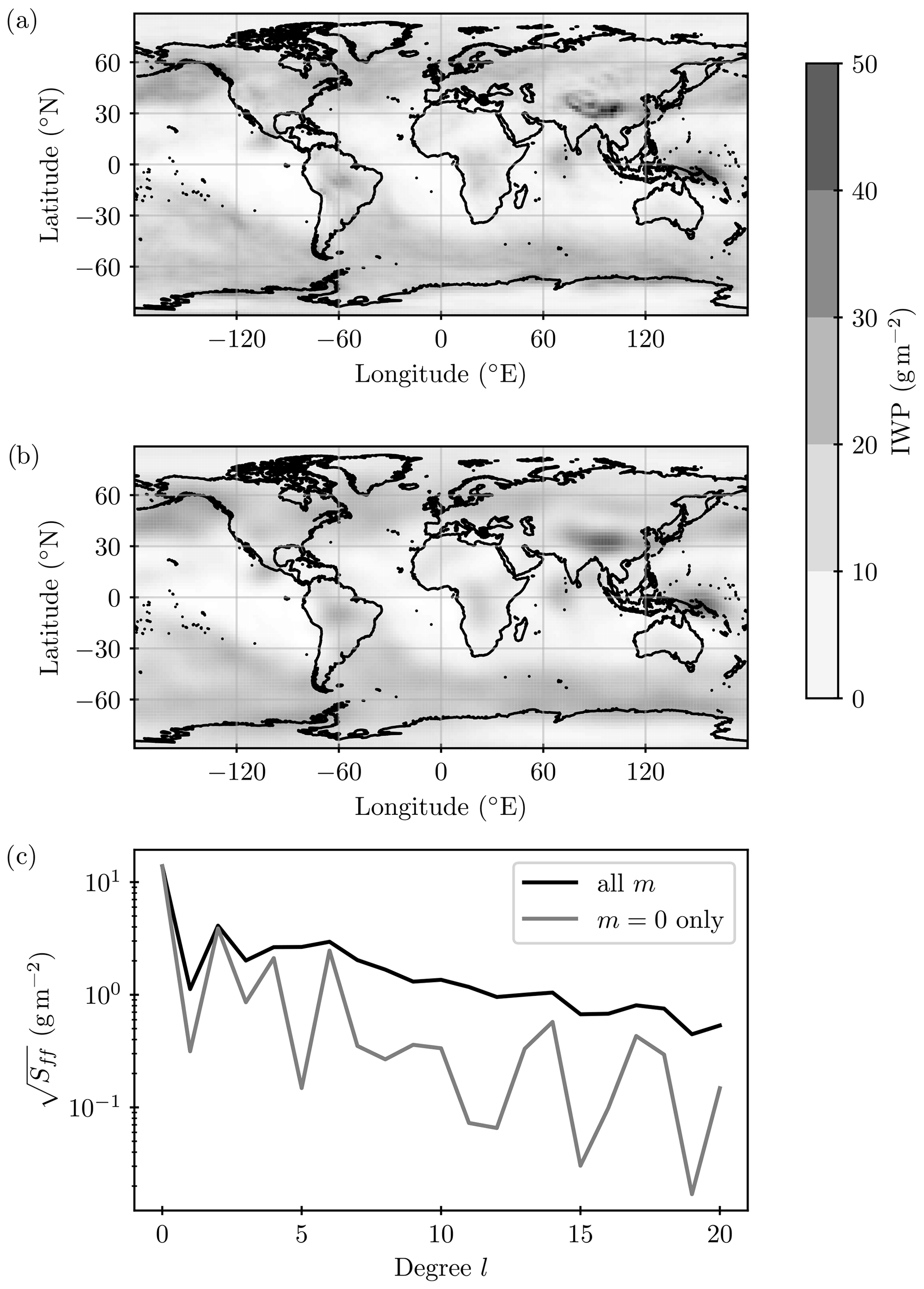
Figure 10Spherical harmonics expansions for one illustrative PPE member (ηautc≈0.87, ηaccr≈1.43, ηrime≈0.81, ηsci≈1.89). (a) Global annual mean IWP and (b) expansion of spherical harmonics representing the same data as (a), generated from the coefficients of the expansion displayed as an angular amplitude spectrum in (c) as a function of the degree l (with m independent solutions, where modes of m=0 most strongly resemble rotationally symmetric physical patterns of the Earth system such as a north–south contrast). Note that the variability explained by each degree l in general decreases with increasing l, which allows us to truncate the expansion at the degree l where it represents 95 % of the total data variance.
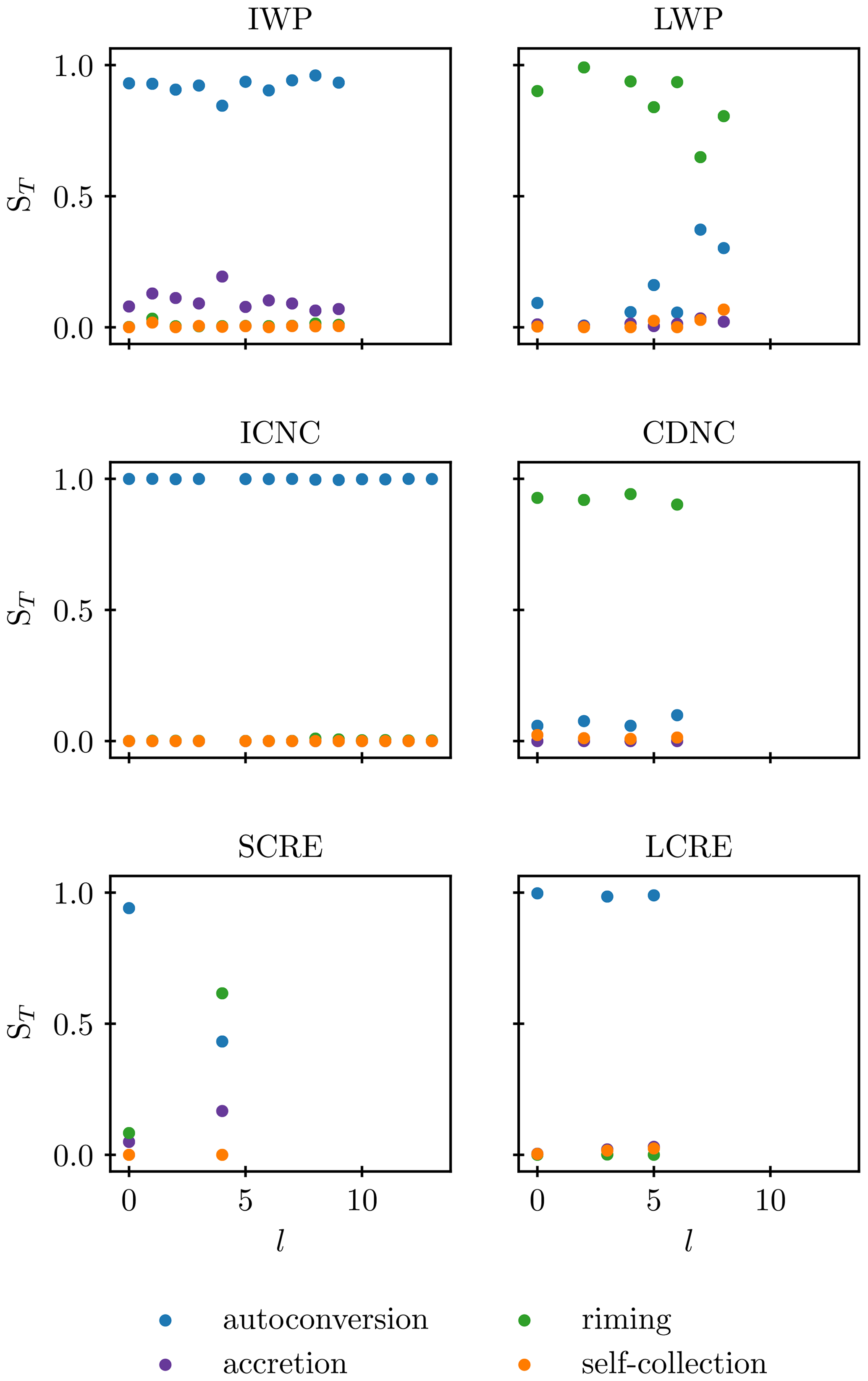
The results are displayed in Fig. 11. For those variables that had total sensitivity indices for autoconversion of over 0.9 (IWP, longwave cloud radiative effect, and ICNC) the dominant effect of autoconversion is present on all length scales. Accretion is of secondary importance for the IWP, as indicated by the global sensitivity analysis. The LWP and CDNC are dominated by riming on all regional scales and on the global scale.
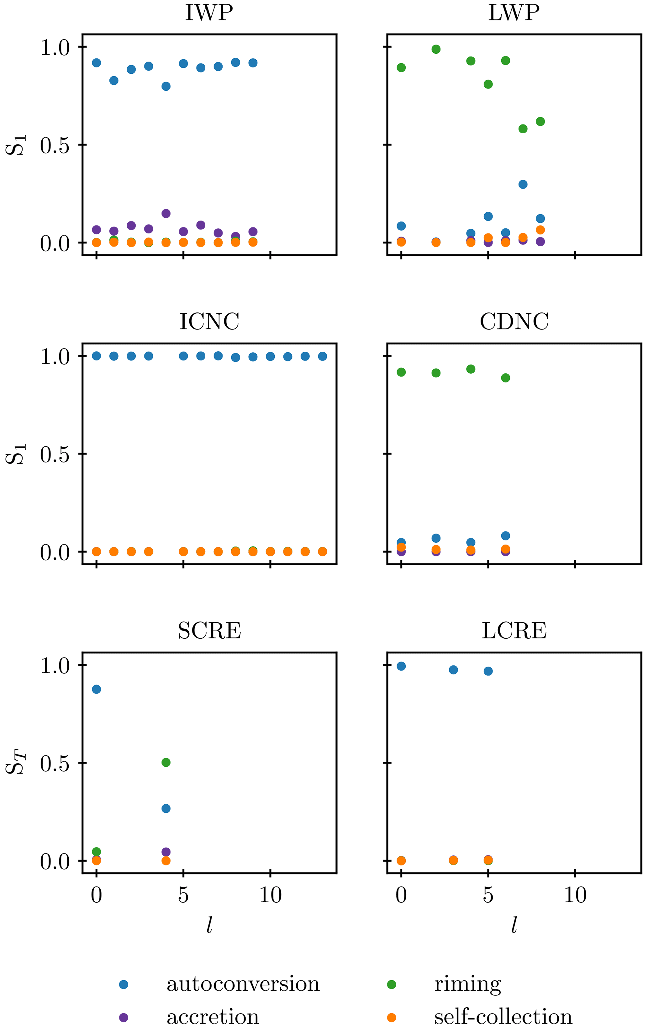
Figure 11First-order sensitivity indices for the emulated angular amplitude spectrum as a function of the spherical harmonics degree l for the variables as described for Fig. 9. As detailed in the text, emulators that were found to be defaulting in the validation procedure were not subjected to the sensitivity analysis so that the results for those l are missing here. The results for the total sensitivity index are shown in Fig. C1 in Appendix C.
The emulated surfaces for the spherical harmonics are more uncertain than those for the global mean values (see Appendix D). This is expected as the training data are more noisy and indicate a less detectable signal on smaller length scales than on the global one. In addition, the separate emulation for different degrees l ignores correlations between signals included in multiple degrees l, which may lead to the loss of signals that are small in the different l but correlated, and should therefore be addressed in future studies. However, as the results of the sensitivity analysis are clear in that variability is dominated by autoconversion (see Fig. 11), we can conclude that the results of the global sensitivity analysis also hold on regional scales.
Finally, this analysis demonstrates that spherical harmonics expansion is a viable tool to evaluate model output on all length scales in an efficient and objective manner. Future studies may use it to compare results, e.g., from different models. As most expansion degrees are physically difficult to interpret, the method may be expanded to use physically meaningful modes such as the land–sea contrast instead.
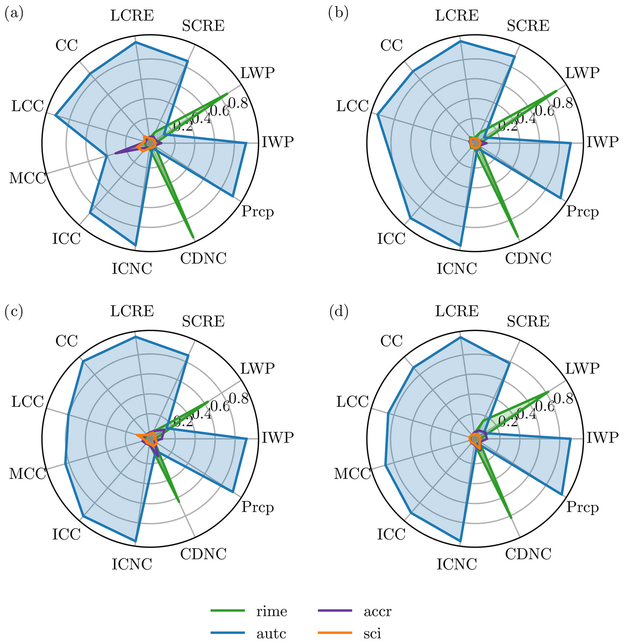
3.5 Seasonal analysis
Similar to a regional analysis, we use a temporally resolved sensitivity analysis to address the concern that conclusions drawn from annual mean values might not hold on a seasonal scale. Figure 12 shows the results of the same sensitivity analysis as in Fig. 9, but split by seasons (one emulator per variable was trained and validated for each season; note that in a few cases only 47 PPE members were used as with the 48th member the computational constraint was too tight for the emulator). Due to a weaker or less consistent signal in the data on seasonal scales, one variable (mixed-phase cloud cover in MAM) did not pass the validation procedure as the emulator was found to be defaulting (as described for the spherical harmonics above and in Appendix D). Figure 12 reveals that indeed the sensitivities to process perturbations are much the same as for the annual mean analysis. This confirms that the conclusions drawn for model simplifications also hold on a seasonal scale. The model is not sensitive to accretion and self-collection of ice, and therefore these processes can be simplified, while autoconversion and riming dominate the model response.
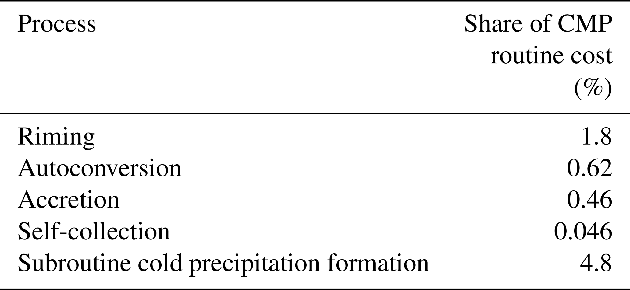
Table 1Share of the computing time taken up by the cloud microphysical processes investigated here. In turn, the CMP computing time represents 4.7 % of total computing time (excluding diagnostics; all values averaged over a 12-month control simulation with ). The time in the subroutine cold precipitation formation that is not attributed to the four processes is used for common initializations and subsequent processing.
3.6 Process costs and implications for simplification
The previous analysis shows that the response of ECHAM-HAM to a suppression of self-collection or accretion is negligible, while for riming and autoconversion a less accurate representation may be appropriate. A potential benefit could lie in the reduction of CPU time per model simulation. Table 1 lists the CPU time spent in the CMP routines of the four processes. The timings represent an estimate of how much time could be gained by removing a process from the model. They show that, at most, with naively removing (the most drastic simplification) the whole cold precipitation formation routine, only about 0.2 % of total computing time can be saved (since the cold precipitation formation routine makes up 4.8 % of the 4.7 % of computing time that the whole CMPs take up, see Table 1). In a 10-year simulation this would allow for 1 additional week of simulation, which is negligible in comparison to the computing needs of, e.g., increases in model resolution.
Within the CMP routine there are other physical processes that take up time, but the calculations of diagnostics and preparatory calculations also contribute. Of course, if numerous CMP processes and interactions with aerosols were simplified, this would allow for more drastic steps such as fewer prognostic aerosol variables as those could become redundant. Subsequently, significant reductions in model cost could be achieved. Yet by itself, the isolated removal or simplification of CMP processes provides small leverage for a decrease in computing time. However, as detailed in Sect. 1, there are numerous benefits in simplification that are independent of the associated computing cost, such as a gain in compactness and interpretability.
This study conducted a sensitivity analysis with an emulated PPE to illuminate the impact of selected CMP processes on model output. Different from previous studies (e.g., Wellmann et al., 2020; Hawker et al., 2021b), we perturb the four CMP processes of autoconversion, riming, accretion, and self-collection of ice as a whole. This is achieved by multiplying their process rates with a factor between 0.5 and 2. The resulting response surface of model output and its deviation from results with the default setup serve as a proxy for how accurately a process needs to be represented.
Perturbing only one process at a time reveals that ice crystal autoconversion acts as a threshold process: perturbing it causes the model to deviate, but when it is turned off the deviation is immense. This is because it is the only process that converts ice crystals to snow and as such accretion and riming depend on it. Using only roughly twice as many simulations as in the one-at-a-time perturbations to generate a PPE, we can generate the whole response surface using Gaussian process emulation. A sensitivity analysis of global and seasonal annual means reveals that for cloud cover, ice water path, and number concentration as well as shortwave and longwave radiative effect, the perturbation of autoconversion has the most dominant impact by far. Accretion and riming assume a secondary role. As riming is the only investigated process that directly affects the liquid phase, riming has a dominant effect on the liquid water path and cloud droplet number concentration. Self-collection of ice has a negligible impact on the investigated global annual mean variables. Resolving smaller horizontal scales using a spherical harmonics expansion of the output variables corroborates the results of the global annual mean analysis, as does a seasonal analysis. These results, as well as the shape of the response surface, suggest that the parameterization of self-collection and accretion can be readily and drastically simplified. While autoconversion and riming have a large impact on the model output considering the whole investigated phase space, the shallow slope of the response surface around the default ηi=1 hints that slight modifications of their representations may leave the model output unchanged. The strength of the PPE approach is that interactions are already taken into account, meaning that all four processes could be simplified at the same time. If one wants to develop the CMP scheme further, autoconversion is the process to scrutinize as it has the largest leverage in the model and therefore the most urgent need to be represented correctly.
As we find that the processes themselves use a negligible fraction of the overall model computing time, simplifications are proposed as a means to make the model more interpretable, not cheaper (see Sects. 1 and 3.6). Our analysis shows that the representation of the four investigated microphysical processes leaves room for simplification. However, in deciding how drastic these simplifications should be, process uncertainty should also be considered. At the least, when new parameterizations are included in climate models we should also question their implementation regarding the complexity they add, looking for their consistency, interpretability, simplicity, and comprehensiveness (Mülmenstädt and Feingold, 2018; Touzé-Pfeiffer et al., 2021). Of course, more drastic simplifications than process reformulations would provide more leverage on interpretability and computing cost. For example, CMP schemes that contain only one category for ice, e.g., the predicted particle properties (P3) ice microphysics scheme (e.g., Morrison and Milbrandt, 2015; Eidhammer et al., 2017; Dietlicher et al., 2018, 2019; Tully et al., 2021), are more physical as well as more interpretable. From this perspective it might seem troubling that in the current CMP scheme the autoconversion process, which is a transfer mechanism between the two artificial classes, is so dominant in its importance. However, while the categories are artificial, the process itself is not: accretion of ice crystals forming larger ice crystals would be the equivalent process with only one ice category. Still, autoconversion is also difficult to constrain in observations (Morrison et al., 2020) because it is not a distinct physical process, so moving towards a scheme with evolving instead of pre-defined ice categories seems advisable (see, e.g., Milbrandt and Morrison, 2016; Jensen et al., 2017).
This study introduces the methodological framework to study the sensitivity of a climate model to the representation of CMP processes. To complete it, the analysis needs to be expanded to include other CMP processes in the model: for cold CMP ice formation, regional modeling studies have demonstrated cloud susceptibility to the choice of the ice nucleation parameterization (Levkov et al., 1995; Hawker et al., 2021b), whereas in ECHAM-HAM heterogeneous immersion freezing in mixed-phase clouds has been shown to be rather inefficient (Villanueva et al., 2021). More generally the heterogeneous ice formation pathway in mixed-phase clouds is small in ECHAM-HAM (Dietlicher et al., 2019; Bacer et al., 2021), hinting at simplification potential. In a sensitivity study of CMP parameters, Tan and Storelvmo (2016) found that the timescale of the Wegener–Bergeron–Findeisen process explains a large variance in supercooled cloud fractions, suggesting that as a whole it may be a dominating process as well. Secondary ice formation (Korolev and Leisner, 2020) may interact with the ice crystal source processes, allowing for interactive sensitivities (Hawker et al., 2021b), and should therefore be included, even though only the Hallett–Mossop process is optionally included in ECHAM-HAM (Neubauer et al., 2019). Moreover, for a complete CMP process investigation, of course the warm-rain processes need to be included as well (Wood et al., 2009; Gettelman et al., 2013).
One might argue that our analysis neglects the influence of other factors external to the CMPs on our conclusions. However, as our simulations span the whole globe and a whole year, they cover a range of dynamical situations, and the results are therefore robust in the current climate. Whether the conclusions hold, e.g., in a future changed climate will have to be evaluated in a future study. It is important to stress that while we propose that simplifications to the CMP representation are possible, care needs to be taken to leave them physically based to ensure that the model can correctly represent differing climates. We emphasize that our findings are conditional on the design of the ECHAM-HAM model, including the implementation of other processes and parameters that were not varied in the current study. Another factor that has not been investigated here is the model resolution that may affect the CMP behavior in the model and thereby our conclusions on the importance of single processes (Santos et al., 2021). The implementation and design choices of the CMP scheme in ECHAM-HAM may also influence the results, e.g., in the order of processes that are called, the separation between ice and snow, and the employed tuning strategy. Thus, the results as such are only applicable to this CMP scheme and cannot be transferred to the significance of the investigated processes in other schemes let alone in reality.
Nevertheless, learning about the representation of CMP processes in ECHAM-HAM and how sensitive the model is to their representation helps us to interpret and improve the model, especially when comparing the results to experimental studies. To this end, it will also be fruitful to compare our findings to sensitivities in other models using different CMP schemes.
Table A1Tuning parameters that differ between this study and the reference of Neubauer et al. (2019). γr is the scaling factor for the stratiform rain formation rate by autoconversion. γs is a scaling factor for the stratiform snow formation rate by autoconversion. With the changes described in Sect. 2.1 the tuning parameter of the maximum cloud droplet radius, rCDNC, replaces the previous minimum cloud droplet number concentration, CDNCmin. The tuning parameter for immediate autoconversion of detrained ICNC, γd, is newly introduced.
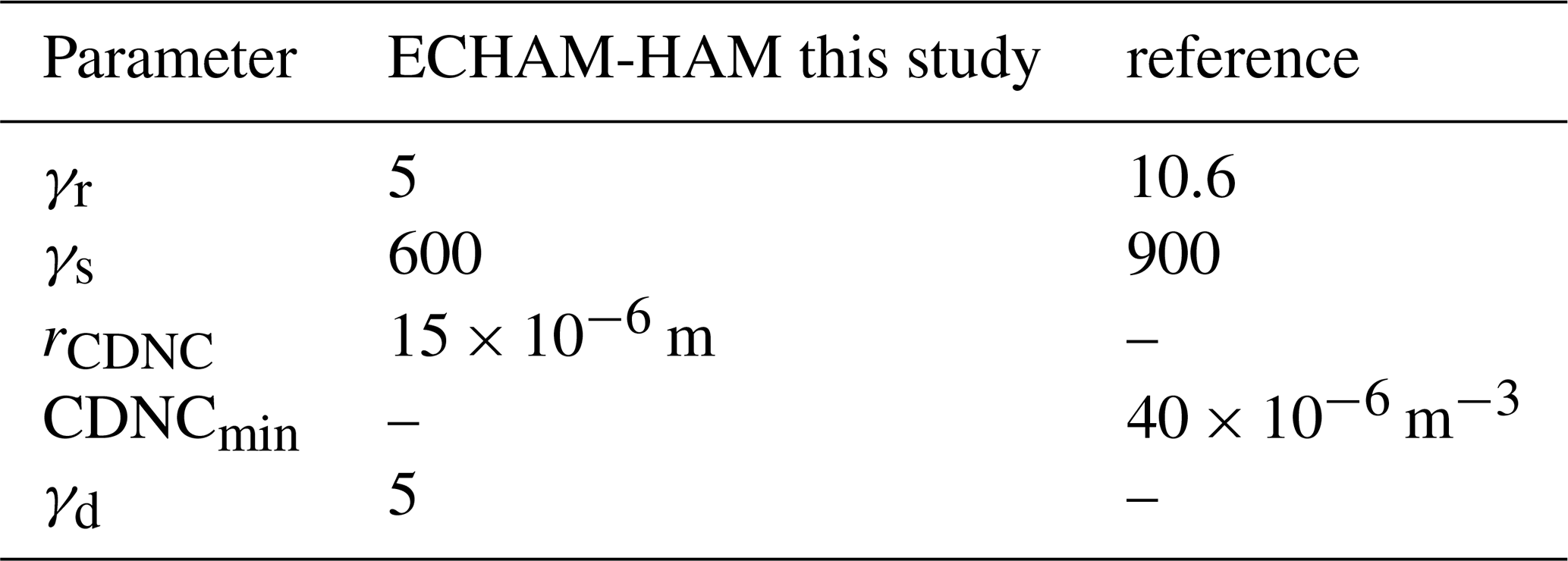
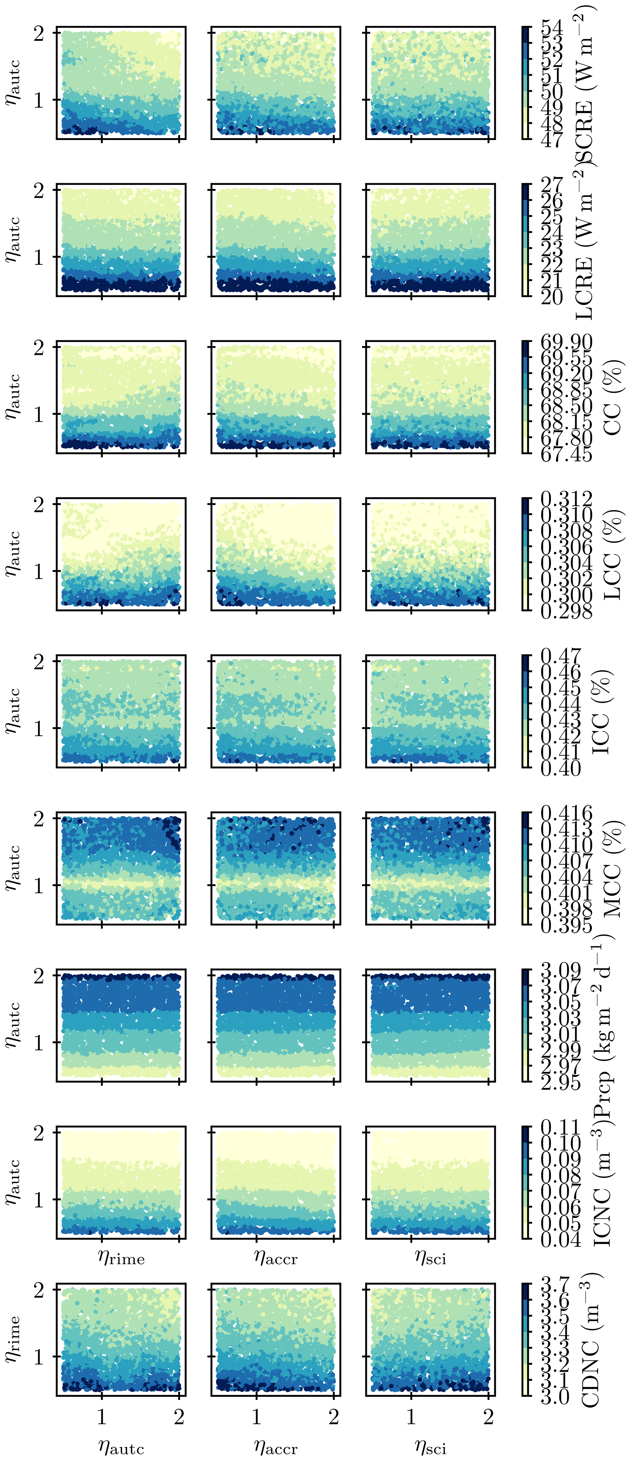
Figure B1Visualization of the multidimensional response surfaces of the emulated PPEs for multiple variables. Each process is a dimension, and the color bars denote the global annual mean values. In principle, each surface could be displayed by a full matrix plot as in Figs. 7 and 8, but here only the panels that include the dominating process are shown (autoconversion, except for CDNC in the last row, where riming is the dominant process).

The validation of the spherical harmonics emulation was carried out as described in Sect. 2.4. Larger uncertainties in the emulation were apparent for almost all variables and degrees l (see Fig. D1 for an example) than for the global mean values. However, some emulations were also found to be defaulting, meaning that they predicted a similar output value for the whole phase space (see Figs. D2 and D3 for an example). As this behavior points to a missing signal in the input, these points were excluded from further analysis if the following two criteria were not fulfilled (excluding the emulated outliers that are marked red, e.g., in Fig. 4).
-
The uncertainty in the prediction is smaller than the spread of the variable; i.e., the smallest error bar in Fig. D1d is smaller than 0.9ΔYsim.
-
The predictions are significantly different from each other; i.e., there is one pair of predictions whose error bars do not overlap.
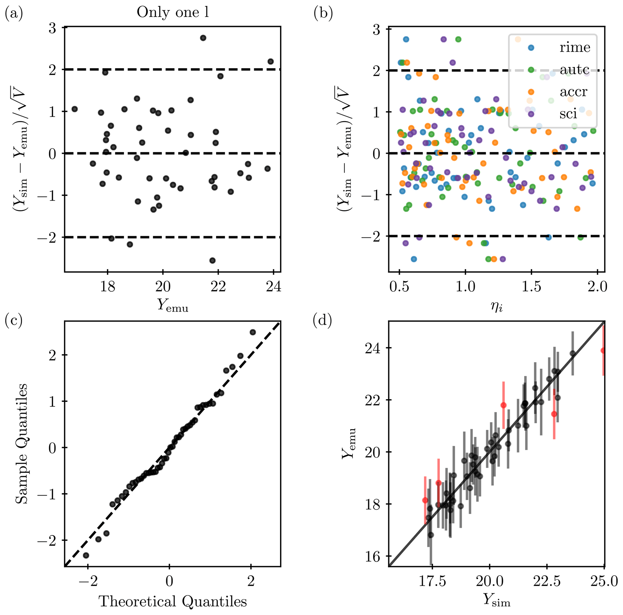

Figure D2Same as Fig. 7 but for the LWP spherical expansion angular amplitude spectrum of degree l=3. In this case, the emulator was found to be defaulting; it therefore failed the validation and was not included in the subsequent sensitivity analysis. The points enclosed by black circles denote the PPE member results used to train the emulator.
The ECHAM-HAMMOZ model is freely available to the scientific community under the HAMMOZ Software License Agreement, which defines the conditions under which the model can be used (https://redmine.hammoz.ethz.ch/projects/hammoz/wiki/2_How_to_get_the_sources, last access: 5 April 2022). The specific version of the code used for this study is archived in the ECHAM-HAMMOZ SVN repository at https://svn.iac.ethz.ch/external/echam-hammoz/echam6-hammoz/tags/papers/2022/Proske_et_al_2022_ACP_2 (last access: 25 February 2022). More information can be found on the HAMMOZ website (https://redmine.hammoz.ethz.ch/projects/hammoz, last access: 17 September 2021; HAMMOZ, 2022). Analysis and plotting scripts are archived at https://doi.org/10.5281/zenodo.5506588 (Proske et al., 2022). Generated data are archived at https://doi.org/10.5281/zenodo.5506533 (Proske et al., 2022). The PyDOE library (tisimst, 2021; https://github.com/tisimst/pyDOE, last access: 28 March 2022) was used for Latin hypercube sampling, ESEm was used (Watson-Parris and Williams, 2021, https://doi.org/10.5281/ZENODO.5196631; Watson-Parris et al., 2021, https://doi.org/10.5194/gmd-14-7659-2021) for the construction of the emulator, SALib (Usher et al., 2020; https://doi.org/10.5281/ZENODO.598306) was used for the sensitivity analysis, and PySphereX (Staab, 2021; https://doi.org/10.5281/ZENODO.5520635) was used for the construction of the spherical harmonics expansion.
UP developed the model code, ran the simulations and emulation, analyzed the data, and wrote the paper. UP, SF, DN, and UL developed the study idea and design and analyzed the results. MS and UP developed the idea for the spherical harmonics analysis, for which MS developed the code. SF, DN, UL, and MS edited the paper.
The contact author has declared that neither they nor their co-authors have any competing interests.
Publisher's note: Copernicus Publications remains neutral with regard to jurisdictional claims in published maps and institutional affiliations.
The authors thank Duncan Watson-Parris for his advice on using ESEm and helpful discussions. They are grateful to Rachel Hawker and Leighton Regayre for their advice on the emulation. The authors would like to thank the two reviewers for their careful and constructive feedback, which has improved this work substantially.
The ECHAM-HAMMOZ model is developed by a consortium composed of ETH Zurich, Max-Planck-Institut für Meteorologie, Forschungszentrum Jülich, University of Oxford, the Finnish Meteorological Institute, and the Leibniz Institute for Tropospheric Research; it is managed by the Leibniz Institute for Tropospheric Research (TROPOS). Throughout this study, the programming languages CDO (Schulzweida, 2019) and Python (Python Software Foundation, http://www.python.org, last access: 28 March 2022) were used to handle data and analyze them. Ulrike Proske, David Neubauer, and Ulrike Lohmann acknowledge support from the project FORCeS funded by Horizon H2020-EU.3.5.1.
This research has been supported by the European Commission, Horizon 2020 (FORCeS (grant no. 821205)).
This paper was edited by Graham Feingold and reviewed by two anonymous referees.
Adams, G. S.: People Systematically Overlook Subtractive Changes, Nature, 592, 17, https://doi.org/10.1038/s41586-021-03380-y, 2021. a
Archer-Nicholls, S., Abraham, N. L., Shin, Y. M., Weber, J., Russo, M. R., Lowe, D., Utembe, S. R., O'Connor, F. M., Kerridge, B., Latter, B., Siddans, R., Jenkin, M., Wild, O., and Archibald, A. T.: The Common Representative Intermediates Mechanism Version 2 in the United Kingdom Chemistry and Aerosols Model, J. Adv. Model. Earth Sy., 13, e2020MS002420, https://doi.org/10.1029/2020MS002420, 2021. a
Bacer, S., Sullivan, S. C., Sourdeval, O., Tost, H., Lelieveld, J., and Pozzer, A.: Cold cloud microphysical process rates in a global chemistry–climate model, Atmos. Chem. Phys., 21, 1485–1505, https://doi.org/10.5194/acp-21-1485-2021, 2021. a, b, c, d, e, f, g, h, i
Bastos, L. S. and O'Hagan, A.: Diagnostics for Gaussian Process Emulators, Technometrics, 51, 425–438, https://doi.org/10.1198/TECH.2009.08019, 2009. a, b, c, d
Bergeron, T.: On the Physics of Clouds and Precipitation, Proces Verbaux de l'Association de Météorologie, Paris, 156–178, 1935. a
Bernus, A., Ottlé, C., and Raoult, N.: Variance Based Sensitivity Analysis of FLake Lake Model for Global Land Surface Modeling, J. Geophys. Res.-Atmos., 126, e2019JD031928, https://doi.org/10.1029/2019JD031928, 2021. a
Beusch, L., Gudmundsson, L., and Seneviratne, S. I.: Emulating Earth system model temperatures with MESMER: from global mean temperature trajectories to grid-point-level realizations on land, Earth Syst. Dynam., 11, 139–159, https://doi.org/10.5194/esd-11-139-2020, 2020. a
Boucher, O., Randall, D., Artaxo, P., Bretherton, C., Feingold, G., Forster, P., Kerminen, V.-M., Kondo, Y., Liao, H., Lohmann, U., Rasch, P., Satheesh, S. K., Sherwood, S., Stevens, B., and Zhang, X. Y.: Clouds and Aerosols, in: Climate Change 2013: The Physical Science Basis. Contribution of Working Group I to the Fifth Assessment Report of the Intergovernmental Panel on Climate Change, Cambridge University Press, Cambridge, UK and New York, NY, USA, 2013. a
Carslaw, K., Lee, L., Regayre, L., and Johnson, J.: Climate Models Are Uncertain, but We Can Do Something About It, Eos, 99, https://doi.org/10.1029/2018EO093757, 2018. a
Carslaw, K. S., Lee, L. A., Reddington, C. L., Pringle, K. J., Rap, A., Forster, P. M., Mann, G. W., Spracklen, D. V., Woodhouse, M. T., Regayre, L. A., and Pierce, J. R.: Large Contribution of Natural Aerosols to Uncertainty in Indirect Forcing, Nature, 503, 67–71, https://doi.org/10.1038/nature12674, 2013. a, b
Cess, R. D., Potter, G. L., Blanchet, J. P., Boer, G. J., Del Genio, A. D., Déqué, M., Dymnikov, V., Galin, V., Gates, W. L., Ghan, S. J., Kiehl, J. T., Lacis, A. A., Le Treut, H., Li, Z.-X., Liang, X.-Z., McAvaney, B. J., Meleshko, V. P., Mitchell, J. F. B., Morcrette, J.-J., Randall, D. A., Rikus, L., Roeckner, E., Royer, J. F., Schlese, U., Sheinin, D. A., Slingo, A., Sokolov, A. P., Taylor, K. E., Washington, W. M., Wetherald, R. T., Yagai, I., and Zhang, M.-H.: Intercomparison and Interpretation of Climate Feedback Processes in 19 Atmospheric General Circulation Models, J. Geophys. Res., 95, 16601–16615, https://doi.org/10.1029/JD095iD10p16601, 1990. a
Collins, M., Booth, B. B. B., Bhaskaran, B., Harris, G. R., Murphy, J. M., Sexton, D. M. H., and Webb, M. J.: Climate Model Errors, Feedbacks and Forcings: A Comparison of Perturbed Physics and Multi-Model Ensembles, Clim. Dynam., 36, 1737–1766, https://doi.org/10.1007/s00382-010-0808-0, 2011. a
Couvreux, F., Hourdin, F., Williamson, D., Roehrig, R., Volodina, V., Villefranque, N., Rio, C., Audouin, O., Salter, J., Bazile, E., Brient, F., Favot, F., Honnert, R., Lefebvre, M.-P., Madeleine, J.-B., Rodier, Q., and Xu, W.: Process-Based Climate Model Development Harnessing Machine Learning: I. A Calibration Tool for Parameterization Improvement, J. Adv. Model. Earth Sy., 13, e2020MS002217, https://doi.org/10.1029/2020MS002217, 2021. a, b
Dagon, K., Sanderson, B. M., Fisher, R. A., and Lawrence, D. M.: A machine learning approach to emulation and biophysical parameter estimation with the Community Land Model, version 5, Adv. Stat. Clim. Meteorol. Oceanogr., 6, 223–244, https://doi.org/10.5194/ascmo-6-223-2020, 2020. a, b
Dietlicher, R., Neubauer, D., and Lohmann, U.: Prognostic parameterization of cloud ice with a single category in the aerosol-climate model ECHAM(v6.3.0)-HAM(v2.3), Geosci. Model Dev., 11, 1557–1576, https://doi.org/10.5194/gmd-11-1557-2018, 2018. a
Dietlicher, R., Neubauer, D., and Lohmann, U.: Elucidating ice formation pathways in the aerosol–climate model ECHAM6-HAM2, Atmos. Chem. Phys., 19, 9061–9080, https://doi.org/10.5194/acp-19-9061-2019, 2019. a, b, c, d
Duvenaud, D. K.: Automatic Model Construction with Gaussian Processes, PhD thesis, University of Cambridge, https://doi.org/10.17863/CAM.14087, 2014. a
Eidhammer, T., Morrison, H., Mitchell, D., Gettelman, A., and Erfani, E.: Improvements in Global Climate Model Microphysics Using a Consistent Representation of Ice Particle Properties, J. Climate, 30, 609–629, https://doi.org/10.1175/JCLI-D-16-0050.1, 2017. a
Errico, R. M.: What Is an Adjoint Model?, B. Am. Meteorol. Soc., 78, 16, 2577–2592, 1997. a
Findeisen, W.: Kolloid-Meteorologische Vorgänge Bei Neiderschlagsbildung, Meteorol. Z., 55, 121–133, 1938. a
Fisher, R. A. and Koven, C. D.: Perspectives on the Future of Land Surface Models and the Challenges of Representing Complex Terrestrial Systems, J. Adv. Model. Earth Sy., 12, e2018MS001453, https://doi.org/10.1029/2018MS001453, 2020. a, b, c
Friebel, F., Lobo, P., Neubauer, D., Lohmann, U., Drossaart van Dusseldorp, S., Mühlhofer, E., and Mensah, A. A.: Impact of isolated atmospheric aging processes on the cloud condensation nuclei activation of soot particles, Atmos. Chem. Phys., 19, 15545–15567, https://doi.org/10.5194/acp-19-15545-2019, 2019. a
Gasparini, B., Meyer, A., Neubauer, D., Münch, S., and Lohmann, U.: Cirrus Cloud Properties as Seen by the CALIPSO Satellite and ECHAM-HAM Global Climate Model, J. Climate, 31, 1983–2003, https://doi.org/10.1175/JCLI-D-16-0608.1, 2018. a
Gettelman, A., Morrison, H., Terai, C. R., and Wood, R.: Microphysical process rates and global aerosol–cloud interactions, Atmos. Chem. Phys., 13, 9855–9867, https://doi.org/10.5194/acp-13-9855-2013, 2013. a, b
Ghan, S. J., Liu, X., Easter, R. C., Zaveri, R., Rasch, P. J., Yoon, J.-H., and Eaton, B.: Toward a Minimal Representation of Aerosols in Climate Models: Comparative Decomposition of Aerosol Direct, Semidirect, and Indirect Radiative Forcing, J. Climate, 25, 6461–6476, https://doi.org/10.1175/JCLI-D-11-00650.1, 2012. a
Ghan, S. J., Smith, S. J., Wang, M., Zhang, K., Pringle, K., Carslaw, K., Pierce, J., Bauer, S., and Adams, P.: A Simple Model of Global Aerosol Indirect Effects, J. Geophys. Res.-Atmos., 118, 6688–6707, https://doi.org/10.1002/jgrd.50567, 2013. a, b
Glassmeier, F., Possner, A., Vogel, B., Vogel, H., and Lohmann, U.: A comparison of two chemistry and aerosol schemes on the regional scale and the resulting impact on radiative properties and liquid- and ice-phase aerosol–cloud interactions, Atmos. Chem. Phys., 17, 8651–8680, https://doi.org/10.5194/acp-17-8651-2017, 2017. a
Glassmeier, F., Hoffmann, F., Johnson, J. S., Yamaguchi, T., Carslaw, K. S., and Feingold, G.: An emulator approach to stratocumulus susceptibility, Atmos. Chem. Phys., 19, 10191–10203, https://doi.org/10.5194/acp-19-10191-2019, 2019. a
HAMMOZ: ECHAM-HAMMOZ, https://redmine.hammoz.ethz.ch/projects/hammoz, last access: 31 March 2022. a
Hawker, R. E., Miltenberger, A. K., Johnson, J. S., Wilkinson, J. M., Hill, A. A., Shipway, B. J., Field, P. R., Murray, B. J., and Carslaw, K. S.: Model emulation to understand the joint effects of ice-nucleating particles and secondary ice production on deep convective anvil cirrus, Atmos. Chem. Phys., 21, 17315–17343, https://doi.org/10.5194/acp-21-17315-2021, 2021a. a
Hawker, R. E., Miltenberger, A. K., Wilkinson, J. M., Hill, A. A., Shipway, B. J., Cui, Z., Cotton, R. J., Carslaw, K. S., Field, P. R., and Murray, B. J.: The temperature dependence of ice-nucleating particle concentrations affects the radiative properties of tropical convective cloud systems, Atmos. Chem. Phys., 21, 5439–5461, https://doi.org/10.5194/acp-21-5439-2021, 2021b. a, b, c
He, F. and Posselt, D. J.: Impact of Parameterized Physical Processes on Simulated Tropical Cyclone Characteristics in the Community Atmosphere Model, J. Climate, 28, 9857–9872, https://doi.org/10.1175/JCLI-D-15-0255.1, 2015. a
Herman, J. and Usher, W.: SALib: An Open-Source Python Library for Sensitivity Analysis, Journal of Open Source Software, 2, 97, https://doi.org/10.21105/joss.00097, 2017. a
Holden, P. B., Edwards, N. R., Garthwaite, P. H., and Wilkinson, R. D.: Emulation and Interpretation of High-Dimensional Climate Model Outputs, J. Appl. Stat., 42, 2038–2055, https://doi.org/10.1080/02664763.2015.1016412, 2015. a
Homma, T. and Saltelli, A.: Importance Measures in Global Sensitivity Analysis of Nonlinear Models, Reliab. Eng. Syst. Safe., 52, 1–17, https://doi.org/10.1016/0951-8320(96)00002-6, 1996. a
Hourdin, F., Williamson, D., Rio, C., Couvreux, F., Roehrig, R., Villefranque, N., Musat, I., Fairhead, L., Diallo, F. B., and Volodina, V.: Process-based Climate Model Development Harnessing Machine Learning: II. Model Calibration from Single Column to Global, J. Adv. Model. Earth Sy., 13, e2020MS002225, https://doi.org/10.1029/2020MS002225, 2020. a
Jensen, A. A., Harrington, J. Y., Morrison, H., and Milbrandt, J. A.: Predicting Ice Shape Evolution in a Bulk Microphysics Model, J. Atmos. Sci., 74, 2081–2104, https://doi.org/10.1175/JAS-D-16-0350.1, 2017. a
Johnson, J. S., Cui, Z., Lee, L. A., Gosling, J. P., Blyth, A. M., and Carslaw, K. S.: Evaluating Uncertainty in Convective Cloud Microphysics Using Statistical Emulation, J. Adv. Model. Earth Sy., 7, 162–187, https://doi.org/10.1002/2014MS000383, 2015. a, b, c, d
Johnson, J. S., Regayre, L. A., Yoshioka, M., Pringle, K. J., Lee, L. A., Sexton, D. M. H., Rostron, J. W., Booth, B. B. B., and Carslaw, K. S.: The importance of comprehensive parameter sampling and multiple observations for robust constraint of aerosol radiative forcing, Atmos. Chem. Phys., 18, 13031–13053, https://doi.org/10.5194/acp-18-13031-2018, 2018. a
Kärcher, B. and Lohmann, U.: A Parameterization of Cirrus Cloud Formation: Homogeneous Freezing of Supercooled Aerosols, J. Geophys. Res., 107, 4010, https://doi.org/10.1029/2001JD000470, 2002a. a
Kärcher, B. and Lohmann, U.: A Parameterization of Cirrus Cloud Formation: Homogeneous Freezing Including Effects of Aerosol Size: CIRRUS PARAMETERIZATION, J. Geophys. Res.-Atmos., 107, AAC 9–1–AAC 9–10, https://doi.org/10.1029/2001JD001429, 2002b. a
Knutti, R. and Sedláček, J.: Robustness and Uncertainties in the New CMIP5 Climate Model Projections, Nat. Clim. Change, 3, 369–373, https://doi.org/10.1038/nclimate1716, 2013. a, b
Koren, I. and Feingold, G.: Aerosol–Cloud–Precipitation System as a Predator-Prey Problem, P. Natl. Acad. Sci. USA, 108, 7, https://doi.org/10.1073/pnas.1101777108, 2011. a
Korolev, A. and Leisner, T.: Review of experimental studies of secondary ice production, Atmos. Chem. Phys., 20, 11767–11797, https://doi.org/10.5194/acp-20-11767-2020, 2020. a
Lee, L. A., Carslaw, K. S., Pringle, K. J., Mann, G. W., and Spracklen, D. V.: Emulation of a complex global aerosol model to quantify sensitivity to uncertain parameters, Atmos. Chem. Phys., 11, 12253–12273, https://doi.org/10.5194/acp-11-12253-2011, 2011. a, b, c, d, e
Lee, L. A., Carslaw, K. S., Pringle, K. J., and Mann, G. W.: Mapping the uncertainty in global CCN using emulation, Atmos. Chem. Phys., 12, 9739–9751, https://doi.org/10.5194/acp-12-9739-2012, 2012. a, b
Lee, L. A., Pringle, K. J., Reddington, C. L., Mann, G. W., Stier, P., Spracklen, D. V., Pierce, J. R., and Carslaw, K. S.: The magnitude and causes of uncertainty in global model simulations of cloud condensation nuclei, Atmos. Chem. Phys., 13, 8879–8914, https://doi.org/10.5194/acp-13-8879-2013, 2013. a
Lee, L. A., Reddington, C. L., and Carslaw, K. S.: On the Relationship between Aerosol Model Uncertainty and Radiative Forcing Uncertainty, P. Natl. Acad. Sci. USA, 113, 5820–5827, https://doi.org/10.1073/pnas.1507050113, 2016. a, b
Levkov, L., Boin, M., and Rockel, B.: Impact of Primary Ice Nucleation Parameterizations on the Formation and Maintenance of Cirrus, Atmos. Res., 38, 147–159, https://doi.org/10.1016/0169-8095(94)00091-Q, 1995. a
Liu, X., Easter, R. C., Ghan, S. J., Zaveri, R., Rasch, P., Shi, X., Lamarque, J.-F., Gettelman, A., Morrison, H., Vitt, F., Conley, A., Park, S., Neale, R., Hannay, C., Ekman, A. M. L., Hess, P., Mahowald, N., Collins, W., Iacono, M. J., Bretherton, C. S., Flanner, M. G., and Mitchell, D.: Toward a minimal representation of aerosols in climate models: description and evaluation in the Community Atmosphere Model CAM5, Geosci. Model Dev., 5, 709–739, https://doi.org/10.5194/gmd-5-709-2012, 2012. a
Loeppky, J. L., Sacks, J., and Welch, W. J.: Choosing the Sample Size of a Computer Experiment: A Practical Guide, Technometrics, 51, 366–376, https://doi.org/10.1198/TECH.2009.08040, 2009. a
Lohmann, U.: Possible Aerosol Effects on Ice Clouds via Contact Nucleation, J. Atmos. Sci., 59, 647–656, 2002. a, b
Lohmann, U.: Impact of the Mount Pinatubo Eruption on Cirrus Clouds Formed by Homogeneous Freezing in the ECHAM4 GCM, J. Geophys. Res., 108, 4568, https://doi.org/10.1029/2002JD003185, 2003. a
Lohmann, U. and Ferrachat, S.: Impact of parametric uncertainties on the present-day climate and on the anthropogenic aerosol effect, Atmos. Chem. Phys., 10, 11373–11383, https://doi.org/10.5194/acp-10-11373-2010, 2010. a, b, c
Lohmann, U. and Hoose, C.: Sensitivity studies of different aerosol indirect effects in mixed-phase clouds, Atmos. Chem. Phys., 9, 8917–8934, https://doi.org/10.5194/acp-9-8917-2009, 2009. a
Lohmann, U. and Neubauer, D.: The importance of mixed-phase and ice clouds for climate sensitivity in the global aerosol–climate model ECHAM6-HAM2, Atmos. Chem. Phys., 18, 8807–8828, https://doi.org/10.5194/acp-18-8807-2018, 2018. a, b
Lohmann, U. and Roeckner, E.: Design and Performance of a New Cloud Microphysics Scheme Developed for the ECHAM General Circulation Model, Clim. Dynam., 12, 557–572, 1996. a, b, c
Lohmann, U., Feichter, J., Chuang, C. C., and Penner, J. E.: Prediction of the Number of Cloud Droplets in the ECHAM GCM, J. Geophys. Res.-Atmos., 104, 9169–9198, https://doi.org/10.1029/1999JD900046, 1999. a, b
Lohmann, U., Stier, P., Hoose, C., Ferrachat, S., Kloster, S., Roeckner, E., and Zhang, J.: Cloud microphysics and aerosol indirect effects in the global climate model ECHAM5-HAM, Atmos. Chem. Phys., 7, 3425–3446, https://doi.org/10.5194/acp-7-3425-2007, 2007. a
Lohmann, U., Friebel, F., Kanji, Z. A., Mahrt, F., Mensah, A. A., and Neubauer, D.: Future Warming Exacerbated by Aged-Soot Effect on Cloud Formation, Nature Geosci., 13, 674–680, https://doi.org/10.1038/s41561-020-0631-0, 2020. a
Matus, A. V. and L'Ecuyer, T. S.: The Role of Cloud Phase in Earth's Radiation Budget, J. Geophys. Res.-Atmos., 122, 2559–2578, https://doi.org/10.1002/2016JD025951, 2017. a
McNeall, D., Williams, J., Booth, B., Betts, R., Challenor, P., Wiltshire, A., and Sexton, D.: The impact of structural error on parameter constraint in a climate model, Earth Syst. Dynam., 7, 917–935, https://doi.org/10.5194/esd-7-917-2016, 2016. a
Milbrandt, J. A. and Morrison, H.: Parameterization of Cloud Microphysics Based on the Prediction of Bulk Ice Particle Properties. Part III: Introduction of Multiple Free Categories, J. Atmos. Sci., 73, 975–995, https://doi.org/10.1175/JAS-D-15-0204.1, 2016. a
Morales, A., Posselt, D. J., and Morrison, H.: Which Combinations of Environmental Conditions and Microphysical Parameter Values Produce a Given Orographic Precipitation Distribution?, J. Atmos. Sci., 78, 619–638, https://doi.org/10.1175/JAS-D-20-0142.1, 2021. a
Morris, M. D. and Mitchell, T. J.: Exploratory Designs for Computational Experiments, J. Stat. Plan. Infer., 43, 381–402, 1995. a
Morrison, H. and Milbrandt, J. A.: Parameterization of Cloud Microphysics Based on the Prediction of Bulk Ice Particle Properties. Part I: Scheme Description and Idealized Tests, J. Atmos. Sci., 72, 287–311, https://doi.org/10.1175/JAS-D-14-0065.1, 2015. a
Morrison, H., Lier-Walqui, M., Fridlind, A. M., Grabowski, W. W., Harrington, J. Y., Hoose, C., Korolev, A., Kumjian, M. R., Milbrandt, J. A., Pawlowska, H., Posselt, D. J., Prat, O. P., Reimel, K. J., Shima, S.-I., Diedenhoven, B., and Xue, L.: Confronting the Challenge of Modeling Cloud and Precipitation Microphysics, J. Adv. Model. Earth Sy., 12, e2019MS001689, https://doi.org/10.1029/2019MS001689, 2020. a, b, c
Muench, S. and Lohmann, U.: Developing a Cloud Scheme With Prognostic Cloud Fraction and Two Moment Microphysics for ECHAM-HAM, J. Adv. Model. Earth Sy., 12, e2019MS001824, https://doi.org/10.1029/2019MS001824, 2020. a, b
Mulholland, D. P., Haines, K., Sparrow, S. N., and Wallom, D.: Climate Model Forecast Biases Assessed with a Perturbed Physics Ensemble, Clim. Dynam., 49, 1729–1746, https://doi.org/10.1007/s00382-016-3407-x, 2017. a
Mülmenstädt, J. and Feingold, G.: The Radiative Forcing of Aerosol–Cloud Interactions in Liquid Clouds: Wrestling and Embracing Uncertainty, Current Climate Change Reports, 4, 23–40, https://doi.org/10.1007/s40641-018-0089-y, 2018. a, b, c, d
Mülmenstädt, J., Sourdeval, O., Delanoë, J., and Quaas, J.: Frequency of Occurrence of Rain from Liquid-, Mixed-, and Ice-Phase Clouds Derived from A-Train Satellite Retrievals: Rain From Liquid- and Ice-Phase Clouds, Geophys. Res. Lett., 42, 6502–6509, https://doi.org/10.1002/2015GL064604, 2015. a
Murphy, J. M., Sexton, D. M. H., Barnett, D. N., Jones, G. S., Webb, M. J., Collins, M., and Stainforth, D. A.: Quantification of Modelling Uncertainties in a Large Ensemble of Climate Change Simulations, Nature, 430, 768–772, https://doi.org/10.1038/nature02771, 2004. a
Neubauer, D., Ferrachat, S., Siegenthaler-Le Drian, C., Stier, P., Partridge, D. G., Tegen, I., Bey, I., Stanelle, T., Kokkola, H., and Lohmann, U.: The global aerosol–climate model ECHAM6.3–HAM2.3 – Part 2: Cloud evaluation, aerosol radiative forcing, and climate sensitivity, Geosci. Model Dev., 12, 3609–3639, https://doi.org/10.5194/gmd-12-3609-2019, 2019. a, b, c, d, e, f, g, h, i
Oakley, J. E. and O'Hagan, A.: Probabilistic Sensitivity Analysis of Complex Models: A Bayesian Approach, J. R. Stat. Soc. B, 66, 751–769, https://doi.org/10.1111/j.1467-9868.2004.05304.x, 2004. a
O'Hagan, A.: Bayesian Analysis of Computer Code Outputs: A Tutorial, Reliab. Eng. Syst. Safe., 91, 1290–1300, https://doi.org/10.1016/j.ress.2005.11.025, 2006. a
Posselt, D. J.: A Bayesian Examination of Deep Convective Squall-Line Sensitivity to Changes in Cloud Microphysical Parameters, J. Atmos. Sci., 73, 637–665, https://doi.org/10.1175/JAS-D-15-0159.1, 2016. a
Proske, U., Ferrachat, S., Neubauer, D., Staab, M., and Lohmann, U.: Scripts for the publication “Assessing the potential for simplification in global climate model cloud microphysics”, Version 1.3, Zenodo [code], https://doi.org/10.5281/zenodo.6425241, 2022. a
Proske, U., Ferrachat, S., Neubauer, D., Staab, M., and Lohmann, U.: Data for the publication “Assessing the potential for simplification in global climate model cloud microphysics”, Version 1.3, Zenodo [data set], https://doi.org/10.5281/zenodo.6326950, 2022. a
Qian, Y., Jackson, C., Giorgi, F., Booth, B., Duan, Q., Forest, C., Higdon, D., Hou, Z. J., and Huerta, G.: Uncertainty Quantification in Climate Modeling and Projection, B. Am. Meteorol. Soc., 97, 821–824, https://doi.org/10.1175/BAMS-D-15-00297.1, 2016. a
Rasmussen, C. E. and Williams, C. K. I.: Gaussian Processes for Machine Learning, Adaptive Computation and Machine Learning, MIT Press, Cambridge, Mass, 2006. a
Reddington, C. L., Carslaw, K. S., Stier, P., Schutgens, N., Coe, H., Liu, D., Allan, J., Browse, J., Pringle, K. J., Lee, L. A., Yoshioka, M., Johnson, J. S., Regayre, L. A., Spracklen, D. V., Mann, G. W., Clarke, A., Hermann, M., Henning, S., Wex, H., Kristensen, T. B., Leaitch, W. R., Pöschl, U., Rose, D., Andreae, M. O., Schmale, J., Kondo, Y., Oshima, N., Schwarz, J. P., Nenes, A., Anderson, B., Roberts, G. C., Snider, J. R., Leck, C., Quinn, P. K., Chi, X., Ding, A., Jimenez, J. L., and Zhang, Q.: The Global Aerosol Synthesis and Science Project (GASSP): Measurements and Modeling to Reduce Uncertainty, B. Am. Meteorol. Soc., 98, 1857–1877, https://doi.org/10.1175/BAMS-D-15-00317.1, 2017. a, b
Regayre, L. A., Pringle, K. J., Booth, B. B. B., Lee, L. A., Mann, G. W., Browse, J., Woodhouse, M. T., Rap, A., Reddington, C. L., and Carslaw, K. S.: Uncertainty in the Magnitude of Aerosol-Cloud Radiative Forcing over Recent Decades, Geophys. Res. Lett., 41, 9040–9049, https://doi.org/10.1002/2014GL062029, 2014. a
Regayre, L. A., Pringle, K. J., Lee, L. A., Rap, A., Browse, J., Mann, G. W., Reddington, C. L., Carslaw, K. S., Booth, B. B. B., and Woodhouse, M. T.: The Climatic Importance of Uncertainties in Regional Aerosol–Cloud Radiative Forcings over Recent Decades, J. Climate, 28, 6589–6607, https://doi.org/10.1175/JCLI-D-15-0127.1, 2015. a
Regayre, L. A., Johnson, J. S., Yoshioka, M., Pringle, K. J., Sexton, D. M. H., Booth, B. B. B., Lee, L. A., Bellouin, N., and Carslaw, K. S.: Aerosol and physical atmosphere model parameters are both important sources of uncertainty in aerosol ERF, Atmos. Chem. Phys., 18, 9975–10006, https://doi.org/10.5194/acp-18-9975-2018, 2018. a, b
Rougier, J., Sexton, D. M. H., Murphy, J. M., and Stainforth, D.: Analyzing the Climate Sensitivity of the HadSM3 Climate Model Using Ensembles from Different but Related Experiments, J. Climate, 22, 3540–3557, https://doi.org/10.1175/2008JCLI2533.1, 2009. a, b
Rudin, C.: Stop Explaining Black Box Machine Learning Models for High Stakes Decisions and Use Interpretable Models Instead, Nature Machine Intelligence, 1, 206–215, https://doi.org/10.1038/s42256-019-0048-x, 2019. a
Ryan, E., Wild, O., Voulgarakis, A., and Lee, L.: Fast sensitivity analysis methods for computationally expensive models with multi-dimensional output, Geosci. Model Dev., 11, 3131–3146, https://doi.org/10.5194/gmd-11-3131-2018, 2018. a
Saltelli, A. (Ed.): Global Sensitivity Analysis: The Primer, John Wiley, Chichester, England, Hoboken, NJ, 2008. a, b
Saltelli, A., Tarantola, S., and Chan, K. P.-S.: A Quantitative Model-Independent Method for Global Sensitivity Analysis of Model Output, Technometrics, 41, 39–56, https://doi.org/10.1080/00401706.1999.10485594, 1999. a
Santos, S. P., Caldwell, P. M., and Bretherton, C. S.: Cloud Process Coupling and Time Integration in the E3SM Atmosphere Model, J. Adv. Model. Earth Sy., 13, e2020MS002359, https://doi.org/10.1029/2020MS002359, 2021. a
Schulzweida, U.: CDO User Guide, Version 1.9.8, Zenodo, https://doi.org/10.5281/zenodo.3539275, 2019. a
Schutgens, N. A. J. and Stier, P.: A pathway analysis of global aerosol processes, Atmos. Chem. Phys., 14, 11657–11686, https://doi.org/10.5194/acp-14-11657-2014, 2014. a
Seifert, A. and Rasp, S.: Potential and Limitations of Machine Learning for Modeling Warm-Rain Cloud Microphysical Processes, J. Adv. Model. Earth Sy., 12, e2020MS002301, https://doi.org/10.1029/2020MS002301, 2020. a
Sengupta, K., Pringle, K., Johnson, J. S., Reddington, C., Browse, J., Scott, C. E., and Carslaw, K.: A global model perturbed parameter ensemble study of secondary organic aerosol formation, Atmos. Chem. Phys., 21, 2693–2723, https://doi.org/10.5194/acp-21-2693-2021, 2021. a
Soden, B. J. and Held, I. M.: An Assessment of Climate Feedbacks in Coupled Ocean-Atmosphere Models, J. Climate, 19, 3354–3360, https://doi.org/10.1175/JCLI3799.1, 2006. a
Sotiropoulou, G., Vignon, É., Young, G., Morrison, H., O'Shea, S. J., Lachlan-Cope, T., Berne, A., and Nenes, A.: Secondary ice production in summer clouds over the Antarctic coast: an underappreciated process in atmospheric models, Atmos. Chem. Phys., 21, 755–771, https://doi.org/10.5194/acp-21-755-2021, 2021. a
Staab, M.: marstaa/PySphereX: v1.0, Version v1.0, Zenodo [code], https://doi.org/10.5281/zenodo.5520636, 2021. a
Storelvmo, T., Kristjánsson, J. E., Lohmann, U., Iversen, T., Kirkevåg, A., and Seland, Ø.: Modeling of the Wegener–Bergeron–Findeisen Process—Implications for Aerosol Indirect Effects, Environ. Res. Lett., 3, 045001, https://doi.org/10.1088/1748-9326/3/4/045001, 2008. a
Sun, Z. and Shine, K. P.: Parameterization of Ice Cloud Radiative Properties and Its Application to the Potential Climatic Importance of Mixed-Phase Clouds, J. Climate, 8, 1874–1888, https://doi.org/10.1175/1520-0442(1995)008<1874:POICRP>2.0.CO;2, 1995. a
Tan, I. and Storelvmo, T.: Sensitivity Study on the Influence of Cloud Microphysical Parameters on Mixed-Phase Cloud Thermodynamic Phase Partitioning in CAM5, J. Atmos. Sci., 73, 709–728, https://doi.org/10.1175/JAS-D-15-0152.1, 2016. a, b
Tan, I., Storelvmo, T., and Zelinka, M. D.: Observational Constraints on Mixed-Phase Clouds Imply Higher Climate Sensitivity, Science, 352, 224–227, https://doi.org/10.1126/science.aad5300, 2016. a
Tegen, I., Neubauer, D., Ferrachat, S., Siegenthaler-Le Drian, C., Bey, I., Schutgens, N., Stier, P., Watson-Parris, D., Stanelle, T., Schmidt, H., Rast, S., Kokkola, H., Schultz, M., Schroeder, S., Daskalakis, N., Barthel, S., Heinold, B., and Lohmann, U.: The global aerosol–climate model ECHAM6.3–HAM2.3 – Part 1: Aerosol evaluation, Geosci. Model Dev., 12, 1643–1677, https://doi.org/10.5194/gmd-12-1643-2019, 2019. a
Tett, S. F. B., Rowlands, D. J., Mineter, M. J., and Cartis, C.: Can Top-of-Atmosphere Radiation Measurements Constrain Climate Predictions? Part II: Climate Sensitivity, J. Climate, 26, 9367–9383, https://doi.org/10.1175/JCLI-D-12-00596.1, 2013. a
tisimst: PyDOE: The Experimental Design Package for Python, https://github.com/tisimst/pyDOE (last access: 28 March 2022), 2021. a, b
Touzé-Pfeiffer, L., Hourdin, F., and Rio, C.: Parameterization and Tuning of Cloud and Precipitation Overlap in LMDz, in: Improvement and Calibration of Clouds in Models, Conference Presentation, Toulouse, France, 12–16 April 2021, http://www.meteo.fr/cic/meetings/2021/high-tune/documents.html (last access: 28 March 2022), 2021. a
Tully, C., Neubauer, D., Omanovic, N., and Lohmann, U.: Cirrus cloud thinning using a more physically-based ice microphysics scheme in the ECHAM-HAM GCM, Atmos. Chem. Phys. Discuss. [preprint], https://doi.org/10.5194/acp-2021-685, in review, 2021. a
Usher, W., Herman, J., Iwanaga, T., Teixeira, L., Cellier, N., Whealton, C., Hadka, D., xantares, bernardoct, Rios, F., Mutel, C., Cederstrand, E., TobiasKAndersen, van Engelen, J., ANtlord, Kranas, H., Dixit, V. K., and bsteubing: SALib/SALib: Public Beta, Zenodo [code], https://doi.org/10.5281/ZENODO.598306, 2020. a
van Lier-Walqui, M., Vukicevic, T., and Posselt, D. J.: Linearization of Microphysical Parameterization Uncertainty Using Multiplicative Process Perturbation Parameters, Mon. Weather Rev., 142, 401–413, https://doi.org/10.1175/MWR-D-13-00076.1, 2014. a, b
van Lier-Walqui, M., Morrison, H., Kumjian, M. R., Reimel, K. J., Prat, O. P., Lunderman, S., and Morzfeld, M.: A Bayesian Approach for Statistical–Physical Bulk Parameterization of Rain Microphysics. Part II: Idealized Markov Chain Monte Carlo Experiments, J. Atmos. Sci., 77, 1043–1064, https://doi.org/10.1175/JAS-D-19-0071.1, 2019. a
Villanueva, D., Neubauer, D., Gasparini, B., Ickes, L., and Tegen, I.: Constraining the Impact of Dust-Driven Droplet Freezing on Climate Using Cloud-Top-Phase Observations, Geophys. Res. Lett., 48, e2021GL092687, https://doi.org/10.1029/2021GL092687, 2021. a
Wacker, U.: Competition of Precipitation Particles in a Model with Parameterized Cloud Microphysics, J. Atmos. Sci., 52, 2577–89, 1995. a
Watson-Parris, D. and Williams, A.: duncanwp/ESEm: v1.0.0, Version v1.0.0, Zenodo [code], https://doi.org/10.5281/zenodo.5196632, 2021. a, b, c
Watson-Parris, D., Williams, A., Deaconu, L., and Stier, P.: Model calibration using ESEm v1.1.0 – an open, scalable Earth system emulator, Geosci. Model Dev., 14, 7659–7672, https://doi.org/10.5194/gmd-14-7659-2021, 2021. a, b, c, d
Wegener, A.: Thermodynamik der Atmosphäre, J. A. Barth, Leipzig, 1911. a
Wellmann, C., Barrett, A. I., Johnson, J. S., Kunz, M., Vogel, B., Carslaw, K. S., and Hoose, C.: Using Emulators to Understand the Sensitivity of Deep Convective Clouds and Hail to Environmental Conditions, J. Adv. Model. Earth Sy., 10, 3103–3122, https://doi.org/10.1029/2018MS001465, 2018. a, b
Wellmann, C., Barrett, A. I., Johnson, J. S., Kunz, M., Vogel, B., Carslaw, K. S., and Hoose, C.: Comparing the impact of environmental conditions and microphysics on the forecast uncertainty of deep convective clouds and hail, Atmos. Chem. Phys., 20, 2201–2219, https://doi.org/10.5194/acp-20-2201-2020, 2020. a, b, c, d
White, B., Gryspeerdt, E., Stier, P., Morrison, H., Thompson, G., and Kipling, Z.: Uncertainty from the choice of microphysics scheme in convection-permitting models significantly exceeds aerosol effects, Atmos. Chem. Phys., 17, 12145–12175, https://doi.org/10.5194/acp-17-12145-2017, 2017. a
Williams, K. D. and Tselioudis, G.: GCM Intercomparison of Global Cloud Regimes: Present-Day Evaluation and Climate Change Response, Clim. Dynam., 29, 231–250, https://doi.org/10.1007/s00382-007-0232-2, 2007. a
Williamson, D., Goldstein, M., Allison, L., Blaker, A., Challenor, P., Jackson, L., and Yamazaki, K.: History Matching for Exploring and Reducing Climate Model Parameter Space Using Observations and a Large Perturbed Physics Ensemble, Clim. Dynam., 41, 1703–1729, https://doi.org/10.1007/s00382-013-1896-4, 2013. a
Williamson, D., Blaker, A. T., Hampton, C., and Salter, J.: Identifying and Removing Structural Biases in Climate Models with History Matching, Clim. Dynam., 45, 1299–1324, https://doi.org/10.1007/s00382-014-2378-z, 2015. a, b
Wood, R., Kubar, T. L., and Hartmann, D. L.: Understanding the Importance of Microphysics and Macrophysics for Warm Rain in Marine Low Clouds. Part II: Heuristic Models of Rain Formation, J. Atmos. Sci., 66, 2973–2990, https://doi.org/10.1175/2009JAS3072.1, 2009. a, b
Yan, H., Qian, Y., Zhao, C., Wang, H., Wang, M., Yang, B., Liu, X., and Fu, Q.: A New Approach to Modeling Aerosol Effects on East Asian Climate: Parametric Uncertainties Associated with Emissions, Cloud Microphysics, and Their Interactions, J. Geophys. Res.-Atmos., 120, 8905–8924, https://doi.org/10.1002/2015JD023442, 2015. a, b
- Abstract
- Introduction
- Methods
- Results and discussion
- Summary, conclusions, and outlook
- Appendix A: Tuning
- Appendix B: PPE results for more variables
- Appendix C: Total sensitivity index
- Appendix D: Validation of the spherical harmonics sensitivity analysis
- Code and data availability
- Author contributions
- Competing interests
- Disclaimer
- Acknowledgements
- Financial support
- Review statement
- References