the Creative Commons Attribution 4.0 License.
the Creative Commons Attribution 4.0 License.
 | 07 Apr 2022
Technical note: Parameterising cloud base updraft velocity of marine stratocumuli
Jaakko Ahola
Muzaffer Ege Alper
Jukka-Pekka Keskinen
Harri Kokkola
Antti Kukkurainen
Antti Lipponen
Jia Liu
Kalle Nordling
Antti-Ilari Partanen
Sami Romakkaniemi
Petri Räisänen
Juha Tonttila
Hannele Korhonen
The number of cloud droplets formed at the cloud base depends on both the properties of aerosol particles and the updraft velocity of an air parcel at the cloud base. As the spatial scale of updrafts is too small to be resolved in global atmospheric models, the updraft velocity is commonly parameterised based on the available turbulent kinetic energy. Here we present alternative methods through parameterising updraft velocity based on high-resolution large-eddy simulation (LES) runs in the case of marine stratocumulus clouds. First we use our simulations to assess the accuracy of a simple linear parameterisation where the updraft velocity depends only on cloud top radiative cooling. In addition, we present two different machine learning methods (Gaussian process emulation and random forest) that account for different boundary layer conditions and cloud properties. We conclude that both machine learning parameterisations reproduce the LES-based updraft velocities at about the same accuracy, while the simple approach employing radiative cooling only produces on average lower coefficient of determination and higher root mean square error values. Finally, we apply these machine learning methods to find the key parameters affecting cloud base updraft velocities.
- Article
(4276 KB) - Full-text XML
-
Supplement
(503 KB) - BibTeX
- EndNote


Clouds are important for the global climate due to their ability to reflect solar radiation (short-wave radiation) and trap outgoing long-wave infrared radiation, but there are still several unknowns and uncertainties related to their dynamics including aerosol–cloud interactions (e.g. Wood, 2012; Seinfeld et al., 2016; Schneider et al., 2017; Rosenfeld et al., 2019). Cloud formation requires supersaturation with respect to water vapour and aerosol particles that can act as cloud condensation nuclei (CCN). Although several processes can lead to the formation of supersaturation within an air parcel, the most important one is the adiabatic cooling caused by updrafts. Malavelle et al. (2014) state that updraft velocities strongly control the activation of aerosol particles. Together with aerosol properties and concentrations, the strength of updraft determines the number of droplets formed. Cloud droplet number concentration (CDNC) directly impacts both the precipitation formation and the radiative properties of clouds.
The relative importance of aerosol properties and updraft speed for droplet concentration and aerosol indirect effects has been widely studied and found to be dependent on cloud type and aerosol loading (e.g. Lance et al., 2004; McFiggans et al., 2006; Reutter et al., 2009; Bougiatioti et al., 2020). Sullivan et al. (2016) state that input updraft velocity fluctuations can explain as much as 61 % of droplet number variability in GEOS-5. Kacarab et al. (2020) found that the characteristic vertical velocity (w*) plays a very important role in driving droplet formation in a rather polluted marine boundary layer (MBL) regime, in which even a small shift in w* may make a significant difference in droplet concentrations. Regayre et al. (2018) stated that vertical velocity standard deviation perturbations have the greatest influence on cloud droplet concentrations in regions of relatively high aerosol concentrations because in such environments droplet activation is updraft-limited rather than aerosol-limited. On a global scale, Yoshioka et al. (2019) found the uncertainty in the updraft velocity to be the second most important cause for uncertainty in aerosol radiative forcing.
Globally, shallow marine clouds have significant climate impacts because they cover major parts of oceans (Bennartz, 2007). At the same time, these clouds are particularly difficult to model because they require a high model resolution to capture the turbulence (Honnert et al., 2020). Such a resolution is available, for example, by using large-eddy simulation (LES). These models solve large turbulent eddies explicitly, and the smallest eddies are parameterised (e.g. Schneider et al., 2017). LES models are currently widely used and offer a good dynamical core and basis for cloud model development.
The resolution of cloud processes in a global model can be increased through the use of LES or cloud-resolving models (CRMs) in each general circulation model (GCM) column, which is known as superparameterisation (e.g. Khairoutdinov and Randall, 2001; Khairoutdinov et al., 2005). However, this is a computationally very demanding solution, so parameterisations are commonly used.
As the resolution of global atmospheric models is too coarse to resolve the cloud-scale updrafts, different parameterisations are employed to estimate either the probability density function of updrafts or a single characteristic updraft for the whole cloud. Most global models employ information on resolved turbulent kinetic energy or eddy diffusivity to parameterise the subgrid turbulence, which can be related to updraft velocity (Golaz et al., 2011). Other suggested methods, given in remote sensing studies (Zheng and Rosenfeld, 2015; Zheng et al., 2016), rely on parameterising the updraft based on the boundary layer properties and the forcing causing the turbulence. Zheng et al. (2016) stated that the parameterisation of vertical velocity has long been recognised as a core issue in numerical weather prediction. For example, it has been suggested that updraft depends on the cloud top radiative cooling in the case of stratocumulus (Zheng et al., 2016) or cloud base height for cumulus clouds (Zheng and Rosenfeld, 2015). Recently, machine learning approaches have gained attention because they can be used as parameterisations with higher accuracy than traditional parameterisations and with much smaller computational costs compared to explicit simulations (e.g. Rasp et al., 2018; Silva et al., 2021; Kashinath et al., 2021).
Here, we present three LES-based boundary layer cloud updraft velocity parameterisations that could be used within a global climate model. The parameterisations are based on detailed LES runs. The three methods are based on (1) a Gaussian process emulator, (2) a linear parameterisation based on cloud radiative cooling (Zheng et al., 2016) and (3) machine learning to correct the approximation error of the linear fit obtained with method 2 (Lipponen et al., 2013, 2018). We also examine which parameters are most important for predicting updraft velocities.
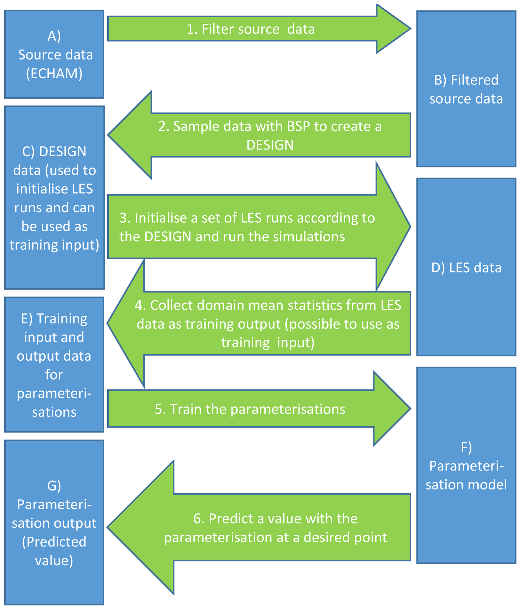
The parameterisations are specifically designed for marine clouds seen in ECHAM-HAMMOZ (echam6.3-ham2.3-moz1.0; Tegen et al., 2019). This means that each LES run is initialised using an ECHAM-HAMMOZ cloud state as an input and then the LES predicts the updraft velocity related to this cloud state. The process for creating an LES-based updraft velocity parameterisation for marine boundary layer clouds is shown as a pipeline in Fig. 1. Here the aim is to create a parameterisation that would represent detailed LES runs with low computational cost. The pipeline has three main stages. First, we need source data that describe boundary layer conditions in a large number of marine boundary layer cloud cases (Sect. 2.2.1). Second, a representative subset of these data are selected (Sect. 2.2.2) and the corresponding simulations are run with the LES model (Sect. 2.3). Third, specific LES model outputs are selected from these simulations and corresponding parameterisations are created (Sect. 2.4).
2.1 LES
The parameterisations developed in this study are based on simulations with UCLALES-SALSA (Tonttila et al., 2017; Ahola et al., 2020), which models atmospheric dynamics with an LES and includes a four-stream radiative transfer solver (Fu and Liou, 1993). We used two different cloud microphysical modules with the LES. First, the default UCLALES (Stevens et al., 1999, 2005) includes Seifert and Beheng (SB) microphysics with diagnostic clouds (saturation adjustment for cloud water, constant cloud droplet number concentration as an input) and a two-moment bulk scheme with parameterised autoconversion for rain (Seifert and Beheng, 2006). The second set-up employs SALSA, which is a sectional scheme where aerosol, cloud droplet and raindrop size distributions and chemical composition are described with several size bins (Kokkola et al., 2008; Tonttila et al., 2017). Cloud activation is calculated by solving equations for condensation of water on aerosol particles and then counting the number of droplets reaching the critical droplet size (prognostic supersaturation scheme). Rain formation uses the same autoconversion parameterisation as used in the SB microphysics. This scheme is employed because UCLALES-SALSA cloud and aerosol bins are based on the dry size. Tracking the dry size means that the wet size may become inaccurate when the droplets grow larger. For this reason, we have implemented rain bins that are based on the wet size. Both rain and cloud droplets grow by condensation and collision–coalescence. The autoconversion scheme moves the largest cloud droplets to rain bins with a minimum size of 50 µm, where their size-dependent dynamics can be modelled accurately. Due to the high number of prognostics variables, SALSA simulations are about 10 times computationally heavier compared to the SB simulations.
Both SALSA and SB simulations are initialised with temperature and humidity profiles, and the solar zenith angle is an additional input for daytime simulations. In addition, SALSA requires aerosol composition and size distributions, while cloud droplet number concentration is the only cloud input for SB. Remaining model parameters and settings are the same for all simulations. These inputs are obtained from a global climate model as described in the next section.
2.2 Sampling representative initial cloud states
2.2.1 Source data from ECHAM-HAMMOZ
Source data describe typical boundary layer cloud conditions so that these can be used to initialise LES runs. In principle, source data could be collected from different satellite products or re-analysis data sets, but we decided to use global aerosol–chemistry–climate model ECHAM-HAMMOZ (echam6.3-ham2.3-moz1.0) outputs because it provides all the needed variables including details about aerosols (Tegen et al., 2019). With the given resolution ECHAM-HAMMOZ provided a large number of shallow clouds that could not be clearly labelled as stratocumuli. Because we wanted to develop a parameterisation that could be used for stratocumuli other than ideal, the selection criteria were relaxed.
The source data were collected from standard model outputs of a 1-year ECHAM-HAMMOZ AMIP (Atmospheric Model Intercomparison Project) type run (Fig. 1 point A). Filtered source data were sampled from open-ocean columns that represent single-layer low clouds (Fig. 1 point 1). In practice, first, continental or sea-ice-covered columns were excluded. Next, columns without a single-layer cloud above the sea surface and below the 700 hPa (about 3000 m) level were screened out. Stratocumulus clouds rarely extend beyond 1500 m, but ECHAM-HAMMOZ produced such liquid clouds at higher altitudes. The current 3000 m cut-off limit is based on the computational requirements of the LES model as with this limit we can still undertake high-resolution simulations with reasonable computational cost. The threshold cloud water content for a cloudy grid cell was 0.01 g kg−1, which is the limit used in UCLALES-SALSA. Liquid water paths (LWPs) and ice water paths (IWPs) were calculated for the low cloud and for the whole column. The column was accepted if the column IWP was less than 10 % of the low cloud's LWP and the low cloud's LWP was more than half of the total cloud water path (LWP + IWP). These 10 % and 50 % thresholds should ensure that the selected columns contain mostly liquid single-layer clouds below the 700 hPa level and eliminate radiative impacts from other clouds above the stratocumulus deck.
The previously described calculations produced two of the source data variables, namely the LWP for the low cloud and planetary boundary layer height (HPBL), which was defined as the difference between sea level and cloud top pressures. These and the rest of the source data variables are shown in Table 1. The first five meteorological variables in the table describe liquid water potential temperature profiles and liquid water content for a well-mixed boundary layer. The last variable is the cosine of the solar zenith angle, which determines the solar radiative flux at the top of the atmosphere.
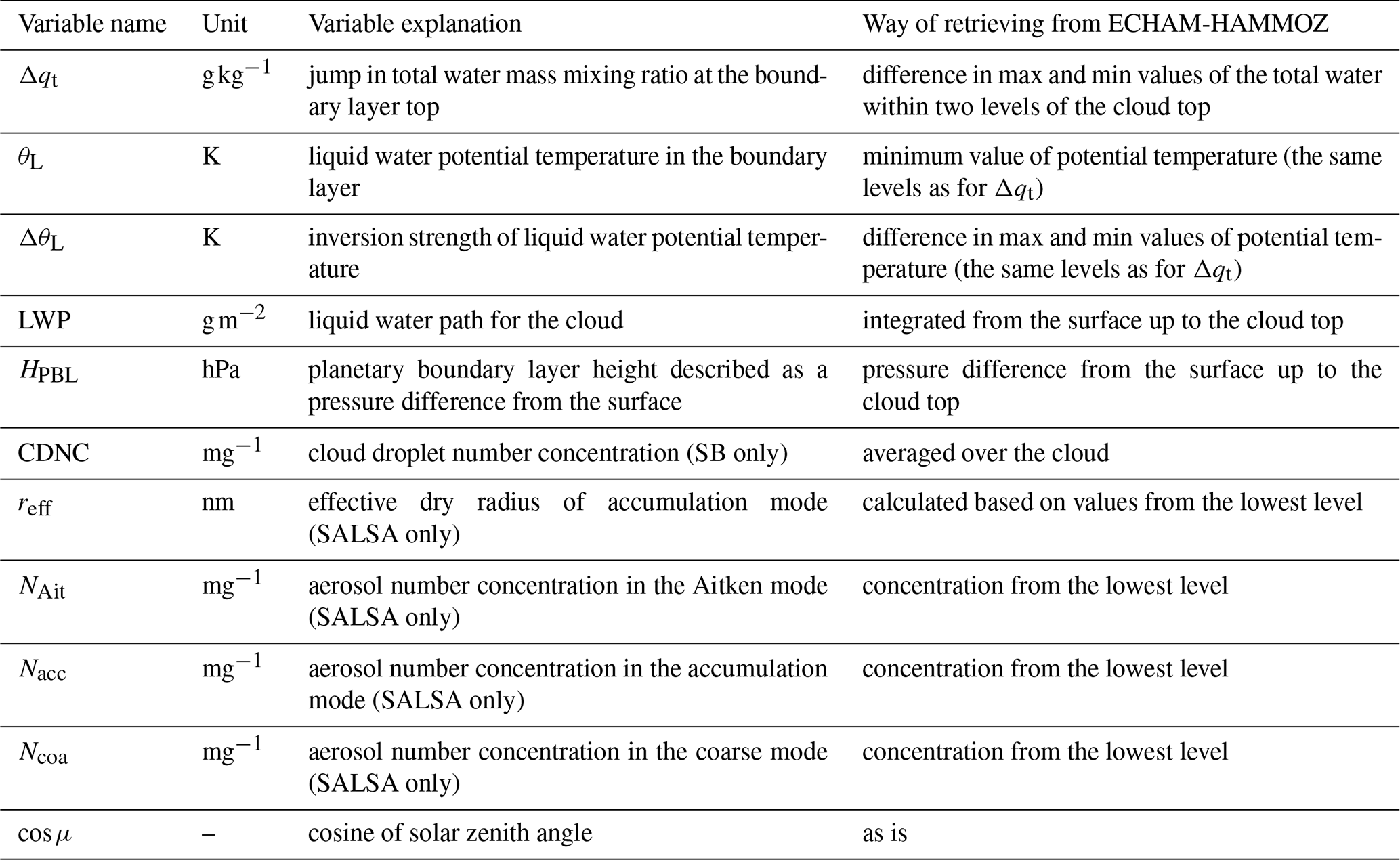
SB microphysics requires cloud droplet number concentration as input. On the other hand, SALSA needs aerosol size distributions and chemical composition or hygroscopicity. In order to reduce the number of variables, log-normal particle size modes are described by using effective dry radii (reff). The hygroscopicity parameter κ (Petters and Kreidenweis, 2007) in ECHAM-HAMMOZ depends on aerosol chemical composition, while the aerosol in SALSA is assumed to be sulfuric acid for which is constant. Sulfuric acid was chosen as the only chemical component of aerosols to limit computational expenses, and it resembles aged sea salt aerosols. When critical supersaturation for cloud activation is the same in ECHAM-HAMMOZ and SALSA, then , where r is the dry radius in ECHAM-HAMMOZ. The effective dry radius of the accumulation mode is considered a variable because this mode can be important for cloud activation. For Aitken and coarse modes we fixed the effective dry radii to 0.0105 and 0.4813 µm, respectively, based on their time averages in the source data. Aitken, accumulation and coarse modes have fixed standard deviations of 1.59, 1.59 and 2.0, respectively, in ECHAM-HAMMOZ, and these are used also in the LES runs.
2.2.2 Sampling the source data
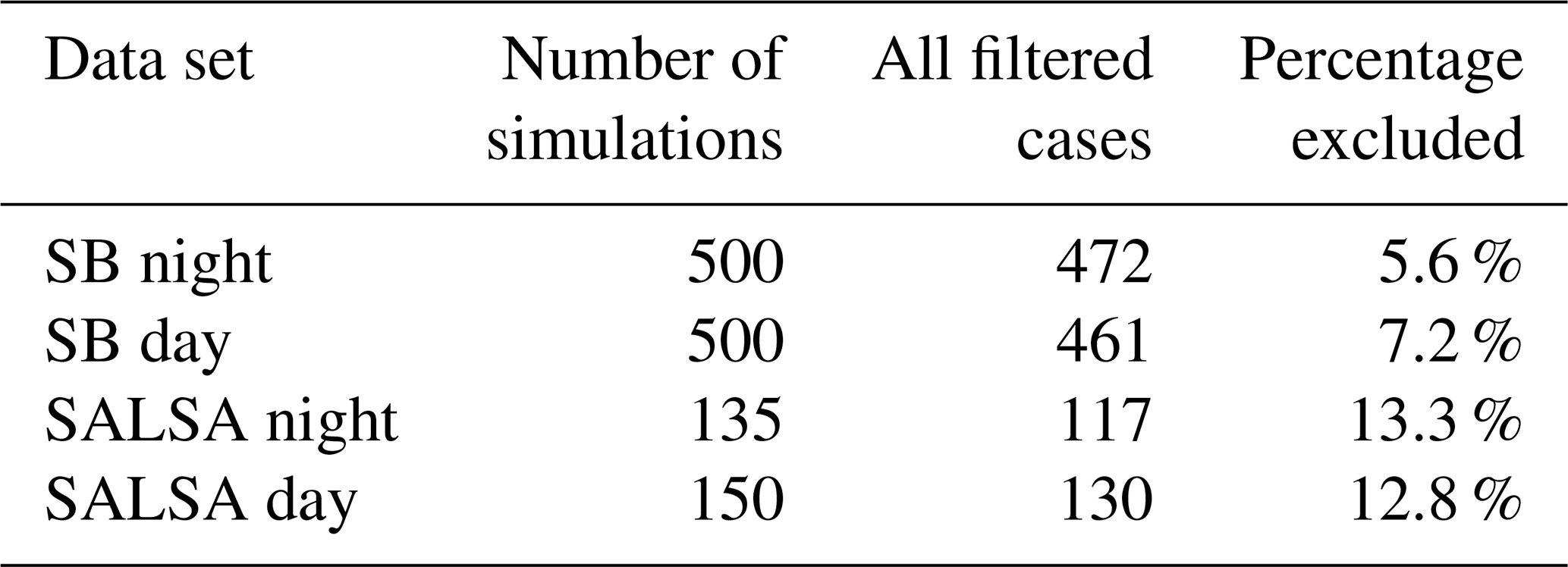
The next part of the pipeline is sampling representative subsets from the filtered source data (point 2 in Fig. 1). Here, these subsets are called designs (point C in Fig. 1). These are used to initialise the large-eddy simulations and further on as a part of inputs for the updraft parameterisations after filtering (Table 2).
Creating a design is a crucial part of the parameterisation development (Diggle and Lophaven, 2006). For instance, a Gaussian process emulator in general is accurate near the points it is trained with but loses accuracy as one tries to predict conditions far away from them (Rasmussen and Williams, 2006). Therefore, determining the distribution of the points (a good design) plays a vital role in the prediction. It is of key importance to identify regions where a higher accuracy is required, either due to their relevance to the application or simply because predictions are more often done there. On the other hand, one should not focus too heavily on any single region because of the diminishing return from each additional nearby point. As the designs are model-based, the aforementioned aspects imply two competing requirements of a design: (i) the design should cover the entire domain of interest, and (ii) it should focus on sub-regions of interest where a higher accuracy is desired (see also Liu and Vanhatalo, 2020).
In this work, we used a simple stratified sampling method based on binary space partitioning (BSP) trees (e.g. Fuchs et al., 1980; Tóth, 2005). The goal of the algorithm is to create a partitioning that represents the high-level distributional properties of the collection (Sect. 2.2.1) and then uniformly sample a point in each partition. By enforcing a single sample per partition, we ensure a space-covering property while still letting the distribution of the points in the collection guide on which areas to focus.
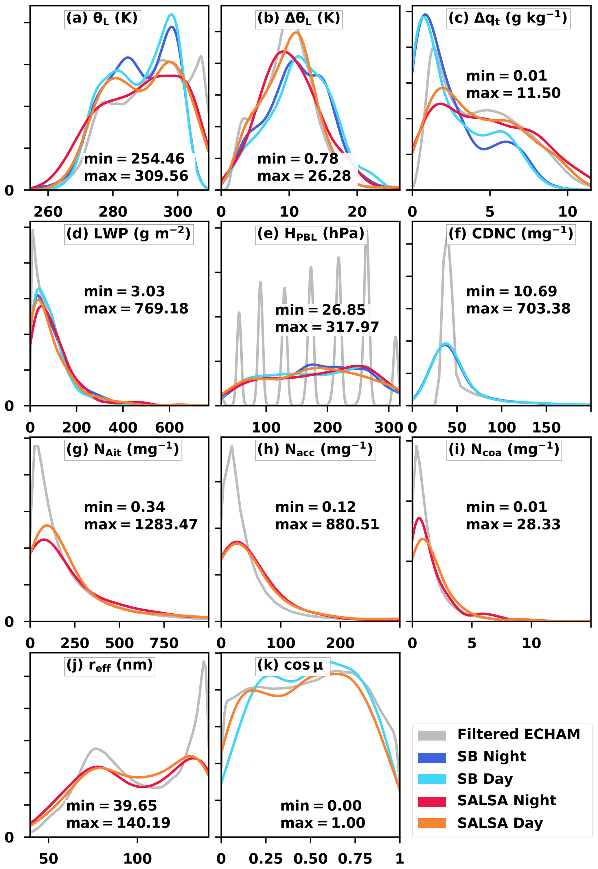
Figure 2Filtered ECHAM-HAMMOZ data and kernel-density-estimated (KDE) LES input variable probability density functions (PDFs). The highest values in panels (f–i) are not shown as the density is close to zero. Min and max values are extreme values of all LES sets (i.e. not ECHAM-HAMMOZ values).
The BSP method was used to generate separate day and night designs for both SB and SALSA microphysics. The designs are separate because they contain different variables. For example, the cosine of the solar zenith angle has an impact on updraft velocity only during the daytime. The number of samples taken from the source data for each design depends on the number of variables as well as the computational resources available for the LES runs. Both day and night SB designs have 500 samples, while SALSA designs have 135 and 150 samples in total for night and day, respectively. Ten samples per variable can be considered the minimum at least for the Gaussian process emulator (Loeppky et al., 2009).
The probability density function (PDF) of each design variable is given in Fig. 2. The numbers show the full range of values in the designs from min to max. The highest cloud droplet and mode number concentration values are excluded from the figures for clarity. The method used to calculate distributions for the design variables is the kernel density estimation (Scott, 1992), which smooths the PDF and was used due to the low number of samples. It should be noted that the spikes of HPBL values in filtered ECHAM-HAMMOZ data in Fig. 2e are related to the vertical discretisation of the model. We added noise to the HPBL values to obtain a smoother, i.e. more realistic, planetary boundary layer height distribution.
2.3 Setting up the LES runs
After creating the four designs (SB and SALSA microphysics, day and night), we generate the LES inputs and run the simulations (point 3 in Fig. 1). Initial temperature and humidity profiles for LES are reconstructed from the design variables (Table 1) while assuming a well-mixed cloud-topped marine boundary layer. With this assumption, the boundary layer total water mixing ratio (qt) was solved from the LWP, and boundary layer height was converted from the pressure difference to metres above sea surface.
Figure 3 shows an example of the initial temperature and humidity profiles that were generated using the five meteorological input variables. Here, inversion layer thickness is based on an assumed liquid water potential temperature gradient of 0.3 K m−1. Above the inversion layer, θL increases at a rate of 3 K km−1 and qt decreases linearly so that it would reach zero 2 km above the top of the inversion layer. Note that the hypothetical total water zero point would be at least 1 km above the top of the LES domain.
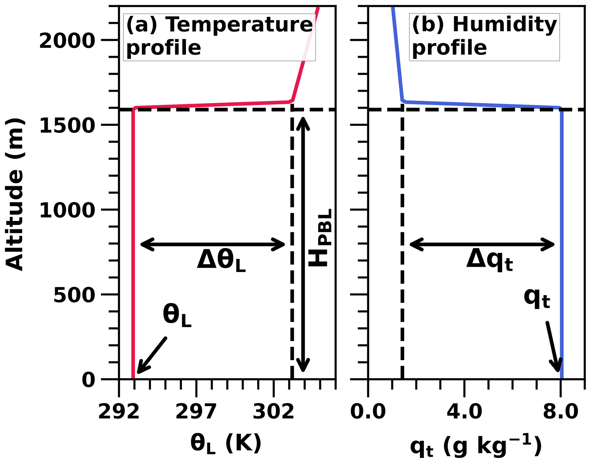
Figure 3An example of the initial atmospheric profiles generated from the meteorological input parameters.
The remaining design variables are related to cloud microphysics and solar radiation. Daytime simulations have a fixed solar zenith angle; i.e. it does not change with time. We did not include the diurnal cycle as that would disconnect the end state of the simulations from the input values, which would violate the underlying assumptions of the machine-learning-based approach presented in this study. For SB microphysics, the only cloud microphysical parameter is cloud droplet number concentration. The SALSA simulations are initialised with the specified tri-modal aerosol size distribution in each grid cell (Sect. 2.2.1).
The model also has options related to initialisation, surface interactions, radiative transfer, large-scale forcing and microphysics. For most of these, default values were used in the simulations, but the following parameters were adjusted. Initial horizontal wind profiles were set to 10 m s−1 in the east–west direction for all altitudes. Surface sensible and latent heat fluxes were set to zero, which is in line with the idealised initial temperature and humidity profiles. The radiative solver needs the surface skin temperature, which was set to be the same as the air temperature in the first model layer above the surface. Large-scale divergence was set to s−1.
In the simulations, horizontal grids cover 10 km in each direction with a 50 m resolution. The vertical grid is case-dependent so that it extends from the sea surface up to a height that is 1.333 times the planetary boundary layer height (HPBL). The vertical resolution is 10–20 m depending on the boundary layer height (maximum about 3000 m). The adaptive time step of the model was set to be 2 s minimum, and the statistics sampling time period was set to 300 s. Subgrid fluxes are calculated with the Smagorinsky model. The advection of momentum is based on fourth-order difference equations with the leapfrog method as a time-stepping scheme. The scalar advection uses a second-order flux-limited scheme. The time integration is executed with a simple forward Eulerian time-stepping method.
Coagulation, cloud-to-rain autoconversion and sedimentation processes were switched off during the first 1.5 h of spin-up, which allows enough time for turbulence to develop. The simulation time was limited to 3.5 h to prevent the model from drifting too far from the state representing the design variables. For the same reason, we nudged the liquid water potential temperature and SALSA aerosol concentrations towards their initial values using a relaxation time τ=3600 s. This choice for the relaxation parameter is a compromise value which aims to eliminate changes in boundary layer height that are too large while still allowing radiative cooling to create mixing. Aerosol was nudged only in the first grid layer above the sea surface.
Once the simulations were ready (point D in Fig. 1), we collected standard model output cloud top radiative cooling values and updraft velocities from the last simulation hour and calculated averages over the domain (point 4 in Fig. 1). These simulation statistics are used in creating the updraft parameterisations (point E in Fig. 1).
Although we show here only the few selected parameters, some additional details about the cloud evolution is provided in the Supplement. In the Supplement we show statistics about cloud development based on the difference between the initial and final states (Figs. S1–S3 in the Supplement). Figures S1 and S2 show that the cloud top and base heights do not change much during the simulations. However, the LWP decreases from the initial value (Fig. S3) because entrainment mixing at the cloud tops leads to sub-adiabatic liquid water mixing ratio profiles. In addition, precipitation removes some of the liquid water although precipitation rates are typically low (Fig. S4 in the Supplement). We also show that the tendencies of updraft velocities during the last simulation hour are close to zero (Fig. S5 in the Supplement), which indicates that the turbulence is fully developed. Finally, analysis of different decoupling measures (Figs. S6 and S7 in the Supplement) confirms that the majority of the simulations are not decoupled from the surface.
2.4 Updraft parameterisations
In this study we created three different updraft parameterisations (point 5 in Fig. 1). The first parameterisation is a simple linear fit (LF) based on cloud top radiative cooling (Zheng et al., 2016) (Sect. 2.4.1); the second is the same linear fit with a random forest (LFRF) improvement (Sect. 2.4.2); and the third is a Gaussian process emulator (GPE) (Sect. 2.4.3). Parameterisations are trained based on LES run outputs, where parameterisation input values can include design variables (i.e. LES run input variables, Table 1) and/or LES run outputs (i.e. cloud radiative cooling). The objective of the parameterisations is to reproduce the simulated domain mean positive updraft velocities at the cloud base (LES output) and predict those according to selected input variables. Since training input values include both LES inputs and outputs, it is vital that the simulations do not drift too far away from the initial state.
We used only one non-machine learning method (LF; Zheng et al., 2016) as it has only one input variable and hence is possibly the simplest parameterisation available. Yet, as we will show below, it still performs quite well. Here, we focus on introducing machine-learning-based parameterisations for which the LF parameterisation serves as a baseline.
The main statistical measures for parameterisation intercomparisons are the coefficient of determination (R2) and root mean square error (RMSE). R2 is a measure that tells us how well the regression model fits the data. R2 equals the proportion of variance in the dependent variable (y-axis values) that can be explained by the independent variable (x-axis value). However, R2 does not indicate whether there are enough data points to make a solid conclusion. RMSE is frequently used to measure the differences between predicted values (here parameterisations) and the values regarded as a ground truth (LES runs). RMSE is dependent on the scale of the numbers used, i.e. has the same physical unit as in the original data, and is sensitive to outliers.
2.4.1 Linear fit (LF)
The linear fit approach is inspired by the observational study of Zheng et al. (2016), who found a strong correlation between cloud top radiative cooling (CTRC) and updraft velocity at the cloud base (Wb). Based on that, they proposed a parameterisation as follows:
where Wb and CTRC have units of cm s−1 and W m−2, respectively. Here, negative CTRC values indicate cooling. This parameterisation is based on both day and night radar observations and radiative transfer model simulations on non-precipitating marine stratocumulus clouds.
Here, we make a linear fit, Wb, as a function of CTRC, where data are obtained from the LES runs, and compare it with the parameterisation of Zheng et al. (2016). We did not exclude precipitating cases because this would have limited the applicability of the method in a global model. The parameterisation coefficients were derived separately for the SB and SALSA microphysics and for day and night.
2.4.2 Linear fit improved with random forest (LFRF)
The second parameterisation builds on the linear updraft velocity model (Sect. 2.4.1). However, instead of directly predicting the updraft velocity, this parameterisation predicts the approximation error, i.e. the difference between the LF and the LES output for given design variable values (Sect. 2.3). This error prediction is then used to correct the predictions of the linear fit. The approach used in this study is similar to the approximation error correction method introduced in Lipponen et al. (2013, 2018). In Lipponen et al. (2018), it was shown that predicting and correcting the approximation error of the output of an approximative model often lead to more accurate results than directly predicting the model output.
In this study, we trained a random forest (Breiman, 2001) regression model to correct for the approximation error in the linear updraft velocity model. A random forest regressor consists of an ensemble of binary regression trees. Random forests can learn non-linear functions, and they are relatively tolerant to overfitting. As a result, random forests have provided highly accurate results in many applications. For more information on random forests and on training and evaluation of the models, see Breiman (2001). In this study, the random forest regressor model was trained using the scikit-learn machine learning package (Pedregosa et al., 2011). The random forest model consisted of 200 regression trees; otherwise, the default training parameters of the scikit-learn package were used. Inputs of the approximation error correction model during training include the design variables and cloud top radiative cooling from the LESs. The software used to produce the results is available on GitHub (Ahola et al., 2022b).
2.4.3 Gaussian process emulator (GPE)
The third method we used is a Gaussian process emulator (O'Hagan, 1978, 2006) to directly predict the updraft velocity as a function of design variables (Table 1). Our implementation is based on the Gaussian process regressor given in the scikit-learn machine learning package (Pedregosa et al., 2011) that uses Rasmussen and Williams (2006) as the theoretical foundation. Gaussian process regression models are based on multivariate normal distributions and covariance functions. Given an input data point, a Gaussian process regression model trained with a training data set can predict the probability distribution of the outputs corresponding to the input data. For more information on training and evaluation of the Gaussian process regression models, see, for example, Rasmussen and Williams (2006). The software used to produce the results is available on GitHub (Ahola et al., 2021a, 2022b).
2.5 Post-processing the LES runs
In this study we focus on the updraft velocity at the cloud base where the majority of the cloud droplets form. From the different definitions of cloud base updraft velocity (Romakkaniemi et al., 2009), we found that the following gives the best agreement with the Zheng et al. (2016) observations:
where Wi is positive updraft velocity at the lowest cloudy grid cell (liquid water content LWC>0.01 g kg−1) in a column and c is the number of cloudy columns. Negative Wi values (downdrafts) are set to zero, i.e. ignored. The sum includes 3D LES model outputs from the last simulation hour.
The linear fit (LF) and linear fit improved with random forest (LFRF) are based on cloud top radiative cooling (CTRC), which is calculated from the LES outputs as
where Ri,base and Ri,top are the net (short-wave + long-wave) radiative fluxes at the cloud base and top, respectively. Because net fluxes are defined to be upwardly positive, negative CTRC means cooling. The sum includes 3D (SB microphysics) or horizontally averaged 1D (SALSA microphysics) model outputs that are averaged over the last simulation hour. For SALSA microphysics, 3D radiation fields were not saved in order to reduce the high number of outputs. In the SB simulations, differences between CTRC values calculated from the 3D and 1D radiation outputs were found to be negligible.
Training data for the parameterisations include the design variables and the corresponding LES updraft velocity (Eq. 2) and CTRC (Eq. 3) outputs. Some simulations that diverged significantly from the initial conditions produced outliers, which reduced the accuracy of the parameterisations in representing the rest of the cases. Therefore, in all following results, before creating a parameterisation, we filtered out simulations where the cloud fraction was smaller than 0.61 or the cloud top rose more than 10 % (see Table 2). In an initial analysis conducted when calculating the LF, these cases were found to produce most of the outliers. All filtering parameter values were the last retrievable values from the simulations. The cases where the cloud top rose more than 10 % were mostly related to weak temperature inversions at the cloud top (Sect. 2.2.1). For example, our temperature inversions start from 0.78 K (Fig. 2b), while Feingold et al. (2016) excluded values lower than 6 K. Weak temperature inversions are less effective in reducing entrainment mixing, which causes the deepening of the boundary layer (Wood, 2012). Nudging the model fields towards the initial conditions was used to suppress the issue, but it was not entirely eliminated. Using more restrictive initial conditions would have produced a more idealised stratocumulus sample, but at the same time we would have lost the ability to predict updraft velocities for less ideal cases commonly present in ECHAM-HAMMOZ simulation. In short, the limits for the filter (Table 2) were chosen so that they eliminate clear outliers from the linear fit. Changing these thresholds would have an impact for the accuracy of the linear fit parameterisation simply by changing the number of outliers but not so for the two machine learning parameterisations that can represent complex dependencies. In other words, the LF is sensitive to the thresholds, while the two machine learning methods are less sensitive.
3.1 Parameterisation intercomparison
In the comparisons of the three parameterisations, LES runs are regarded as the ground truth, the LF is regarded as a baseline simple parameterisation, the LFRF improves the LF with a machine learning method and the GPE is a stand-alone machine learning method. The presented parameterisations are compared to each other and the LES runs.
The linear fit (LF) to simulated updraft and CTRC values overlaps quite well with the parameterisation from the Zheng et al. (2016) study (marked with a grey line and shading) especially in daytime simulations (Fig. 4). In nighttime simulations, the cloud radiative cooling explains much less of the variance of updraft velocity than during the daytime, and the linear fit nighttime R2 values for SB and SALSA are 0.36 (Fig. 4a) and 0.29 (Fig. 4c), respectively, compared to 0.67 (Fig. 4b) and 0.56 (Fig. 4d) during the daytime. The daytime simulations make a better fit because they have a wider distribution of radiative cooling values due to the large variability in solar radiation. In the absence of solar radiation, CTRC values in SB microphysics nighttime simulations are clustered around the value of −70 W m−2 and the exceptions are related to high boundary layer heights (increased CTRC and Wb), thin clouds (reduced CTRC and Wb) and rising clouds (reduced Wb). A cooling value of −70 W m−2 is a typical difference in net long-wave radiation between the cloud top and cloud base for shallow boundary layer clouds.
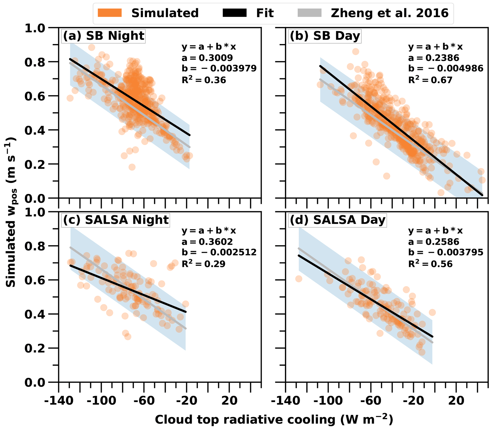
Figure 4Simulated updraft velocities as a function of simulated cloud top radiative cooling values. Also shown are the linear fits to the data. R2 is the coefficient of determination. SB and SALSA refer to Seifert–Beheng bulk microphysics and sectional microphysics, respectively. In daytime simulations, the solar zenith angle was used as one of the input parameters for the simulations. The grey lines and shading represent the Zheng et al. (2016) parameterisation with its uncertainty range.
Figure 5 shows the evaluation of the three different parameterisations, linear fit (LF), linear fit improved with random forest (LFRF) and Gaussian process emulator (GPE), based on a cross-validation approach. To obtain the predicted points, training data are shuffled randomly and then a 10-fold cross-validation is used. This means that for each fold, 90 % of the training data are used to train the parameterisation and predicted values are retrieved for the remaining 10 % of the points. When comparing parameterisations and simulation sets, R2 and RMSE values are in line with each other, meaning that as R2 increases (i.e. better fit), RMSE decreases (i.e. smaller error).
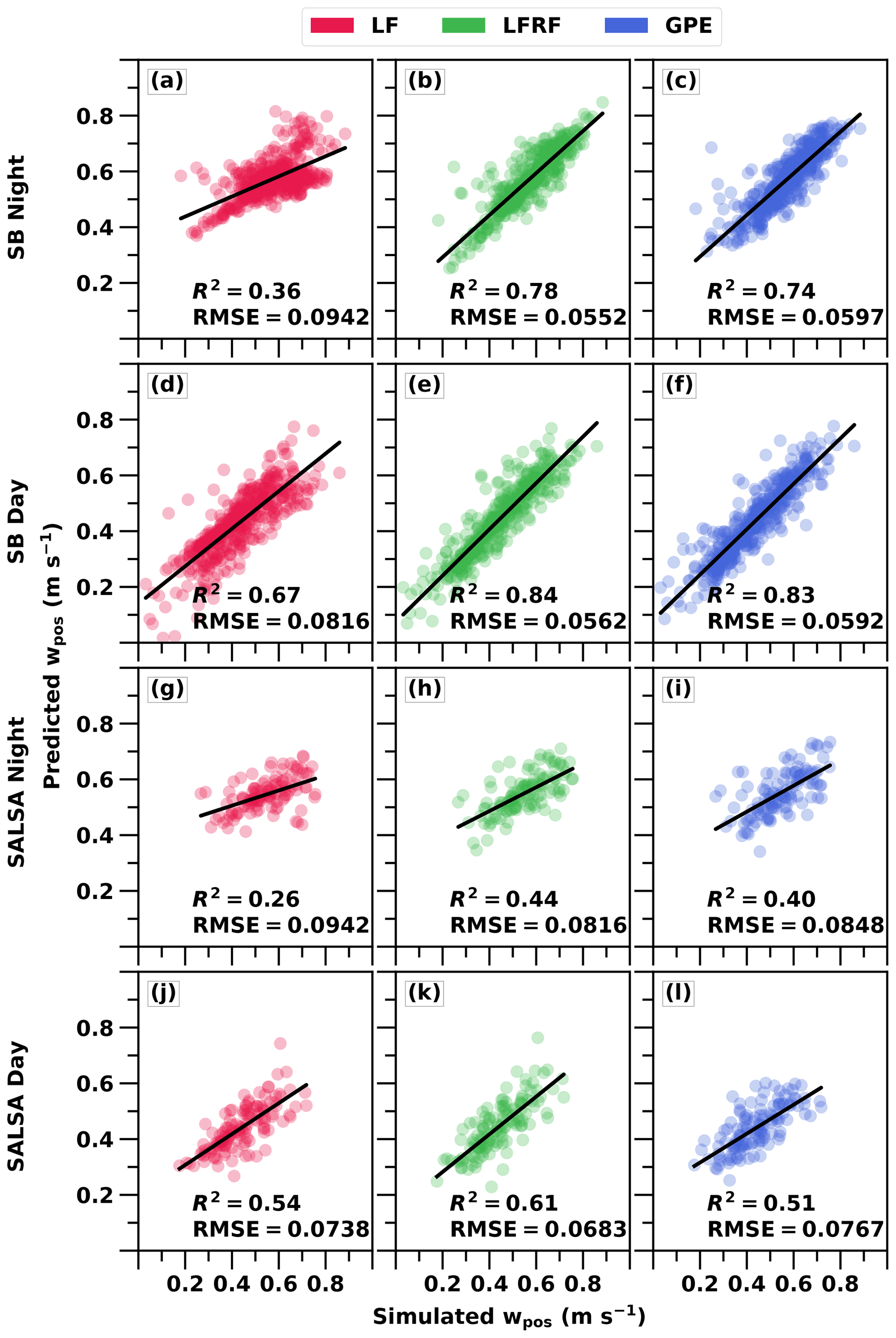
Figure 5Predicted updraft velocities from different parameterisations vs. simulated updraft velocities. (a, d, g, j) Linear fit (LF); (b, e, h, k) linear fit improved with random forest (LFRF); (c, f, i, l) Gaussian process emulator (GPE). Coefficient of determination (R2) and root mean square error (RMSE, units of m s−1) values are also given.
Figure 5 shows that the LFRF performs better than the other methods in all simulation sets based on R2 and RMSE values. The GPE is a close second in all but the daytime SALSA simulations. Both the LFRF and the GPE work generally well. The probable reason why the LFRF method performs so well, outperforming even the GPE, is that it is supported with an embedded dependency, the linear model LF. This is in line with Lipponen et al. (2013, 2018), who showed that including a dependency (i.e. correcting a rough empirical model with random forest) improved results compared to a pure random forest learning method. The LF is the least accurate method in all simulation sets, except in the SALSA day set where it outperforms the GPE only slightly. Because the LF shows worse results during the night than during the day (see Fig. 4), there is more room for improvement for the machine learning methods during the nighttime.
Parameterisations perform slightly better for simulation sets with SB than sets with SALSA microphysics. One reason for this is that accounting for aerosol–cloud interactions increases the variability in model predictions as prognostic supersaturation schemes increase degrees of freedom. Hence, the variability can be difficult to capture in a parameterisation based on a relatively small set of training data. This additional variability can be seen as lower R2 values in Fig. 4. The other main reason is that the number of computationally heavy SALSA simulations had to be limited to the lowest number possible. A limited learning data set will have an impact on the accuracy of the predictions.
3.2 Permutation feature importance
We calculated permutation feature importance to reveal the significance of individual input parameters for the LFRF and GPE updraft velocity parameterisations. The permutation feature importance is defined to be the decrease in a model score (R2) when a single feature (input variable) value is randomly shuffled (Breiman, 2001; Pedregosa et al., 2011). This method breaks the relationship between the feature and the target; thus the decrease in the model score shows how much the model depends on the feature. This technique does not depend on the model used, and it can be applied many times with different permutations of the feature. A high feature importance value means that the variable is important for the model. Some variables had small negative feature importance values, meaning that the variable actually decreased the model score. These values were set to zero as small negative values can be regarded as numerical artefacts. The legend of Fig. 6 shows the overall order of significance based on the mean of fractional (absolute values divided by the total in each panel of Fig. 6) feature importances.
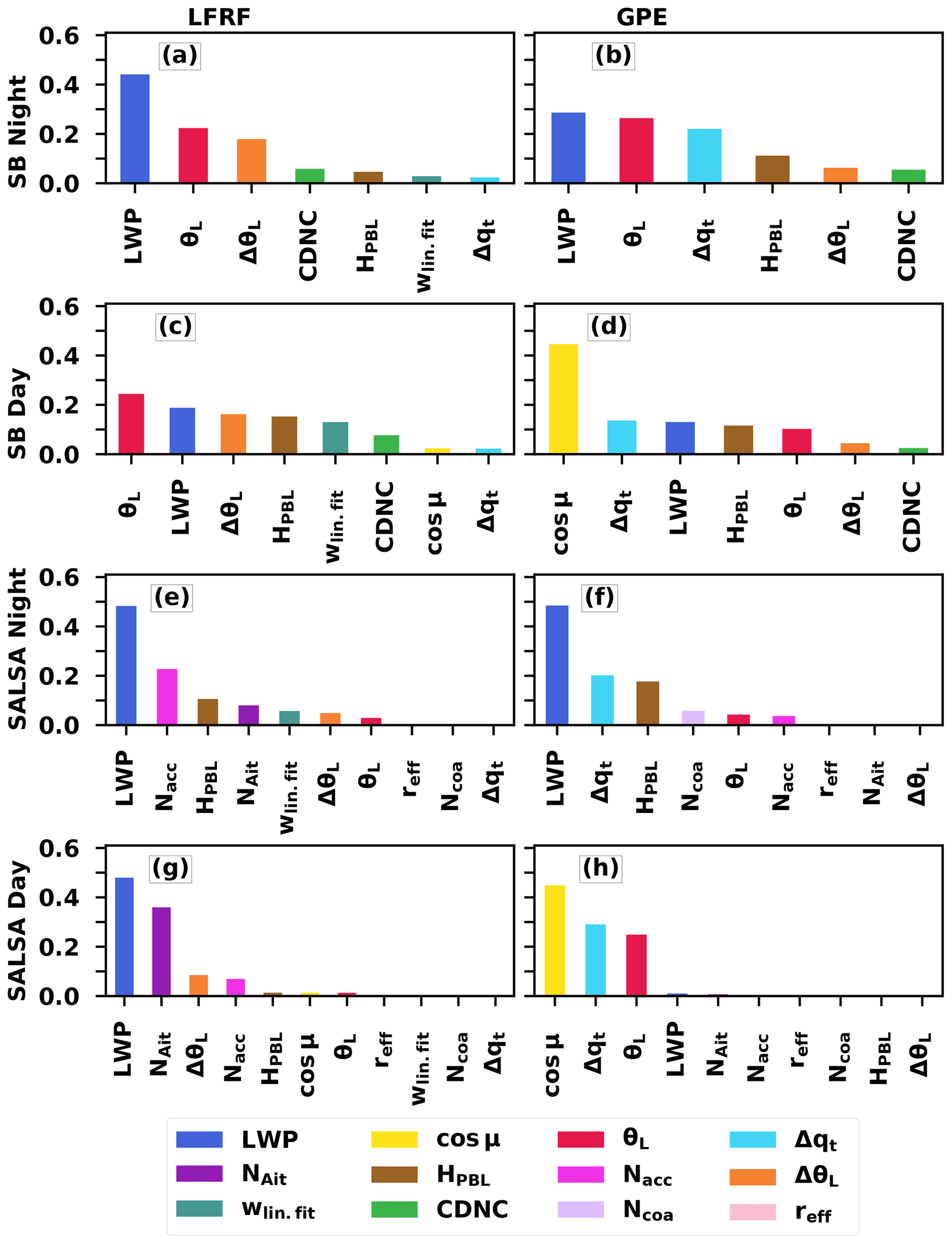
Figure 6Permutation feature importance of (a, c, e, g) the linear fit improved with random forest (LFRF) and (b, d, f, h) the Gaussian process emulator (GPE).
It should be noted that, as the GPE is a stand-alone method, those variables that physically contribute to updraft velocity are also the most important features in Fig. 6. On the other hand, when improving the LF with the learning method (LFRF), an important physical aspect (CTRC) is already incorporated, and variables that contribute to the error of the LF are shown as important features. Hence, the GPE is easier to interpret physically, while the results for the LFRF tell us which variables, beyond radiative cooling, impact the updraft velocity in the selected set-up. The LFRF can also be considered a piecewise-defined constant function: when within a certain subset of inputs, some features can be more important than when outside the subset. As the learning method with the LFRF is random, it enables these kinds of subsets to be very small and sharp-edged, meaning that training points outside a specific subset do not affect the outputs of the subset. In contrast, the GPE makes predictions based on the whole training point domain. These distinct characteristics of the GPE and LFRF indicate that important features for the GPE are probably relevant in the whole training domain, while for the LFRF, the features may be important only in certain subdomains.
Figure 6 shows that the most important parameters are the LWP, cos μ, θL, Δqt and NAit. Of these variables, NAit is a microphysical variable and specific only to the SALSA microphysics scheme. LWP, θL and Δqt are meteorological variables and common to all simulation sets. cos μ is used only in the daytime simulation sets.
Unravelling the meaning of these variables, it is simplest to start with cos μ as it affects updraft velocity quite straightforwardly. For the GPE parameterisation during the daytime, cos μ is the most important feature because it strongly influences cloud top radiative cooling, which indicates that the learning method grasps significant physical aspects that affect updraft velocity. For the LFRF, cos μ is not that significant since the linear fit for the updraft velocity (wlin.fit) already incorporates solar radiation dependency through cloud top radiative cooling.
The LWP is important for both the LFRF and the GPE. First, radiative cooling requires a sufficient LWP, so it is important for the GPE. On the other hand, a high LWP increases precipitation probability. Precipitation causes deviations from the linear trend of Wb vs. CTRC by stabilising the boundary layer and reducing updraft velocities, so the LWP is important for the LFRF as well. Zheng et al. (2016) used a radar to measure vertical velocities, so they had to exclude precipitating cases. Our parameterisations are aimed at GCMs where precipitation cannot be excluded as updraft velocity at the cloud base is solved before calculating the cloud droplet number concentration and precipitation formation.
Boundary layer liquid water potential temperature (θL) and boundary layer height (HPBL) determine the cloud top temperature, so they have a direct impact on radiative cooling rates. This can be seen with the GPE. With the LFRF radiative cooling is already incorporated with wlin.fit, but the LF does not work well with high and low θL values; hence θL is an important feature with the LFRF.
A strong humidity jump (Δqt) means a dry free troposphere, which allows strong radiative cooling. Radiative cooling is an important factor for turbulence, and therefore, Δqt is an important feature for the GPE. The LF accounts for the radiative cooling, so Δqt is not an important feature with the LFRF.
Regarding aerosol parameters, CDNC is not shown as an important feature with GPE and SB microphysics. This is likely because the bulk model uses saturation adjustment to calculate cloud water mixing ratios. However, with SALSA, the droplet concentration change affects the condensation–evaporation rate and buoyancy and thus updrafts, which consequently is seen as high importances with aerosol parameters. This phenomenon (i.e. high aerosol-related feature importances) is better shown with the LFRF (Fig. 6e and g) as this is most likely a significant characteristic only within a subset of simulations with a low aerosol concentration and the GPE does not pick it up that well as it is not a common feature. Interestingly with the LFRF, the relative role of θL seems to be smaller when SALSA is employed instead of SB.
In this study we present three cloud base updraft velocity parameterisations which are based on detailed cloud simulations that can be used in global atmospheric models. The parameterisations represent the predictions of the large-eddy simulation model UCLALES-SALSA (Tonttila et al., 2017) for a wide range of marine boundary layer clouds described by the global climate model ECHAM-HAMMOZ. One parameterisation is a linear fit (LF) depending on cloud top radiative cooling only. The LF was first presented in Zheng et al. (2016) and is based on cloud observations. Another is based on the linear fit which is improved with a random forest model (LFRF). The random forest model was trained to predict the error of the linear fit as a function of parameters describing marine boundary layer clouds. The third is a stand-alone Gaussian process emulator (GPE) for predicting updraft velocities based on the cloud parameters.
As can be expected, the simple LF works well for cases where radiative cooling is the main driver of turbulence. The other machine learning techniques perform better because they account for additional variables such as cloud thickness and inversion strength, which have an additional influence on turbulence via processes like cloud top entrainment mixing and evaporative cooling and drizzle formation (Wood, 2012). Overall, the LFRF performs slightly better than the GPE.
When choosing between the LFRF and GPE, there are some points that should be considered. The GPE is purely based on machine learning without any underlying information about physical processes, while the LFRF includes the effect of cloud top radiative cooling. Therefore, when extrapolating outside of the range of the training inputs, the GPE prediction is the mean of the training outputs that may not be a good prediction. The LFRF, on the other hand, is reduced to the radiative cooling described by the linear fit when outside of the range of training outputs. The downside of the LFRF method is that it requires the value for the cloud top radiative cooling (CTRC) from the host model, which must be taken from the previous model time step. As a result, any uncertainties in the input CTRC will influence the predictions, while CTRC is not needed for the GPE. On the other hand, using CTRC as an input provides a possibility of also extending the LFRF to cases with thin overlying cloud layers, whereas extending the GPE to such cases would require including these cases in the training set.
We developed updraft parameterisations for two different cloud microphysics modules implemented in UCLALES-SALSA. One microphysics module (SALSA) accounts for aerosol–cloud interactions, and the other (SB) uses prescribed values for CDNC. Full prediction of the effect of aerosols on clouds and updraft velocity is complicated by the fact that meteorological parameters such as the inversion strength and the liquid water path dominate over aerosol effects. The increased computational cost of SALSA also limited the size of the training data set, which reduced the accuracy of the predictions. Nevertheless, we were able to show that aerosol number concentration has an impact on updraft velocities. In addition, SALSA could be used to predict properties that are more dependent on aerosol such as rain formation.
To conclude, machine learning techniques are becoming commonly used methods for parameterising complex dependencies (e.g. Rasp et al., 2018). Our work shows that the dependency of updraft velocity on the boundary layer state can be predicted with a reasonable accuracy and machine learning methods are able to also capture the effect of variables that are important only in a limited subset of all possible conditions, as is the case with aerosol number concentrations. Our results also show that machine learning is effective when it is supported with an underlying physical dependency, which is in line with previous studies (Lipponen et al., 2013, 2018; Silva et al., 2021; Kashinath et al., 2021). The parameterisations introduced are valid only for marine stratocumulus, but extension of the training set to cover the effects of surface heat fluxes and wind shear would improve the physical foundation of updraft parameterisations and increase the applicability of the method to continental stratiform boundary layer clouds also (e.g. Matheou and Teixeira, 2019).
Filter source data (ECHAM-HAMMOZ) are available at https://doi.org/10.5281/zenodo.5343428 (Nordling, 2021). The BSP algorithm is available at https://doi.org/10.5281/zenodo.5343366 (Alper and Liu, 2021). Designs are available at Zenodo: SB microphysics during the nighttime (Alper, 2021d), SB microphysics during the daytime (Alper, 2021c), SALSA microphysics during the nighttime (Alper, 2021b) and SALSA microphysics during the daytime (Alper, 2021a). For creating inputs for training simulations based on the design, see https://doi.org/10.5281/zenodo.5346765 (Ahola and Raatikainen, 2021). For LES runs with UCLALES-SALSA, ECLAIR branch, see https://doi.org/10.5281/zenodo.5346768 (Tonttila et al., 2021b). Post-processing training simulations are available at https://doi.org/10.5281/zenodo.5346789 (Tonttila et al., 2021a). Configuration files for result and figure scripts are available at https://doi.org/10.5281/zenodo.5346794 (Ahola, 2021). For creating parameterisations, see https://doi.org/10.5281/zenodo.5336989 (Ahola et al., 2022b). The Gaussian process emulator script is available at https://doi.org/10.5281/zenodo.5383581 (Ahola et al., 2021a). The library for Python scripts is available at https://doi.org/10.5281/zenodo.6075748 (Ahola, 2022a). For plotting the results, see https://doi.org/10.5281/zenodo.6075779 (Ahola, 2022b). Data of LES runs are available at https://doi.org/10.23728/FMIB2SHARE.179721B8 F65643718FF4A5FECF230F7C (Ahola et al., 2022a). Results are available at https://doi.org/10.23728/FMIB2SHARE.477AF 35BE02F4A158E2F7E852022EC60 (Ahola et al., 2021b).
The supplement related to this article is available online at: https://doi.org/10.5194/acp-22-4523-2022-supplement.
KN provided the ECHAM-HAMMOZ data with help from HarK, AIP and PR. The design of LES runs was made by MEA. JA, TR, JT, HarK and SR contributed in developing the UCLALES-SALSA model, and JA ran the simulations. JA created the LF results with help from TR. JA created the LFRF results with development help from AL and AK. JA created the GPE results with development help from MEA, AK, JL, JPK and AL. JA plotted and analysed the data with help from TR, SR and AL. JA wrote the paper with TR and SR with comments from all co-authors. TR, HarK, AIP, SR, PR and HanK provided senior scientific guidance for the project. HanK came up with the emulation concept and supervised the project.
The contact author has declared that neither they nor their co-authors have any competing interests.
Publisher's note: Copernicus Publications remains neutral with regard to jurisdictional claims in published maps and institutional affiliations.
The authors wish to acknowledge CSC – IT Center for Science, Finland, for computational resources.
This research has been supported by the H2020 European Research Council (ECLAIR (grant no. 646857) and FORCeS (grant no. 821205)) and the Academy of Finland (grant nos. 322532 and 309127).
This paper was edited by Barbara Ervens and reviewed by two anonymous referees.
Ahola, J.: LES-emulator-04configFiles: v1.0.1, Zenodo [code], https://doi.org/10.5281/zenodo.5383581, 2021. a
Ahola, J.: LES-03plotting: v2.0.1, Zenodo [code], https://doi.org/10.5281/zenodo.6075748, 2022a. a
Ahola, J.: LES-emulator-03plotting: v1.1, Zenodo [code], https://doi.org/10.5281/zenodo.6075779, 2022b. a
Ahola, J. and Raatikainen, T.: LES-emulator-01prepros: v1.0, Zenodo [code], https://doi.org/10.5281/zenodo.5336989, 2021. a
Ahola, J., Korhonen, H., Tonttila, J., Romakkaniemi, S., Kokkola, H., and Raatikainen, T.: Modelling mixed-phase clouds with the large-eddy model UCLALES–SALSA, Atmos. Chem. Phys., 20, 11639–11654, https://doi.org/10.5194/acp-20-11639-2020, 2020. a
Ahola, J., Kukkurainen, A., Alper, M. E., Liu, J., and Lipponen, A.: GPEmulatorPython: v1.0, Zenodo [code], https://doi.org/10.5281/zenodo.5347718, 2021a. a, b
Ahola, J., Raatikainen, T., Alper, M. E., Keskinen, J.-P., Kokkola, H., Kukkurainen, A., Lipponen, A., Liu, J., Nordling, K., Partanen, A.-I., Romakkaniemi, S., Räisänen, P., Tonttila, J., and Korhonen, H.: Updraft velocity parameterisation data and figures of “Parameterising cloud base updraft velocity of marine stratocumuli” -manuscript, B2Share [data set], https://doi.org/10.23728/FMI-B2SHARE.477AF35BE02F4A158E2F7E852022EC60, 2021b. a
Ahola, J., Raatikainen, T., Alper, M. E., Keskinen, J.-P., Kokkola, H., Nordling, K., Partanen, A.-I., Romakkaniemi, S., Räisänen, P., Tonttila, J., and Korhonen, H.: LES simulations of “Parameterising cloud base updraft velocity of marine stratocumuli” -manuscript, B2Share [data set], https://doi.org/10.23728/FMI-B2SHARE.179721B8F65643718FF4A5FECF230F7C, 2022a. a
Ahola, J., Raatikainen, T., Kukkurainen, A., Alper, M. E., Liu, J., Keskinen, J.-P., and Lipponen, A.: LES-emulator-02postpros: v2.1, Zenodo, https://doi.org/10.5281/zenodo.6075756 [code], 2022b. a, b, c
Alper, M. E.: DESIGN: SALSA daytime 150 simulations, Zenodo [data set], https://doi.org/10.5281/zenodo.5346794, 2021a. a
Alper, M. E.: DESIGN: SALSA nighttime 135 simulations, Zenodo [data set], https://doi.org/10.5281/zenodo.5346789, 2021b. a
Alper, M. E.: DESIGN: SB 500 daytime simulations, Zenodo [data set], https://doi.org/10.5281/zenodo.5346768, 2021c. a
Alper, M. E.: DESIGN: SB 500 nighttime simulations, Zenodo [data set], https://doi.org/10.5281/zenodo.5346765, 2021d. a
Alper, M. E. and Liu, J.: ECLAIRscripts/StateSpaceDesign, Zenodo [code], https://doi.org/10.5281/zenodo.5343366, 2021. a
Bennartz, R.: Global assessment of marine boundary layer cloud droplet number concentration from satellite, J. Geophys. Res.-Atmos., 112, D02201, https://doi.org/10.1029/2006JD007547, 2007. a
Bougiatioti, A., Nenes, A., Lin, J. J., Brock, C. A., de Gouw, J. A., Liao, J., Middlebrook, A. M., and Welti, A.: Drivers of cloud droplet number variability in the summertime in the southeastern United States, Atmos. Chem. Phys., 20, 12163–12176, https://doi.org/10.5194/acp-20-12163-2020, 2020. a
Breiman, L.: Random Forests, Mach. Learn., 45, 5–32, https://doi.org/10.1023/A:1010933404324, 2001. a, b, c
Diggle, P. and Lophaven, S.: Bayesian Geostatistical Design, Scand. J. Stat., 33, 53–64, https://doi.org/10.1111/j.1467-9469.2005.00469.x, 2006. a
Feingold, G., McComiskey, A., Yamaguchi, T., Johnson, J. S., Carslaw, K. S., and Schmidt, K. S.: New approaches to quantifying aerosol influence on the cloud radiative effect, P. Natl. Acad. Sci. USA, 113, 5812–5819, https://doi.org/10.1073/pnas.1514035112, 2016. a
Fu, Q. and Liou, K. N.: Parameterization of the Radiative Properties of Cirrus Clouds, J. Atmos. Sci., 50, 2008–2025, https://doi.org/10.1175/1520-0469(1993)050<2008:POTRPO>2.0.CO;2, 1993. a
Fuchs, H., Kedem, Z. M., and Naylor, B. F.: On Visible Surface Generation by a Priori Tree Structures, in: Proceedings of the 7th Annual Conference on Computer Graphics and Interactive Techniques, vol. 14 of SIGGRAPH '80, Association for Computing Machinery, New York, NY, USA, 1 July 1980, 124–133, https://doi.org/10.1145/965105.807481, 1980. a
Golaz, J.-C., Salzmann, M., Donner, L. J., Horowitz, L. W., Ming, Y., and Zhao, M.: Sensitivity of the Aerosol Indirect Effect to Subgrid Variability in the Cloud Parameterization of the GFDL Atmosphere General Circulation Model AM3, J. Climate, 24, 3145–3160, https://doi.org/10.1175/2010JCLI3945.1, 2011. a
Honnert, R., Efstathiou, G. A., Beare, R. J., Ito, J., Lock, A., Neggers, R., Plant, R. S., Shin, H. H., Tomassini, L., and Zhou, B.: The Atmospheric Boundary Layer and the “Gray Zone” of Turbulence: A Critical Review, J. Geophys. Res.-Atmos., 125, e2019JD030317, https://doi.org/10.1029/2019JD030317, 2020. a
Kacarab, M., Thornhill, K. L., Dobracki, A., Howell, S. G., O'Brien, J. R., Freitag, S., Poellot, M. R., Wood, R., Zuidema, P., Redemann, J., and Nenes, A.: Biomass burning aerosol as a modulator of the droplet number in the southeast Atlantic region, Atmos. Chem. Phys., 20, 3029–3040, https://doi.org/10.5194/acp-20-3029-2020, 2020. a
Kashinath, K., Mustafa, M., Albert, A., Wu, J.-L., Jiang, C., Esmaeilzadeh, S., Azizzadenesheli, K., Wang, R., Chattopadhyay, A., Singh, A., Manepalli, A., Chirila, D., Yu, R., Walters, R., White, B., Xiao, H., Tchelepi, H. A., Marcus, P., Anandkumar, A., Hassanzadeh, P., and Prabhat: Physics-informed machine learning: case studies for weather and climate modelling, Philos. T. Roy. Soc. A, 379, 20200093, https://doi.org/10.1098/rsta.2020.0093, 2021. a, b
Khairoutdinov, M., Randall, D., and DeMott, C.: Simulations of the Atmospheric General Circulation Using a Cloud-Resolving Model as a Superparameterization of Physical Processes, J. Atmos. Sci., 62, 2136–2154, https://doi.org/10.1175/JAS3453.1, 2005. a
Khairoutdinov, M. F. and Randall, D. A.: A cloud resolving model as a cloud parameterization in the NCAR Community Climate System Model: Preliminary results, Geophys. Res. Lett., 28, 3617–3620, https://doi.org/10.1029/2001GL013552, 2001. a
Kokkola, H., Korhonen, H., Lehtinen, K. E. J., Makkonen, R., Asmi, A., Järvenoja, S., Anttila, T., Partanen, A.-I., Kulmala, M., Järvinen, H., Laaksonen, A., and Kerminen, V.-M.: SALSA – a Sectional Aerosol module for Large Scale Applications, Atmos. Chem. Phys., 8, 2469–2483, https://doi.org/10.5194/acp-8-2469-2008, 2008. a
Lance, S., Nenes, A., and Rissman, T. A.: Chemical and dynamical effects on cloud droplet number: Implications for estimates of the aerosol indirect effect, J. Geophys. Res.-Atmos., 109, D22208, https://doi.org/10.1029/2004JD004596, 2004. a
Lipponen, A., Kolehmainen, V., Romakkaniemi, S., and Kokkola, H.: Correction of approximation errors with Random Forests applied to modelling of cloud droplet formation, Geosci. Model Dev., 6, 2087–2098, https://doi.org/10.5194/gmd-6-2087-2013, 2013. a, b, c, d
Lipponen, A., Huttunen, J. M. J., Romakkaniemi, S., Kokkola, H., and Kolehmainen, V.: Correction of Model Reduction Errors in Simulations, SIAM J. Sci. Comput., 40, B305–B327, https://doi.org/10.1137/15M1052421, 2018. a, b, c, d, e
Liu, J. and Vanhatalo, J.: Bayesian model based spatiotemporal survey designs and partially observed log Gaussian Cox process, Spatial Statistics, 35, 100392, https://doi.org/10.1016/j.spasta.2019.100392, 2020. a
Loeppky, J. L., Sacks, J., and Welch, W. J.: Choosing the Sample Size of a Computer Experiment: A Practical Guide, Technometrics, 51, 366–376, https://doi.org/10.1198/tech.2009.08040, 2009. a
Malavelle, F. F., Haywood, J. M., Field, P. R., Hill, A. A., Abel, S. J., Lock, A. P., Shipway, B. J., and McBeath, K.: A method to represent subgrid-scale updraft velocity in kilometer-scale models: Implication for aerosol activation, J. Geophys. Res.-Atmos., 119, 4149–4173, https://doi.org/10.1002/2013JD021218, 2014. a
Matheou, G. and Teixeira, J.: Sensitivity to Physical and Numerical Aspects of Large-Eddy Simulation of Stratocumulus, Mon. Weather Rev., 147, 2621–2639, https://doi.org/10.1175/MWR-D-18-0294.1, 2019. a
McFiggans, G., Artaxo, P., Baltensperger, U., Coe, H., Facchini, M. C., Feingold, G., Fuzzi, S., Gysel, M., Laaksonen, A., Lohmann, U., Mentel, T. F., Murphy, D. M., O'Dowd, C. D., Snider, J. R., and Weingartner, E.: The effect of physical and chemical aerosol properties on warm cloud droplet activation, Atmos. Chem. Phys., 6, 2593–2649, https://doi.org/10.5194/acp-6-2593-2006, 2006. a
Nordling, K.: ECLAIRscripts/FilterSourceData, Zenodo [code], https://doi.org/10.5281/zenodo.5343428, 2021. a
O'Hagan, A.: Curve Fitting and Optimal Design for Prediction, J. Roy. Stat. Soc. B Met., 40, 1–24, https://doi.org/10.1111/j.2517-6161.1978.tb01643.x, 1978. a
O'Hagan, A.: Bayesian analysis of computer code outputs: A tutorial, Reliab. Eng. Syst. Saf., 91, 1290–1300, https://doi.org/10.1016/j.ress.2005.11.025, Fourth International Conference on Sensitivity Analysis of Model Output (SAMO 2004), 2006. a
Pedregosa, F., Varoquaux, G., Gramfort, A., Michel, V., Thirion, B., Grisel, O., Blondel, M., Prettenhofer, P., Weiss, R., Dubourg, V., Vanderplas, J., Passos, A., Cournapeau, D., Brucher, M., Perrot, M., and Duchesnay, E.: Scikit-learn: Machine Learning in Python, J. Mach. Learn. Res., 12, 2825–2830, 2011. a, b, c
Petters, M. D. and Kreidenweis, S. M.: A single parameter representation of hygroscopic growth and cloud condensation nucleus activity, Atmos. Chem. Phys., 7, 1961–1971, https://doi.org/10.5194/acp-7-1961-2007, 2007. a
Rasmussen, C. E. and Williams, C. K. I.: Gaussian Processes for Machine Learning, MIT Press, ISBN 026218253X, 2006. a, b, c
Rasp, S., Pritchard, M. S., and Gentine, P.: Deep learning to represent subgrid processes in climate models, P. Natl. Acad. Sci. USA, 115, 9684–9689, https://doi.org/10.1073/pnas.1810286115, 2018. a, b
Regayre, L. A., Johnson, J. S., Yoshioka, M., Pringle, K. J., Sexton, D. M. H., Booth, B. B. B., Lee, L. A., Bellouin, N., and Carslaw, K. S.: Aerosol and physical atmosphere model parameters are both important sources of uncertainty in aerosol ERF, Atmos. Chem. Phys., 18, 9975–10006, https://doi.org/10.5194/acp-18-9975-2018, 2018. a
Reutter, P., Su, H., Trentmann, J., Simmel, M., Rose, D., Gunthe, S. S., Wernli, H., Andreae, M. O., and Pöschl, U.: Aerosol- and updraft-limited regimes of cloud droplet formation: influence of particle number, size and hygroscopicity on the activation of cloud condensation nuclei (CCN), Atmos. Chem. Phys., 9, 7067–7080, https://doi.org/10.5194/acp-9-7067-2009, 2009. a
Romakkaniemi, S., McFiggans, G., Bower, K. N., Brown, P., Coe, H., and Choularton, T. W.: A comparison between trajectory ensemble and adiabatic parcel modeled cloud properties and evaluation against airborne measurements, J. Geophys. Res., 114, D06214, https://doi.org/10.1029/2008JD011286, 2009. a
Rosenfeld, D., Zhu, Y., Wang, M., Zheng, Y., Goren, T., and Yu, S.: Aerosol-driven droplet concentrations dominate coverage and water of oceanic low-level clouds, Science, 363, eaav0566, https://doi.org/10.1126/science.aav0566, 2019. a
Schneider, T., Teixeira, J., Bretherton, C. S., Brient, F., Pressel, K. G., Schär, C., and Siebesma, A. P.: Climate goals and computing the future of clouds, Nat. Clim. Change, 7, 3–5, https://doi.org/10.1038/nclimate3190, 2017. a, b
Scott, D. W.: Kernel Density Estimators, chap. 6, John Wiley & Sons, Ltd, 125–193, https://doi.org/10.1002/9780470316849.ch6, 1992. a
Seifert, A. and Beheng, K. D.: A two-moment cloud microphysics parameterization for mixed-phase clouds. Part 1: Model description, Meteorol. Atmos. Phys., 92, 45–66, https://doi.org/10.1007/s00703-005-0112-4, 2006. a
Seinfeld, J. H., Bretherton, C., Carslaw, K. S., Coe, H., DeMott, P. J., Dunlea, E. J., Feingold, G., Ghan, S., Guenther, A. B., Kahn, R., Kraucunas, I., Kreidenweis, S. M., Molina, M. J., Nenes, A., Penner, J. E., Prather, K. A., Ramanathan, V., Ramaswamy, V., Rasch, P. J., Ravishankara, A. R., Rosenfeld, D., Stephens, G., and Wood, R.: Improving our fundamental understanding of the role of aerosol-cloud interactions in the climate system., P. Natl. Acad. Sci. USA, 113, 5781–5790, https://doi.org/10.1073/pnas.1514043113, 2016. a
Silva, S. J., Ma, P.-L., Hardin, J. C., and Rothenberg, D.: Physically regularized machine learning emulators of aerosol activation, Geosci. Model Dev., 14, 3067–3077, https://doi.org/10.5194/gmd-14-3067-2021, 2021. a, b
Stevens, B., Moeng, C.-H., and Sullivan, P. P.: Large-Eddy Simulations of Radiatively Driven Convection: Sensitivities to the Representation of Small Scales, J. Atmos. Sci., 56, 3963–3984, https://doi.org/10.1175/1520-0469(1999)056<3963:LESORD>2.0.CO;2, 1999. a
Stevens, B., Moeng, C.-H., Ackerman, A. S., Bretherton, C. S., Chlond, A., de Roode, S., Edwards, J., Golaz, J.-C., Jiang, H., Khairoutdinov, M., Kirkpatrick, M. P., Lewellen, D. C., Lock, A., Müller, F., Stevens, D. E., Whelan, E., and Zhu, P.: Evaluation of Large-Eddy Simulations via Observations of Nocturnal Marine Stratocumulus, Mon. Weather Rev., 133, 1443–1462, https://doi.org/10.1175/MWR2930.1, 2005. a
Sullivan, S. C., Lee, D., Oreopoulos, L., and Nenes, A.: Role of updraft velocity in temporal variability of global cloud hydrometeor number, P. Natl. Acad. Sci. USA, 113, 5791–5796, https://doi.org/10.1073/pnas.1514039113, 2016. a
Tegen, I., Neubauer, D., Ferrachat, S., Siegenthaler-Le Drian, C., Bey, I., Schutgens, N., Stier, P., Watson-Parris, D., Stanelle, T., Schmidt, H., Rast, S., Kokkola, H., Schultz, M., Schroeder, S., Daskalakis, N., Barthel, S., Heinold, B., and Lohmann, U.: The global aerosol–climate model ECHAM6.3–HAM2.3 – Part 1: Aerosol evaluation, Geosci. Model Dev., 12, 1643–1677, https://doi.org/10.5194/gmd-12-1643-2019, 2019. a, b
Tonttila, J., Maalick, Z., Raatikainen, T., Kokkola, H., Kühn, T., and Romakkaniemi, S.: UCLALES–SALSA v1.0: a large-eddy model with interactive sectional microphysics for aerosol, clouds and precipitation, Geosci. Model Dev., 10, 169–188, https://doi.org/10.5194/gmd-10-169-2017, 2017. a, b, c
Tonttila, J., Ahola, J., and Raatikainen, T.: LES-02postpros, Zenodo [code], https://doi.org/10.5281/zenodo.5347269, 2021a. a
Tonttila, J., Raatikainen, T., Ahola, J., Kokkola, H., Ruuskanen, A., and Romakkaniemi, S.: UCLALES-SALSA/UCLALES-SALSA: Ahola et al., 2021, Zenodo [code], https://doi.org/10.5281/zenodo.5289397, 2021b. a
Tóth, C. D.: Binary space partitions: recent developments, in: Combinatorial and Computational Geometry, edited by: Goodman, J. E., Pach, J., and Welzl, E., vol. 52 of MSRI Publications, Cambridge University Press, Cambridge, 29, 529–556, ISBN 0521848628, 2005. a
Wood, R.: Stratocumulus Clouds, Mon. Weather Rev., 140, 2373–2423, https://doi.org/10.1175/MWR-D-11-00121.1, 2012. a, b, c
Yoshioka, M., Regayre, L. A., Pringle, K. J., Johnson, J. S., Mann, G. W., Partridge, D. G., Sexton, D. M. H., Lister, G. M. S., Schutgens, N., Stier, P., Kipling, Z., Bellouin, N., Browse, J., Booth, B. B. B., Johnson, C. E., Johnson, B., Mollard, J. D. P., Lee, L., and Carslaw, K. S.: Ensembles of Global Climate Model Variants Designed for the Quantification and Constraint of Uncertainty in Aerosols and Their Radiative Forcing, J. Adv. Model. Earth Sy., 11, 3728–3754, https://doi.org/10.1029/2019MS001628, 2019. a
Zheng, Y. and Rosenfeld, D.: Linear relation between convective cloud base height and updrafts and application to satellite retrievals, Geophys. Res. Lett., 42, 6485–6491, https://doi.org/10.1002/2015GL064809, 2015. a, b
Zheng, Y., Rosenfeld, D., and Li, Z.: Quantifying cloud base updraft speeds of marine stratocumulus from cloud top radiative cooling, Geophys. Res. Lett., 43, 11407–11413, https://doi.org/10.1002/2016GL071185, 2016. a, b, c, d, e, f, g, h, i, j, k, l, m