the Creative Commons Attribution 4.0 License.
the Creative Commons Attribution 4.0 License.
 | 31 Mar 2022
Radiative and microphysical responses of clouds to an anomalous increase in fire particles over the Maritime Continent in 2015
Azusa Takeishi
Chien Wang
The year of 2015 was an extremely dry year for Southeast Asia where the direct impact of a strong El Niño was in play. As a result of this dryness and the relative lack of rainfall, an extraordinary quantity of aerosol particles from biomass burning remained in the atmosphere over the Maritime Continent during the fire season. This study uses the Weather Research and Forecasting model coupled with Chemistry to understand the impacts of these fire particles on cloud microphysics and radiation during the peak biomass burning season in September. Our simulations, one with fire particles and the other without them, cover the entire Maritime Continent region at a cloud-resolving resolution (4 km) for the entire month of September in 2015. The comparison of the simulations shows a clear sign of precipitation enhancement by fire particles through microphysical effects; smaller cloud droplets remain longer in the atmosphere to later form ice crystals, and/or they are more easily collected by ice-phase hydrometeors in comparison to droplets under no fire influences. As a result, the mass of ice-phase hydrometeors increases in the simulation with fire particles, and so does rainfall. On the other hand, the aerosol radiative effect weakly counteracts the invigoration of convection. Clouds are more reflective in the simulation with fire particles as ice mass increases. Combined with the direct scattering of sunlight by aerosols, the simulation with fire particles shows higher albedo over the simulation domain on average. The simulated response of clouds to fire particles in our simulations clearly differs from what was presented by two previous studies that modeled aerosol–cloud interaction in years with different phases of El Niño–Southern Oscillation (ENSO), suggesting a further need for an investigation on the possible modulation of fire–aerosol–convection interaction by ENSO.
- Article
(17231 KB) - Full-text XML
- BibTeX
- EndNote


The area of Southeast Asia (SEA) is characterized by a tropical monsoon climate: the rain belt meridionally shifts across the region with season. Over this region, multiple dynamical factors, in addition to the monsoon, are concurrently in play: land–sea breeze on a daily scale due to the contrast in surface heating, the Madden–Julian oscillation (MJO) on an intraseasonal scale, the El Niño–Southern Oscillation (ENSO) on a global scale, and the topographical influence on the flow patterns in general. Xavier et al. (2014), for instance, presented evidence for the direct impact of the MJO on the probability of extreme rainfall events over SEA using observational datasets. Meanwhile, a recent summary of the ENSO teleconnection by Lenssen et al. (2020) showed the strong impact of ENSO on the amount of precipitation over SEA by presenting the correlation between El Niño with anomalous drying and La Niña with anomalous wetting. Indeed, the Tropical Rainfall Measuring Mission (TRMM) data (Tropical Rainfall Measuring Mission, 2011) in Fig. 1 seem to confirm this relationship between ENSO and the amount of precipitation over SEA. This relationship can be explained by the zonal shifting of the Walker circulation, which defines ENSO itself; during El Niño, the convective branch of the Walker circulation over the warm pool moves eastwards away from SEA, whereas it gets strengthened near SEA during La Niña (e.g., Wang et al., 2017). Thus, SEA is subject to flow fields and circulation patterns driven by varying scales of atmospheric phenomena.

Figure 1The 2-month accumulated precipitation (mm) observed by TRMM in September and October of each year from 2009 to 2015, calculated from the monthly mean precipitation rate data (TRMM 3B43). Domain-mean amounts are shown in the bar graph at lower right. The ENSO phases are based on the 3-month running mean Oceanic Niño Index (https://origin.cpc.ncep.noaa.gov/products/analysis_monitoring/ensostuff/ONI_v5.php, last access: 25 March 2022).
SEA is also characterized by the emissions of aerosol particles from biomass burning activities (hereinafter “fire particles”) with a clear seasonal cycle. According to Lin et al. (2014), SEA can be split into Indochina and the Maritime Continent (MC) based on the peak biomass burning season, which is March and September, respectively. This is confirmed by our analysis of MODIS aerosol optical depth (AOD) data (Platnick et al., 2015a, b), shown in Fig. 2, where the difference in AOD clearly stems from the seasonal meridional shifting of the rain belt. In addition to the seasonality, the quantity of aerosols over the region is also subject to the interannual variability according to ENSO. Likely because of the tight connection between aerosols and their wet scavenging by rainfall, AOD and the amount of rainfall often show an inverse relationship (e.g., Zhu et al., 2021). Indeed, our analysis of MODIS fire data in Fig. 3 also shows an increased (decreased) number of fires during El Niño (La Niña), which confirms the sensitivity of the aerosol abundance in the atmosphere to ENSO.
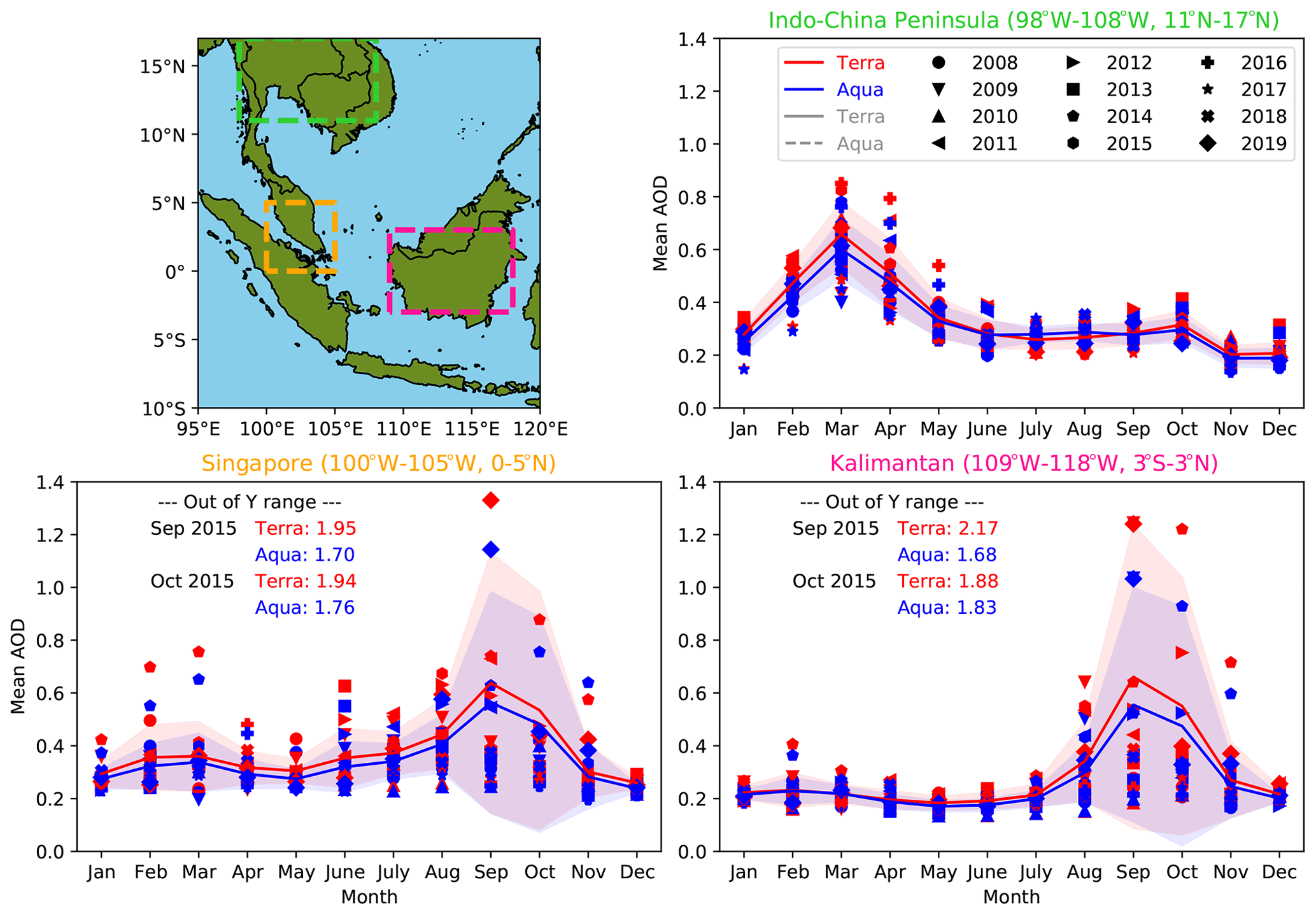
Figure 2MODIS-observed monthly mean AOD averaged over 2008–2019, separately for the three areas shown on the upper left map. The data MOD/MYD08_M3 is 1∘ × 1∘. The shading shows ± SD. The rain belt shifts between ∼ 20∘ N (boreal summer) and ∼ 5∘ S (boreal winter) around this area (e.g., Schneider et al., 2014).
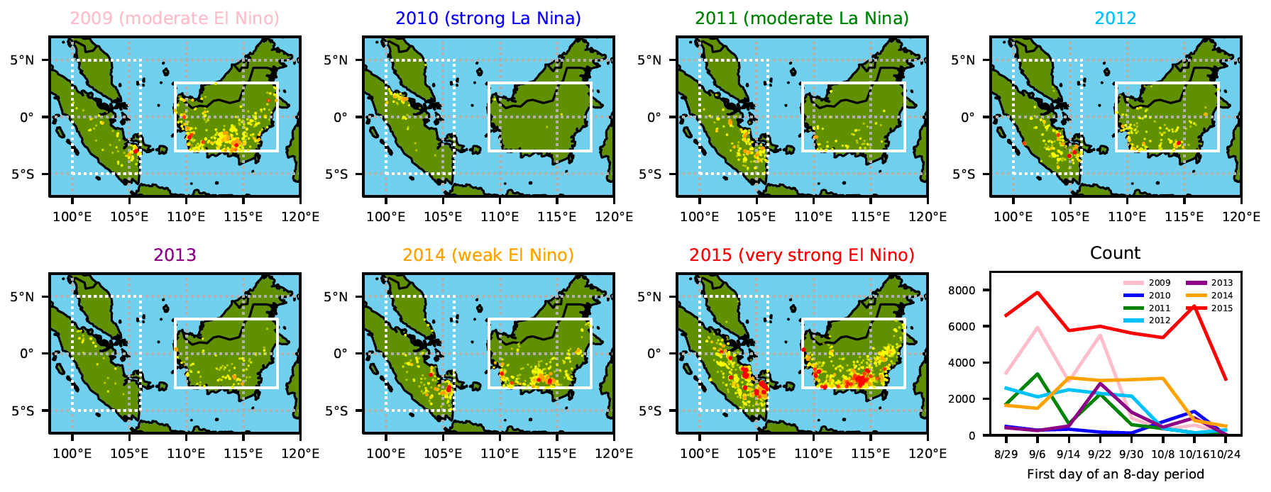
Figure 3Number of fires (with high confidence) within the rectangles according to 1 km MODIS 8 d fire data (MOD/MYD14A2); yellow represents 2–3 counts, orange 4–5 counts, and red >5 counts (the maximum is 16, as Terra and Aqua are counted separately for 8 time frames within September–October). The lower right panel shows the total pixel counts of fires with high confidence within the rectangles.
Microphysical and radiative impacts of fire particles over SEA have been suggested by some observational studies. For instance, Rosenfeld (1999) observed a significant reduction of cloud droplet sizes over the island of Borneo based on TRMM data when clouds were downwind of biomass burning. The investigations of two recent field campaigns over the northern part of SEA by Lin et al. (2013) revealed the detailed chemical and radiative characteristics of fire particles, while their impacts on clouds remained to be clarified. Similarly, the review study by Tsay et al. (2013) summarized the observational findings of the characteristics and the seasonality of fire particles over Indochina. Another review study on aerosols and clouds over SEA by Lin et al. (2014) pointed out that the largest difficulty lies in the simultaneous observation of clouds and aerosols from satellites, as aerosol data get “contaminated” when clouds exist. Therefore, in order to fully understand the connection of fire particles with cloud characteristics, modeling is indispensable.
In spite of the abundance of fire particles, only a few modeling studies have focused on aerosol–cloud interactions (ACIs) over SEA. This may be due to the complexity of multi-scale dynamics over the region that differs quite significantly from season to season and/or year to year or potentially because of a practical reason as a cloud-resolving simulation that covers the entire SEA is computationally expensive. Lee et al. (2014), for example, used the simulations from the GEOS-5 atmospheric general circulation model (AGCM) (resolution 2.5∘ × 2∘) to find a reduction of precipitation over SEA due to both indirect and semi-direct effects of aerosols. Ge et al. (2014), who utilized the Weather Research and Forecasting model (WRF; Skamarock et al., 2008) coupled with Chemistry (WRF-CHEM; Grell et al., 2005) for finer-resolution (27 km) simulations, found a decrease (increase) in cloud fraction during daytime (nighttime) due to the cloud radiative effects of aerosols (including the semi-direct effect) that altered vertical and horizontal flow fields. Simulations in these studies, however, were not on a cloud-resolving scale, which often refers to a horizontal resolution of ∼4 km or finer that does not require parameterization of convections. Hodzic and Duvel (2018, hereinafter HD18) ran cloud-resolving simulations using WRF-CHEM over Borneo for a 40 d period, including the entire month of September, in 2009. According to their simulations, the inclusion of fire particles in the simulations resulted in a reduction of precipitation on island average, but when particle absorptivity was raised, a nighttime enhancement of precipitation was additionally seen. Thus, they concluded that the response of rainfall to aerosol perturbations depended heavily on the absorptivity of fire particles. In the recent study by Lee and Wang (2020, hereinafter LW20), they also used cloud-resolving WRF-CHEM simulations (resolution 5 km) to investigate the impacts of fires on clouds in SEA over a 4-month period from June to September in 2008. Their simulations included not only Borneo but also Sumatra and the Malay and Indochina peninsulas. Even though it is one of a few cloud-resolving modeling studies on ACIs over SEA for such a long period of time, changes of seasons within the time period allowed the dominant flow patterns and emissions to change and hence made it difficult to find ACI signals that were consistent for 4 months. From their in-depth analysis of selected cases, they found a reduction of nocturnal rainfall over western Borneo due mainly to the semi-direct effect of fire particles.
This study aims at further deepening our understanding of ACIs over MC during the peak fire season in the extremely dry year of 2015 (Figs. 1–3) due to the strong El Niño impact. In particular, we address the following questions: (1) how are cloud radiative and microphysical characteristics influenced by fire particles? (2) Does the total amount and/or the diurnal cycle of rainfall change due to fire particles? (3) What do the simulation results imply regarding the indirect impacts of ENSO on precipitation via aerosols? Even though the above studies partly gave answers to some of these questions from their simulations, further investigations and discussions, especially on cloud radiative property changes and ENSO impacts, are essential to fully comprehend ACIs in MC. We seek answers to the questions by running a pair of month-long cloud-resolving WRF-CHEM simulations over MC.
We utilized the WRF-CHEM model version 3.6.1 for the cloud-resolving simulations. The simulation domain is over MC as Fig. 4 shows. The horizontal resolution of this outer domain is 20 km, whose information gets passed to a nested inner domain outlined by the magenta rectangle. This inner domain, which covers the major target region, has a 4 km horizontal resolution and 50 vertical levels. The time steps are 30 and 6 s for the inner and outer domains, respectively.

Figure 4Terrain height (m) within the outer simulation domain, which is outlined by the map. The inner domain is outlined by the magenta rectangle.
Physical and dynamical settings of the simulations are as follows; a simulation with no fire input was initialized at 00:00 UTC on 1 August 2015 by the 1∘ NCEP Final Analysis data (NCEP, NWS, NOAA, U.S. DOC, 2000, GFS-FNL) that also provided 6-hourly boundary conditions to the outer domain. This simulation was run for 31 d for spin-up and continued until the end of September 2015, whereas the other simulation with a fire input started from 1 September with the spun-up chemistry field from the no-fire simulation. Therefore, our analysis period is 1–30 September 2015. Microphysical processes were calculated by the two-moment Morrison scheme (Morrison et al., 2009), but its default upper limit on ice number concentration was removed. Longwave and shortwave radiation processes were calculated by the RRTMG scheme (Iacono et al., 2008), land surface processes by the Unified NOAH land surface model (Tewari et al., 2004), and surface layer processes or planetary boundary layer physics by the Mellor–Yamada–Nakamishi–Niino Level 2.5 scheme (Nakanishi and Niino, 2006, 2009; Olson et al., 2019). Cumulus parameterization, applied solely to the outer domain, was based on the Grell–Freitas ensemble scheme (Grell and Freitas, 2014). 6-hourly grid nudging by the four-dimensional data assimilation (FDDA) was turned on for the outer domain.
Chemistry settings are as follows; emissions were specified by the REanalysis of the TROpospheric chemical composition over the past 40 years (RETRO; Schultz et al., 2008) and the Emission Database for Global Atmospheric Research (EDGAR; http://edgar.jrc.ec.europa.eu, last access: 25 March 2022) via Prep-chem-source (Freitas et al., 2011) version 1.5., except for black carbon, organic carbon, CO, NH3, SO2, NOx (split into 75 % NO and 25 % NO2), PM2.5, and PM10, which were replaced by the 0.25∘-resolution data from the Regional Emission inventory in ASia (REAS; Kurokawa et al., 2013) version 2.1. The month-long spin-up period provided enough time for the concentrations of chemical species to stabilize. As for the calculations of chemical processes, we employed the RADM2 chemical mechanism (Stockwell et al., 1990) with MADE/SORGAM aerosols (Ackermann et al., 1998; Schell et al., 2001). Unfortunately, sea salt emissions needed to be turned off as the appropriate emission option was unavailable. As long as we focus on the comparison between the two simulations, we assumed that this has no impact on our findings. Photolysis was calculated by the Madronich photolysis scheme (Madronich, 1987) and biogenic emissions by the Guenther scheme (Guenther et al., 1994; Simpson et al., 1995).
Under these physical and chemical settings, two simulations were run and compared, with the aim to clarify the impacts of fire particles on clouds and climate. The one with no fire emission is called NOFIRE, and the other with high-resolution fire emissions, based on the Fire INventory from NCAR (Wiedinmyer et al., 2011, FINN) version 1.5, is called FIRE. These fire particles were vertically distributed by the embedded plume-rise model based on Freitas et al. (2007). Other than this fire input, everything else remained identical between the two simulations. It is worth noting here that this choice of fire inventory may have a significant impact on the simulated results; for instance, the Quick Fire Emissions Dataset (QFED; Darmenov and da Silva, 2015) provides a relatively large quantity of particle emissions from fires compared to FINN (e.g., Liu et al., 2020; Pan et al., 2020). On the other hand, the recently published version of FINN (version 2.4) may include an improvement to the FINN dataset that can lead to its large difference from version 1.5 that this study utilized. While the improvements of fire inventories are still ongoing and their comparisons are beyond the scope of this study, the potential impact of using different inventories needs to be kept in mind.
In this chapter, the comparison of the simulations with observations (Sect. 3.1), the comparison of the two simulations (Sect. 3.2), and the comparison of the findings to those in two previous studies (Sect. 3.3) are presented.
3.1 Comparison with observations
In order to assess how realistic the simulations are, here we compare simulated fields against observations. Figure 5 shows the maps of accumulated surface precipitation (mm) between 1 and 30 September 2015 observed by TRMM (Fig. 5a) and simulated by the model (Fig. 5b–c). Despite the general overestimation of the amounts of precipitation in the simulations, the major characteristic distributions are well captured by the model: for instance, large amounts of rainfall in the west of Sumatra (Region 1, red), the southern part of the South China Sea (Region 2, magenta), and in the northern part of Borneo (Region 3, yellow). Our analyses focus on these three regions individually. When daily precipitation patterns are compared, the simulated patterns match the TRMM observations surprisingly well. According to the time series in Fig. 5d–f, the simulations generally capture the observed fluctuations of rainfall rates, especially over Region 2. The discrepancies in the absolute values shown in Fig. 5a–c may be largely due to the lack of ocean dynamics that can lead to more realistic sea surface temperature (SST) distributions. As can be inferred from the effects of ENSO on the amounts of precipitation over MC, SST has significant impacts on convective activities in the tropics (e.g., Graham and Barnett, 1987; Woolnough et al., 2000; Tompkins, 2001). Indeed, MC lies over the tropical warm pool where the Earth's highest SST is observed. Sabin et al. (2013), for example, analyzed the observed data on SST and convective activities around the warm pool and found a tight connection between the two, especially between 26 and 29 ∘C. Estimating SST over MC also faces an additional challenge: the complicatedly distributed but nearly equalized coverages of land and ocean in the area. It hence requires a high-resolution ocean model to accomplish (e.g., Wei et al., 2014). Therefore, the lack of realistic temporal and spatial variations in SST may be one of the reasons why the simulated amounts of rainfall are off, while the spatial distributions and the overall temporal evolution are reasonably well reproduced. Some efforts have already been made to couple WRF/WRF-CHEM with an ocean model as in Warner et al. (2010) and Zhang et al. (2019b). Over MC where the varying sea conditions can strongly influence convective activities, the use of such comprehensive models is more desirable and may lead to more realistic simulations.

Figure 5Accumulated precipitation (mm) for the month of September in 2015 as (a) observed by TRMM and (b) simulated in NOFIRE and (c) FIRE. Red, magenta, and yellow rectangles show the locations of Region 1 (95–101.5∘ W, 5∘ S–7∘ N), Region 2 (101.5–119∘ W, 6.5–9.5∘ N), and Region 3 (108–119∘ W, 0–6.5∘ N), respectively. Time series of TRMM (black, 3-hourly) and simulated (blue and red, hourly) precipitation rates (mm h−1) averaged over each region are shown for (d) Region 1, (e) Region 2, and (f) Region 3.
As for aerosols, there seems to be an overall underestimation of AOD in our simulations on monthly average. Figure 6 shows the maps of monthly mean AOD at 0.55 µm observed by MODIS Terra (Fig. 6a; Aqua shows a similar result) and simulated by the model (Fig. 6b–c), which clearly indicates the underestimation, while the FIRE simulation is closer to the observation as expected. The time series of AODs in Fig. 6d–f also show this underestimation in each region. Nevertheless, horizontal distributions of high-AOD areas are mostly well captured by the FIRE simulations when the daily snapshots of AODs are compared. Figure 7 compares AODs observed at AERONET stations within the simulation domain with those simulated at the nearest grid points. The accuracy of the FIRE simulation varies from station to station, while the general underestimation of AODs by the simulation is seen. The temporal evolution of AODs, however, seems to be reasonably well captured (e.g., Fig. 7d, e, and g). The scale of the AOD values in this figure also needs to be emphasized, as extremely high observed values (e.g., >2.0) are particularly not well captured by the FIRE simulation.
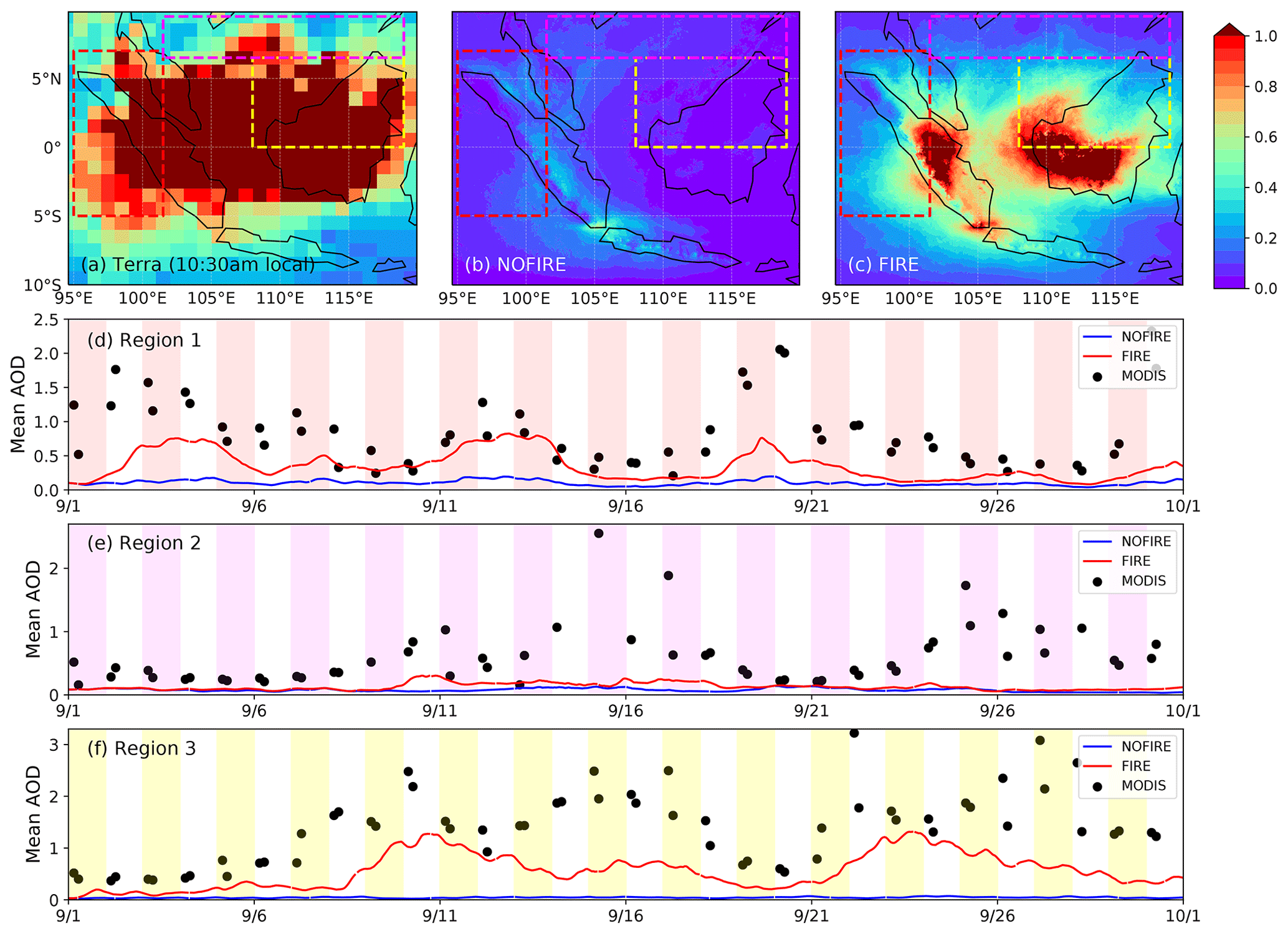
Figure 6Monthly mean AOD at 0.55 µm (a) observed by MODIS Terra (MOD08_D3) and (b) simulated in NOFIRE and (c) FIRE. AOD from MODIS Aqua (MYD08_D3) shows a similar result. The simulated results in (b) and (c) are the averages of AOD snapshots at 03:20 UTC every day, which corresponds to 10:20 Indochina time. Time series of observed (black dots, twice daily) and simulated (blue and red lines, hourly) AODs averaged over each region are shown for (d) Region 1, (e) Region 2, and (f) Region 3. In (d)–(f), both Terra and Aqua are included. Note that the MODIS data were projected onto the UTC time series in (d)–(f), assuming that the data were taken at 10:30 and 13:30 Indochina time.
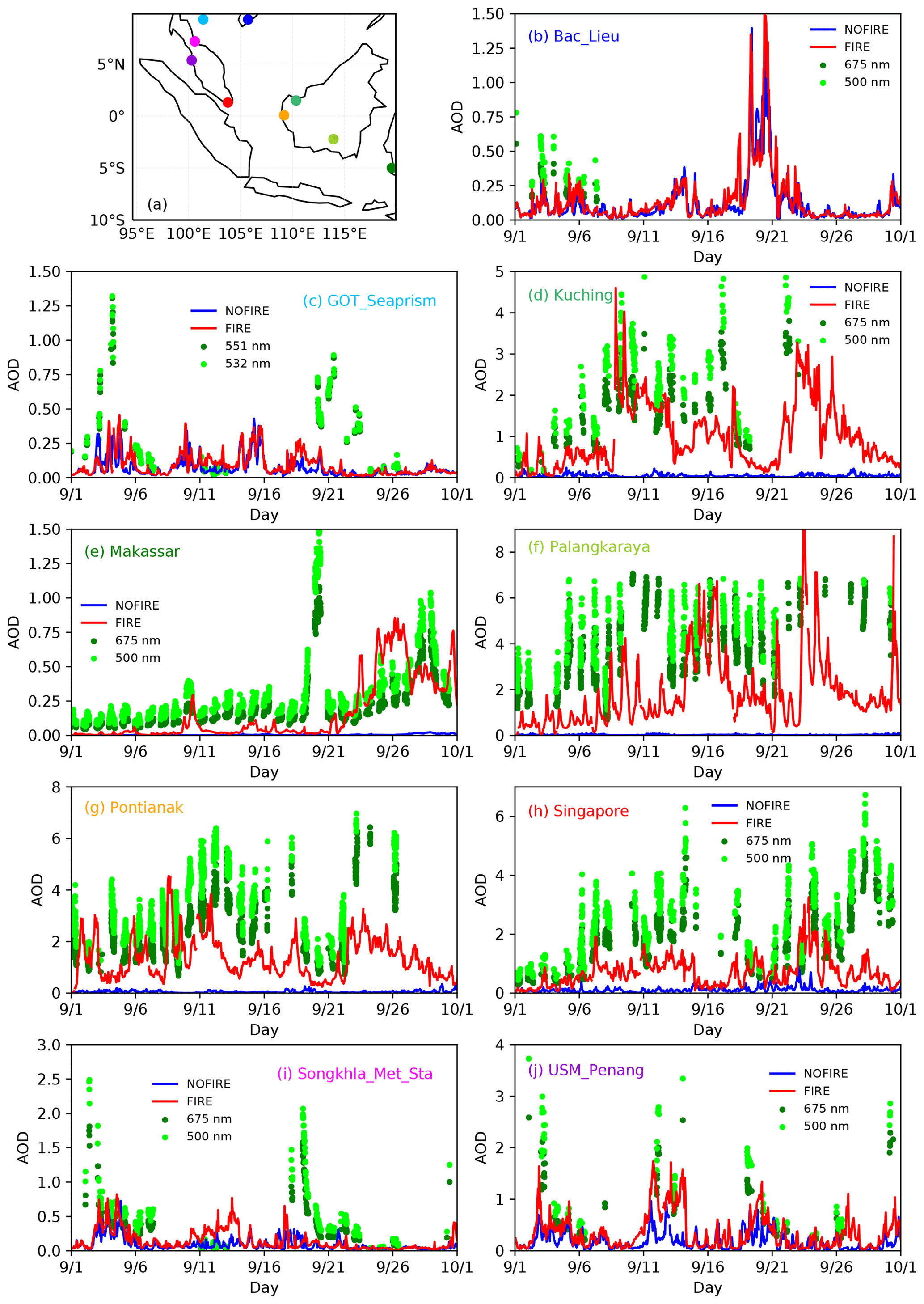
Figure 7(a) Locations of nine AERONET stations whose AOD data for the month of September 2015 are shown in (b)–(j) in green (675 nm) and lime (500 nm). For (c), they are AODs at 551 nm (green) and 532 nm (lime) instead. Red and blue lines are estimated AODs at 550 nm from the FIRE and NOFIRE simulations, respectively.
These comparisons indicate that our simulations capture the overall distributions of rainfall and aerosols, while the amounts of aerosols are likely underestimated. This can be due to the lack of a few large aerosol particles that contribute significantly to AODs because of their large sizes and/or the lack of many small particles. That is, it is possible that FINN greatly underestimated particle emissions from biomass burning, especially in such a year with extreme dryness. It is also plausible that the volume-based calculations of aerosol optical properties from the aerosol abundance lead to the underestimation of AODs, even though the number and mass concentrations of aerosols are realistic. Unfortunately, there is no observation of aerosol number or mass concentrations that can be compared to our simulations. Given the potential for the underestimation of aerosol mass and number, however, it needs to be kept in mind that the effects of fire particles in reality may have been even stronger than what we find from the comparison of the FIRE and NOFIRE simulations presented in the following section.
3.2 FIRE vs. NOFIRE
The inclusion of fire particles led to differences in simulated radiative and microphysical fields. Firstly, their impacts on radiation are discussed. Figure 8a–d show the mean changes in incoming (ground-level) and outgoing (top-of-the-atmosphere) shortwave radiation under clear- and all-sky conditions, respectively. It is clear from this figure that the inclusion of fire particles reduced the solar radiation reaching the ground by scattering and/or absorbing. Such a radiative difference indeed led to lower temperature near the ground in FIRE by a degree or so, as shown in Fig. 8e. The location of this strongest cooling effect coincides with that of the largest reduction in incoming insolation on the ground, implying their connection. At the top of the atmosphere, outgoing shortwave radiation increases in FIRE, particularly over the seas where the surface is dark, due to scattering by fire particles. As a result, albedo increases in the FIRE run (Fig. 8f), although this increase is partly due to the increased cloud optical depth (Fig. 8g); the aerosol direct and indirect effects both worked to increase the overall reflectivity, even though their timing or causal relationship remains uncertain. The reduction in outgoing longwave radiation (OLR) in FIRE (Fig. 8h) indicates that cloud-top heights increased on monthly average. This reduction in OLR suggests that convection was stronger and clouds developed taller in the FIRE run. Although this is contrary to what can be expected from the aerosol radiative effect that reduced the near-ground temperature and worked to stabilize the atmosphere, we show next that convection became stronger in the FIRE run and increased the amount of rainfall.
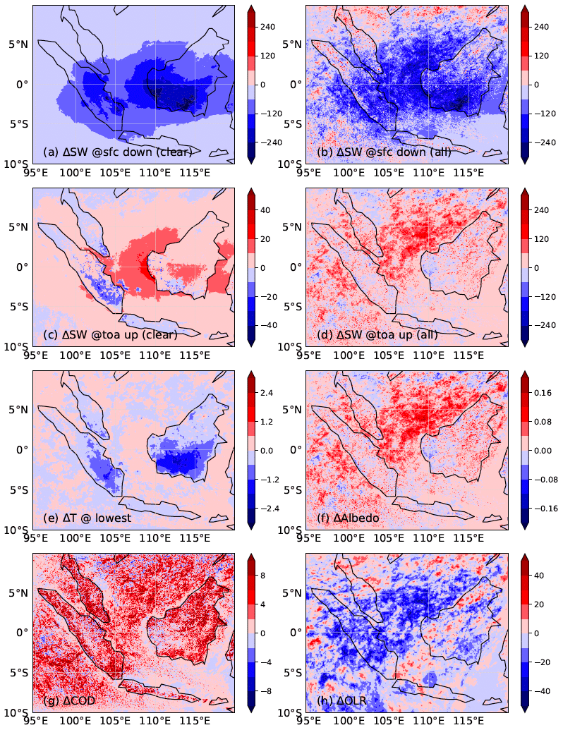
Figure 8Simulated monthly mean differences (FIRE−NOFIRE) in (a) clear- and (b) all-sky downward shortwave radiation on the ground (Wm −2), (c) clear- and (d) all-sky upward shortwave radiation at the top of the atmosphere (Wm −2), (e) temperature at the lowest model level (K), (f) albedo (unitless), (g) estimated cloud optical depth (unitless), and (h) OLR (Wm −2). These are the averages of differences at 06:00 UTC (around local midday) every day in the month of September 2015.
The differences in rainfall between NOFIRE and FIRE, shown in Fig. 9a, clearly indicate the enhancement of precipitation in the FIRE simulation over the simulation domain. The maximum increase amounts to 645.4 (millimeters per month) and the domain-mean difference is +25.9 (millimeters per month). Based on our analyses, this rainfall difference is a result of a modified chain of microphysical processes rather than dynamical differences: as mentioned above, the aerosol radiative effect seemed to have stabilized the atmosphere, which has the opposite effect to the invigoration of convection. Therefore, it is fair to state that the enhanced rainfall was triggered by the microphysical effect of fire particles. The rest of this subsection is dedicated to explaining the microphysical mechanisms that made rainfall increase and clouds become taller and more reflective in the FIRE simulation as presented above.
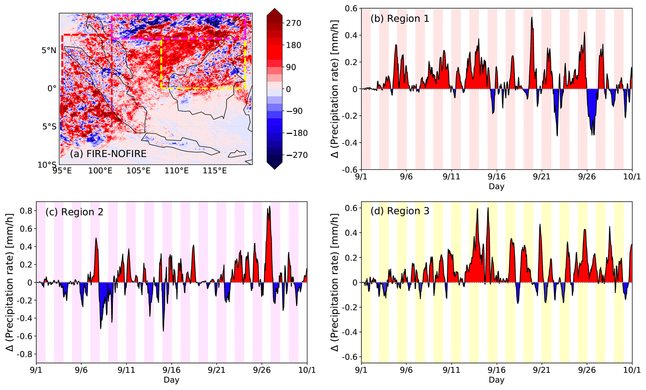
Figure 9(a) Difference (FIRE−NOFIRE) in accumulated precipitation (mm) over the month of September. (b–d) Time series of regional mean precipitation rate (mm h−1) differences (FIRE−NOFIRE) in (b) Region 1, (c) Region 2, and (d) Region 3.
According to Fig. 9b–d, the amount of rainfall clearly increases in the FIRE simulation over Region 1 and Region 3, which both include a large portion of land, whereas the precipitation change is equally positive and negative over Region 2, which is over a sea. In order to understand at what time this increase occurs in a day, regional mean differences (FIRE−NOFIRE) in hourly precipitation rate (mm h−1) are plotted in Fig. 10 (left column), along with their monthly means (magenta). This analysis shows that the increase occurs at 12:00–04:00 UTC on average, which is from evening to morning in local time. No decrease is seen at other times. To confirm that this increase in nocturnal rainfall is not due to a single passage of a large convective system, the numbers of days with regional mean increase (+1, red, FIRE > NOFIRE) and decrease (−1, blue, FIRE < NOFIRE) are counted every hour in Fig. 10 (right column). Combining the plots in Fig. 10, it is clear that there are many days when precipitation rates increase in FIRE at night (right column), which all contribute to the increase in mean precipitation rates at 12:00–04:00 UTC (left column, magenta). As no rainfall reduction is seen for the rest of the day, we conclude that these precipitation increases over Regions 1 and 3 are an enhancement of nocturnal precipitation rather than a temporal shifting of a diurnal cycle. When monthly mean mass mixing ratios of hydrometeors are compared between FIRE and NOFIRE (Figs. 11 and A1), an increase in all hydrometeor masses in FIRE is apparent, particularly that of snow and graupel over Regions 1 and 3. It is also clear that the latitudinal (Region 1) or longitudinal (Regions 2 and 3) patterns of the rain, snow, and graupel masses correspond very well with each other, implying the significant contribution of melted snow and graupel to rain mass. Furthermore, the absolute difference values shown in Figs. 11 and A1 are on the order of 0.01 (g m−3) for rain, snow, and graupel in all three regions, whereas those for cloud droplets are merely 0.001 (g m−3). Thus, surface rainfall seems to largely stem from melted snow and graupel. As more aerosol particles exist in the FIRE simulation, the number of smaller droplets increases. This initiated a chain of altered microphysical processes that led to the increase in snow production, which is essential for subsequent graupel production. Further analyses of microphysical process rates (Fig. A2) show cloud features that are consistent with both of the hypotheses that (i) more cloud droplets remain in air without raining out and later freeze aloft to form more ice crystals that are essential for more snow formation in FIRE, and (ii) the increased mass and number of cloud droplets in the FIRE simulation set a more favorable condition for efficient snow and graupel production in clouds, such as through droplet accretion by snow (Fig. A2g–i). Both of these paths may have concurrently played a role in producing more snow in the FIRE simulation. Once snow mass increases, graupel mass also increases as they form on snow by riming. As for the invigoration of convection signified by the increased rainfall and cloud-top height, our analysis has revealed that the increased latent heat release is predominantly through increased condensation rather than increased freezing; Fig. A3 shows the estimated rates of maximum latent heat release following droplet activation and freezing. According to these estimates, convection was likely invigorated more by increased condensation and less so by increased freezing. This result agrees with what was shown by Fan et al. (2018) and Lebo (2018). As a result of the enhanced condensation, the maximum supersaturation is lowered inside convection in FIRE (Fig. A4). It is also likely that, once convection gets invigorated, stronger downdrafts can in turn induce stronger convection, creating a positive feedback. This may have played a role in the invigorated convections in our FIRE simulation.
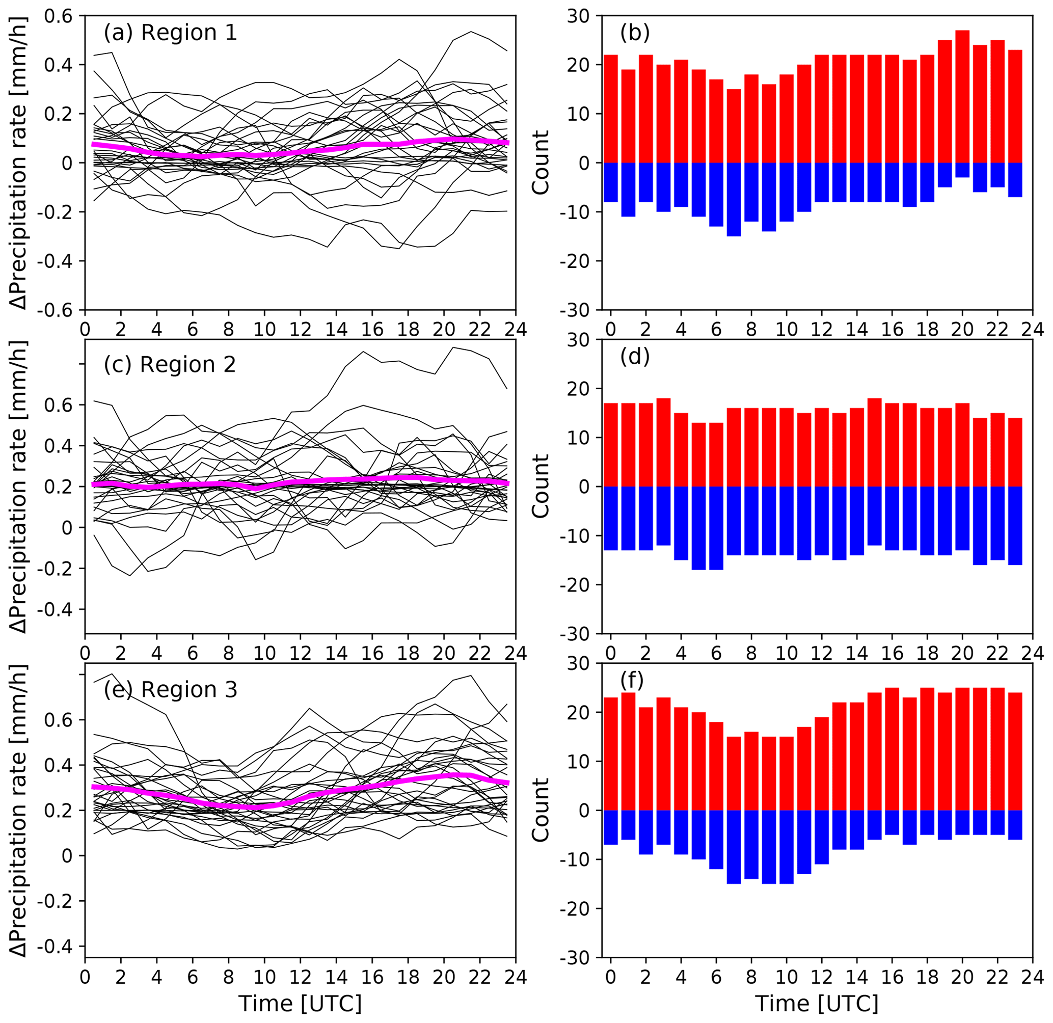
Figure 10(a, c, e) FIRE−NOFIRE differences in hourly precipitation rate (mm h−1) each day in September (black) and their monthly average (magenta). (b, d, f) Raw counts of increased (+1, red) or decreased (−1, blue) hourly rainfall rates (FIRE−NOFIRE). All are averages over (a, b) Region 1, (c, d) Region 2, and (e, f) Region 3.
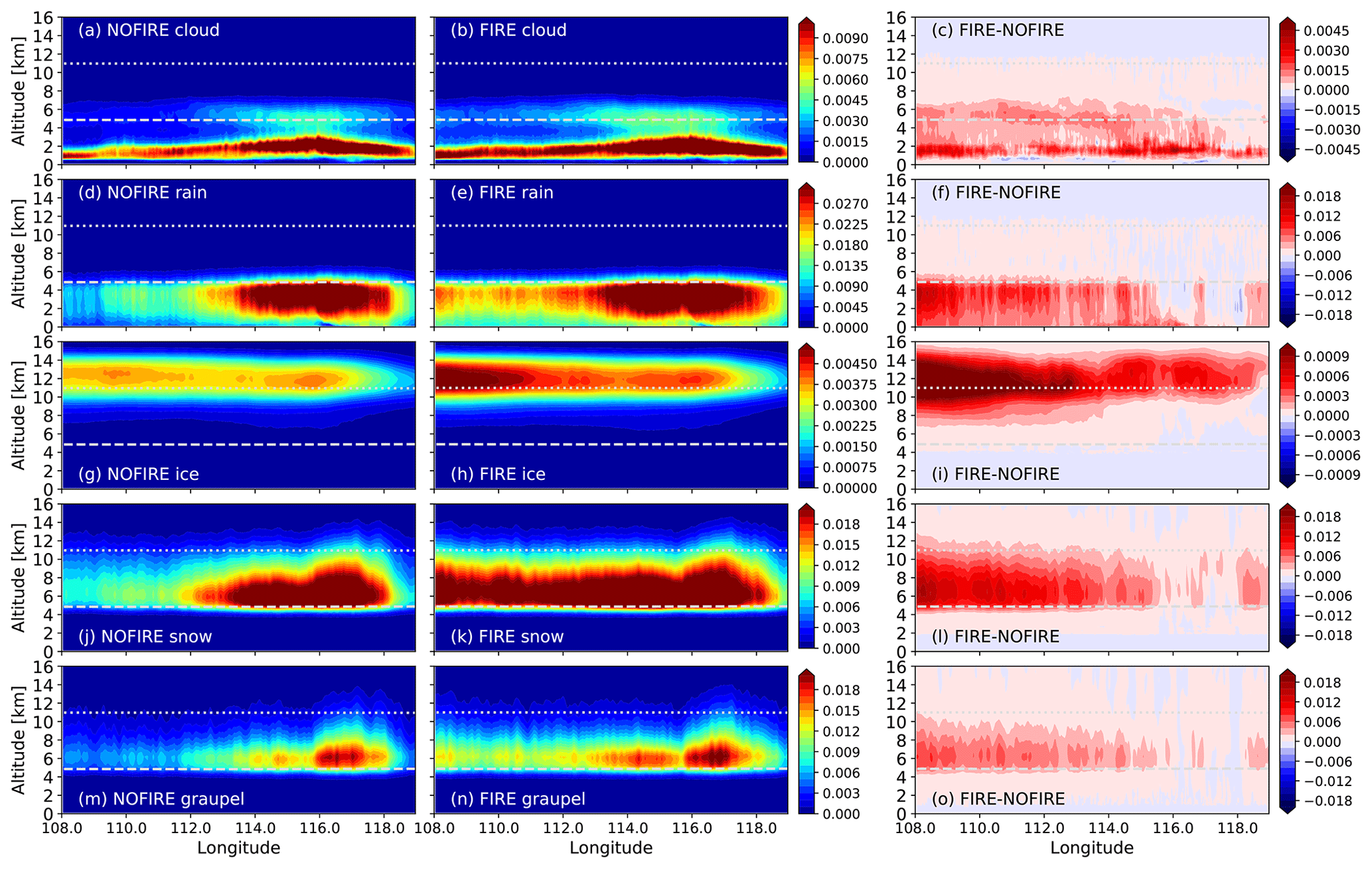
Figure 11Monthly and meridional mean mass concentrations (g m−3) of (a, b) liquid cloud, (d, e) rain, (g, h) ice, (j, k) snow, and (m, n) graupel in (a, d, g, j, m) NOFIRE and (b, e, h, k, n) FIRE over Region 3. These are averages inside grid boxes wherein each hydrometeor mass >0. Respective differences (FIRE−NOFIRE) are shown in the rightmost column. The dashed and dotted lines are temporally and meridionally averaged 0 and −40 ∘C isotherms, respectively. See Fig. A1 for equivalent difference figures for Regions 1 and 2.
Areas with increased cloud optical depth (Fig. 8g) overlap with areas of increased droplet number concentrations (over land) and areas of increased ice mass (over sea) based on Fig. 12. This suggests the direct impacts of fire particles on cloud droplets over land (i.e., source region) and their propagated impacts over seas on cloud reflectivity via ice. As for cloud-top heights, the areas of decreased OLR (Fig. 8h) correspond well with the areas of increased ice (Fig. 12d–f), mostly over seas. This increased mass of ice crystals is likely due to the hypothesis (i) stated above, which applies to convective clouds that can eventually dissipate into more stratiform anvil clouds and drift in the atmosphere for an extended period of time. Such aerosol-induced changes in stratiform anvil clouds, namely their extended lifetime and heightened cloud top, have been reported in previous studies (e.g., Fan et al., 2013), even though these changes can be independent of the invigoration of convection. The increased ice mass indicates increased latent heat release in FIRE through freezing and riming, which is consistent with the higher cloud tops. Thus, an increase in fire particles triggered the changes in microphysical process rates that ultimately modified the cloud radiative properties.
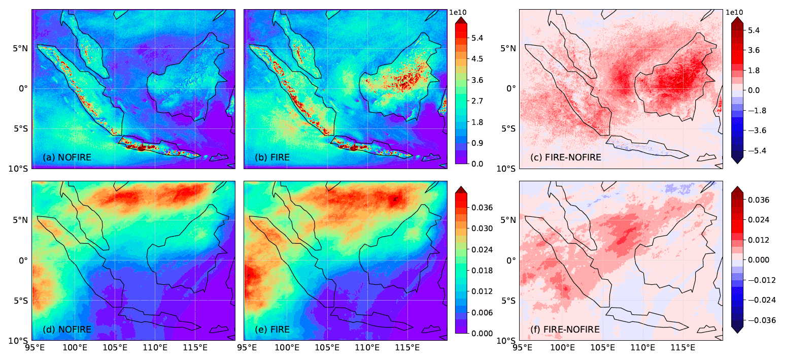
Figure 12Monthly mean column-integrated (a, b) cloud droplet number (m−2) and (d, e) ice mass (kg m−2) in (a, d) NOFIRE and (b, e) FIRE. Differences are shown in (c) and (f).
These microphysically driven changes in cloud properties have some implications for climate. The invigoration of convective clouds produces more rainfall and hence facilitates the energy exchange between the surface and the upper atmosphere. Interestingly, the increase in fire particles in the atmosphere is partly dependent on the amount of precipitation; the year 2015 was particularly dry and had exceptionally high AODs (Fig. 2) due to the lack of rainfall (Fig. 1). Although the amount of increased rainfall in FIRE is not as much as interannual differences, our simulations showed the effect of fire particles to slightly compensate for the lack of rainfall in the year 2015.
3.3 Comparison with previous studies
Here we compare the results in this study with those from HD18 and LW20. The objective of this subsection is to clarify the differences in the overall impacts of ACIs among the three studies, particularly in the surface rainfall changes. As simulation settings differ among the three, only the signs of the rainfall change are concerned rather than its magnitude or physical mechanism. The simulation period was mostly September in HD18 and 4 months from June to September in LW20. The month of September is therefore the common period of interest among these studies and the current work. The ENSO phase, however, differs among the three: very strong El Niño in 2015 (this study), moderate El Niño in 2009 (HD18), and weak La Niña in 2008 (LW20), according to the 3-month running mean Oceanic Niño Index. Although the simulation resolutions are more or less the same cloud-resolving scale for the three (i.e., 4 or 5 km), the simulation domain contains both Indochina and MC in LW20, only MC in this study, and only Borneo in HD18. With these differences in mind, the findings of rainfall changes due to fires over Borneo are compared in this subsection.
Our results show the increase in nocturnal rainfall over Borneo (i.e., Region 3) due to the intensification of convective clouds through microphysical processes. The direct and semi-direct effects of aerosols were small. In HD18, however, the inclusion of fires reduced the rainfall from late afternoon to evening (see their Fig. 5) for radiative (stabilization of the atmosphere) and microphysical (locally vary) reasons. As for LW20, rainfall slightly increased during daytime but decreased during nighttime when fires were included (see their Fig. 10). LW20 concluded that it was likely due to the semi-direct effect of aerosols, which reinforced the sea breeze during the day but weakened the land breeze at night. Over the same region and same month, these studies have varying results for the fire-induced rainfall change and its mechanism. We attribute these differences to (a) microphysical parameterizations and their sensitivities to aerosol perturbations, (b) settings of aerosol properties, such as absorptivity and size distributions, that would affect the sign and/or magnitude of aerosol radiative effects, and (c) the interannual variability of the dominant regional weather pattern that prevails over SEA, likely varying with the ENSO phase. As for (a) and partly for (b), both LW20 and this study used the Morrison scheme (Morrison et al., 2009), but the removal of the default upper limit on ice number concentrations in this study may have increased the sensitivity of clouds to aerosol perturbations. HD18 utilized the two-moment scheme by Thompson and Eidhammer (2014) that separates aerosols into water-friendly and ice-friendly and activates a fraction of water-friendly aerosols based on a lookup table. These differences in the calculations of microphysical processes must have a considerable influence on the simulated results of the fire effects. The additional factor of (c) may further complicate the interpretation of the differences among simulations. Therefore, comparisons of simulations with a consistent microphysics scheme or the same ENSO phase are required for fully clarifying the role of fire particles in clouds or the effects of ENSO phases on ACIs over the region.
We have used two cloud-resolving WRF-CHEM simulations to reveal the impacts of fire particles on cloud microphysics and radiation over MC for the month of September in 2015, when extremely high AODs were observed. Our month-long FIRE simulation with fire particles showed more reflective and taller clouds than those in the NOFIRE simulation. The amount of precipitation was also larger in the FIRE simulation. All of these features suggest the invigoration of convection by fire particles. Based on our further analyses, the increased mass of snow seemed to be particularly responsible for the increased rainfall, whereas the changes in cloud-top height and reflectivity stemmed mainly from increased ice crystals that are more reflective and longer-lived than snow. The changes in microphysical process rates were all initiated by a simple increase in aerosol number concentrations, which in turn triggered a chain of modified microphysical processes such as increased freezing of smaller ice crystals aloft and thermodynamic responses. Although the magnitude of the differences between FIRE and NOFIRE is not comparable to interannual differences, we conclude that the intensification of convection by fire particles acted to partly compensate for the lack of rainfall for the month of September 2015. These findings answer the three scientific questions posed for this study in the Introduction.
It is of a profound interest to understand the interannual variability of aerosol effects potentially influenced by ENSO, which is commonly believed to be a major driver for convective activities and also a critical factor behind biomass burning in SEA. To explore this issue, we have compared our simulations with two previous studies, perhaps the only other cloud-resolving, month-long simulations available hitherto over the region but for years in different ENSO phases. Convective systems in our simulations displayed the invigoration effect by fire particles that the two studies did not show. Nevertheless, many questions still remain unanswered. For instance, do smaller quantities of aerosols in other years simply exert the weaker invigoration effect that was presented in this study? Or do even small quantities of aerosols have an equivalently strong invigoration effect if the background condition is always pristine, unlike the aerosol-loaded year of 2015? Does the aerosol semi-direct effect play a stronger role in other years or depending on the aerosol settings in simulations? Are aerosol effects completely different under different weather regimes? Although it was out of the scope of this paper, recent studies such as Zhang et al. (2019a) have shown the potential importance of heat effects of fires for convective clouds; they found strengthening of convection by the heat effects and therefore significant changes in subsequent cloud properties in their simulations. In the region of our interest, how much the heat effects of fires enhance the invigoration of convection could definitely be examined in the future. Furthermore, do our simulation results depend on the fire inventory used for the simulations? The answers to all of these questions will be sought in our future work.
This Appendix provides additional figures that support the contents of the paper.

Figure A1Same as (c, f, i, l, o) in Fig. 11 but for (a, c, e, g, i) Region 1 and (b, d, f, h, j) Region 2. Note that it is a zonal mean, rather than a meridional mean, for Region 1.
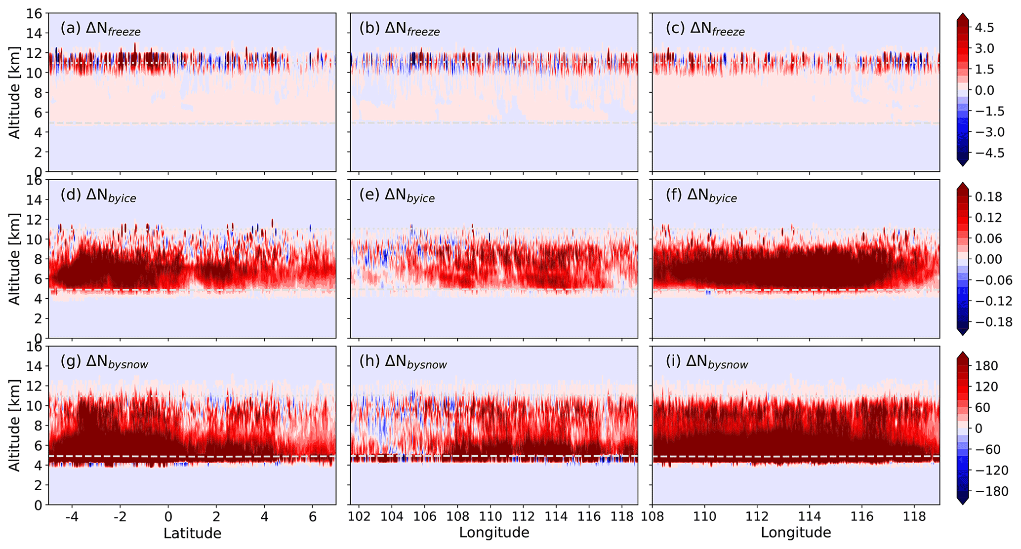
Figure A2Differences (FIRE−NOFIRE) in monthly and zonal (Region 1) or meridional (Regions 2 and 3) mean rates (kg−1 s−1) of droplet number changes via (a–c) cloud droplet freezing, (d–f) droplet accretion by ice, and (g–i) droplet accretion by snow in (a, d, g) Region 1, (b, e, h) Region 2, and (c, f, i) Region 3. These are averages inside grid boxes with rates >0.

Figure A3Differences (FIRE−NOFIRE) in the estimated rate of maximum latent heat release (J kg−1 s−1) following (a, b, c) droplet activation and (d, e, f) droplet freezing in (a, d) Region 1, (b, e) Region 2, and (c, f) Region 3. These were estimated from newly activated droplet number concentration (kg−1), time step (s), droplet freezing rate (kg−1 s−1), and cloud droplet and ice effective radii rc and ri. Since newly formed droplets and ice crystals are typically smaller than rc and ri, respectively, these are the maximum estimates. Note the difference in the scale of the color bars.
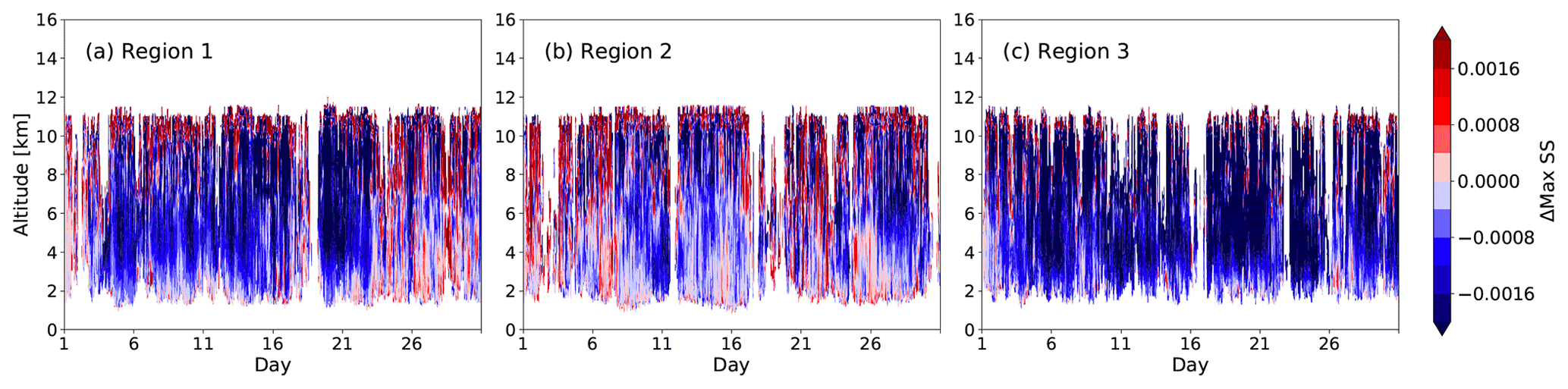
Figure A4Differences (FIRE−NOFIRE) in maximum supersaturation Smax averaged within each region, only sampled where updraft ≥5 ms−1 and Smax>0.
The source codes of the WRF-CHEM model used in the study are publicly available on the University Corporation for Atmospheric Research (UCAR) website at https://www2.mmm.ucar.edu/wrf/users/download/get_source.html (UCAR, 2022a). GFS-FNL data (NCEP, NWS, NOAA, U.S. DOC, 2000) are also available on the UCAR website at https://doi.org/10.5065/D6M043C6. As for the emission datasets, FINN version 1.5 data are available on the UCAR website at https://www.acom.ucar.edu/Data/fire/ (UCAR, 2022b). REAS version 2.1 data are made available by the National Institute for Environmental Studies (NIES) in Japan at https://www.nies.go.jp/REAS/ (NIES, 2022). Prep-chem-source can be directly downloaded from the National Oceanic and Atmospheric Administration (NOAA) website at ftp://aftp.fsl.noaa.gov/divisions/taq/global_emissions/ (last access: 25 March 2022). As for the observational datasets, the Oceanic Niño Index can be found on NOAA's National Weather Service website at https://origin.cpc.ncep.noaa.gov/products/analysis_monitoring/ensostuff/ONI_v5.php (NOAA, 2022). MODIS AOD (https://doi.org/10.5067/MODIS/MOD08_M3.061 and https://doi.org/10.5067/MODIS/MYD08_M3.061, Platnick et al., 2022a; https://doi.org/10.5067/MODIS/MOD08_D3.061 and https://doi.org/10.5067/MODIS/MYD08_D3.061, Platnick et al., 2022b) and fire (https://doi.org/10.5067/MODIS/MOD14A2.006, Giglio and Justice, 2015a; https://doi.org/10.5067/MODIS/MYD14A2.006, Giglio and Justice, 2015b) data are all made available by the National Aeronautics and Space Administration (NASA) at https://ladsweb.modaps.eosdis.nasa.gov/ (last access: 25 March 2022). AERONET data are also available on NASA's website at https://aeronet.gsfc.nasa.gov/ (NASA, 2022). TRMM data (Tropical Rainfall Measuring Mission, 2011) are also available on the NASA website at https://doi.org/10.5067/TRMM/TMPA/MONTH/7. Readers interested in the specific modifications made to the WRF-CHEM source code for this study can contact the corresponding author.
AT and CW conceptualized the research theme and designed the simulations. AT ran the simulations, analyzed and visualized the results, and wrote the original draft of the paper. CW supervised the overall work and contributed to the preparation of the submitted paper.
The contact author has declared that neither they nor their co-authors have any competing interests.
Publisher's note: Copernicus Publications remains neutral with regard to jurisdictional claims in published maps and institutional affiliations.
This work is a part of the Make Our Planet Great Again project and is funded by the L'Agence National de la Recherche (ANR) of France under the Programme d'Investissements d'Avenir (ANR-18-MOPGA-003 EUROACE) and co-funded by the French region of Occitanie. We appreciate the computational support provided by the Institute for Development and Resources in Intensive Scientific Computing (IDRIS) and the Grand Équipement National de Calcul Intensif (GENCI) for the numerical simulations in this work. We thank all the corresponding institutions for making their data products available for this study. We also thank the two anonymous reviewers for their insightful comments and suggestions that allowed us to significantly improve the paper.
This research has been supported by the Agence Nationale de la Recherche (grant no. ANR-18-MOPGA-003 EUROACE) and the French region of Occitanie.
This paper was edited by Toshihiko Takemura and reviewed by two anonymous referees.
Ackermann, I. J., Hass, H., Memmesheimer, M., Ebel, A., Binkowski, F. S., and Shankar, U.: Modal aerosol dynamics model for Europe: Development and first applications, Atmos. Environ., 32, 2981–2999, https://doi.org/10.1016/S1352-2310(98)00006-5, 1998. a
Darmenov, A. S. and da Silva, A.: The Quick Fire Emissions Dataset (QFED): Documentation of versions 2.1, 2.2 and 2.4, Technical Report Series on Global Modeling and Data Assimilation, NASA/TM-2015-104606/Vol. 38, https://gmao.gsfc.nasa.gov/pubs/docs/Darmenov796.pdf (last access: 25 March 2022), 2015. a
Fan, J., Leung, L. R., Rosenfeld, D., Chen, Q., Li, Z., Zhang, J., and Yan, H.: Microphysical effects determine macrophysical response for aerosol impacts on deep convective clouds, P. Natl. A. Sci. USA, 110, E4581–E4590, https://doi.org/10.1073/pnas.1316830110, 2013. a
Fan, J., Rosenfeld, D., Zhang, Y., Giangrande, S. E., Li, Z., Machado, L. A. T., Martin, S. T., Yang, Y., Wang, J., Artaxo, P., Barbosa, H. M. J., Braga, R. C., Comstock, J. M., Feng, Z., Gao, W., Gomes, H. B., Mei, F., Pöhlker, C., Pöhlker, M. L., Pöschl, U., and de Souza, R. A. F.: Substantial convection and precipitation enhancements by ultrafine aerosol particles, Science, 359, 411–418, https://doi.org/10.1126/science.aan8461, 2018. a
Freitas, S. R., Longo, K. M., Chatfield, R., Latham, D., Silva Dias, M. A. F., Andreae, M. O., Prins, E., Santos, J. C., Gielow, R., and Carvalho Jr., J. A.: Including the sub-grid scale plume rise of vegetation fires in low resolution atmospheric transport models, Atmos. Chem. Phys., 7, 3385–3398, https://doi.org/10.5194/acp-7-3385-2007, 2007. a
Freitas, S. R., Longo, K. M., Alonso, M. F., Pirre, M., Marecal, V., Grell, G., Stockler, R., Mello, R. F., and Sánchez Gácita, M.: PREP-CHEM-SRC – 1.0: a preprocessor of trace gas and aerosol emission fields for regional and global atmospheric chemistry models, Geosci. Model Dev., 4, 419–433, https://doi.org/10.5194/gmd-4-419-2011, 2011. a
Ge, C., Wang, J., and Reid, J. S.: Mesoscale modeling of smoke transport over the Southeast Asian Maritime Continent: coupling of smoke direct radiative effect below and above the low-level clouds, Atmos. Chem. Phys., 14, 159–174, https://doi.org/10.5194/acp-14-159-2014, 2014. a
Giglio, L. and Justice, C.: MOD14A2 MODIS/Terra Thermal Anomalies/Fire 8-Day L3 Global 1 km SIN Grid V006, NASA EOSDIS Land Processes DAAC [data set], https://doi.org/10.5067/MODIS/MOD14A2.006, 2015a. a
Giglio, L. and Justice, C.: MYD14A2 MODIS/Aqua Thermal Anomalies/Fire 8-Day L3 Global 1 km SIN Grid V006, NASA EOSDIS Land Processes DAAC [data set], https://doi.org/10.5067/MODIS/MYD14A2.006, 2015b. a
Graham, N. E. and Barnett, T. P.: Sea Surface Temperature, Surface Wind Divergence, and Convection over Tropical Oceans, Science, 238, 657–659, https://doi.org/10.1126/science.238.4827.657, 1987. a
Grell, G. A. and Freitas, S. R.: A scale and aerosol aware stochastic convective parameterization for weather and air quality modeling, Atmos. Chem. Phys., 14, 5233–5250, https://doi.org/10.5194/acp-14-5233-2014, 2014. a
Grell, G. A., Peckham, S. E., Schmitz, R., McKeen, S. A., Frost, G., Skamarock, W. C., and Eder, B.: Fully coupled “online” chemistry within the WRF model, Atmos. Environ., 39, 6957–6975, https://doi.org/10.1016/j.atmosenv.2005.04.027, 2005. a
Guenther, A., Zimmerman, P., and Wildermuth, M.: Natural volatile organic compound emission rate estimates for U.S. woodland landscapes, Atmos. Environ., 28, 1197–1210, https://doi.org/10.1016/1352-2310(94)90297-6, 1994. a
Hodzic, A. and Duvel, J. P.: Impact of Biomass Burning Aerosols on the Diurnal Cycle of Convective Clouds and Precipitation Over a Tropical Island, J. Geophys. Res.-Atmos., 123, 1017–1036, https://doi.org/10.1002/2017JD027521, 2018. a
Iacono, M. J., Delamere, J. S., Mlawer, E. J., Shephard, M. W., Clough, S. A., and Collins, W. D.: Radiative forcing by long-lived greenhouse gases: Calculations with the AER radiative transfer models, J. Geophys. Res.-Atmos., 113, D13103, https://doi.org/10.1029/2008JD009944, 2008. a
Kurokawa, J., Ohara, T., Morikawa, T., Hanayama, S., Janssens-Maenhout, G., Fukui, T., Kawashima, K., and Akimoto, H.: Emissions of air pollutants and greenhouse gases over Asian regions during 2000–2008: Regional Emission inventory in ASia (REAS) version 2, Atmos. Chem. Phys., 13, 11019–11058, https://doi.org/10.5194/acp-13-11019-2013, 2013. a
Lebo, Z.: A Numerical Investigation of the Potential Effects of Aerosol-Induced Warming and Updraft Width and Slope on Updraft Intensity in Deep Convective Clouds, J. Atmos. Sci., 75, 535–554, https://doi.org/10.1175/JAS-D-16-0368.1, 2018. a
Lee, D., Sud, Y. C., Oreopoulos, L., Kim, K.-M., Lau, W. K., and Kang, I.-S.: Modeling the influences of aerosols on pre-monsoon circulation and rainfall over Southeast Asia, Atmos. Chem. Phys., 14, 6853–6866, https://doi.org/10.5194/acp-14-6853-2014, 2014. a
Lee, H.-H. and Wang, C.: The impacts of biomass burning activities on convective systems over the Maritime Continent, Atmos. Chem. Phys., 20, 2533–2548, https://doi.org/10.5194/acp-20-2533-2020, 2020. a
Lenssen, N. J. L., Goddard, L., and Mason, S.: Seasonal Forecast Skill of ENSO Teleconnection Maps, Weather Forecast., 35, 2387–2406, https://doi.org/10.1175/WAF-D-19-0235.1, 2020. a
Lin, N.-H., Tsay, S.-C., Maring, H. B., Yen, M.-C., Sheu, G.-R., Wang, S.-H., Chi, K. H., Chuang, M.-T., Ou-Yang, C.-F., Fu, J. S., Reid, J. S., Lee, C.-T., Wang, L.-C., Wang, J.-L., Hsu, C. N., Sayer, A. M., Holben, B. N., Chu, Y.-C., Nguyen, X. A., Sopajaree, K., Chen, S.-J., Cheng, M.-T., Tsuang, B.-J., Tsai, C.-J., Peng, C.-M., Schnell, R. C., Conway, T., Chang, C.-T., Lin, K.-S., Tsai, Y. I., Lee, W.-J., Chang, S.-C., Liu, J.-J., Chiang, W.-L., Huang, S.-J., Lin, T.-H., and Liu, G.-R.: An overview of regional experiments on biomass burning aerosols and related pollutants in Southeast Asia: From BASE-ASIA and the Dongsha Experiment to 7-SEAS, Atmos. Environ., 78, 1–19, https://doi.org/10.1016/j.atmosenv.2013.04.066, 2013. a
Lin, N.-H., Sayer, A. M., Wang, S.-H., Loftus, A. M., Hsiao, T.-C., Sheu, G.-R., Hsu, N. C., Tsay, S.-C., and Chantara, S.: Interactions between biomass-burning aerosols and clouds over Southeast Asia: Current status, challenges, and perspectives, Environ. Pollut., 195, 292–307, https://doi.org/10.1016/j.envpol.2014.06.036, 2014. a, b
Liu, T., Mickley, L. J., Marlier, M. E., DeFries, R. S., Khan, M. F., Latif, M. T., and Karambelas, A.: Diagnosing spatial biases and uncertainties in global fire emissions inventories: Indonesia as regional case study, Remote Sens. Environ., 237, 111557, https://doi.org/10.1016/j.rse.2019.111557, 2020. a
Madronich, S.: Photodissociation in the atmosphere: 1. Actinic flux and the effects of ground reflections and clouds, J. Geophys. Res.-Atmos., 92, 9740–9752, https://doi.org/10.1029/JD092iD08p09740, 1987. a
Morrison, H., Thompson, G., and Tatarskii, V.: Impact of Cloud Microphysics on the Development of Trailing Stratiform Precipitation in a Simulated Squall Line: Comparison of One- and Two-Moment Schemes, Mon. Weather Rev., 137, 991–1007, https://doi.org/10.1175/2008MWR2556.1, 2009. a, b
Nakanishi, M. and Niino, H.: An Improved Mellor–Yamada Level-3 Model: Its Numerical Stability and Application to a Regional Prediction of Advection Fog, Bound.-Lay. Meteorol., 119, 397–407, https://doi.org/10.1007/s10546-005-9030-8, 2006. a
Nakanishi, M. and Niino, H.: Development of an Improved Turbulence Closure Model for the Atmospheric Boundary Layer, J. Meteorol. Soc. Jpn., 87, 895–912, https://doi.org/10.2151/jmsj.87.895, 2009. a
NASA: AERONET, https://aeronet.gsfc.nasa.gov/, last access: 25 March 2022. a
NCEP, NWS, NOAA, U.S. DOC: NCEP FNL Operational Model Global Tropospheric Analyses, continuing from July 1999, Research Data Archive at the National Center for Atmospheric Research, Computational and Information Systems Laboratory, Boulder, CO, U.S.A., NCEP, NWS, NOAA, U.S. DOC [data set], https://doi.org/10.5065/D6M043C6, 2000. a, b
NIES: Regional Emission inventory in ASia (REAS) Data Download Site, https://www.nies.go.jp/REAS/, last access: 25 March 2022. a
NOAA: Cold and Warm Episodes by Season, https://origin.cpc.ncep.noaa.gov/products/analysis_monitoring/ensostuff/ONI_v5.php, last access: 25 March, 2022. a
Olson, J. B., Kenyon, J. S., Angevine, W. A., Brown, J. M., Pagowski, M., and Sušelj, K.: A Description of the MYNN-EDMF Scheme and the Coupling to Other Components in WRF–ARW, NOAA Technical Memorandum OAR GSD; 61, https://doi.org/10.25923/n9wm-be49, 2019. a
Pan, X., Ichoku, C., Chin, M., Bian, H., Darmenov, A., Colarco, P., Ellison, L., Kucsera, T., da Silva, A., Wang, J., Oda, T., and Cui, G.: Six global biomass burning emission datasets: intercomparison and application in one global aerosol model, Atmos. Chem. Phys., 20, 969–994, https://doi.org/10.5194/acp-20-969-2020, 2020. a
Platnick, S., Hubanks, P., Meyer, K., and King, M. D.: MODIS Atmosphere L3 Monthly Product, NASA MODIS Adaptive Processing System, Goddard Space Flight Center, U.S.A. [data set], https://doi.org/10.5067/MODIS/MOD08_M3.061 (Terra) and https://doi.org/10.5067/MODIS/MYD08_M3.061 (Aqua), 2015a. a
Platnick, S., Hubanks, P., Meyer, K., and King, M. D.: MODIS Atmosphere L3 Daily Product, NASA MODIS Adaptive Processing System, Goddard Space Flight Center, U.S.A. [data set], https://doi.org/10.5067/MODIS/MOD08_D3.061 (Terra) and https://doi.org/10.5067/MODIS/MYD08_D3.061 (Aqua), 2015b. a
Rosenfeld, D.: TRMM observed first direct evidence of smoke from forest fires inhibiting rainfall, Geophys. Res. Lett., 26, 3105–3108, https://doi.org/10.1029/1999GL006066, 1999. a
Sabin, T. P., Babu, C. A., and Joseph, P. V.: SST–convection relation over tropical oceans, Int. J. Climatol., 33, 1424–1435, https://doi.org/10.1002/joc.3522, 2013. a
Schell, B., Ackermann, I. J., Hass, H., Binkowski, F. S., and Ebel, A.: Modeling the formation of secondary organic aerosol within a comprehensive air quality model system, J. Geophys. Res.-Atmos., 106, 28275–28293, https://doi.org/10.1029/2001JD000384, 2001. a
Schneider, T., Bischoff, T., and Haug, G. H.: Migrations and dynamics of the intertropical convergence zone, Nature, 513, 45–53, https://doi.org/10.1038/nature13636, 2014. a
Schultz, M. G., Heil, A., Hoelzemann, J. J., Spessa, A., Thonicke, K., Goldammer, J. G., Held, A. C., Pereira, J. M. C., and van het Bolscher, M.: Global wildland fire emissions from 1960 to 2000, Global Biogeochem. Cy., 22, GB2002, https://doi.org/10.1029/2007GB003031, 2008. a
Simpson, D., Guenther, A., Hewitt, C. N., and Steinbrecher, R.: Biogenic emissions in Europe: 1. Estimates and uncertainties, J. Geophys. Res.-Atmos., 100, 22875–22890, https://doi.org/10.1029/95JD02368, 1995. a
Skamarock, W. C., Klemp, J. B, Dudhia, J., Gill, D. O., Barker, D. M., Duda, M. G., Huang, X.-Y., Wang, W., and Powers, J. G.: A Description of the Advanced Research WRF Version 3, NCAR Technical Note, NCAR/TN-475+STR, 113 pp., https://doi.org/10.5065/D68S4MVH, 2008. a
Stockwell, W. R., Middleton, P., Chang, J. S., and Tang, X.: The second generation regional acid deposition model chemical mechanism for regional air quality modeling, J. Geophys. Res.-Atmos., 95, 16343–16367, https://doi.org/10.1029/JD095iD10p16343, 1990. a
Tewari, M., Chen, F., Wang, W., Dudhia, J., LeMone, M. A., Mitchell, K., Ek, M., Gayno, G., Wegiel, J., and Cuenca, R. H.: Implementation and verification of the unified NOAH land surface model in the WRF model, in: 20th conference on weather analysis and forecasting, 16th conference on numerical weather prediction, American Meteorological Society, Seattle, WA, U.S.A., 12–16 January 2004, 11–15, https://www2.mmm.ucar.edu/wrf/users/physics/phys_refs/LAND_SURFACE/noah.pdf (last access: 25 March 2022), 2004. a
Thompson, G. and Eidhammer, T.: A Study of Aerosol Impacts on Clouds and Precipitation Development in a Large Winter Cyclone, J. Atmos. Sci., 71, 3636–3658, https://doi.org/10.1175/JAS-D-13-0305.1, 2014. a
Tompkins, A. M.: On the Relationship between Tropical Convection and Sea Surface Temperature, J. Climate, 14, 633–637, https://doi.org/10.1175/1520-0442(2001)014<0633:OTRBTC>2.0.CO;2, 2001. a
Tropical Rainfall Measuring Mission (TRMM): TRMM (TMPA/3B43) Rainfall Estimate L3 1 month 0.25∘ × 0.25∘ V7, Goddard Earth Sciences Data and Information Services Center (GES DISC) [data set], Greenbelt, MD, U.S.A., https://doi.org/10.5067/TRMM/TMPA/MONTH/7, 2011. a
Tsay, S.-C., Hsu, N. C., Lau, W. K.-M., Li, C., Gabriel, P. M., Ji, Q., Holben, B. N., Welton, E. J., Nguyen, A. X., Janjai, S., Lin, N.-H., Reid, J. S., Boonjawat, J., Howell, S. G., Huebert, B. J., Fu, J. S., Hansell, R. A., Sayer, A. M., Gautam, R., Wang, S.-H., Goodloe, C. S., Miko, L. R., Shu, P. K., Loftus, A. M., Huang, J., Kim, J. Y., Jeong, M.-J., and Pantina, P.: From BASE-ASIA toward 7-SEAS: A satellite-surface perspective of boreal spring biomass-burning aerosols and clouds in Southeast Asia, Atmos. Environ., 78, 20–34, https://doi.org/10.1016/j.atmosenv.2012.12.013, 2013. a
UCAR: WRF Source Codes and Graphics Software Downloads, UCAR [code], https://www2.mmm.ucar.edu/wrf/users/download/get_source.html (last access: 25 March 2022), 2022a. a
UCAR: Fire Emission Factors and Emission Inventories, UCAR [data set], https://www.acom.ucar.edu/Data/fire/, last access: 25 March 2022, 2022b. a
Wang, C., Deser, C., Yu, J.-Y., DiNezio, P., and Clement, A.: El Niño and Southern Oscillation (ENSO): A Review, in: Coral Reefs of the Eastern Tropical Pacific, 8, edited by: Glynn, P. W., Manzello, D. P., and Enochs, I. C., Springer, 8, 85–106, https://doi.org/10.1007/978-94-017-7499-4_4, 2017. a
Warner, J. C., Armstrong, B., He, R., and Zambon, J. B.: Development of a Coupled Ocean–Atmosphere–Wave–Sediment Transport (COAWST) Modeling System, Ocean Model., 35, 230–244, https://doi.org/10.1016/j.ocemod.2010.07.010, 2010. a
Wei, J., Malanotte-Rizzoli, P., Eltahir, E. A. B., Xue, P., and Xu, D.: Coupling of a regional atmospheric model (RegCM3) and a regional oceanic model (FVCOM) over the maritime continent, Clim. Dynam., 43, 1575–1594, https://doi.org/10.1007/s00382-013-1986-3, 2014. a
Wiedinmyer, C., Akagi, S. K., Yokelson, R. J., Emmons, L. K., Al-Saadi, J. A., Orlando, J. J., and Soja, A. J.: The Fire INventory from NCAR (FINN): a high resolution global model to estimate the emissions from open burning, Geosci. Model Dev., 4, 625–641, https://doi.org/10.5194/gmd-4-625-2011, 2011. a
Woolnough, S. J., Slingo, J. M., and Hoskins, B. J.: The Relationship between Convection and Sea Surface Temperature on Intraseasonal Timescales, J. Climate, 13, 2086–2104, https://doi.org/10.1175/1520-0442(2000)013<2086:TRBCAS>2.0.CO;2, 2000. a
Xavier, P., Rahmat, R., Cheong, W. K., and Wallace, E.: Influence of Madden-Julian Oscillation on Southeast Asia rainfall extremes: Observations and predictability, Geophys. Res. Lett., 41, 4406–4412, https://doi.org/10.1002/2014GL060241, 2014. a
Zhang, Y., Fan, J., Logan, T., Li, Z., and Homeyer, C. R.: Wildfire Impact on Environmental Thermodynamics and Severe Convective Storms, Geophys. Res. Lett., 46, 10082–10093, https://doi.org/10.1029/2019GL084534, 2019a. a
Zhang, Y., Wang, K., Jena, C., Paton-Walsh, C., Guérette, É.-A., Utembe, S., Silver, J. D., and Keywood, M.: Multiscale Applications of Two Online-Coupled Meteorology-Chemistry Models during Recent Field Campaigns in Australia, Part II: Comparison of WRF/Chem and WRF/Chem-ROMS and Impacts of Air-Sea Interactions and Boundary Conditions, Atmosphere, 10, 210, https://doi.org/10.3390/atmos10040210, 2019b. a
Zhu, A., Xu, H., Deng, J., Ma, J., and Li, S.: El Niño–Southern Oscillation (ENSO) effect on interannual variability in spring aerosols over East Asia, Atmos. Chem. Phys., 21, 5919–5933, https://doi.org/10.5194/acp-21-5919-2021, 2021. a