the Creative Commons Attribution 4.0 License.
the Creative Commons Attribution 4.0 License.
 | 17 Mar 2022
Continuous CH4 and δ13CH4 measurements in London demonstrate under-reported natural gas leakage
Giulia Zazzeri
Heather Graven
Alistair J. Manning
Sylvia Englund Michel
Top-down greenhouse gas measurements can be used to independently assess the accuracy of bottom-up emission estimates. We report atmospheric methane (CH4) mole fractions and δ13CH4 measurements from Imperial College London from early 2018 onwards using a Picarro G2201-i analyser. Measurements from March 2018 to October 2020 were compared to simulations of CH4 mole fractions and δ13CH4 produced using the NAME (Numerical Atmospheric-dispersion Modelling Environment) dispersion model coupled with the UK National Atmospheric Emissions Inventory, UK NAEI, and a global inventory, the Emissions Database for Global Atmospheric Research (EDGAR), with model spatial resolutions of ∼ 2, ∼ 10, and ∼ 25 km. Simulation–measurement comparisons are used to evaluate London emissions and the source apportionment in the global (EDGAR) and UK national (NAEI) emission inventories. Observed mole fractions were underestimated by 30 %–35 % in the NAEI simulations. In contrast, a good correspondence between observations and EDGAR simulations was seen. There was no correlation between the measured and simulated δ13CH4 values for either NAEI or EDGAR, however, suggesting the inventories' sectoral attributions are incorrect. On average, natural gas sources accounted for 20 %–28 % of the above background CH4 in the NAEI simulations and only 6 %–9 % in the EDGAR simulations. In contrast, nearly 84 % of isotopic source values calculated by Keeling plot analysis (using measurement data from the afternoon) of individual pollution events were higher than −45 ‰, suggesting the primary CH4 sources in London are actually natural gas leaks. The simulation–observation comparison of CH4 mole fractions suggests that total emissions in London are much higher than the NAEI estimate (0.04 Tg CH4 yr−1) but close to, or slightly lower than, the EDGAR estimate (0.10 Tg CH4 yr−1). However, the simulation–observation comparison of δ13CH4 and the Keeling plot results indicate that emissions due to natural gas leaks in London are being underestimated in both the UK NAEI and EDGAR.
- Article
(12984 KB) - Full-text XML
-
Supplement
(2021 KB) - BibTeX
- EndNote


Urban areas are hotspots of greenhouse gas (GHG) emissions accounting for 70 % of anthropogenic GHG emissions (IPCC, 2014), making them important targets for GHG emissions mitigation (Duren and Miller, 2012; Hopkins et al., 2016). Urban areas account for 21 % of global anthropogenic CH4 emissions (Marcotullio et al., 2013), and over 40 % of global CH4 emissions from the waste, energy, and transport sectors come from cities (Marcotullio et al., 2013).
In the UK, the National Atmospheric Emissions Inventory (NAEI) uses a bottom-up methodology to estimate CH4 emissions and their spatial and sectoral distributions. The London region enclosed within the London orbital motorway comprises 0.65 % of the UK's land area yet accounts for 2.7 % of the UK's annual CH4 emissions and 9.1 % of the UK's annual fugitive (e.g. leaks from the natural gas distribution network) CH4 emissions (NAEI, 2017). Across the London area, waste sector CH4 accounts for 52 % of emissions, and fossil fuel CH4 makes up 41 % of emissions (NAEI, 2017).
Bottom-up CH4 inventories tend to underestimate emissions in comparison to atmospheric measurements in urban regions (Brandt et al., 2014), including in London. Atmospheric measurements can be used to independently evaluate inventory estimates as measurements of the well-mixed atmosphere do not form part of the evidence used to estimate emission inventories. Helfter et al. (2016) conducted eddy-covariance measurements from the BT Tower in central London between 2012 and 2014 and found emissions (72±3 t km−2 yr−1) were more than double the NAEI inventory values, which was attributed to gas leaks or effluent CH4 being underestimated in the inventory (Helfter et al., 2016). Zazzeri et al. (2017) also concluded from isotopic measurements that gas leaks were underestimated after finding many large gas leaks in mobile measurement surveys. However, a study using aircraft measurements from a single flight around the London region in 2016 suggested the UK NAEI was overestimating CH4 emissions and they needed to be scaled down by 0.71 (0.66–0.79) to be consistent with the aircraft measurements on this particular day (Pitt et al., 2019). Additional London measurements are needed to better understand CH4 emissions from different sources and how they compare to updated inventories. In particular, long-term measurements of isotopic composition could provide more robust source attribution than CH4 measurements alone or isotopic measurements from field campaigns.
Attributing emissions to specific sources can be challenging when CH4 sources are collocated. Isotopic measurements of 13C 12C in CH4 (δ13CH4) have become an established means for discriminating between sources of CH4 (e.g. Fisher et al., 2017; France et al., 2016; Tans, 1997). Sources can be distinguished by their different isotopic source signatures (e.g. Sherwood et al., 2017). UK isotopic signatures of waste have an average value of −58 ‰, whereas the average for natural gas is −36 ‰ (Zazzeri et al., 2017). The isotopic signatures of some sources have been found to exhibit spatiotemporal variations (Feinberg et al., 2018), so it is preferable to use regional values, when available, for interpreting atmospheric δ13CH4 measurements (Feinberg et al., 2018; Hoheisel et al., 2019; Zazzeri et al., 2017).
Discrepancies between atmospheric measurements and bottom-up estimates have similarly been found in other urban regions. Methane observations in Boston, USA, found natural gas emissions were 2–3 times higher than the emissions estimates from a customized inventory made up of local data (McKain et al., 2015). In Paris, Xueref-Remy et al. (2020) conducted mobile surveys for CH4 and δ13CH4 over 2012–2015 and found that emissions from the waste water treatment sector were being underestimated in the AIRPARIF 2013 inventories.
Instruments capable of making continuous measurements of atmospheric δ13CH4 have recently become available, yet only a few studies have deployed them to attribute CH4 emissions in areas of mixed sources. Venturi et al. (2020) measured δ13CH4 in Florence, Italy, over a few months in 2017 and found that CH4 emissions in the city were mainly due to natural gas emissions. In Cabauw, the Netherlands, Röckmann et al. (2016) deployed a dual isotope mass spectrometric system and a quantum cascade laser spectrometer to measure δ13CH4. Model–data comparisons of δ13CH4 across 5 months found simulations using the Emissions Database for Global Atmospheric Research (EDGAR) inventory overestimated fossil fuel CH4 sources for this region. Assan et al. (2018) used a Picarro G2201-i to measure δ13CH4, along with other atmospheric tracers, near a natural gas compressor station and found local sources were dominated by natural gas CH4 with traffic-related and ruminant sources also present. The first network of continuous atmospheric δ13CH4 measurements, using cavity ring-down spectroscopy (CRDS), comprised of four tall towers in the Marcellus Shale gas region, Pennsylvania (Miles et al., 2018), showed mean differences between flask and in situ δ13CH4 were between 0.02 ‰ and 0.08 ‰, demonstrating CRDS has the capacity to make high-precision δ13CH4 measurements that align with flask measurements.
Here, we present over 2 years of continuous measurements of CH4 mole fractions and δ13CH4 values made from the South Kensington campus of Imperial College London (ICL), in central London – the longest in situ δ13CH4 measurement campaign reported to date. The time span of our measurements allowed us to explore relationships between anthropogenic sources at different times of the year, minimize the impact of anomalous pollution events, and assess the impact of the first UK COVID-19 lockdown on CH4 in London. An automated Keeling plot analysis was created to determine the isotopic source values (δs) of individual pollution events. Since previous London CH4 studies there have been revisions to the global and UK national emission inventories. It is important, particularly in urban areas, that updated inventories are evaluated to ensure reported source values are accurate for city-wide mitigation policies to be effective. Unlike some previous London studies, we compare observations with atmospheric transport model simulations using 2017 UK NAEI and Emissions Database for Global Atmospheric Research (EDGAR) 2012 v4.3.2 (https://edgar.jrc.ec.europa.eu/dataset_ghg432, last access: February 2021; Janssens-Maenhout et al., 2017) bottom-up inventory estimates and their source apportionment for the London region. We used the UK Met Office's Numerical Atmospheric-dispersion Modelling Environment (NAME v7.2; Jones et al., 2007) to transport these emissions under three different spatial resolutions to simulate the excess mole fractions and δ13CH4 at ICL.
2.1 Measurements and site description
Measurements of CH4 mole fractions and δ13CH4 values were made at ICL using a Picarro G2201-i isotopic analyser beginning in early 2018. Ambient air is sampled from an inlet mounted on a 2 m mast located on the southeast corner of the Huxley building roof (∼ 26 m a.g.l.; 51.4999∘ N, 0.1749∘ W; Fig. 1). Measurement data are averaged into 1, 5, 20, and 60 min intervals by GCWerks software (http://www.gcwerks.com, last access: September 2020). There are gaps in the data at times when the instrument was being used for laboratory tests. The mast is equipped with a weather station (ClimeMet) measuring 5 min averaged wind speed and direction, as well as atmospheric pressure and temperature. The air inlet is approximately level with the surrounding rooftops, and there are four main roads nearby.
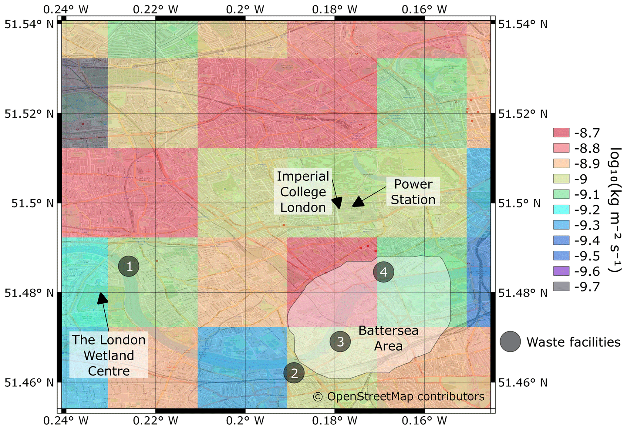
Figure 1Map of the surrounding area of Imperial College London with the UK CH4 1 km2 NAEI estimates overlaid. The locations of large CH4 sources are indicated. The Battersea area is denoted by the white irregular polygon. © OpenStreetMap contributors 2019. Distributed under the Open Data Commons Open Database License (ODbL) v1.0.
There are several large potential sources of CH4 in the vicinity of ICL that may influence the atmospheric CH4 and δ13CH4 measurements. The locations of some of these sources are highlighted in Fig. 1 with the UK NAEI CH4 1 km2 emissions superimposed. There are ∼ 20 small sewage pumping stations and a waste facility (marker 3 in Fig. 1) south of the site in the Battersea area (Fig. 1). The precise locations of these small sewage stations are unknown, but the approximate area is shown in Fig. 1 (Thames Water, personal communication, October 2020). An on-campus natural-gas-fired power station is located in the basement of the electrical and electronic engineering building (∼ 200 m east of the inlet) with the stack emitting at ∼ 52 m a.g.l. (Sparks and Toumi, 2010). Eddy-covariance measurements of CO2 previously conducted from the top of the adjacent building frequently detected emissions from the power station and found a mean CO2 flux of 18.6 µmol m−2 s−1 from the power station (Sparks and Toumi, 2010). This was ∼ 70 % smaller than the UK CO2 NAEI estimate of emissions from the power station at the time. The UK NAEI inventory estimates CH4 emissions from the power station are 3.47×10³ kg CH4 yr−1 (NAEI, 2017; Fig. 1).
2.2 Picarro calibrations and data correction
2.2.1 Measurement set-up
Outside air is drawn into the lab through a Synflex tube by a 30 L min−1 KNF LABOPORT pump. Air is dried to water levels of 0.01 % using a Nafion Perma Pure gas dryer (PD-50-24) in the split sample configuration with a 5 L min−1 diaphragm pump for the counterflow. The Nafion dryer was installed in August 2019. A water correction (Sect. 2.2.4) was applied to the sample air between March 2018 and August 2019 when the air was not dried. A Picarro 16-port manifold is used to switch valves and direct either outside air or standard tank air into the Picarro. A pressure controller between the manifold and the Picarro inlet (PC-100PSIA-D/5P, Alicat Scientific, Inc.) is used to keep the inlet pressure constant at approximately 14 psia (96.5 kPa).
2.2.2 Allan precision
An Allan precision (Allan, 1966) was calculated to measure the noise and drift response of the instrumentation over different averaging times. Two air tanks with ambient CH4 mole fractions and δ13CH4, referred to as the “low” standard (1900 ppb, −48.0 ‰) and “high” standard (2200 ppb, −47.0 ‰), were each measured continuously for 24 h. An averaging time of 4 min has Allan precisions of 0.3 ‰ and 0.2 ‰ for the low and high standard δ13CH4 values (Fig. S1), respectively. This is consistent with previous tests carried out with Picarro G2201-i instruments (Miles et al., 2018; Rella et al., 2015). An averaging time of 20 min reduces the Allan precision to less than 0.1 ‰.
2.2.3 Calibration procedure and measurement uncertainty
Different calibration procedures were tested using one air tank as a working standard to correct for instrument drift and another air tank as a target tank to assess the standard deviation of the measurements. We assumed that the response of the instrument was linear within the observed range (−50 ‰ to −42 ‰, 1900 to 4000 ppb) (Rella et al., 2015) and that the working standard is stable, and we applied a one-point calibration by measuring the working standard once per day for an hour. The “bracketing technique” was used to correct for instrumental drift; i.e. the measurements were calibrated against the time-interpolated value of two adjacent standard measurements. There was an average daily drift of 0.25 ppb for CH4 and 0.7 ‰ for δ13CH4. Both air tanks were calibrated against two primary standards which were prepared at the Max Planck Institute for Biogeochemistry (MPI-BGC). Specific guidelines for calibration procedures of δ13CH4 are not reported in the latest Global Atmospheric Watch programme (20th World Meteorological Organization (WMO)/International Atomic Energy Agency (IAEA) Meeting on Carbon Dioxide, Other Greenhouse Gases and Related Measurement Techniques; WMO, 2020), so each laboratory has to develop a customized calibration routine.
Primary standards had a δ13CH4 uncertainty of 0.20 ‰ (JRAS-M16 scale) and a CH4 uncertainty of 0.25 ppb (WMO CH4 X2004A scale). The working standards had uncertainties of 0.2 ppb for CH4 and 0.18 ‰ for δ13CH4, which are based on the standard deviation of the measurements calibrated against the primary standards. Propagating the error of the primary standard gives a δ13CH4 uncertainty of 0.27 ‰ for our working standard.
We tested calibrations based on the ratio or the offset correction between the measured value of the standard and the assigned calibrated value. Ratio-based calibration adjusts the slope; thus the correction varies with the measured value, whereas offset correction-based calibration adjusts the intercept, and the correction does not vary across the measured value. Some studies recommend calibration of individual isotopologues (Griffith, 2018), while others use δ13CH4 (Rella et al., 2015). The following calibration procedures for δ13CH4 were tested:
-
The 13CH4 and 12CH4 mole fractions were calibrated independently based on the ratio, and then a calibrated δ13CH4 was computed.
-
The 13CH4 and 12CH4 mole fractions were calibrated independently based on the offset correction, and then a calibrated δ13CH4 was computed.
-
The δ13CH4 values were calibrated directly based on the ratio.
-
The δ13CH4 values were calibrated directly based on the offset correction.
We applied the different calibration procedures to 20 min averaged measurements of the target from May 2019 to November 2019. All the calibration procedures performed comparably and reduced the standard deviation of the target tank δ13CH4 values from 1.1 ‰ to 0.2 ‰. We chose to apply a one-point calibration based on the ratio between the measured standard value and the assigned δ13CH4 value, which is the default calibration procedure used by GCWerks software. Whilst a two-point calibration yields a smaller uncertainty, it could not be performed as the δ13CH4 values of the two standard tanks (in which one is used as the target tank) are too similar, differing by 0.3 ‰, and we assume the working standard is stable over time. Rella et al. (2015) also applied calibration constants on the δ13CH4 values rather than on the 13CH4 values. The total CH4 mole fraction was calculated using calibrated 12CH4 and δ13CH4 values, in which 12CH4 was also calibrated using a one-point calibration based on the ratio of the measured and assigned values. We regard the standard deviation of calibrated CH4 mole fractions and δ13CH4 in the target tank to be the best indicator of our measurement uncertainty, at 0.28 ppb and 0.2 ‰ for 20 min averages after May 2019 and 1.8 ppb and 0.6 ‰ before May 2019. The mean of the standard deviations of each standard tank is 0.18 ppb and 0.5 ‰ before May 2019 and 0.16 ppb and 0.4 ‰ after May 2019 for CH4 and δ13CH4, respectively. The larger uncertainty before May 2019 is likely related to unexplained larger variations in the measurements of one of the reference tanks.
A correlation between atmospheric pressure and δ13CH4 is seen in the raw measurements, which has been observed for CO in other Picarro analysers (Yver Kwok et al., 2015). The daily working tank calibrations removed the effect of atmospheric pressure variations over more than 1 d. For some days when atmospheric pressure changed rapidly within one day, artefacts appeared in δ13CH4. The δ13CH4 measurements were inspected for periods of high variability in atmospheric pressure and was manually flagged to remove these artefacts.
Here, measurements at ICL were compared to the δ13CH4 observations at the Mace Head Observatory carried out by the Institute of Arctic and Alpine Research (INSTAAR) of the University of Colorado. Therefore, we applied a value of +0.28 ‰ to correct for the laboratory offset between INSTAAR and MPI-BGC measurements (Umezawa et al., 2018).
2.2.4 Water correction
A cross interference from water has been observed on the δ13CH4 values during the period March 2018–August 2019 when sample air was not dried. Rella et al. (2015) state the gas stream should be dried to < 0.1 % water vapour content to increase measurement accuracy. Data measured before applying the Nafion dryer were corrected for the water vapour influence. To determine the correction coefficients, the water vapour concentration of a working standard with a δ13CH4 value of −48.5 ‰ was varied using the set-up in Supplement Fig. S2. Two mass flow controllers were used to adjust the flow rates through the bubbler enabling us to calculate the water correction values for water vapour content between 0 % and 2.2 % (Fig. S2). Five measurement cycles (each cycle lasting ∼ 6 h) with δ13CH4 values increasing with water vapour concentration are shown in Fig. S3a. The correction coefficients were determined by applying a least squares regression on the ratio of wet-to-dry δ13CH4 values against the water concentration (Fig. S3b). Using the calibrated working standard δ13CH4 value of −48.5 ‰ as the dry value, we calculated the following equation to correct for the water dependency.
The errors of the linear regression parameters from the water vapour correction experiment were ∼ 10−3 ‰, suggesting there is no additional uncertainty resulting from the water vapour correction.
We did not find any water interference on the CH4 mole fraction measurements,
2.3 Keeling plot analysis
The Keeling plot technique (Keeling, 1961; Pataki et al., 2003) was used to assess isotopic signatures (δs) of local and regional sources by analysing data across three different moving time intervals or “windows” that were 12 h, 3 d, and 7 d in length. We expect that the δs values obtained with the 12 h window emphasize sources local to the measurement site, particularly the local emissions that accumulate in the nocturnal boundary layer. For the 3 and 7 d time windows we used only daytime data between 13:00 and 17:00 UTC (all times are in coordinated universal time) when the planetary boundary layer (PBL) is at its largest to find δs values more representative of sources from the wider area. For all three time windows an orthogonal distance regression was applied to the 20 min averaged data using an automated algorithm, similar to Röckmann et al. (2016). To ensure a coherent pollution event was captured, the δs value from each moving window was retained if the mole fractions varied by more than 150 ppb. The choice of this criterion (i.e. the mole fraction peak strength) was based on simulation experiments using pseudo data (Supplement: Approach for automated Keeling plot analysis).
2.4 Atmospheric simulations
2.4.1 NAME footprints
Simulations of atmospheric CH4 at ICL were performed using the UK Met Office Lagrangian dispersion model NAME with meteorological fields from the UK Met Office's Unified Model (UM). NAME back trajectories were used to calculate “footprints” of surface emission sensitivities. Each grid cell of the footprint describes the impact an emission from that grid cell would have on the mole fraction measured at the receptor site at a certain time (Manning et al., 2011; Rigby et al., 2012).
Three sets of hourly footprints were generated, each with a different horizontal spatial resolution: ∼ 25, ∼ 10, and ∼ 2 km (Table 1). The domain of the 2 km resolution footprints covers the British Isles and a small portion of northern Europe, the domain of the 10 km resolution footprints covers most of Europe, and the domain of the 25 km resolution footprints extends to central northern America (Fig. 2). The 2 and 10 km simulations used a 6 d back-trajectory duration, whereas the 25 km simulations used a 30 d back-trajectory duration. Particle release rates of 2×10⁴ h−1 were used for the 25 and 10 km footprints and 1.5×10⁴ h−1 for the 2 km footprints. Footprints used the Met Office UM UK meteorological fields over the UK and UM global meteorological fields for the rest of the modelling domain. To compare simulations that used footprints with different modelling domains we created nested footprints that used the higher-resolution footprints for the inner domain and the coarser footprints for the outer domain(s) (Table 2).
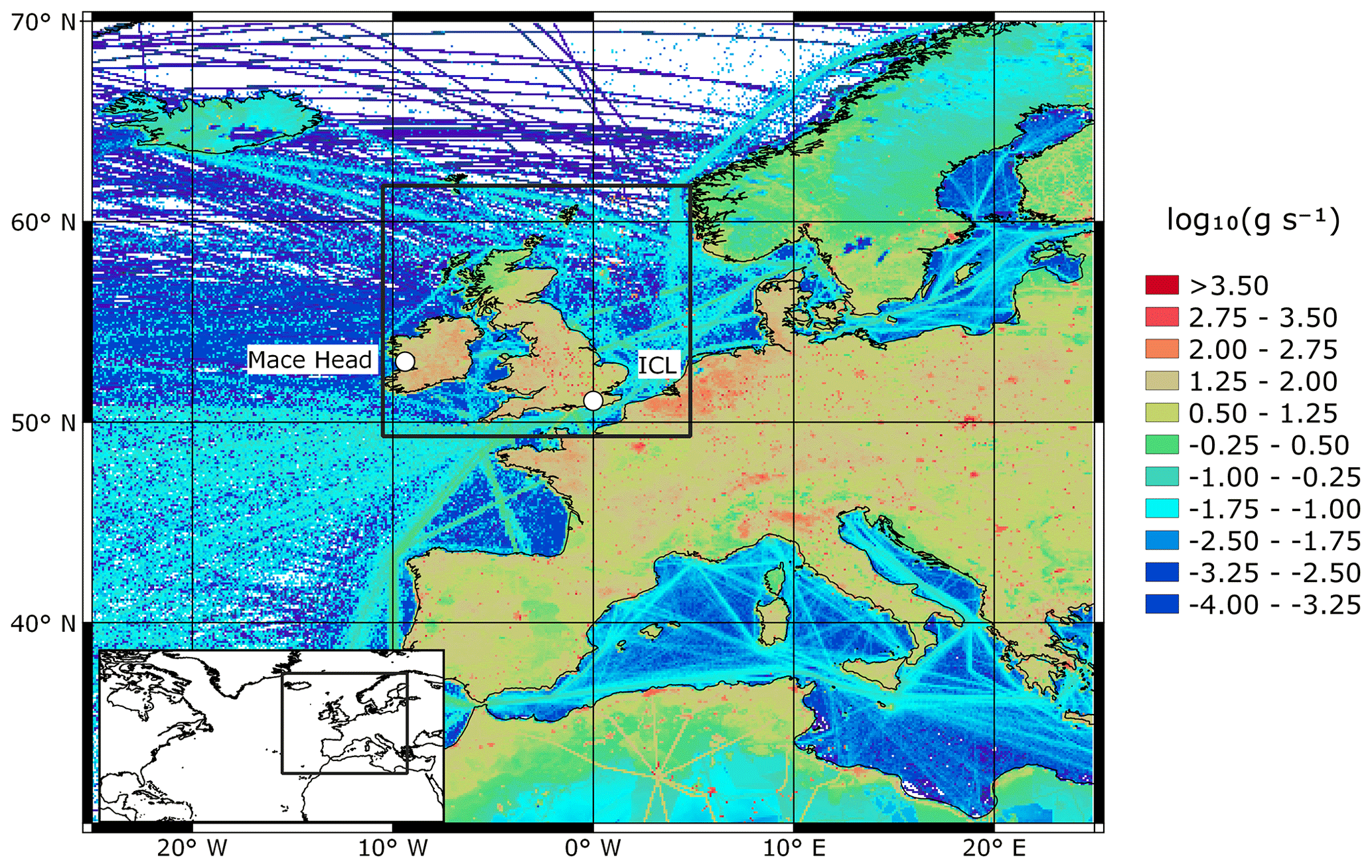
Figure 2The NAME footprint modelling domains. The inset map denotes the area encompassed by the 25 km footprints. The black box denotes the domain of the 10 km footprints, which is shown in the main frame along with the EDGAR v4.3.2 emissions. The black box surrounding the British Isles denotes the 2 km footprint domain.
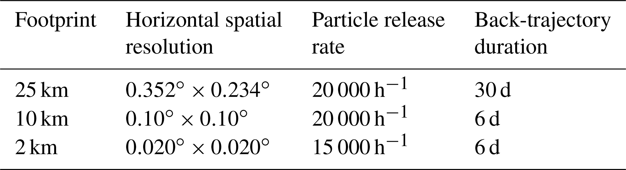
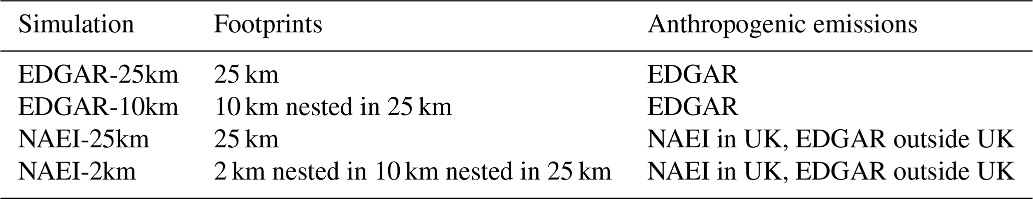
Table 2Summary of atmospheric CH4 simulations. WetCHARTs and GFED4 were used for wetland and biomass burning emissions in all simulations.
Footprints were combined with gridded emissions (Sect. 2.4.2) to simulate CH4 mole fractions above the background mole fractions outside the footprint domain (i.e. excess CH4 mole fractions). To compare the simulated excess CH4 mole fractions to the measurements at ICL, we subtract daily background CH4 mole fractions from the Mace Head Observatory (Arnold et al., 2018; Manning et al., 2021) from the 20 min averaged measurements at ICL. Daily background CH4 mole fractions representative of mid-latitude northern hemispheric concentrations are calculated following the methodology presented in Arnold et al. (2018) and Manning et al. (2021).
Simulated atmospheric δ13CH4 (δair) values were calculated from a weighted average of the isotopic signatures of individual source sector components of excess CH4 using the NAME simulations and the background δ13CH4 (δbg) at Mace Head following
where Ci and δi are the excess CH4 and isotopic signatures of the individual source sectors, and Cbg and δbg are the background CH4 mole fraction and δ13CH4.
Background δ13CH4 values were calculated using measurements at Mace Head by following the method outlined in Manning et al. (2011). Footprints at Mace Head are used to assess which measurements were not influenced by significant emissions and are suitable as background measurements. We fit a curve of multiple harmonics (e.g. Jones et al., 2015) to the background measurements at Mace Head from January 2018 to May 2020. We extrapolate to October 2020 by fitting a linear trend to the data and assuming the same seasonal cycle to obtain a time series of daily δ13CH4 values that match the period of ICL observations.
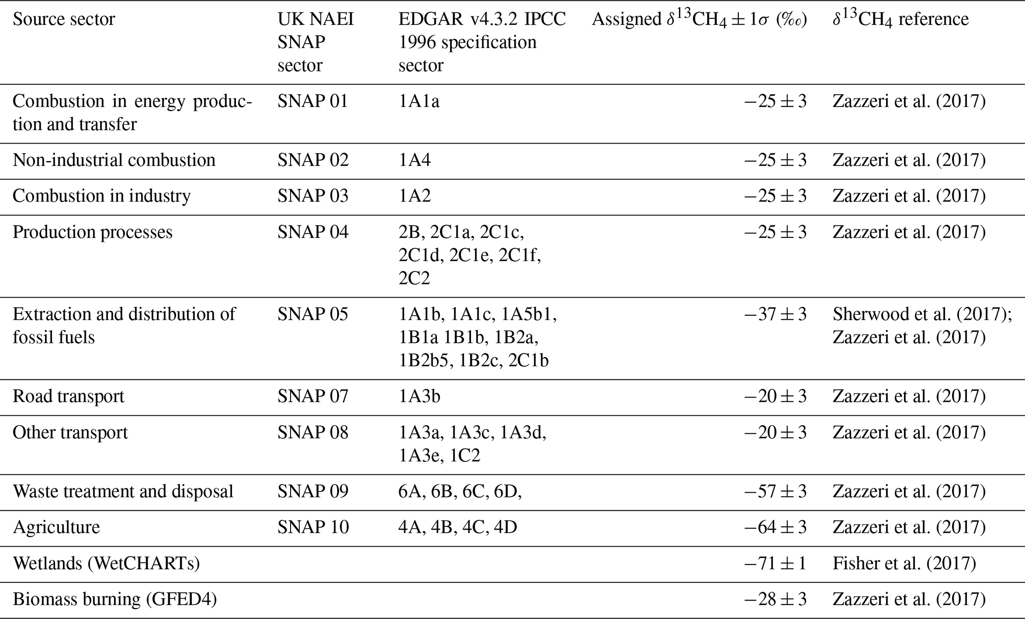
Table 3 lists the isotopic signature assigned to each source sector in the UK NAEI and EDGAR inventories, based on the UK-specific isotopic source signatures from Zazzeri et al. (2017). For anthropogenic source sectors that did not have a UK-specific isotopic source signature (petroleum refining, 1A1b, and oil, 1B2a, in EDGAR), global values from Sherwood et al. (2017) were used. Some source sectors are composed of multiple sources with different isotopic source signatures; for example the waste sector includes landfill sites and waste water treatment facilities. In this case the weighted average of the different sources, based on the UK emissions reported to the UNFCCC (https://di.unfccc.int/comparison_by_category, last access: November 2020), was used to calculate the isotopic source signature of that source sector.
Table 3The correspondence and allocation of methane sources between NAEI and EDGAR along with the assigned δ13CH4 value for each source sector.
2.4.2 Emissions data
We used two sources of anthropogenic CH4 emissions data. The first is the Emissions Database for Global Atmospheric Research (EDGAR) v4.3.2 for the year 2012 with spatial resolution. The second is the UK National Atmospheric Emissions Inventory (NAEI) for 2017 with 1 km × 1 km spatial resolution, where we added point source emissions to the mapped emissions (which omit point sources) using the locations of the point sources. The NAEI is only available for the UK, so for simulations using the NAEI we created a hybrid emissions map with NAEI emissions for the UK and EDGAR emissions for outside the UK. Both emissions inventories have a yearly time resolution, but neither provide gridded numerical uncertainties.
The two inventories use different sectoral definitions. The UK NAEI uses Corinair Selected Nomenclature for sources of Air Pollution (SNAP) in which sources are allocated to 1 of 11 categories, whereas EDGAR follows the 1996 IPCC source sector specification in which sources are allocated to one of seven categories and then further subdivided. For example, emissions from landfills in EDGAR form a subset of waste sector emissions (category number six) and are specified as category 6A (Table 3), whereas in NAEI all waste emissions are aggregated under SNAP 09 (Table 3). Table 3 shows how we aligned the sources between inventories.
For wetland emissions we used the mean of the 2015 extended ensemble WetCHARTs inventory (Bloom et al., 2017). The extended ensemble consists of 18 models with a spatial resolution of and a monthly temporal resolution. For biomass burning emissions we used the Global Fire Emissions Database v4 (GFED4; van der Werf et al., 2017) for 2016 at resolution and a monthly temporal resolution. To avoid double counting we excluded agricultural waste burning emissions from GFED4.
The four sets of anthropogenic emissions for the London area are shown in Fig. 3a–d. The UK NAEI emissions are approximately 2.5 times smaller than the EDGAR emissions for the London area (Table 4; Fig. 3e) but 8 % smaller than the EDGAR emissions across the UK (Fig. 3f). The 2 km NAEI and 10 km EDGAR show high emissions from individual grid cells that are smoothed out in the coarser 25 km EDGAR grid (Fig. 3a) and 25 km NAEI grid (Fig. 3c). Subtracting the 25 km NAEI emissions from the 25 km EDGAR emissions (Fig. 3e–f) indicates that the largest differences between inventories were in cities: London, Birmingham, and the Leeds–Sheffield area, which have higher emissions in the EDGAR inventory. This shows that emissions in urban areas are particularly uncertain and in need of additional constraints.
Table 4EDGAR and NAEI emissions for the UK and London. δ13CH4 is the weighted average of different emission sectors using isotopic source signatures in Table 3.

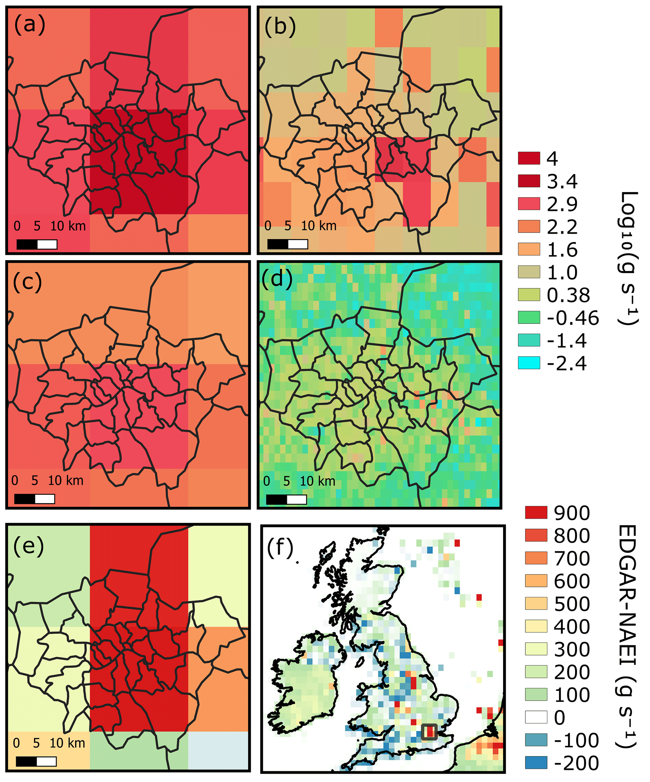
Figure 3London CH4 emissions from (a) EDGAR v4.3.2 (2012) scaled at 0.352∘ × 0.234∘, (b) EDGAR scaled at 0.10∘ × 0.10∘, (c) UK NAEI (2017) scaled at 0.352∘ × 0.234∘, and (d) UK NAEI scaled at 0.02∘ × 0.02∘. The NAEI scaled at 0.352∘ × 0.234∘ subtracted from the EDGAR emissions (in g s−1) for London is shown in (e) and for the UK in (f). The London region in relation to the UK is shown by the black box in (f).
We considered four combinations of footprints coupled with anthropogenic emissions data: (i) the 25 km footprints combined with the EDGAR emissions (EDGAR-25km); (ii) the 10 km footprints nested in the 25 km footprints combined with the EDGAR emissions (EDGAR-10km); (iii) the 25 km footprints combined with the UK NAEI emissions for the UK and the EDGAR emissions for the rest of the domain (NAEI-25km); and (iv) the 2 km footprints nested in the 10 and 25 km footprints combined with the UK NAEI emissions for the UK and EDGAR for the rest of the domain (NAEI-2km). These are summarized in Table 2.
3.1 Measurements
The 20 min averaged CH4 mole fractions from March 2018 to October 2020 along with the Mace Head background values are shown in Fig. 4a. Mole fractions ranged from 1895 to 3924 ppb in the ICL measurements with a mean value of 2083±145 (1σ) ppb. ICL mole fractions measured during the afternoon (13:00–17:00) were lower on mean, 2028±73 (1σ) ppb, and had a lower maximum value, 2477 ppb, showing that higher concentrations are observed during the night-time from the build-up of emissions in the nocturnal boundary layer. The Mace Head background mole fractions ranged from 1907 to 1973 ppb and had a mean value of 1939±13 (1σ) ppb. During the first UK COVID-19 lockdown period (23 March 2020–15 June 2020), we observe more days with higher CH4 mole fractions compared to the preceding months (Fig. 4a). This did not result in a difference between the average mole fractions before and during the UK COVID-19 lockdown period (Fig. 5a).

Figure 4The 20 min averaged measured (a) mole fractions and (b) δ13CH4 values at ICL, along with the daily Mace Head background values from March 2018 to October 2020. Afternoon (13:00–17:00) data are shown in black. The period of the first UK national COVID-19 lockdown is denoted by the pink region. The dashed grey line denotes when the standard and target tanks were changed.
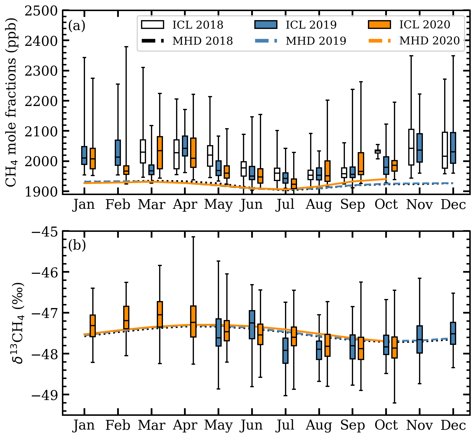
Figure 5Seasonal cycles of detrended 20 min measurements of (a) mole fractions and (b) δ13CH4 at ICL (box plots) and Mace Head (lines) in which values deviate around 1 March 2018 (tref) for mole fractions and around 1 May 2019 (tref) for δ13CH4.
The δ13CH4 measurements at ICL are shown in Fig. 4b along with the calculated Mace Head background δ13CH4 values. The mean δ13CH4 at ICL for this period is ‰ with values ranging from −52.4 ‰ to −42.3 ‰. The afternoon δ13CH4 mean was nearly the same, ‰. Mace Head background δ13CH4 averaged ‰ and ranged from −48.0 ‰ to −47.4 ‰. Observed δ13CH4 at ICL was generally higher than δ13CH4 at Mace Head during 2018, but excursions both higher and lower than the background are seen during 2019–2020. We see a mean 0.05 ‰ increase in δ13CH4 at ICL during the UK COVID-19 lockdown period, but this could be due to seasonal changes rather than anthropogenic influences.
The ICL mole fractions were detrended by fitting a linear polynomial to Mace Head data to find the trend between 2018 and 2020 with the mole fraction on 1 March 2018 set as the reference point, tref. Detrended mole fractions were binned by month to evaluate seasonal variations (Fig. 5a). A seasonal cycle is observed with a CH4 minimum occurring in July for both ICL and Mace Head measurements. Smaller interquartile ranges and smaller maximum values in the ICL mole fractions are observed in the summer months. Diurnal cycles are observed in the detrended ICL mole fractions with daily minimums between 13:00 and 15:00 (Fig. 6a) with generally smaller mole fractions between April and September. Differences in the diurnal cycles throughout the week vary depending on the time of year. The average nocturnal build-up of CH4 is significantly larger on Monday and Tuesday in the July–August–September (JAS) averaged mole fractions compared to the rest of the week (Fig. 6a), whereas the October–November–December (OND) averaged mole fractions have relatively similar levels of CH4 nocturnal build-up throughout the week.

Figure 6Weekly detrended 20 min averages of (a) mole fractions and (b) δ13CH4 at ICL (values normalized to 1 March 2018 and 1 May 2019, tref, respectively). Measurements are grouped by season of year and binned by hour of day and day of week. The 1σ range is included on both panels.
In our analysis we focus on δ13CH4 measurements from May 2019 onwards as large unexplained variations in one of the reference tanks before May 2019 result in larger δ13CH4 uncertainties (Sect. 2.2.3). Afternoon measurements of δ13CH4 at ICL were detrended by fitting a linear polynomial to Mace Head background δ13CH4 from 2018 to 2020 with δ13CH4 on 1 May 2019 set as the reference point, tref (Fig. 5b). ICL median δ13CH4 between January and March were generally higher than the Mace Head background and generally lower from July through to September. The δ13CH4 ICL measurements averaged into hourly intervals tend to exhibit lower δ13CH4 during the afternoon but no well-defined diurnal or weekly cycle (Fig. 6b).
3.1.1 Keeling plot analyses
Three moving time windows of lengths 12 h, 3 d, and 7 d were used in the automated Keeling plot algorithm to find δs values between May 2019 and October 2020 (Figs. 7–8). The calculated δs values may correspond to an individual source sector (Table 3), but they can reflect mixtures of different sources influencing the measured air in each time window, in which the δs is a weighted average of the different sources. Isotopic source values lower than −47 ‰ suggest the sources are primarily biogenic (waste and/or agriculture), and δs values higher than −47 ‰ suggest the sources are primarily from gas leaks from the CH4 gas distribution network (i.e. natural gas leaks), in which −47 ‰ is the midpoint between the waste and the natural gas CH4 isotopic signatures (Table 3). Isotopic source values are sorted into 5 ‰ bins; therefore we use −45 ‰ to distinguish between primarily biogenic and primarily natural gas CH4 sources.
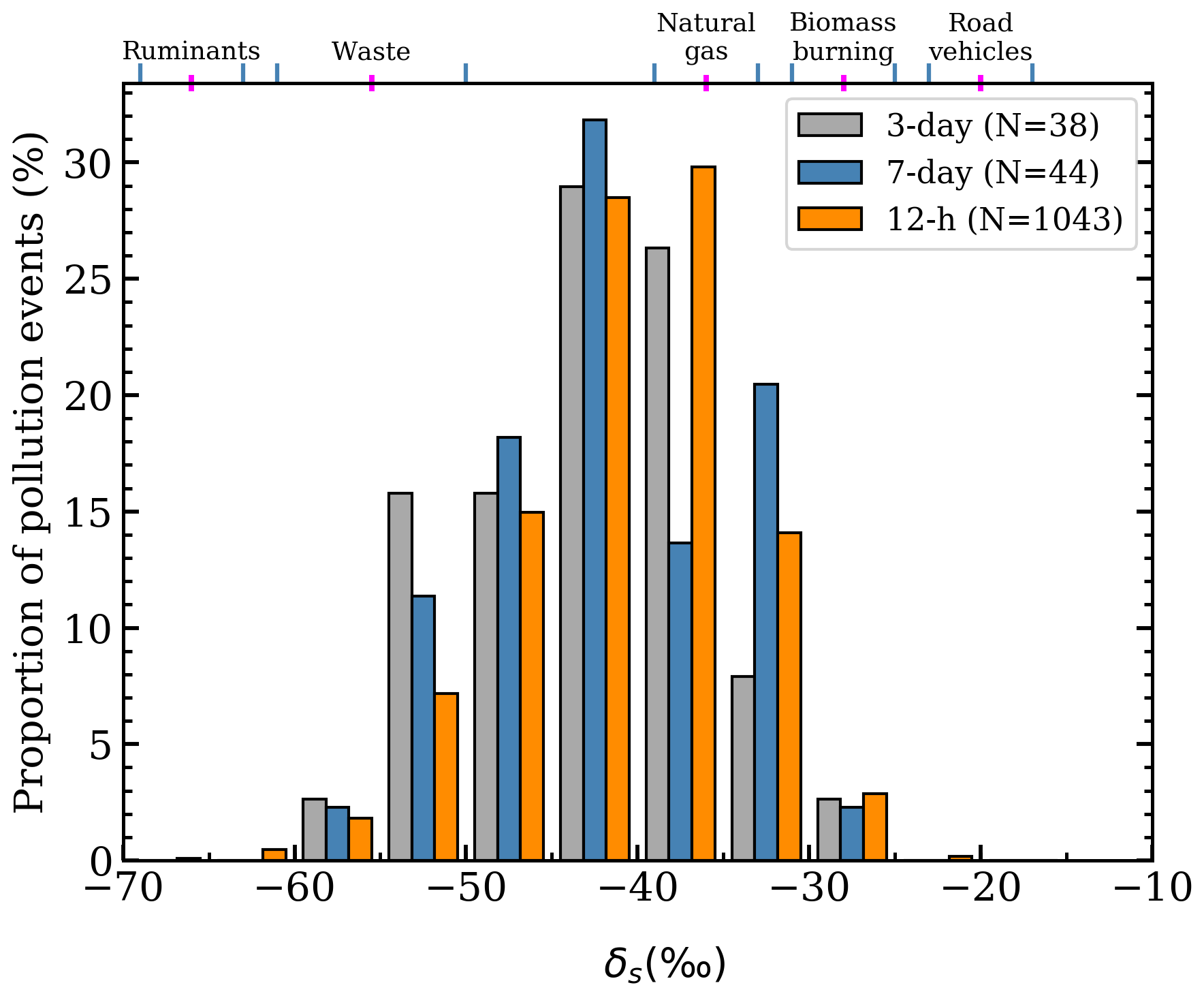
Figure 7The distributions of the isotopic source values from Keeling plot analysis. The ranges of different UK isotopic signatures from Zazzeri et al. (2017) are shown at the top for reference.
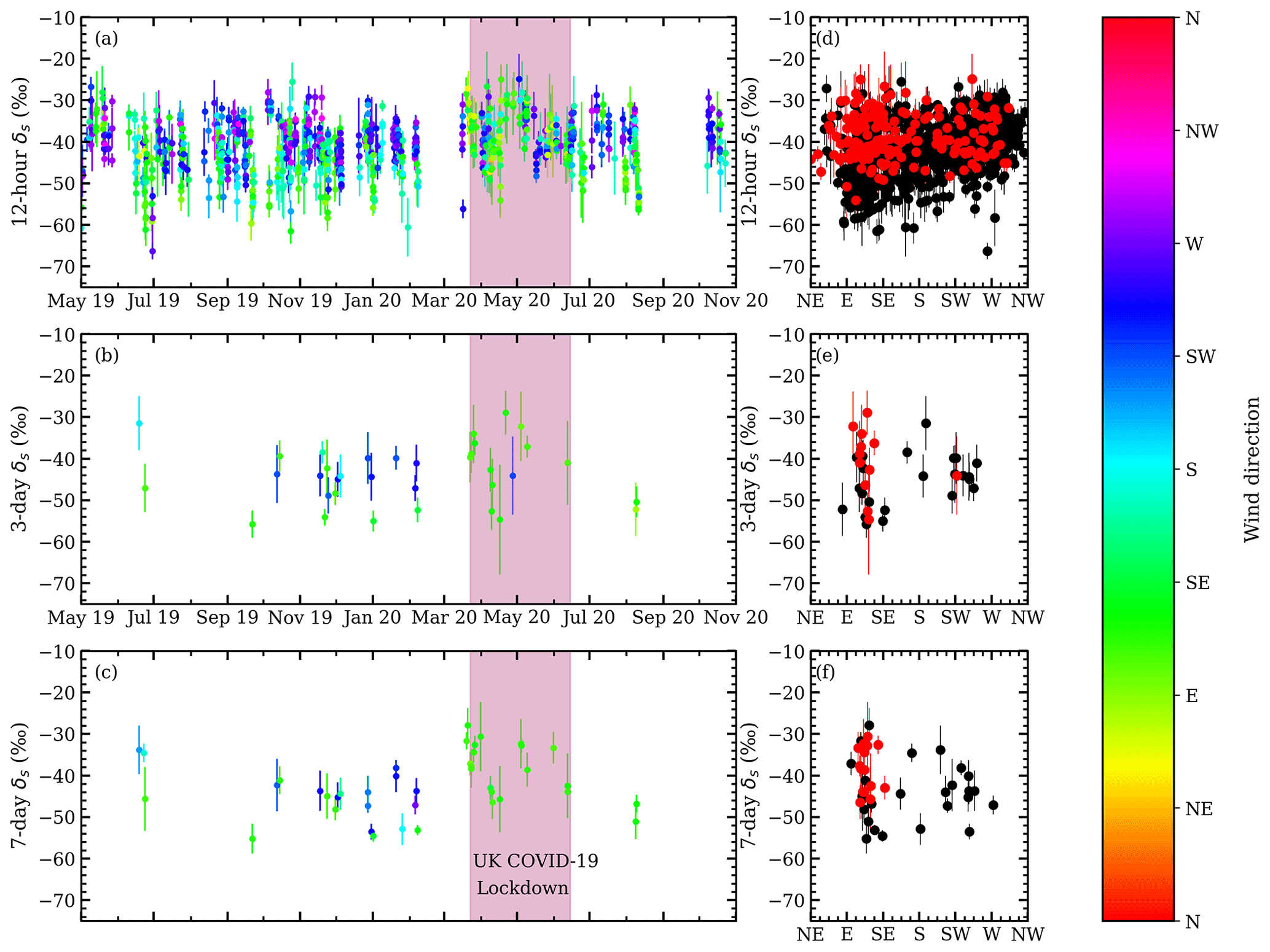
Figure 8Time-series of isotopic source values for (a) 12 h, (b) 3 d, and (c) 7 d windows. The marker colour denotes the mean wind direction from the start of the window to the peak of the pollution event. Black markers indicate times when wind direction data were not available. The UK COVID-19 lockdown period is shown in pink. Isotopic source values and wind direction comparisons for each of the moving windows are shown in panels (d–f). Red markers denote the period of the first UK COVID-19 lockdown.
The 12 h moving windows, using measurements from all hours, returned 1046 δs values, of which 24.5 % were ‰. Most of the 12 h pollution events occurred during the nocturnal CH4 build-up, and the large number of δs values > −45 ‰ suggests natural gas sources are primarily driving the nocturnal CH4 build-up around ICL. Natural gas leaks are expected to have a signature of ‰ in London (Zazzeri et al., 2017). Uncertainties in δs were 2.8 ‰ in the 12 h windows.
The 3 and 7 d windows using 13:00–17:00 measurements returned 41 and 47 δs values, respectively, and have higher proportions of biogenic influences. In the 3 d windows, 26.3 % of δs values were ‰, and in the 7 d windows, 20.5 % of δs values were ‰. Still a majority of pollution events had δs values > −45 ‰, showing that natural gas leaks are the main source of CH4 pollution at ICL sampled in the afternoon and arising from larger-scale regional influences, in addition to the presumably more local sources sampled in the night. Uncertainties in δs were 4.4 ‰ in the 3 and 7 d windows.
The δs values between −30 ‰ and −25 ‰ may arise from a mixture of vehicular and natural gas CH4, but they have mole fraction peak strengths (Sect. 2.3) smaller than 200 ppb, and they comprise less than 5 % of the isotopic source values, indicating CH4 emissions from the nearby roads and power station are small.
We looked for a relationship between wind direction and δs values (Fig. 8), but we do not find any consistent patterns, which reflects the collocation and heterogeneity of sources in London. Some events with low isotopic signatures and wind direction in the southerly or southwesterly direction may be influenced by the sewage or landfill sites south or southwest of ICL (Fig. 1). The δs values observed during the UK COVID lockdown period were ∼ 2 ‰ higher in the 12 h windows and ∼ 5 ‰ higher in the 3 and 7 d windows compared to the months before and after the lockdown. However, during the UK COVID lockdown period there was an unusual predominance of easterly winds.
3.2 Simulations of methane
3.2.1 Simulated CH4 mole fractions
Afternoon simulations of CH4 mole fractions are compared with the afternoon observations at ICL in Fig. 9 for 2020 (Figs. S6, S7 for 2018 and 2019) and in Fig. 10 for all years. As previously highlighted, afternoon mole fractions are less sensitive to local emissions and provide a more accurate representation of regional-scale CH4 sources and mole fraction variations. Afternoon weather conditions tend to be represented better in models as errors in the modelled planetary boundary layer are considered smaller during the afternoon (Brophy et al., 2019; Jeong et al., 2013). Simulated CH4 using UK NAEI tends to be lower than the ICL measurements. Higher simulated mole fractions with EDGAR are expected as emissions in EDGAR are 2.5 times larger than the NAEI emissions for the London area (Table 4).
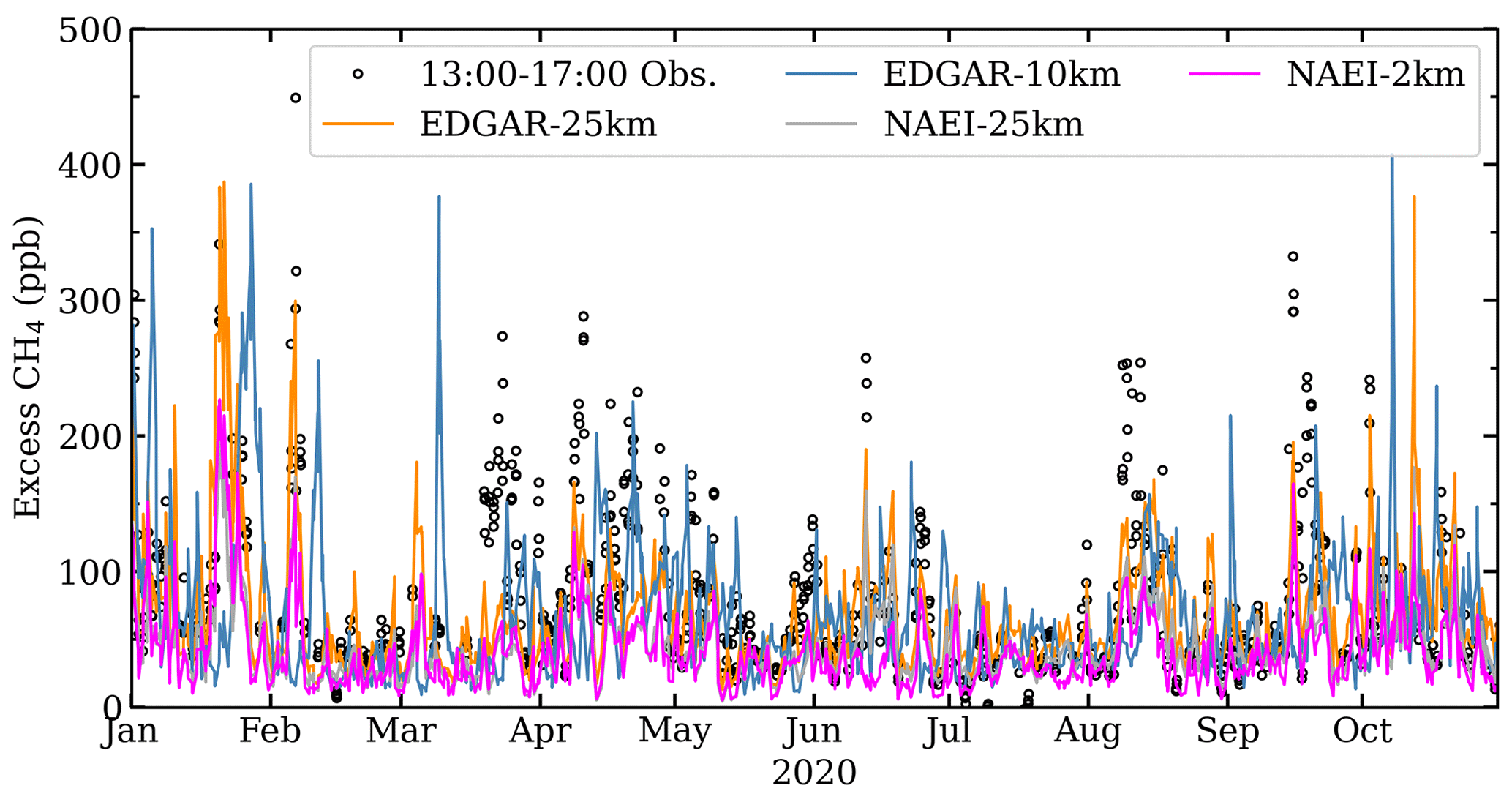
Figure 9Excess simulated and observed 13:00–17:00 mole fractions for 2020 in which the Mace Head background has been subtracted from the ICL measurements.
The slope of the linear regressions (Fig. 10a–d), the RMSE, and the median simulation–observation differences (Fig. 10e–h) are used to compare the simulations with the observations. There are small differences between the slope and intercept values obtained by an ordinary least squares and an orthogonal distance regression.
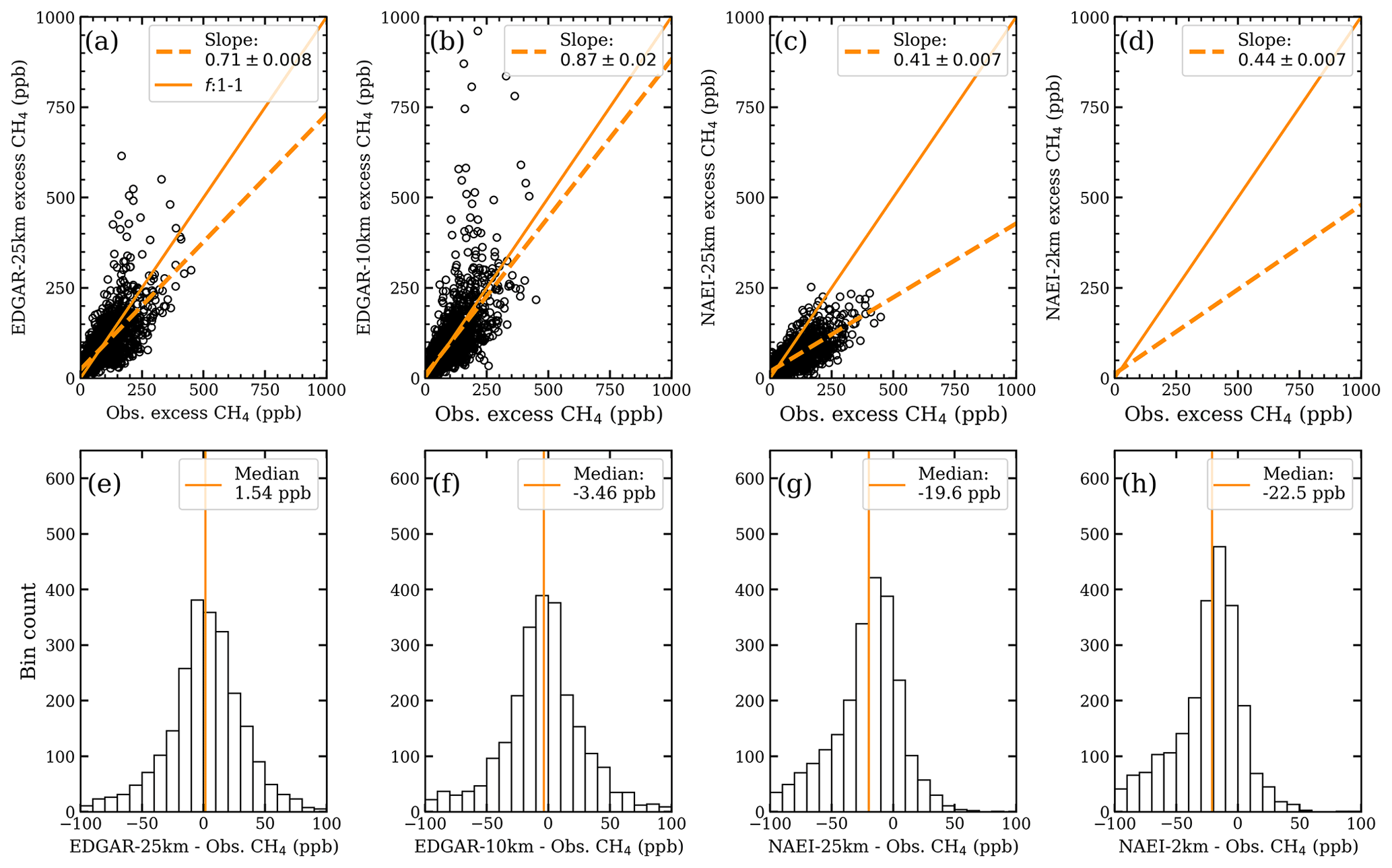
Figure 10Simulation–observation comparisons of excess mole fractions using linear regressions (top row) and distributions of the simulation–observation differences (bottom row) for (a, e) EDGAR-25km, (b, f) EDGAR-10km, (c, g) NAEI-25km, and (d, h) NAEI-2km from March 2018 to October 2020.
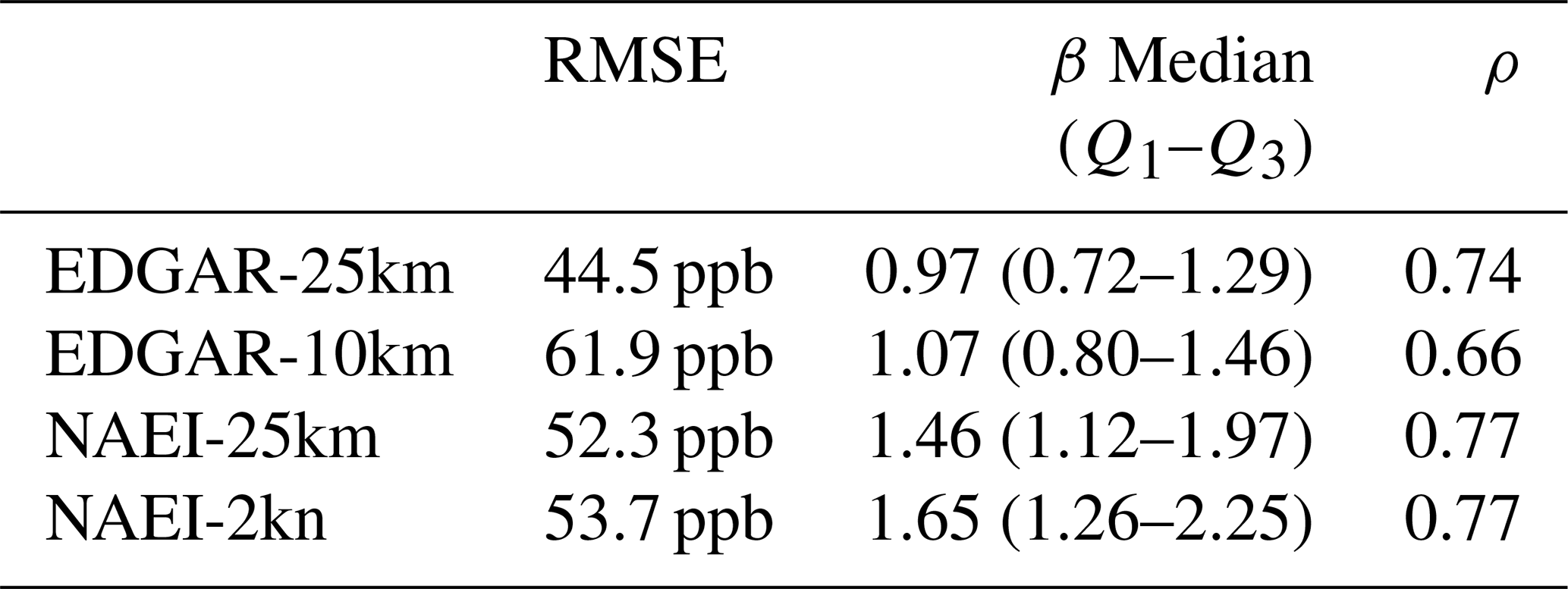
Though EDGAR-10km comparisons (Fig. 10b) have slopes closest to 1, the EDGAR-10km comparisons also have the largest RMSE (61.9 ppb; Table 5), whereas the other simulation–measurement RMSEs are between 44.5 ppb (EDGAR-25km; Table 5) and 53.7 ppb (NAEI-2km; Table 5).
Table 5Simulation–observation 13:00–17:00 RMSE values, scaling factors, and correlation coefficients.
Distributions of simulation–observations (Fig. 10e–h) show 13:00–17:00 EDGAR data have medians closer to zero than NAEI data. EDGAR-10km has a median simulation–measurement difference of 0.93 ppb. The NAEI-25km and NAEI-2km simulation–measurement distributions have afternoon median values of −19.6 and −22.5 ppb, respectively (Fig. 10g–h).
Scaling factors, β, based on the simulation–observation median differences, are calculated by adjusting the simulated values so that they equal the corresponding excess CH4 observation,
where Cobs is the Mace Head background mole fractions subtracted from the ICL measurements. Background mole fractions exert a significant leverage on the values of β. We account for this by varying each daily background mole fraction value by randomly sampling from a Gaussian distribution centred on the daily background value and using the daily standard deviation to vary the mole fraction background and calculate the β values 150 times.
The median β scaling factors are similar in the 13:00–17:00 data with EDGAR simulations having scaling factors closer to 1 (Table 5), suggesting a strong correspondence between the EDGAR emissions and the observations. On average, 13:00–17:00 NAEI-2km simulations need to be scaled by 1.61 and NAEI-25km by 1.42. NAEI simulations have larger interquartile ranges than the EDGAR simulations, suggesting a higher variability in the NAEI simulated mole fractions.
Increasing the spatial resolution in the simulated mole fractions had a small effect in comparison to the differences between using NAEI and EDGAR emissions for the UK. Our conservative gridding approach (Sect. 2.4.2) ensures emissions across a region will be the same for all spatial resolutions. Differences will arise as a result of the width of the different back-trajectory plumes and the emission grid cells they intersect.
3.2.2 Simulations of δ13CH4
Simulated δ13CH4 values are consistently 13C-depleted relative to the background in all simulations (Figs. 11, S8), which contrasts with the observations that show δ13CH4 excursions both above and below the background (Fig. 11). The simulated range in δ13CH4 in NAEI-25km and NAEI-2km is only 0.2 ‰, which reflects the strong similarity between the mean isotopic source signature for London of −47.7 ‰ in NAEI (Table 4) and the background δ13CH4 (−48.0 ‰ to −47.4 ‰). EDGAR-25km and EDGAR-10km also underestimated the variation in δ13CH4 as isotopically heavy pollution events were missing, even though the isotopically light spikes are often exaggerated in EDGAR-10km, as was found for the mole fractions. The mean isotopic source signature for London is −53.7 ‰ in EDGAR (Table 4) due to a large proportion of emissions from waste (93 %) and a small proportion of natural gas (3 %). The proportion of emissions from natural gas is higher in NAEI (41 %), but the mean isotopic source signatures for London in both NAEI and EDGAR are much lower than the median of the isotopic source signatures calculated in the Keeling plot analysis (−41.6 ‰; Fig. 7)
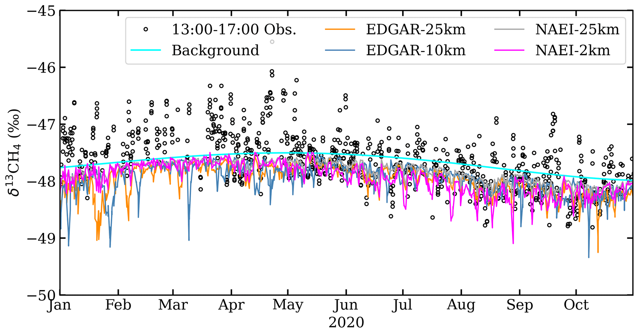
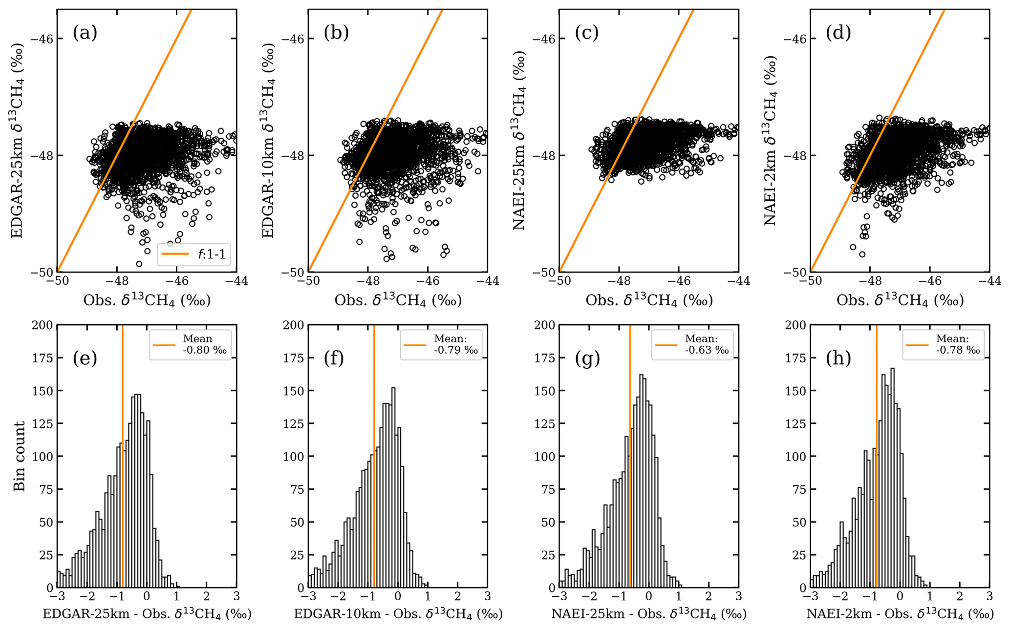
Figure 12Simulation–observation comparisons of δ13CH4 using point-by-point comparisons (top row) and distributions of the simulation–measurement differences (bottom row) for (a, e) EDGAR-25km, (b, f) EDGAR-10km, (c, g) NAEI-25km, and (d, h) NAEI-2km.
Simulation–observation comparisons in Fig. 12a–d do not show any correlation between the measurements and the simulations. The simulation–observation difference distributions (Fig. 12e–h) are all negatively skewed and have mean differences ranging from −0.63 ‰ in the NAEI-2km data to −0.80 ‰ in the EDGAR-25km simulations. This indicates the source apportionments in the NAEI and EDGAR inventories have fossil fractions that are too low, and their sources may be distributed too homogenously.
To test whether the underestimates in excess CH4 mole fractions and in δ13CH4 in the NAEI simulations could be explained solely by underestimated emissions from natural gas leaks, we recalculate δ13CH4 in NAEI-25km and NAEI-2km by assuming all the missing simulated CH4 is natural gas CH4. Scaling factors for the simulated natural gas mole fractions (Sect. 3.2.3), calculated from the overall CH4 scaling factors (Table 5), are 3.7 for NAEI-25km and 4.1 for NAEI-2km. The recalculated δ13CH4 shows much smaller excursions below background δ13CH4 and now some excursions above background δ13CH4 (Fig. 13), particularly in NAEI-2km in which the correlation between observed and simulated δ13CH4 increased from 0.37 to 0.56. However, it appears that the recalculated δ13CH4 reflects a rather homogeneous fossil fraction in excess CH4 with an isotopic signature near to background δ13CH4, which therefore produces very small variations in δ13CH4 in contrast to the observations. This indicates that the locations of natural gas and waste emissions in London are more spatially distinct than in the NAEI inventory.
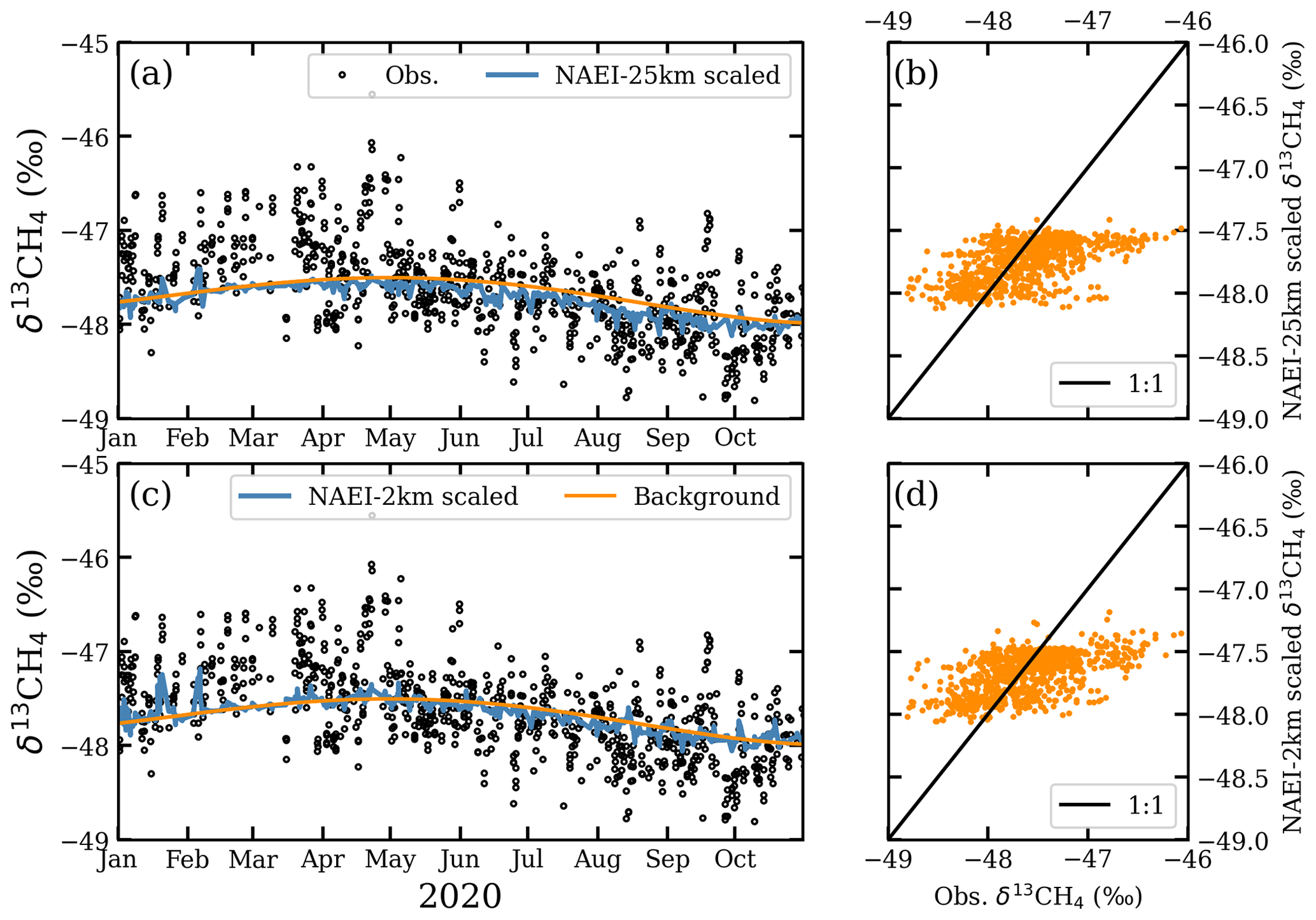
Figure 13Time series comparison of simulated (a) NAEI-25km and (c) NAEI-2km δ13CH4 recalculated by scaling the simulated natural gas mole fractions, along with observations for afternoon hours. Simulation–observation comparisons of δ13CH4 using linear regressions for (b) NAEI-25km and (d) NAEI-2km for 2020 afternoon hours.
3.2.3 Sectoral source apportionment in the simulations
The mean source apportionments at ICL for each set of simulations are given in Table 6. In all four sets of simulations, CH4 from the waste sector dominated at ICL, accounting for between 30.0 % (NAEI-2km) and 71.1 % (EDGAR-25km) of added CH4 (Table 6). Whilst waste CH4 at ICL was more than 3 times larger than any other source sector in EDGAR-25km and EDGAR-10km, waste CH4 was lower and more comparable to natural gas CH4 in NAEI-25km and NAEI-2km. Natural gas CH4 at ICL formed the third largest source in the NAEI-25km (20.4 %) and second largest in the NAEI-2km (28.3 %), but it was significantly smaller in EDGAR-25km (6.2 %) and EDGAR-10km (8.1 %). Agricultural sources at ICL accounted for the second largest source in EDGAR-25km (13.8 %), EDGAR-10km (18.8 %), and NAEI-25km (22.2 %).
Table 6Mean simulated source apportionment for excess CH4 at Imperial College London and in the CH4 emissions for London.
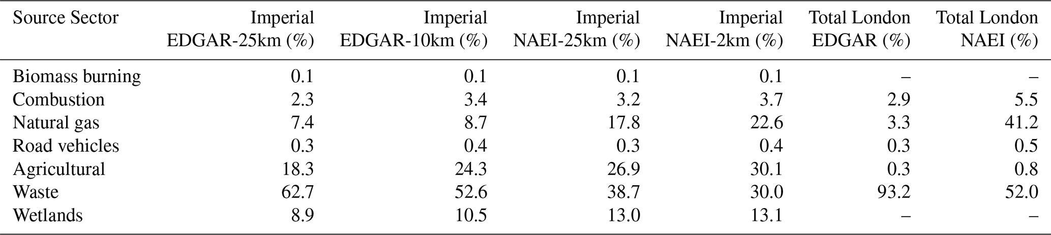
Higher-resolution simulations decreased the proportion of waste sources and increased the proportion of natural gas CH4 sources. The distribution of emissions in lower-resolution simulations is likely to unrealistically smooth the point source emissions from landfills across the London area, increasing the probability of the back trajectories interacting with emissions from these grid cells. For example, NAEI-2km waste emissions are located towards the outskirts of London (Fig. S9d), but NAEI-25km waste emissions are uniformly distributed across London (Fig. S9c). Similarly, natural gas emissions are located near the centre of London (Fig. S10d) but not uniformly distributed in the coarser-resolution emissions due to the absence of natural gas emissions on the outskirts/outside of London (Fig. S10c).
Simulated CH4 from biomass burning sources (GFED4) were negligible (< 0.2 %; Table 6) in comparison to the contributions from other sources. However, CH4 from wetlands formed a more significant proportion of added CH4 (6.0 %–9.8 %; Table 6) with higher contributions during the summer. A pollution event on 16 August 2019 that had a low isotopic source signature (Sect. 3.1.1) coincided with an 80 ppb simulated wetland mole fraction on the same day.
Continuous measurements of CH4 mole fractions and δ13CH4 in central London show, through Keeling plot analyses, a range of different CH4 sources exist in London. Most isotopic source values are > −45 ‰, indicating a high fossil fraction of added CH4 for central London. Comparisons between measurements and the simulated excess mole fractions show a good correspondence between the EDGAR-25km and EDGAR-10km simulations and observations. The NAEI simulations at 2 and 25 km significantly underestimate the observations but retain a good correlation. We calculate the NAEI emissions for London need to be scaled by 1.52 and EDGAR emissions by 0.99 when using the 13:00–17:00 data, which are more representative of the London area and have smaller errors in the modelled boundary layer mole fractions than when night-time data are included. In contrast, we do not observe a correlation between the measured and simulated δ13CH4 values. Unlike the simulated mole fractions, simulated δ13CH4 values are dependent on the source sector spatial distributions in the emission inventories. Simulations of δ13CH4 fail to capture any δ13CH4 excursions above the background as seen in the observations, suggesting the NAEI and EDGAR inventories are underestimating natural gas emissions for the London area.
Under-reported natural gas emissions are reflected in all four δ13CH4 simulations, in which there are few simulated values above the background in contrast to the observations. While the EDGAR-25km and EDGAR-10km mole fraction simulations are most comparable to the observed mole fractions, discrepancies in simulated δ13CH4 show that the apportionment of sources is incorrect in EDGAR. Over 90 % of EDGAR CH4 emissions for London are allocated to the waste sector, which would require leak rates in natural gas infrastructure to be very low, in contrast to observations in other cities with older infrastructure (e.g. McKain et al., 2015). In EDGAR v5.0, not only are CH4 emissions for the UK larger, but these increases have been attributed to waste sector emissions. Potentially there may be even larger discrepancies between urban observations and simulations when using EDGAR v5.0 emissions. The underestimation of mole fractions in the NAEI-25km and NAEI-2km might be accounted for by missing natural gas emissions in the NAEI inventory for London. Scaling the natural gas mole fractions in the NAEI simulations to match the overall excess mole fraction (which increased the natural gas fraction from 22.6 % to 52.1 %) improved the correspondence between the observations and simulated δ13CH4 slightly; however, it appears the spatial allocation of waste and natural gas emissions in the inventory is too homogeneous. Overall, it does not seem possible to improve the model–data comparison for both CH4 mole fractions and δ13CH4 without increasing CH4 emissions from natural gas leaks in the London area in the inventories. More explicit use of δ13CH4 and CH4 data with high-resolution NAME simulations in an inversion framework including consideration of uncertainties in measured, background, and modelled δ13CH4 and CH4 could help to specify the fossil fraction in London more precisely.
Previous ground-based measurement campaigns in London found inventory emissions were underestimated. Helfter et al. (2016) reported mean annual measured emissions of 72±3 t km−2 yr−1, which was more than double the London inventory estimate. Assuming their measured emissions are representative of the greater London area, this is approximately equivalent to 0.11 Tg CH4 yr−1. This is similar to the EDGAR v4.3.2 (2012) estimate of 0.10 Tg CH4 yr−1 for the same London area (Table 4). Simulation–observation comparisons of ICL CH4 mole fractions are in good agreement with the EDGAR emissions estimate, suggesting total London CH4 emissions have not significantly changed since the Helfter et al. (2016) measurement campaign. The median differences between the NAEI simulations and ICL measurements are not as large as those found by Helfter et al. (2016), suggesting some improvement in the NAEI emission estimates for London but with some sources still underestimated.
Isotopic measurements of δ13CH4 by Zazzeri et al. (2017) indicated a predominance of fossil fuel CH4 in central London that was not seen in the NAEI inventory, which estimated 29 % of London CH4 emissions were natural gas CH4 at that time (compared to 41 % in the current inventory). Whether fossil fuel CH4 was underreported or misattributed was an open question as Zazzeri et al. (2017) did not use an atmospheric transport model to generate simulations that could be compared with observed concentrations. Our model–data analysis provides evidence that the NAEI inventory does appear to underestimate natural gas leaks, in agreement with the hypothesis presented in Zazzeri et al. (2017).
The results from these continuous long-term CH4 and δ13CH4 measurements show that they can be used for effective evaluation of CH4 emissions from natural gas and waste sources in urban areas. Measurements from a single site would be significantly enhanced by a larger urban network of CH4 and δ13CH4 measurements encompassing the spatial heterogeneity in different CH4 sources. Measuring from a greater height would also be useful as this would increase the geographical size of the footprint and allow greater mixing of individual sources before measurement.
Measurements of other isotopic tracers, such as deuterium or radiocarbon, or gaseous tracers, such as ethane, would provide additional constraints on the London CH4 source apportionment.
This study presents over 2 years of atmospheric measurements of CH4 mole fractions and δ13CH4 from Imperial College London. Isotopic source values from Keeling plot analysis revealed a predominance of natural gas CH4 with source values higher than −45 ‰ in ∼ 74 %–80 % of the afternoon data. In contrast, simulated sectoral contributions using UK NAEI and EDGAR inventories showed the largest fractions from waste sectors, leading to a simulated underestimation of observed δ13CH4. These results suggest that natural gas leaks in London are under-reported in both inventories, consistent with previous studies in London and some other global cities.
Python 3 scripts are available upon request.
Atmospheric measurement and simulation data are available from the Zenodo repository “Graven Laboratory: Atmospheric methane measurements and simulations” https://doi.org/10.5281/zenodo.6044538 (Graven et al., 2022). Anthropogenic emissions data from EDGAR are available at http://data.europa.eu/89h/jrc-edgar-edgar_v432_ghg_gridmaps (Janssens-Maenhout et al., 2017) and from NAEI at https://naei.beis.gov.uk/data/mapping-archive (NAEI, 2017).
The supplement related to this article is available online at: https://doi.org/10.5194/acp-22-3595-2022-supplement.
Simulations of CH4 were produced in Python by ES. ES ran the NAME transport model under the guidance of AJM and HG for the 10 and 2 km footprints. AJM provided the 25 km footprints. GZ provided the measurement data and wrote Sect. 2.2. Mole fraction background data from Mace Head were provided by AJM and isotopic values by SEM. HG was the main scientific supervisor and provided guidance on the presentation of results. ES was responsible for the development of the paper, which forms part of his PhD. All authors provided feedback on the manuscript.
The contact author has declared that neither they nor their co-authors have any competing interests.
Publisher’s note: Copernicus Publications remains neutral with regard to jurisdictional claims in published maps and institutional affiliations.
This project was funded by the European Research Council (ERC) under the European Union's Horizon 2020 research and innovation programme (grant agreement 679103), the Grantham Institute – Climate Change and the Environment Science and Solutions for a Changing Planet DTP (NE/L002515/1), the UK Natural Environment Research Council (NERC grant NE/S005277/1), and the National Physical Laboratory (NPL, UK). The authors thank the UK Department of Finance for permission to use Northern Ireland UK NAEI data. We would like to acknowledge the use of CH4 observations from Mace Head (MHD), Ireland. We would like to thank Gerry Spain (NUI Galway) and Simon O'Doherty (Uni of Bristol) and the AGAGE calibration through SCRIPPS Institute of Oceanography, California. We would also like to thank LSCE and the ICOS network for the use of their overlapping MHD CH4 data.
This research has been supported by the European Research Council, H2020 European Research Council (grant no. METHID (679103)).
This paper was edited by Thomas Karl and reviewed by three anonymous referees.
Allan, D. W.: Statistics of atomic frequency standards, P. IEEE, 54, 221–230, https://doi.org/10.1109/PROC.1966.4634, 1966.
Arnold, T., Manning, A. J., Kim, J., Li, S., Webster, H., Thomson, D., Mühle, J., Weiss, R. F., Park, S., and O'Doherty, S.: Inverse modelling of CF4 and NF3 emissions in East Asia, Atmos. Chem. Phys., 18, 13305–13320, https://doi.org/10.5194/acp-18-13305-2018, 2018.
Assan, S., Vogel, F. R., Gros, V., Baudic, A., Staufer, J., and Ciais, P.: Can we separate industrial CH4 emission sources from atmospheric observations? – A test case for carbon isotopes, PMF and enhanced APCA, Atmos. Environ., 187, 317–327, https://doi.org/10.1016/j.atmosenv.2018.05.004, 2018.
Bloom, A. A., Bowman, K. W., Lee, M., Turner, A. J., Schroeder, R., Worden, J. R., Weidner, R., McDonald, K. C., and Jacob, D. J.: A global wetland methane emissions and uncertainty dataset for atmospheric chemical transport models (WetCHARTs version 1.0), Geosci. Model Dev., 10, 2141–2156, https://doi.org/10.5194/gmd-10-2141-2017, 2017.
Brandt, A. R., Heath, G. A., Kort, E. A., O'Sullivan, F., Pétron, G., Jordaan, S. M., Tans, P., Wilcox, J., Gopstein, A. M., Arent, D., Wofsy, S., Brown, N. J., Bradley, R., Stucky, G. D., Eardley, D., and Harriss, R.: Methane leaks from North American natural gas systems, Science, 343, 733–735, https://doi.org/10.1126/science.1247045, 2014.
Brophy, K., Graven, H., Manning, A. J., White, E., Arnold, T., Fischer, M. L., Jeong, S., Cui, X., and Rigby, M.: Characterizing uncertainties in atmospheric inversions of fossil fuel CO2 emissions in California, Atmos. Chem. Phys., 19, 2991–3006, https://doi.org/10.5194/acp-19-2991-2019, 2019.
Duren, R. M. and Miller, C. E.: Measuring the carbon emissions of megacities, Nat. Clim. Change, 2, 560–562, https://doi.org/10.1038/nclimate1629, 2012.
Feinberg, A. I., Coulon, A., Stenke, A., Schwietzke, S., and Peter, T.: Isotopic source signatures: Impact of regional variability on the Δ13CH4 trend and spatial distribution, Atmos. Environ., 174, 99–111, https://doi.org/10.1016/j.atmosenv.2017.11.037, 2018.
Fisher, R. E., France, J. L., Lowry, D., Lanoisellé, M., Brownlow, R., Pyle, J. A., Cain, M., Warwick, N., Skiba, U. M., Drewer, J., Dinsmore, K. J., Leeson, S. R., Bauguitte, S. J. B., Wellpott, A., O'Shea, S. J., Allen, G., Gallagher, M. W., Pitt, J., Percival, C. J., Bower, K., George, C., Hayman, G. D., Aalto, T., Lohila, A., Aurela, M., Laurila, T., Crill, P. M., McCalley, C. K., and Nisbet, E. G.: Measurement of the 13C isotopic signature of methane emissions from northern European wetlands, Global Biogeochem. Cy., 31, 605–623, https://doi.org/10.1002/2016GB005504, 2017.
France, J. L., Cain, M., Fisher, R. E., Lowry, D., Allen, G., O'Shea, S. J., Illingworth, S., Pyle, J., Warwick, N., Jones, B. T., Gallagher, M. W., Bower, K., Le Breton, M., Percival, C., Muller, J., Welpott, A., Bauguitte, S., George, C., Hayman, G. D., Manning, A. J., Lund Myhre, C., Lanoisellé, M., and Nisbet, E. G.: Measurements of δ13C in CH4 and using particle dispersion modeling to characterize sources of arctic methane within an air mass, J. Geophys. Res., 121, 14257–14270, https://doi.org/10.1002/2016JD026006, 2016.
WMO: GAW report no. 255, 20th WMO/IAEA Meeting on Carbon Dioxide, Other Greenhouse Gases and Related Measurement Techniques (GGMT-2019), edited by: Crotwell, A., Lee, H., and Steinbacher, M., https://library.wmo.int/index.php?lvl=notice_display&id=21758#.YiUFyC-l125 (last access: March 2022), 2020.
Graven, H., Zazzeri, G., and Saboya, E.: Graven Laboratory: Atmospheric methane measurements and simulations, Zenodo [data set], https://doi.org/10.5281/zenodo.6044538, 2022.
Griffith, D. W. T.: Calibration of isotopologue-specific optical trace gas analysers: a practical guide, Atmos. Meas. Tech., 11, 6189–6201, https://doi.org/10.5194/amt-11-6189-2018, 2018.
Helfter, C., Tremper, A. H., Halios, C. H., Kotthaus, S., Bjorkegren, A., Grimmond, C. S. B., Barlow, J. F., and Nemitz, E.: Spatial and temporal variability of urban fluxes of methane, carbon monoxide and carbon dioxide above London, UK, Atmos. Chem. Phys., 16, 10543–10557, https://doi.org/10.5194/acp-16-10543-2016, 2016.
Hoheisel, A., Yeman, C., Dinger, F., Eckhardt, H., and Schmidt, M.: An improved method for mobile characterisation of δ13CH4 source signatures and its application in Germany, Atmos. Meas. Tech., 12, 1123–1139, https://doi.org/10.5194/amt-12-1123-2019, 2019.
Hopkins, F. M., Ehleringer, J. R., Bush, S. E., Duren, R. M., Miller, C. E., Lai, C. T., Hsu, Y. K., Carranza, V., and Randerson, J. T.: Mitigation of methane emissions in cities: How new measurements and partnerships can contribute to emissions reduction strategies, Earth's Future, 4, 408–425, https://doi.org/10.1002/2016EF000381, 2016.
IPCC: Climate Change 2014: Synthesis Report, Contribution of Working Groups I, II and III to the Fifth Assessment Report of the Intergovernmental Panel on Climate Change, edited by: Core Writing Team, Pachauri, R. K., and Meyer, L. A., IPCC, Geneva, Switzerland, 151 pp., 2014.
Janssens-Maenhout, G., Crippa, M., Guizzardi, D., Muntean, M., and Schaaf, E.: Emissions Database for Global Atmospheric Research, version v4.3.2 part I Greenhouse gases (gridmaps), European Commission, Joint Research Centre (JRC) [data set], http://data.europa.eu/89h/jrc-edgar-edgar_v432_ghg_gridmaps (last access: March 2022), 2017.
Jeong, S., Hsu, Y. K., Andrews, A. E., Bianco, L., Vaca, P., Wilczak, J. M., and Fischer, M. L.: A multitower measurement network estimate of California's methane emissions, J. Geophys. Res.-Atmos., 118, 11339–11351, https://doi.org/10.1002/jgrd.50854, 2013.
Jones, A., Thomson, D., Hort, M., and Devenish, B.: The U.K. Met Office's Next-Generation Atmospheric Dispersion Model, NAME III, in Air Pollution Modeling and Its Application XVII, edited by: Borrego, C. and Norman, A. L., Springer US, 580–589, https://doi.org/10.1007/978-0-387-68854-1_62, 2007.
Jones, S. D., Le Quéré, C., Rödenbeck, C., Manning, A. C., and Olsen, A.: A statistical gap-filling method to interpolate global monthly surface ocean carbon dioxide data, J. Adv. Model. Earth Sy., 7, 1554–1575, https://doi.org/10.1002/2014MS000416, 2015.
Keeling, C. D.: The concentration and isotopic abundances of carbon dioxide in rural and marine air, Geochim. Cosmochim. Ac., 24, 277–298, https://doi.org/10.1016/0016-7037(61)90023-0, 1961.
Manning, A. J., O'Doherty, S., Jones, A. R., Simmonds, P. G., and Derwent, R. G.: Estimating UK methane and nitrous oxide emissions from 1990 to 2007 using an inversion modeling approach, J. Geophys. Res.-Atmos., 116, 1–19, https://doi.org/10.1029/2010JD014763, 2011.
Manning, A. J., Redington, A. L., Say, D., O'Doherty, S., Young, D., Simmonds, P. G., Vollmer, M. K., Mühle, J., Arduini, J., Spain, G., Wisher, A., Maione, M., Schuck, T. J., Stanley, K., Reimann, S., Engel, A., Krummel, P. B., Fraser, P. J., Harth, C. M., Salameh, P. K., Weiss, R. F., Gluckman, R., Brown, P. N., Watterson, J. D., and Arnold, T.: Evidence of a recent decline in UK emissions of hydrofluorocarbons determined by the InTEM inverse model and atmospheric measurements, Atmos. Chem. Phys., 21, 12739–12755, https://doi.org/10.5194/acp-21-12739-2021, 2021.
Marcotullio, P. J., Sarzynski, A., Albrecht, J., Schulz, N., and Garcia, J.: The geography of global urban greenhouse gas emissions: An exploratory analysis, Climatic Change, 121, 621–634, https://doi.org/10.1007/s10584-013-0977-z, 2013.
McKain, K., Down, A., Raciti, S. M., Budney, J., Hutyra, L. R., Floerchinger, C., Herndon, S. C., Nehrkorn, T., Zahniser, M. S., Jackson, R. B., Phillips, N., and Wofsy, S. C.: Methane emissions from natural gas infrastructure and use in the urban region of Boston, Massachusetts, P. Natl. Acad. Sci. USA, 112, 1941–1946, https://doi.org/10.1073/pnas.1416261112, 2015.
Miles, N. L., Martins, D. K., Richardson, S. J., Rella, C. W., Arata, C., Lauvaux, T., Davis, K. J., Barkley, Z. R., McKain, K., and Sweeney, C.: Calibration and field testing of cavity ring-down laser spectrometers measuring CH4, CO2, and δ13CH4 deployed on towers in the Marcellus Shale region, Atmos. Meas. Tech., 11, 1273–1295, https://doi.org/10.5194/amt-11-1273-2018, 2018.
NAEI: The UK National Atmospheric Emissions Inventory, NAEI [data set], https://naei.beis.gov.uk/data/mapping-archive (last access: March 2022), 2017.
Pataki, D. E., Ehleringer, J. R., Flanagan, L. B., Yakir, D., Bowling, D. R., Still, C. J., Buchmann, N., Kaplan, J. O., and Berry, J. A.: The application and interpretation of Keeling plots in terrestrial carbon cycle research, Global Biogeochem. Cy., 17, 1022, https://doi.org/10.1029/2001GB001850, 2003.
Pitt, J. R., Allen, G., Bauguitte, S. J.-B., Gallagher, M. W., Lee, J. D., Drysdale, W., Nelson, B., Manning, A. J., and Palmer, P. I.: Assessing London CO2, CH4 and CO emissions using aircraft measurements and dispersion modelling, Atmos. Chem. Phys., 19, 8931–8945, https://doi.org/10.5194/acp-19-8931-2019, 2019.
Rella, C. W., Hoffnagle, J., He, Y., and Tajima, S.: Local- and regional-scale measurements of CH4, δ13CH4, and C2H6 in the Uintah Basin using a mobile stable isotope analyzer, Atmos. Meas. Tech., 8, 4539–4559, https://doi.org/10.5194/amt-8-4539-2015, 2015.
Rigby, M., Manning, A. J., and Prinn, R. G.: The value of high-frequency, high-precision methane isotopologue measurements for source and sink estimation, J. Geophys. Res.-Atmos., 117, 1–14, https://doi.org/10.1029/2011JD017384, 2012.
Röckmann, T., Eyer, S., van der Veen, C., Popa, M. E., Tuzson, B., Monteil, G., Houweling, S., Harris, E., Brunner, D., Fischer, H., Zazzeri, G., Lowry, D., Nisbet, E. G., Brand, W. A., Necki, J. M., Emmenegger, L., and Mohn, J.: In situ observations of the isotopic composition of methane at the Cabauw tall tower site, Atmos. Chem. Phys., 16, 10469–10487, https://doi.org/10.5194/acp-16-10469-2016, 2016.
Sherwood, O. A., Schwietzke, S., Arling, V. A., and Etiope, G.: Global Inventory of Gas Geochemistry Data from Fossil Fuel, Microbial and Burning Sources, version 2017, Earth Syst. Sci. Data, 9, 639–656, https://doi.org/10.5194/essd-9-639-2017, 2017.
Sparks, N. and Toumi, R.: Remote sampling of a CO2 point source in an urban setting, Atmos. Environ., 44, 5287–5294, https://doi.org/10.1016/j.atmosenv.2010.07.048, 2010.
Tans, P. P.: A note on isotopic ratios and the global atmospheric methane budget, Global Biogeochem. Cy., 11, 77–81, https://doi.org/10.1029/96GB03940, 1997.
Umezawa, T., Brenninkmeijer, C. A. M., Röckmann, T., van der Veen, C., Tyler, S. C., Fujita, R., Morimoto, S., Aoki, S., Sowers, T., Schmitt, J., Bock, M., Beck, J., Fischer, H., Michel, S. E., Vaughn, B. H., Miller, J. B., White, J. W. C., Brailsford, G., Schaefer, H., Sperlich, P., Brand, W. A., Rothe, M., Blunier, T., Lowry, D., Fisher, R. E., Nisbet, E. G., Rice, A. L., Bergamaschi, P., Veidt, C., and Levin, I.: Interlaboratory comparison of δ13C and δD measurements of atmospheric CH4 for combined use of data sets from different laboratories, Atmos. Meas. Tech., 11, 1207–1231, https://doi.org/10.5194/amt-11-1207-2018, 2018.
van der Werf, G. R., Randerson, J. T., Giglio, L., van Leeuwen, T. T., Chen, Y., Rogers, B. M., Mu, M., van Marle, M. J. E., Morton, D. C., Collatz, G. J., Yokelson, R. J., and Kasibhatla, P. S.: Global fire emissions estimates during 1997–2016, Earth Syst. Sci. Data, 9, 697–720, https://doi.org/10.5194/essd-9-697-2017, 2017.
Venturi, S., Tassi, F., Cabassi, J., Gioli, B., Baronti, S., Vaselli, O., Caponi, C., Vagnoli, C., Picchi, G., Zaldei, A., Magi, F., Miglietta, F., and Capecchiacci, F.: Seasonal and diurnal variations of greenhouse gases in Florence (Italy): Inferring sources and sinks from carbon isotopic ratios, Sci. Total Environ., 698, 134245, https://doi.org/10.1016/j.scitotenv.2019.134245, 2020.
Xueref-Remy, I., Zazzeri, G., Bréon, F. M., Vogel, F., Ciais, P., Lowry, D., and Nisbet, E. G.: Anthropogenic methane plume detection from point sources in the Paris megacity area and characterization of their δ13C signature, Atmos. Environ., 222, 117055, https://doi.org/10.1016/j.atmosenv.2019.117055, 2020.
Yver Kwok, C., Laurent, O., Guemri, A., Philippon, C., Wastine, B., Rella, C. W., Vuillemin, C., Truong, F., Delmotte, M., Kazan, V., Darding, M., Lebègue, B., Kaiser, C., Xueref-Rémy, I., and Ramonet, M.: Comprehensive laboratory and field testing of cavity ring-down spectroscopy analyzers measuring H2O, CO2, CH4 and CO, Atmos. Meas. Tech., 8, 3867–3892, https://doi.org/10.5194/amt-8-3867-2015, 2015.
Zazzeri, G., Lowry, D., Fisher, R. E., France, J. L., Lanoisellé, M., Grimmond, C. S. B., and Nisbet, E. G.: Evaluating methane inventories by isotopic analysis in the London region, Sci. Rep.-UK, 7, 1–13, https://doi.org/10.1038/s41598-017-04802-6, 2017.