the Creative Commons Attribution 4.0 License.
the Creative Commons Attribution 4.0 License.
 | 03 Mar 2022
Continental-scale contributions to the global CFC-11 emission increase between 2012 and 2017
Stephen A. Montzka
Fred Moore
Eric Hintsa
Geoff Dutton
M. Carolina Siso
Kirk Thoning
Robert W. Portmann
Kathryn McKain
Colm Sweeney
Isaac Vimont
David Nance
Bradley Hall
Steven Wofsy
The detection of increasing global CFC-11 emissions after 2012 alerted society to a possible violation of the Montreal Protocol on Substances that Deplete the Ozone Layer (MP). This alert resulted in parties to the MP taking urgent actions. As a result, atmospheric measurements made in 2019 suggest a sharp decline in global CFC-11 emissions. Despite the success in the detection and mitigation of part of this problem, regions fully responsible for the recent global emission changes in CFC-11 have not yet been identified. Roughly two thirds (60 ± 40 %) of the emission increase between 2008–2012 and 2014–2017 and two thirds (60 ± 30 %) of the decline between 2014–2017 and 2019 were explained by regional emission changes in eastern mainland China. Here, we used atmospheric CFC-11 measurements made from two global aircraft surveys – the HIAPER (High-performance Instrumented Airborne Platform for Environmental Research) Pole-to-Pole Observations (HIPPO) in November 2009–September 2011 and the Atmospheric Tomography Mission (ATom) in August 2016–May 2018, in combination with the global CFC-11 measurements made by the US National Oceanic and Atmospheric Administration during these two periods – to derive global and regional emission changes in CFC-11. Our results suggest Asia accounted for the largest fractions of global CFC-11 emissions in both periods: 43 (37–52) % during November 2009–September 2011 and 57 (49–62) % during August 2016–May 2018. Asia was also primarily responsible for the emission increase between these two periods, accounting for 86 (59–115) % of the global CFC-11 emission rise between the two periods. Besides eastern mainland China, temperate western Asia and tropical Asia also contributed significantly to global CFC-11 emissions during both periods and likely to the global CFC-11 emission increase. The atmospheric observations further provide strong constraints on CFC-11 emissions from North America and Europe, suggesting that each of them accounted for 10 %–15 % of global CFC-11 emissions during the HIPPO period and smaller fractions in the ATom period. For South America, Africa, and Australia, the derived regional emissions had larger dependence on the prior assumptions of emissions and emission changes due to a lower sensitivity of the observations considered here to emissions from these regions. However, significant increases in CFC-11 emissions from southern hemispheric lands were not likely due to the observed increase of north-to-south interhemispheric gradients in atmospheric CFC-11 mole fractions from 2012–2017.
- Article
(6039 KB) - Full-text XML
-
Supplement
(3403 KB) - BibTeX
- EndNote


Trichlorofluoromethane, CFC-11, is a potent ozone depleting substance, whose production has been controlled by the Montreal Protocol (MP) since 1987. By 2010, reported global production and consumption of CFC-11 was near zero (United Nations Environment Programme (UNEP, 2021a, b). Corresponding to the declining production and consumption, global emissions of CFC-11 declined between 1988 and 2012. By 2012, the global CFC-11 emission magnitude was 50–80 Gg yr−1 with this range being associated primarily with its uncertain atmospheric lifetime (Engel et al., 2018). The remaining emissions of CFC-11 were primarily from existing equipment and insulation foams, known as “CFC-11 banks”. However, a large increase in global CFC-11 emissions from 2012–2017 was discovered (Montzka et al., 2018; Rigby et al., 2019; Montzka et al., 2021), suggesting illicit CFC-11 production despite the global ban on production and consumption under the MP beginning in 2010. This surprisingly large increase in CFC-11 emissions attracted great attention from scientists, policy makers, and industrial experts around the world (Montzka et al., 2018; Rigby et al., 2019; Dhomse et al., 2019; Ray et al., 2020; Adcock et al., 2020; Keeble et al., 2020; Chen et al., 2020), who sought information to enable rapid mitigation of the unexpectedly enhanced CFC-11 emissions and ensure no significant delay in the recovery of stratospheric ozone. Despite the international effort to understand the origin of this large global emission increase in CFC-11, only a portion of the emission rise (60 ± 40 %) could be explained by emission increases from eastern mainland China (Rigby et al., 2019; Adcock et al., 2020; Park et al., 2021). It remains unclear where the rest of the global CFC-11 emission increase originated.
Following the initial studies and announcements of anomalous CFC-11 emission increases, a surprisingly sharp decline in global CFC-11 emissions occurred from 2018–2019 (Montzka et al., 2021). This decline immediately followed the global emission rise and had a similar magnitude as the emission rise between 2012 and 2017, resulting in global CFC-11 emissions in 2019 being similar to the mean 2008–2012 value (Montzka et al., 2021). Interestingly, roughly the same proportion of this emission decrease (60 ± 30 %) can be explained by an emission drop in eastern mainland China (Park et al., 2021) during this period, similar to the contribution of eastern mainland China to the global CFC-11 emission rise earlier (60 ± 40 %).
In this study, we analyzed global CFC-11 measurements made from the HIAPER (High-performance Instrumented Airborne Platform for Environmental Research) Pole-to-Pole Observations (HIPPO) in November 2009–September 2011, the Atmospheric Tomography Mission (ATom) in August 2016–May 2018 (Wofsy, 2018; Bourgeois et al., 2020), and concurrent CFC-11 measurements from the US National Oceanic and Atmospheric Administration (NOAA) global atmospheric sampling network (Montzka et al., 2018) and combined them with Lagrangian-based inverse modeling techniques (Hu et al., 2017) to quantify continental- and regional-scale CFC-11 emission estimates between both periods. Coincidentally, the timing of the HIPPO and ATom campaigns covered the periods when the global CFC-11 emissions were at the minimum and maximum before the CFC-11 emission decline in 2018–2019. Hereafter, we will refer to November 2009–September 2011 as the HIPPO period and August 2016–May 2018 as the ATom period. Here we further investigate regional contributions to the global CFC-11 emission rise between these two periods.
2.1 Overview
To infer regional CFC-11 emissions from observed atmospheric mole fractions, we used a Bayesian inverse modeling framework following the method described in previous studies (Hu et al., 2015, 2016, 2017). In brief, the inverse modeling method assumes a linear relationship between measured atmospheric mole fraction enhancements and emissions upwind of the measurement locations. The linear operator, termed footprint, is the sensitivity of atmospheric mole fraction enhancements to upwind emissions, and it was computed for each sample using the Hybrid Single Particle Lagrangian Integrated Trajectory (HYSPLIT) model described in Stein et al. (2015). Bayesian inverse models (Rodgers, 2000) require initial assumptions about the magnitudes and distributions of emissions or prior emissions. By assuming that errors between the “true” and prior emissions and errors between atmospheric mole fraction observations and simulated mole fractions (using the computed footprints) follow Gaussian distributions, we construct a cost function (L) (Eq. 1) based on Bayes' theorem:
where, z represents the observed atmospheric enhancement relative to the upwind background atmosphere (Sect. 2.2.3), and sp and s represent the prior and posterior CFC-11 emissions. H represents the Jacobian matrix or the first-order partial derivatives of z to s. R and Q stand for the model–data mismatch covariance and prior flux error covariance. The values given to R and Q determine the relative weight between the prior emission assumptions and atmospheric observations in the final solution. Here, we used the maximum likelihood estimation method (Hu et al., 2015; Michalak et al., 2005) and atmospheric observations to directly solve for site-dependent model–data mismatch errors and prior flux errors. For the aircraft campaigns (HIPPO and ATom), we derive separate model–data mismatch errors, one for each campaign.
2.2 Inversions for the HIPPO and ATom time intervals
In this section, we describe the detailed observation selection, estimating background mole fractions that were pre-subtracted from atmospheric observations before inversions, and prior emission assumptions for the global inversion we conducted for the HIPPO period (November 2009–September 2011) and the ATom period (August 2016–May 2018) using a Lagrangian inverse modeling approach.
2.2.1 CFC-11 measurements and data selection for global inversion analyses
All the CFC-11 measurements considered in our global inversion were made by the Global Monitoring Laboratory, NOAA, through four different sampling and measurement programs: the global aircraft surveys (flask samples collected during HIPPO and ATom), a global weekly surface flask sampling program, a global in situ sampling program, and a biweekly to monthly aircraft profiling sampling program primarily in North America (Fig. 1). CFC-11 measurements for the ATom campaigns were primarily made by a gas chromatography and mass spectrometry (GCMS) instrument (named “M3”) that was also dedicated for flask-air measurements in the global weekly surface flask program. Flask-air samples collected from the biweekly to monthly aircraft profiling sampling program and from the HIPPO campaign were analyzed by another dedicated GCMS instrument called “M2” and later upgraded to “PR1” in September 2014. Hourly in situ CFC-11 measurements were made by in situ gas chromatography with electron capture detector (GC-ECD) instruments located at individual observatories (the Chromatograph for Atmospheric Trace Species, CATS). All the NOAA CFC-11 measurements were referenced to the same calibration scale (NOAA-2016) and suite of primary gravimetric standards. However, small differences were observed between results from the analysis of the same flask-air samples on two different instruments (i.e., median differences: 0.7 % between M3 and M2 during the HIPPO period and 0.9 % between M3 and PR1 during ATom period; Fig. S1), as well as between results from samples collected within ±2 h that were analyzed by M3 (from flasks) and CATS (from in situ instrumentation) (median differences were < 0.2 % during the HIPPO and ATom periods at three relevant sites; Fig. S1). To minimize the influence of these artificial differences on derived fluxes, particularly because the atmospheric CFC-11 signals associated with changing emissions were extremely small (Montzka et al., 2018, 2021), results from M2 and PR1 were scaled to those from M3. Scaling factors were calculated over 3-month intervals for M2 and PR1 to make them consistent for the same air-sample analyses. For the CATS measurements, fewer comparison points were available, so scale adjustments of CATS data to M3 were based on one scaling factor per site for the HIPPO period and, separately, the ATom period.
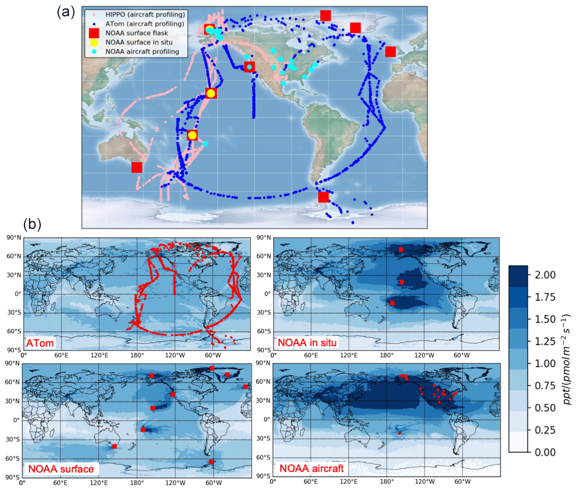
Figure 1Global atmospheric CFC-11 observations considered in this study (a), including selected flask measurements from the NASA HIPPO and ATom campaigns and observations from the NOAA global weekly surface flask sampling network, NOAA global in situ surface sampling network, and NOAA aircraft profiling sites. Panel (b) indicates the summed footprints between August 2016 and May 2018 from ATom (number of observations: 1003), NOAA weekly surface flask network (number of observations: 781), NOAA in situ network (only selected 1–2 samples d−1; number of observations: 2559), and NOAA biweekly–monthly aircraft profiling sites (only data above 1 km above ground were selected at North American sites; number of observations: 4824).
For measurements made during the HIPPO and ATom campaigns, we only include measurements below 8 km in the global inversions to minimize the influence of stratospheric loss on measured mole fractions and because high altitude samples typically have less emission information. Some samples obtained below 8 km still retained a notable stratospheric loss signal, and these data were also removed from further considerations on the basis of reduced mole fractions observed for N2O, which is useful for tracing stratospheric influence in an air parcel owing to its small atmospheric variability and high-precision measurements.
For data obtained in NOAA's regular flask-air sampling programs, the inversions included results from sites that are relatively far from recent anthropogenic emissions (i.e., sites many miles away from populated areas or that are not situated in the boundary layer) in order to capture emissions from broad regions. These observations include the weekly surface flask sampling at remote, globally distributed locations (Fig. 1) and aircraft profiling in Cook Islands and Alaska, USA, and above 1 km (above ground) over the contiguous USA (Fig. 1). Most of our aircraft profiling sampling was below 8 km above sea level.
To reduce the extremely large computing cost of footprint calculations for surface in situ sampling, we chose a subset of in situ samples for inversion analyses. We randomly selected one sample per day from sites such as Barrow, Alaska, USA (BRW), and Tutuila, American Samoa (SMO), and one daytime sample and one nighttime sample each day at Mauna Loa Observatory, Hawaii, USA (MLO). In situ measurements made at Summit, Greenland (SUM), were excluded due to poorer precision of CFC-11 measurements made at this station.
Although many of the observations we used were from remote Pacific and Atlantic ocean locations or from the free troposphere over North America, they did contain above-zero sensitivity to emissive signals transported from all the continents, as shown in their footprints (Fig. 1); but the overall sensitivity to emissions from South America, southern Africa, and Australia is low relative to North America, Europe, and Asia (Fig. 1). Thus, observational constraints on emissions from North America, Europe, and Asia are stronger and are less dependent on prior assumptions compared to those from South America, Africa, and Australia.
2.2.2 Footprint simulations
We used the HYSPLIT model driven by the global data assimilation system at a 0.5∘ resolution (HYSPLIT-GDAS0.5∘) to simulate footprints for our global inversion analyses. To determine an adequate number of particles needed for this global simulation, we tested running HYSPLIT backward for 45 d using 5000 and 10 000 particles for a subset of observations obtained from the second campaign during ATom (ATom-2). We compared the footprints from these two independent simulations, which are only different by < 0.05 % in the total summed sensitivities. Footprint distributions and magnitudes in individual time steps are also almost identical, suggesting that using 5000 particles was adequate for our global simulation.
To determine an adequate time duration for each HYSPLIT simulation, we compared footprints for observations with enhanced CFC-11 mole fractions versus those with relatively low mole fractions for observations made at different altitudes and latitudes from ATom-2. Our results show that, for observations in all altitude and latitude bins, those with enhanced CFC-11 mole fractions always had higher sensitivity to upwind populated regions in the first 20 d (Fig. S2); after that, the overall sensitivity was relatively small and constant likely due to evenly distributed particles throughout the troposphere beyond 20 d. This result suggests running HYSPLIT for more than 20 d was likely sufficient for capturing the major emission influence on atmospheric CFC-11 mole fraction observations made over the remote atmosphere. In the analysis presented here, sensitivities were derived with HYSPLIT-GDAS0.5∘ by tracking 5000 particles back in time for 30 d.
2.2.3 Estimation of background mole fractions
As described above, emissions were derived from measured mole fraction enhancements above background values. For each observation, the background mole fraction was estimated based on the 5000 HYSPLIT-GDAS0.5∘ back trajectories and a 4D background mole fraction field. We tested various approaches for constructing this 4D CFC-11 mole fraction field (see Supplement; Figs. S3 and S4). Here, we only describe the final choice selected for the inversion analysis. The final empirical 4D CFC-11 mole fraction field was constructed based on NOAA observations by propagating a subset of measured mole fractions of CFC-11 from the NOAA's global surface and ongoing airborne flask-air sampling programs back in time along the 5000 back trajectories for 10 d. Observations were included in the background estimate if the associated mole fraction was lower than the 70–80th percentile of all results in each 30∘ latitude × 3 km altitude box during the HIPPO period and the 40–50th percentile of all results in each box during the ATom period. These thresholds were chosen to ensure that the inversely derived global emissions in both periods were consistent with those derived from a global three-box model and a best estimate of the atmospheric CFC-11's lifetime (Montzka et al., 2021). Although the inversely derived global emission total was sensitive to the choice of the background threshold, the relative regional emission distribution or the fraction of regional emissions to the global emissions was not. By propagating this subset of observations back in time, it provided a 4D field of CFC-11 background mole fractions that we then averaged every 5∘ latitude × 20∘ longitude × 2 km altitude every month. This 4D empirical background did not account for the strong stratospheric influence on CFC-11 mole fractions at high altitudes (8–10 km) in the polar regions (> 60∘ N or > 60∘ S). Thus, we further scaled the CFC-11 mole fractions in these areas using the vertical gradients simulated by the Whole Atmosphere Community Climate Model (WACCM) (Davis et al., 2020; Marsh et al., 2013; Montzka et al., 2021; Ray et al., 2020).
From this 4D background mole fraction field, we sampled 5000 mole fraction estimates at the locations of the 5000 back trajectories at the end of the 30 d and then averaged these 5000 mole fraction estimates to obtain one background mole fraction for each observation. We examined the particle locations at the end of the 30 d using observations collected at 0–8 km from ATom-2. For the majority of these observations, 80 %–100 % of particles were located between 0 and 10 km at the end of the 30 d in the HYSPLIT back-trajectory runs. For particles that exited from the top at 10 km before 30 d, we sampled the mole fractions at 10 km when they exited the background mole fraction field.
2.2.4 Prior emissions
We constructed 11 different prior emission fields for inversion analyses in both the HIPPO and ATom periods (Fig. 2). The first prior emission field or “a priori” was constructed with assumed global CFC-11 emissions of 67 Gg yr−1. This global total was distributed around the globe in a 1∘ × 1∘ resolution based on a 1∘ × 1∘ gridded population density product from the Gridded Population of the World (GPW) v4 dataset (https://sedac.ciesin.columbia.edu/data/collection/gpw-v4, last access: 15 March 2019). The only exception is over the USA, where we used the 1∘ × 1∘ gridded annual emissions derived from Hu et al. (2017) for 2014. The second a priori emission has the same distribution as the first a priori emission, except the total emission magnitude was reduced by 40 % across the globe such that the global CFC-11 emissions in this scenario are 40 Gg yr−1. The other nine prior emission fields were constructed like the first a priori field but with an additional 20 Gg yr−1 of emissions imposed over North America, South America, Africa, Europe, Australia, boreal Asia, temperate eastern Asia, temperate western Asia, and tropical Asia. The 20 Gg yr−1 of emissions was added to those regions by a constant emission rate in picomoles per square meter per second (pmol m−2 s−1) across the grid cells having non-zero emissions in the first prior emissions. The regions specified as North America (NA), South America (SA), Africa (Af), Europe (Eu), Australia (Au), boreal Asia (BA), temperate eastern Asia (TEA), temperate western Asia (TWA), and tropical Asia (TA) are shown in Fig. 3. We named the 11 different prior emission fields as “population_GlobalEmission” or “population_GlobalEmission_ region” (Fig. 2), in which “population” represents their distribution; “GlobalEmission” represents the global emissions in gigagrams per year (Gg yr−1) in each prior; and “region” represents the location where the additional 20 Gg yr−1 of emissions was added. For example, “population_87_TEA” indicates a priori with global CFC-11 emissions of 87 Gg yr−1 and a distribution similar to population density; compared to the first a priori, this a priori had additional 20 Gg yr−1 emissions imposed over TEA.
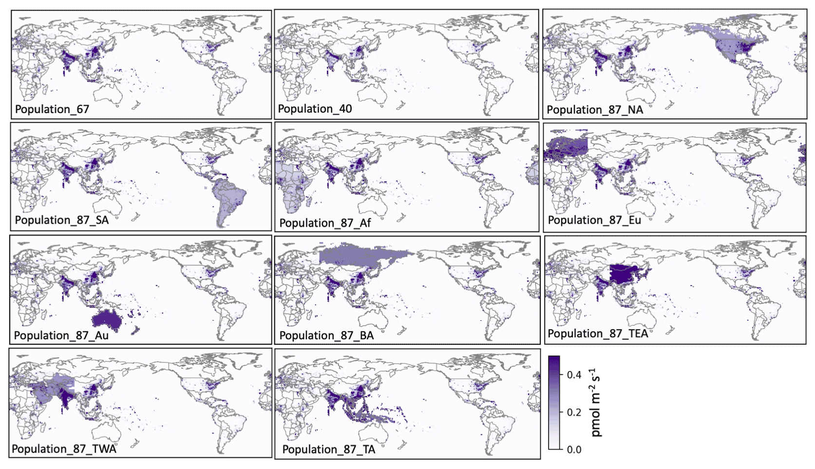
Figure 2Prior CFC-11 emissions used in this study. Priors of “population_67” and “population_40” have global CFC-11 emissions of 67 and 40 Gg yr−1. Compared to the prior “population_67”, priors of “population_87_NA”, “population_87_SA”, “population_87_Af”, “population_87_Eu”, “population_87_Au”, “population_87_BA”, “population_87_TEA”, “population_87_TWA”, and “population_87_TA” have a global emission total of 87 Gg yr−1 with an additional 20 Gg yr−1 of emissions imposed over North America, South America, Africa, Europe, Australia, boreal Asia, temperate eastern Asia, temperate western Asia, and tropical Asia, respectively.
We assume an exponential decaying covariance function in the errors of prior emissions (Hu et al., 2017).
where σq represents the 1σ error on a relative scale in the prior emissions; τl and τt denote the spatial and temporal correlation lengths of prior emission error (the 95 % correlation scales are approximately 3 τl and 3 τt); ht and hs are temporal intervals and spatial distance between state vectors; ht and hs can be calculated based on air sampling times and locations; σq, τl, and τt are dependent on prior emissions and were estimated by the maximum likelihood estimation; and σq was estimated in a range of 200 %–340 % given the nine different prior emission fields. The spatial and temporal correlation lengths were estimated as 2.5 km and 58 d. Prior uncertainty in regional emissions were then calculated by considering spatial and temporal correlations in space and time. The calculated 1σ uncertainty for the nine different priors is 20 %–60 % on a global scale and 20 %–120 % on a regional scale.
2.2.5 Inversion ensembles
We constructed 23 inversion ensembles for deriving global and regional emissions in the HIPPO and ATom periods. These 23 inversion ensembles included 20 different prior emission change scenarios between the HIPPO and ATom periods, two background CFC-11 mole fraction fields, and two sets of observations (“flask only” and “flask + in situ”) (Table S1). The 20 prior emission change scenarios assumed the following: (scenario 1) no increase in global CFC-11 emissions between the HIPPO and ATom periods (inversion ensemble IDs #1–#5 in Table S1); (scenario 2) a 20 Gg yr−1 increase in CFC-11 emissions between the HIPPO and ATom periods, with the increase being restricted to one of the following regions: North America, South America, Africa, Europe, Australia, boreal Asia, temperate eastern Asia, temperate western Asia, and tropical Asia (inversion ensemble IDs #6–#14, respectively, in Table S1); and (scenario 3) a 20 Gg yr−1 decrease in CFC-11 emissions between the HIPPO and ATom periods, with the decrease being restricted to one of the following regions: North America, South America, Africa, Europe, Australia, boreal Asia, temperate eastern Asia, temperate western Asia, and tropical Asia (inversion ensemble IDs #15–#23, respectively, in Table S1).
In our global inversions, we solved for monthly 1∘ × 1∘ emissions and their posterior covariances at 1∘ × 1∘ resolution. Because the uncertainty associated with the 1∘ × 1∘ emissions is large, we aggregated emissions and their posterior covariances into regional, continental, and global scales for the HIPPO and ATom periods, considering the cross correlation in errors among grid cells and across times for each inversion (Hu et al., 2017). In this study, we report the mean (μi) and 2 standard deviations (2σi) of posterior estimates for each inversion scenario, in which i denotes the inversion ID in Table S1. In the final results summarized in Table 1, we report two types of uncertainties. The first uncertainty is calculated as the percentile range 2.5–97.5 of the mean emissions (μi) derived from the 23 inversions, which are considered our “best estimates” of emissions. Uncertainties were also calculated considering the uncertainty (2σi) associated with each inversion. The lower bound of this second uncertainty was calculated as percentile 2.5 of , and the upper bound was calculated as percentile 97.5 of .
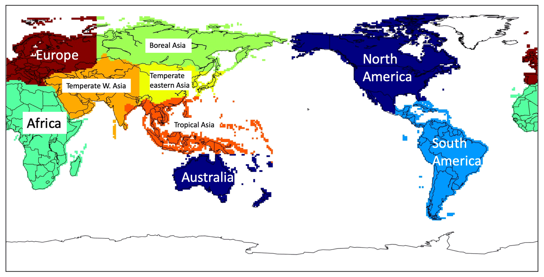
Figure 3Emissive regions defined for this analysis: North America, South America, Europe, Africa, Australia, and Asia; Asia was further divided into Boreal Asia, temperate eastern Asia, temperate western Asia, and Tropical Asia.
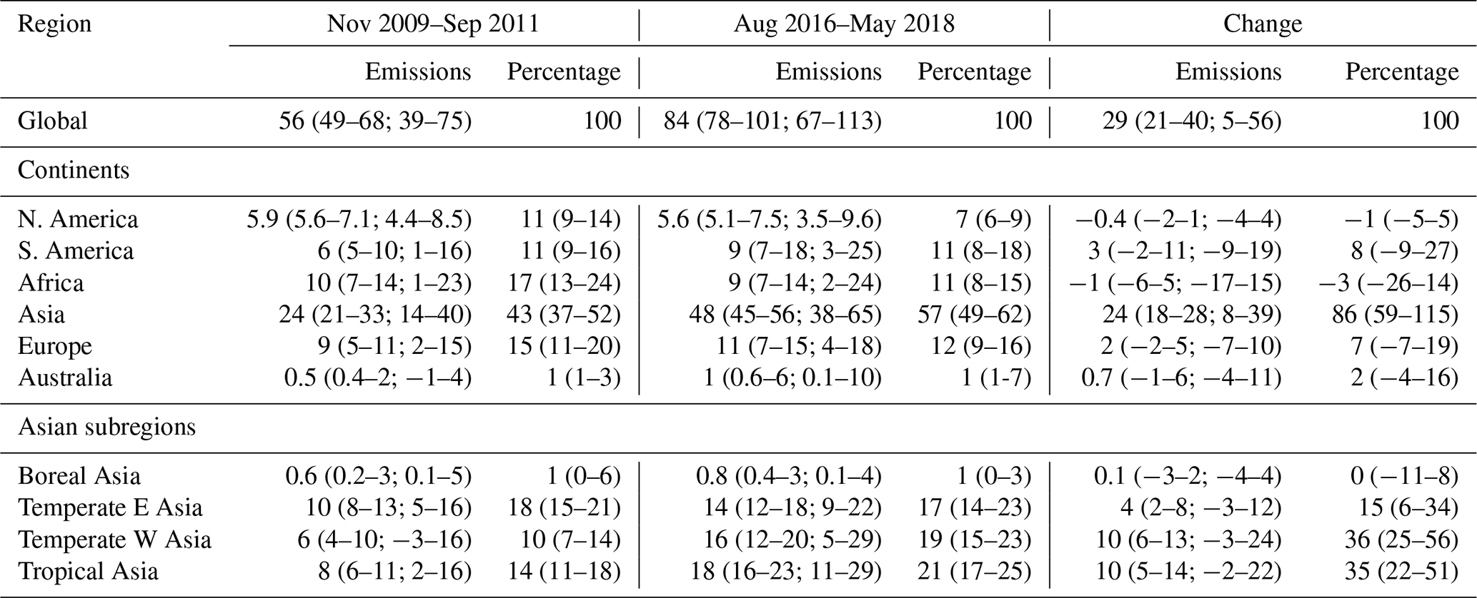
Table 1Global and regional emissions (Gg yr−1) derived from this analysis for November 2009–September 2011 and August 2016–May 2018 and the derived emission increases between the two periods (left columns). Two types of uncertainties are given in the parentheses. The first range indicates the percentile range 2.5–97.5 of the mean estimates derived from the 23 inversion ensembles. The second range indicates the percentile range 2.5–97.5 of the 23 inversions, considering the mean and 2σ errors from each inversion. The right columns indicate the percentage contributions of regional emissions to the global CFC-11 emissions and emission changes; values in the parentheses indicate the percentile range 2.5–97.5 of the mean regional emissions relative to the mean global emissions among the 23 inversion ensembles.
3.1 Increase in CFC-11 emissions between the HIPPO and ATom periods observed in remote atmospheric observations
The global increase in CFC-11 emissions between 2012 and 2017 was previously derived from the slowdown in the decline of atmospheric CFC-11 mole fractions observed at the Earth's surface (Montzka et al., 2018, 2021) and is also shown in Fig. 4 here. Besides at the Earth's surface, a similar magnitude of this slowdown in atmospheric CFC-11 mole fraction decline is also apparent throughout the free troposphere in the aircraft profiles obtained during the HIPPO and ATom campaigns, each of which involved sampling deployments spread over approximately 2 years (Fig. 4). Here, we calculated the CFC-11 growth rates averaged in each 30∘ latitude × 2 km altitude box during HIPPO campaigns and during ATom campaigns separately for samples collected above the Pacific Ocean basin. During HIPPO, we calculated the average mole fraction differences in each 30∘ latitude × 2 km altitude box between HIPPO-3 (March 2010–April 2010) and HIPPO-4 (June 2011–July 2011) and normalized their time interval to obtain annual growth rates, whereas we calculated annual growth rates during ATom using the ATom-1 (July 2016–August 2016) and ATom-4 (April 2018–May 2018) data. The reason to choose HIPPO-3, HIPPO-4, ATom-1, and ATom-4 for this calculation is to ensure annual growth rates were calculated from data collected in similar seasons so that the impact of seasonal variations in atmospheric CFC-11 mole fractions on the calculated annual growth rates was minimized (Fig. S5). Results suggest a median growth rate of −2.5 ppt yr−1 (parts per trillion per year) between 60∘ S and 90∘ N in the troposphere during the HIPPO period and a median growth rate of −0.7 ppt yr−1 during the ATom period (Fig. 4), indicating a significant increase in CFC-11 growth rates in the troposphere between the HIPPO and ATom periods. The impact of the atmospheric CFC-11 seasonal cycle measured at the surface on the calculated changes in annual growth rates between both periods is about ± 0.1 ppt. Besides the seasonal cycle of atmospheric CFC-11 mole fractions, the quasi-biennial oscillation (QBO) can also influence atmospheric trace gas mole fractions in the troposphere (Ray et al., 2020) and thus their growth rates. However, this influence was smaller than the increase in the annual growth rates between the HIPPO and ATom periods, as quantified in Montzka et al. (2021).
After subtracting background CFC-11 mole fractions from the selected global CFC-11 observations, enhancements approaching 3 ppt were found in air above the Pacific Ocean basin during both sampling periods by all measurement methods (on board the HIPPO and ATom aircraft surveys, from the global weekly flask sampling, and from the selected daily to “every other day” in situ sampling) (Fig. 5). Relatively larger enhancements were more frequently measured during the ATom period than during the HIPPO period (Fig. 5). However, the average increase in enhancements of the atmospheric CFC-11 mole fractions measured during ATom were 0.2–0.3 ppt higher than those observed during the HIPPO campaign (Fig. 5). The 0.2–0.3 ppt increase in the atmospheric CFC-11 enhancements was also independently measured by the global weekly flask sampling and in situ sampling networks over the Pacific Ocean basin (Fig. 5). Results from HIPPO and ATom suggest that increased mole fraction enhancements over the Pacific Ocean basin existed primarily between 0 and 60∘ N (Fig. 5), where the lower and middle tropospheric air mainly contains emissive signals from Eurasia, western North America, and tropical America (Fig. S6). Furthermore, during ATom, CFC-11 enhancements measured in the Pacific Ocean basin were larger than those measured in the Atlantic Ocean basin (Fig. 5), suggesting regions immediately upwind of the Pacific Ocean were emitting more CFC-11 than regions upwind of the Atlantic Ocean (Fig. 1b) during the ATom period.
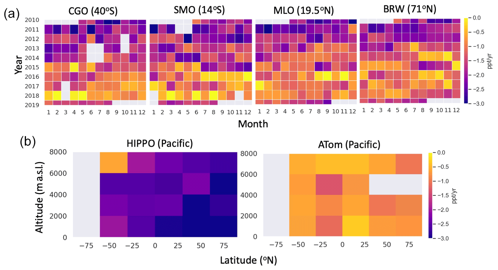
Figure 4Annual growth rates of atmospheric CFC-11 measured at four surface flask sampling sites over the Pacific Ocean basin from 2010–2019 (a) and CFC-11 growth rates measured during the selected HIPPO and ATom aircraft profiling surveys that took place during November 2009–September 2011 and August 2016–May 2018, respectively (b). Each grid cell indicates an annual difference relative to the prior year for that given month (a) or location (b). Gray cells indicate periods or locations with no data. The four surface sites plotted in panel (a) are Cape Grim, Tasmania, Australia (CGO), Tutuila, American Samoa (SMO), Mauna Loa, Hawaii, United States (MLO), and Point Barrow, Alaska, United States (BRW).
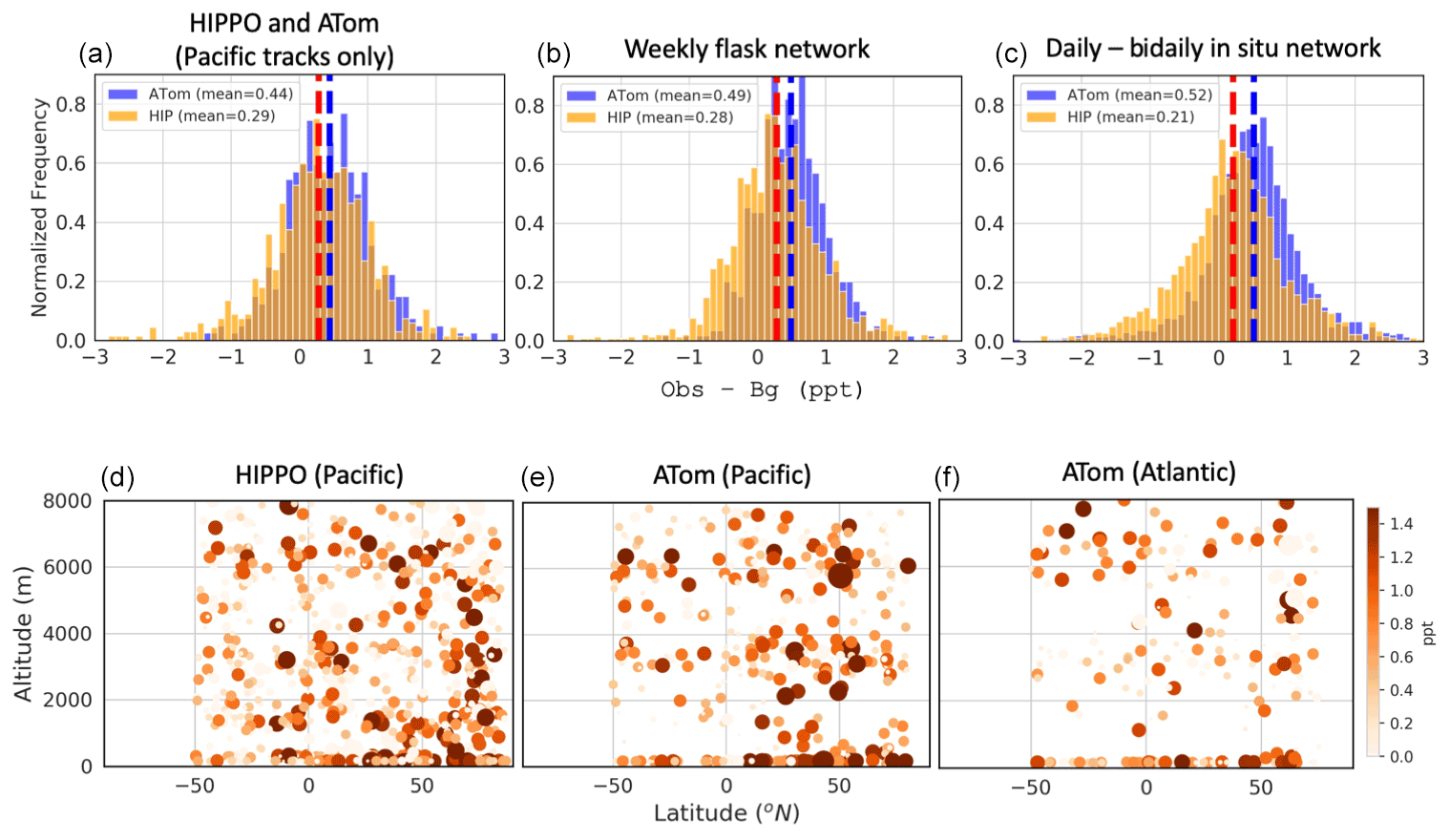
Figure 5Enhancements of CFC-11 mole fractions relative to background air mole fractions, measured by three independent networks during November 2009–September 2011 (HIPPO period) and August 2016–May 2018 (ATom period). (a) Histograms of enhancements of CFC-11 mole fractions measured from flasks collected over the Pacific Ocean basin during the HIPPO and ATom campaigns (a, d), in flasks collected in the NOAA weekly surface sampling network during those periods (b, e), and measured from the NOAA in situ sampling network in both periods (c, f). Orange bars indicate normalized frequencies of enhancements observed in the HIPPO period, whereas blue bars indicate normalized frequencies of enhancements observed in the ATom period. Dashed red and blue lines denote the mean mole fractions observed during HIPPO and ATom periods. (b) Atmospheric CFC-11 mole fraction enhancements measured from flasks above the Pacific Ocean basin during HIPPO (a, d) and ATom (b, e), as well as above the Atlantic Ocean basin during ATom (c, f). Both color shading and size of the symbols are proportional to the magnitude of mole fraction enhancements.
3.2 Regional emissions derived from HIPPO and ATom global inversions
3.2.1 The base scenarios with only flask-air measurements
To quantitatively understand what measured atmospheric CFC-11 variability implies for global and regional CFC-11 emissions, we conducted Bayesian inversions as described in Sect. 2. We first only used the flask-air measurements made by the two GCMS instruments. These measurements include samples collected during HIPPO and ATom, the global weekly flask-air sampling program, and the regular aircraft flask-air sampling program located primarily over North America. The inversions derived from these flask-air measurements are referred to here as “flask-only inversions”. In this first base scenario, we used the same prior emissions with global CFC-11 emissions of 67 Gg yr−1 (“population_67” shown in Fig. 2) for both HIPPO and ATom periods (Table S1). The global emissions derived from this scenario (67 ± 7 and 87 ± 9 Gg yr−1 for the HIPPO and ATom periods) were based on background estimates that were calibrated against the global three-box model results such that the global CFC-11 emissions derived from the grid-scale inversions were consistent with those from the global three-box model with an atmospheric lifetime of 52 years reported by Montzka et al. (2021).
An inverse analysis of the flask data obtained during the HIPPO and ATom periods suggest changes in the total magnitude and distribution of CFC-11 emissions from 2010–2018. Significant emission increases were derived for Asia by an amount that suggests it was primarily responsible for the global CFC-11 emission increase from 2010–2018. During the HIPPO period (November 2009–September 2011), Asia emitted 35 (±5) Gg yr−1 of CFC-11, accounting for 50 % of global CFC-11 emissions, whereas Asian annual CFC-11 emissions increased to 51 (±8) Gg yr−1 during the ATom period in August 2016–May 2018, equal to 60 % of the global CFC-11 emissions at that time. Results from this scenario yield an increase in CFC-11 emissions from Asia during these two periods of 16 (±10) Gg yr−1, which accounted for 80 %–90 % of global CFC-11 emission increases during these specific years (19±12 Gg yr−1) (Fig. 6), as derived from this scenario.
Our inversion results also suggest that the Asian CFC-11 emissions and emission increases were primarily contributed by temperate eastern Asia, temperate western Asia, and tropical Asia in approximately equal amounts (Fig. 6). Correlations (as r2) or covariations in the posterior emissions among these three Asian subregions were less than 0.1, suggesting the inversion was able to separate regional total emissions from these three subregions, although the derived analytical uncertainties associated with emissions at the subregional level are overlapping (Fig. 6).
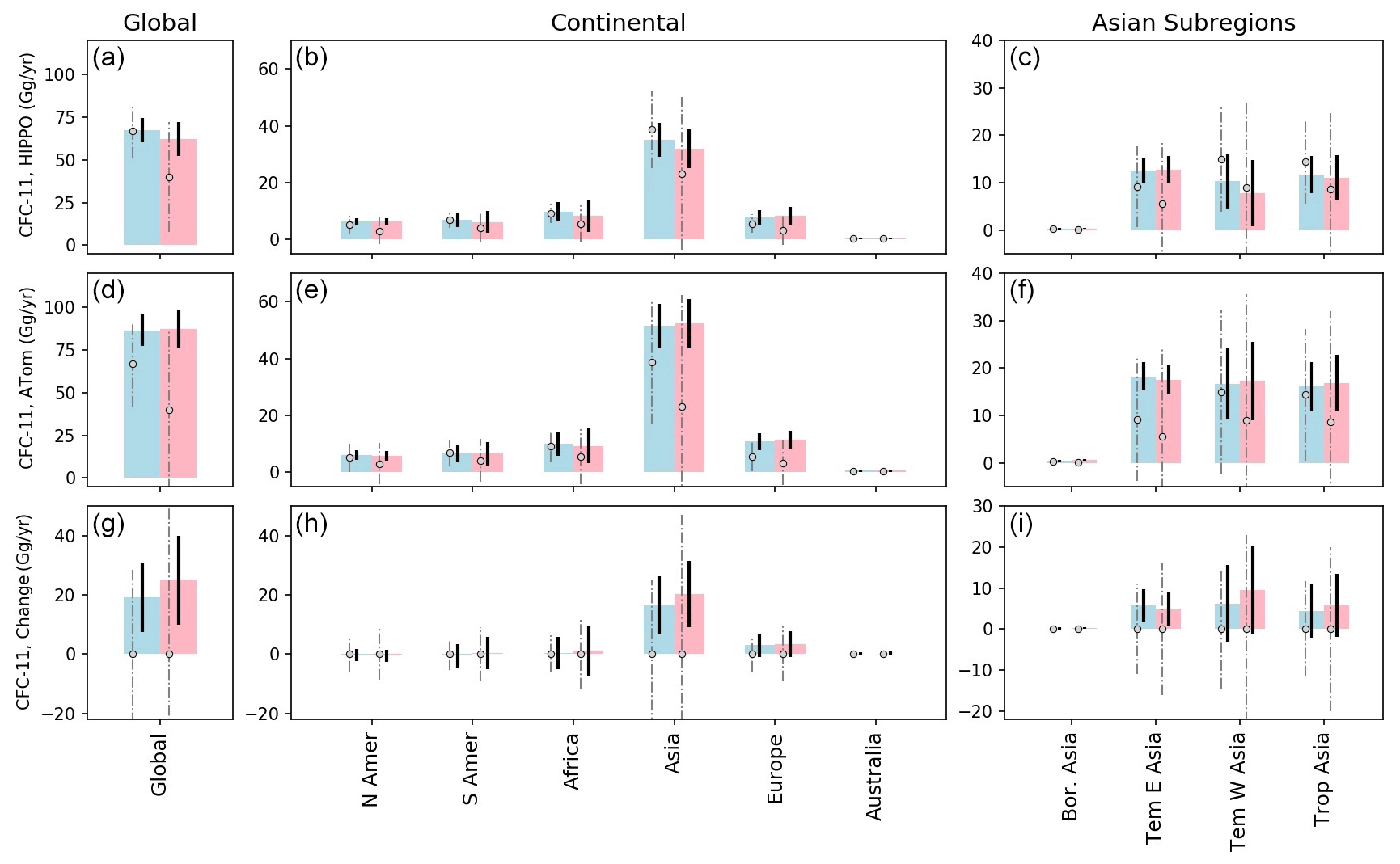
Figure 6Prior (circles) and posterior (bars) CFC-11 emissions derived for the globe, continents, and Asian subregions from the “flask-only” inversions for the HIPPO period (a–c) and the ATom period (d–f), as well as emission differences between the two periods (g–i). In each region and from the left to right, open circles denote the two assumed prior emissions (“population_67” and “population 40”) with zero changes between the HIPPO and ATom periods. Dashed gray lines indicate 2σ prior uncertainties. Light blue and pink bars correspond to posterior emissions derived from the two different priors. Black error bars of CFC-11 emissions derived for the HIPPO and ATom periods (a–f) indicate 2σ posterior uncertainties derived from individual inversions. Error bars for the derived CFC-11 emission changes (g–i) between the HIPPO and ATom periods were calculated from the square root of the sum squared errors shown in (a)–(c) and (d)–(f).
Emissions derived for North America, South America, Africa, and Europe were 5–15 Gg yr−1 for each region in both the HIPPO and ATom periods. Emissions derived for Australia were less than 1 Gg yr−1. Changes in CFC-11 emissions between both periods derived for all seven of these continents were smaller than their associated uncertainties in this scenario.
With “flask-only” observations, we also tested the sensitivity of posterior regional emissions to the prior emission magnitude. Here, we considered the second “population-density” prior with substantially lower global total CFC-11 emissions of 40 Gg yr−1 for both periods (“population_40”) (Table S1). Derived regional emissions from this second scenario were consistent with results discussed in the first scenario in both the distribution and total magnitude of posterior emissions.
To assess how much constraint the selected atmospheric observations added to regional emission estimates, we calculated the uncertainty reduction between the prior and posterior emission uncertainties. Note that the uncertainty reduction is generally correlated with the sensitivity of atmospheric observations to surface emissions (or footprint) and is dependent on how good the prior emissions are. As expected, the uncertainty reduction is indeed the largest (50 %–80 %) over North America and Asia (Table S2; Fig. 6), where our observations have the strongest sensitivity, and the smallest over South America, Africa, and Australia (3 %–50 %) (Fig. 6; Table S2), where our observations have the lowest sensitivity (Fig. 1).
3.2.2 Inversions using more observations, different prior assumptions, and an alternative background mole fraction field
To increase the observational constraints in the global CFC-11 inversion, we then included additional observations from the in situ CFC-11 measurements (Fig. 1; inversion ID = 3–4 in Table S1). The derived posterior emissions with this expanded observational dataset (and with the same population-based priors and background estimates) show slightly higher global emissions, especially from tropical Asia, during the ATom period (Fig. 7). Besides the inclusion of additional observations, we also considered an alternative background estimate (background 2) that was calibrated to the global CFC-11 emission estimates with alternative atmospheric lifetimes (54 and 56 years) (Montzka et al., 2021) (inversion ID = 5 in Table S1). As expected, the derived global and regional emissions were lower with a background calibrated to a longer atmospheric lifetime. However, the derived regional contributions to the global CFC-11 emissions and emission changes between the HIPPO and ATom periods were consistent with results considering a shorter lifetime (Fig. 7).
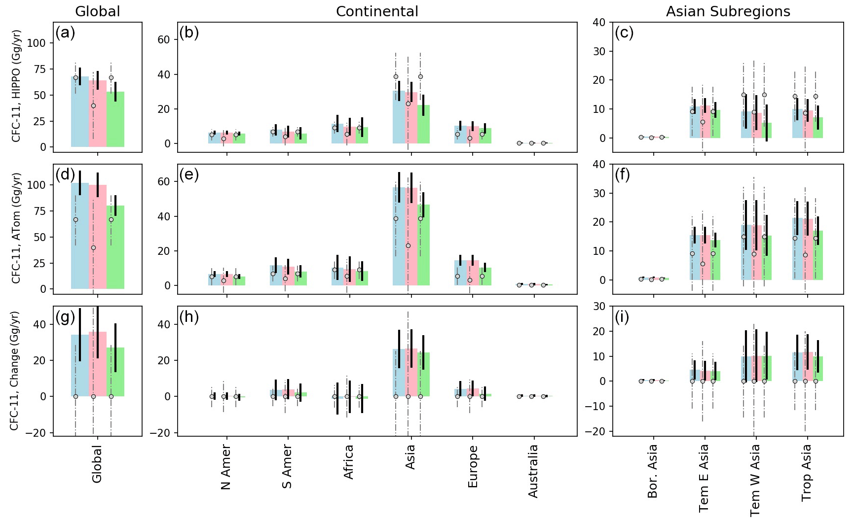
Figure 7Prior (circles) and posterior (bars) CFC-11 emissions derived for the globe, continents, and Asian subregions from the “flask + in situ” inversions for the HIPPO period (a–c) and the ATom period (d–f), as well as emission differences between the two periods (g–i). In each region and from the left to right, open circles denote the three assumed prior emissions (“population_67”, “population 40”, and “population_67”) with zero changes between the HIPPO and ATom periods. Light blue, pink, and green bars indicate posterior emissions derived from the three priors and two different backgrounds, as described in inversion ID = 3–5 in Table S1.
Results discussed so far are based on prior emissions that do not change between the HIPPO and ATom periods for all regions considered. The remaining questions are as follows. (1) Are the resulting near-zero emission changes over North America, South America, Africa, Europe, and Australia due to the influence from prior assumption (zero emission changes in the prior) or are they the result of observational constraints? (2) To what degree are derived Asian emissions and emission changes dependent on assumptions of prior emission changes? To address these questions, we constructed 18 additional scenarios (as part of the 23 scenarios described in Sect. 2.2.5) that assumed 20 Gg yr−1 CFC-11 emission increases in the prior emissions between the HIPPO and ATom periods (inversion ID = 6–14 in Table S1) or 20 Gg yr−1 CFC-11 emission decreases between the HIPPO and ATom periods (inversion ID = 15–23 in Table S1). In the first nine cases, we considered the same population-based prior with global CFC-11 emissions of 67 Gg yr−1 during the HIPPO period (prior = “population_67”), whereas during the ATom period, we assumed there was an increase of 20 Gg yr−1 of CFC-11 emissions over individual continents (North America, South America, Africa, Europe, and Australia) or individual Asian subregions (boreal Asia, temperate eastern Asia, temperate western Asia, and tropical Asia) (prior = “population_87_region”). In the latter nine cases, we considered opposite scenarios, in which we assumed 67 Gg yr−1 of emissions during the ATom period (prior = “population_67”) and 87 Gg yr−1 of emissions during the HIPPO period (prior = “population_87_region”) so that emissions over individual continents or individual Asian subregions had a 20 Gg yr−1 decrease between both periods (Fig. 8). Note that, given it is known there was a global increase in CFC-11 emissions from 2010–2018 (Montzka et al., 2018, 2021) and 60 ± 40 % of this global increase was from eastern mainland China (Park et al., 2021; Rigby et al., 2019), many of the assumed 18 prior emission change cases were quite unrealistic. However, such extreme cases helped for estimating uncertainties that truly reflect the capability of the selected atmospheric measurements for constraining continental and regional emissions and their change through time. In all of the 18 extreme cases, regional emissions and emission changes derived for the northern hemispheric lands, i.e., Asia, North America, and Europe, were consistent (Fig. 8). Derived regional emissions and emission changes for the southern hemispheric lands, such as South America, Africa, Australia, however, show a strong dependence on prior assumptions, especially during the ATom period (Fig. 8). The strong dependence of inversion-derived emissions over the southern hemispheric lands were due to large sampling gaps and small sensitivity to emissions from these regions (Fig. 1).
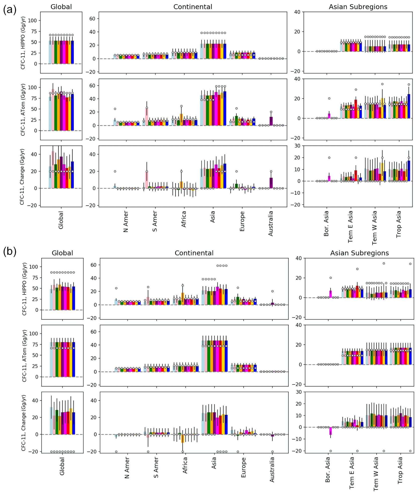
Figure 8Testing the sensitivity of assumed prior emission changes on the inversion-derived emission changes. (a) Assume a 20 Gg yr−1 emission increase between the HIPPO and ATom periods in individual continents and Asian subregions. (b) Assume a 20 Gg yr−1 emission decrease between the HIPPO and ATom periods in individual continents and Asian subregions. Similar to Fig. 7, posterior CFC-11 emissions were derived from the “flask + in situ” inversions for the HIPPO and the ATom periods. In each region and from the left to right, open circles denote the prior emissions as described for inversion ID = 6–14 in Table S1 for panel (a) and for inversion ID = 15–23 in Table S1 for panel (b); different colored bars indicate the corresponding posterior emissions derived from inversion ID = 6–14 (a) and ID = 15–23 (b) as described in Table S1.
Summarizing emissions derived from all 23 inversion ensembles (Table 1; Figs. 6–8), our results suggest the relatively remote observations provide important constraints on regional emissions from North America, Asia, and Europe as the derived ranges of posterior emissions were smaller than the ranges of prior emissions considered for these regions (Figs. 6–8). The only continent that shows a statistically significant increase in CFC-11 emissions is Asia, where the best estimate of these 23 cases suggests an increase of 24 (18–28) Gg yr−1 of CFC-11 emissions (the percentile range 2.5–97.5) (Table 1), accounting for 86 (59–115) % of the global CFC-11 emission increases between the HIPPO and ATom periods. All the best estimates from the 23 inversion ensembles suggest CFC-11 emission increases not only from temperate eastern Asia but also from temperate western Asia and tropical Asia. However, if we consider the entire range of uncertainties (the range of best estimates and 2σi errors from each inversion; Table 1), the derived emission increases were statistically insignificant at the subregion level (i.e., temperate eastern Asia, temperate western Asia, and tropical Asia).
Our results also suggest inverse modeling of the relatively remote observations we considered here provided only weak constraints on emissions from the southern hemispheric continents, i.e., South America, Africa, and Australia. Although we cannot eliminate the possibility of some increase in CFC-11 emissions from these southern hemispheric regions based on atmospheric inversion analyses alone, they did not account for the majority of the emission increase. This is because during 2010–2018, when the global CFC-11 emissions increased, so did the north-to-south mole fraction difference between the hemispheres (Montzka et al., 2021), which indicates the emission increase occurred predominantly in the northern hemisphere.
3.2.3 Comparison of regional emission estimates from other top-down analyses
Our regional emission estimates of CFC-11 from the global atmospheric CFC-11 measurements made far away from the emissive regions are in a broad agreement with those estimated from atmospheric observations made closely downwind of the emissive regions (Table 2), which included the analyses of atmospheric CFC-11 enhancements observed closely downwind of emissive regions that were 1–2 orders of magnitude larger than those used in the present inversion analysis (Park et al., 2021; Rigby et al., 2019; Hu et al., 2017; Fraser et al., 2020). Emissions estimated for eastern mainland China using measurements made in South Korea were 5–13 Gg yr−1 during 2010–2011 and 12–20 Gg yr−1 during 2016–2017, considering the full range of estimates from multiple inversion systems with different transport simulations (Park et al., 2021). CFC-11 emission estimates for eastern China based on measurements made in Taiwan were 14–23 Gg yr−1 during 2014–2018 (Adcock et al., 2020). In the current analysis, we estimated that CFC-11 emissions from temperate eastern Asia were 5–16 Gg yr−1 during November 2009–September 2011 and 9–22 Gg yr−1 during August 2016–May 2018, which agree well with the published analyses over eastern China, although our definition of temperate eastern Asia is slightly different from the regions defined in Rigby et al. (2019), Adcock et al. (2020), and Park et al. (2021).
Table 2Comparison of regional emissions derived from this study and reported by previous top-down analyses.
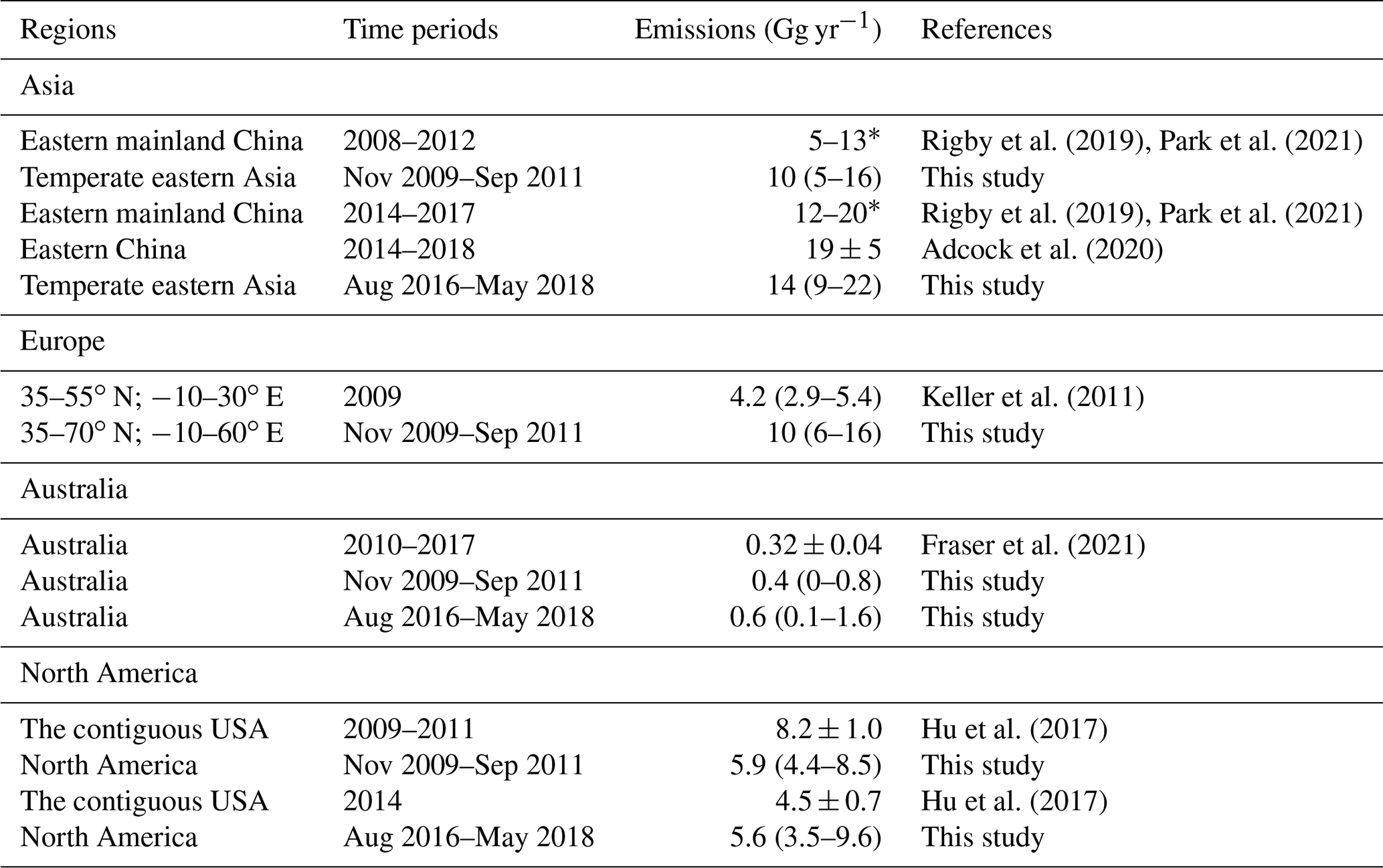
* Values were taken from the reported inversion ensemble spread.
Previously, we estimated the US emissions of CFC-11 between 2008 and 2014 with more extensive atmospheric measurements made from towers and aircraft sites from all vertical levels over North America (Hu et al., 2017). In this analysis, we only used a subset of observations (only aircraft observations above 1 km above ground) and a coarser resolution of transport models in the global inversion. While the North American CFC-11 emissions derived here are likely not as accurate, they did agree within uncertainties with our previous US estimates (Table 2).
Furthermore, CFC-11 emissions derived for Australia are also comparable with estimates reported by Fraser et al. (2020) using measurements made in Australia (Table 2). Both suggest CFC-11 emissions from Australia were less than 1 Gg yr−1 between 2009 and 2018, and contributions from Australia to global CFC-11 emissions and emission changes were very small.
Besides temperate eastern Asia, North America, and Australia, we also compared our derived European CFC-11 emissions for November 2009–September 2011 with the value reported by Keller et al. (2011) for western Europe in 2009. Our best estimate of 4.2 (2.9–5.4) Gg yr−1 for all of Europe was about twice as large as that reported by Keller et al. (2011) for western Europe, which only accounted for 40 % of the area we considered for all of Europe. If aggregating emissions from only grid cells considered in Keller et al. (2011), the aggregated total emissions would be similar to the value reported by Keller et al. (2011), although both studies focused on two different time periods (Table 2).
Other than the regions mentioned above, previous emission estimates for the rest of the world are quite limited. Only one study quantified CFC-11 emissions from the northern and central areas of India in June 2016, reporting emissions of ∼ 1–3 Gg yr−1 (Say et al., 2019). It is hard to make a fair comparison with our analysis, given its short analysis period and a much smaller area than our defined temperate western Asian region (Fig. 4). However, there is observational evidence indicating likely strong regional emissions and a regional emission increase over temperate western Asia between 2012 and 2017. This was shown as substantially enhanced CFC-11 mole fractions observed in temperate western Asia for flask measurements made during 2012–2018 (Simpson et al., 2019) and the slowdown of atmospheric CFC-11 decline retrieved from satellite remote sensing measurements (Chen et al, 2020). Furthermore, in situ measurements made in tropical Asia in 2017 (Lin et al., 2019) also indicate likely strong regional emissions of CFC-11 over this area.
We used global atmospheric CFC-11 measurements primarily made over the Pacific and Atlantic ocean basins and in the free troposphere over North America to quantify changes in continental-scale emissions between November 2009–September 2011 and August 2016–May 2018. These two periods covered the times when global CFC-11 emissions were at their minimum and maximum, respectively, in recent years, at least before the sharp decline noted after 2018 (Montzka et al., 2021). Atmospheric CFC-11 measurements made during both the HIPPO and ATom campaigns confirm that the slowdown of atmospheric CFC-11 mole fraction decline between 2009 and 2018 was present throughout the troposphere. The ATom campaign data further display larger atmospheric CFC-11 enhancements in flights, particularly over the Pacific Ocean basin as compared to the Atlantic Ocean basin, suggesting larger emissions in regions immediately upwind of the Pacific Ocean than the Atlantic Ocean during 2016–2018.
Inverse modeling of these global atmospheric CFC-11 measurements suggests three Asian regions were primarily responsible for the global CFC-11 emission changes from 2009–2011 to 2016–2018 in all of the 23 inversion ensembles, including various extreme initial assumptions of regional CFC-11 emission changes (±20 Gg yr−1) between both periods. Our results suggest that, during November 2009–September 2011, Asia emitted 24 (14–40) Gg yr−1 of CFC-11, accounting for 43 (37–52) % of the global emissions (Table 1), whereas the Asian CFC-11 emission increase to 48 (38–65) Gg yr−1 or 57 (49–62) % of the global emissions during August 2016–May 2018 (Table 1). In both periods, substantial CFC-11 emissions were derived for temperate eastern Asia, temperate western Asia, and tropical Asia. Besides eastern mainland China, our results suggest there could be increases in CFC-11 emissions from temperate western Asia and tropical Asia from 2010–2018, considering the range of best estimates from the 23 inversion ensembles. In contrast to Asia, other continents accounted for relatively smaller fractions of global CFC-11 emissions in both periods. For continents in the Southern Hemisphere, our inversion analyses only provide weak constraints on the CFC-11 emission changes between 2012 and 2018. However, significant increases in CFC-11 emissions from these regions are unlikely, provided the observed concurrent increase in the north-to-south difference in CFC-11 surface mole fractions.
NOAA atmospheric observations are available at the NOAA/GML website (https://gml.noaa.gov/hats/, NOAA GML, 2022). Data collected from ATom are available via https://espo.nasa.gov/atom/content/ATom and https://doi.org/10.3334/ORNLDAAC/1581 (Wofsy et al., 2018). Data collected from HIPPO are available via https://www.eol.ucar.edu/field_projects/hippo (NCAR/UCAR Earth Observing Laboratory, 2022). Inversion-derived continental fluxes were tabulated and described in this paper. All analysis tools and computing code used in this analysis will be available by contacting Lei Hu (lei.hu@noaa.gov).
The supplement related to this article is available online at: https://doi.org/10.5194/acp-22-2891-2022-supplement.
LH and SAM designed the analysis. LH conducted inversions and wrote the paper. SAM led the NOAA global flask measurements, as well as HIPPO and ATom GCMS measurements, and provided substantial input on the analyses and edits of this paper. FM and EH collected HIPPO and ATom flask-air samples. GD led the CATS measurements and prepared CATS data for this analysis. MCS made the NOAA flask measurements. LH and KT computed HYSPLIT footprints. RWP conducted the WACCM simulations and provided the model results. KM conducted NOAA aircraft data quality assurance and quality control (QA/QC). CS led the NOAA aircraft sampling network. IV led the Perseus GCMS flask measurements. DN helped with data QA/QC for CFC-11 flask measurements. BH led the calibration for NOAA measurements. SW led the HIPPO and ATom campaigns. All authors contributed to the editing of this paper.
The contact author has declared that neither they nor their co-authors have any competing interests.
Publisher’s note: Copernicus Publications remains neutral with regard to jurisdictional claims in published maps and institutional affiliations.
This work was funded by the NASA Earth Venture Atmospheric Tomography (ATom) mission (NNX16AL92A) and in part by the NOAA cooperative agreement with CIRES (NA17OAR4320101). We thank our retired colleagues Ben Miller for his development of the Perseus (PR1) GCMS instrument and James Elkins for his leadership and contribution to the HIPPO and ATom flask sampling and measurements. We also thank Arlyn Andrews, Ariel Stein, and Christopher Loughner for suggestions on HYSPLIT simulations.
This research has been supported by NASA Earth Venture Atmospheric Tomography (ATom) mission (grant no. NNX16AL92A).
This paper was edited by Jens-Uwe Grooß and reviewed by two anonymous referees.
Adcock, K. E., Ashfold, M. J., Chou, C. C. K., Gooch, L. J., Mohd Hanif, N., Laube, J. C., Oram, D. E., Ou-Yang, C.-F., Panagi, M., Sturges, W. T., and Reeves, C. E.: Investigation of East Asian Emissions of CFC-11 Using atmospheric observations in Taiwan, Environ. Sci. Technol., 54, 3814–3822, https://doi.org/10.1021/acs.est.9b06433, 2020.
Bourgeois, I., Peischl, J., Thompson, C. R., Aikin, K. C., Campos, T., Clark, H., Commane, R., Daube, B., Diskin, G. W., Elkins, J. W., Gao, R. S., Gaudel, A., Hintsa, E. J., Johnson, B. J., Kivi, R., McKain, K., Moore, F. L., Parrish, D. D., Querel, R., Ray, E., Sánchez, R., Sweeney, C., Tarasick, D. W., Thompson, A. M., Thouret, V., Witte, J. C., Wofsy, S. C., and Ryerson, T. B.: Global-scale distribution of ozone in the remote troposphere from the ATom and HIPPO airborne field missions, Atmos. Chem. Phys., 20, 10611–10635, https://doi.org/10.5194/acp-20-10611-2020, 2020.
Chen, X., Huang, X., and Strow, L. L.: Near-Global CFC-11 trends as observed by Atmospheric Infrared Sounder From 2003 to 2018, J. Geophys. Res.-Atmos., 125, e2020JD033051, https://doi.org/10.1029/2020JD033051, 2020.
Davis, N. A., Davis, S. M., Portmann, R. W., Ray, E., Rosenlof, K. H., and Yu, P.: A comprehensive assessment of tropical stratospheric upwelling in the specified dynamics Community Earth System Model 1.2.2 – Whole Atmosphere Community Climate Model (CESM (WACCM)), Geosci. Model Dev., 13, 717–734, https://doi.org/10.5194/gmd-13-717-2020, 2020.
Dhomse, S. S., Feng, W., Montzka, S. A., Hossaini, R., Keeble, J., Pyle, J. A., Daniel, J. S., and Chipperfield, M. P.: Delay in recovery of the Antarctic ozone hole from unexpected CFC-11 emissions, Nat. Commun., 10, 5781, https://doi.org/10.1038/s41467-019-13717-x, 2019.
Engel, A., Rigby, M., Burkholder, J. B., Fernandez, R. P., Froidevaux, L., Hall, B. D., Hossaini, R., Saito, T., Vollmer, M. K., and Yao, B.: Update on Ozone-Depleting Substances (ODSs) and Other Gases of Interest to the Montreal Protocol, chap. 1, in: Scientific Assessment of Ozone Depletion: 2018, Global Ozone Research and Monitoring Project — Report No. 58 World Meteorological Organization, Geneva, Switzerland, 2018.
Fraser, P. J., Dunse, B. L., Krummel, P. B., Steele, L. P., Derek, N., Mitrevski, B., Allison, C. E., Loh, Z., Manning, A. J., Redington, A., and Rigby, M.: Australian chlorofluorocarbon (CFC) emissions: 1960–2017, Environ. Chem., 17, 525–544, https://doi.org/10.1071/EN19322, 2020.
Hu, L., Montzka, S. A., Miller, J. B., Andrews, A. E., Lehman, S. J., Miller, B. R., Thoning, K., Sweeney, C., Chen, H., Godwin, D. S., Masarie, K., Bruhwiler, L., Fischer, M. L., Biraud, S. C., Torn, M. S., Mountain, M., Nehrkorn, T., Eluszkiewicz, J., Miller, S., Draxler, R. R., Stein, A. F., Hall, B. D., Elkins, J. W., and Tans, P. P.: U.S. emissions of HFC-134a derived for 2008–2012 from an extensive flask-air sampling network, J. Geophys. Res.-Atmos., 120, 801–825, 2014JD022617, https://doi.org/10.1002/2014JD022617, 2015.
Hu, L., Montzka, S. A., Miller, B. R., Andrews, A. E., Miller, J. B., Lehman, S. J., Sweeney, C., Miller, S. M., Thoning, K., Siso, C., Atlas, E. L., Blake, D. R., de Gouw, J., Gilman, J. B., Dutton, G., Elkins, J. W., Hall, B., Chen, H., Fischer, M. L., Mountain, M. E., Nehrkorn, T., Biraud, S. C., Moore, F. L., and Tans, P.: Continued emissions of carbon tetrachloride from the United States nearly two decades after its phaseout for dispersive uses, P. Natl. Acad. Sci. USA, 113, 2880–2885, https://doi.org/10.1073/pnas.1522284113, 2016.
Hu, L., Montzka, S. A., Lehman, S. J., Godwin, D. S., Miller, B. R., Andrews, A. E., Thoning, K., Miller, J. B., Sweeney, C., Siso, C., Elkins, J. W., Hall, B. D., Mondeel, D. J., Nance, D., Nehrkorn, T., Mountain, M., Fischer, M. L., Biraud, S. C., Chen, H., and Tans, P. P.: Considerable contribution of the Montreal Protocol to declining greenhouse gas emissions from the United States, Geophys. Res. Lett., 44, 2017GL074388, https://doi.org/10.1002/2017GL074388, 2017.
Keeble, J., Abraham, N. L., Archibald, A. T., Chipperfield, M. P., Dhomse, S., Griffiths, P. T., and Pyle, J. A.: Modelling the potential impacts of the recent, unexpected increase in CFC-11 emissions on total column ozone recovery, Atmos. Chem. Phys., 20, 7153–7166, https://doi.org/10.5194/acp-20-7153-2020, 2020.
Keller, C. A., Brunner, D., Henne, S., Vollmer, M. K., O'Doherty, S., and Reimann, S.: Evidence for under-reported western European emissions of the potent greenhouse gas HFC-23, Geophys. Res. Lett., 38, L15808, https://doi.org/10.1029/2011gl047976, 2011.
Lin, Y., Gong, D., Lv, S., Ding, Y., Wu, G., Wang, H., Li, Y., Wang, Y., Zhou, L., and Wang, B.: Observations of High Levels of Ozone-Depleting CFC-11 at a Remote Mountain-Top Site in Southern China, Environ. Sci. Technol. Lett., 6, 114–118, https://doi.org/10.1021/acs.estlett.9b00022, 2019.
Marsh, D. R., Mills, M. J., Kinnison, D. E., Lamarque, J.-F., Calvo, N., and Polvani, L. M.: Climate Change from 1850 to 2005 Simulated in CESM1(WACCM), J. Clim., 26, 7372–7391, https://doi.org/10.1175/jcli-d-12-00558.1, 2013.
Michalak, A. M., Hirsch, A., Bruhwiler, L., Gurney, K. R., Peters, W., and Tans, P. P.: Maximum likelihood estimation of covariance parameters for Bayesian atmospheric trace gas surface flux inversions, J. Geophys. Res.-Atmos., 110, D24107, https://doi.org/10.1029/2005jd005970, 2005.
Montzka, S. A., Dutton, G. S., Yu, P., Ray, E., Portmann, R. W., Daniel, J. S., Kuijpers, L., Hall, B. D., Mondeel, D., Siso, C., Nance, J. D., Rigby, M., Manning, A. J., Hu, L., Moore, F., Miller, B. R., and Elkins, J. W.: An unexpected and persistent increase in global emissions of ozone-depleting CFC-11, Nature, 557, 413–417, https://doi.org/10.1038/s41586-018-0106-2, 2018.
Montzka, S. A., Dutton, G. S., Portmann, R. W., Chipperfield, M. P., Davis, S., Feng, W., Manning, A. J., Ray, E., Rigby, M., Hall, B. D., Siso, C., Nance, J. D., Krummel, P. B., Mühle, J., Young, D., O'Doherty, S., Salameh, P. K., Harth, C. M., Prinn, R. G., Weiss, R. F., Elkins, J. W., Walter-Terrinoni, H., and Theodoridi, C.: A decline in global CFC-11 emissions during 2018–2019, Nature, 590, 428–432, https://doi.org/10.1038/s41586-021-03260-5, 2021.
NCAR/UCAR Earth Observing Laboratory: HIAPER Pole-to-Pole Observations (HIPPO), https://www.eol.ucar.edu/field_projects/hippo, last access: 23 February 2022.
NOAA GML: Halocarbons and other Atmospheric Trace Species (HATS), https://gml.noaa.gov/hats, 23 February 2022.
Park, S., Western, L. M., Saito, T., Redington, A. L., Henne, S., Fang, X., Prinn, R. G., Manning, A. J., Montzka, S. A., Fraser, P. J., Ganesan, A. L., Harth, C. M., Kim, J., Krummel, P. B., Liang, Q., Mühle, J., O'Doherty, S., Park, H., Park, M.-K., Reimann, S., Salameh, P. K., Weiss, R. F., and Rigby, M.: A decline in emissions of CFC-11 and related chemicals from eastern China, Nature, 590, 433–437, https://doi.org/10.1038/s41586-021-03277-w, 2021.
Ray, E. A., Portmann, R. W., Yu, P., Daniel, J., Montzka, S. A., Dutton, G. S., Hall, B. D., Moore, F. L., and Rosenlof, K. H.: The influence of the stratospheric Quasi-Biennial Oscillation on trace gas levels at the Earth's surface, Nat. Geosci., 13, 22–27, https://doi.org/10.1038/s41561-019-0507-3, 2020.
Rigby, M., Park, S., Saito, T., Western, L. M., Redington, A. L., Fang, X., Henne, S., Manning, A. J., Prinn, R. G., Dutton, G. S., Fraser, P. J., Ganesan, A. L., Hall, B. D., Harth, C. M., Kim, J., Kim, K. R., Krummel, P. B., Lee, T., Li, S., Liang, Q., Lunt, M. F., Montzka, S. A., Mühle, J., O'Doherty, S., Park, M. K., Reimann, S., Salameh, P. K., Simmonds, P., Tunnicliffe, R. L., Weiss, R. F., Yokouchi, Y., and Young, D.: Increase in CFC-11 emissions from eastern China based on atmospheric observations, Nature, 569, 546–550, https://doi.org/10.1038/s41586-019-1193-4, 2019.
Rodgers, C. D.: Inverse Methods for Atmospheric Sounding, World Scientific, Oxford, https://doi.org/10.1142/3171, 2000.
Say, D., Ganesan, A. L., Lunt, M. F., Rigby, M., O'Doherty, S., Harth, C., Manning, A. J., Krummel, P. B., and Bauguitte, S.: Emissions of halocarbons from India inferred through atmospheric measurements, Atmos. Chem. Phys., 19, 9865–9885, https://doi.org/10.5194/acp-19-9865-2019, 2019.
Simpson, I. J., Blake, D. R., Barletta, B., Meinardi, S., Blake, N. J., Wang, T., Yang, L., Stone, E. A., Yokelson, R. J., Farrukh, M. A., Aburizaiza, O. S., Khwaja, H., Siddique, A., Zeb, J., Woo, J. H., Kim, Y., Diskin, G. S., and Peterson, D. A.: Recent CFC-11 Enhancements in China, Nepal, Pakistan, Saudi Arabia and South Korea, American Geophysical Union, Fall Meeting 2019, San Francisco, CO, USA, 1 December 2019, 2019AGUFM.A33T2896S, A33T-2896, 2019.
Stein, A. F., Draxler, R. R., Rolph, G. D., Stunder, B. J. B., Cohen, M. D., and Ngan, F.: NOAA's HYSPLIT atmospheric transport and dispersion modeling system, Bull. Am. Meteorol. Soc., 96, 2059–2077, https://doi.org/10.1175/BAMS-D-14-00110.1, 2015.
United Nations Environment Programme (UNEP): Consumption of controlled substances, UNEP [data set], http://www.multilateralfund.org/83/default.aspx, last access: 1 March 2021a.
United Nations Environment Programme (UNEP): Production of controlled substances [dataset], https://ozone.unep.org/countries/data-table, last access: 1 March 2021b.
Wofsy, S. C., Afshar, S., Allen, H. M., Apel, E. C., Asher, E. C., Barletta, B., Bent, J., Bian, H., Biggs, B. C., Blake, D. R., Blake, N., Bourgeois, I., Brock, C. A., Brune, W. H., Budney, J. W., Bui, T. P., Butler, A., Campuzano-Jost, P., Chang, C. S., Chin, M., Commane, R., Correa, G., Crounse, J. D., Cullis, P. D., Daube, B. C., Day, D. A., Dean-Day, J. M., Dibb, J. E., DiGangi, J. P., Diskin, G. S., Dollner, M., Elkins, J. W., Erdesz, F., Fiore, A. M., Flynn, C. M., Froyd, K. D., Gesler, D. W., Hall, S. R., Hanisco, T. F., Hannun, R. A., Hills, A. J., Hintsa, E. J., Hoffman, A., Hornbrook, R. S., Huey, L. G., Hughes, S., Jimenez, J. L., Johnson, B. J., Katich, J. M., Keeling, R. F., Kim, M. J., Kupc, A., Lait, L. R., Lamarque, J.-F., Liu, J., McKain, K., Mclaughlin, R. J., Meinardi, S., Miller, D. O. Montzka,, S. A., Moore, F. L., Morgan, E. J., Murphy, D. M., Murray, L. T., Nault, B. A., Neuman, J. A., Newman, P. A., Nicely, J. M., Pan, X., Paplawsky, W., Peischl, J., Prather, M. J., Price, D. J., Ray, E. A., Reeves, J. M., Richardson, M., Rollins, A. W., Rosenlof, K. H., Ryerson, T. B., Scheuer, E., Schill, G. P., Schroder, J. C., Schwarz, J. P., St. Clair, J. M., Steenrod, S. D., Stephens, B. B., Strode, S. A., Sweeney, C., Tanner, D., Teng, A. P., Thames, A. B., Thompson, C. R., Ullmann, K., Veres, P. R., Vieznor, N., Wagner, N. L., Watt, A., Weber, R., Weinzierl, B., Wennberg, P. O., Williamson, C. J., Wilson, J. C., Wolfe, G. M., Woods, C. T., and Zeng, L. H.: ATom: Merged Atmospheric Chemistry, Trace Gases, and Aerosols, ORNL/DAAC [data set], https://doi.org/10.3334/ORNLDAAC/1581, 2018.