the Creative Commons Attribution 4.0 License.
the Creative Commons Attribution 4.0 License.
 | 02 Mar 2022
North Atlantic Ocean SST-gradient-driven variations in aerosol and cloud evolution along Lagrangian cold-air outbreak trajectories
Kevin J. Sanchez
Hongyu Liu
Matthew D. Brown
Ewan C. Crosbie
Francesca Gallo
Johnathan W. Hair
Chris A. Hostetler
Carolyn E. Jordan
Claire E. Robinson
Amy Jo Scarino
Taylor J. Shingler
Michael A. Shook
Kenneth L. Thornhill
Elizabeth B. Wiggins
Edward L. Winstead
Luke D. Ziemba
Georges Saliba
Savannah L. Lewis
Lynn M. Russell
Patricia K. Quinn
Timothy S. Bates
Jack Porter
Thomas G. Bell
Peter Gaube
Eric S. Saltzman
Michael J. Behrenfeld
Richard H. Moore
Atmospheric marine particle concentrations impact cloud properties, which strongly impact the amount of solar radiation reflected back into space or absorbed by the ocean surface. While satellites can provide a snapshot of current conditions at the overpass time, models are necessary to simulate temporal variations in both particle and cloud properties. However, poor model accuracy limits the reliability with which these tools can be used to predict future climate. Here, we leverage the comprehensive ocean ecosystem and atmospheric aerosol–cloud dataset obtained during the third deployment of the North Atlantic Aerosols and Marine Ecosystems Study (NAAMES3). Airborne and ship-based measurements were collected in and around a cold-air outbreak during a 3 d (where d stands for day) intensive operations period from 17–19 September 2017. Cold-air outbreaks are of keen interest for model validation because they are challenging to accurately simulate, which is due, in part, to the numerous feedbacks and sub-grid-scale processes that influence aerosol and cloud evolution. The NAAMES observations are particularly valuable because the flight plans were tailored to lie along Lagrangian trajectories, making it possible to spatiotemporally connect upwind and downwind measurements with the state-of-the-art FLEXible PARTicle (FLEXPART) Lagrangian particle dispersion model and then calculate a rate of change in particle properties. Initial aerosol conditions spanning an east–west, closed-cell-to-clear-air transition region of the cold-air outbreak indicate similar particle concentrations and properties. However, despite the similarities in the aerosol fields, the cloud properties downwind of each region evolved quite differently. One trajectory carried particles through a cold-air outbreak, resulting in a decrease in accumulation mode particle concentration (−42 %) and cloud droplet concentrations, while the other remained outside of the cold-air outbreak and experienced an increase in accumulation mode particle concentrations (+62 %). The variable meteorological conditions between these two adjacent trajectories result from differences in the local sea surface temperature in the Labrador Current and surrounding waters, altering the stability of the marine atmospheric boundary layer. Further comparisons of historical satellite observations indicate that the observed pattern occurs annually in the region, making it an ideal location for future airborne Lagrangian studies tracking the evolution of aerosols and clouds over time under cold-air outbreak conditions.
- Article
(5483 KB) - Full-text XML
-
Supplement
(1627 KB) - BibTeX
- EndNote


Understanding marine aerosol, meteorological processes, and their impact on cloud properties is crucial for calculating the global radiative balance. The oceans cover approximately 70 % of the earth and absorb 90 % of incoming solar radiation reaching the ocean surface under most conditions (Li et al., 2006). Overlying clouds obstruct this heating by reflecting sunlight back into space. Both aerosol abundance and meteorology govern these processes and determine cloud lifetime and albedo. Aerosol can act as condensation nuclei for water vapor to condense and form cloud droplets, the number of which impact the cloud properties and radiative forcing (Comstock et al., 2004; Pawlowska and Brenguier, 2003; Platnick and Twomey, 1994; Sandu et al., 2008; Turner et al., 2007; vanZanten and Stevens, 2005; Warren et al., 1988). Despite the importance of marine clouds, there are few measurements of aerosol and clouds over the ocean due to the high cost of deploying appropriate platforms in the remote ocean. To fill this major void in measurements, model simulations are useful in understanding processes that occur in these remote areas; however, the simulated values still require measurements for model validation (Ackerman et al., 2000; Golaz et al., 2011; Grabowski, 2001; Khairoutdinov and Randall, 2001; Nissanka et al., 2018; Seinfeld et al., 2016; Suzuki et al., 2013; VanZanten et al., 2011; Wyant et al., 2015). Lagrangian measurements are particularly useful for validation, as they provide not only a measurement in time and space, but also additional measurements later in time that indicate how the initial measured properties have changed due to atmospheric processes. With this information, simulated values and their total derivatives can both be validated. Here we examine cloud and particle measurements along FLEXible PARTicle (FLEXPART) Lagrangian trajectories in and around a cold-air outbreak over the North Atlantic to identify impacts on particle evolution.
Cold-air outbreaks commonly occur in the North Atlantic and are characterized by an expansive area of closed-cell stratocumulus clouds that transition to form open-cell convective clouds. Cold-air outbreaks are of recent scientific interest because they provide well-posed cases to study regime-dependent cloud radiative properties and to improve model representation of the cloud evolution across these regimes (Field et al., 2014; Fletcher et al., 2016; Tselioudis et al., 2013). Such transitions have been extensively studied with modeling and observations in the subtropics, where the dissipation of the closed-cell region is reportedly driven by the decoupling of the cloud layer from the surface (i.e., when an inversion separates the boundary layer into two distinct layers, impeding mixing between the layers) (Abel et al., 2017; Albrecht et al., 2016, 1995; Berner et al., 2013; Bretherton and Wyant, 1997; Christensen et al., 2020; Ghate et al., 2015; Lloyd et al., 2018; de Roode et al., 2016; Sandu and Stevens, 2011; Wood et al., 2011, 2017; Yamaguchi et al., 2017). While less studied, the transition from closed-cell to open-cell convective clouds has been observed in marine cold-air outbreaks due to similar driving mechanisms (Abel et al., 2017; Fletcher et al., 2016). There are two main processes that lead to the decoupling and stratocumulus-to-cumulus transition. First, advection of cold Arctic air over warmer sea surface temperatures (SST) increases sensible and latent heating, causing the marine boundary layer (MBL) depth to increase. With increased boundary layer depths and surface heating, the top-down circulation of marine stratocumulus clouds (driven by cloud-top radiative cooling and cloud-top evaporative cooling) can no longer extend to the ocean surface, initiating the decoupling of the marine boundary layer (Albrecht et al., 1995; de Roode et al., 2016; Wang and Feingold, 2009). Second, cloud-top entrainment of free-tropospheric air warms and dries the decoupled cloudy layer as the below-cloud surface-coupled layer continues to moisten from the latent heating, thereby strengthening the inversion between the two layers (Albrecht et al., 1995; Bates et al., 1998a; Bretherton and Wyant, 1997; Zhou et al., 2015). The progression of these two processes decreases the altitude of the lifting condensation level of rising air and increases the altitude of the lifting condensation level of sinking air, respectively, causing the stratocumulus cloud base to rise until it has completely evaporated, while also forming convectively driven cumulus clouds with lower cloud bases. The progression rate of the stratocumulus-to-cumulus transition is heavily dependent on the strength of the decoupling in the MBL and how fast the decoupled cloud layer dries through cloud-top entrainment and precipitation. Both cloud-top entrainment rates and precipitation rates are heavily influenced by the cloud layer aerosol properties (Abel et al., 2017; Ackerman et al., 2004; Albrecht, 1989; Berner et al., 2013; Hill et al., 2009; Jiang et al., 2006; Lu and Seinfeld, 2005; Stevens et al., 2005; Twomey, 1977; Yamaguchi et al., 2017).
The sensitivity to cloud-top entrainment and precipitation is what makes simulating the stratocumulus-to-cumulus transition in cold-air outbreaks difficult for models (Abel et al., 2017; Wang and Feingold, 2009; Xiao et al., 2012). The influence of aerosol on precipitation is well explained by the second aerosol indirect effect. In short, comparing two clouds with the same amount of cloud liquid water, one being fed with lower cloud condensation nuclei (CCN) number concentrations results in fewer and larger droplets relative to another cloud fed with greater CCN number where the outcome is more numerous and smaller droplets (Twomey, 1977). The larger droplet sizes can precipitate more easily, removing water from the cloud and decreasing its lifetime. The influence of the cloud layer aerosol and CCN concentrations on the drying from entrainment are less intuitive. For example, large-eddy simulations of CCN-poor stratocumulus clouds have shown that sedimentation of large droplets near cloud top can reduce the amount of cloud-top evaporation and overall drying of the decoupled cloud layer, prolonging the life of the cloud (Ackerman et al., 2004; Bretherton et al., 2007; Hill et al., 2009). Similarly, without sedimentation, cloud-top evaporation could lead to the dissipation of stratocumulus clouds by gradually drying out the cloud layer (Bretherton and Wyant, 1997). Entrainment, however, alters the CCN concentration in the cloud layer through dilution since the free-troposphere CCN concentration is typically less than the marine boundary layer concentration. Any CCN lost through dilution are not replenished because the cloud layer is decoupled from the ocean surface source. As the CCN concentration decreases, fewer droplets are formed in subsequent ascents in the stratocumulus cloud, leading to larger droplets and drizzle formation. In addition, deepening of the stratocumulus layer could also enhance drizzle formation due to the increase in the liquid water content (LWC). The drizzle causes a positive feedback effect, as it leads to further removal of CCN through collision–coalescence (Chen et al., 2011; Lu and Seinfeld, 2005; Wood, 2007). This feedback ultimately decreases the cloud layer drying rate from entrainment and enhances the drying rate from precipitation. In the open-cell region after the transition, the marine boundary layer CCN concentration is relatively low due to the precipitation scavenging and collision–coalescence (Berner et al., 2013; Sharon et al., 2006; Terai et al., 2014; Wang and Feingold, 2009; Wood et al., 2011, 2017) that occurred upwind in the closed-cell region. Consequently, these processes cause relatively low cloud droplet concentrations, low cloud albedo, and increased precipitation in the clouds that form in the closed-cell region. While the advection, entrainment, and microphysical processes described all play a role in the occurrence of a closed-cell-to-open-cell transition, recent evidence suggests that the advection of cool air over warmer waters is the initial driver of this transition, as indicated by the correlation of this event with the surface forcing and static instability of the boundary layer (McCoy et al., 2017).
Marine particle concentrations can also vary significantly depending on their source. When present, particles from continental and pollution sources typically account for a significant majority of the existing particle concentration in marine regions (Coggon et al., 2012; Yang et al., 2016). In a recent study, Saliba et al. (2020) indicates that there are almost always some continental and pollution particles in the North Atlantic marine boundary layer, accounting for >10 % of the total organic and sulfate mass (up to 50 % and 80 %, respectively) under what is otherwise identified as clean conditions. The origin of these particles is likely through entrainment into the marine boundary layer from the free troposphere (Shank et al., 2012). In the absence of direct advection of continental and pollution particles, the main sources to the marine boundary layer are sea spray from bubble bursting and wave breaking, as well as biogenic sources (Bates et al., 1998a; Covert et al., 1992; Frossard et al., 2014; De Leeuw et al., 2011; Modini et al., 2015; Murphy et al., 1998; Quinn et al., 2000, 2014; Rinaldi et al., 2010; Sievering et al., 1999; Thorpe, 1992; Warren and Seinfeld, 1985). Marine phytoplankton are an important source of volatile organic compounds (VOCs) that are released into the marine boundary layer and then oxidized to form low-volatility compounds that partition to the aerosol phase. This new aerosol mass can form onto existing particles or, in the absence of a meaningful amount of pre-existing aerosol surface area, nucleate new particles (Andreae and Crutzen, 1997; Ayers et al., 1997; Bates et al., 1998b; Chen and Jang, 2012; Clarke et al., 2013; De Reus et al., 2000; Sanchez et al., 2018; Veres et al., 2020). Despite precipitation acting as a major sink for marine particle concentrations, the removal of aerosol can result in optimal conditions for new particle formation and high concentrations of small Aitken mode particles (Clarke, 1993; Clarke et al., 1999; Raes et al., 1997; Russell et al., 1998; Sanchez et al., 2018; Seinfeld and Pandis, 2006; Thornton et al., 1997; Yue and Deepak, 1982). Such feedbacks between meteorology and aerosol sources and sinks can cause challenges in determining when and where marine particles will form.
Marine emissions of VOCs from the North Atlantic Ocean vary seasonally with the phytoplankton bloom cycle (Bell et al., 2021). The yearly cycle begins with the ocean mixed layer deepening in the winter, mixing nutrients up to the ocean surface and diluting the phytoplankton predators, which initiates the start of the phytoplankton bloom (Behrenfeld and Boss, 2018). The phytoplankton biomass continues to accumulate throughout the spring, where the increasing sunlight continues to drive photosynthetic primary productivity, leading to the peak of the phytoplankton bloom in the late spring (Balaguru et al., 2018; Boss and Behrenfeld, 2010). The measurements presented in this study are collected in mid-September, after the peak in the phytoplankton bloom, but before the bloom significantly dissipates later in the fall and winter through the decrease of photosynthetically available radiation (Behrenfeld and Boss, 2018).
In this study, with careful planning and a bit of luck, we have identified two adjacent air masses with differing meteorological conditions: one initially in the closed-cell region of a cold-air outbreak and the other initially in a stable cloud-free regime. Comprehensive NAAMES ship and aircraft measurements of aerosol and clouds were made downwind of both cases. While the initial measurements are in different meteorological regimes, they are close in proximity, have similar upwind sources, and have similar initial aerosol properties. Our analysis focuses on identifying what processes led to the observed downwind differences in aerosol properties. In addition, ocean and atmospheric physical properties are examined to identify why the local meteorology varied significantly. Furthermore, we used historical satellite data to show how consistent the observed ocean and atmosphere conditions are in the region that led to the diverse meteorological forcing and influence on aerosol properties in close proximity. These measurements from NAAMES and historical satellite analysis are informative to those seeking to perform similar parallel Lagrangian studies in future campaigns.
Here, we describe the measurements made on board the R/V Atlantis ship and C130 aircraft used for the NAAMES3 case studies as well as the satellite and model reanalysis data products that are used to explain the observations and provide context for future studies. The NAAMES3 campaign was conducted during the transitional decline in phytoplankton biomass (September 2017). A detailed description of all NAAMES campaigns can be found in Behrenfeld et al. (2019).
2.1 C130 airborne measurements
On the C130, aerosols were sampled through a low-turbulence, isokinetic inlet and passed to each instrument. Total particle concentration is measured with two condensation particle counters at 1 Hz with lower cutoff sizes of 10 nm (CPC model 3772, TSI Inc., St. Paul, MN) and 3 nm (CPC model 3025, TSI Inc., St. Paul, MN). A laser aerosol spectrometer (LAS model 3340, TSI Inc., St. Paul, MN) measures particle optical diameter distributions between 100 and 3500 nm at 1 Hz. The LAS particle concentration is integrated to identify the number of particles greater than 100 nm. Submicron particles are also analyzed with a high-resolution time-of-flight aerosol mass spectrometer (AMS, Aerodyne Research Inc., Billerica, MA) (DeCarlo et al., 2006) that measures non-refractory inorganic (sulfate, ammonium, nitrate, chloride) and organic components at 30 s intervals. To identify anthropogenic pollution, refractory black carbon particle mass is measured with a single-particle soot photometer at 0.1 Hz (SP2, DMT, Boulder, CO), and carbon monoxide mixing ratio is measured with a gas analyzer that employs a cavity-enhanced absorption technique at 1 Hz (LGR, San Jose, CA). CPC, LAS, AMS, and SP2 measurements are all reported with respect to standard temperature and pressure (273.15 K, 1013 hPa). A cloud droplet probe (CDP, DMT, Boulder, CO) measured cloud droplet size distributions for droplets ranging from 2 to 50 µm in diameter, and a cloud imaging probe (CIP, DMT, Boulder, CO) measured cloud droplet size distributions for droplets ranging from 50 to 1600 µm in diameter. The nadir-pointing high-spectral-resolution lidar (HSRL) measured the vertical curtain of aerosol backscatter coefficient (532 nm wavelength) as well as cloud-top heights (Hair et al., 2008). The dimethylsulfide (DMS) mixing ratio was measured using a proton-transfer-reaction time-of-flight mass spectrometer (PTR-ToF-MS) at 1 Hz (Müller et al., 2014). Air temperature was measured with a non-deiced total temperature sensor (model 102, Rosemount, St. Louis, MO), and total and static pressure was measured with a flush-mounted static pressure sensor and total pressure sensor (MADT 2014, Rosemount, St. Louis, MO). Wind components were measured with differential pressure measurements across a five-hole pressure port system configured on the C130 nose radome. Wind-component measurements were corrected for aircraft altitude and inertial motion.
2.2 R/V Atlantis measurements during NAAMES
R/V Atlantis aerosol instruments sampled air through a temperature-controlled, isokinetic inlet mounted on the forward O2 deck of the ship (∼18 m a.s.l.). Collected air was subsequently dried using silica gel diffusion dryers before the flow was distributed to the instruments. A 1.0 µm sharp cut cyclone (SCC 2.229, BGI Inc. US) removes large, coarse mode particles (mainly sea salt) in order to capture only the submicron aerosol fraction. Particle number concentrations above ∼13 and ∼5 nm were measured using two condensation particle counters (CPC 3010/3785, TSI Inc., St. Paul, MN), while a scanning electrical mobility sizer (SEMS, model 138, 2002, BMI, Hayward, CA) measured dry particle size distributions (0.01–0.9 µm diameter). A differential mobility particle sizer (DMPS, University of Vienna) (Winklmayr et al., 1991) was used to measure the number size distribution of dry submicron (0.02–0.8 µm diameter) ambient particles when SEMS measurements were unavailable. Accumulation mode particle number concentrations (diameters >100 nm) are calculated by integrating the portion of the SEMS and the DMPS size distributions above 100 nm. A single-particle soot photometer (SP2, DMT, Boulder, CO) is used to measure refractory black carbon mass concentration. A second AMS (same model as the one on the C130) is on the R/V Atlantis to measure non-refractory inorganic (sulfate, ammonium, nitrate, chloride) and organic particles (DeCarlo et al., 2006). A dual-flow-loop two-filter radon (222Rn) detector provides information on air mass origin and, specifically, continental influences (Whittlestone and Zahorowski, 1998). DMS is measured with a chemical ionization mass spectrometer (Bell et al., 2013, 2015).
2.3 FLEXPART back trajectories
We use the FLEXible PARTicle dispersion model (FLEXPART; Stohl et al., 2005) to assess air mass back trajectories and to identify cases in which we can link upwind particle measurements to subsequent downwind measurements (Zhang et al., 2014). Back trajectories of 10 d (where d stands for day) with 6 h intervals are computed for the R/V Atlantis cruise track every hour and the C130 flight path every 20 min. The Global Forecast System (GFS) and its final analysis (NCEP/NWS/NOAA/USDC, 2000) with 3 h resolution, 1∘ horizontal resolution, and 26 vertical levels are used to drive all simulations. Each simulation consists of 10 000 passive particle tracers released at the R/V Atlantis or C130 location, and the advection and dispersion of the particles are simulated backwards in time. Positions of these tracers are used to compute a gridded distribution of particle residence times (i.e., the average time an air parcel stays within a model grid cell). In our analysis we average the latitude and longitude of the 6 h interval gridded distributions to produce a trajectory line. The vertical structure of the residence time is column-integrated over only the vertical levels that are completely or partially within the MBL based on Global Data Assimilation System (GDAS) MBL heights. Remaining vertical levels were excluded from analysis. More details about the FLEXPART trajectories and the application to study the impact of marine biogenic particle on cloud can be found in Sanchez et al. (2021).
2.4 Satellite and model data products
Merged satellite products, at 0.25∘ horizontal resolution (chlorophyll a and cloud fraction), are obtained from the GlobColour project (Maritorena et al., 2010; Maritorena and Siegel, 2005). Here, we use chlorophyll a (chl a) as a simple proxy for phytoplankton biomass (Behrenfeld et al., 2016; Lyngsgaard et al., 2017; Meskhidze and Nenes, 2010; Pastor et al., 2013). GOES-13 visible satellite imagery is used to provide a perspective of cloud coverage relevant for the C130 flights, the R/V Atlantis ship track, and the FLEXPART back trajectories. Sea surface temperatures from level 4 data products, derived from optimally interpolated multi-sensor high-resolution datasets, are available from the Group for High Resolution Sea Surface Temperature (GHRSST) (ABOM, 2008). Finally, 6 h instantaneous horizontal wind vectors at 985 mbar are obtained from the Modern-Era Retrospective analysis for Research and Applications version 2 (MERRA-2) and used to determine seasonal patterns in wind direction (Gelaro et al., 2017; Global Modeling And Assimilation Office, 2015). Satellite-derived surface currents are obtained from Ocean Surface Current Analysis Real-time (OSCAR) (Bonjean and Lagerloef, 2002; ESR, 2007).
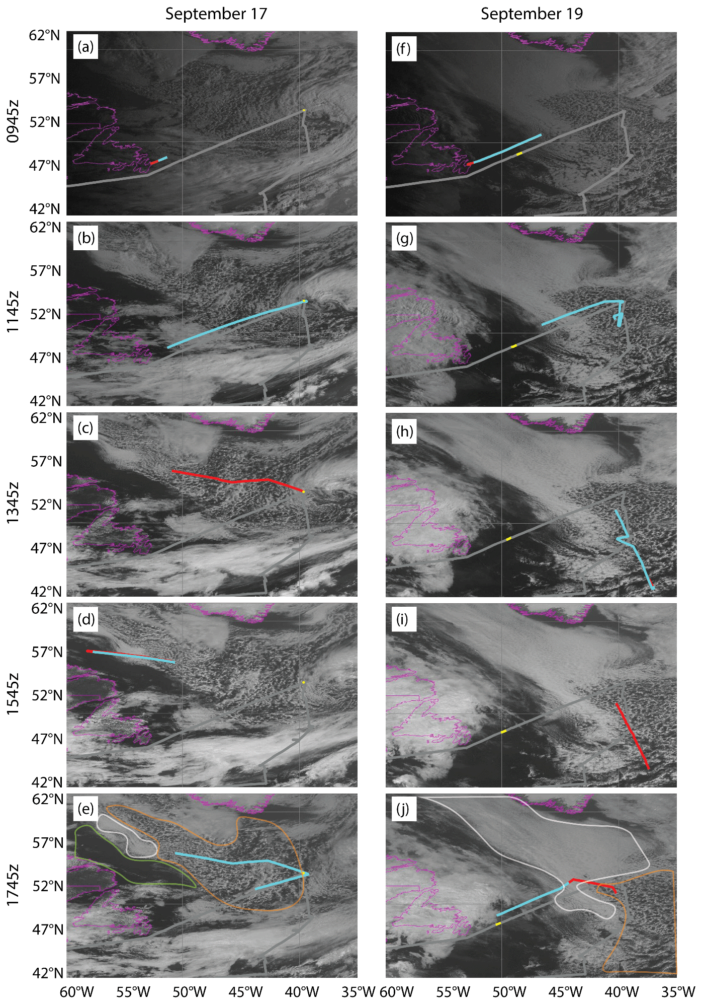
Figure 1GOES-East visible satellite imagery at 2 h intervals for 17 September 2017 (a–e) and 19 September 2017 (f–j). Purple lines outline the coast of eastern Canada and the southern tip of Greenland. Cyan and red lines represent the flight track at altitudes >3 km and <3 km, respectively, ±1 h from the satellite image time (shown on the y axis). The yellow line represents the ship position ±1 h from the satellite image time. The gray line is the entire ship track for the NAAMES3 campaign. (e, f) The cloud-free, closed-cell, and open-cell regions of interest are shown with approximate outlines in green, white, and orange, respectively.
This study focuses on aerosol and cloud measurements in and around a cold-air outbreak event that occurred over the western North Atlantic Ocean on 17–19 September 2017 (depicted by the GOES visible imagery shown in Fig. 1). The NAAMES3 campaign ship cruise track is given by the thick, gray line and instantaneous ship (yellow points) and aircraft positions (red lines when altitude <3 km and cyan lines when altitude >3 km), coincident with each satellite image (±1 h), in Fig. 1. The large-scale wind direction of the cold-air outbreak tended to be northwesterly, which is consistent with the observed southeastward transition from closed- to open-cell clouds and advection of Arctic air down the Labrador Sea to the North Atlantic region. Aerosol measurements were collected on the R/V Atlantis as it transected the open-cell region of the cold-air outbreak (Figs. 1d, e, S1) and then passed under an adjacent mostly clear-sky region to the southwest (Figs. 1f–j, S1). Two complementary C130 flights were conducted on 17 and 19 September (from here on referred to as FLT17 and FLT19), where the FLT17 flight track was likely upwind of both the R/V Atlantis and the FLT19 flight track, as shown by FLEXPART trajectories, discussed in Sect. 3.5. During FLT17, the R/V Atlantis was positioned at a single measurement station for conducting over the side operations before voyaging southwest at 18:15 UTC on 17 September 2017. During FLT19, the ship was underway with a southwest heading.
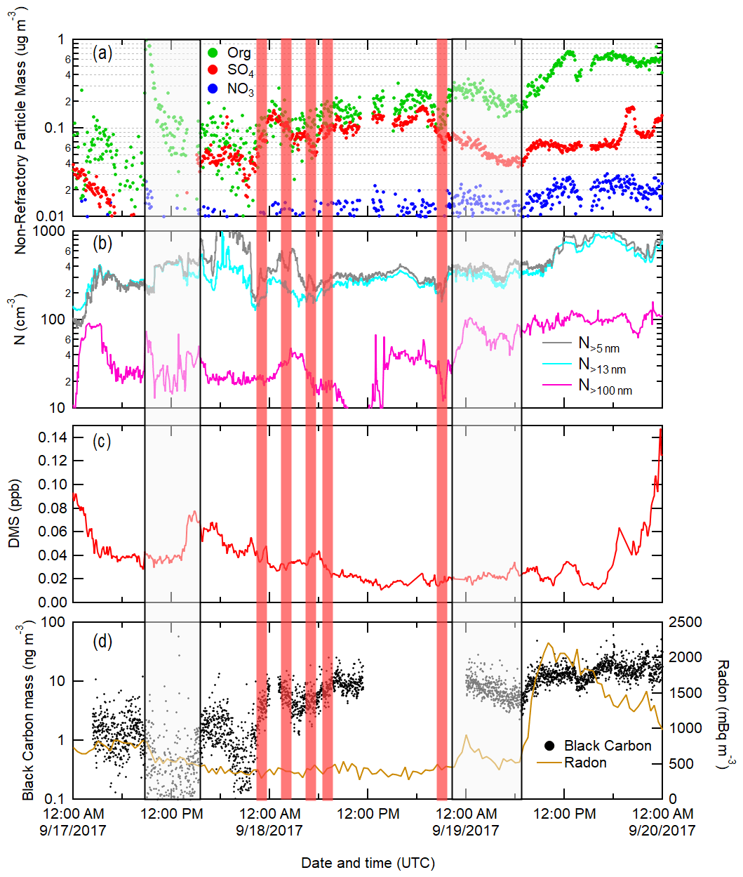
Figure 2The R/V Atlantis time series of (a) AMS organic, sulfate, and nitrate non-refractory particle mass shown as green, red, and blue points, respectively; (b) particle concentrations greater than 5, 13, and 100 nm shown as gray, cyan, and magenta lines, respectively; (c) DMS concentration; and (d) SP2 black carbon and radon concentration shown as black points and a brown line, respectively, over the time frame shown in Fig. 1. Particle concentrations >100 nm are measured with an scanning mobility particle sizer (SMPS) with the exception of a ∼1 d period (18 September) in which the SMPS was not operational. For this period, the DMPS measurements are shown. Black carbon measurements are not available for a ∼12 h period on 18 September when the SP2 was not operational. The two opaque boxed areas represent approximate periods in which air mass transitions occurred. The first transition (17 September, 08:00–16:00 UTC) was a result of the passing of an occluded front with a region of open-cell clouds following (Fig. 1a–e), and the second transition (22:00 UTC on 18 September–07:00 UTC on 19 September) is a result of the ship entering a polluted air region. The red vertical lines mark the 1 h period of measurements used in Table 3 comparisons.
3.1 Summary of R/V Atlantis and C-130 observations
The time series of the R/V Atlantis particle and DMS concentrations as well as particle composition from 17 through 19 September 2017 is shown in Fig. 2, where the two highlighted boxes emphasize the transitions in measured aerosol regimes. The first transition is due to the passing of an occluded front with a region of open-cell clouds following behind, as seen by GOES images in Fig. 1a–e. The second transition involves the ship entering a region influenced by continental air, as evident from the elevated radon concentrations (>500 mBq m−3) (Fig. 2d). Between these two transitions the ship remains in the system of open-cell clouds (Figs. 1a–e, S1). In this open-cell region, the particle mass concentration increases as the R/V Atlantis travels southwest.
The aircraft measurements from FLT17 are conducted during 10:25–20:35 UTC on 17 September, upwind of the ship and FLT19 measurements conducted hours to days later, as discussed in detail in Sect. 3.3. The black carbon concentration on both flights is consistent with previously identified clean marine conditions (<25 ng m−3) (Saliba et al., 2020; Sanchez et al., 2021), and similarly the observed carbon monoxide is consistent with observations made at an eastern North Atlantic research facility that is dominated by clean marine conditions (<130 ppb) (Zheng et al., 2018) for near-surface measurements made on both flights (Figs. S2 and S3). Carbon monoxide has a lifetime of about 1 month (Seinfeld and Pandis, 2006) and, therefore, is normally elevated in the North Atlantic relative to polar regions and other remote ocean regions that are not as often directly upwind of continental regions.
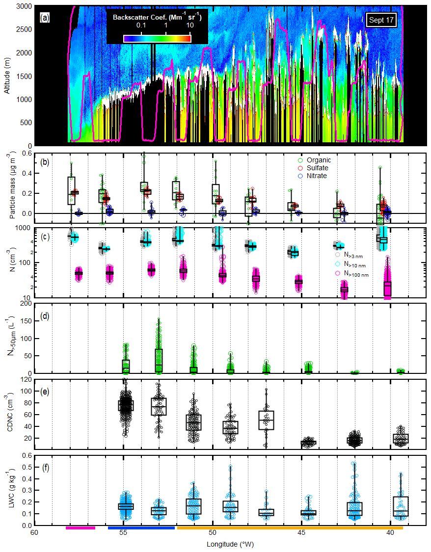
Figure 3C130 particle measurements collected on the 17 September 2017 flight. The (a) C130 HSRL backscatter overlaid with C130 altitude (magenta), (b) non-refractory particle mass composition, and (c) particle concentrations (N) for particles >3, >10, and > 100 nm in diameter. In-cloud (d) precipitation from the CIP (diameter >50 µm) and (e) CDNC (diameter range of 2–50 µm) and (f) LWC from the CDP are shown with box plots for each in-cloud leg. All measurements are presented as a function of longitude. The high-altitude HSRL back scattering measurements were made immediately after the surface measurements along the same horizontal flight track but in reverse (Fig. 1c–e). Magenta, blue and orange lines, at the bottom of panel (f), represent the approximate longitudes with cloud-free, closed-cell and open-cell clouds, respectively. Note that while negative particle mass measurements are not possible, they are included to prevent exclusion of the negative bias in the AMS measurements.
3.2 17 September 2017 flight (FLT17)
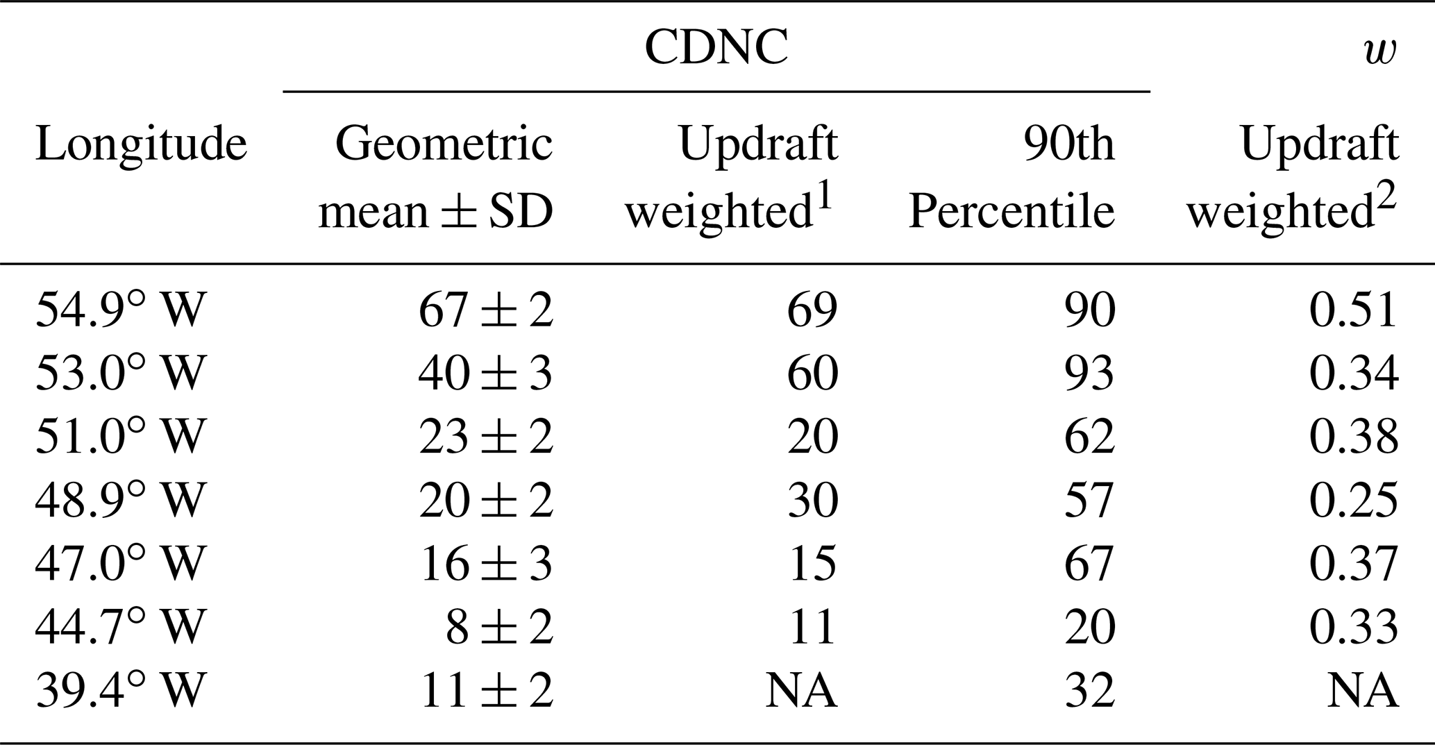
Figure 3 shows C130 marine boundary layer particle, cloud droplet number concentration (CDNC), and HSRL backscatter coefficient as a function of longitude for the roughly east–west flight paths shown in Fig. 1c–e. After arriving at the ship, the aircraft initially transited west at low altitude making in situ measurements before spiraling up to high altitude near 57∘ W and retracing the same flight path with the HSRL. Because the aircraft was continually ascending and descending throughout the marine boundary layer during the in situ sampling flight portion, we group the data into statistical boxes that represent the near-surface horizontal clear air legs (∼0.1 km altitude) for the aerosol shown in Fig. 3b and c. Similarly, the cloud measurements (Fig. 3d–f) are grouped for each in-cloud horizontal leg (∼1.0–1.5 km altitude) and also the vertical profile at ∼39.5∘ W. The nature of collecting CDNC along a linear flight path can introduce a bias if measurements are disproportionately collected on cloud edges (downdraft regions) or cloud cores (updraft regions). For this reason, Table 1 includes several summary CDNC and updraft velocity statistics for each cloud leg. The CDNC geometric mean limits the influence of outliers relative to a simple arithmetic mean, while the updraft weighted CDNC removes the inclusion of measurements in downdrafts where CDNC may be decreasing due to evaporation, and, finally, the 90th percentile likely represents an approximate value of the CDNC in an adiabatic updraft core. The weighted updraft is also included to show that the change in CDNC is not simply due to a change in updraft velocity. For example, the weighted updraft velocity at 53.0 and 44.7∘ W is 0.34 and 0.33 m s−1, respectively, but the CDNCs between the two locations vary by a factor of 3–5. Figure 3a shows the C130 altitude from the low-altitude aircraft flight track overlaid on the high-altitude remote HSRL backscatter curtain over the same flight track, which was obtained during a high-altitude, remote sensing leg that was conducted immediately after the near-surface in situ measurement flight legs with minimal delay. It is apparent from Fig. 3e that the westernmost two in-cloud legs (at 53 and 55∘ W) tended to have average CDNCs that were approximately 2–4 times higher than those observed on the eastern part of the track. The CIP measurements in Fig. 3d show that the clouds were precipitating, with peak precipitation sized droplets near the open-to-closed-cell transition, indicating there was removal of aerosol and cloud droplets through precipitation scavenging. This is consistent with previously published observations (Abel et al., 2017; Mechoso et al., 2014; Wood et al., 2011) and simulations (Mechoso et al., 2014; Wang and Feingold, 2009; Yamaguchi et al., 2017), showing reductions in CDNC ranging from 50 % to 90 %. These two regimes are identifiable in both the GOES imagery (Fig. 1), as well as the HSRL curtain (Fig. 3a), where the highest observed CDNCs are in the closed-cell cloud regime to the west, while the lowest CDNCs are in the open-cell cloud regime to the east. Intermediate CDNCs are apparent in the transitional region in between. While the overall aerosol number concentration (N>3 nm) does not have a clear trend throughout this period, the accumulation mode aerosol number concentration (N>100 nm) (Fig. 3c) and bulk organic and sulfate particle mass concentration (Fig. 3b) are lower on the eastern part of the flight, consistent with the lower CDNCs. There is no clear trend in the observed LWC (Fig. 3f), other than the fact that the highest LWCs were higher in the open-cell region, where cloud tops were higher. The HSRL particle backscatter coefficient measurements show the westernmost near-surface horizontal leg occurred in a cloud-free zone west of the closed-cell cloud regime (Fig. 3a). Notably, the observed near-surface particle concentrations and the back trajectories initialized in the cloud-free and closed-cell regimes are similar (53–59∘ W in Figs. 3b, c, S4), demonstrating that both regimes contain similar particle populations and have a similar source, despite differences in cloud coverage.
Table 1In-cloud leg measurements of CDNC (cm−3) and updraft velocity (w, m s−1) from the C130 flight on 17 September 2017 (Fig. 3). Cases when updraft measurements are not available for calculations are indicated in the table as NA.
.
.
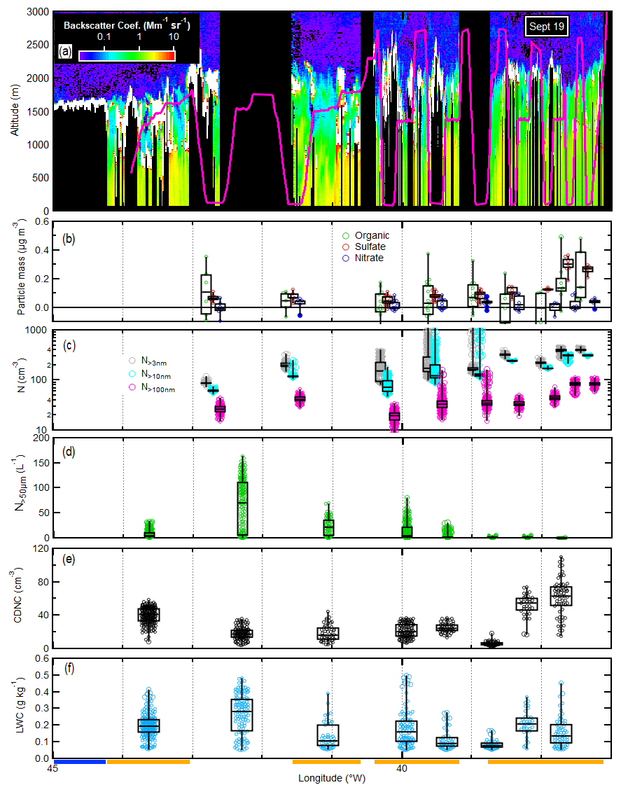
Figure 4C130 particle measurements collected on the 19 September 2017 flight. The (a) C130 HSRL backscatter overlaid with C130 altitude (magenta), (b) non-refractory particle mass composition, and (c) particle concentrations (N) for particles >3 nm, >10, and >100 nm in diameter. In-cloud (d) precipitation from the CIP (diameter >50 µm) and (e) CDNC (diameter range of 2–50 µm) and (f) LWC from the CDP are shown with box plots for each in-cloud leg. All measurements are presented as a function of longitude. The high-altitude HSRL back scattering measurements were made immediately before the surface measurements along almost the same horizontal flight track but in reverse (Fig. 1g–j). Any detours made at high latitude from the horizontal surface flight path were excluded from the HSRL swath shown. Blue and orange lines, at the bottom of panel (f), represent the approximate longitudes with closed-cell and open-cell clouds, respectively. Note that while negative particle mass measurements are not possible, they are included to prevent exclusion of the negative bias in the AMS measurements.
3.3 19 September 2017 flight (FLT19)
Figure 4 shows C130 marine boundary layer aerosol, cloud droplet measurements, and HSRL back scatter coefficient as a function of longitude (similar to the FLT17 case in Fig. 3) for the flight paths shown in Fig. 1g–j. Similar to Table 1, Table 2 includes CDNC and updraft velocity statistics for each cloud leg, showing the trend along the flight path. Note the portion of FLT19 shown in Fig. 1i has a significantly larger northward component compared to the low-altitude portion of the flight path shown in Fig. 1j, causing the higher density of vertical profiles and horizontal leg measurements between 37 and 40∘ W in Fig. 4 and Table 2. Figure 1 satellite images and Fig. 4a HSRL backscatter measurements show that none of the near-surface or in-cloud measurements were in the closed-cell region of the cold-air outbreak. Similar to the FLT17 case, the HSRL curtain covered roughly the same horizontal location as the C130 surface measurements in Fig. 4 (data are not reported here for two periods where the aircraft deviated from the subsequent low-altitude flight track). For FLT19, the high-altitude remote sensing leg was conducted immediately before the in situ surface measurements. A key feature to note in Fig. 4 is the significant change in average particle concentration and CDNC to the west of 40∘ W. Also, the clouds associated with the high particle and CDNC are non-precipitating (Fig. 4d). Further analysis in Sect. 3.3.2 suggests that the higher particle and CDNC region is downwind of the cloud-free region measured on FLT17 and not the cold-air outbreak. In the remaining sections, we explore the cause of the differing adjacent meteorological conditions and their impact on downwind aerosol and cloud properties.
Table 2In-cloud leg measurements of CDNC (cm−3) and updraft velocity (w, m s−1) from the C130 flight on 19 September 2017 (Fig. 4).
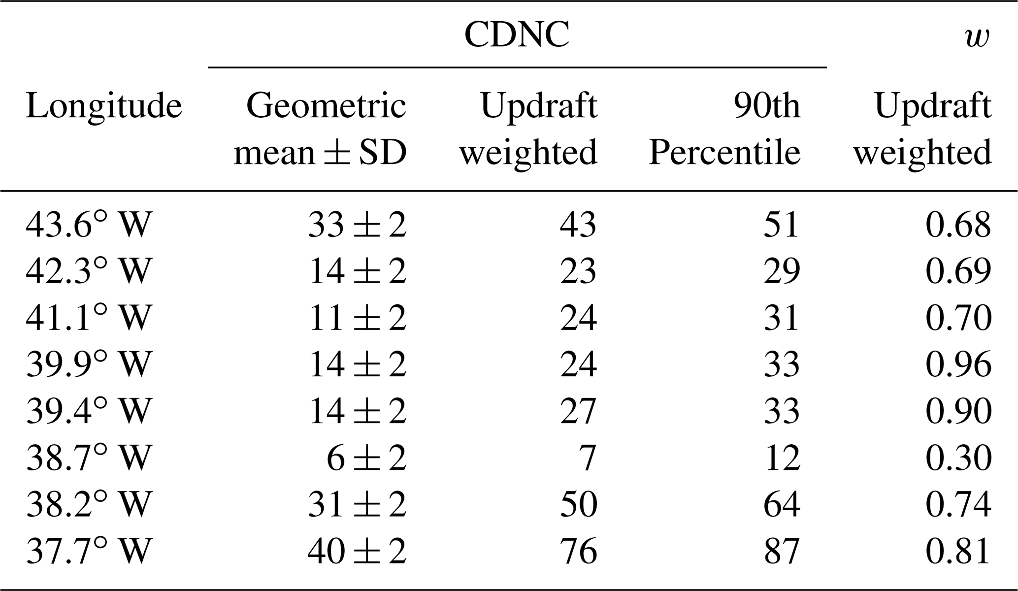
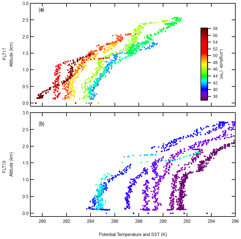
Figure 5Vertical profiles of the potential temperature from C130 flights that occurred on (a) 17 September 2019 and (b) 19 September 2019 (Figs. 3a and 4a). In-cloud measurements are excluded. Vertical profiles with horizontal in-cloud legs are excluded as well as a few others that have significant overlap with the presented vertical profiles. Surface measurements (at 0 km) represent the SST just below the lowest point in the vertical profile. The point color represents the longitude at which the measurement was made. Air mass transitions from open-cell to closed-cell clouds and from closed-cell to cloud-free air on the 17 September 2019 flight occurred at approximately 52 and 56∘ W, respectively. None of the vertical profiles are in the closed-cell region for the 19 September 2019 flight.
3.4 C130 vertical profile stability
Figure 5a and b present vertical profiles of potential temperature corresponding to the aircraft inline ascents and descents shown in Fig. 3a and Fig. 4a for FLT17 and FLT19, respectively. Only continuous vertical profiles are included in Fig. 5, though some are excluded to prevent substantial overlap of multiple similar vertical profiles. The square points at the sea surface (0 km altitude) represent the satellite-measured SST. The color of each point in Fig. 5 represents the longitude at which the measurement was made. For FLT17, shown in Fig. 5a, the marine boundary layer is neutrally buoyant to the west and becomes increasingly decoupled farther to the east (with the exception of the western most vertical profile at 58∘ W). This evolution in the profile stability and particle concentration is consistent with cold-air outbreaks where processes in the closed-cell region cause the marine boundary layer to decouple, leading to the transition from closed- to open-cell clouds (Abel et al., 2017; Albrecht et al., 1995; Christensen et al., 2020; de Roode et al., 2016; Sandu and Stevens, 2011; Wood et al., 2011; Yamaguchi et al., 2017). None of the vertical profiles from FLT19 are in the closed-cell region, but the profiles to the west, nearest the closed-to-open-cell transition of the cold-air outbreak, are decoupled and stable (Fig. 5b), consistent with observations in FLT17. However, the neutrally buoyant boundary layers to the east of 40∘ W are not consistent with this pattern. These boundary layer profiles are neutrally stable, despite being in an area of cumulus clouds because the eastern portion of the flight is not actually part of the open-cell region of cold-air outbreak or even downwind of it (discussed in Sect. 3.3.2) and is therefore not influenced by meteorological processes associated with the cold-air outbreak.
Table 3The absolute and relative difference in aerosol between the downwind and upwind measurements for the cases in which 2 d FLEXPART back trajectories initialized by the R/V Atlantis or C130 location overlap with upwind C130 measurement locations (within 1∘ latitude and longitude and 3 h), shown in Figs. 6 and 7. The number of hours between the upwind and downwind measurements (Δt) are also included. R/V Atlantis measurements are derived from a 1 h average. The difference in absolute values of the particle composition and concentration is calculated as an average ±1 SD. Values in bold indicate upwind and downwind measurement distributions are significantly different, assuming confidence interval of >99 %. The number of measurements used for each comparison, provided in Table S1, vary depending on sampling time and platform.
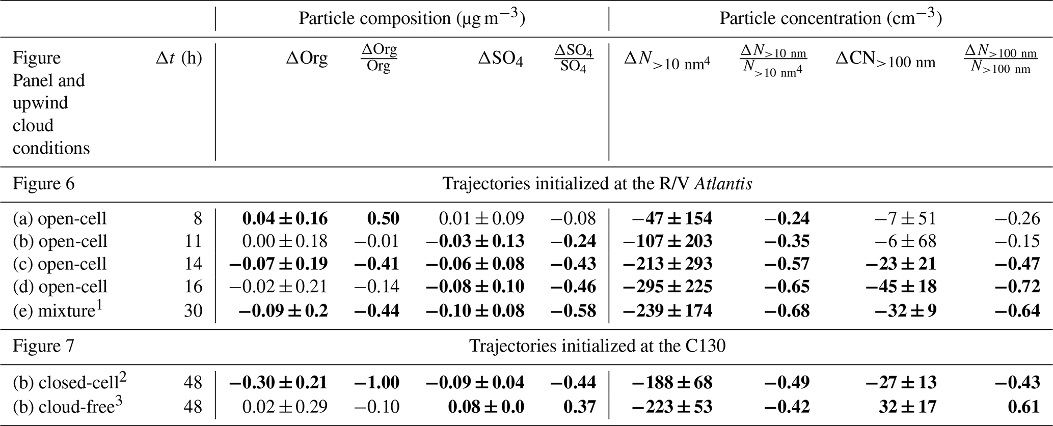
1 Upwind measurements are near the transition between cloud-free and closed-cell regions, and, therefore, downwind measurements possibly represent a mixture of the two regimes. 2 Difference between the measurements in the FLT17 closed-cell region and FLT19 low-particle-concentration region. Specifically, FLT17 measurements in the closed-cell region at 53.5∘ W (Figs. 3, 7b) are compared to downwind FLT19 C130 surface measurements between 37.8–38.5∘ W (Figs. 4, 7b). 3 Difference between the measurements in the FLT17 cloud-free region and FLT19 high-particle-concentration region. Specifically, FLT17 measurements in the cloud-free region at 57.8∘ W (Figs. 3, 7b) are compared to downwind FLT19 C130 surface measurements east of 37.8∘ W (Figs. 4, 7b). 4 R/V Atlantis N>13 nm measurements are used for comparison to C130 N>10 nm measurements.
The FLT17 stable vertical profile at about 58∘ W (Fig. 5a) is from the clear-sky region that is to the west of the closed-cell region (Fig. 1d). This vertical profile is very stable and strongly decoupled. The cause of the differing atmospheric stability in this region is the low SST (Fig. 5a), which cools and stabilizes the marine boundary layer, preventing the vertical transport of water vapor and cloud formation. For almost all the other vertical profiles in Fig. 5, the SST is greater than the atmospheric temperature near the sea surface, consistent with the processes of advection of cold air over warm SST that lead to the stratocumulus-to-cumulus transitions in cold-air outbreaks (Albrecht et al., 1995; de Roode et al., 2016). The neutrally stable vertical profiles with higher particle concentrations and CDNC in FLT19 (Figs. 5b and 4b, c, e) are actually downwind of this same clear-sky region (further discussed in Sect. 3.3.2). The reason for the characteristic differences in the measurements downwind of the clear-sky and cold-air outbreak regions, despite their initial close proximity, is discussed in the following section examining relevant FLEXPART back trajectories.
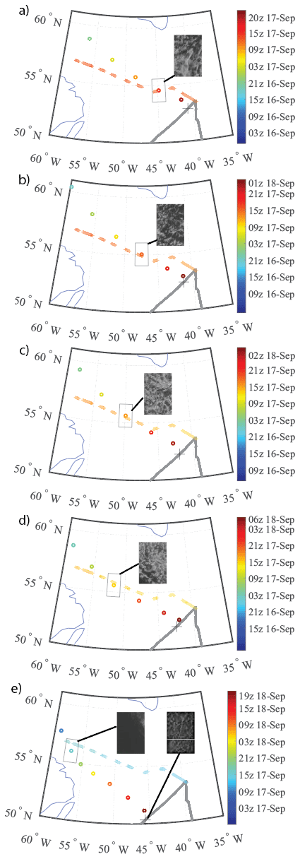
Figure 6The location of FLEXPART back trajectories averaged over 6 h intervals (shown as open circles) and low-level (∼0.1 km) C130 surface measurements (shown as colored lines) are both colored as a function of time. The color bar range is different for each panel and is defined by the initialization time and end time of a 2 d FLEXPART back trajectory initiated at the R/V Atlantis. The initialization times for the back trajectories are (a) 23:00 UTC on 17 September, (b) 02:00 UTC on 18 September, (c) 05:00 UTC on 18 September, (d) 07:00 UTC on 18 September, and (e) 21:00 UTC on 18 September. The gray line represents the R/V Atlantis ship track, and the black cross on the ship track in panels (a)–(e) represents the location of the R/V Atlantis for the initialized back trajectory. The black rectangles around individual FLEXPART back trajectory intervals show the area in which C130 measurements were averaged and compared to downwind particle measurements (Table 3). The GOES-East satellite visible image for the area is included to present the cloud coverage corresponding to the time of the averaged 6 h back trajectory interval. The GOES-East visible satellite image of the area around the ship initialization point in panel (e) is also included. Other trajectories were initialized at night and have no corresponding visible image.
3.5 Particle evolution along FLEXPART trajectories
3.5.1 FLT17 to R/V Atlantis trajectories
The R/V Atlantis ship track was well placed downwind of the portion of FLT17 shown in Fig. 1c–d such that spatially averaged FLEXPART back trajectories initialized from the ship position overlap in time and space (within 3 h and 1∘ latitude and longitude) with the C130 near-surface measurements (Fig. 6). This overlap enabled the comparison of measured particle properties between the C130 and R/V Atlantis to identify changes over time. In Fig. 6, available (daylight only) visible GOES images of the area are shown and aligned with the 6-hourly trajectory interval that overlaps the upwind FLT17 measurements or at the initialization location of the back trajectory. These images are shown to identify if measurements were made in the cloud-free, open- or closed-cell regions. Upwind, near-surface C130 measurements within 1∘ latitude and longitude and 3 h of the back trajectory point are averaged and subtracted from the downwind ship measurements (shown in Table 3) to represent changes in the particle properties during transport. In general, both particle mass and number concentration decreased over the trajectory. However, the difference in particle concentrations is less than the standard deviation for some cases and therefore within the measured variability. This occurs mostly when the trajectory length is short, and therefore changes in particle properties over the short time period are minimal. Also, particle number concentrations have somewhat smaller standard deviations than particle mass concentrations, due to the greater sampling rate and smaller instrument error of the CPC and LAS, compared to the AMS. The time periods used for the R/V Atlantis measurements in this comparison are from 10 min averages at the back trajectory initialization time (highlighted in Fig. 2). The magnitude of the decrease in particle number concentration generally increased for the longer trajectory times (8–16 h) with the exception of the last trajectory (shown in Fig. 6e). This last trajectory is different in that its path is near the transition between the cloud-free and closed-cell regions (Figs. 1d, 6e). The satellite image at the R/V Atlantis location (the trajectory initialization location) shows open-cell clouds, which could mean clouds had formed along the trajectory or that the measurement is some combination of both air from the cloud-free region and the closed-cell region upwind. Either way, the different meteorological processes in the initially cloud-free and closed-cell region of the cold-air outbreak likely resulted in the overall rate of particle removal between the two measurements relative to upwind trajectories that were clearly in the cold-air outbreak (Table 3).
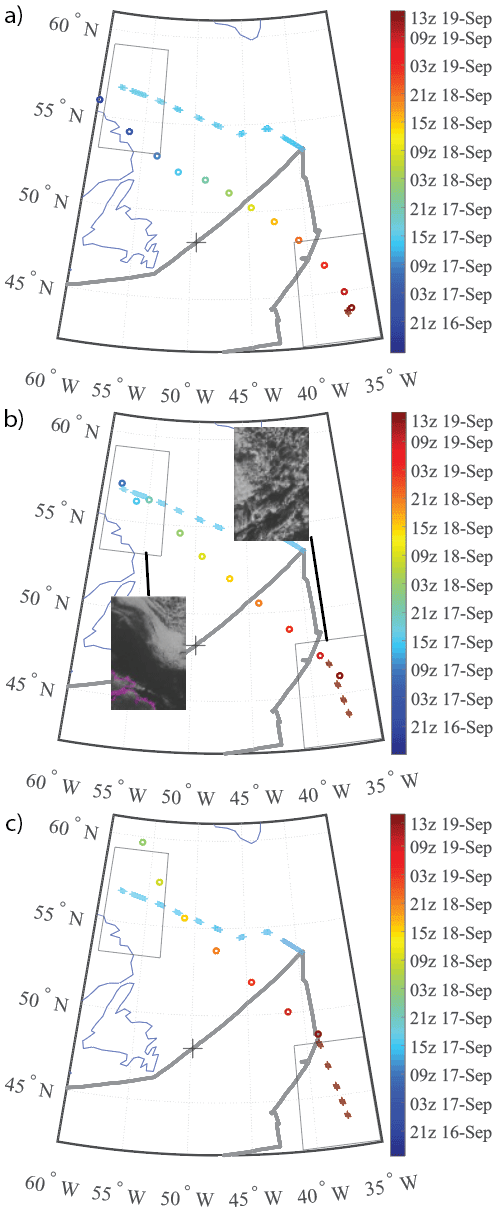
Figure 7The location of FLEXPART back trajectories averaged over 6 h intervals (shown as open circles) and low-level (∼0.1 km) C130 surface measurements (shown as colored lines) are both colored as a function of time. The color bar range shifts by 40 min in each panel and is defined by the start and end of a 3 d FLEXPART back trajectory initiated at the C130 horizontal location at 500 m above the sea surface. The initialization times for the back trajectories are (a) 14:24 UTC on 19 September, (b) 15:04 UTC on 19 September, and (c) 15:44 UTC on 19 September. The gray line represents the R/V Atlantis ship track, and the black cross on the ship track in panels (a)–(c) represents the location of the R/V Atlantis for the initialized back trajectory. The black boxed area that overlaps the trajectory (b) and FLT17 surface measurements identifies the C130 measurements used for comparison with downwind C130 measurements from FLT19 shown by the second area. GOES-East visible images are shown in panel (b) for both areas corresponding to the back trajectory initialization time and the 48 h back trajectory interval that overlaps with FLT17 near-surface measurements. Table 3 contains comparisons between measurements made on FLT19 and measurements from the closed-cell and cloud-free region upwind from FLT17.
3.5.2 FLT17 to FLT19 trajectories
FLEXPART back trajectories are also initialized with FLT19 near-surface measurements, which are downwind of the FLT17 flight path. The initial easternmost aerosol measurements from FLT19 (Figs. 1i, 4b–e) have the highest aerosol mass and number concentrations, as well as CDNC, for the low-level in situ measurements shown in Fig. 4. Examining the FLEXPART back trajectories initialized at this location, we find the upwind source of the region with high particle concentrations transported from the cloud-free stable boundary layer observed in FLT17. Figure 7 highlights this shift in the upwind source with trajectories that cross the cloud-free region (Fig. 7a), the transition zone between the closed-cell and cloud-free regions (Fig. 7b), and the closed-cell region of the cold-air outbreak (Fig. 7c). Since the Fig. 7b trajectory aligns the transition zone between the closed-cell and cloud-free region upwind and the transition zone between low and high particle concentrations downwind, this trajectory is used to compare both pairs of measurements on either side of these zones. Table 3 shows calculations of the difference in downwind (FLT19) and upwind (FLT17) observed particle loadings, which we use to infer differences in particle evolution from the cloud-free region leading up to the observed FLT19 high particle concentrations and the evolution of particles from the closed-cell region to the observed FLT19 low particle concentrations. Over approximately 48 h, particles that advected from the closed-cell region of the cold-air outbreak in FLT17 to the open-cell region between 37.8 and 38.5∘ W in FLT19 show the average organic and sulfate concentrations significantly decreased (100 % and 44 %, respectively) in the cold-air outbreak (Table 3). The preferential removal of organic mass is unexpected as sulfate is more hygroscopic and therefore more likely to activate to form cloud droplets and be lost through precipitation processes. It is possible the sulfate mass resided in smaller particles that are less likely to form cloud droplets or that there are differences in the replenishment of mass via marine or entrained sources, similar to previous particle formation events observed in cloudy marine environments (Clarke et al., 1999; Hegg et al., 1990; Perry and Hobbs, 1994; Sanchez et al., 2018). Vertical profiles of CN>10 nm (Fig. S5a), corresponding to the potential temperature profiles in Fig. 5, mostly show lower particle concentrations above 1–1.5 km (the range of boundary layer heights based on Fig. 5) relative to the surface, suggesting it is likely not a net source of particles in this case. Also, the decoupling of the boundary layer acts as a buffer, inhibiting the transfer of particles and gaseous precursors between the surface and lower free troposphere. Sanchez et al. (2021) showed that organic aerosol mass is moderately correlated with in-water biological activity, while sulfate aerosol mass is only weakly correlated. They attributed the difference to the relatively short lifetime of the organic aerosol precursors like isoprene and monoterpenes (minutes to hours) versus sulfate precursors like DMS (>1–2 d). We speculate that the various source strength and precursor residence time may play a role in the resulting shift in the organic-to-sulfate mass ratio. Additionally, the CN>10 nm and CN>100 nm particle concentrations both decreased by 40 %–50 % (Table 3). Conversely, over the same approximate 48 h period, particles that advected from the cloud-free region in FLT17 to the cumulus cloud region east of 37.8∘ W in FLT19 show a decrease in organic particle concentration within the observed variability (10 %) and an increase in sulfate particle concentration (37 %) (Table 3). The CN>10 nm and CN>100 nm particle concentrations decreased by 42 % and increased by 62 %, respectively (Table 3). The upwind vertical profile of CN>10 nm on FLT17 in Fig. S5a shows there was a strong negative gradient with altitude in the cloud-free region (at ∼58∘ W), suggesting the decrease in the observed surface CN>10 nm between FLT17 and FLT19 is likely due to dilution when mixing with lower concentrations higher in the boundary layer upon destabilization of the boundary layer. Also, the reduction in stability likely enhanced entrainment with the lower free troposphere, which is shown to have relatively high particle concentrations in the 19 September case (Fig. S5b). The formation of sulfate particles due to mixing between the marine boundary layer and lower free troposphere is supported by another NAAMES study (Sanchez et al., 2018) and others (Clarke et al., 1999; Dzepina et al., 2015; Moore et al., 2003) and likely explains at least part of the increase in sulfate particle mass along this trajectory. The in-cloud CIP measurements from FLT19 (Fig. 4d, in the region downwind of the cloud–free region, east of 37.8∘ W) show essentially no precipitation size droplets; however, we cannot rule out precipitation occurring along the trajectory between the FLT17 cloud-free region and downwind FLT19 measurements. The differences in the meteorology along these trajectories suggests that the trajectory outside the cold-air outbreak likely had less precipitation and corresponding collision–coalescence scavenging, resulting in the observed differences in the particle property evolution.

Figure 8September 2017 averaged satellite (a) SST and (b) CF. (c) The pixel-by-pixel comparison of SST and CF from the boxed area in panels (a) and (b). (d) The Pearson coefficient for the pixel-by-pixel linear regression comparing SST and CF for the boxed area (shown in panels a and b) for every month from August 2008–June 2019. Correlations with P>0.05 have been excluded.
3.6 Ocean SST control of atmospheric stability
Averaged satellite SST measurements for September 2017 (corresponding to the NAAMES3 mission) show a local minimum in SST (highlighted by the black box in Fig. 8a) in the cloud-free region to the west of the observed closed-cell region in FLT17 (Fig. 1c). The southerly flow of the Labrador Current bringing cold water from the Arctic Ocean (Fig. S6) causes the observed minimum in SST. Figure 8b shows the spatially collocated minimum in the average cloud fraction (CF), consistent with the visible satellite images in Fig. 1. Figure 8c shows the linear regression between the September 2017 averaged SST and CF from the boxed areas in Fig. 8a and b. Each point in Fig. 8c represents a pixel-by-pixel comparison from the boxed region of Fig. 8a and b. The spatial correlation between the SST and CF suggests that the SST strongly influences the CF in this region during NAAMES3, likely because the air at the surface cools and stabilizes the atmospheric marine boundary layer (consistent with the stable vertical profile and SST at 58∘ W shown in Fig. 5a). A stable marine boundary layer prevents vertical transport of water vapor, thus trapping moisture near the surface, inhibiting cloud formation in the region, and producing the persistent low CF relative to the surrounding area. Our Lagrangian analysis in Sect. 3.3 demonstrates the significant difference in meteorological impacts on cloud properties and particle concentrations downwind of this very stable boundary layer and the adjacent closed-cell region of a cold-air outbreak.
To identify how consistently the SST influences the CF and meteorology in this region, CF and SST are compared for each month using satellite observations from August 2008 to June 2019. The correlation (Pearson's coefficient) between the CF and SST is consistently highest in the late summer, peaking in September, consistent with NAAMES3 analyzed case studies (Fig. 8d). Even the wind direction from MERRA-2, over the same ∼11-year time period, is typically from the northwest (Fig. S7), parallel to the Labrador Current, which is necessary for measurements in the North Atlantic to be downstream of the highlighted area of interest in Fig. 8. Based on these results and the Lagrangian cases shown, this region is an ideal location to study the effect of cloud processing on marine boundary layer particle properties. The proximity of the cloud-free and cold-air outbreak closed-cell region is close and therefore likely often containing inflows of air from similar sources, with similar particle properties. In addition, the difference in meteorological conditions caused by the SST pattern in the region enables one to compare the evolution of the particles initialized in these two different meteorological regimes over a Lagrangian trajectory. The controlling SST forcing on cloud formation in this region of study suggests changes in North Atlantic cold-air outbreaks, due to changes in climate, could have major implications for cloud and particle properties in the North Atlantic. In a previous modeling study Kolstad and Bracegirdle (2008) have shown cold-air outbreaks in the North Atlantic are predicted to weaken in the late 21st century as the difference in the atmospheric temperature and SST is expected to decrease and therefore will likely affect the influence cold-air outbreaks have on the evolution of cloud and aerosol properties.
Here, we examine the evolution of atmospheric aerosols and clouds along adjacent Lagrangian air mass trajectories over the North Atlantic during a cold-air outbreak event in 2017. While particle number concentrations and mass composition are similar within the northwest (i.e., upwind) portion of the study region, the cloud conditions are very different, with a notable clear air region above the Labrador Current, driven by cool sea surface temperatures stabilizing the marine boundary layer and a stratiform cloud and less stable region immediately to the northeast over warmer waters. This clear-to-cloudy transition is well captured by the NASA C-130 and HSRL measurements from NAAMES, which confirmed the similar aerosol conditions across the transition region. Subsequent measurements downwind of these regions, which we connect back using FLEXPART model trajectories, show that the aerosol fields evolve very differently depending on whether they started out in the clear or cloudy areas.
Along the trajectory just outside of the cold-air outbreak, where the initial cloud-free air evolves to cumulus clouds, we observe no changes in the organic mass but an increases in sulfate mass (37 %) and large particle (diameter >100 nm) concentration (61 %) over a 48 h period (Table 3). We contrast this case with the adjacent trajectory that is inside the cold-air outbreak, where the closed-cell stratiform clouds evolve and become open-cell cumulus clouds. For this case, we observe large reductions in aerosol particle and cloud droplet number concentrations as well as an approximate 100 % depletion of the organic aerosol mass concentrations over the 48 h period (Table 3). Surprisingly, we observed only a 44 % reduction in sulfate aerosol mass over this same trajectory. For both cases, the change in the organic-to-sulfate mass ratio is unexpected as sulfate components are more hygroscopic and therefore more likely to activate to form cloud droplets and be removed through precipitation. Vertical profiles of CN suggest the free troposphere was a source of sulfate entrained into the marine boundary layer, especially for the profiles with less stable boundary layers, which would enhance vertical entrainment. It is also possible that the sulfate resided in smaller particles or more of the sulfate was removed through precipitation and subsequently more sulfate particles were formed via gas phase or in-cloud oxidation of SO2. Sanchez et al. (2021) showed that organic aerosol mass is moderately correlated with in-water biological activity, while sulfate aerosol mass is only weakly correlated. They attributed the difference to the relatively short lifetime of the organic aerosol precursors like isoprene and monoterpenes (minutes to hours) versus sulfate precursors like DMS (>1–2 d). Given the localized area of the higher ocean chlorophyll and biological activity to the northwest (Fig. S8), we speculate that while both organic and sulfate aerosol species are rapidly depleted by wet scavenging along the cold-air outbreak trajectory (i.e., the closed-to-open-cell transition), the sustained secondary sulfate source is able to replenish the sulfate aerosol concentration. Meanwhile, the organic aerosol does not recover over this period, which gives rise to the 100 % decrease in organic mass observed during NAAMES.
This case study is ideal for future model simulation because the dramatic gradient in SST caused by the Labrador Current essentially bifurcates the atmosphere along two pathways for aerosol–cloud evolution. This results in different initial cloud conditions (clear vs. closed-cell clouds), but similar initial aerosol conditions. Meanwhile, the downwind conditions are similar for the clouds (cumulus clouds), but the aerosol number and speciated mass concentrations are quite different. We speculate that these differences are driven by different amounts of cloud processing along the adjacent trajectories. C130 measurements of marine boundary layer potential temperature profiles are consistent with cloud-top entrainment and increased sea surface sensible and latent heating leading to the stabilization of the marine boundary layer. In addition, increased precipitation and collision–coalescence decreases the particle and cloud droplet concentrations. Both of these processes, in turn, lead to the transition from stratocumulus to convective cumulus clouds (Abel et al., 2017; Albrecht et al., 2016; Christensen et al., 2020; de Roode et al., 2016; Sandu and Stevens, 2011; Wood et al., 2011, 2017; Yamaguchi et al., 2017). The adjacent cloud-free and closed-cell regions appear to be driven by the sharp gradient in SST caused by the Labrador Current. To better understand how prevalent these conditions set up in this region, we analyzed 11 years of satellite measurements and found persistently low cloud fraction over the Labrador Current next to an area of high cloud fraction that occurs annually around September. This shows that future studies could take advantage of this reoccurring pattern to obtain more statistics and track the Lagrangian evolution of atmospheric aerosols resulting from different initial meteorological conditions.
The NAAMES dataset is archived at the NASA Atmospheric Science Data Center (ASDC; https://doi.org/10.5067/Suborbital/NAAMES/DATA001, last access: 30 January 2021, NAAMES Science Team, 2018) and the SeaWiFS Bio-Optical Archive and Storage System (SeaBASS; https://doi.org/10.5067/SeaBASS/NAAMES/DATA001, last access: 9 April 2020, Werdell and Bailey, 2002). Scripps measurements are available at https://doi.org/10.6075/J04T6GJ6 (last access: 9 April 2020, Russell et al., 2018). The GlobColour data (http://globcolour.info) used in this study have been developed, validated, and distributed by ACRI-ST, France (Maritorena et al., 2010; Fanton d'Andon et al., 2009). GDAS data (last access: 2 October 2019, DOC, 2020) are available at ftp://arlftp.arlhq.noaa.gov/pub/archives/gdas1/. No access credentials are required. The SST is acquired from the Global Australian Multi-Sensor Sea Surface Temperature Analysis (ABOM, 2008). OSCAR ocean currents are available at https://podaac-tools.jpl.nasa.gov/drive/files/allData/oscar/L4/oscar_1_deg (last access: 2 April 2021, ESR, 2007). MERRA-2 data are available through https://earthdata.nasa.gov (last access: 2 April 2021, Global Modeling And Assimilation Office, 2015).
The supplement related to this article is available online at: https://doi.org/10.5194/acp-22-2795-2022-supplement.
KJS and RHM were responsible for the visualization, conceptualization, methodology, and writing of the original draft. KJS and BZ designed the software. KJS performed the formal analysis. RHM and MHB were responsible for supervision, project administration, and funding acquisition. GS, SLL, MAS, LDZ, RHM, PKQ, TSB, JP, TGB, ESS, LMR, and MJB curated the data. All authors participated in writing, review, and editing.
At least one of the (co-)authors is a member of the editorial board of Atmospheric Chemistry and Physics. The peer-review process was guided by an independent editor, and the authors also have no other competing interests to declare.
Publisher’s note: Copernicus Publications remains neutral with regard to jurisdictional claims in published maps and institutional affiliations.
We thank the dedicated crew of the R/V Atlantis. Kevin J. Sanchez was funded by the NASA Postdoctoral Program. The authors also would like to acknowledge Raghu Betha, Derek Price, Derek Coffman, James Johnson, Armin Wisthaler, and Lucia Upchurch for collecting and reducing data. This is PMEL contribution number 5277. Bo Zhang and Hongyu Liu acknowledge the funding support from the NAAMES mission.
This research has been supported by the National Aeronautics and Space Administration (grant nos. NNX15AE66G, NNX15AF30G, and NNX15AF31G) and the Division of Ocean Sciences (grant no. NSFOCE-1537943).
This paper was edited by Joachim Curtius and reviewed by two anonymous referees.
Abel, S. J., Boutle, I. A., Waite, K., Fox, S., Brown, P. R. A., Cotton, R., Lloyd, G., Choularton, T. W., and Bower, K. N.: The role of precipitation in controlling the transition from stratocumulus to cumulus clouds in a Northern Hemisphere cold-air outbreak, J. Atmos. Sci., 74, 2293–2314, https://doi.org/10.1175/JAS-D-16-0362.1, 2017.
ABOM: GHRSST Level 4 GAMSSA Global Foundation Sea Surface Temperature Analysis, Ver. 1.0. PO.DAAC [data set], https://doi.org/10.5067/GHGAM-4FA01, (last access: 2 April 2021), 2008.
Ackerman, A. S., Toon, O. B., Taylor, J. P., Johnson, D. W., Hobbs, P. V., and Ferek, R. J.: Effects of aerosols on cloud albedo: Evaluation of Twomey's parameterization of cloud susceptibility using measurements of ship tracks, J. Atmos. Sci., 57, 2684–2695, https://doi.org/10.1175/1520-0469(2000)057< 2684:EOAOCA>2.0.CO;2, 2000.
Ackerman, A. S., Kirkpatrick, M. P., Stevens, D. E., and Toon, O. B.: The impact of humidity above stratiform clouds on indirect aerosol climate forcing, Nature, 432, 1014–1017, https://doi.org/10.1038/nature03174, 2004.
Albrecht, B. A.: Aerosols, cloud microphysics, and fractional cloudiness, Science, 245, 1227–1230, https://doi.org/10.1126/science.245.4923.1227, 1989.
Albrecht, B. A., Bretherton, C. S., Johnson, D., Schubert, W. H., and Frisch, A. S.: The Atlantic Stratocumulus Transition Experiment – ASTEX, B. Am. Meteorol. Soc., 76, 889–904, https://doi.org/10.1175/1520-0477(1995)076< 0889:TASTE>2.0.CO;2, 1995.
Albrecht, B. A., Fang, M., and Ghate, V.: Exploring stratocumulus cloud-top entrainment processes and parameterizations by using doppler cloud radar observations, J. Atmos. Sci., 73, 729–742, https://doi.org/10.1175/JAS-D-15-0147.1, 2016.
Andreae, M. O. and Crutzen, P. J.: Atmospheric aerosols: Biogeochemical sources and role in atmospheric chemistry, Science, 276, 1052–1058, https://doi.org/10.1126/science.276.5315.1052, 1997.
Ayers, G. P., Cainey, J. M., Gillett, R. W., and Ivey, J. P.: Atmospheric sulphur and cloud condensation nuclei in marine air in the Southern Hemisphere, Philos. T. Roy. Soc. B, 352, 203–211, https://doi.org/10.1098/rstb.1997.0015, 1997.
Balaguru, K., Doney, S. C., Bianucci, L., Rasch, P. J., Leung, L. R., Yoon, J. H., and Lima, I. D.: Linking deep convection and phytoplankton blooms in the northern Labrador Sea in a changing climate, PLoS One, 13, 1–17, https://doi.org/10.1371/journal.pone.0191509, 2018.
Bates, T. S., Huebert, B. J., Gras, J. L., Griffiths, F. B., and Durkee, P. A.: International Global Atmospheric Chemistry (IGAC) Project's First Aerosol Characterization Experiment (ACE 1): Overview, J. Geophys. Res.-Atmos., 103, 16297–16318, https://doi.org/10.1029/97JD03741, 1998a.
Bates, T. S., Kapustin, V. N., Quinn, P. K., Covert, D. S., Coffman, D. J., Mari, C., Durkee, P. A., De Bruyn, W. J., and Saltzman, E. S.: Processes controlling the distribution of aerosol particles in the lower marine boundary layer during the first aerosol characterization experiment (ACE 1), J. Geophys. Res.-Atmos., 103, 16369–16383, https://doi.org/10.1029/97JD03720, 1998b.
Behrenfeld, M. J. and Boss, E. S.: Student's tutorial on bloom hypotheses in the context of phytoplankton annual cycles, Glob. Chang. Biol., 24, 55–77, https://doi.org/10.1111/gcb.13858, 2018.
Behrenfeld, M. J., O'Malley, R. T., Boss, E. S., Westberry, T. K., Graff, J. R., Halsey, K. H., Milligan, A. J., Siegel, D. A., and Brown, M. B.: Revaluating ocean warming impacts on global phytoplankton, Nat. Clim. Chang., 6, 323–330, https://doi.org/10.1038/nclimate2838, 2016.
Behrenfeld, M. J., Moore, R. H., Hostetler, C. A., Graff, J., Gaube, P., Russell, L. M., Chen, G., Doney, S. C., Giovannoni, S., Liu, H., Proctor, C., Bolaños, L. M., Baetge, N., Davie-Martin, C., Westberry, T. K., Bates, T. S., Bell, T. G., Bidle, K. D., Boss, E. S., Brooks, S. D., Cairns, B., Carlson, C., Halsey, K., Harvey, E. L., Hu, C., Karp-Boss, L., Kleb, M., Menden-Deuer, S., Morison, F., Quinn, P. K., Scarino, A. J., Anderson, B., Chowdhary, J., Crosbie, E., Ferrare, R., Hair, J. W., Hu, Y., Janz, S., Redemann, J., Saltzman, E., Shook, M., Siegel, D. A., Wisthaler, A., Martin, M. Y., and Ziemba, L.: The North Atlantic Aerosol and Marine Ecosystem Study (NAAMES): Science motive and mission overview, Front. Mar. Sci., 6, 1–25, https://doi.org/10.3389/fmars.2019.00122, 2019.
Bell, T. G., De Bruyn, W., Miller, S. D., Ward, B., Christensen, K. H., and Saltzman, E. S.: Air–sea dimethylsulfide (DMS) gas transfer in the North Atlantic: evidence for limited interfacial gas exchange at high wind speed, Atmos. Chem. Phys., 13, 11073–11087, https://doi.org/10.5194/acp-13-11073-2013, 2013.
Bell, T. G., De Bruyn, W., Marandino, C. A., Miller, S. D., Law, C. S., Smith, M. J., and Saltzman, E. S.: Dimethylsulfide gas transfer coefficients from algal blooms in the Southern Ocean, Atmos. Chem. Phys., 15, 1783–1794, https://doi.org/10.5194/acp-15-1783-2015, 2015.
Bell, T. G., Porter, J. G., Wang, W. L., Lawler, M. J., Boss, E., Behrenfeld, M. J. and Saltzman, E. S.: Predictability of Seawater DMS During the North Atlantic Aerosol and Marine Ecosystem Study (NAAMES), Front. Mar. Sci., 7, 596763, https://doi.org/10.3389/fmars.2020.596763, 2021.
Berner, A. H., Bretherton, C. S., Wood, R., and Muhlbauer, A.: Marine boundary layer cloud regimes and POC formation in a CRM coupled to a bulk aerosol scheme, Atmos. Chem. Phys., 13, 12549–12572, https://doi.org/10.5194/acp-13-12549-2013, 2013.
Bonjean, F. and Lagerloef, G. S. E.: Diagnostic model and analysis of the surface currents in the Tropical Pacific Ocean, J. Phys. Oceanogr., 32, 2938–2954, https://doi.org/10.1175/1520-0485(2002)032< 2938:DMAAOT>2.0.CO;2, 2002.
Boss, E. and Behrenfeld, M.: In situ evaluation of the initiation of the North Atlantic phytoplankton bloom, Geophys. Res. Lett., 37, 1–5, https://doi.org/10.1029/2010GL044174, 2010.
Bretherton, C. S. and Wyant, M. C.: Moisture transport, lower-tropospheric stability, and decoupling of cloud-topped boundary layers, J. Atmos. Sci., 54, 148–167, https://doi.org/10.1175/1520-0469(1997)054< 0148:MTLTSA>2.0.CO;2, 1997.
Bretherton, C. S., Blossey, P. N., and Uchida, J.: Cloud droplet sedimentation, entrainment efficiency, and subtropical stratocumulus albedo, Geophys. Res. Lett., 34, L03813, https://doi.org/10.1029/2006GL027648, 2007.
Chen, T. and Jang, M.: Secondary organic aerosol formation from photooxidation of a mixture of dimethyl sulfide and isoprene, Atmos. Environ., 46, 271–278, https://doi.org/10.1016/j.atmosenv.2011.09.082, 2012.
Chen, Y.-C., Xue, L., Lebo, Z. J., Wang, H., Rasmussen, R. M., and Seinfeld, J. H.: A comprehensive numerical study of aerosol-cloud-precipitation interactions in marine stratocumulus, Atmos. Chem. Phys., 11, 9749–9769, https://doi.org/10.5194/acp-11-9749-2011, 2011.
Christensen, M. W., Jones, W. K., and Stier, P.: Aerosols enhance cloud lifetime and brightness along the stratus-to-cumulus transition, P. Natl. Acad. Sci. USA, 117, 17591–17598, https://doi.org/10.1073/pnas.1921231117, 2020.
Clarke, A. D.: Atmospheric nuclei in the Pacific midtroposphere: their nature, concentration, and evolution, J. Geophys. Res., 98, 20633–20647, https://doi.org/10.1029/93jd00797, 1993.
Clarke, A. D., Kapustin, V. N., Eisele, F. L., Weber, R. J., and McMurry, P. H.: Particle production near marine clouds: Sulfuric acid and predictions from classical binary nucleation, Geophys. Res. Lett., 26, 2425–2428, https://doi.org/10.1029/1999GL900438, 1999.
Clarke, A. D., Freitag, S., Simpson, R. M. C., Hudson, J. G., Howell, S. G., Brekhovskikh, V. L., Campos, T., Kapustin, V. N., and Zhou, J.: Free troposphere as a major source of CCN for the equatorial pacific boundary layer: long-range transport and teleconnections, Atmos. Chem. Phys., 13, 7511–7529, https://doi.org/10.5194/acp-13-7511-2013, 2013.
Coggon, M. M., Sorooshian, A., Wang, Z., Metcalf, A. R., Frossard, A. A., Lin, J. J., Craven, J. S., Nenes, A., Jonsson, H. H., Russell, L. M., Flagan, R. C., and Seinfeld, J. H.: Ship impacts on the marine atmosphere: insights into the contribution of shipping emissions to the properties of marine aerosol and clouds, Atmos. Chem. Phys., 12, 8439–8458, https://doi.org/10.5194/acp-12-8439-2012, 2012.
Comstock, K. K., Wood, R., Yuter, S. E., and Bretherton, C. S.: Reflectivity and rain rate in and below drizzling stratocumulus, Q. J. Roy. Meteor. Soc., 130, 2891–2918, https://doi.org/10.1256/qj.03.187, 2004.
Covert, D. S., Kapustin, V. N., Quinn, P. K., and Bates, T. S.: New particle formation in the marine boundary layer, J. Geophys. Res., 97, 20581–20589, https://doi.org/10.1029/92jd02074, 1992.
DeCarlo, P. F., Kimmel, J. R., Trimborn, A., Northway, M. J., Jayne, J. T., Aiken, A. C., Gonin, M., Fuhrer, K., Horvath, T., Docherty, K. S., Worsnop, D. R., and Jimenez, J. L.: Field-deployable, high-resolution, time-of-flight aerosol mass spectrometer, Anal. Chem., 78, 8281–8289, https://doi.org/10.1021/ac061249n, 2006.
De Leeuw, G., Andreas, E. L., Anguelova, M. D., Fairall, C. W., Lewis, E. R., O'Dowd, C., Schulz, M., and Schwartz, S. E.: Production flux of sea spray aerosol, Rev. Geophys., 49, 2, https://doi.org/10.1029/2010RG000349, 2011.
De Reus, M., Ström, J., Curtius, J., Pirjola, L., Vignati, E., Arnold, F., Hansson, H. C., Kulmala, M., Lelieveld, J., and Raes, F.: Aerosol production and growth in the upper free troposphere, J. Geophys. Res.-Atmos., 105, 24751–24762, https://doi.org/10.1029/2000JD900382, 2000.
de Roode, S. R., Sandu, I., van der Dussen, J. J., Ackerman, A. S., Blossey, P., Jarecka, D., Lock, A., Siebesma, A. P., and Stevens, B.: Large-eddy simulations of EUCLIPSE-GASS lagrangian stratocumulus-to-cumulus transitions: Mean state, turbulence, and decoupling, J. Atmos. Sci., 73, 2485–2508, https://doi.org/10.1175/JAS-D-15-0215.1, 2016.
DOC/NOAA/NWS/NCEP/EMC: Global Data Assimilation System Data, DOC/NOAA/ NESDIS/NCEI [data set], ftp://arlftp.arlhq.noaa.gov/pub/archives/gdas1/ (last access: 2 October 2019), 2020.
Dzepina, K., Mazzoleni, C., Fialho, P., China, S., Zhang, B., Owen, R. C., Helmig, D., Hueber, J., Kumar, S., Perlinger, J. A., Kramer, L. J., Dziobak, M. P., Ampadu, M. T., Olsen, S., Wuebbles, D. J., and Mazzoleni, L. R.: Molecular characterization of free tropospheric aerosol collected at the Pico Mountain Observatory: a case study with a long-range transported biomass burning plume, Atmos. Chem. Phys., 15, 5047–5068, https://doi.org/10.5194/acp-15-5047-2015, 2015.
ESR: OSCAR 1 degree ocean surface currents, Ver. 1. PO.DAAC [data set], https://doi.org/10.5067/OSCAR-10D01, (last access: 2 April 2021), 2007.
Fanton d'Andon, O., Mangin, A., Lavender, S., Antoine, D., Maritorena, S., Morel, A., Barrot, G. Demaria, J., and Pinnock, S.: “GlobColour – the European Service for Ocean Colour”, in Proceedings of the 2009 IEEE International Geoscience & Remote Sensing Symposium, Jul 12-17 2009, Cape Town South Africa: IEEE Geoscience and Remote Sensing Society, 2009.
Field, P. R., Cotton, R. J., Mcbeath, K., Lock, A. P., Webster, S., and Allan, R. P.: Improving a convection-permitting model simulation of a cold air outbreak, Q. J. R. Meteorol. Soc., 140, 124–138, https://doi.org/10.1002/qj.2116, 2014.
Fletcher, J. K., Mason, S., and Jako, C.: A climatology of clouds in marine cold air outbreaks in both hemispheres, J. Climate, 29, 6677–6692, https://doi.org/10.1175/JCLI-D-15-0783.1, 2016.
Frossard, A. A., Russell, L. M., Burrows, S. M., Elliott, S. M., Bates, T. S., and Quinn, P. K.: Sources and composition of submicron organic mass in marine aerosol particles, J. Geophys. Res.-Atmos., 119, 12977–13003, https://doi.org/10.1002/2014JD021913, 2014.
Gelaro, R., McCarty, W., Suárez, M. J., Todling, R., Molod, A., Takacs, L., Randles, C. A., Darmenov, A., Bosilovich, M. G., Reichle, R., Wargan, K., Coy, L., Cullather, R., Draper, C., Akella, S., Buchard, V., Conaty, A., da Silva, A. M., Gu, W., Kim, G. K., Koster, R., Lucchesi, R., Merkova, D., Nielsen, J. E., Partyka, G., Pawson, S., Putman, W., Rienecker, M., Schubert, S. D., Sienkiewicz, M., and Zhao, B.: The modern-era retrospective analysis for research and applications, version 2 (MERRA-2), J. Climate, 30, 5419–5454, https://doi.org/10.1175/JCLI-D-16-0758.1, 2017.
Ghate, V. P., Miller, M. A., Albrecht, B. A., and Fairall, C. W.: Thermodynamic and radiative structure of stratocumulus-topped boundary layers, J. Atmos. Sci., 72, 430–451, https://doi.org/10.1175/JAS-D-13-0313.1, 2015.
Global Modeling And Assimilation Office: MERRA-2 inst6_3d_ana_Nv: 3d, 6-Hourly, Instantaneous, Model-Level, Analysis, Analyzed Meteorological Fields V5.12.4, Goddard Earth Sciences Data and Information Services Center (GES DISC) [data set], https://doi.org/10.5067/IUUF4WB9FT4W, (last access: 2 April 2021), 2015.
Golaz, J. C., Salzmann, M., Donner, L. J., Horowitz, L. W., Ming, Y., and Zhao, M.: Sensitivity of the aerosol indirect effect to subgrid variability in the cloud parameterization of the GFDL atmosphere general circulation model AM3, J. Climate, 24, 3145–3160, https://doi.org/10.1175/2010JCLI3945.1, 2011.
Grabowski, W. W.: Coupling cloud processes with the large-scale dynamics using the clouds-resolving convection parameterization (CRCP), J. Atmos. Sci., 58, 978–997, https://doi.org/10.1175/1520-0469(2001)058< 0978:CCPWTL>2.0.CO;2, 2001.
Hair, J. W., Hostetler, C. A., Cook, A. L., Harper, D. B., Ferrare, R. A., Mack, T. L., Welch, W., Izquierdo, L. R., and Hovis, F. E.: Airborne High Spectral Resolution Lidar for profiling Aerosol optical properties, Appl. Opt., 47, 6734–6753, https://doi.org/10.1364/AO.47.006734, 2008.
Hegg, D. A., Radke, L. F., and Hobbs, P. V.: Particle production associated with marine clouds, J. Geophys. Res., 95, 13917–13926, https://doi.org/10.1029/jd095id09p13917, 1990.
Hill, A. A., Feingold, G., and Jiang, H.: The influence of entrainment and mixing assumption on aerosol-cloud interactions in marine stratocumulus, J. Atmos. Sci., 66, 1450–1464, https://doi.org/10.1175/2008JAS2909.1, 2009.
Jiang, H., Xue, H., Teller, A., Feingold, G., and Levin, Z.: Aerosol effects on the lifetime of shallow cumulus, Geophys. Res. Lett., 33, 2–5, https://doi.org/10.1029/2006GL026024, 2006.
Khairoutdinov, M. F. and Randall, D. A.: A cloud resolving model as a cloud parameterization in the NCAR community climate system model: Preliminary results, Geophys. Res. Lett., 28, 3617–3620, https://doi.org/10.1029/2001GL013552, 2001.
Kolstad, E. W. and Bracegirdle, T. J.: Marine cold-air outbreaks in the future: An assessment of IPCC AR4 model results for the Northern Hemisphere, Clim. Dynam., 30, 871–885, https://doi.org/10.1007/s00382-007-0331-0, 2008.
Li, J., Scinocca, J., Lazare, M., McFarlane, N., von Salzen, K., and Solheim, L.: Ocean surface albedo and its impact on radiation balance in climate models, J. Climate, 19, 6314–6333, https://doi.org/10.1175/JCLI3973.1, 2006.
Lloyd, G., Choularton, T. W., Bower, K. N., Gallagher, M. W., Crosier, J., O'Shea, S., Abel, S. J., Fox, S., Cotton, R., and Boutle, I. A.: In situ measurements of cloud microphysical and aerosol properties during the break-up of stratocumulus cloud layers in cold air outbreaks over the North Atlantic, Atmos. Chem. Phys., 18, 17191–17206, https://doi.org/10.5194/acp-18-17191-2018, 2018.
Lu, M. L. and Seinfeld, J. H.: Study of the aerosol indirect effect by large-eddy simulation of marine stratocumulus, J. Atmos. Sci., 62, 3909–3932, https://doi.org/10.1175/JAS3584.1, 2005.
Lyngsgaard, M. M., Markager, S., Richardson, K., Møller, E. F., and Jakobsen, H. H.: How Well Does Chlorophyll Explain the Seasonal Variation in Phytoplankton Activity?, Estuar. Coast., 40, 1263–1275, https://doi.org/10.1007/s12237-017-0215-4, 2017.
Maritorena, S. and Siegel, D. A.: Consistent merging of satellite ocean color data sets using a bio-optical model, Remote Sens. Environ., 94, 429–440, https://doi.org/10.1016/j.rse.2004.08.014, 2005.
Maritorena, S., d'Andon, O. H. F., Mangin, A., and Siegel, D. A.: Merged satellite ocean color data products using a bio-optical model: Characteristics, benefits and issues, Remote Sens. Environ., 114, 1791–1804, https://doi.org/10.1016/j.rse.2010.04.002, 2010.
McCoy, I. L., Wood, R., and Fletcher, J. K.: Identifying Meteorological Controls on Open and Closed Mesoscale Cellular Convection Associated with Marine Cold Air Outbreaks, J. Geophys. Res.-Atmos., 122, 11678–11702, https://doi.org/10.1002/2017JD027031, 2017.
Mechoso, C. R., Wood, R., Weller, R., Bretherton, C. S., Clarke, A. D., Coe, H., Fairall, C., Farrar, T., Feingold, G., Garreaud, R., Grados, C., McWilliams, J., De Szoeke, S. P., Yuter, S. E., and Zuidema, P.: Ocean-cloud-atmosphere-land interactions in the southeastern pacific, B. Am. Meteorol. Soc., 95, 357–375, https://doi.org/10.1175/BAMS-D-11-00246.1, 2014.
Meskhidze, N. and Nenes, A.: Effects of Ocean Ecosystem on Marine Aerosol-Cloud Interaction, Adv. Meteorol., 2010, 1–13, https://doi.org/10.1155/2010/239808, 2010.
Modini, R. L., Frossard, A. A., Ahlm, L., Russell, L. M., Corrigan, C. E., Roberts, G. C., Hawkins, L. N., Schroder, J. C., Bertram, A. K., Zhao, R., Lee, A. K. Y., Abbatt, J. P. D., Lin, J., Nenes, A., Wang, Z., Wonaschütz, A., Sorooshian, A., Noone, K. J., Jonsson, H., Seinfeld, J. H., Toom-Sauntry, D., Macdonald, A. M. and Leaitch, W. R.: Primary marine aerosol-cloud interactions off the coast of California, J. Geophys. Res., 120, 4282–4303, https://doi.org/10.1002/2014JD022963, 2015.
Moore, K. G., Clarke, A. D., Kapustin, V. N. and Howell, S. G.: Long-range transport of continental plumes over the Pacific Basin: Aerosol physiochemistry and optical properties during PEM-Tropics A and B, J. Geophys. Res.-Atmos., 108, 8236, https://doi.org/10.1029/2001jd001451, 2003.
Müller, M., Mikoviny, T., Feil, S., Haidacher, S., Hanel, G., Hartungen, E., Jordan, A., Märk, L., Mutschlechner, P., Schottkowsky, R., Sulzer, P., Crawford, J. H., and Wisthaler, A.: A compact PTR-ToF-MS instrument for airborne measurements of volatile organic compounds at high spatiotemporal resolution, Atmos. Meas. Tech., 7, 3763–3772, https://doi.org/10.5194/amt-7-3763-2014, 2014.
Murphy, D. M., Thomson, D. S., Middlebrook, A. M., and Schein, M. E.: In situ single-particle characterization at Cape Grim, J. Geophys. Res.-Atmos., 103, 16485–16491, https://doi.org/10.1029/97JD03281, 1998.
NAAMES Science Team: North Atlantic Aerosols and Marine Ecosystems Study, NASA Langley Atmospheric Science Data Center DAAC [data set], https://doi.org/10.5067/SUBORBITAL/NAAMES/DATA001, (last access: 30 January 2021), 2018.
National Centers For Environmental Prediction/National Weather 45 Service/NOAA/U.S. Department Of Commerce: NCEP FNL Operational Model Global Tropospheric Analyses, continuing from July 1999, UCAR/NCAR - Research Data Archive [data set], https://doi.org/10.5065/D6M043C6, 2000.
Nissanka, I. D., Park, H. J., Freire, L. S., Chamecki, M., Reid, J. S., and Richter, D. H.: Parameterized Vertical Concentration Profiles for Aerosols in the Marine Atmospheric Boundary Layer, J. Geophys. Res.-Atmos., 123, 9688–9702, https://doi.org/10.1029/2018JD028820, 2018.
Pastor, M. V., Palter, J. B., Pelegrí, J. L., and Dunne, J. P.: Physical drivers of interannual chlorophyll variability in the eastern subtropical North Atlantic, J. Geophys. Res.-Ocean., 118, 3871–3886, https://doi.org/10.1002/jgrc.20254, 2013.
Pawlowska, H. and Brenguier, J. L.: An observational study of drizzle formation in stratocumulus clouds for general circulation model (GCM) parameterizations, J. Geophys. Res.-Atmos., 108, 1–13, https://doi.org/10.1029/2002jd002679, 2003.
Perry, K. D. and Hobbs, P. V.: Further evidence for particle nucleation in clear air adjacent to marine cumulus clouds, J. Geophys. Res., 99, 22803–22818, https://doi.org/10.1029/94jd01926, 1994.
Platnick, S. and Twomey, S.: Determining the susceptibility of cloud albedo to changes in droplet concentration with the Advanced Very High Resolution Radiometer, J. Appl. Meteorol., 33, 334–347, https://doi.org/10.1175/1520-0450(1994)033< 0334:dtsoca>2.0.co;2, 1994.
Quinn, P. K., Bates, T. S., Miller, T. L., Coffman, D. J., Johnson, J. E., Harris, J. M., Ogren, J. A., Forbes, G., Anderson, T. L., Covert, D. S., and Rood, M. J.: Surface submicron aerosol chemical composition: What fraction is not sulfate?, J. Geophys. Res.-Atmos., 105, 6785–6805, https://doi.org/10.1029/1999JD901034, 2000.
Quinn, P. K., Bates, T. S., Schulz, K. S., Coffman, D. J., Frossard, A. A., Russell, L. M., Keene, W. C., and Kieber, D. J.: Contribution of sea surface carbon pool to organic matter enrichment in sea spray aerosol, Nat. Geosci., 7, 228–232, https://doi.org/10.1038/ngeo2092, 2014.
Raes, F., Van Dingenen, R., Cuevas, E., Van Velthoven, P. F. J., and Prospero, J. M.: Observations of aerosols in the free troposphere and marine boundary layer of the subtropical Northeast Atlantic: Discussion of processes determining their size distribution, J. Geophys. Res.-Atmos., 102, 21315–21328, https://doi.org/10.1029/97jd01122, 1997.
Rinaldi, M., Decesari, S., Finessi, E., Giulianelli, L., Carbone, C., Fuzzi, S., O'Dowd, C. D., Ceburnis, D., and Facchini, M. C.: Primary and Secondary Organic Marine Aerosol and Oceanic Biological Activity: Recent Results and New Perspectives for Future Studies, Adv. Meteorol., 2010, 1–10, https://doi.org/10.1155/2010/310682, 2010.
Russell, L. M., Lenschow, D. H., Laursen, K. K., Krummel, P. B., Siems, S. T., Bandy, A. R., Thornton, D. C., and Bates, T. S.: Bidirectional mixing in an ACE 1 marine boundary layer overlain by a second turbulent layer, J. Geophys. Res.-Atmos., 103, 16411–16432, https://doi.org/10.1029/97JD03437, 1998.
Russell, L. M., Chen, C. L., Betha, R., Price, D. J., and Lewis, S.: Aerosol Particle Chemical and Physical Measurements on the 2015, 2016, 2017, and 2018 North Atlantic Aerosols and Marine Ecosystems Study (NAAMES) Research Cruises, UC San Diego Library Digital Collections [data set], https://doi.org/10.6075/J04T6GJ6 (last access: 9 April 2020), 2018.
Saliba, G., Chen, C. L., Lewis, S., Russell, L. M., Quinn, P. K., Bates, T. S., Bell, T. G., Lawler, M. J., Saltzman, E. S., Sanchez, K. J., Moore, R., Shook, M., Rivellini, L. H., Lee, A., Baetge, N., Carlson, C. A., and Behrenfeld, M. J.: Seasonal Differences and Variability of Concentrations, Chemical Composition, and Cloud Condensation Nuclei of Marine Aerosol Over the North Atlantic, J. Geophys. Res.-Atmos., 125, 19, https://doi.org/10.1029/2020JD033145, 2020.
Sanchez, K. J., Chen, C. L., Russell, L. M., Betha, R., Liu, J., Price, D. J., Massoli, P., Ziemba, L. D., Crosbie, E. C., Moore, R. H., Müller, M., Schiller, S. A., Wisthaler, A., Lee, A. K. Y., Quinn, P. K., Bates, T. S., Porter, J., Bell, T. G., Saltzman, E. S., Vaillancourt, R. D., and Behrenfeld, M. J.: Substantial Seasonal Contribution of Observed Biogenic Sulfate Particles to Cloud Condensation Nuclei, Sci. Rep., 8, 3235, https://doi.org/10.1038/s41598-018-21590-9, 2018.
Sanchez, K. J., Zhang, B., Liu, H., Saliba, G., Chen, C.-L., Lewis, S. L., Russell, L. M., Shook, M. A., Crosbie, E. C., Ziemba, L. D., Brown, M. D., Shingler, T. J., Robinson, C. E., Wiggins, E. B., Thornhill, K. L., Winstead, E. L., Jordan, C., Quinn, P. K., Bates, T. S., Porter, J., Bell, T. G., Saltzman, E. S., Behrenfeld, M. J., and Moore, R. H.: Linking marine phytoplankton emissions, meteorological processes, and downwind particle properties with FLEXPART, Atmos. Chem. Phys., 21, 831–851, https://doi.org/10.5194/acp-21-831-2021, 2021.
Sandu, I. and Stevens, B.: On the factors modulating the stratocumulus to cumulus transitions, J. Atmos. Sci., 68, 1865–1881, https://doi.org/10.1175/2011JAS3614.1, 2011.
Sandu, I., Brenguier, J. L., Geoffroy, O., Thouron, O., and Masson, V.: Aerosol impacts on the diurnal cycle of marine stratocumulus, J. Atmos. Sci., 65, 2705–2718, https://doi.org/10.1175/2008JAS2451.1, 2008.
Seinfeld, J. H. and Pandis, S. N.: Atmospheric Chemistry and Physics: From Air Pollution to Climate Change, Wiley, New York, available at: https://books.google.com/books?id=tZEpAQAAMAAJ (last accessed: 20 June 2021), 2006.
Seinfeld, J. H., Bretherton, C., Carslaw, K. S., Coe, H., DeMott, P. J., Dunlea, E. J., Feingold, G., Ghan, S., Guenther, A. B., Kahn, R., Kraucunas, I., Kreidenweis, S. M., Molina, M. J., Nenes, A., Penner, J. E., Prather, K. A., Ramanathan, V., Ramaswamy, V., Rasch, P. J., Ravishankara, A. R., Rosenfeld, D., Stephens, G., and Wood, R.: Improving our fundamental understanding of the role of aerosol-cloud interactions in the climate system, P. Natl. Acad. Sci. USA, 113, 5781–5790, https://doi.org/10.1073/pnas.1514043113, 2016.
Shank, L. M., Howell, S., Clarke, A. D., Freitag, S., Brekhovskikh, V., Kapustin, V., McNaughton, C., Campos, T., and Wood, R.: Organic matter and non-refractory aerosol over the remote Southeast Pacific: oceanic and combustion sources, Atmos. Chem. Phys., 12, 557–576, https://doi.org/10.5194/acp-12-557-2012, 2012.
Sharon, T. M., Albrecht, B. A., Jonsson, H. H., Minnis, P., Khaiyer, M. M., van Reken, T. M., Seinfeld, J., and Flagan, R.: Aerosol and cloud microphysical characteristics of rifts and gradients in maritime stratocumulus clouds, J. Atmos. Sci., 63, 983–997, https://doi.org/10.1175/JAS3667.1, 2006.
Sievering, H., Lerner, B., Slavich, J., Anderson, J., Posfai, M. and Cainey, J.: O3 oxidation of SO2 in sea-salt aerosol water: Size distribution of non-sea-salt sulfate during the First Aerosol Characterization Experiment (ACE 1), J. Geophys. Res.-Atmos., 104, 21707–21717, https://doi.org/10.1029/1998JD100086, 1999.
Stevens, B., Moeng, C. H., Ackerman, A. S., Bretherton, C. S., Chlond, A., de Roode, S., Edwards, J., Golaz, J. C., Jiang, H., Khairoutdinov, M., Kirkpatrick, M. P., Lewellen, D. C., Lock, A., Müller, F., Stevens, D. E., Whelan, E., and Zhu, P.: Evaluation of large-eddy simulations via observations of nocturnal marine stratocumulus, Mon. Weather Rev., 133, 1443–1462, https://doi.org/10.1175/MWR2930.1, 2005.
Stohl, A., Forster, C., Frank, A., Seibert, P., and Wotawa, G.: Technical note: The Lagrangian particle dispersion model FLEXPART version 6.2, Atmos. Chem. Phys., 5, 2461–2474, https://doi.org/10.5194/acp-5-2461-2005, 2005.
Suzuki, K., Golaz, J. C., and Stephens, G. L.: Evaluating cloud tuning in a climate model with satellite observations, Geophys. Res. Lett., 40, 4464–4468, https://doi.org/10.1002/grl.50874, 2013.
Terai, C. R., Bretherton, C. S., Wood, R., and Painter, G.: Aircraft observations of aerosol, cloud, precipitation, and boundary layer properties in pockets of open cells over the southeast Pacific, Atmos. Chem. Phys., 14, 8071–8088, https://doi.org/10.5194/acp-14-8071-2014, 2014.
Thornton, D. C., Bandy, A. R., Blomquist, B. W., Bradshaw, J. D., and Blake, D. R.: Vertical transport of sulfur dioxide and dimethyl sulfide in deep convection and its role in new particle formation, J. Geophys. Res.-Atmos., 102, 28501–28509, https://doi.org/10.1029/97jd01647, 1997.
Thorpe, S. A.: Bubble clouds and the dynamics of the upper ocean, Q. J. R. Meteorol. Soc., 118, 1–22, https://doi.org/10.1002/qj.49711850302, 1992.
Tselioudis, G., Rossow, W., Zhang, Y., and Konsta, D.: Global weather states and their properties from passive and active satellite cloud retrievals, J. Climate, 26, 7734–7746, https://doi.org/10.1175/JCLI-D-13-00024.1, 2013.
Turner, D. D., Vogelmann, A. M., Austin, R. T., Barnard, J. C., Cady-Pereira, K., Chiu, J. C., Clough, S. A., Flynn, C., Khaiyer, M. M., Liljegren, J., Johnson, K., Lin, B., Long, C., Marshak, A., Matrosov, S. Y., McFarlane, S. A., Miller, M., Min, Q., Minnis, P., O'Hirok, W., Wang, Z., and Wiscombe, W.: Thin liquid water clouds: Their importance and our challenge, B. Am. Meteorol. Soc., 88, 177–190, https://doi.org/10.1175/BAMS-88-2-177, 2007.
Twomey, S.: The Influence of Pollution on the Shortwave Albedo of Clouds, J. Atmos. Sci., 34, 1149–1152, https://doi.org/10.1175/1520-0469(1977)034< 1149:tiopot>2.0.co;2, 1977.
vanZanten, M. C. and Stevens, B.: Observations of the structure of heavily precipitating marine stratocumulus, J. Atmos. Sci., 62, 4327–4342, https://doi.org/10.1175/JAS3611.1, 2005.
VanZanten, M. C., Stevens, B., Nuijens, L., Siebesma, A. P., Ackerman, A. S., Burnet, F., Cheng, A., Couvreux, F., Jiang, H., Khairoutdinov, M., Kogan, Y., Lewellen, D. C., Mechem, D., Nakamura, K., Noda, A., Shipway, B. J., Slawinska, J., Wang, S., and Wyszogrodzki, A.: Controls on precipitation and cloudiness in simulations of trade-wind cumulus as observed during RICO, J. Adv. Model. Earth Syst., 3, 2, https://doi.org/10.1029/2011MS000056, 2011.
Veres, P. R., Andrew Neuman, J., Bertram, T. H., Assaf, E., Wolfe, G. M., Williamson, C. J., Weinzierl, B., Tilmes, S., Thompson, C. R., Thames, A. B., Schroder, J. C., Saiz-Lopez, A., Rollins, A. W., Roberts, J. M., Price, D., Peischl, J., Nault, B. A., Møller, K. H., Miller, D. O., Meinardi, S., Li, Q., Lamarque, J. F., Kupc, A., Kjaergaard, H. G., Kinnison, D., Jimenez, J. L., Jernigan, C. M., Hornbrook, R. S., Hills, A., Dollner, M., Day, D. A., Cuevas, C. A., Campuzano-Jost, P., Burkholder, J., Paul Bui, T., Brune, W. H., Brown, S. S., Brock, C. A., Bourgeois, I., Blake, D. R., Apel, E. C. and Ryerson, T. B.: Global airborne sampling reveals a previously unobserved dimethyl sulfide oxidation mechanism in the marine atmosphere, P. Natl. Acad. Sci. USA, 117, 4505–4510, https://doi.org/10.1073/pnas.1919344117, 2020.
Wang, H. and Feingold, G.: Modeling mesoscale cellular structures and drizzle in marine stratocumulus. Part II: The microphysics and dynamics of the boundary region between open and closed cells, J. Atmos. Sci., 66, 3257–3275, https://doi.org/10.1175/2009JAS3120.1, 2009.
Warren, D. R. and Seinfeld, J. H.: Prediction of aerosol concentrations resulting from a burst of nucleation, J. Colloid Interface Sci., 105, 136–142, https://doi.org/10.1016/0021-9797(85)90356-X, 1985.
Warren, S. G., Hahn, C. J., London, J., Chervin, R. M., and Jenne, R. L.: Global Distribution of Total Cloud Cover and Cloud Type Amounts Over Land, NCAR Technical note TN-317+STR, UCAR/NCAR, 1988.
Whittlestone, S. and Zahorowski, W.: Baseline radon detectors for shipboard use: Development and deployment in the First Aerosol Characterization experiment (ACE 1), J. Geophys. Res.-Atmos., 103, 16743–16751, https://doi.org/10.1029/98JD00687, 1998.
Winklmayr, W., Reischl, G. P., Lindner, A. O., and Berner, A.: New electromobility spectrometer for the measurement of aerosol size distributions in the size range from 1 to 1000 nm, J. Aerosol Sci., 22, 2889–2296, 1991.
Werdell, P. J. and Bailey, S. W.: The SeaWiFS Bio-optical Archive and Storage System (SeaBASS): Current architecture and implementation, NASA Tech. Memo. 2002-211617, edited by: Fargion, G. S. and McClain, C. R., NASA Goddard Space Flight Center [data set], Greenbelt, Maryland, 45 pp., https://doi.org/10.5067/SeaBASS/NAAMES/DATA001 (last access: 9 April 2020), 2002.
Wood, R.: Cancellation of aerosol indirect effects in marine stratocumulus through cloud thinning, J. Atmos. Sci., 64, 2657–2669, https://doi.org/10.1175/JAS3942.1, 2007.
Wood, R., Bretherton, C. S., Leon, D., Clarke, A. D., Zuidema, P., Allen, G., and Coe, H.: An aircraft case study of the spatial transition from closed to open mesoscale cellular convection over the Southeast Pacific, Atmos. Chem. Phys., 11, 2341–2370, https://doi.org/10.5194/acp-11-2341-2011, 2011.
Wood, R., Stemmler, J. D., Rémillard, J., and Jefferson, A.: Low-CCN concentration air masses over the eastern North Atlantic: Seasonality, meteorology, and drivers, J. Geophys. Res., 122, 1203–1223, https://doi.org/10.1002/2016JD025557, 2017.
Wyant, M. C., Bretherton, C. S., Wood, R., Carmichael, G. R., Clarke, A., Fast, J., George, R., Gustafson Jr., W. I., Hannay, C., Lauer, A., Lin, Y., Morcrette, J.-J., Mulcahy, J., Saide, P. E., Spak, S. N., and Yang, Q.: Global and regional modeling of clouds and aerosols in the marine boundary layer during VOCALS: the VOCA intercomparison, Atmos. Chem. Phys., 15, 153–172, https://doi.org/10.5194/acp-15-153-2015, 2015.
Xiao, H., Wu, C. M., Mechoso, C. R., and Ma, H. Y.: A treatment for the stratocumulus-to-cumulus transition in GCMs, Clim. Dynam., 39, 3075–3089, https://doi.org/10.1007/s00382-012-1342-z, 2012.
Yamaguchi, T., Feingold, G., and Kazil, J.: Stratocumulus to Cumulus Transition by Drizzle, J. Adv. Model. Earth Syst., 9, 2333–2349, https://doi.org/10.1002/2017MS001104, 2017.
Yang, M., Bell, T. G., Hopkins, F. E., and Smyth, T. J.: Attribution of atmospheric sulfur dioxide over the English Channel to dimethyl sulfide and changing ship emissions, Atmos. Chem. Phys., 16, 4771–4783, https://doi.org/10.5194/acp-16-4771-2016, 2016.
Yue, G. K. and Deepak, A.: Temperature dependence of the formation of sulfate aerosols in the stratosphere, J. Geophys. Res., 87, 3128, https://doi.org/10.1029/jc087ic04p03128, 1982.
Zhang, B., Owen, R. C., Perlinger, J. A., Kumar, A., Wu, S., Val Martin, M., Kramer, L., Helmig, D., and Honrath, R. E.: A semi-Lagrangian view of ozone production tendency in North American outflow in the summers of 2009 and 2010, Atmos. Chem. Phys., 14, 2267–2287, https://doi.org/10.5194/acp-14-2267-2014, 2014.
Zheng, G., Wang, Y., Aiken, A. C., Gallo, F., Jensen, M. P., Kollias, P., Kuang, C., Luke, E., Springston, S., Uin, J., Wood, R., and Wang, J.: Marine boundary layer aerosol in the eastern North Atlantic: seasonal variations and key controlling processes, Atmos. Chem. Phys., 18, 17615–17635, https://doi.org/10.5194/acp-18-17615-2018, 2018.
Zhou, X., Kollias, P., and Lewis, E. R.: Clouds, precipitation, and marine boundary layer structure during the MAGIC field campaign, J. Climate, 28, 2420–2442, https://doi.org/10.1175/JCLI-D-14-00320.1, 2015.