OClO as observed by TROPOMI: a comparison with meteorological parameters and polar stratospheric cloud observations

Chlorine dioxide (OClO) is a by-product of the ozone-depleting halogen chemistry in the stratosphere. Although it is rapidly photolysed at low solar zenith angles (SZAs), it plays an important role as an indicator of the chlorine activation in polar regions during polar winter and spring at twilight conditions because of the nearly linear dependence of its formation on chlorine oxide (ClO).

Here, we compare slant column densities (SCDs) of chlorine dioxide (OClO) retrieved by means of differential optical absorption spectroscopy (DOAS) from spectra measured by the TROPOspheric Monitoring Instrument (TROPOMI) with meteorological data for both Antarctic and Arctic regions for the first three winters in each of the hemispheres (November 2017–October 2020). TROPOMI, a UV–Vis–NIR–SWIR instrument on board of the Sentinel-5P satellite, monitors the Earth's atmosphere in a near-polar orbit at an unprecedented spatial resolution and signal-to-noise ratio and provides daily global coverage at the Equator and thus even more frequent observations at polar regions.

The observed OClO SCDs are generally well correlated with the meteorological conditions in the polar winter stratosphere; for example, the chlorine activation signal appears as a sharp gradient in the time series of the OClO SCDs once the temperature drops to values well below the nitric acid trihydrate (NAT) existence temperature (T_NAT). Also a relation of enhanced OClO values at lee sides of mountains can be observed at the beginning of the winters, indicating a possible effect of lee waves on chlorine activation.

The dataset is also compared with CALIPSO Cloud-Aerosol Lidar with Orthogonal Polarization (CALIOP) polar stratospheric cloud (PSC) observations. In general, OClO SCDs coincide well with CALIOP measurements for which PSCs are detected.

Very high OClO levels are observed for the northern hemispheric winter 2019/20, with an extraordinarily long period with a stable polar vortex being even close to the values found for southern hemispheric winters. An extraordinary winter in the Southern Hemisphere was also observed in 2019, with a minor sudden stratospheric warming at the beginning of September. In this winter, similar OClO values were measured in comparison to the previous (usual) winter till that event but with a OClO deactivation that was 1–2 weeks earlier.

1 Introduction

It is well established that catalytic halogen chemistry is responsible for stratospheric ozone depletion in polar regions in spring (WMO, 2018). The stratospheric dynamics are a key meteorological driving factor of chlorine activation: towards winter, the stratosphere above the poles cools down, leading to a strong meridional temperature gradient in the stratosphere. A balance between the temperature gradient and the vertical wind shear with strong westerly winds leads to the formation of the polar vortex (Lee, 2020). Antarctic winters are generally characterized by a very stable polar vortex, which is usually not the case for Arctic winters. In this regard, Lee (2020) summarizes that in the Arctic, major stratospheric warmings (defined as easterly zonal mean winds at 10 hPa and 60^∘ N) take place every other winter, while in the Antarctic, such an event has so far only been observed in 2002. Once the air within the polar vortex cools down below a certain threshold (which varies with altitude), polar stratospheric clouds (PSCs) can form, providing surfaces for the heterogeneous reactions of the chlorine activation (Solomon, 1999). In particular, Cl₂ is released in large amounts by the heterogeneous reaction of ClONO₂ and HCl. Once the air mass with Cl₂ becomes irradiated by sunlight, Cl₂ is subsequently photolysed to atomic Cl (Solomon et al., 1986). Atomic Cl can also result from other reactions like between ClONO₂ and liquid- or solid-phase H₂O and subsequent photolysis of the produced HOCl or other reactions (e.g. Nakajima et al., 2020). Atomic Cl in turn reacts with ozone (Stolarski and Cicerone, 1974). Because the resulting ClO (with or without involvement of BrO) is returned to atomic Cl (Molina and Molina, 1987; McElroy et al., 1986) by further reactions, a very effective ozone depletion process takes place. Furthermore, chlorine dioxide (OClO) is a possible outcome of a reaction between ClO and BrO (Sander and Friedl, 1989):

$$\begin{array}{}\text{(R1)}& \text{ClO}+\text{BrO}\to \text{Br}+\text{OClO}.\end{array}$$

The dominant loss mechanism for atmospheric OClO is its very rapid photolysis (Solomon et al., 1990):

$$\begin{array}{}\text{(R2)}& \text{OClO}+h\mathit{\nu }\to \text{ClO}+\text{O},\end{array}$$

which results in a null cycle with respect to ozone loss by recycling odd oxygen. Thus, OClO can be used as an indicator for halogen chemistry because of the nearly linear dependence of OClO formation on ClO and BrO concentrations (Schiller and Wahner, 1996) at high solar zenith angles where the photolysis is slow enough to provide OClO abundances above the detection limit for passive scattered light UV–Vis measurements (Solomon et al., 1987).

PSCs are generally classified into three types: nitric acid trihydrate (NAT), supercooled ternary solution (STS) droplets and ice (e.g. Tritscher et al., 2021). There is an ongoing discussion about the forming temperatures and processes of the different PSC components which in turn drive the temperature dependency of chlorine activation (Peter and Groß, 2012; Tritscher et al., 2021). While NAT particles that are already formed can exist below a certain temperature T_NAT, their formation pathway is supposed to be heterogeneous and is reported to start at about 3 K below this threshold (Peter et al., 1991; Koop et al., 1995; Voigt et al., 2005). STS droplets are formed at similar temperatures (around 3 K below T_NAT) (Carslaw et al., 1994). While occurring at a similar rate per unit surface area density on different PSC-type particles, it is attributed that the winter chlorine activation is typically dominated by this (liquid) PSC type because of a usually greater surface area density (Tritscher et al., 2021). Ice particles can form below the ice freezing temperature T_ICE, serving also as additional condensation nuclei for the formation of mixtures for different PSC types (Koop et al., 1995; Tritscher et al., 2021). It is worth mentioning that besides the chlorine activation on PSCs, a substantial onset in chlorine activation (already at temperatures around T_NAT) as caused by reactions on cold binary sulfate aerosol has been suggested (Drdla and Müller, 2012) but not without controversy because Solomon et al. (2015) did not find such a contribution.

Values of T_NAT and T_ICE are altitude-dependent, and there is also an impact of the atmospheric concentrations of their building species (Larsen, 2000). In our plots we consider T_NAT and T_ICE calculated for HNO₃ concentration of 8 ppbv and 5 ppmv for H₂O, representing typical winter conditions (Achtert et al., 2011, and references therein), and refer to $T_{\text{NAT}}^{\prime }=T_{\text{NAT}}-\mathrm{3}$ K as the expected temperature for the PSC (i.e. NAT and STS) formation.

Chlorine starts to deactivate when PSCs evaporate (temperature rises above T_NAT) by converting most chlorine into the form of the reservoir species ClONO₂, with concentrations higher than before the activation (Müller et al., 1994). This deactivation process takes 1 to 2 weeks depending on the nitrate concentration (Kühl et al., 2004b). The time necessary for the deactivation is basically related to the time period and area with cold temperatures that existed beforehand and allowing for PSC particle grow-up, which consequently can sediment faster for larger particles (Mann et al., 2003). Thus, meanwhile, ozone depletion can continue, even at temperatures above T_NAT, and chlorine activation can resume on a full scale once the air is cooled again, and PSCs are reformed. Another possibility for chlorine deactivation is when almost complete destruction of ozone occurs, and almost all chlorine becomes bound in HCl and cannot be reactivated, even at cold temperatures, because the necessary reaction partners ClONO₂ and HOCl are missing (Grooß et al., 2011). The conversion of the active chlorine into HCl can be quick: Grooß et al. (2011) reported timescales of ∼6 h within their model run. This pathway can be found in the Antarctic where the vortex is stable, and cooling is persistently below T_NAT for the whole winter and spring; however it can also occur for very cold stratospheric winters in the Arctic as was the case for winter 2019/20 (e.g. Manney et al., 2020; Grooß and Müller, 2021). As Nakajima et al. (2020) showed, the deactivation path can even depend on altitude.

For the first time, OClO was measured by Solomon et al. (1987) by a ground-based spectrograph in Antarctica, contributing to a better understanding of the extent to which halogen chemistry is responsible for causing the recently discovered (Farman et al., 1985) ozone hole. Shortly afterwards (Solomon et al., 1988), OClO abundances explainable only by heterogeneous chemistry were also measured for the Arctic. Several other studies for both polar regions followed (e.g. Kreher et al., 1995; Gil et al., 1996). Opportunities for global monitoring of OClO were enabled by satellite measurements when the GOME-1 instrument was launched in 1995 (Burrows et al., 1999). Many studies investigating polar stratospheric chlorine activation were performed for GOME-1 OClO data (Wagner et al., 2001, 2002; Weber et al., 2002, 2003; Kühl et al., 2004a, b; Richter et al., 2005). Later, measurements by SCIAMACHY, OSIRIS, OMI or GOME-2 were also available for OClO analysis (Kühl et al., 2006; Krecl et al., 2006; Kühl et al., 2008; Puķīte et al., 2008; Oetjen et al., 2011; Hommel et al., 2014; Weber et al., 2021).

The TROPOspheric Monitoring Instrument (TROPOMI) is a UV–Vis–NIR–SWIR nadir-viewing instrument on board of the Sentinel-5P satellite developed for monitoring the Earth's atmosphere (Veefkind et al., 2012). It was launched on 13 October 2017 in a near-polar orbit and measures spectrally resolved earthshine radiances at an unprecedented spatial resolution of around 3.5 km×7.2 km (near-nadir) at a high signal-to-noise ratio. It has a total swath width of ∼2600 km on the Earth's surface, providing daily global coverage (at Equator) and a coverage of two to three times per day at polar regions. The spatial resolution was further increased to 3.5 km×5.6 km (near-nadir) starting from 6 August 2019 (Rozemeijer and Kleipool, 2019).

By means of differential optical absorption spectroscopy (DOAS) (Platt and Stutz, 2008), OClO slant column densities (SCDs) have been retrieved from TROPOMI measurements (Puķīte et al., 2021). The global spatial coverage of TROPOMI, its high spatial resolution and its sensitivity with a low detection limit for OClO SCDs, even at high solar zenith angles (SZAs), enable one to assess the evolution of chlorine activation in unprecedented detail. The detection limit and thus the SZA threshold, for which enhanced OClO abundances might be detected, vary from instrument to instrument. Further, the detection limit varies with SZA due to a different signal-to-noise ratio; different statistical processing like averaging over certain space and time intervals may also change it. A detection limit of about 0.5–1×10¹⁴ cm⁻² has been estimated at a SZA of 90^∘ for SCDs gridded on a resolution of 20 km×20 km, which is well suited for measurements in the stratosphere. We can retrieve OClO slant column densities (SCDs) with a typical detection limit below 2×10¹³ cm⁻² for the 20 km×20 km area down to a 65^∘ SZA. Furthermore, the occurrence of OClO in the stratosphere ensures that no cloud filtering needs to be applied because no shielding by tropospheric clouds is expected.

The aim of this paper is to compare the spatio-temporal evolution of the retrieved OClO SCD dataset with meteorological conditions and PSC observations in both hemispheres. European Centre for Medium-Range Weather Forecasts (ECMWF) ERA5 data (Hersbach et al., 2018) are used in the comparison. We relate the OClO SCDs to the key meteorological parameters driving the chlorine activation: first, temperature, in particular with respect to the expectation that OClO appears to be produced when temperatures drop below T_NAT along with the expected occurrence of PSCs, and second, potential vorticity (PV), with the expectation that OClO is being produced within the polar vortex. PV is conserved for a given air parcel in an adiabatic system, or, in other words, air parcels with different PV values do not mix adiabatically. Absolute values of PV increase in direction and towards the centre of polar vortex, allowing one to distinguish between air masses outside and inside the vortex. We also compare OClO SCDs with CALIPSO Cloud-Aerosol Lidar with Orthogonal Polarization (CALIOP) polar stratospheric cloud (PSC) observations. In these comparisons in the first place, the initial period of the potential chlorine activation is of large interest, since we can see even localized activation events. The deactivation period is also of great interest.

The article is structured as follows: in Sect. 2, the methodology for comparing the meteorological parameters and the TROPOMI OClO SCDs is introduced. In Sect. 3, the methodology for comparison of the TROPOMI OClO SCDs with the CALIPSO PSC dataset is described. Section 4 analyses the time series introduced in the previous sections. Finally, Sect. 5 draws some conclusions.

2 Relating meteorological parameters with OClO SCDs

The ECMWF data are output to the temporal resolution of 6 h and are interpolated to the resolution of $\mathrm{1}{}^{\circ }\times \mathrm{1}{}^{\circ }$ in latitude and longitude during the dissemination process before further processing to ensure that our local data storage possibilities are not overburdened. It should be noted that a limited resolution can lead to uncertainties with respect to the true small-scale temperature variations. For some special mountain wave events, which can lead to mountain wave PSC formation (Voigt et al., 2003), consequently playing a role in chlorine activation, deviations between ECMWF and models that are built to resolve the topography which induces mountain waves of up to around 10 K have been reported (e.g. Kühl et al., 2004a; Maturilli and Dörnbrack, 2006; Kivi et al., 2020).

OClO SCDs for SZAs between 89 and 90^∘ during different winters are analysed. This SZA range is motivated by a larger ratio between the OClO SCDs and the detection limit in this range; i.e. for a smaller SZA, the amplitude of the observed OClO SCDs decreases faster with a decreasing SZA than the detection limit does. Similar ranges (around a SZA of 90^∘) are used in previous studies, for example, by Kühl et al. (2004b) and Hommel et al. (2014), although, given the better performance of TROPOMI, it would also be possible to investigate lower SZAs. Such an investigation, however, is beyond the scope of this study.

Time series of OClO SCD daily averages and maximum values for a SZA between 89 and 90^∘ during different winters are obtained. The maximum OClO SCD S_max is defined as follows:

$$\begin{array}{}\text{(1)}& {\displaystyle }& {\displaystyle }S\sim \mathcal{N}(\mathit{\mu },{\mathit{\sigma }}^{\mathrm{2}})\text{(2)}& {\displaystyle }& {\displaystyle }{S}_{\text{max}}=P_{\mathrm{99}}\left(S\right)-P_{\mathrm{99}}\left(\mathcal{N}\right(\mathrm{0},{\mathit{\sigma }}^{\mathrm{2}}\left)\right).\end{array}$$

The 99th percentile P₉₉(S) for OClO SCDs S of a given day is calculated. The standard deviation σ for the OClO SCDs is also obtained. The 99th percentile is also obtained for the Gaussian distribution 𝒩(0,σ²), which is parameterized by zero mean and the standard deviation σ as obtained for the OClO SCDs. Finally, the 99th percentile of the Gaussian distribution is subtracted from the 99th percentile of the OClO SCDs. It is assumed that in this way most of the surplus of the random component to the maximum is removed.

The OClO SCDs are compared with meteorological information, namely, the minimum polar hemispheric temperature T_min (minimum temperature for latitudes above 60^∘), the area where temperature is below T_NAT and the polar vortex area. The time series of T_min and the area where temperature is below T_NAT are resolved in potential temperature (PT) for the lower middle stratosphere. The time series of the polar vortex area are calculated at a PT level of 475 K.

Additionally, to enable a more detailed analysis, the assignment of the meteorological quantities to the OClO SCDs for $\mathrm{89}{}^{\circ }<\text{SZA}<\mathrm{90}{}^{\circ }$ is obtained by a trilinear interpolation in latitude, longitude and time to the TROPOMI line-of-sight coordinate at 19.5 km of altitude. No radiative transfer modelling is applied during the assignment. Radiative transfer effects indicate that the mass centre of the sensitivity area of the measured OClO SCDs is expected to be located towards the direction of the Sun from the line-of-sight coordinate. The consideration of the radiative transfer would require a priori constraints about the spatial variability of the OClO number density. Given its high variability and also the dependence of radiative transfer modelling on additional constraints on the atmospheric state, especially also the highly variable PSC distribution, it would introduce additional uncertainties. We have found in sensitivity studies (see Appendix A) that this displacement is expected to be less than 100 km, and typical PSC concentrations do not largely affect it. It is thus below the resolution of the applied meteorological dataset, and the systematic effect on the performed comparison is estimated as rather limited (variation in temperature of 1 K and below and in potential vorticity of 5 PVU or below), therefore not affecting the findings of the study.

The meteorological quantities (temperature and potential vorticity) are considered here at a PT level of 475 K, which roughly corresponds to an altitude of 19–20 km and to which we assume the retrieved OClO SCDs are most sensitive. Selecting this level, we follow earlier studies (Wagner et al., 2001, 2002; Kühl et al., 2004b), where a strong anti-correlation between minimum temperatures and OClO SCDs has been found for this PT level. The altitude corresponds well to the peak of the ozone number density profile at high latitudes (Yang and Liu, 2019). At the chosen SZA range (89–90^∘), the measurements also show a very high sensitivity to the investigated altitudes.

The obtained correlative dataset is then analysed, resolving it with respect to the different parameters (longitude, temperature and potential vorticity).

For the daily mean OClO SCDs the random error typically is negligible; thus the systematic error component (being up to around 2×10¹³ cm⁻², as estimated in Puķīte et al., 2021) can be taken as a detection limit. For the plots resolving the OClO SCDs in longitude, the standard deviation of the gridded mean is typically $\sim \mathrm{1}\times {\mathrm{10}}^{\mathrm{13}}$ cm⁻² and occasionally $\sim \mathrm{2}\times {\mathrm{10}}^{\mathrm{13}}$ cm⁻². The OClO SCDs gridded with respect to temperature have random uncertainties below 1×10¹³ cm⁻², varying in a broad region around 0.5×10¹³ cm⁻², with larger values for days with larger temperature variability within the $\mathrm{89}{}^{\circ }<\text{SZA}<\mathrm{90}{}^{\circ }$ band. The OClO SCDs resolved with respect to the potential vorticity have even lower random uncertainties ($\sim \mathrm{0.2}\times {\mathrm{10}}^{\mathrm{13}}$ cm⁻²); only at the minimum and maximum PV values can the standard deviation reach ∼1–1.5×10¹³ cm⁻².

Given that the systematic error component is mainly dominant here too, the detection limit is thus expected to be below $\sim \mathrm{2.5}\times {\mathrm{10}}^{\mathrm{13}}$ cm⁻² with systematic error as the dominating source of uncertainty.

3 CALIOP PSC observations

In addition, we relate the retrieved OClO SCDs with the Level 2 Polar Stratospheric Cloud provisional version 1.10 product (Pitts et al., 2009). The PSC product, freely provided by NASA/LARC/SD/ASDC (2016), is retrieved from the Cloud-Aerosol Lidar with Orthogonal Polarization (CALIOP) observations on Cloud-Aerosol Lidar and Infrared Pathfinder Satellite Observations (CALIPSO) satellite. From the CALIOP PSC product, we use the provided PSC cloud mask profiles, indicating whether a PSC is detected above a certain location as a function of altitude. The advantage of the use of the PSC mask product in our opinion is that it reduces the possibility of misinterpreting the aerosol information which would be the case if backscatter data were used instead. We neglect the available distinction with respect to different PSC types as the aim of the current study is to check how the general existence of PSCs relates with the OClO SCDs we have measured. We also consider the detection sensitivity, which is provided in the PSC product where the horizontal averaging which was necessary to detect PSCs is provided. To be able to match an OClO SCD at a given location which is not altitude-resolved with a single piece of information about PSCs, we merge the PSC existence profile information and the altitude-resolved detection sensitivity to a single generic quantity. This quantity, which we call PSC evidence E in the following and which to the best of our knowledge has not been used in the literature so far, is calculated as a sum of the PSC signals originating from all different altitudes at a given location:

$$\begin{array}{}\text{(3)}& E=\sum _i{\displaystyle \frac{M_i}{A_i}},\end{array}$$

where M_i is a Boolean being unity if a PSC is reported in the CALIOP data at an altitude level i more than 4 km above the tropopause. A_i is the reported horizontal averaging being either 1, 3, 9 or 27, corresponding to the horizontal averaging of 5, 15, 45 or 135 km, respectively, which was necessary to detect the PSC.

For the comparison, each CALIOP measurement is collocated with average TROPOMI measurements within the range of $\mathrm{89}{}^{\circ }<\text{SZA}<\mathrm{90}{}^{\circ }$ on the same day that are less than 100 km away. This is done because of the larger spatial coverage of TROPOMI as well as the large elimination of the random error contribution of individual TROPOMI measurements.

In addition, daily mean and maximum evidence is also obtained from PSC evidence calculated beforehand for all CALIOP measurement locations above 60^∘ latitude. While the collocated PSC evidence describes the PSC existence at and near the analysed TROPOMI measurements, these two additional parameters provide additional information about PSC extent in the whole polar region.

Moreover, we performed a sensitivity study which revealed that the PSC evidence is better suited as an indicator of the presence of PSCs than the mean backscatter ratios, especially for low-level PSCs. Details about the sensitivity study are given in Appendix B.

4 Interpretation of the TROPOMI OClO measurements with respect to meteorological quantities and CALIOP PSC observations

4.1 Arctic winters

4.1.1 Winter 2017/18

The first winter (2017/18) after TROPOMI was launched was a rather cold stratospheric winter, especially with cool temperature anomalies in January until the beginning of February over the polar cap (Wang et al., 2019). A sudden stratospheric warming event has been reported for 12 February characterized by a polar vortex split (Butler et al., 2020; Hall et al., 2021).

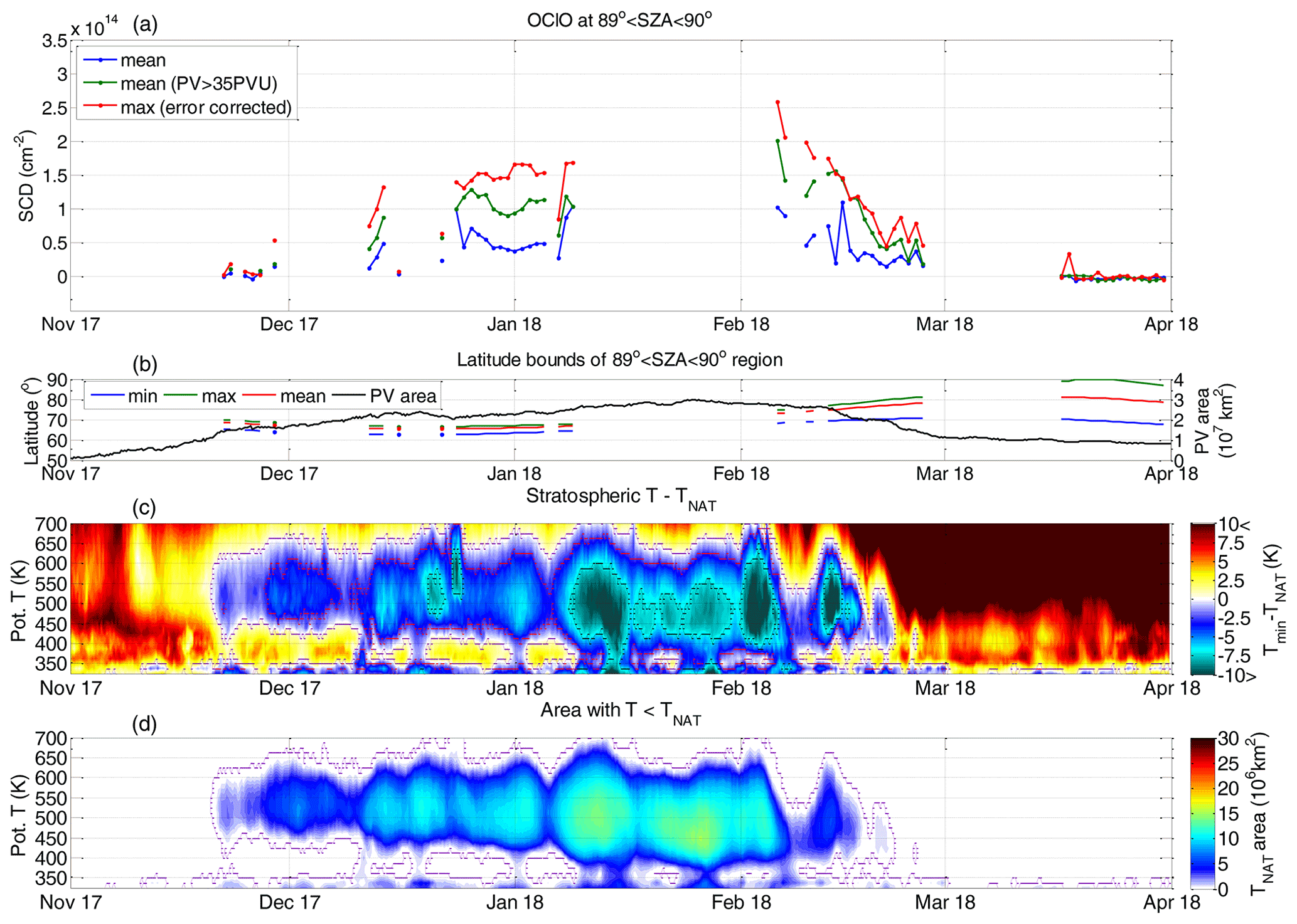
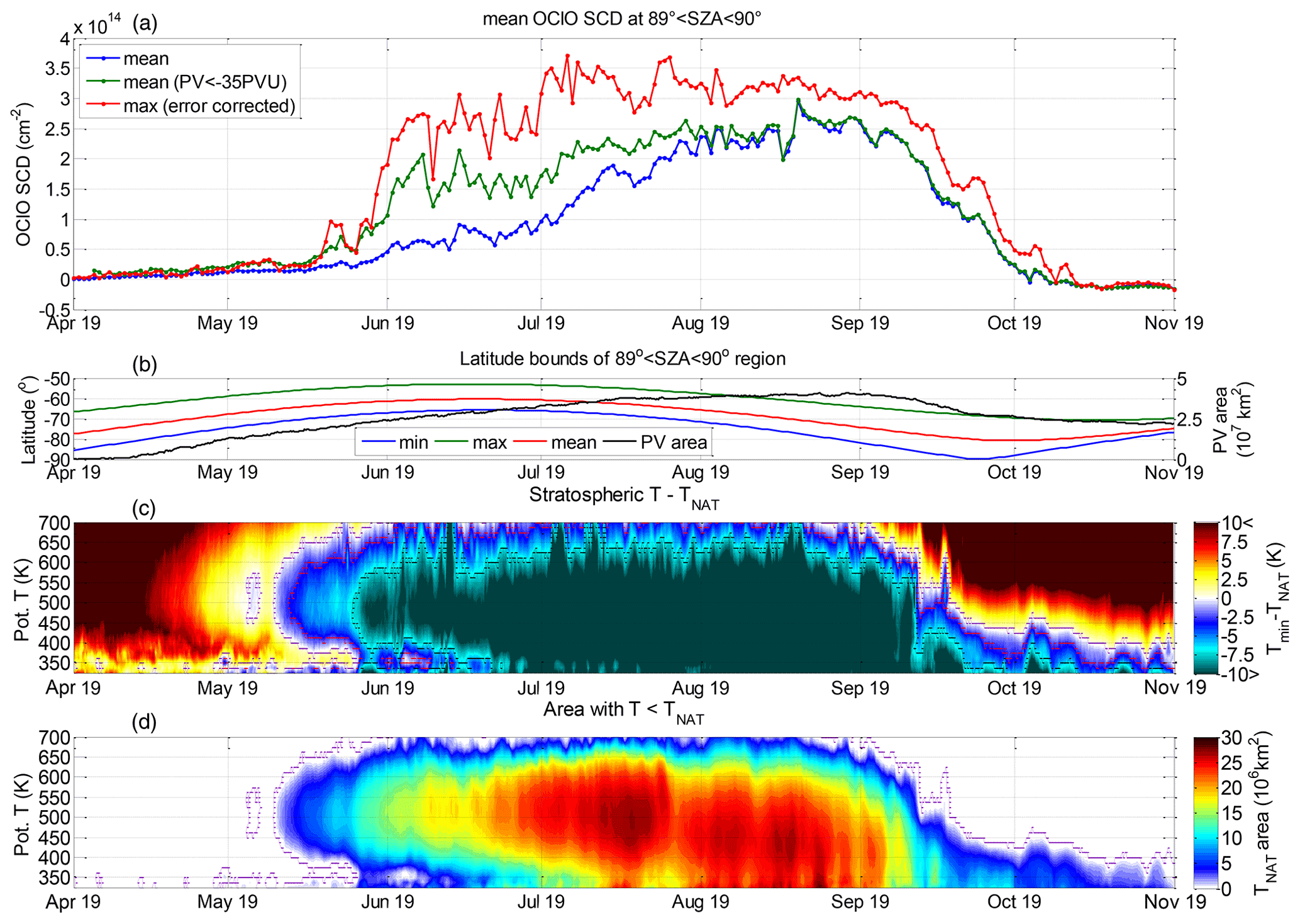
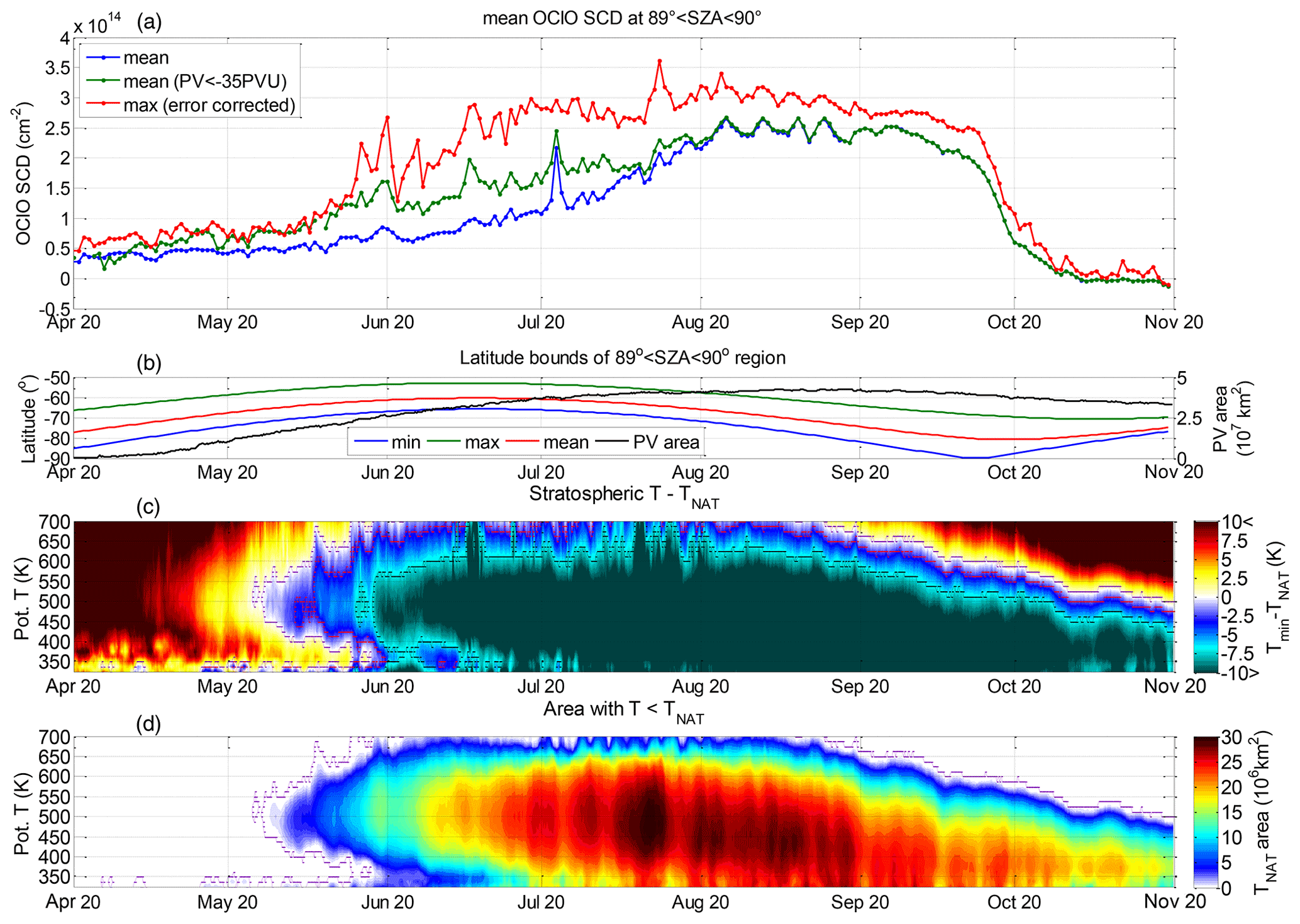
Figure 1 Time series of daily OClO SCDs for the Arctic winter 2017/18 in comparison with the meteorological quantities. Please note that many days of measurements are missing for this winter due to calibration processes after launch. (a) The blue line represents the mean daily OClO SCDs for $\mathrm{89}{}^{\circ }<\text{SZA}<\mathrm{90}{}^{\circ }$, the green line the mean of the measurements within the polar vortex (PV>35 PVU at PT 475 K) and the red line the maximum OClO SCDs (for details, see text). (b) Time series of minimum, maximum and mean latitudes of the TROPOMI pixels which contribute to the mean OClO SCDs shown in (a) (left axis). Also shown is the polar vortex size (area where PV>35 PVU at the PT 475 K) indicated by a black line (right axis). (c) Time series of temperature evolution in the lower stratosphere represented as a difference between the minimum and NAT condensation temperature (T_NAT) as a function of altitude (indicated by the potential temperature). Violet, red and black contour lines indicate T_NAT, $T_{\text{NAT}}^{\prime }$ and the ice freezing temperature T_ICE, respectively. (d) Time series of the size of the area where the temperature is below T_NAT as a function of the potential temperature. Zero is indicated by the violet contour line.

For this winter, unfortunately many days of measurements are missing due to calibration processes. The time series of OClO SCDs daily averages for a SZA between 89 and 90^∘ during this winter are plotted in Fig. 1a. The averages are shown for all data (blue) and data within the polar vortex with PV>35 PVU at a PT level of 475 K (green); the maximum OClO SCD S_max is also plotted (red). In panel (b), the latitudes of the TROPOMI pixels which contributed to the OClO SCDs are illustrated (left axis). In this panel the size of the polar vortex area is also plotted, defined as the area with PV>35 PVU at a PT of 475 K. Panels (c) and (d) provide relevant meteorological information: time series of the (northern) hemispheric minimum temperature expressed as the difference between temperature and T_NAT as a function of the PT. In panel (d), the area where temperature is below T_NAT is plotted, with the violet line showing the boundary of this area.

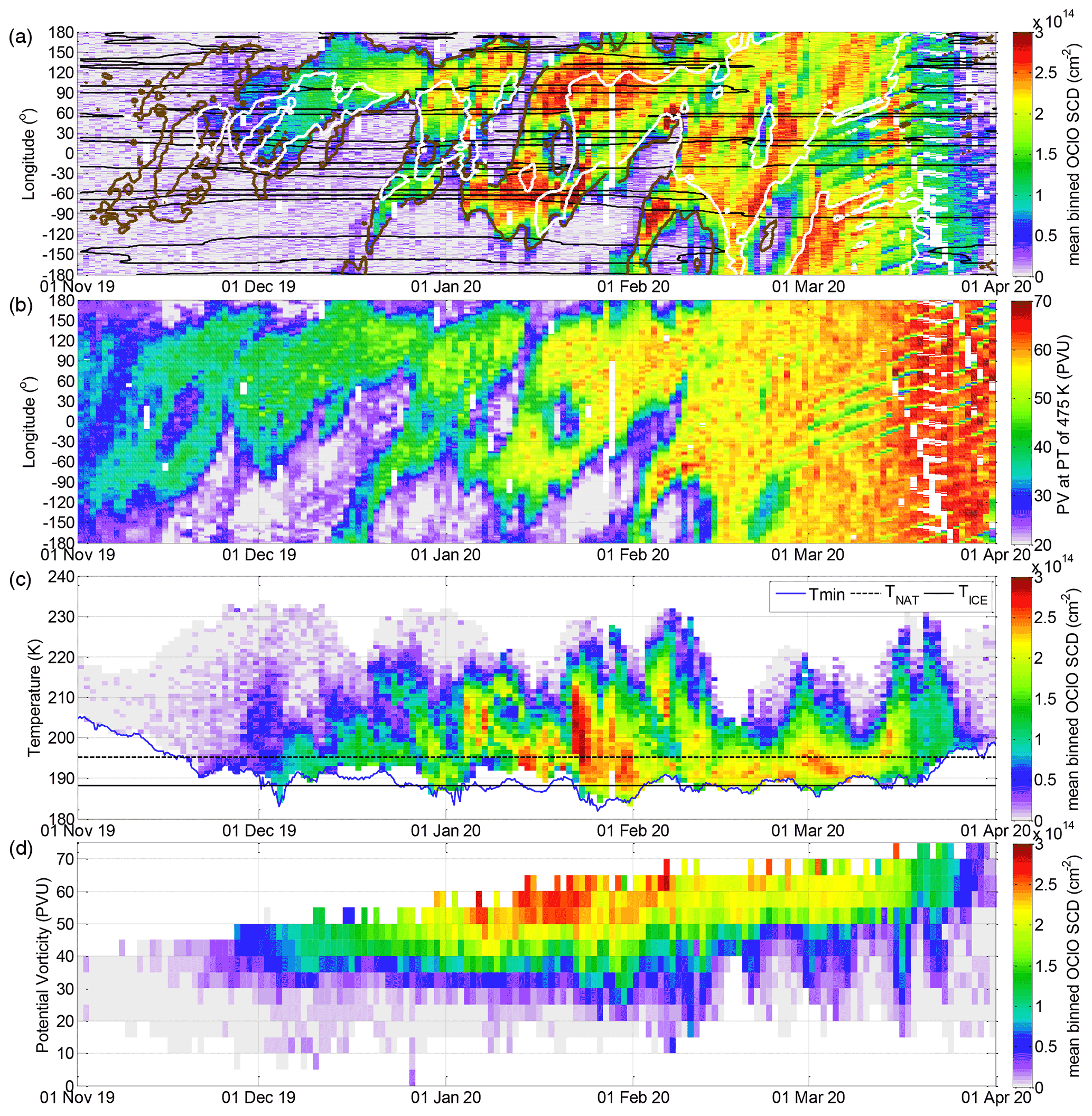
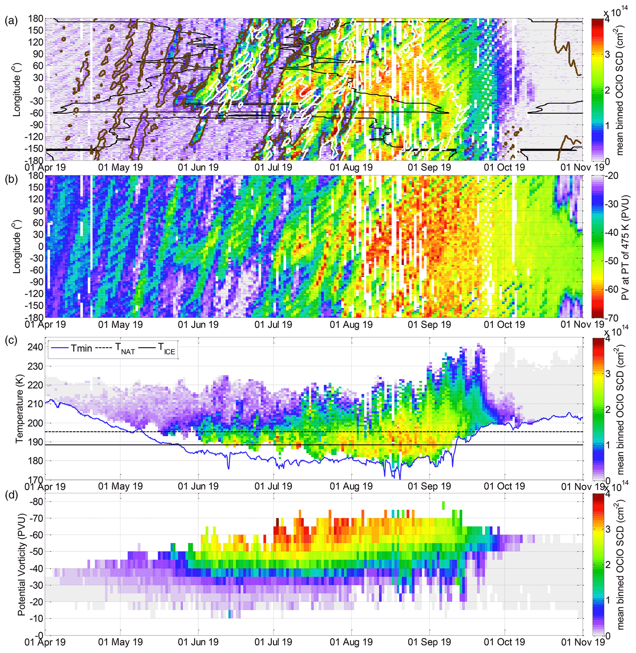
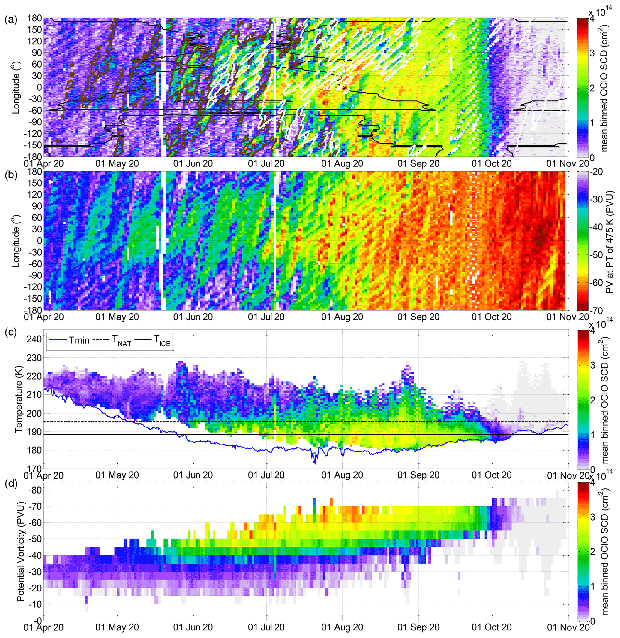
Additionally, in Fig. 2, the temporal variation of the OClO SCDs for $\mathrm{89}{}^{\circ }<\text{SZA}<\mathrm{90}{}^{\circ }$ is presented, resolved with respect to different parameters (longitude, temperature and PV) to allow for a more detailed analysis. Panel (a) resolves the SCDs in longitude (1^∘ grid). The contours are plotted for areas with local temperature below T_NAT (white), for the polar vortex boundaries (PV>35 PVU at a potential temperature level of 475 K, brown) and for a maximum surface elevation of more than 1 km above sea level (black). Panel (b) provides the complete PV information at a potential temperature of 475 K at the place of the measurements of panel (a). Panels (c) and (d) resolve the data with respect to temperature at the measurement location (on 1 K grid at a PT level of 475 K), as well as with respect to the PV (on 5 PVU grid) at the same level. In panel (c), lines indicating T_NAT, T_ICE and minimum temperature (at 19.5 km altitude) are added.

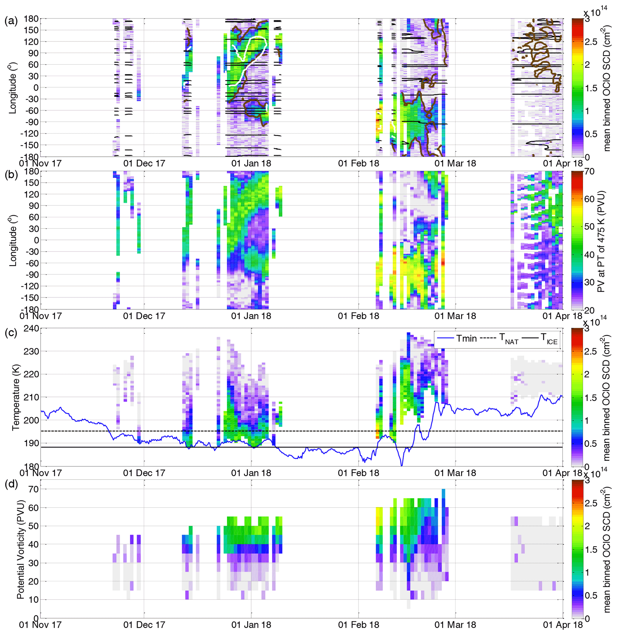
Figure 2 (a) Time series of the daily measured OClO SCDs for $\mathrm{89}{}^{\circ }<\text{SZA}<\mathrm{90}{}^{\circ }$ resolved longitudinally (resolution 1^∘, positive values – east longitudes, negative values – west longitudes) for the Arctic winter 2017/18. Black, brown and white contour lines indicate the maximum surface elevation of 1 km, PV 35 PVU at PT 475 K and temperature T_NAT, respectively. (b) Time series of the potential vorticity at the location of the OClO measurements shown in (a). (c) The same OClO dataset as in (a) but resolved as a function of temperature (resolution 1 K) at a PT level of 475 K. Here the minimum polar hemispheric temperature (minimum temperature for latitudes above 60^∘) at this potential temperature level (blue line) and the values of T_NAT and T_ICE (at 19.5 km) are also indicated. (d) Same OClO dataset as in (a) but resolved as a function of the potential vorticity (resolution 5 PVU).

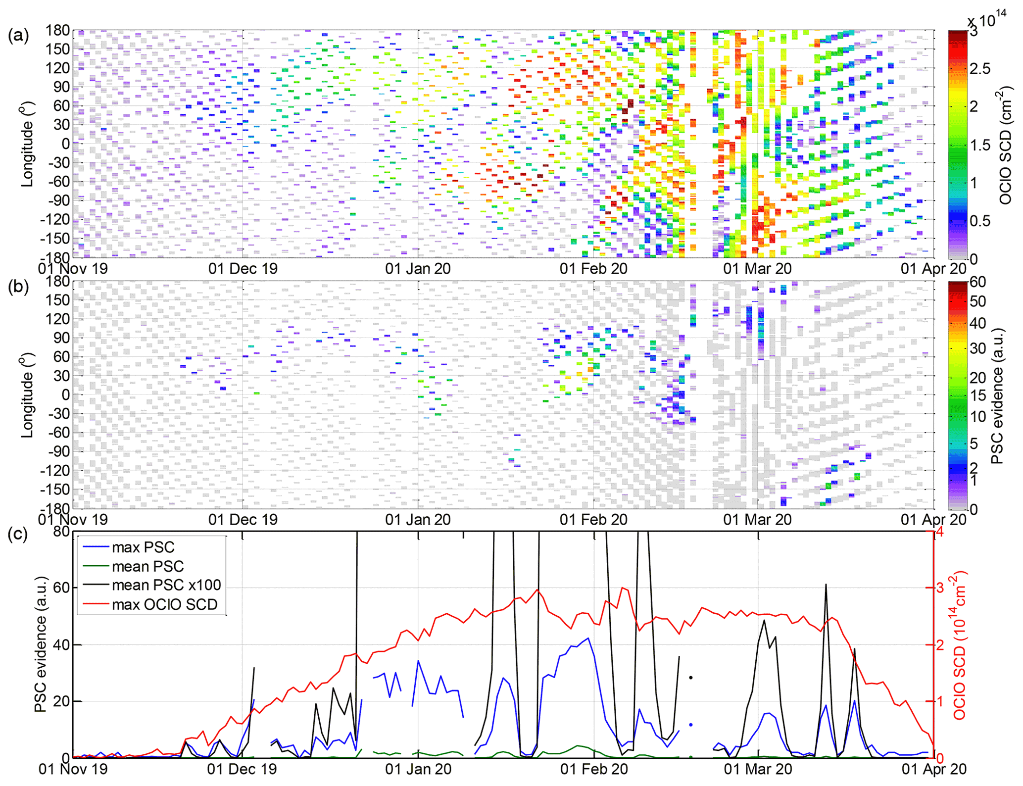
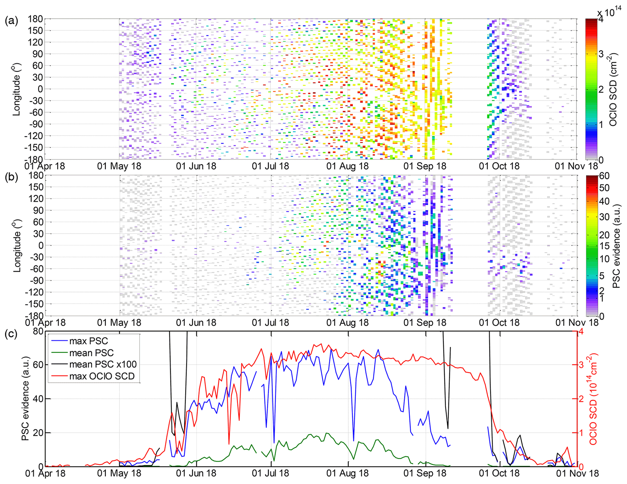
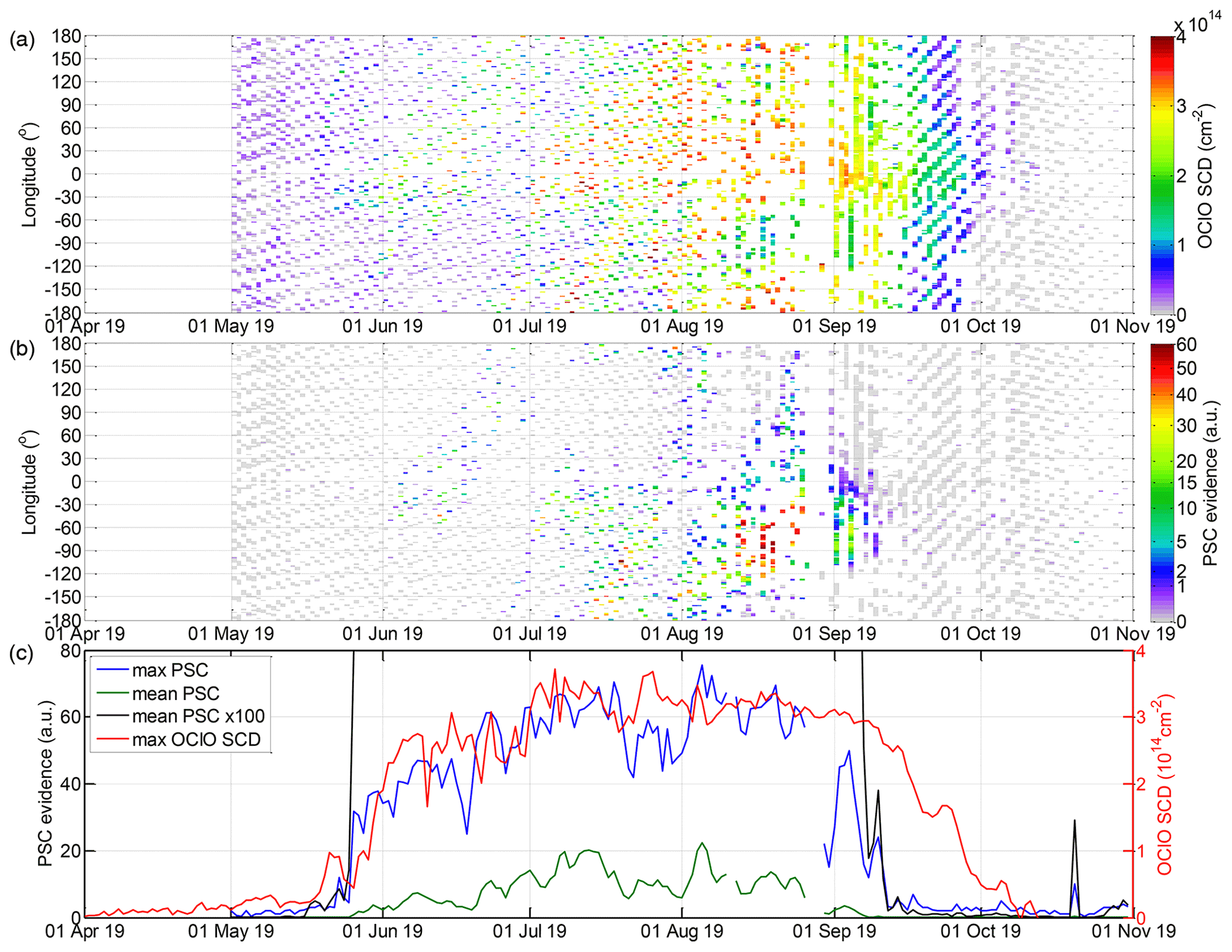
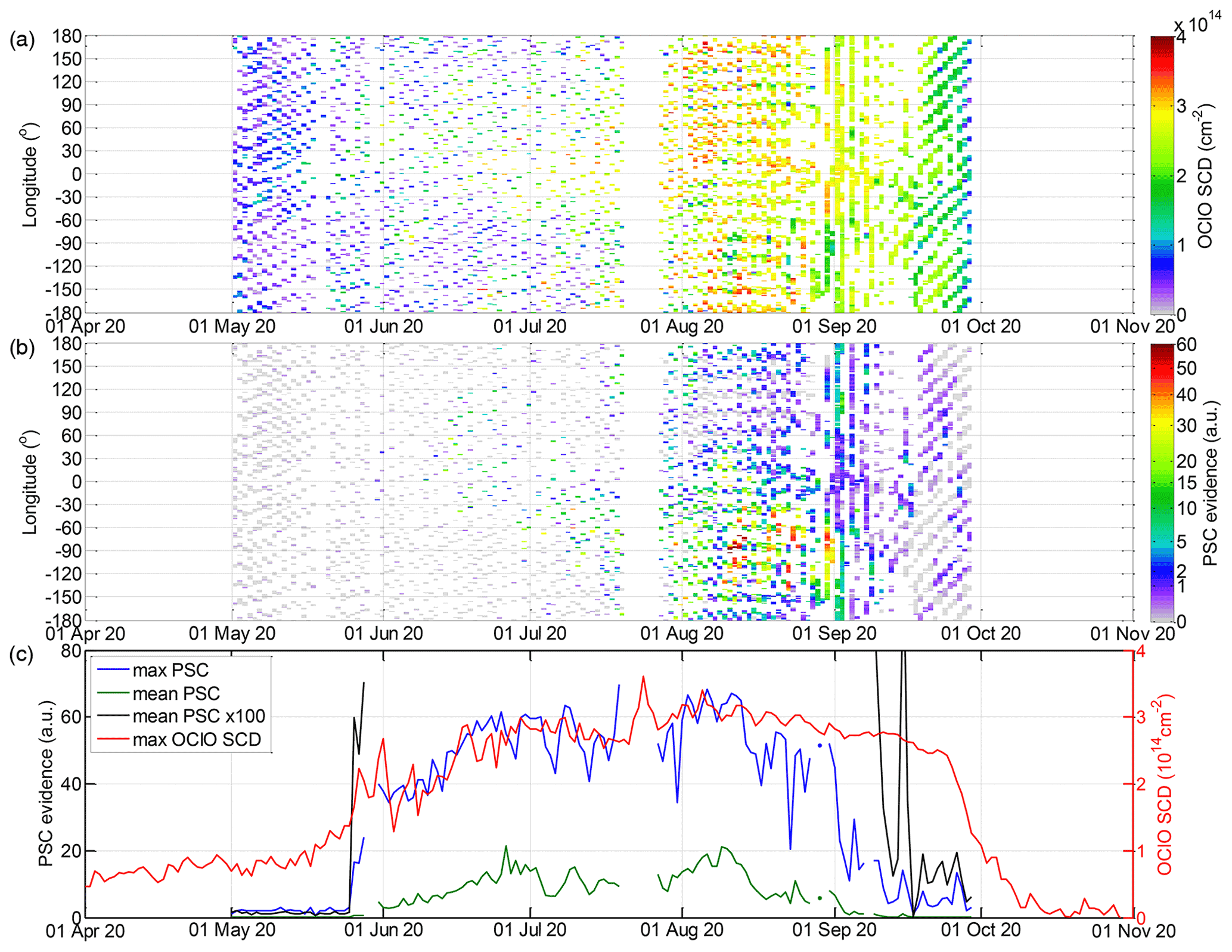
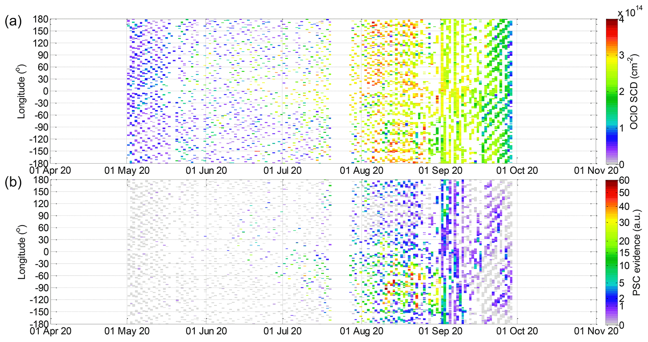
Time series of the PSC evidence resolved in longitude (on a 1^∘ grid) are shown in Fig. 3b. The plots for the respective collocated OClO SCDs are shown in panel (a). The gridded data are shown only for grid points where at least 100 TROPOMI measurements have contributed in order to ensure low random error contribution. Mean and maximum PSC evidence calculated for all CALIOP measurements at latitudes for polar areas of the respective hemispheres above 60^∘ is plotted in the bottom panel (x axis), along with the daily maximum OClO SCDs (y axis).

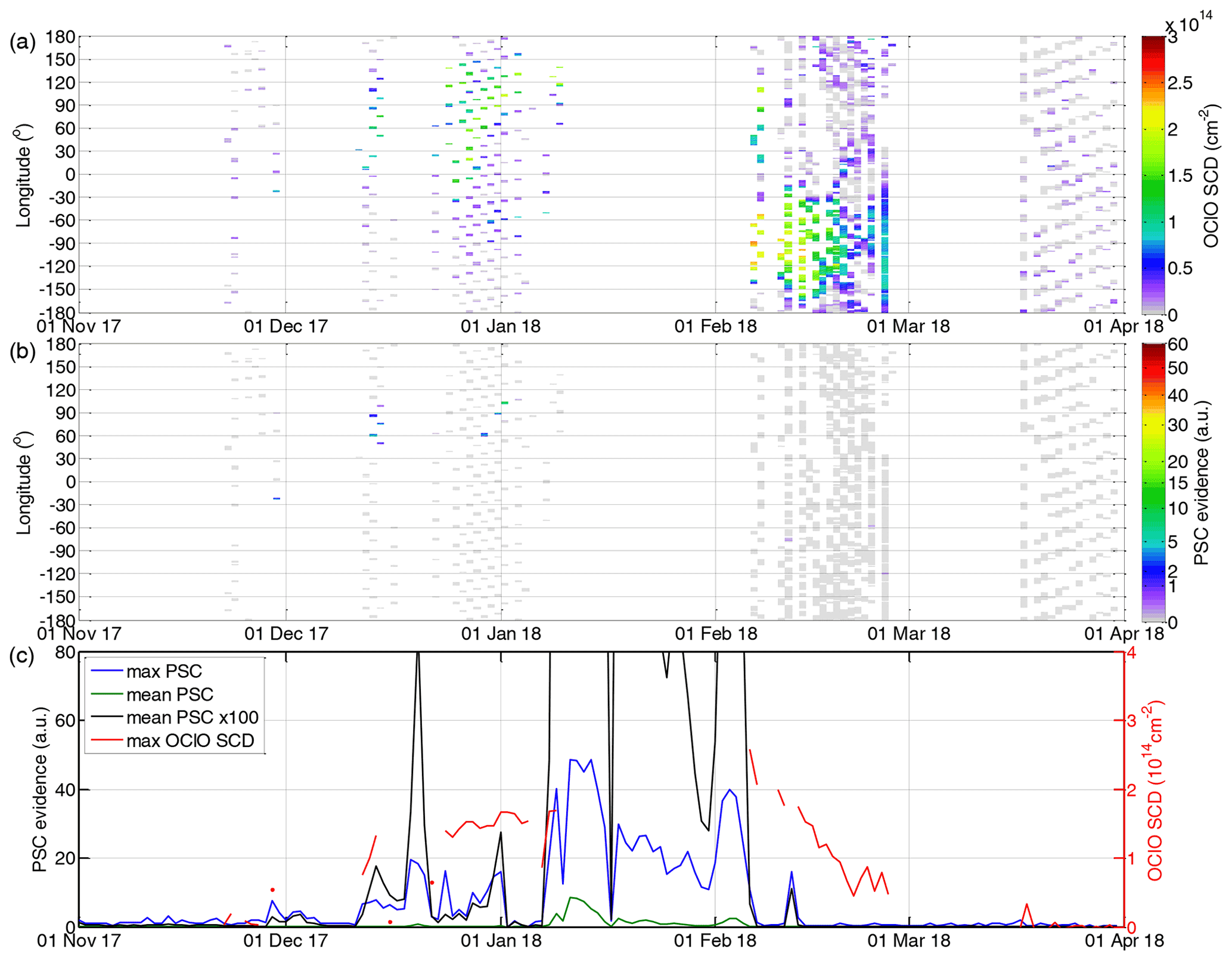
Figure 3 (a) Time series of OClO SCDs for $\mathrm{89}{}^{\circ }<\text{SZA}<\mathrm{90}{}^{\circ }$ being collocated to CALIOP measurements and longitudinally resolved (resolution 1^∘, positive values – east longitudes, negative values – west longitudes) for the Arctic winter 2017/18. (b) Time series of the CALIOP PSC evidence collocated to the OClO SCDs in (a). (c) Left axis: time series of maximum and mean PSC evidence for latitudes above 60^∘ (blue and green lines, respectively), mean PSC evidence derived from the CALIOP PSC mask product scaled by 100 (black line); right axis: maximum OClO SCDs (red line).

The date of 23 November 2017 is the first day we were able to retrieve OClO SCDs with almost complete longitudinal coverage. Although the minimum hemispheric temperature is slightly below T_NAT, we do not see an increase in the OClO SCDs. However, a clear increase is observed on 29 November 2017 above the same area. In this case, a temperature below $T_{\text{NAT}}^{\prime }$ is observed locally at the measurement area, as can be deduced from Fig. 2c, showing increased OClO SCD values at local temperatures around and below $T_{\text{NAT}}^{\prime }$. Thus a chlorine activation process at the locations of the measurements at $\mathrm{89}{}^{\circ }<\text{SZA}<\mathrm{90}{}^{\circ }$ can be expected. There is still a possibility that air masses that have already been activated somewhere else have been transported into the analysed measurement region; however the CALIOP data (Fig. 3) also show evidence of PSC formation at longitudes around 20^∘ W which perfectly matches with the location of the increased OClO SCDs on that day, providing strong evidence of the chlorine activation at this location. For the next available days (12–14 December 2017), even more enhanced OClO SCDs are measured. They are observed almost only within that part of the polar vortex where the temperatures are below T_NAT. The region extends for longitudes between 0 and 120^∘ E. The region where PSCs are evident is slightly smaller (40 and 110^∘ E), suggesting that the enhanced OClO SCDs observed outside this region are either caused by chlorine activation on previous days or due to mixing. For the more eastern regions, still within the vortex, no OClO can be seen, indicating that the observed OClO is still rather fresh and is not yet well mixed with the air masses of the whole vortex. This is not the case anymore around the next available period after Christmas 2017, where enhanced OClO SCDs are observed within the whole vortex and also at temperatures well above T_NAT, which corresponds to a period of a slight vortex warming. PSCs are only evident for few instances in this period, tending to confirm that the bulk of chlorine activation happened earlier. A persistent polar vortex exists until the first week of February, with OClO well distributed within the polar vortex, as visible for the days when measurements are available. The minimum temperature is also below T_NAT for almost all of this time. The seasonal maximum SCD in the presented data is observed at the beginning of February 2018. However, PSC evidence is zero for the collocated CALIPSO measurements. Mean and maximum PSC evidence within the polar region is largely reduced, which is plausible (because temperature has risen above T_ICE, dissolving ice aerosol) with respect to the previous days for which no OClO measurements were available. Nevertheless the local temperature is around $T_{\text{NAT}}^{\prime }$ (i.e. well below T_NAT); thus we do not have an explanation of the complete lack of NAT and STS PSCs for this time period. A sudden stratospheric warming took place on 12 February with a vortex split (Butler et al., 2020; Hall et al., 2021). At the end of the second week, the minimum temperature drops again below T_ICE, before which the vortex area seems to have stayed rather constant for a few days (Fig. 1b). Nevertheless, the OClO values continue to decrease afterwards; the temperature gradient becomes quite large within the split vortex, which can be deduced by the increased OClO at high temperatures in the temperature-resolved time series of OClO SCDs (Fig. 2c). After this short cooling, the temperature rises rapidly, the vortex area decreases and the OClO SCDs continue to decay. The break-up of the polar vortex is also evident in Fig. 2d, where increased OClO SCDs are still found towards lower PV values. A second similar event, but not as strong, is observed in the last days of February (26 February). Here, PSCs are also barely evident at the longitudes (around 120^∘ W) at which the largest OClO SCDs are observed. The vortex eventually strengthens again at the beginning of March when mean zonal winds become westerly again (Butler et al., 2020), but it has no relevance for chlorine activation because of the high temperatures.

4.1.2 Winter 2018/19

The following winter 2018/19 has been reported as being unusual in terms of the polar vortex variability (Lee and Butler, 2020), with both a major sudden stratospheric warming and a reformation of a strong vortex later. In terms of minimum temperature (see Figs. 4c and 5c; for technical explanation of plots, please see the description for the previous winter), the beginning of the winter was rather warm; the temperatures dropped below T_NAT only in December. However the mean OClO SCDs (Fig. 4a) appear to already be slightly but consistently increased above zero during the last days of November, with enhanced OClO SCDs above Greenland and northern Asia (Fig. 5a). This increase however technically is still below the detection limit of 2×10¹⁴ cm⁻². An OClO production in the area covered by the plotted SZA range ($\mathrm{89}{}^{\circ }<\text{SZA}<\mathrm{90}{}^{\circ }$) can likely be excluded because no OClO enhancements at the lowermost temperature bins in the temperature-resolved time series of OClO SCDs are found (Fig. 5c). This finding does not exclude that such an activation could have taken place in some other area not covered by the SZA range investigated here. Lee and Butler (2020) report a begin of the increase of a vertically propagating wave activity during November, and thus local drops of the temperature below T_NAT induced by mountain waves could have been a possibility for OClO formation because the minimum temperature at 600 K reaches T_NAT in that period. The CALIOP data (Fig. 6) however do not show any evidence of PSC formation.

Figure 4 Same as Fig. 1 but for the Arctic winter 2018/19.

Figure 5 Same as Fig. 2 but for the Arctic winter 2018/19.

Figure 6 Same as Fig. 3 but for the Arctic winter 2018/19.

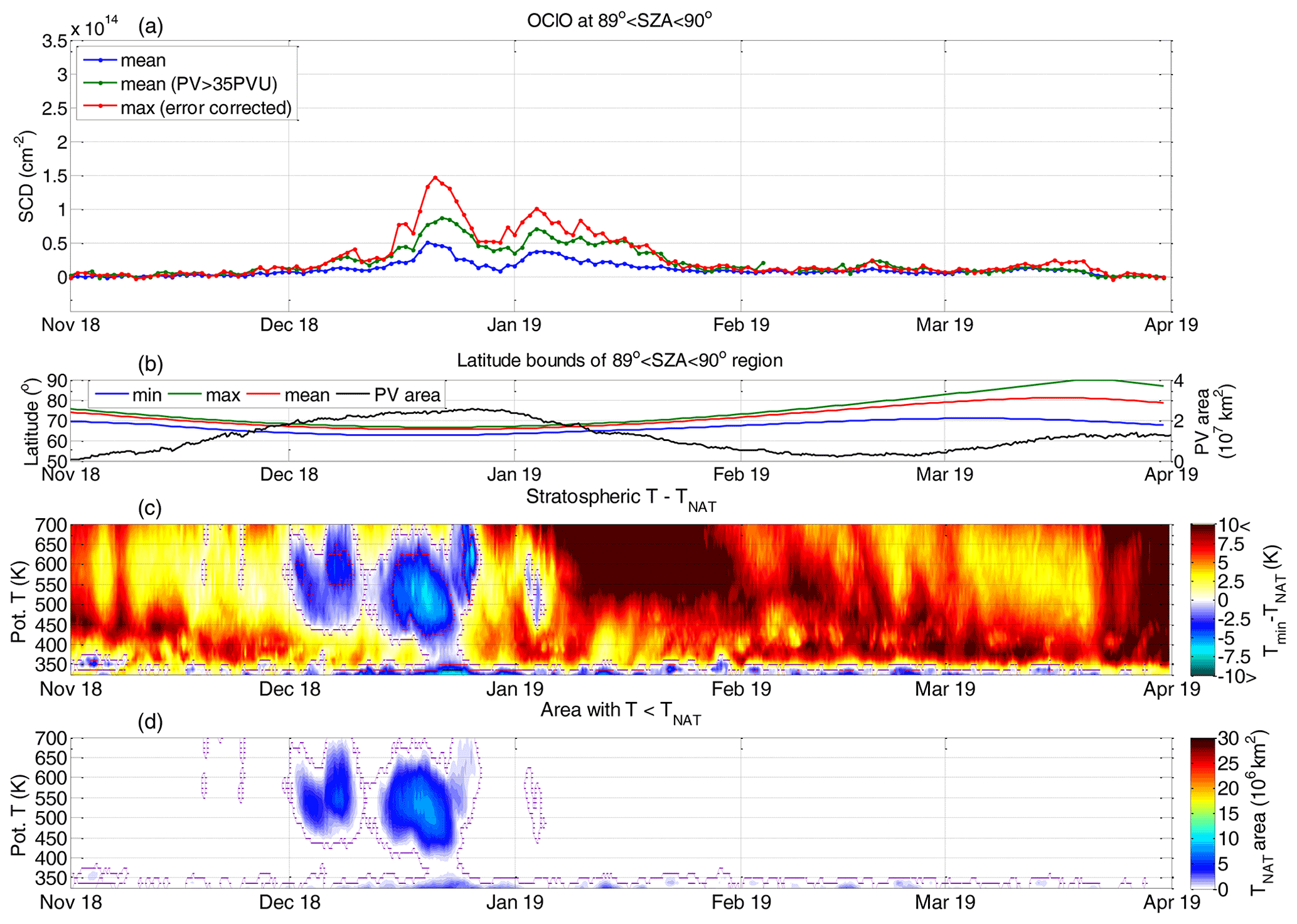
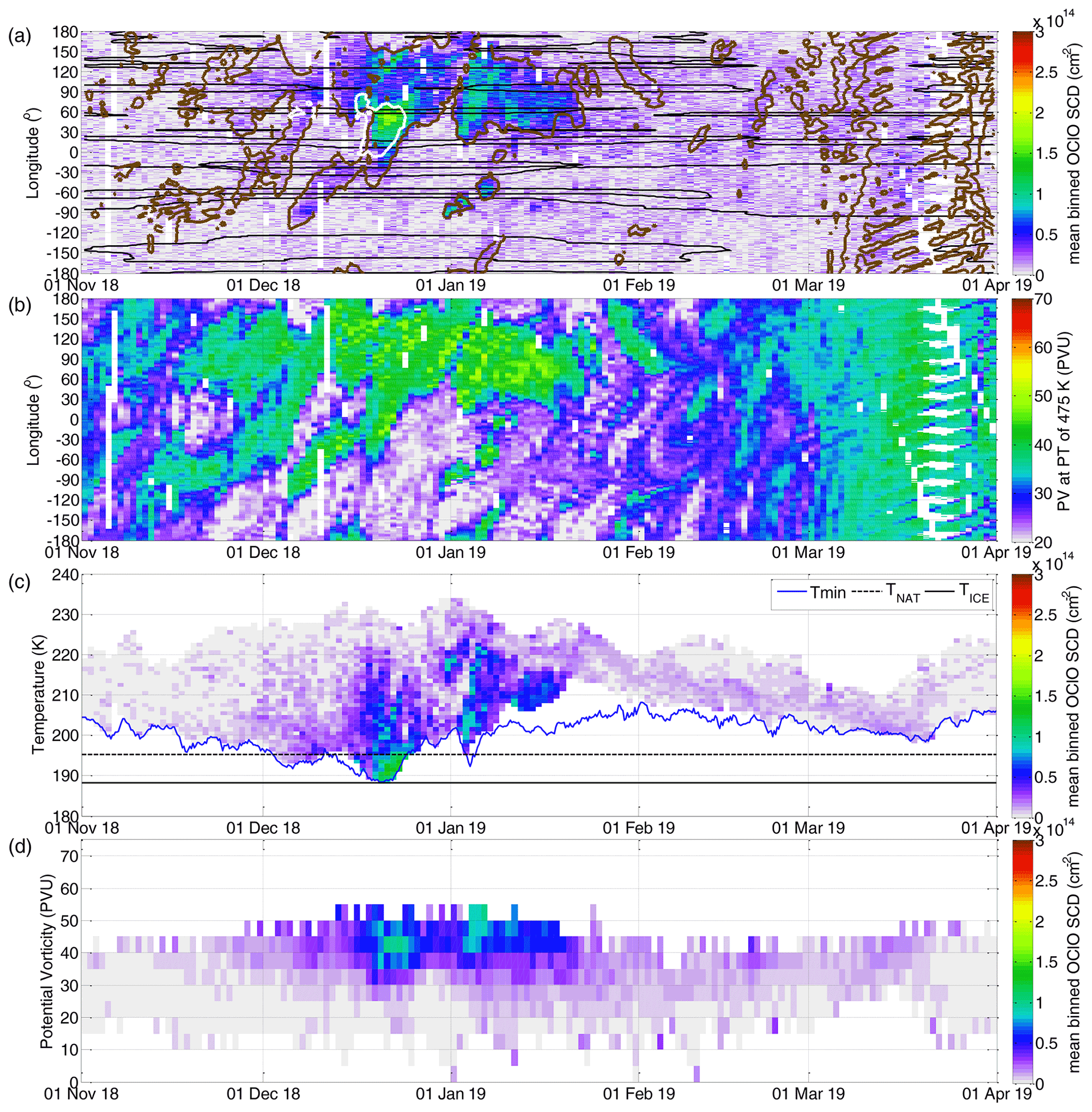
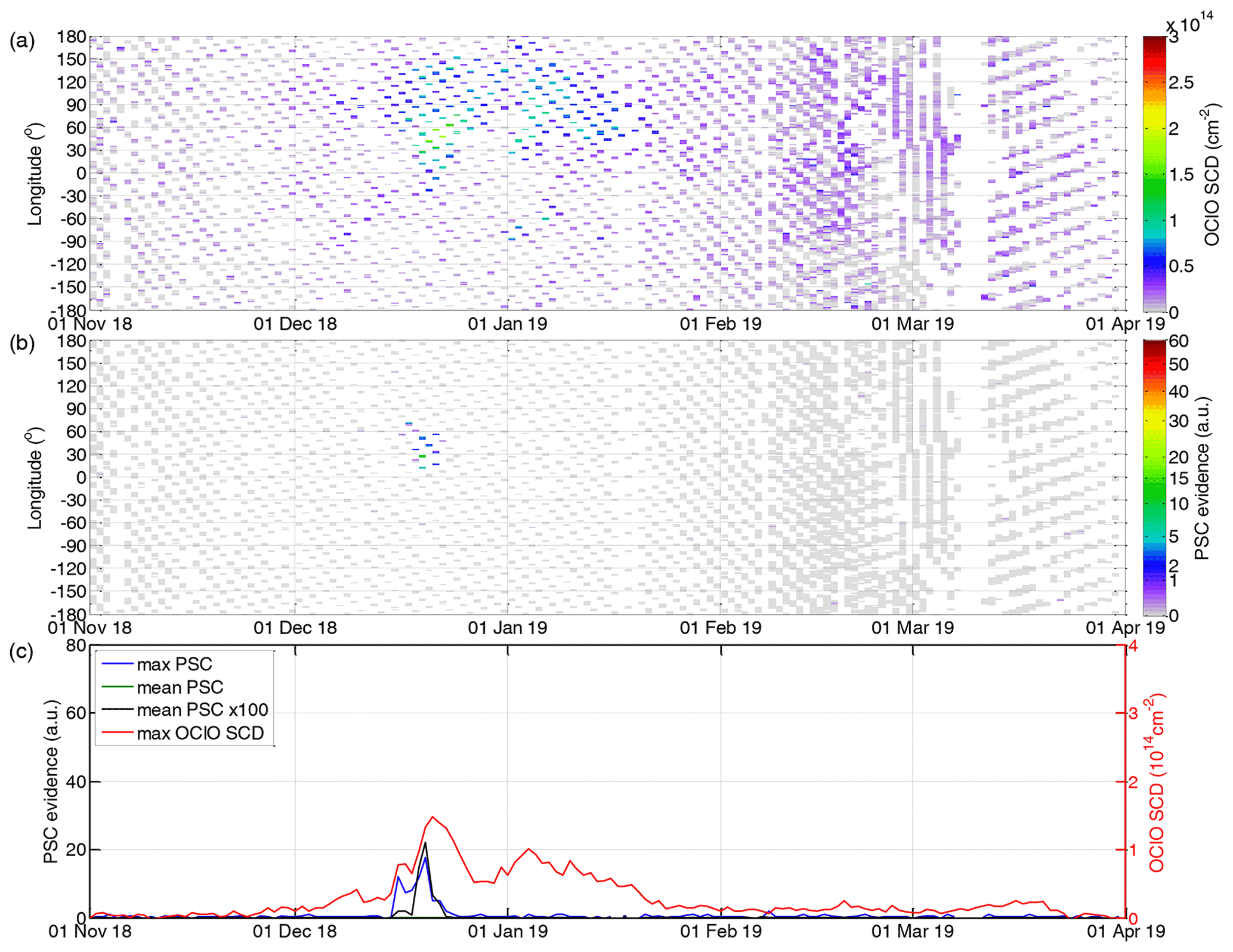
The mean OClO SCDs increase further at the beginning of December a few days after the temperature dropped below T_NAT. This delay probably indicates that the area where this drop occurs is small or that the drop was not sufficient to overcome the supersaturation limit for the PSC build-up. The OClO SCDs are increased for both the areas within the polar vortex as well as for areas of lower temperature (Fig. 5). The OClO SCDs show a clearer increase on 6 December 2018, which coincides with T_min dropping below $T_{\text{NAT}}^{\prime }$. After a small warming, the stratospheric temperatures drop once more (on 15 December) below $T_{\text{NAT}}^{\prime }$, which coincides with a new strong increase in the OClO SCDs on the following day. On 16 December, the mean and maximum evidence of PSCs (Fig. 6c) also has a clear increase above zero. For some of the coldest days (17–24 December) the area of minimum temperatures is covered by the TROPOMI measurements in the range $\mathrm{89}{}^{\circ }<\text{SZA}<\mathrm{90}{}^{\circ }$. The maximum OClO SCDs of this season are observed on 21 December. Local PSC evidence (Fig. 6b) above zero is also observed but only at a few longitudes (10–70^∘ E) for 17–21 December, with a maximum on 19 December. The PSC evidence clearly corresponds to increased OClO SCDs of around 1×10¹⁴ cm⁻² or higher (compare Fig. 6a and b, as well as daily mean and maximum PSC evidence values with the timeline of the maximum OClO SCDs in Fig. 6c). On the other hand, such OClO SCDs or those even higher do not necessarily correspond to an observation of the PSC evidence above zero. The largest OClO SCDs on these days are clearly limited to the area with temperatures below T_NAT, which are located eastwards of the Scandinavian mountains and around the Ural mountains: this could be an indication for mountain waves having enhanced the chlorine activation process. The OClO SCDs in the rest of the analysed polar vortex area remain lower but well above the random uncertainty level and at or above the detection limit. Further, these look like remnants of earlier chlorine activation. After this cooling, the polar vortex slowly starts to shrink (Fig. 4b) and is warmed up at the end of December (Fig. 4c) as the prelude for an early sudden stratospheric warming event reported on 2 January (Lee and Butler, 2020). The atmospheric temperatures rise above T_NAT on 27 December and stay slightly above T_NAT, eventually dropping once more below it on 3 and 4 January 2019. However, the area with temperatures below T_NAT is very small for these days. The appearance of one additional OClO peak at the beginning of January can be attributed to the irregular shape of the polar vortex and to the fact that the earlier activated air masses are moved inside the $\mathrm{89}{}^{\circ }<\text{SZA}<\mathrm{90}{}^{\circ }$ range. This interpretation is supported by the temperature-resolved time series of OClO SCDs (Fig. 5c) where the enhanced OClO SCDs appear at quite warm temperatures. These enhanced OClO values, especially at the end of December and in January, even appear for high temperatures (>20 K above T_NAT). On these days, an increase of the potential vorticity (above 50 PVU) is also observed (Fig. 5d), which indicates that air masses are seen here which were not observed before because they were located deep in the centre of the polar vortex. Afterwards, the OClO SCDs decay until the middle of January to values below the detection limit. In February and March, the formation of a very strong polar vortex has been reported (Lee and Butler, 2020), but the temperatures never fell again below the threshold for the chlorine activation.

4.1.3 Winter 2019/20

In winter 2019/20, an exceptionally strong and cold stratospheric polar vortex was formed which maintained cold temperatures for PSC formation and ozone destruction until the end of March (e.g. Lawrence et al., 2020; Weber et al., 2021). Figures 7 and 8 show the evolution of the OClO SCDs along the cold stratospheric temperatures during the stable polar vortex in winter 2019/20. Figure 9 illustrates the PSC evidence from CALIOP observations. The hemispheric T_min dropped below T_NAT as early as on 16 November 2019, but increased OClO SCDs were observed on 21 November when T_min was already lower than $T_{\text{NAT}}^{\prime }$ (Fig. 7). In Fig. 8c, it can be further seen that this increase happened exactly when the local temperature fell below $T_{\text{NAT}}^{\prime }$. Non-zero PSC evidence (at longitudes 30–60^∘ E and a few days later 0–60^∘ E) also coincides with some of the increased OClO SCDs (Fig. 9). In Fig. 8c, it can further be seen that the OClO SCDs show a new enhancement when the temperatures drop below $T_{\text{NAT}}^{\prime }$ at the beginning of December again. PSCs are also reported (Fig. 9b), as evident at a few longitudes (mainly 60–90^∘ E). With temperatures staying at these low levels or even dropping below T_ICE, the OClO SCDs almost linearly increase until the end of the second week of January 2020. More variation can be seen in the polar mean and maximum hemispheric PSC evidence which increases by an order of magnitude whenever T_min drops below T_ICE. This increase in the PSC evidence however seems not to have a clear relation with the observed OClO SCDs. From mid-January, with temperatures still being low, the OClO SCDs remain nearly constant at about 2.5×10¹⁴ cm⁻² till mid-March. During that period, on several occasions (10 and 20 February and 16 March), air masses with slightly enhanced OClO SCDs appear to be mixed with air from outside the polar vortex (with low PV values) (Fig. 8d). The opposite also happens on 21–26 February, when enhanced OClO SCDs only appear at very high PV values. In the last 2 weeks of March, the stratosphere starts to heat up; there is also no evidence of PSCs in the reported CALIOP data anymore. The OClO SCDs decrease, reaching almost zero at the end of the month, although there is still a small area with temperatures below T_NAT at lower altitudes.

Figure 7 Same as Fig. 1 but for the Arctic winter 2019/20.

Figure 8 Same as Fig. 2 but for the Arctic winter 2019/20.

Figure 9 Same as Fig. 3 but for the Arctic winter 2019/20.

4.2 Antarctic winters

4.2.1 Winter 2018

The Antarctic winter 2018 was relatively stable and colder in comparison to most years of the prior decade with a large and persistent ozone hole (Klekociuk et al., 2021). This accordingly resulted in an expected development of the OClO SCDs, as shown in Figs. 10 and 11. For most of the season, due to the well centred shape of the polar vortex, regions with local temperatures above the hemispheric minimum temperature are observed. Only at the end of August and in September is the area with $\mathrm{89}{}^{\circ }<\text{SZA}<\mathrm{90}{}^{\circ }$ located at regions close to T_min because then the more central parts of the vortex at higher latitudes become illuminated.

The polar vortex starts to form in mid-April (see the development of PV area in Fig. 10b), and temperatures drop below T_NAT in the first 10 d of May (7 May) as shown in Fig. 10c. Shortly afterwards, the temperatures decrease below $T_{\text{NAT}}^{\prime }$, and an increase in the maximum of OClO SCDs within the polar vortex is observed. This signal can also be well identified at the largest PV values. This OClO could have been transported from regions further inside the vortex where it is colder than in the investigated SZA region as the local temperature bins do not yet cover the temperatures below T_NAT. An indication for a local OClO activation would however be the PSC evidence values that were slightly above zero since the beginning of May (Fig. 12b). These values (at longitudes around 15^∘ E–60^∘ W) seem however not to have a clear relation with the collocated OClO SCDs (Fig. 12a) which are larger at other longitudes (60–120^∘ E) than at the collocated longitudes. However, when the local temperatures also drop below T_NAT (starting with 20 May), clearly enhanced OClO SCDs appear, despite the local PSC evidence being above zero only once in these days at the end of May and at a single longitude (10^∘ E), where at the same time the polar mean and maximum PSC evidence increases distinctively. Here the time series of OClO SCDs resolved with respect to temperature also shows larger OClO SCDs at temperatures close to T_NAT. Even “trails” with increased OClO SCDs starting at locations with elevated surface heights (black contour lines in the longitudinally resolved time series of OClO SCDs plot in Fig. 11) and transported eastwards with time are observed, indicating chlorine activation induced by a possible PSC formation due to mountain wave activity. More consistent PSC evidence in these trails is observed to start in mid-June. Local PSC evidence increases during July and in August for almost all collocated OClO SCD observations.

Figure 10 Same as Fig. 1 but for the Antarctic winter 2018.

Figure 11 Same as Fig. 2 but for the Antarctic winter 2018, with the brown line in (a) indicating $\text{PV}=-\mathrm{35}$ PVU, accordingly.

Figure 12 Same as Fig. 3 but for the Antarctic winter 2018.

Figure 13 Same as Fig. 1 but for the Antarctic winter 2019.

Figure 14 Same as Fig. 11 but for the Antarctic winter 2019.

Figure 15 Same as Fig. 3 but for the Antarctic winter 2019.

Increased OClO SCDs are, as expected, limited to air masses with higher PV (i.e. well inside the polar vortex). The exact PV value above which the OClO SCDs are increased changes during the season: in May, high OClO SCDs appear for PV above 40 PVU (it is only cold enough for chlorine activation in the more central parts of the polar vortex). In July, the limit decreases to 35 PVU (as the stratosphere also cools down for air masses with lower PV values). Later, this boundary increases again, along with a strengthening of the polar vortex, which is attributed to rising temperatures for given PV values. It is worth mentioning that this strengthening of the polar vortex in late winter and spring in the Southern Hemisphere (SH) has been attributed to a coincidental seasonal temperature increase in the subtropics (Zuev and Savelieva, 2019), which keeps zonal temperature gradients large, sustaining the development of the polar vortex. The maximum OClO SCDs increase till the end of June and mostly stay constant during July. At the beginning of September, the maximum OClO SCDs begin to slightly decrease but stay at rather high levels until the last week of September, indicating that ClO levels are high enough to enable an effective catalytic ozone destruction. The mean OClO SCDs increase a bit slower till the end of July, which can be explained by the fact that the relationship between PV and the OClO SCDs varies with time and that different areas of the polar vortex (boundary) are observed. Finally, at the end of September until the beginning of October, a rather quick chlorine deactivation occurs, despite the fact that the temperatures are still below T_NAT and the polar vortex is stable. Besides a relation with the decrease in PSC evidence as observed by CALIOP (or at least PSCs descending to lower altitudes not covered by the considered altitude range of >4 km above the tropopause) at the end of September, the mechanism of chlorine deactivation as described by Grooß et al. (2011) can also play a role: when an almost complete destruction of ozone occurs, almost all chlorine becomes bound in HCl and cannot be reactivated.

4.2.2 Winter 2019

Winter 2019, however, was quite unique as a minor sudden stratospheric warming was observed, which was just a bit weaker than the major sudden stratospheric warming in 2002 (Lee, 2020; Klekociuk et al., 2021). A very small ozone hole area in September in comparison to that of 2018 has also been reported, but the magnitude of the vortex-averaged chemical ozone depletion was not significantly different between the years. Wargan et al. (2020) attributed most of the smaller ozone loss to dynamics. This is in accordance with Sinnhuber et al. (2003), who reached similar conclusions with respect to the major stratospheric warming in 2002.

The daily mean and maximum OClO SCDs (see Fig. 13) show a similar temporal development as in 2018 until 6 September. Clearly increased OClO SCDs at local temperatures below T_NAT (middle May) and even more increased OClO SCDs at local temperatures below $T_{\text{NAT}}^{\prime }$ (from the beginning of June) are also observed (Fig. 14). From the beginning of June, evidence for PSCs at the locations with increased OClO SCDs is also consistently observed (Fig. 15). After the stratospheric warming (6 September), the area with temperature below T_NAT decreases rapidly, and the hemispheric minimum temperature rises above T_NAT (at PT 475 K) by the end of the third week of September. The decrease and the rise are accompanied by a strong decrease of the OClO SCDs, with a rather constant rate till the end of September. After 6 September, the PSC evidence (both local and the polar mean and maximum) observed by CALIOP also becomes almost zero. At the beginning of October the OClO SCDs decrease further at a lower rate. Interestingly, two distinct temperature drops at lower altitudes (at PT around 400 K) lead to two small short-term increases in the mean and maximum OClO SCDs.

Figure 16 Same as Fig. 1 but for the Antarctic winter 2020.

Figure 17 Same as Fig. 11 but for the Antarctic winter 2020.

Figure 18 Same as Fig. 3 but for the Antarctic winter 2020.

Looking at the parameter-resolved (longitude, temperature and PT) time series (Fig. 14), one can notice that the high OClO SCDs already appear at rather high local temperatures and low PV values on 11 August and more clearly on several days after 18 August. A mixing towards low PV values after 5 September can also be seen, being especially strong at the beginning of the second week of this month, which coincides with the sudden stratospheric warming episode. The small chlorine activation events at the beginning of October can be well distinguished in all parameter-resolved time series of OClO SCDs, occurring at the lowermost temperatures and the highest PV values. We can speculate that this potential for further chlorine activation indicates that not all ozone in the polar vortex was destroyed by the initially activated chlorine. This indicates that chlorine could in principle be reactivated again if the temperatures become low enough, as is usually the case in the Arctic.

4.2.3 Winter 2020

While so far no scientifically peer-reviewed analysis of this winter could be found, the SH winter 2020, although with a usual development at the beginning, has been reported by meteorological surveys (e.g. Copernicus, 2021) as having one of the largest, deepest and longest persisting ozone holes of the past 40 years during the time period of October to December. The earlier months of this winter however show a vortex development, which corresponds to typical Antarctic conditions. Nevertheless, rather similar timing and levels of OClO SCDs and PSC evidence as for August to October 2018, thus also during the deactivation period (Figs. 16, 17 and 18), are observed. During June to August, lower OClO SCDs are observed at the coldest temperatures and at the highest potential vortex values for this winter than in 2018. An exception however is the already slightly increased OClO SCDs in April (already since the middle of March, not shown here). So far we do not have a clear explanation for this finding, except increased backscatter ratios in CALIOP data in May 2020 compared to those in previous years. For the polar mean PSC evidence (black line in Fig. 18c), values distinguishable from zero can already be observed at the beginning of May, which was not the case for the previous SH winters. The local PSC evidence (Fig. 18b) has sporadic values slightly above zero, which however seems not to be correlated with the collocated SCDs (Fig. 18a). We also do not see a clear local correlation between the backscatter ratios and OClO SCDs when they are at low levels (see Appendix B). The meteorological conditions plotted in Fig. 16 seem to be similar as for the years before, with temperature well above T_NAT. At the beginning of April, the spatial distribution of the increased OClO SCDs is also not associated with areas of high PV within the polar vortex (Fig. 17d). The OClO SCDs decrease to zero again in October as for the years before, largely excluding the possibility of a systematic instrumental effect. Note that a similar increase is also consistently observed in the preliminary Sentinel5P Innovation activity (S5p+I) operational TROPOMI OClO product (Mayer et al., 2020) OClO SCD data, and the ground-based zenith sky observations at Neumayer station in Antarctica show a slightly larger diurnal variability in April and May than for the previous two winters as shown in Puķīte et al. (2021).

5 Conclusions

We related our new dataset of TROPOMI OClO SCDs to meteorological parameters driving polar vortex dynamics and thus also PSC formation and chlorine activation. OClO SCDs are also compared directly to PSC measurements from CALIOP on CALIPSO. The great advantage of satellite observations was exploited in the way that, in addition to the temporal evolution of the chlorine activation, its spatial features were also investigated. The TROPOMI OClO SCDs are generally well correlated with meteorological parameters. The most important findings are that the chlorine activation signal appears as a sharp gradient of the OClO SCDs once the local temperature drops approximately below $T_{\text{NAT}}^{\prime }$ (3 K below T_NAT), thus being in agreement with previous research. For the Northern Hemisphere (NH), the sharp increase is also well related to such a dropping of the hemispheric minimum temperature (possibly because of a better mixing of air masses within the vortex), while in the SH, a weaker relation with respect to the hemispheric minimum temperature is found. A relation with the lee sides of mountains can also be observed at the beginning of the winters, indicating a possible association of OClO formation with lee waves.

The comparison of the OClO SCDs to PSC measurements from CALIOP on CALIPSO reveals that increased OClO SCDs in most instances coincide well with CALIOP measurements where PSCs are detected. Increased OClO SCDs however do not always coincide with enhanced PSC evidence. While in many cases increased OClO SCDs without coinciding PSC could be caused by transport or mixing and the presence of PSCs somewhere else in the polar region, at the beginning of winter, the observed moderate-level OClO SCDs could not be clearly associated with the presence of PSCs detected by CALIOP.

High OClO SCDs reaching 3×10¹⁴ cm⁻² at maximum are observed for the very cold stratospheric NH winter 2019/20 with its very stable polar vortex, thus being close to the maximum values found for the SH winters.

An extraordinary winter was observed in the SH in 2019, with a minor sudden stratospheric warming at the beginning of September. Until this event, similar OClO SCDs in this winter were observed compared to the previous winters, but the deactivation occurred about 1–2 weeks earlier in this winter.

Further investigations are still needed with respect to the exceptional OClO increase, which goes along with increased backscatter ratios compared to previous winters but is not correlated with the stratospheric meteorology in late March and April in 2020 in the SH, where a larger OClO SCD signal above the typical uncertainty range was observed ($\sim \mathrm{5}\times {\mathrm{10}}^{\mathrm{13}}$ cm⁻²), which is also observed in the S5P+I data.

Appendix A: Radiative transfer effects on the sensitivity area of OClO SCDs

At high SZAs, direct sunlight crosses the atmosphere at very slant paths. Afterwards (with or without undergoing additional scattering before), it is scattered along the line of sight towards the instrument. The distribution of the light that is detected by the instrument is expected to vary both vertically and horizontally, depending on the scattering and absorbing properties of the atmosphere and the ground (e.g. the air density, trace gas concentration or PSC presence and ground albedo), of the light (i.e. wavelength) and of the solar and viewing geometries. OClO slant column densities (SCDs) can most directly be interpreted as OClO number densities integrated along the light paths that contribute to the measurement. Thus the contribution of a certain area to the measurement depends both on the light paths that cross this area and the OClO number density there.

We use the 3D full spherical radiative transfer model (RTM) McArtim (Deutschmann et al., 2011; Deutschmann, 2014) to quantify the spatial sensitivity of the measured OClO SCDs by obtaining so-called box AMFs B_i:

$$\begin{array}{}\text{(A1)}& B_i={\displaystyle \frac{L_i}{\mathrm{\Delta }{h}_i}},\end{array}$$

where L_i is the effective light path in the 2D box i with a vertical resolution Δh_i, also being horizontally resolved along the direction from the line-of-sight coordinate towards the Sun.

Box AMFs obtained for an aerosol-free atmosphere (with a 1 km vertical resolution and a 0.2^∘ (22 km) horizontal resolution) at a SZA of 89.5^∘ at the measurement location are illustrated in Fig. A1a. As expected, the largest box AMFs (effective light paths) occur near the line-of-sight position at altitudes of around 19 km. Areas through which the light has travelled also have increased box AMF values.

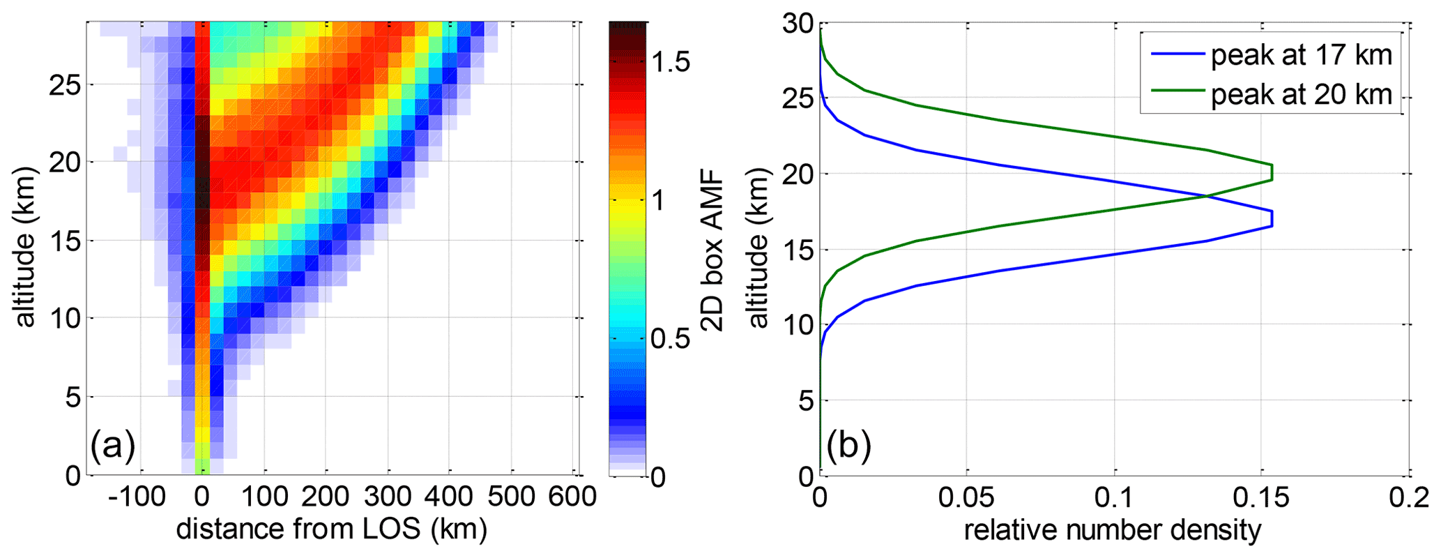
Figure A1 (a) 2D box AMFs for a clear-sky atmosphere. (b) Relative OClO number density profiles used for the sensitivity studies.

To evaluate the contribution of these areas to the OClO SCDs, we need to multiply these box AMFs with the local OClO number densities. To consider the variability in the OClO distributions, we base our calculations on OClO number density profiles which are shifted in altitude. We consider here two Gaussian shape profiles with a full width at half maximum (FWHM) of 6 km and peaks at 17 or 20 km. The profiles are illustrated in Fig. A1b. With regard to the horizontal variability, we assume that the OClO photolysis rate varies linearly from 0.015 to 0.05^∘ s⁻¹ between SZAs of 90 and 85^∘, consistent with the calculations in Kühl et al. (2004a); thus OClO decreases in the direction of the Sun proportionally to the inverse of the photolysis rate. Note that atmospheric dynamics could increase the gradient even further (as typically potential vorticity decreases towards lower latitudes), so the evaluation here would represent the largest horizontal extension scenario.

Figure A2a and c show the obtained partial SCDs (products of box AMFs and local OClO number densities) calculated for the profile with the peak at 17 km (a) and 20 km (b), respectively. Horizontally and vertically integrated SCDs are shown on the right (panels b and d, respectively). A clear maximum at the line-of-sight location is obtained at altitudes slightly above the simulated profile peak, with an exocentric distribution towards the direction of the Sun. We find that the mass centre of the sensitivity area for this simulation is located 100 km (for the profile with peak at 20 km) and 80 km (peak at 17 km) from the line-of-sight coordinate.

Figure A2 (a, c) Simulated partial SCDs (products of the box AMFs and the local OClO number density values) calculated for the profile with the peak at 17 km (a) and 20 km (c). (b, d) Horizontally (b) and vertically (d) integrated partial SCDs with mass centres indicated.

The possible presence of PSCs in the stratosphere is supposed to provide a strong effect on the scattering properties and thus also an effect on the stratospheric OClO measurements. Therefore, we have performed tests with variable PSC amounts based on the aerosol climatology as presented in Vanhellemont et al. (2005) inside the polar vortex. We found that the mass centre for cases with PSCs present is now slightly closer to the line-of-sight location. Assuming PSC profiles with a PSC extinction that is 3 times larger than the presented median values in the climatology, the mass centre of the sensitivity area is located 60–80 km (depending on the assumed peak altitude) from the line-of-sight coordinate. Thus, the effect is rather limited.

To test the effect on the comparison plots, we considered as the measurement location the coordinate that is 100 km towards the Sun from the line-of-sight coordinate, i.e. the maximum possible displacement of the mass centre of the sensitivity distribution. We repeated the calculations with this assumption for winter 2019/20 in the NH and 2020 in the SH. The plots are shown in Figs. A3 and A4. The results for the shifted measurement coordinate follow those with the considered measurement location at the line-of-sight coordinate very well (as in Figs. 8 and 17). Only a shift by about 1 K temperature between the results is observed. The shift in PV is somehow larger near the polar vortex boundaries (due to the larger gradient) but is still below the resolution of the PV used in the plots (5 PVU).

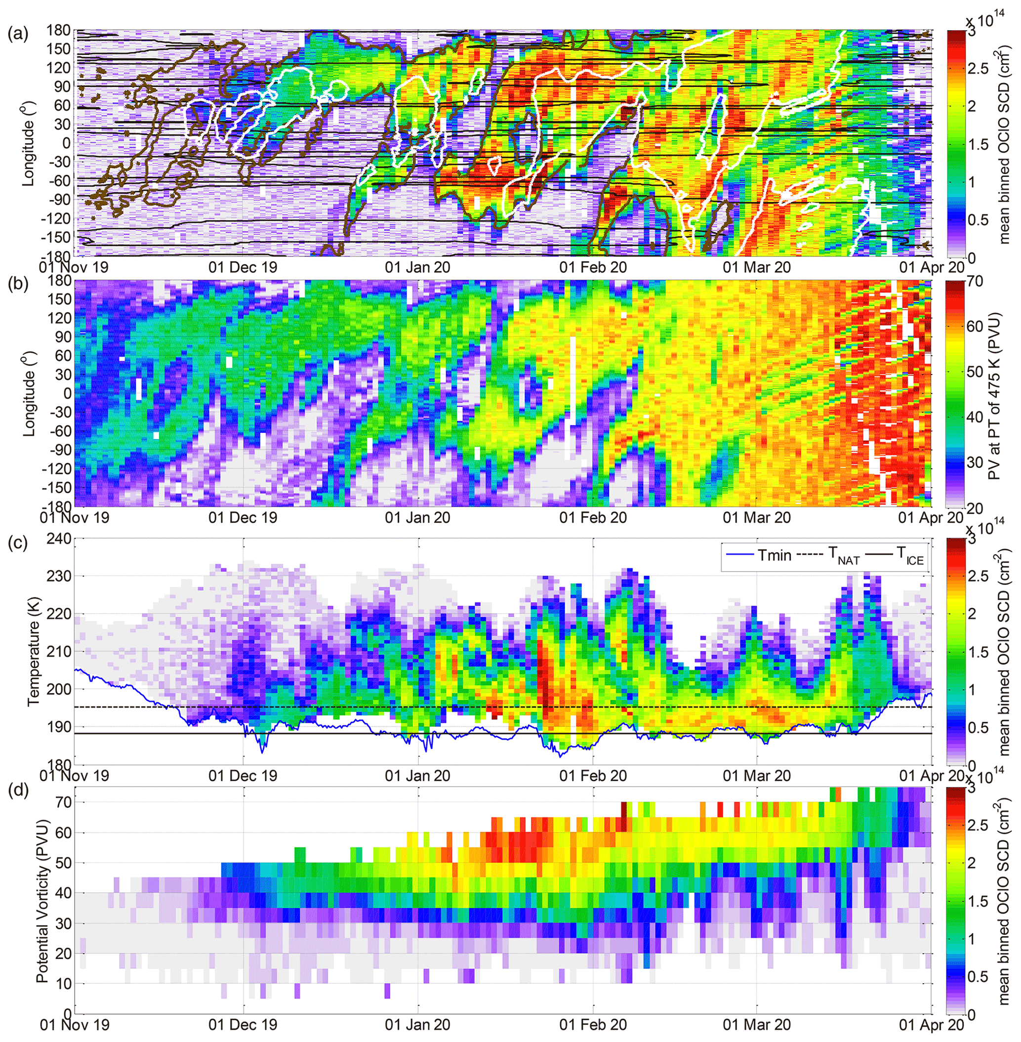
Figure A3 Same as Fig. 8 but with the assumed measurement location coordinate shifted by 100 km from the line-of-sight coordinate towards the Sun.

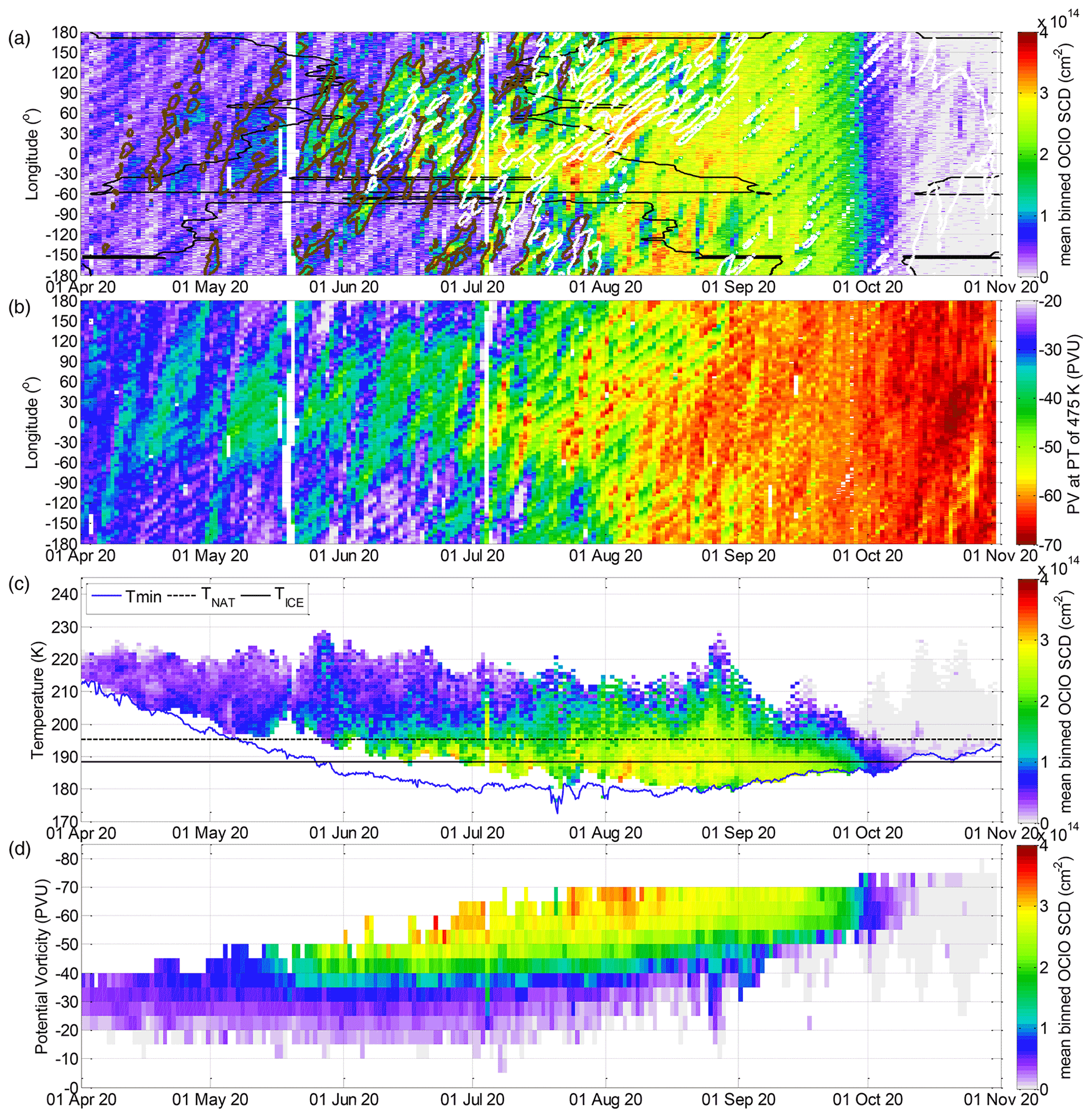
Figure A4 Same as Fig. 17 but with the assumed measurement location coordinate shifted by 100 km from the line-of-sight coordinate towards the Sun.

For the comparison to the PSC evidence, the shift of 100 km towards the Sun also has no substantial effect (compare Fig. A5 for winter 2020 in SH with the corresponding plots in Fig. 18) despite the lower PSC evidence values in the first half of the winter.

Figure A5 Same as Fig. 18a and b but with the assumed measurement location coordinate shifted by 100 km from the line-of-sight coordinate towards the Sun.

Appendix B: PSC evidence and aerosol backscatter ratio in comparison to OClO SCDs

Here, we investigate how well the PSC evidence can represent PSCs in comparison to the aerosol backscatter ratios for the comparison with the OClO SCDs in a case study for months during the PSC activation period (May–July 2020 in SH). Therefore, the mean backscattered ratio for the same altitude range (i.e. for altitudes above 4 km above the tropopause) and for the same collocation criteria as for the PSC evidence (Sect. 3) was calculated from the CALIOP data. The OClO SCDs and the mean backscatter ratios are plotted in Fig. B1. In Fig. B2a and b, the correlation plot between the PSC evidence and the mean backscatter ratios is shown, (a) for May–July 2020 and (b) only for May 2020. Please note the different x and y axis scales. It is found that in the case of low mean PSC backscatter values (in May), no good correlation with the PSC evidence can be seen. Since PSCs are detected by testing whether the total backscatter ratio and/or the perpendicular backscatter are above a certain threshold at individual altitudes (Pitts et al., 2009), it is understandable that for the mean backscatter ratios there is no clear threshold. By also including time periods with large PSC backscatter values, however, a more clear relationship can be seen. Only few cases with very large mean backscatter ratios fall out of the slope because the representation of the PSC abundance by the PSC evidence is limited by the different spatial averaging intervals, with the minimum being the spatial resolution of the individual measurement. Thus, the PSC evidence for very dense PSC clouds is underestimated.

In order to understand which quantity better relates with the OClO SCDs, we plot the correlation between the OClO SCDs and either the PSC evidence (Fig. B2c and d) or the mean backscatter ratio (Fig. B2e and f). In the case of low PSC/stratospheric aerosol levels (especially in the plots for May 2020), there is a better relation between the OClO SCDs and the PSC evidence: in the case of increased PSC evidence, OClO SCDs are generally increased (distinct from zero). For the mean backscatter ratio, the scatter of the data points is too large to see a relation between this quantity and the OClO SCDs for May. Given the somehow better sensitivity of the PSC evidence for low PSC levels, we conclude that the PSC evidence is a well-suited quantity for the detection of PSCs from CALIOP.

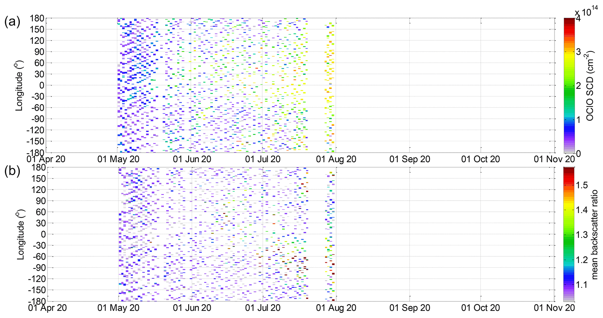
Figure B1 (a) Same as Fig. 18a but with data for May–July 2020. (b) Collocated mean backscatter ratios.

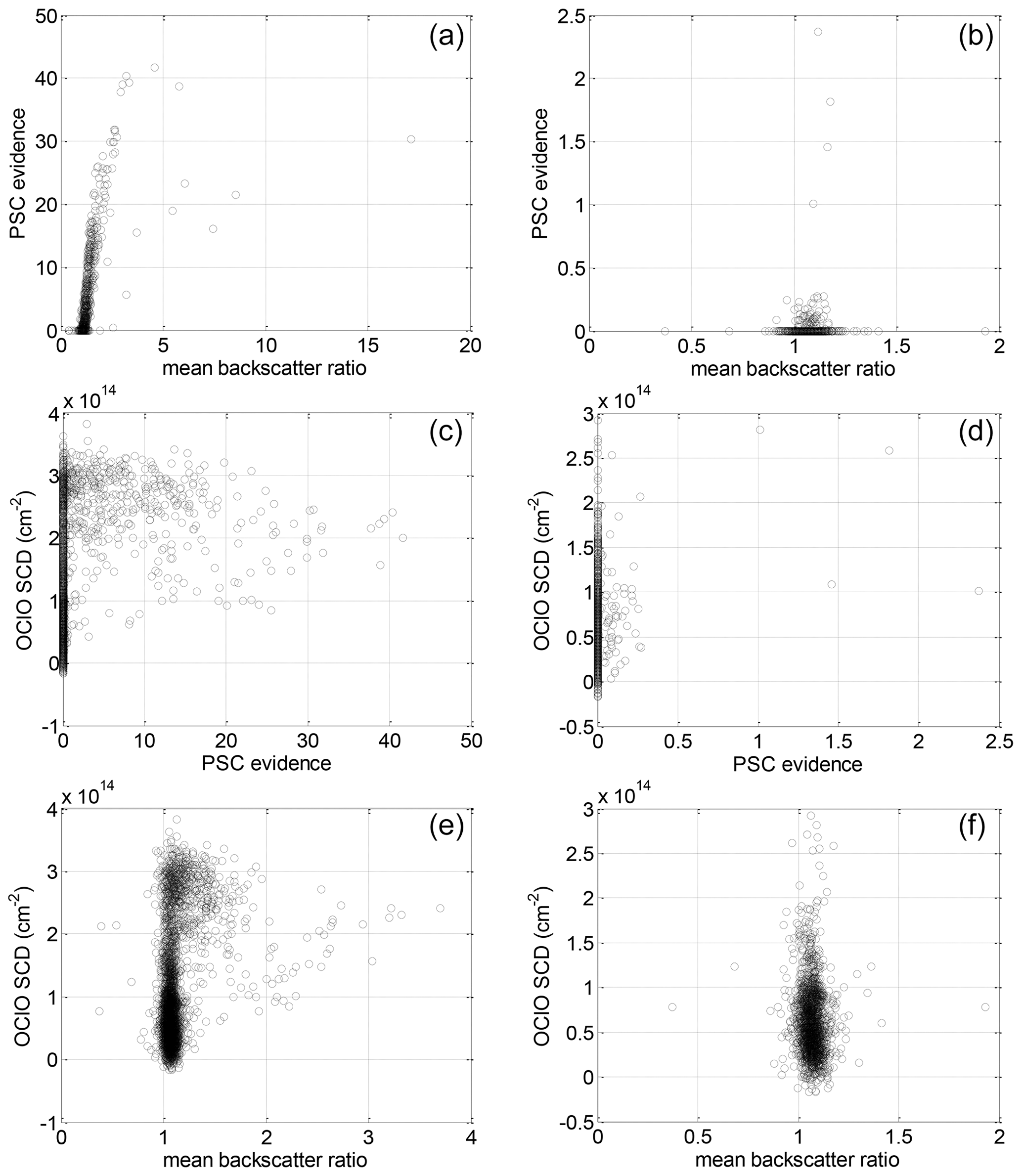
Figure B2 (a, b) Correlation plots between PSC evidence and the mean backscatter ratio. (c, d) Correlation plots between the OClO SCDs and the PSC evidence. (e, f) Correlation plots between the OClO SCDs and the mean backscatter ratio. In panels (a, c, e), data for May–July 2020 are considered, and in panels (b, d, f), just data for May 2020 are included.