Secondary ice production processes in wintertime alpine mixed-phase clouds

Observations of orographic mixed-phase clouds (MPCs) have long shown that measured ice crystal number concentrations (ICNCs) can exceed the concentration of ice nucleating particles by orders of magnitude. Additionally, model simulations of alpine clouds are frequently found to underestimate the amount of ice compared with observations. Surface-based blowing snow, hoar frost, and secondary ice production processes have been suggested as potential causes, but their relative importance and persistence remains highly uncertain. Here we study ice production mechanisms in wintertime orographic MPCs observed during the Cloud and Aerosol Characterization Experiment (CLACE) 2014 campaign at the Jungfraujoch site in the Swiss Alps with the Weather Research and Forecasting model (WRF). Simulations suggest that droplet shattering is not a significant source of ice crystals at this specific location, but breakups upon collisions between ice particles are quite active, elevating the predicted ICNCs by up to 3 orders of magnitude, which is consistent with observations. The initiation of the ice–ice collisional breakup mechanism is primarily associated with the occurrence of seeder–feeder events from higher precipitating cloud layers. The enhanced aggregation of snowflakes is found to drive secondary ice formation in the simulated clouds, the role of which is strengthened when the large hydrometeors interact with the primary ice crystals formed in the feeder cloud. Including a constant source of cloud ice crystals from blowing snow, through the action of the breakup mechanism, can episodically enhance ICNCs. Increases in secondary ice fragment generation can be counterbalanced by enhanced orographic precipitation, which seems to prevent explosive multiplication and cloud dissipation. These findings highlight the importance of secondary ice and seeding mechanisms – primarily falling ice from above and, to a lesser degree, blowing ice from the surface – which frequently enhance primary ice and determine the phase state and properties of MPCs.

1 Introduction

Understanding orographic precipitation is one of the most critical aspects of weather forecasting in mountainous regions (Roe, 2005; Rotunno and Houze, 2007; Chow et al., 2013). Orographic clouds are often mixed-phase clouds (MPCs) containing simultaneously supercooled liquid water droplets and ice crystals (Lloyd et al., 2015; Lohmann et al., 2016; Henneberg et al., 2017). MPCs are persistent in complex mountainous terrain because the high updraft velocity conditions generate supercooled liquid droplets faster than can be depleted by ice production mechanisms (Korolev and Isaac, 2003; Lohmann et al., 2016). In mid- and high-latitude environments, almost all precipitation originates from the ice phase (Field and Heymsfield, 2015; Mülmenstädt et al., 2015), emphasizing the necessity of correctly simulating the amount and distribution of both liquid water and ice (i.e., the liquid-ice-phase partitioning) in MPCs (Korolev et al., 2017).

Our understanding of MPCs remains incomplete, owing to the numerous and highly nonlinear cloud microphysical pathways driving their properties and evolution (Morrison et al., 2012). MPCs tend to glaciate over time through the Wegener–Bergeron–Findeisen (WBF) process, which is the rapid ice crystal growth at the expense of the surrounding evaporating cloud droplets (Bergeron, 1935; Findeisen, 1938). Ice crystals falling from a high-level seeder cloud into a lower-level cloud (external seeder–feeder event) or a lower-lying part of the same cloud (in-cloud seeder–feeder event) can trigger cloud glaciation and enhance precipitation over mountains (e.g., Roe, 2005; Reinking et al., 2000; Purdy et al., 2005; Mott et al., 2014; Ramelli et al., 2021). Analysis of satellite remote sensing over the 11-year period, between April 2006 and October 2017, suggests that seeding events are widespread over Switzerland, occurring with a frequency of 31 % of the total observations in which cirrus clouds seed lower mixed-phase cloud layers (Proske et al., 2021).

Primary ice formation in MPCs is catalyzed by the action of ice nucleating particles (INPs; e.g., Hoose and Möhler, 2012; Kanji et al., 2017). However, in situ observations of MPCs in orographic environments regularly reveal that measured ice crystal number concentrations (ICNCs) are several orders of magnitude more abundant than INPs (Rogers and Vali, 1987; Geerts et al., 2015; Lloyd et al., 2015; Beck et al., 2018; Lowenthal et al., 2019; Mignani et al., 2019). Model simulations of alpine MPCs frequently fail to reproduce the elevated ICNCs dictated by observations (Farrington et al., 2016; Henneberg et al., 2017; Dedekind et al., 2021).

The inability of primary ice to reproduce the observed ICNCs in orographic MPCs has often been attributed to the influence of surface processes, including lofting of snowflakes (i.e., blowing snow; Rogers and Vali, 1987; Geerts et al., 2015), detachment of surface hoar frost (Lloyd et al., 2015), turbulence near the mountain surface or convergence of ice particles due to orographic lifting (Beck et al., 2018), and riming on snow-covered surfaces (Rogers and Vali, 1987). The impact of blowing snow ice particles (BIPs) has been studied thoroughly, either using observations collected in mountainous regions (e.g., Lloyd et al., 2015; Beck et al., 2018; Lowenthal et al., 2019), remote sensing (e.g., Rogers and Vali, 1987; Vali et al., 2012; Geerts et al., 2015), or detailed snow-cover models (e.g., Lehning et al., 2006; Krinner et al., 2018) coupled with atmospheric models (e.g., Vionnet et al., 2014; Sharma et al., 2021). The extent to which BIPs can affect ICNCs in MPCs remains poorly understood.

In-cloud secondary ice production (SIP) – or ice multiplication – processes may also enhance ice production above the concentration of INPs (Field et al., 2017; Korolev and Leisner, 2020). A total of three mechanisms are thought to be responsible for most of the SIP. The first, known as the Hallett–Mossop (HM) process (Hallett and Mossop, 1974), refers to the ejection of small secondary ice splinters after a supercooled droplet with a diameter larger than ∼ 25 µm rimes onto a large ice particle at temperatures between −8 and −3 ^∘C (Choularton et al., 1980; Heymsfield and Mossop, 1984). This SIP mechanism is widely implemented in atmospheric models (e.g., Beheng, 1987; Phillips et al., 2001; Morrison et al., 2005) but cannot, on its own, explain the enhanced ICNCs in remote environments (Young et al., 2019; Sotiropoulou et al., 2020, 2021a), especially for when the conditions required for HM initiation are not fulfilled (e.g., Korolev et al., 2020).

Collisional fracturing and breakup (BR) of delicate ice particles with other ice particles (Vardiman, 1978; Griggs and Choularton, 1986; Takahashi et al., 1995) is another important SIP mechanism. Several field studies in the Arctic (Rangno and Hobbs, 2001; Schwarzenboeck et al., 2009), the Alps (Mignani et al., 2019; Ramelli et al., 2021), and laboratory investigations (Vardiman 1978; Takahashi et al. 1995) all show the importance of BR. The latter two studies created the basis for a mechanistic description of BR (e.g., Phillips et al., 2017a; Sullivan et al., 2018a; Sotiropoulou et al., 2020). Parameterizations of BR have recently been implemented in small-scale (Fridlind et al., 2007; Phillips et al., 2017a, b; Sotiropoulou et al., 2020, 2021b; Sullivan et al., 2018a; Yano and Phillips, 2011; Yano et al., 2016), mesoscale (Hoarau et al., 2018; Sullivan et al., 2018b; Qu et al., 2020; Sotiropoulou et al., 2021a; Dedekind et al., 2021), and global climate models (Zhao and Liu, 2021a), each with their own approach towards BR description.

Droplet freezing and shattering (DS) is a third SIP mechanism that can produce significant amounts of ice crystals. It occurs when drizzle-sized drops (diameter exceeding 50 µm) come in contact with an ice particle or INP. A solid ice shell is initially formed around the droplet (e.g., Griggs and Choularton, 1983), and as it thickens, it begins building up pressure that leads to a breakup in two halves, cracking, bubble burst, or jetting (e.g., Keinert et al., 2020). The ejection of small ice fragments may occur, the number of which varies considerably (Lauber et al., 2018; Keinert et al., 2020; Kleinheins et al., 2021; James et al., 2021). Experimentally, the fragmentation rate maximizes at temperatures between $\sim -\mathrm{10}$ and −15 ^∘C (Leisner et al., 2014; Lauber et al., 2018; Keinert et al., 2020). DS can dominate in convective updrafts (Lawson et al., 2015; Phillips et al., 2018; Korolev et al., 2020; Qu et al., 2020). Remote sensing of warm Arctic MPCs suggests DS can be much more conducive to SIP than the HM process (Luke et al., 2021). Single-column simulations by Zhao et al. (2021) support this but are in contrast with small-scale modeling studies (Fu et al., 2019; Sotiropoulou et al., 2020). Mesoscale model simulations of winter alpine clouds formed at temperatures lower than −8 ^∘C indicate that DS is not active (Dedekind et al., 2021), while field observations suggest the increasing efficiency of the mechanism at temperatures warmer than −3 ^∘C (Lauber et al., 2021).

Orographic ICNCs in MPCs exceeded the predicted INPs by 3 orders of magnitude, reaching up to ∼ 1000 L⁻¹ at −15 ^∘C during the Cloud and Aerosol Characterization Experiment (CLACE) 2014 campaign at the Jungfraujoch (JFJ) station in the Swiss Alps (Lloyd et al., 2015). Although the efficiency of BR and DS peaks at around the same temperature, Lloyd et al. (2015) did not find evidence for their occurrence. Instead, at periods when there was a strong correlation between horizontal wind speed and observed ICNC they suggested that BIPs are contributing to the latter but could not make ICNCs exceed ∼ 100 L⁻¹. In the absence of such a correlation, a flux of hoar frost crystals was considered to be responsible for the very high ice concentration events (ICNCs > 100 L⁻¹), albeit without any direct evidence. Farrington et al. (2016) showed that the inclusion of the HM process upwind of JFJ could not explain the measured concentrations of ice, while the addition of a surface flux of hoar crystals provided the best agreement with observations.

Although surface-originated processes have been frequently invoked to explain the disparity between ICNCs and INPs, the role of SIP processes – especially the BR and the DS mechanism – has received far less attention and is addressed in this study. We utilize the Weather Research and Forecasting model (WRF) to conduct simulations of two case studies observed in winter during the CLACE 2014 campaign. Our primary objective is to investigate if the implementation of two SIP parameterizations that account for the effect of BR and DS can reduce the discrepancies between observed and simulated ICNCs. Additionally, we aim to identify the conditions favoring the initiation of SIP in the orographic terrain and explore the synergistic influence of SIP with windblown ice.

2 Methods

2.1 CLACE instrumentation

CLACE is a long-established series of campaigns taking place for over 2 decades at the mountain-top station of JFJ, located in the Bernese Alps, in Switzerland, at an altitude of ∼ 3580 m above sea level (a.s.l.; e.g., Choularton et al., 2008). The measurement area is very complex and heterogeneous with distinct mountain peaks (Fig. 1), while JFJ is covered by clouds approximately 40 % of the time, offering an ideal location for microphysical observations (Baltensperger et al., 1998). Owing to the local orography surrounding the site, the wind flow is constrained to two directions (Ketterer et al., 2014). Under southeasterly (SE) wind conditions, air masses are lifted along the moderate slope of the Aletsch Glacier, whereas under northwesterly (NW) wind conditions, the air is forced to rise faster along the steep northern face of the Alps, which is associated with persistent MPCs (Lohmann et al., 2016). A detailed description of the in situ and remote sensing measurements taken during January and February 2014, as part of the CLACE 2014 campaign, is provided by Lloyd et al. (2015) and Grazioli et al. (2015). Here we only offer a brief presentation of the datasets used in this study.

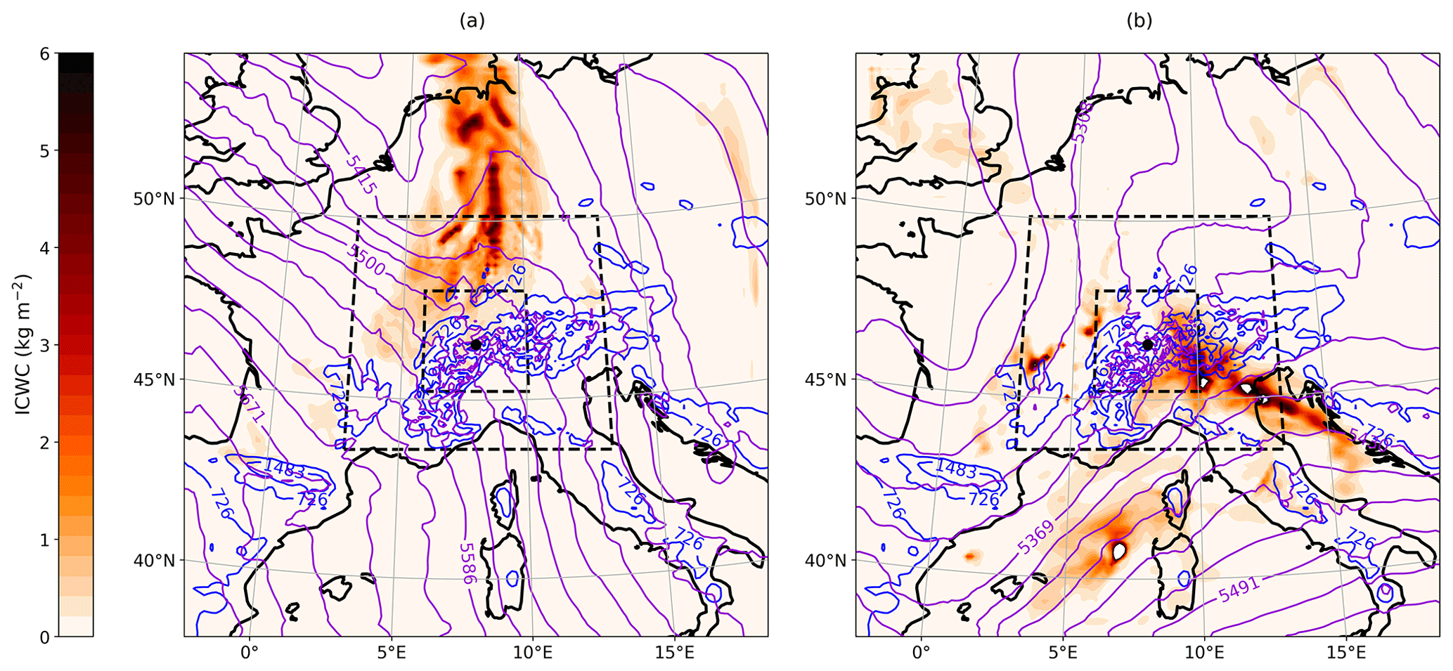
Figure 1 Map of synoptic conditions around JFJ station at (a) 00:00 UTC, 26 January 2014, and (b) 00:00 UTC, 30 January 2014, from the control simulation (12 km resolution domain). The purple (blue) contours show the 500 hPa geopotential height in meters (the terrain heights in meters). The color shading shows the vertically integrated condensed water content (in kilograms per square meter; hereafter kg m⁻²). The black dashed lines delimit the 3 and 1 km resolution domains, while the black dot indicates the location of the JFJ station.

Shadowgraphs of cloud particles were produced by the two-dimensional stereo hydrometeor spectrometer (2D-S; Lawson et al., 2006), part of a three-view cloud particle imager (3V-CPI) instrument. The 2D-S products have been used to provide information on the number concentration and size distribution of particles in the size range of 10–1280 µm. Following Crosier et al. (2011), the raw data were processed to distinguish ice crystals from droplets. Removal of artifacts from shattering events was also considered (Korolev et al., 2011); however, analysis of the probe imagery (Crosier et al., 2011), along with interarrival time histograms, did not reveal the presence of shattered particles, presumably because of the much lower velocity at which the 2D-S probe was aspirated (∼ 15 ms⁻¹) compared to those during aircraft deployments (Lloyd et al., 2015). An approximation of the ice water content (IWC) at JFJ could also be derived by the 2D-S data using the Brown and Francis (1995) mass–diameter relationship with an uncertainty of up to 5 times (Heymsfield et al., 2010). Additionally, the quantification of the liquid water content (LWC) is based on the liquid droplet size distribution data derived from a DMT (Droplet Measurement Technologies, Inc.) cloud droplet probe (CDP; Lance et al., 2010) over the size range between 2 and 50 µm. Meteorological parameters (e.g., temperature, relative humidity, wind speed, and wind direction) were provided by MeteoSwiss and used to evaluate the model.

2.2 WRF simulations

WRF version 4.0.1, with augmented cloud microphysics to include the effects of additional SIP mechanisms (Sotiropoulou et al., 2021a) is used for non-hydrostatic cloud-resolving simulations. The model has been run with three two-way nested domains (Fig. 1), with a respective horizontal resolution of 12, 3, and 1 km. A two-way grid nesting is generally found to improve the model performance in the inner domain (e.g., Harris and Durran, 2010), although the sensitivity of the results to the applied nesting technique has been shown to be negligible (not shown). The parent domain consists of 148 × 148 grid points centered over the JFJ station (46.55^∘ N, 7.98^∘ E; shown as a black dot in Fig. 1), while the second and the third domain include 241 × 241 and 304 × 304 grids, respectively. The Lambert conformal projection is applied to all three domains, as it is well suited to mid-latitudes. Here we adapted the so-called refined vertical grid spacing proposed by Vignon et al. (2021), using 100 vertical eta levels up to a model top of 50 hPa (i.e., ∼ 20 km). This setup provides a refined vertical resolution of ∼ 100 m up to mid-troposphere at the expense of the coarsely resolved stratosphere. To investigate the dynamical influence on the development of MPCs under the two distinct wind regimes prevailing at JFJ (Sect. 2.1), we simulate two case studies, starting on 25 and 29 January 2014, 00:00 UTC, respectively. Both case studies are associated with the passage of frontal systems over the region of interest, approaching the alpine slopes either from the NW (cold front) or the SE (warm front) direction, as shown by the vertically integrated condensed water content (ICWC; sum of cloud droplets, rain, cloud ice, snow, and graupel) in Fig. 1. For both cases, the simulation covers a 3 d period, with the first 24 h being considered sufficient time for the spin-up. A 27 s time step was used in the parent domain and goes down to 9 s in the second domain and 3 s in the third domain. Note that achieving such small time steps in the innermost domain is essential to ensure numerical stability in non-hydrostatic simulations over a region with complex orography such as around JFJ.

The fifth generation of the European Centre for Medium-Range Weather Forecasts (ECMWF) atmospheric reanalyses dataset (ERA5; Hersbach et al., 2020) is used to initialize the model and provide the lateral forcing at the edge of the 12 km resolution domain every 6 h. Static fields at each model grid point come from default WRF pre-processing system datasets, with a resolution of 30^′′ for both the topography and the land use fields. Land use categories are based on the Moderate Resolution Imaging Spectroradiometer (MODIS) land cover classification. Regarding the physics options chosen to run WRF simulations, the Rapid Radiative Transfer Model for General Circulation Models (RRTMG) radiation scheme is applied to parameterize both the short-wave and long-wave radiative transfer. The vertical turbulent mixing is treated with the Mellor–Yamada–Janjić (MYJ; Janjić, 2001) 1.5 order scheme, while surface options are modeled by the Noah land surface model (Noah LSM; Chen and Dudhia, 2001). The Kain–Fritsch cumulus parameterization has been activated only in the outermost domain, as the resolution of the two nested domains is sufficient to reasonably resolve cumulus-type clouds at grid scale.

2.2.1 Microphysics scheme and primary ice production

The Morrison two-moment scheme (Morrison et al., 2005; hereafter M05) is used to parameterize the cloud microphysics, following the alpine cloud study of Farrington et al. (2016). The scheme includes double-moment representations of rain, cloud ice, snow, and graupel species, while cloud droplets are treated with a single-moment approach, and therefore, the cloud droplet number concentration (N_d) must be prescribed. Here N_d is set to 100 cm⁻³, based on the mean N_d observed within the simulated temperature range (Lloyd et al., 2015).

In total, three primary ice production mechanisms through heterogeneous nucleation are described in the default version of the M05 scheme, namely immersion freezing, contact freezing, and deposition/condensation freezing nucleation. Immersion freezing of cloud droplets and raindrops is described by the probabilistic approach of Bigg (1953). Contact freezing is parameterized following Meyers et al. (1992). Finally, deposition and condensation freezing is represented by the temperature-dependent equation derived by Rasmussen et al. (2002), based on the in situ measurements of Cooper (1986) collected from different locations at different temperatures. Following Thompson et al. (2004), this parameterization is activated either when there is saturation with respect to liquid water and the simulated temperatures are below −8 ^∘C or when the saturation ratio with respect to ice exceeds a value of 1.08. The accuracy of these parameterizations in representing atmospheric INPs is debatable, as they are derived from very localized measurements over a limited temperature range. Nevertheless, Farrington et al. (2016) argued that the deposition/condensation freezing parameterization of Cooper (1986) can effectively explain INPs between the range 0.01 and 10 L⁻¹, which is frequently observed during field campaigns at JFJ (Chou et al., 2011; Conen et al., 2015).

2.2.2 Ice multiplication through rime splintering in the M05 scheme

Apart from primary ice production, the HM process is the only SIP mechanism included in the default version of the M05 scheme. This parameterization adapted from Reisner et al. (1998), based on the laboratory findings of Hallett and Mossop (1974), allows for splinter production after cloud- or raindrops are collected by rimed snow particles or graupel. The efficiency of this process is zero outside the temperature range between −8 and −3 ^∘C, while it follows a linear temperature-dependent relationship in between. HM is not activated unless the rimed ice particles have masses larger than 0.1 g kg⁻¹ and cloud or rain mass mixing ratio exceeds the value of 0.5 or 0.1 g kg⁻¹, respectively. Since these conditions are rarely met in natural MPCs, previous modeling studies had to artificially remove any thresholds to achieve an enhanced efficiency of this process (Young et al., 2019; Atlas et al., 2020). In the current study, however, the HM process is not effective, as the simulated temperatures at JFJ altitude are below −8 ^∘C (see Sect. 2.3).

2.2.3 Ice multiplication through ice–ice collisions in the M05 scheme

In addition to the HM process, we have also included two parameterizations to represent the BR mechanism. An extensive description of the implementation method is provided in Sotiropoulou et al. (2021a; see their Appendix B). Among the three ice particle types included in the M05 scheme (i.e., cloud ice, snow, and graupel), we assume that only the collisions between cloud ice–snow, cloud ice–graupel, graupel–snow, snow–snow, and graupel–graupel can result in ice multiplication. The first parameterization tested here follows the simplified methodology proposed by Sullivan et al. (2018a), which is based on the laboratory work of Takahashi et al. (1995). Their findings revealed a strong temperature dependence of the fragment numbers generated per collision (N_BR), as follows:

$$\begin{array}{}\text{(1)}& N_{\mathrm{BR}}=\mathrm{280}(T-T_{\min }{)}^{\mathrm{1.2}}{e}^{-(T-T_{\min })/\mathrm{5}},\end{array}$$

where T_min=252 K, is the minimum temperature for which BR occurs. Yet, their experimental setup was rather simplified, involving only collisions between large hail-sized ice spheres with diameters of ∼ 2 cm. Taking this into account, Sotiropoulou et al. (2021a) further scaled the temperature-dependent formulation for size as follows:

$$\begin{array}{}\text{(2)}& N_{\mathrm{BR}}=\mathrm{280}(T-T_{\min }{)}^{\mathrm{1.2}}{e}^{-(T-T_{\min })/\mathrm{5}}{\displaystyle \frac{D}{D_{\mathrm{0}}}},\end{array}$$

where D is the size in meters of the particle that undergoes breakup and D₀= 0.02 m is the size of the hail-sized balls used in the experiments of Takahashi et al. (1995).

Phillips et al. (2017a) proposed a more physically based formulation, developing an energy-based interpretation of the experimental results conducted by Vardiman (1978) and Takahashi et al. (1995). The initial collisional kinetic energy is considered as being the governing constraint driving the BR process. Moreover, the predicted N_BR depends on the ice particle type and morphological habit and is a function of the temperature, particle size, and rimed fraction. Here the generated fragments per collision are described as follows:

$$\begin{array}{}\text{(3)}& N_{\mathrm{BR}}=aA\left(\mathrm{1}-\exp \left\{-{\left[{\displaystyle \frac{C{K}_{\mathrm{0}}}{aA}}\right]}^{\mathit{\gamma }}\right\}\right),\end{array}$$

where $K_{\mathrm{0}}=\frac{\mathrm{1}}{\mathrm{2}}\frac{m_{\mathrm{1}}{m}_{\mathrm{2}}}{m_{\mathrm{1}}+m_{\mathrm{2}}}{\left(\mathrm{\Delta }{u}_{n\mathrm{12}}\right)}^{\mathrm{2}}$ is the initial kinetic energy in which m₁ and m₂ are the masses of the colliding particles, and $\left|\mathrm{\Delta }{u}_{n\mathrm{12}}\right|={\left\{{\left(\mathrm{1.7}{u}_{n\mathrm{1}}-u_{n\mathrm{2}}\right)}^{\mathrm{2}}+\mathrm{0.3}{u}_{n\mathrm{1}}{u}_{n\mathrm{2}}\right\}}^{\mathrm{1}/\mathrm{2}}$ is the difference in their terminal velocities. The correction term is proposed by Mizuno et al. (1990) and Reisner et al. (1998) to account for underestimates when u_n1≈u_n2. The parameter a in Eq. (3) is the surface area of the smaller ice particle (or the one with the lower density), defined as a=πD², with D as in Eq. (2). A in Eq. (3) represents the number density of breakable asperities on the colliding surfaces. For collisions that involve cloud ice and snow particles, A is described as $A=\mathrm{1.58}\times {\mathrm{10}}^{\mathrm{7}}(\mathrm{1}+\mathrm{100}{\mathrm{\Psi }}^{\mathrm{2}})\left(\mathrm{1}+\frac{\mathrm{1.33}\times {\mathrm{10}}^{-\mathrm{4}}}{D^{\mathrm{1.5}}}\right)$, where Ψ < 0.5 is the rimed fraction of the most fragile ice particle. For graupel–graupel collisions, A is given by a temperature-dependent equation as $A=\frac{a_{\mathrm{0}}}{\mathrm{3}}+\max \left(\frac{\mathrm{2}{a}_{\mathrm{0}}}{\mathrm{3}}-\frac{a_{\mathrm{0}}}{\mathrm{9}}\left|T-\mathrm{258}\right|,\mathrm{0}\right)$, in which $a_{\mathrm{0}}=\mathrm{3.78}\times {\mathrm{10}}^{\mathrm{4}}\left(\mathrm{1}+\frac{\mathrm{0.0079}}{D^{\mathrm{1.5}}}\right)$. C is the asperity–fragility coefficient, which is empirically derived to account for different collision types, while the exponent γ is equal to 0.3 for collisions between graupel–graupel and is calculated as a function of the rimed fraction for collisions including cloud ice and snow. The parameterization was developed based on particles with diameters 500 µm < D < 5 mm; however, Phillips et al. (2017a) suggest that it can be used for particle sizes outside the recommended range as long as the input variables to the scheme are set to the nearest limit of the range. Finally, since N_BR was never observed to exceed 100 in the experiments of Vardiman (1978), here we also use this value as an upper limit for all collision types (Phillips et al., 2017a). All predicted fragments emitted through BR are added to the cloud ice category.

2.2.4 Ice multiplication through droplet shattering in the M05 scheme

In the M05 scheme, two different parameterizations are implemented to investigate the potential efficiency of the DS mechanism in producing secondary ice splinters (N_DS). Phillips et al. (2018) proposed two possible modes of raindrop–ice collisions that can initiate the freezing process. In the first mode, the freezing of the drop occurs either by collecting a small ice particle or through heterogeneous freezing. In the default M05 scheme, the product of collisions between raindrops and cloud ice is considered to be graupel (snow) if the rain mixing ratio is greater (lower) than 0.1 g kg⁻¹, following Reisner et al. (1998). Additionally, the heterogeneous freezing of big raindrops in the immersion mode follows Bigg's (1953) parameterization (Sect. 2.2.1). Here we consider that the product of these two processes can undergo shattering and generate numerous ice fragments, the number of which is parameterized after Phillips et al. (2018). The formulation is derived by fitting multiple laboratory datasets to a Lorentzian function of temperature and a polynomial expression of the drop size. More precisely, the total number of fragments (N) generated per frozen drop are given by the following:

$$\begin{array}{}\text{(4)}& N=\mathrm{\Xi }\left(D_{\mathrm{r}}\right)\mathrm{\Omega }\left(T\right)\left[{\displaystyle \frac{\mathit{\zeta }{\mathit{\eta }}^{\mathrm{2}}}{(T-T_{\mathrm{0}}{)}^{\mathrm{2}}+{\mathit{\eta }}^{\mathrm{2}}}}+\mathit{\beta }T\right],\end{array}$$

where T is the temperature (in Kelvin), and D_r is the size of the freezing raindrop (in millimeters). Note that N is defined as the sum of the big fragments (N_B) and tiny splinters (N_T). Equation (4) applies only to drop diameters less than 1.6 mm, which is the maximum observed experimentally. For droplet sizes beyond this maximum value, N can be inferred by linear extrapolation. N_B is described by another Lorentzian as follows:

$$\begin{array}{}\text{(5)}& N_{\mathrm{B}}=min\left\{\mathrm{\Xi }\left(D_{\mathrm{r}}\right)\mathrm{\Omega }\left(T\right)\left[{\displaystyle \frac{{\mathit{\zeta }}_{\mathrm{B}}{\mathit{\eta }}_{\mathrm{B}}^{\mathrm{2}}}{{\left(T-T_{B,\mathrm{0}}\right)}^{\mathrm{2}}+{\mathit{\eta }}_{\mathrm{B}}^{\mathrm{2}}}}\right],N\right\}.\end{array}$$

The factors Ξ(D_r) and Ω(T) in Eqs. (4) and (5) are cubic interpolation functions, impeding DS for D_r < 0.05 mm and T > −3 ^∘C. Furthermore, the parameters ζ, η, T₀, β, ζ_B, η_B, and T_B,0 are analytically described in Phillips et al. (2018). Note that the big fragments emitted (i.e., N_B) will be initiated in the model as graupel, snow, or frozen drops, while only the tiny splinters ($N_{\mathrm{T}}=N-N_{\mathrm{B}}$) are considered secondary ice (i.e., N_DS=N_T) and are passed to the cloud ice category.

The second mode of raindrop–ice collisions includes the accretion of raindrops on impact with more massive ice particles, such as snow or graupel, the description of which in the M05 scheme is adapted from Ikawa and Saito (1991). While there is only one dedicated laboratory study of this SIP mode (James et al., 2021), it was also indirectly investigated in the experimental study of Latham and Warwicker (1980), who reported that the collision of supercooled raindrops with hailstones can generate secondary ice. Phillips et al. (2018) proposed an empirical, energy-based formulation to account for the tiny splinters ejected after collisions between raindrops and large ice particles as follows:

$$\begin{array}{}\text{(6)}& N_{\mathrm{DS}}=\mathrm{3}\mathrm{\Phi }\left(T\right)\times \left[\mathrm{1}-f\left(T\right)\right]\times max\left(\mathrm{DE}-{\mathrm{DE}}_{\mathrm{crit}},\mathrm{0}\right),\end{array}$$

where DE $=\frac{K_{\mathrm{0}}}{S_{\mathrm{e}}}$ is the dimensionless energy given as the ratio of the initial kinetic energy (K₀; described in Sect. 2.2.3) over the surface energy, which is expressed by the product $S_{\mathrm{e}}={\mathit{\gamma }}_{\mathrm{liq}}\mathit{\pi }{D}_{\mathrm{r}}^{\mathrm{2}}$, in which γ_liq= 0.073 J m⁻² is the surface tension of liquid water. The critical value of DE used in Eq. (6) for the onset of splashing upon impact is set to DE_crit= 0.2. The parameter $f\left(T\right)=-c_{\mathrm{w}}T/L_{\mathrm{f}}$ represents the initial frozen fraction of a supercooled drop during the first stage of the freezing process, where c_w= 4200 J kg⁻¹ K⁻¹ is the specific heat capacity of liquid water, and L_f= 3.3 × 10⁵ J kg⁻¹ is the specific latent heat of freezing, while T is the initial freezing temperature (degrees Celsius) of the raindrop. Finally, Φ(T)= min[4f(T),1] is an empirical fraction which represents the probability of any new drop in the splash products to contain a frost secondary ice particle. At temperatures ∼ −10 ^∘C, this formulation yields Φ= 0.5, meaning that the probability of a secondary drop containing ice is 50 %. James et al. (2021) provided the first laboratory study to constrain this parameter. Further details regarding the derivation of the empirical parameters and the uncertainties underlying the mathematical formulations are discussed in Phillips et al. (2018).

The second DS parameterization tested in this study was developed by Sullivan et al. (2018a) and is a function of the freezing droplet diameter (D_r in µm), a shattering probability (p_sh), and a freezing probability (p_fr) as follows:

$$\begin{array}{}\text{(7)}& N_{\mathrm{DS}}=\mathrm{2.5}\times {\mathrm{10}}^{-\mathrm{11}}{D}_{\mathrm{r}}^{\mathrm{4}}{p}_{\mathrm{sh}}{p}_{\mathrm{fr}}.\end{array}$$

The diameter dependence describing the fragment numbers generated per fractured frozen droplet is derived by nudging the liquid water and ice particle size distributions in one-dimensional cloud model simulations towards aircraft observations collected in tropical cumulus clouds (Lawson et al., 2015). The p_sh is based upon droplet levitation experiments shown in Leisner et al. (2014) and is represented by a temperature-dependent Gaussian distribution, centered at ∼ −15 ^∘C. Note that p_sh is non-zero only for droplets with sizes greater than 50 µm. The p_fr is 0 for temperatures warmer than −3 ^∘C and 1 if temperatures fall below −6 ^∘C, following the cubic interpolation function, Ω(T), adapted from Phillips et al. (2018).

2.3 Model evaluation

The control simulation (CNTRL), performed with the standard M05 scheme, sets the basis for assessing the validity of the model against available meteorological observations. Temperature, relative humidity, wind speed, and wind direction are obtained from the MeteoSwiss weather station at JFJ. The comparison of each meteorological variable with the results from the nearest model grid point of the CNTRL simulation is shown in Fig. 2. Note that the outputs are from the first atmospheric level of the innermost domain at ∼ 10 m above ground level (a.g.l.; Fig. 1), while the first 24 h of each simulation period are considered spin-up time and are, therefore, excluded from the present analysis. The mean modeled values and standard deviations (SDs), along with the root mean square error (RMSE), and the index of agreement (IoA) between model predictions and observational data are summarized in Table 1. IoA is both a relative and a bounded measure (i.e., 0 ≤ IoA ≤ 1) that describes phase errors between predicted (P_i) and observed (O_i) time series (Willmott et al., 2012) as follows:

$$\begin{array}{}\text{(8)}& \mathrm{IoA}=\mathrm{1}-\left[{\displaystyle \frac{{\sum }_{i=\mathrm{1}}^N(P_i-O_i{)}^{\mathrm{2}}}{{\sum }_{i=\mathrm{1}}^N(\left|P_i^{\prime }\right|-\left|O_i^{\prime }\right|{)}^{\mathrm{2}}}}\right],\end{array}$$

where ${P^{\prime }}_i=P_i-\stackrel{\mathrm{‾}}{O}$ and ${O^{\prime }}_i=O_i-\stackrel{\mathrm{‾}}{O}$, in which $\stackrel{\mathrm{‾}}{O}$ is the mean of the observed variable.

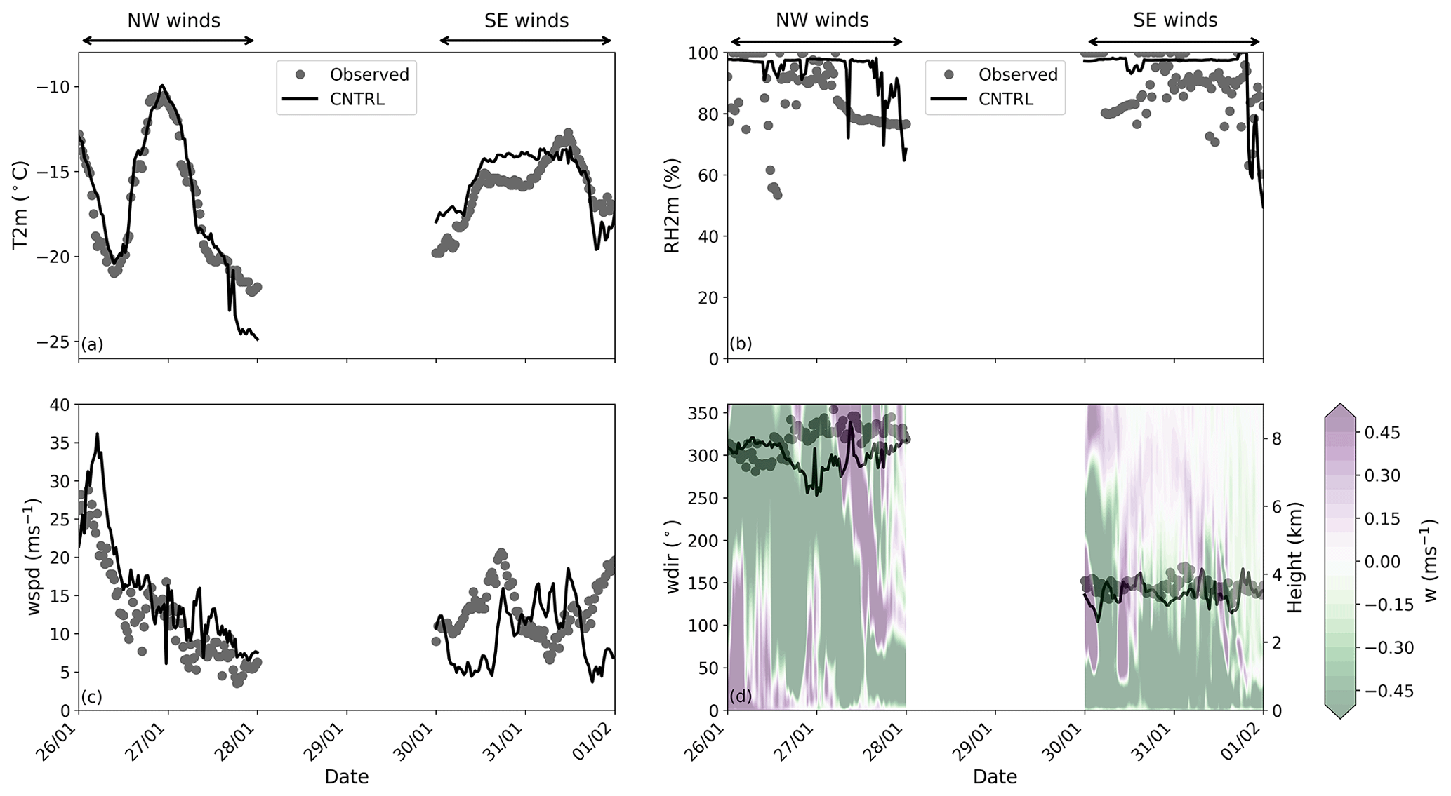
Figure 2 Time series of (a) temperature (T2m), (b) relative humidity with respect to liquid phase at 2 m height (RH2m), (c) wind speed (wspd), and (d) wind direction (wdir). Gray circles indicate measurements collected between 26 January and 1 February 2014 at JFJ station, while modeled values from the CNTRL simulation are shown with a black line. The semi-transparent contour plot represents the vertical velocity (w) profile predicted by the CNTRL simulation. Each day starts at 00:00 UTC.

Throughout the two case studies, the WRF simulations seem to closely follow the observed temperatures (Fig. 2a), which is also indicated by the high IoA in Table 1. The synoptic situation occurring on 26 January, with a deep trough extending to western Europe (Fig. 1), has been associated with intense snowfall in the alpine regions (Panziera and Hoskins, 2008). The passage of the cold front was followed by a sharp temperature decrease, with the simulated temperatures fluctuating between −10 and ∼ −20 ^∘C throughout the NW case (Fig. 2a). Under the influence of the warm front during the SE case, the modeled temperatures rose from ∼ −18 to ∼ −14 ^∘C and remained less variable until 30 January at 12:00 UTC, with mean values of ∼ −15.5 ^∘C (Table 1).

Table 1 Mean modeled values (± SDs), RMSE, and IoA between the CNTRL simulation of WRF and measurements carried out by the MeteoSwiss station at JFJ.

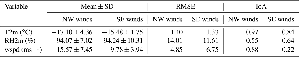
The 1 km resolution domain can sufficiently capture the local wind systems to a certain extent (Fig. 2c, d). During the NW flow, the horizontal wind speeds are reproduced better by the CNTRL simulation (IoA = 88 %), whereas during the SE winds, the simulated wind speed is frequently underestimated compared with observations (Fig. 2c). Such deviations in the horizontal wind speed might be caused by the relatively coarse horizontal resolution of the model, which prevents some small-scale and very local orographic structures from being resolved. As discussed in Sect. 2.2, the observed winds at JFJ are channeled by the orography to either NW or SE directions. The CNTRL simulation of WRF can satisfactorily reproduce the wind direction in both cases, although the simulated values exhibit larger fluctuations than the measured ones (Fig. 2d), presumably because of the surrounding orography being less accurately represented in the model. This is particularly evident during NW winds, when the simulated wind directions shift slightly to west directions compared to observations. The positive vertical velocities, illustrated in the contour plot in Fig. 2d, result from the orographically forced lifting of the air masses over the local topography and are not related to convective instability in the lower atmospheric levels. The stronger updrafts prevailing until the end of 26 January are associated with the steep ascent of the air parcels, which can also contribute to the enhanced relative humidity (Fig. 2b). After the frontal passage, the vertical velocities at the lower levels are downward directed, with the vertical profile of potential temperature revealing that the atmosphere at JFJ is stabilized (not shown). The same vertical velocity pattern, with mainly downward motions, characterizes the stably stratified atmosphere after 30 January. Overall, Fig. 2 suggests that local meteorological conditions at JFJ are reasonably well represented by the model.

2.4 Model simulations

Given the good representation of the atmospheric conditions at JFJ, the CNTRL simulation of WRF is further accompanied by five sensitivity simulations aiming to investigate the contribution of BR and DS mechanisms. Here we also perform three additional sensitivity experiments to explore the potential impact of blowing ice and the synergistic interaction with SIP on the development of the simulated MPCs. A detailed list of the sensitivity experiments is provided in Table 2.

The contribution of the DS mechanism is addressed in two sensitivity experiments, DS_PHILL and DS_SULL, where the parameterizations of Phillips et al. (2018) and Sullivan et al. (2018a) were applied, respectively (Sect. 2.2.4). Both sensitivity simulations yield predictions that coincide with the CNTRL simulation (see Fig. S1 in the Supplement), suggesting that the DS mechanism is hardly ever activated, and fail to produce realistic total ice number concentrations (N_isg; cloud ice + snow + graupel). The absence of correlation between LWC and N_isg fluctuations might also suggest the ineffectiveness of this mechanism under the examined conditions. Note that the parameterized expressions used to describe the DS mechanism involve a number of empirical and rather uncertain parameters, the value of which could potentially influence the efficiency of the process in producing secondary ice fragments. However, the sensitivity of our results to the choice of these parameters would be negligible, as the low concentrations (≲ 10⁻² cm⁻³) of relatively small raindrops with mode diameters below the threshold size of 50 µm seem to completely prevent the onset of the DS process (Fig. S2). The DS mechanism is, therefore, excluded from the following discussion. This result is in line with the modeling study of Dedekind et al. (2021), who also reported the inefficiency of this mechanism in wintertime alpine clouds.

The effect of secondarily formed ice particles through BR is then examined in the following three sensitivity simulations. First, the TAKAH simulation adopts the temperature-dependent formula of Takahashi et al. (1995) scaled with the size of particles that undergo fragmentation (Sotiropoulou et al. 2021a). Applying Eq. (2) to collisions between all ice categories considered in the M05 scheme (except collisions between cloud ice particles; Sect. 2.2.3) inserts a caveat to our approach. The laboratory results of Takahashi et al. (1995) suggest that it is mostly the collisions between rimed particles and graupel that are more conducive to SIP through BR. Vardiman (1978) also reported that ice crystal growth through riming is essential to boost fragmentation. Applying the Takahashi breakup scheme for unrimed ice particles might, therefore, overestimate the number of secondary ice fragments. To test this hypothesis, we performed the TAKAHrim sensitivity simulation, where we enabled ice multiplication through BR only after collisions between rimed cloud ice/snow and graupel particles. To diagnose the presence of rime on ice particles, we used the amount of cloud droplets or raindrops accreted by snow and cloud ice, which is predicted in the M05 scheme.

Table 2 List of sensitivity simulations conducted with WRF. Note: NBIPs is the number concentrations of BIPs.

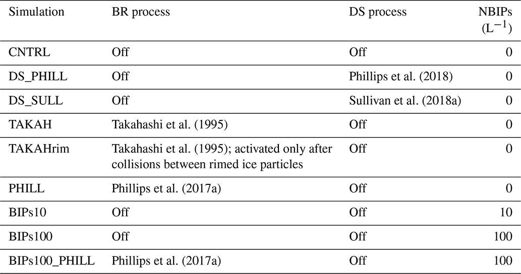
Finally, the performance of the more advanced Phillips et al. (2017a) parameterization is tested in the PHILL simulation. Parameters involved in the Phillips parameterization that are not explicitly resolved in the M05 microphysics scheme are the rimed fraction and the ice habit of colliding ice particles. The choice of ice habit is based on particle images collected during the CLACE 2014 campaign, showing the presence of non-dendritic sectored plates and oblate particles at temperatures ∼ −15 ^∘C (Lloyd et al., 2015). Grazioli et al. (2015) also presented some examples of particle imagery produced by a 2D-S imaging probe, revealing the presence of heavily rimed hydrometeors and highly oblate particles (probably columns or needles). The rimed fraction is prescribed to a value of 0.4 (0.3) to account, respectively, for heavily and moderately rimed ice particles present under NW (SE) wind conditions. A high degree of riming is expected in the simulated cases, as they both occur under ice-seeding situations (Sect. 3.1.1), where large precipitating ice particles from the seeder clouds effectively gain mass in the mixed-phase zone through riming. Direct observations with balloon-borne measurements carried out within ice-seeding events in the region around Davos in the Swiss Alps support the presence of a large fraction of rimed particles and graupel (Ramelli et al., 2021). The higher riming degree is prescribed under NW winds because the orographic forcing (i.e., vertical velocity) is stronger and helps with maintaining mixed-phase conditions in the feeder clouds – which, in turn, promotes ice crystal growth through riming. However, our results were not very sensitive to the choice of the rimed fraction.

The remaining sensitivity simulations focus on the potential impact of BIPs. A recently developed blowing snow scheme, used to simulate alpine snowpacks, reported significant mass and number mixing ratios of BIPs that can be found up to ∼ 1 km above the surface under high wind speed conditions (see Fig. 17 in Sharma et al., 2021), with the potential to trigger cloud microphysical processes. Given that in the default M05 scheme there is no parameterization of a flux of ice particles from the surface, we parameterize the effect of BIPs lofting into the simulated orographic clouds by applying a constant ice crystal source to the first atmospheric level of WRF over the whole model domain. Although the source of BIPs at the first model level remained constant, their number will be affected by processes such as advection, sublimation, and sedimentation that are described in the M05 scheme. Note that the relatively coarse horizontal resolution in the innermost domain of our simulations (i.e., 1 km) does not allow the accurate representation of the small-scale turbulent flow over the orographic terrain. This is considered a limitation of our methodology, since turbulent diffusion is a key process affecting the amount of BIPs that will be resuspended from the surface.

The applied concentrations of BIPs varied between 10⁻² and 100 L⁻¹, which is the upper limit proposed by Lloyd et al. (2015) and observed within in-cloud conditions by Beck et al. (2018). Number concentrations of BIPs (i.e., NBIPs) lower than 10 L⁻¹ were found incapable of affecting the simulated cloud properties and are, therefore, not included in the following discussion. Finally, two sensitivity simulations are performed, BIPs10 and BIPs100 (Table 2), in which the number indicates the NBIPs per liter. In our approach, we assume BIPs are spherical with diameters of 100 µm, based on typical sizes that are frequently reported in the literature (e.g., Schlenczek et al., 2014; Schmidt, 1984; Geerts et al., 2015; Sharma et al., 2021). The relatively small fall speed of these particles (e.g., Pruppacher and Klett, 2010) will allow them to remain suspended in the atmosphere. As a sensitivity simulation, we also considered smaller particles with sizes of 10 µm, but our results did not change significantly (Fig. S3). Nevertheless, such small ice particles are not expected to substantially contribute to the simulated IWC, as shown by Farrington et al. (2016).

As SIP through BR and blowing snow are both important when trying to explain the high ICNCs observed in alpine environments, their combined effect is addressed in our last simulation, BIPs100_PHILL (Table 2). In this sensitivity simulation, the effect of BR is parameterized after Phillips et al. (2017a), while a constant ice crystal concentration of 100 L⁻¹ is applied to the first atmospheric level of WRF to represent the effect of BIPs.

3 Results and discussion

3.1 Impact of SIP through BR on simulated microphysical properties

The temporal evolution of N_isg, IWC, and LWC, at the first model level (∼ 10 m a.g.l.) from the nearest to JFJ model grid point of the CNTRL, TAKAH, and PHILL simulations is presented in Fig. 3. Instead of focusing on a single grid point, we also averaged the results from the 9 km² area surrounding the point of interest. However, the produced time series showed only little difference when compared to the nearest grid point time series (not shown), ensuring that our analysis is robust. Besides, the region in the vicinity of JFJ is very heterogeneous, supporting the single point comparison presented in the following discussion. The gray dots shown in Fig. 3 represent the measurements taken by the 2D-S and CDP instruments at JFJ throughout the two periods of interest. The displayed time frequency of the observations is 30 min to match the output frequency of the model. Note that the simulated LWC includes liquid water from cloud droplets and rain, while the simulated IWC includes cloud ice, snow, and graupel. The contribution of rain in our simulations is, however, negligible (Fig. S2). Several statistical metrics for N_isg, IWC, and LWC are summarized in Tables 3, 4, and 5, respectively. Periods with missing data in the measurement time series are excluded from the statistical analysis.

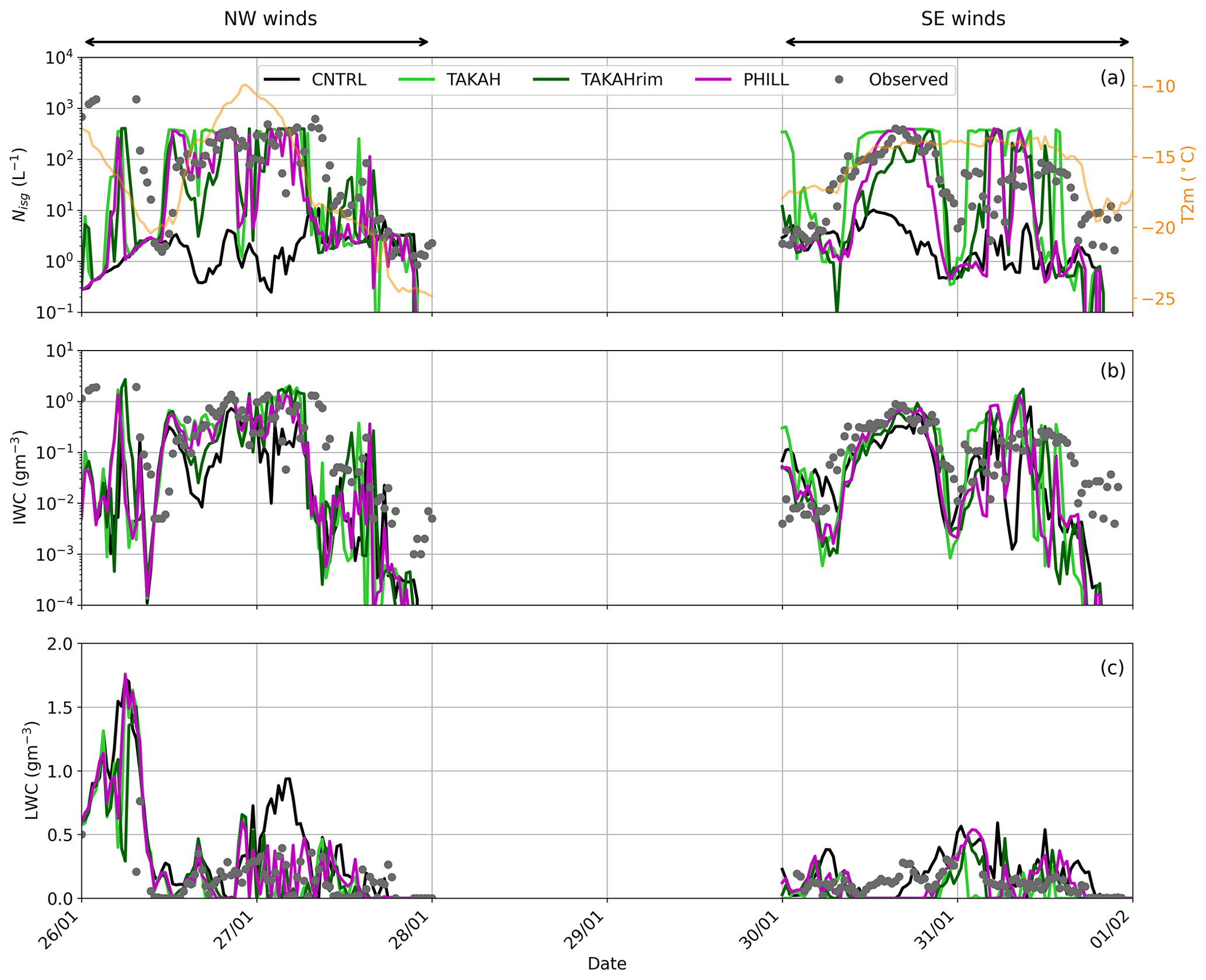
Figure 3 Time series of (a) total N_isg and temperature at 2 m height (orange line), (b) IWC, and (c) LWC, predicted by the CNTRL (black line), TAKAH (light green line), TAKAHrim (dark green), and PHILL (magenta line) simulations between 26 January and 1 February 2014. The gray dots in all three panels represent the 2D-S ICNCs, the inferred IWC, and the CDP LWC measured at the JFJ station, respectively. Note the logarithmic y axes in panels (a) and (b).

During the NW flow, between 26 and 28 January, the measured ICNCs exceed 100 L⁻¹ for > 50 % of the time, whereas during the SE flow, the ICNCs usually fluctuate between 10 and 100 L⁻¹ (Fig. 3a). The highest ICNCs are generally observed at temperatures higher than $\sim -\mathrm{15}$ ^∘C, where SIP processes are thought to be dominant and primary ice nucleation in the absence of bioaerosols is limited (e.g., Hoose and Möhler, 2012; Kanji et al., 2017). The CNTRL simulation fails to reproduce N_isg higher than 10 L⁻¹, with the mean simulated values being ∼ 2–2.5 L⁻¹ during both periods. At the same time, the mean observed ICNC values are ∼ 200 (70) L⁻¹ during the NW (SE) case. Thus, CNTRL systematically underestimates the amount of ice by up to 2 orders of magnitude, which is also consistent with the interquartile statistics presented in Table 3. With the HM process being totally ineffective in the prevailing temperatures, this discrepancy suggests that ice crystals produced by heterogeneous ice nucleation in CNTRL are not high enough to match the observations. A similar discrepancy between predicted INPs and measured ICNCs was also documented in Lloyd et al. (2015).

Table 3 The 25th, 50th (median), and 75th percentiles of ICNC (per liter) time series.

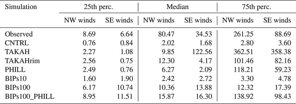
Activating the BR process in TAKAH, TAKAHrim, and PHILL simulations is found to produce N_isg as high as 400 L⁻¹ during both case studies (Fig. 3a), resulting in a substantially better agreement with observations. At times when the simulated temperatures drop below $\sim -\mathrm{18}$ ^∘C, the N_isg modeled by all three simulations coincide with the CNTRL simulation. At relatively warmer subzero temperatures, though, the significant contribution of the BR process is evident, elevating the predicted N_isg by up to 3 orders of magnitude during the NW case and by more than 2 orders of magnitude during the SE case. Although the median N_isg in all three sensitivity simulations with active breakup remains underestimated compared to observations during the NW flow, TAKAH seems to produce unrealistically high median and 75th percentile values during the SE flow (Table 3). Indeed, focusing on the N_isg time series (Fig. 3a), TAKAH is, ∼ 25 % of the time, shown to overestimate the observed ICNCs by a factor of ∼ 3, reaching up to a factor of 10 on 30 January at 00:00 UTC. TAKAHrim and PHILL, on the other hand, produce more reasonable concentrations of ice particles throughout both case studies, with the N_isg values in the 75th percentile exceeding 100 (50) L⁻¹ during the NW (SE) case study (Table 3), which is found to reduce the gap between observations and model predictions.

It is worth noting that, despite the fact that the Takahashi parameterization (Eq. 2) is applied to both TAKAH and TAKAHrim simulations, the former seems to systematically overestimate the number of secondary ice fragments, while the latter produces ICNCs that are more consistent with the observations. Hence, the Takahashi parameterization predicts reasonable results if it is allowed to generate fragments from collisions between rimed ice particles only (Sect. 2.4).

Table 4 The 25th, 50th (median), and 75th percentiles of IWC (in grams per cubic meter; hereafter gm⁻³) time series.

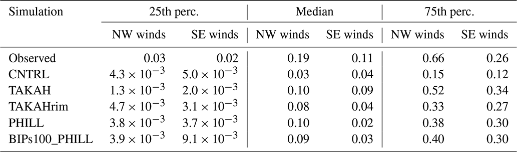
The observed IWC time series (Fig. 3b) are frequently reaching ∼ 1 gm⁻³ during the NW case, with the median values being a factor of 2.5 higher than those observed during the SE case (Table 4). This indicates the presence of more massive ice particles when higher updraft velocities prevail. The CNTRL simulation cannot produce IWC values > 0.8 gm⁻³ and is, most of the time, below the observed range. Adding a description of the BR process (i.e., in TAKAH, TAKAHrim, and PHILL) sufficiently increases the modeled IWC by up to ∼ 1 order of magnitude between 26 January 12:00 UTC and 27 January 06:00 UTC, when the modeled N_isg exceeds 100 L⁻¹, and the temperature remains higher than −16 ^∘C. The same conditions are observed in the SE case, between 12:00 and 18:00 UTC on 30 January, when IWC shows a ∼ 3 fold enhancement reaching the observed levels. The IWC values in the third quartile predicted by TAKAH, TAKAHrim, and PHILL are more than a factor of 2 higher than the ones predicted by CNTRL (Table 4). This increase improves the model performance, although the modeled IWC remains slightly underestimated (overestimated) during the NW (SE) case. The size distribution of the three ice species considered in the M05 scheme (Fig. S4) reveals that the implementation of the BR mechanism leads to elevated concentrations of relatively smaller cloud ice crystals but, at the same time, increases the concentrations of snow particles. This is the reason why the modeled total ice mass is also increased compared with the CNTRL simulation.

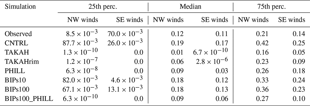
The comparison of the simulated cloud LWC with the concurrent CDP observations at JFJ is presented in Fig. 3c. The LWC values recorded during the NW case are highly variant, reaching up to 0.75 gm⁻³, which is substantially higher than the respective maximum LWC observed during the SE case (0.30 gm⁻³). On 26 January before 12:00 UTC, all sensitivity simulations predict LWC > 1 gm⁻³, which, however, cannot be validated against measurements due to missing data in the CDP time series. Note that this period is excluded from the statistics derived in Table 5. The CNTRL simulation is found to overestimate the cloud LWC, predicting 0.42 (0.25) gm⁻³ in the third quartile, which is a factor of ∼ 2 higher than the observed values during the NW (SE) case (Table 5).

The modeled LWC in the 75th percentile is decreased by a factor of 1.5–5 in the simulations that account for the BR process (Table 5), improving the agreement with observations (Fig. 3c). The reduction in LWC is expected, considering that the higher N_isg produced when BR is activated can readily deplete the surrounding droplets under liquid water subsaturated conditions through the WBF process. This introduces a challenging environment to simulate, as the model is sometimes seen to convert water to ice too rapidly, leading to cloud glaciation (e.g., on 30 January after 12:00 UTC). Despite all sinks of cloud water (i.e., condensation freezing, WBF, or riming), observations at JFJ suggest that mixed-phase regions are generally sustained (Lloyd et al., 2015). This is particularly true for the NW case, when the sufficiently large updrafts caused by the steep ascent of the air masses help maintain the supersaturation with respect to liquid water (Lohmann et al., 2016). PHILL and TAKAHrim can more efficiently sustain the observed mixed-phase conditions compared to TAKAH, which frequently results in explosive ice multiplication – especially during the SE case – leading to an underestimation of the LWC (see Fig. 3c and Table 5). TAKAH is, therefore, excluded from the following discussion, as it fails to reproduce an accurate liquid-ice-phase partitioning.

Table 5 The 25th, 50th (median), and 75th percentiles of LWC (in gm⁻³) time series.

The time-averaged vertical profiles of cloud ice (N_i), graupel (N_g), snow (N_s), and total N_isg number concentrations are illustrated in Fig. 4 for the CNTRL, TAKAHrim, and PHILL simulations. The mean N_i (Fig. 4a) and N_isg profiles (Fig. 4d) are enhanced by up to 2 orders of magnitude in TAKAHrim and PHILL compared to CNTRL. During the NW flow, both simulations, including the BR process, produce a similar vertical distribution of the ice hydrometeors in the lowest 1–1.5 km in the atmosphere. This is not the case for the SE case, where TAKAHrim seems to predict a rapid decrease in N_i and N_s and, thus, in total N_isg with altitude. The main difference between these two simulations lies in the fact that the total LWC and, hence, the probability of riming, decreases with height, limiting the efficiency of BR in TAKAHrim. This become more evident during the SE case, where mixed-phase conditions are exclusively confined below 1.5 km in the atmosphere (Sect. 3.1.1). However, we cannot estimate which vertical distribution better represents reality, due to the lack of corresponding measured profiles. TAKAHrim coincides with PHILL only when there is sufficient liquid water in the atmosphere, allowing for the riming of the ice hydrometeors. Moreover, at heights above ∼ 2.5 km, where the simulated temperatures drop well below −20 ^∘C (Fig. S5), all three simulations are seen to produce similar results. This implies the greater importance of SIP through BR at heights below 2–3 km in the atmosphere (i.e., in the temperature range between ∼ −18 ^∘C and ∼ −10 ^∘C).

Figure 4 Mean vertical profiles of (a) N_i, (b)  N_g, (c) N_s, and (d) total N_isg predicted by the CNTRL (black), TAKAHrim (dark green), and PHILL (magenta) simulations for the NW (solid lines) and SE (dashed lines) cases. Note the different scale on the x axis of the N_g vertical distribution. The height is given in kilometers above ground level (hereafter km a.g.l.).

Graupel number concentrations (Fig. 4b) do not contribute much to the modeled ice phase, especially during the SE case when the simulated N_g is negligible compared with the N_i and N_s (Fig. 4c). In the M05 scheme, a portion of the rimed cloud or rain water onto snow is allowed to convert into graupel (Reisner et al. 1998), provided that snow, cloud liquid, and rain water mixing ratios exceed a threshold of 0.1, 0.5, and 0.1 g kg⁻¹, respectively. These mixing ratio thresholds for graupel formation are arbitrary and might not be suitable for the examined conditions, preventing the formation of graupel from rimed snowflakes (Morrison and Grabowski, 2008). During the NW case, however, we can identify substantially higher N_g than the SE case, owing to the presence of sufficient supercooled liquid water especially during the first half of 26 January. Activating the BR mechanism in TAKAHrim and PHILL generally decreases the simulated N_g in both cases (Fig. 4c), suggesting that the breakup of graupel contributes to ice multiplication.

The mean vertical profile of N_s (Fig. 4c) seems to follow the respective profile of N_i (Fig. 4a). Unlike the graupel concentrations, including the BR mechanism is found to enhance N_s up to 1 order of magnitude compared to the CNTRL simulation. Focusing on a single model time step when the BR mechanism is activated, the size distribution of snow particles shown in the Fig. S4 reveals that the increase in snow number concentrations can reach up to 2 orders of magnitude during the NW case. This is a logical consequence of the increase in the number concentration of ice crystals, which are converting to snow particles after ice crystal growth (i.e., cloud-ice-to-snow autoconversion) when surpassing a characteristic mean diameter of 250 µm. This will be discussed in detail in the following section. Since TAKAHrim and PHILL provide comparable results in terms of the in-cloud phase partitioning, we focus the subsequent discussion on the PHILL simulation because it offers the opportunity to explore the sensitivity of simulation results to parameters not considered by the Takahashi formulation.

3.1.1 Conditions favoring BR in the two considered events

The temporal evolution of the vertical profiles of N_isg, IWC, and LWC can provide valuable insight on the drivers of enhanced ice formation in the wintertime alpine MPCs. The presence of a seeder–feeder cloud system with sustained mixed-phase conditions confined to levels below ∼ 3 km (∼ 1.5 km) in the NW (SE) case and a pure ice cloud aloft is revealed in Fig. 5. Such configurations are a well-known type of orographic multi-layer cloud that enhances precipitation over mountains (e.g., Browning et al., 1974, 1975; Roe, 2005). Cloud condensation is promoted by the synergy between a mid-latitude frontal system and its orographically induced ascent over the mountain range (Fig. 1). The separation between the seeder and feeder clouds is often nonexistent, meaning that ice seeding can occur either in layered clouds or internally within one cloud (Roe, 2005; Proske et al., 2021). In the first case, which seems to occur here as well, there can be a vertical continuum of cloud condensates between the seeder and the feeder cloud due to precipitation of ice crystals from the higher-level cloud (Fig. 5a). This means that the seeding ice crystals fall through subsaturated cloud-free air before reaching the feeder region of the cloud and might sublimate. The remote sensing analysis over Switzerland presented by Proske et al. (2021), showed that in-cloud seeding occurs in 18 % of the observations, while the external seeder–feeder mechanism is present 15 % of the time when the seeder is a cirrus cloud.

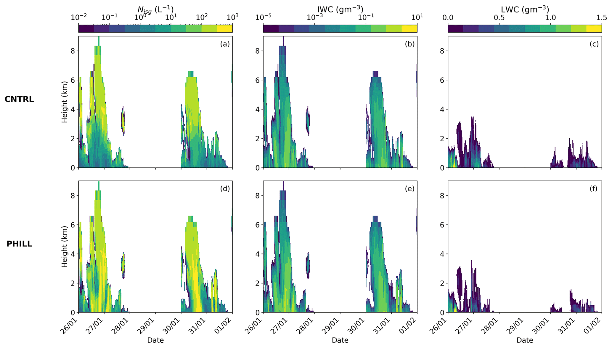
Figure 5 Time–height plots of total N_isg (a, d), IWC (b, e), and LWC (c, f) produced by CNTRL (a–c) and PHILL (d–f) simulations between 26 January and 1 February 2014. The height is given in km a.g.l.

To illustrate the processes taking place during the two cases of interest, Fig. 6 displays the tendency of primary and secondary ice production, as well as the growth of ice particles through deposition, riming, and aggregation from the CNTRL and PHILL simulations at 17:00 (19:00) UTC on 26 (30) January. The vertical profiles on 26 January are taken within the seeder–feeder event, while those on 30 January are taken when the high-level cloud associated with the warm front has already passed the region of interest. Upon arrival of the frontal system on 26 January, CNTRL indicates a rapid increase in the total N_isg near the cloud top (Fig. 5a), which is not shown in the vertical profile of primary ice production rates taken at 17:00 UTC (Fig. 6a). The ice particles consisting the seeder cloud are, therefore, formed far from the JFJ station and seem to be advected over the domain of interest. Primary ice crystals are formed in both cases below 2 km in the feeder cloud at temperatures lower than −30 ^∘C through heterogeneous freezing (Fig. 6a). At these heights, supercooled liquid water is also present (Fig. 5c), and the newly formed ice particles start growing initially by vapor deposition due to supersaturation with respect to ice, followed by riming (Fig. 6b). This is also indicated by the increased IWC values closer to the ground (Fig. 5b).

Figure 6 Vertical profiles of (a, d) primary and secondary ice production, (b, e) riming and vapor deposition or sublimation, and (c, f) snow aggregation produced by the CNTRL (a–c) and PHILL (d–f) simulations at 17:00 UTC on 26 January (solid line) and at 19:00 UTC on 30 January (dashed line). The vertical profile of simulated temperature is also superimposed in panel (a). The cloud liquid water content (Q_c) is shown in panels (b) and (e) to represent the tendency due to riming, while the mass mixing ratio of the ice and snow species (Q_i+Q_s), represents the relative tendencies due to vapor deposition or sublimation. Note that the tendencies due to snow aggregation in panels (c) and (f) are presented in absolute values. The height is given in km a.g.l.

Focusing on the ice-seeding event of 26 January, the enhanced aggregation rate observed at heights above ∼ 2.5 km in the atmosphere indicates the enhanced collision efficiencies of precipitating ice particles while falling from the seeder cloud (Fig. 6c). Note that a portion of the sedimented ice particles sublimates before reaching the feeder cloud at heights ∼ 3–5 km, indicating the prevailing unsaturated conditions in this layer (Fig. 6b). Within this layer, the aggregation of snowflakes weakens, while it is enhanced again when the falling hydrometeors enter the feeder cloud. The bottom line is that, even under the simulated seeder–feeder events, the concentrations of ice particles reaching the ground in CNTRL remain severely underestimated (Sect. 3.1). Despite the low concentrations of ice crystals simulated by the CNTRL simulation, the low-level cloud is glaciated more frequently during the SE than during the NW winds case (Fig. 5c). This is probably because of the higher updraft velocities prevailing until 28 January (Fig. 2d), preventing ice crystals from falling through the lower parts of the cloud (Lohmann et al., 2016).

Activating the BR mechanism along with the seeding of precipitating hydrometeors in PHILL shifts the simulated N_isg towards higher concentrations that are found to exceed 300 L⁻¹ in the lower-level part of the cloud (Fig. 5d). On 26 January, the mode of the cloud ice distribution shifts to slightly bigger sizes, while on 30 January the modal sizes become almost an order of magnitude smaller compared with the CNTRL simulation (Fig. S4). The enhanced concentrations of bigger ice particles simulated in the first case experience rapid growth through vapor deposition and riming (Fig. 6e), causing a slight increase in the simulated IWC (Fig. 5e) at the expense of the surrounding cloud droplets in the low-level feeder cloud (Fig. 5f). Nevertheless, the smaller ice particles simulated in the second case grow less efficiently through vapor deposition, while the explosive multiplication of ice through BR seems to fully glaciate the low-level cloud below ∼ 1 km, resulting in an almost zero riming rate (Fig. 6e). The reduced primary ice production rate observed during both case studies is a consequence of the depletion of liquid water when BR is considered (Fig. 6d). A suppression of heterogeneous ice nucleation following the introduction of SIP into models has already been reported in previous studies (Phillips et al., 2017b; Dedekind et al., 2021; Zhao and Liu, 2021b).

The key difference between CNTRL and PHILL simulations is that the latter takes advantage of the enhanced ice particle growth through aggregation, while falling to the feeder cloud below ∼ 2 km where large snowflakes coexist with smaller ice crystals (Figs. 4a, 6a, 6d). This allows for differential settling, which enhances collision efficiency facilitating ice multiplication through BR. This is the reason why the vertical profile of secondary ice formation agrees with the corresponding profile of aggregation during both case studies (Fig. 6d, f). On 26 January, the first secondary ice particles start forming already within the seeder cloud, with the contribution of SIP increasing considerably when reaching the feeder cloud, where the tendency, due to SIP, is more than 3 orders of magnitude higher than primary ice production (Fig. 6d). The significant role of SIP stands out also on 30 January at altitudes below 2 km. It is, therefore, essential to consider SIP though BR in the feeder cloud, in order to achieve the enhanced levels of ICNCs frequently observed within seeder–feeder events in the alpine region. This is in agreement with the observational study of Ramelli et al. (2021) on an ice-seeding case occurring in the region around Davos in the Swiss Alps. In this study, they proposed that SIP though HM and BR were necessary to explain the elevated ICNCs in feeder clouds.

A classification of the dominant type of precipitation was applied to the polarimetric data collected by a weather radar deployed at the Kleine Scheidegg station (2061 m a.s.l) during the SE case between 30 and 31 January (Fig. S6). In the derived time series, we can identify periods when individual ice crystals (not aggregated and not significantly rimed) dominate over the entire precipitation column, followed by periods when a clear stratification is present with ice crystals aloft and mostly aggregates and rimed ice particles below. This stratification is observed on 30 January at 19:00 UTC when the model tendencies are extracted (dashed lines in Fig. 6). Allowing for the BR process in PHILL results in an enhancement of 2 orders of magnitude in the aggregation rates close to the ground, which can better reproduce the signatures observed in the hydrometeor classification at that time. An increase in the simulated aggregates and rimed particles is expected to increase orographic precipitation, which is important given that these low-level feeder clouds are incapable of producing significant amounts of precipitation. Indeed, the mean surface precipitation produced by PHILL is increased by 30 % (10 %) during the NW (SE) case compared with CNTRL (Fig. S7), which is in contrast to Dedekind et al. (2021), where the activation of the BR process is found to suppress the regions of strong surface precipitation. This was attributed to the limited efficiency of the small secondary ice particles to grow sufficiently to precipitation sizes when the local updrafts lift them to the upper parts of the cloud that were glaciated. The radar-based hydrometeor classification reveals also the predominance of ice crystals at the beginning and the end of the precipitating periods (e.g., on 30 January at 15:00–17:30 UTC or 31 January at 04:30–06:00 UTC), which is again more consistent with the vertical profile of N_i produced by PHILL rather than the CNTRL simulation (Fig. S6, S8).

3.2 Sensitivity to the injection of ice crystals from the surface

In this section, we examine if the surface-originating small ice particles could have the potential to initiate and enhance ice particle growth in the near-surface MPCs present in our case studies. Figure 7 illustrates two additional WRF simulations – BIPs10 and BIPs100 – where the ice crystal source applied to the first model level is equal to 10 and 100 L⁻¹, respectively (Table 2). Note that these two sensitivity tests do not consider any SIP process to analyze the influence of BIPs only. The total N_isg values produced in BIPs10 are only slightly increased compared to the CNTRL simulation and generally remain outside the observed range at JFJ (Fig. 7a). An order of magnitude increase in the applied NBIPs is seen to enhance the modeled N_isg during both case studies; however, our simulations are still lacking ice particles. This is particularly evident during the NW winds case, where the simulated N_isg varies most of the time around 10 L⁻¹, remaining an order of magnitude lower than the observations. During the SE case, the model performance is slightly improved, with the N_isg reaching up to ∼ 25 L⁻¹ in BIPs100, which occasionally falls within the lower limit of the observed ICNC values (e.g., in the evening of 31 January). At times when the detected ICNCs remain quite low (i.e., of the order of 10 L⁻¹), the contribution of blowing snow particles probably from the Aletsch Glacier is sufficient to explain the observations at JFJ.

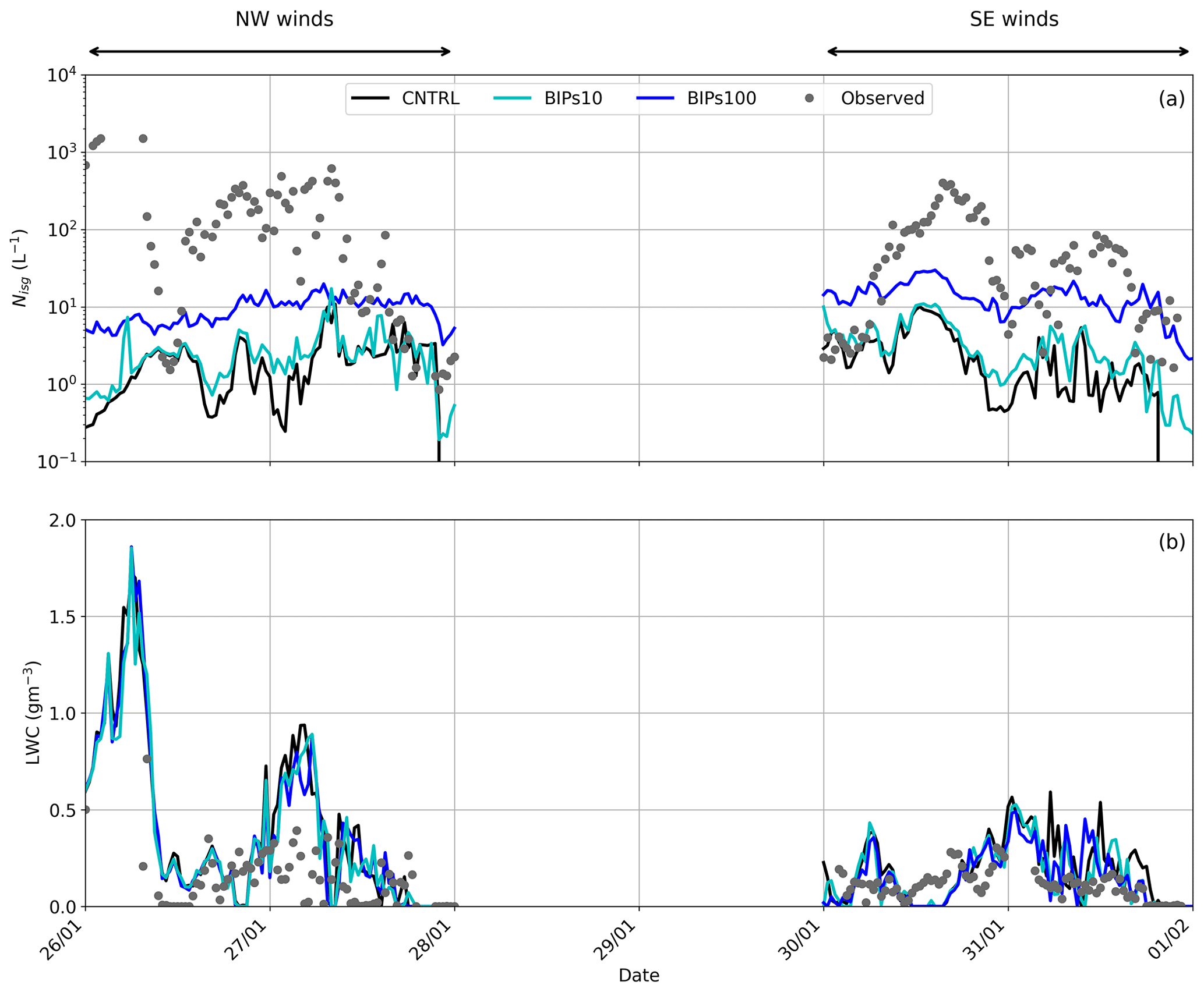
Figure 7 Time series of (a) total N_isg and (b) LWC predicted between 26 January and 1 February 2014 by the two sensitivity simulations accounting for the effect of blowing snow, i.e., BIPs10 (cyan line) and BIPs100 (blue line).

As indicated in Fig. 7b, during the NW flow the simulated LWC at the first model level in BIPs10 and BIPs100 almost coincides with the CNTRL simulation of WRF. The three sensitivity simulations are producing comparable median and quartile LWC values (Table 5), with BIPs10 and BIPs100 producing median LWC values closer to the observed ones during the SE flow. When comparing against the LWC values in the third quartile though, the two simulations lead to an overestimation up to a factor of ∼ 1.5 during both case studies. Given that there is approximately a factor of > 20 (5) difference between the modeled and observed ICNCs during the NW (SE) winds case (Table 3), overall Fig. 7 reveals that the addition of a source of ice crystals from the effect of blowing snow cannot account for the observed liquid-ice-phase partitioning in the simulated orographic MPCs.

Our findings are in contrast with the modeling study of Farrington et al. (2016), where a different approach was proposed to include the surface effect on the ICNCs simulated with WRF. In this study, a single model domain was used with a horizontal resolution of 1 km. To account for the flux of hoar crystals being detached from the surface by mechanical fracturing, Farrington et al. (2016) included a wind-dependent surface flux of frost flowers adapted from Xu et al. (2013). Despite the improved performance of WRF in terms of predicted ICNCs and LWC, the wind-dependent formulation of the surface flux caused the modeled ICNCs to become strongly correlated with the simulated horizontal wind speed – a behavior that was not confirmed by the observations of Lloyd et al. (2015). Nonetheless, the highest observed ICNCs at the beginning of the NW case correspond to the time when both the observed and modeled wind speed is the strongest (Fig. 2c), implying that a wind-dependent surface flux of BIPs could potentially elevate the simulated N_isg to the observed levels at this time.

3.3 The synergistic impact of BR and surface-induced ice crystals

It is deducible from the above discussion that the sole inclusion of a constant source of BIPs in our simulations cannot efficiently bridge the gap between modeled and measured ICNCs. Our aim in this section is to explore the combined effect of SIP through BR and blowing snow on the simulated orographic MPCs, since both processes are deemed to be important when trying to explain the high ICNCs observed in alpine environments. This is addressed in the final sensitivity simulation, BIPs100_PHILL, the results of which are compared with the CNTRL and PHILL simulations in Fig. 8.

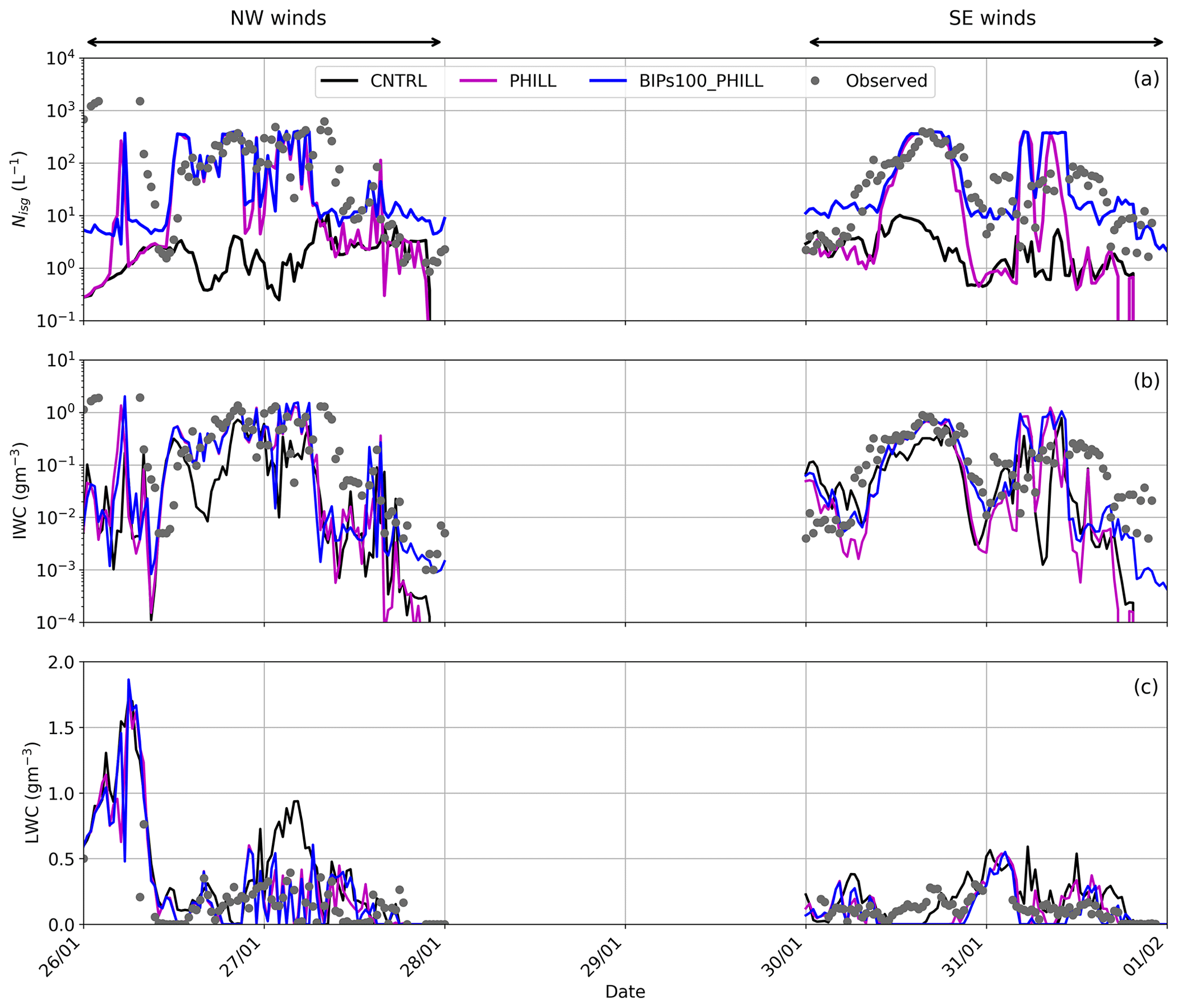
Figure 8 Time series of (a) total N_isg, (b) IWC, and (c) LWC predicted between 26 January and 1 February 2014 by the sensitivity simulation BIPs100_PHILL (blue line), which examines the combined effect of ice multiplication through BR and blowing snow.

In terms of the modeled ice particle concentrations, the combination of the simplified blowing snow treatment and BR parameterization can account for most of the discrepancy between modeled and observed ICNCs, particularly during the SE case (Fig. 8a), when the simulation leads to a best agreement with the observed interquartile values (Table 3). BIPs100_PHILL and CNTRL generally differ by an average factor of ∼ 100 (40) during the NW (SE) case, with the former producing N_isg values that are sometimes elevated by up to ∼ 3 (2) orders of magnitude (Fig. 8a). Compared to the PHILL setup, including a source of BIPs is found to improve the modeled ICNCs close to the surface episodically – for instance, in the evenings of 30 and 31 January, with the N_isg in BIPs100_PHILL efficiently reaching the observed levels (Fig. 8a). Note that BIPs can contribute to the modeled N_isg even without the presence of a near-surface orographic cloud (e.g., Geerts et al., 2015; Beck et al., 2018). For instance, BIPs100_PHILL is the only sensitivity simulation producing high N_isg values in the evenings of 27 and 31 January when the low-level cloud is dissipated (Fig. 5c, f). In the former case, however, the model results in an overestimate of the ICNCs, which is also observed during the early hours of 30 January, suggesting that the applied source of ice crystals is unrealistically high at this time.

As the mixed-phase conditions are sustained throughout both case studies (Fig. 8c), the plume of ice crystals is mixed into an ice-supersaturated environment and, thus, BIPs are expected to promote ice growth through their interaction with the surrounding supercooled liquid droplets and (ice) supersaturated air. The number of BIPs reaching the cloud base might not be large, but their presence is expected to further facilitate the action of the BR mechanism, considering the depositional growth they will undergo within the supercooled boundary layer cloud. This is illustrated, for example, with the concurrent increase in N_isg and IWC observed on 30 January at approximately 21:00 UTC (Fig. 8a, b) in the presence of the low-level cloud (Fig. 8c). Note that the elevated N_isg caused by the addition of BIPs is not always followed by an efficient increase in the simulated IWC. This can be observed, for instance, on 27 January at 12:00 UTC or in the evening of 31 January (Fig. 8b).

A discrepancy between modeled and observed IWC was also highlighted in the study of Farrington et al. (2016) and was attributed to the small sizes of the hoar frost particles assumed (i.e., 10 µm). Although here BIPs are assumed to have sizes of 100 µm, the underestimation in the cloud IWC has still not been overcome. This suggests that the applied source of BIPs combined with the effect of SIP through BR shifts the ice particle spectra to smaller sizes, which are not very efficient at riming and the WBF process and, thus, do not always contribute to significant increases in IWC values. Overall, the interquartile values presented in Table 4 reveal that BIPs100_PHILL and PHILL yield almost identical IWC values, suggesting that the implementation of a constant source of BIPs does not further improve the representation of the total ice mass, despite the improvements in the simulated N_isg. Focusing on the LWC values in the third quartile, though, including a source of BIPs results in better agreement with the CLACE observations during the SE case, while it is shown to have little effect on the cloud liquid phase during the NW case (Table 5). Despite the increase in the modeled N_isg observed in BIPs100_PHILL, especially during the SE case, the liquid water in the low-level orographic cloud is not further depleted (Fig. 8c). This is presumably because the mean surface precipitation produced is also enhanced by almost ∼ 20 % compared to PHILL (Fig. S7), which seems to balance the excessive ice production.

One final point that is worth noting here is that there are still certain periods when BIPs100_PHILL fails to reproduce the observed range of ICNCs. This could imply the potential contribution of additional ice multiplication processes to the observed ice particle concentrations. Indeed, the seeder–feeder configuration observed in the examined case studies could favor the fragmentation of sublimating hydrometeors while falling through an subsaturated environment before entering the feeder cloud (e.g., Bacon et al., 1998; Deshmukh et al., 2022). The so-called sublimational breakup is an overlooked SIP process which is not yet described in the M05 scheme. Also, note that the periods when the modeled ICNCs remain below the observed ice number levels are mainly identified when the simulated temperature drops below −15 ^∘C and the wind speed exceeds 10 ms⁻¹ or even 20 ms⁻¹ (e.g., in the morning of 26 or 27 January at around 12:00 UTC). This is when the incorporation of surface-based processes becomes of primary importance. The simplified methodology we followed here, although instructive, faces several limitations. For instance, the constant source of BIPs is sometimes found to overestimate the modeled N_isg and IWC. In order to accurately assess the potential role of the snow-covered surfaces in elevating the simulated ICNCs, an improved spatiotemporal description of the concentration and distribution of BIPs is required. Furthermore, the applied ice crystal source is independent of some key parameters controlling its resuspension, such as the horizontal wind speed, the updrafts, or the friction velocity (e.g., Vionnet et al., 2013, 2014). For example, in the early morning hours of 26 January, the high simulated horizontal and vertical velocities (Fig. 2c, d) are expected to loft significant NBIPs into the cloud layer, owing to enhanced mechanical mixing and momentum flux close to the surface. Nonetheless, the contribution of the induced plume of BIPs remains constant throughout the NW case study (Fig. 7a), which seems to lead to an underestimation of the total ice particle concentration and mass. A more realistic parameterization of the BIPs flux or the coupling with a detailed snowpack model (e.g., Sharma et al., 2021) would, therefore, be essential for a more accurate representation of the effect of blowing snow.

4 Summary and conclusions

This study employs the mesoscale model WRF to explore the potential impact of ice multiplication processes on the liquid-ice-phase partitioning in the orographic MPCs observed during the CLACE 2014 campaign at the mountain-top site of JFJ in the Swiss Alps. The orography surrounding JFJ channels the direction of the horizontal wind speed, giving us the opportunity to analyze two frontal cases occurring under NW and SE conditions.

DS and BR mechanisms were implemented in the default M05 scheme in WRF, in addition to the HM parameterization, which, however, remained inactive in the simulated temperature range (−10 to −24 ^∘C). The DS process is parameterized following either the latest theoretical formulation developed by Phillips et al. (2018) or the more simplified parameterization proposed by Sullivan et al. (2018a). Our sensitivity simulations revealed that the DS mechanism is ineffective in the two considered alpine MPCs, even under the higher updraft velocity conditions associated with the NW winds case study, owing to the lack of large drops required for the process.

To parameterize the number of fragments generated per ice–ice collision, we followed again two different approaches. We used either the simplified temperature-dependent formulation of Takahashi et al. (1995) scaled for the size of the particle that undergo fragmentation (Sotiropoulou et al., 2021a) or the more advanced physically based Phillips et al. (2017a) parameterization. It is important to apply the Takahashi parameterization only to consider collisions between rimed ice particles, otherwise the number of generated fragments is significantly overestimated. Including a description of the BR mechanism is essential for reproducing the ICNCs observed in the simulated orographic clouds, especially at temperatures higher than ∼ −15 ^∘C, where INPs are generally sparse. SIP through BR is found to enhance the modeled ICNCs by up to 3 (2) orders of magnitude during the NW (SE) case, improving the model agreement with observations. This ice enhancement can cause up to an order of magnitude increase in the mean simulated IWC values compared with the CNTRL simulation, which is attributed to the enhanced ice crystal growth and cloud-ice-to-snow autoconversion. The increase in the simulated ICNCs also depletes the cloud LWC by at least a factor of 2 during both cases, which is more consistent with the measured LWC values.

One of the most interesting outcomes of this study is the association of the enhanced BR efficiency with the occurrence of in-cloud seeder–feeder events, which are commonly found in Switzerland (Proske et al., 2021). While ice-seeding situations are associated with enhanced orographic precipitation in the alpine region, the CNTRL simulation fails to reproduce the elevated ICNCs reaching the ground. The falling ice hydrometeors experience efficient growth through aggregation in the seeder part of the cloud, which is enhanced when reaching the feeder cloud at altitudes below 2 km, where primary ice crystals form and grow through vapor deposition and riming. Aggregation of snowflakes seems to be the major driver of secondary ice formation in the examined seeder–feeder events. SIP through BR is initiated already within the seeder cloud, while it becomes immensely important in the feeder cloud, where its production rate exceeds the one of primary ice formation. The increased generation of secondary ice fragments does not always lead to ice explosion and cloud glaciation, as it is followed by an enhancement in the precipitation sink owing to a shift in the ice particle spectrum. Including a description of the BR mechanism is, therefore, crucial for explaining the ice particle concentration and mass observed in the low-level feeder clouds.

To assess the potential role of blowing snow in the simulated orographic clouds, a constant source of ice crystals was introduced in the first atmospheric level of WRF. Our results indicate that blowing snow alone cannot explain the high ICNCs observed at JFJ, but when this source is combined with the BR mechanism then the gap between modeled and measured ICNCs is sufficiently bridged. The biggest influence of blowing snow is mainly detected at times when the simulated temperatures are low enough (<−15 ^∘C), while the presence of a low-level cloud is required for SIP to manifest. The concentrations of BIPs reaching the cloud base are not high, but when they are mixed among supercooled liquid droplets then they are expected to grow, facilitating ice multiplication through BR. Nonetheless, including a wind dependence or a spatiotemporal variability in the applied ice crystal source would be essential to provide a more precise description of the effect of blowing snow on the simulated clouds.

Overall, our findings indicate that, outside the HM temperature range, a correct representation of both secondary ice (through BR) and an external ice-seeding mechanism, which is primarily precipitating ice particles formed aloft and, to a lesser degree, windblown ice from the surface, is fundamentally important for accurately predicting the liquid-ice-phase partitioning and properties of MPCs. Given the high frequency of seeder–feeder events in orographic environments, including the new physics of BR may address a large source of predictive bias in atmospheric models.