the Creative Commons Attribution 4.0 License.
the Creative Commons Attribution 4.0 License.
 | 22 Dec 2022
Decoupling impacts of weather conditions on interannual variations in concentrations of criteria air pollutants in South China – constraining analysis uncertainties by using multiple analysis tools
Yu Lin
Qinchu Fan
He Meng
Huiwang Gao
Xiaohong Yao
In this study, three methods, i.e., the random forest (RF) algorithm, boosted regression trees (BRTs) and the improved complete ensemble empirical-mode decomposition with adaptive noise (ICEEMDAN), were adopted for investigating emission-driven interannual variations in concentrations of air pollutants including PM2.5, PM10, O3, NO2, CO, SO2 and NO2 + O3 monitored in six cities in South China from May 2014 to April 2021. The first two methods were used to calculate the deweathered hourly concentrations, and the third one was used to calculate decomposed hourly residuals. To constrain the uncertainties in the calculated deweathered or decomposed hourly values, a self-developed method was applied to calculate the range of the deweathered percentage changes (DePCs) of air pollutant concentrations on an annual scale (each year covers May to the next April). These four methods were combined together to generate emission-driven trends and percentage changes (PCs) during the 7-year period. Consistent trends between the RF-deweathered and BRT-deweathered concentrations and the ICEEMDAN-decomposed residuals of an air pollutant in a city were obtained in approximately 70 % of a total of 42 cases (for seven pollutants in six cities), but consistent PCs calculated from the three methods, defined as the standard deviation being smaller than 10 % of the corresponding mean absolute value, were obtained in only approximately 30 % of all the cases. The remaining cases with inconsistent trends and/or PCs indicated large uncertainties produced by one or more of the three methods. The calculated PCs from the deweathered concentrations and decomposed residuals were thus combined with the corresponding range of DePCs calculated from the self-developed method to gain the robust range of DePCs where applicable. Based on the robust range of DePCs, we identified significant decreasing trends in PM2.5 concentration from 2014 to 2020 in Guangzhou and Shenzhen, which were mainly caused by the reduced air pollutant emissions and to a much lesser extent by weather perturbations. A decreasing or probably decreasing emission-driven trend was identified in Haikou and Sanya with inconsistent PCs, and a stable or no trend was identified in Zhanjiang with positive PCs. For O3, a significant increasing trend from 2014 to 2020 was identified in Zhanjiang, Shenzhen, Guangzhou and Haikou. An increasing trend in NO2 + O3 was also identified in Zhanjiang and Guangzhou and an increasing or probably increasing trend in Haikou, suggesting the contributions from enhanced formation of O3. The calculated PCs from using different methods implied that the emission changes in O3 precursors and the associated atmospheric chemistry likely played a dominant role than did the perturbations from varying weather conditions. Results from this study also demonstrated the necessity of combining multiple decoupling methods in generating emission-driven trends in atmospheric pollutants.
- Article
(2815 KB) - Full-text XML
-
Supplement
(2699 KB) - BibTeX
- EndNote


With rapid economic growth in the past several decades across China, air pollution has become increasingly severe in most parts of the country (Chan and Yao, 2008; He et al., 2002). A turning point emerged in the most recent decade, benefitting from stringent emission control measures implemented in China since 2013, such as the Atmospheric Pollution Prevention and Control Action Plan (APPCAP) (Chen et al., 2020; Vu et al., 2019; Zhang et al., 2020). Trends in long-term monitored pollutants are important indicators of the effectiveness of the emission control policies (Hogrefe et al., 2000; Rao et al., 1997). This is particularly true in China, where air pollutant emissions have not been updated in the annual reports of ecology and environment issued by local governments at the city level since 2014. The Multi-resolution Emission Inventory for China (MEIC) was developed in 2012 by Tsinghua University to estimate anthropological air pollutant emissions, but it was updated every 2–3 years and only up to 2017.
To evaluate existing national emission control strategies in China (such as APPCAP), several studies have analyzed air pollutant concentrations measured at the national monitoring stations (Hu et al., 2021; Xu and Zhang, 2020; Zhao et al., 2021). However, trends and interannual variations in air concentrations of the monitored pollutants were affected by not only emission changes, but also by varying meteorological conditions and/or weather systems (Dang et al., 2021; Lin et al., 2021; Vu et al., 2019; G. Zhang et al., 2019; X. Y. Zhang et al., 2019; Zhao et al., 2020; Henneman et al., 2015; Foley et al., 2015; Astitha et al., 2017; Hogrefe et al., 2002). For example, Zhao et al. (2020) reported that the observed large declines in PM2.5, SO2 and CO concentrations on the national scale during the COVID-19 outbreak were primarily caused by poor dispersion meteorological conditions. Vu et al. (2019) argued that the PM2.5 target of 60 µg m−3 would not have been achieved in Beijing in the winter of 2017 without the favourable weather conditions for rapid dispersion and precipitation scavenging of air pollutants. Similarly, Lin et al. (2021) suggested that meteorological factors significantly reduced O3 concentrations from 2013 to 2020 in eastern and central China, as indicated by the reversed O3 trends after removing the major meteorological effects. It is thus essential to decouple the total trends in pollutant concentrations into portions caused by varying meteorological factors and weather conditions and by emission changes so that the mitigation effects can be evaluated accurately.
In the literature, the multiple linear regression (MLR) method is considered the simplest approach to decouple the effects of meteorological factors from changed emissions on the trends in air pollutant concentrations (Borlaza et al., 2022; Chen et al., 2020; K. Li et al., 2019; Otero et al., 2018; Zhai et al., 2019). However, the MLR analysis sometimes suffers from the auto-correlation inherently existing between different meteorological parameters (Yao et al., 2009). To overcome this weakness, “meteorological normalization” tools have been developed based on statistical modelling (Chen et al., 2020; Gong et al., 2021; Grange and Carslaw, 2019; Li et al., 2020; Xiao et al., 2021; Xue et al., 2020; Zhai et al., 2019). For example, the machine learning techniques, such as the random forest (RF) algorithm and boosted regression trees (BRTs), performed better than the traditional methods like MLR (Carslaw and Taylor, 2009; Grange et al., 2018) or other air quality numerical models like the Weather Research and Forecasting-Community Multi-scale Air Quality model (Vu et al., 2019; Foley et al., 2015; Astitha et al., 2017) in analyzing air quality trends and meteorological impacts. These methods have been used widely in relevant studies across China, e.g., in Beijing (Vu et al., 2019), the Beijing–Tianjin–Hebei region (Qu et al., 2020) and the North China Plain (Y. X. He et al., 2021). In the methods mentioned above, meteorological data are a necessity. In contrast, another exiting method called empirical-mode decomposition (EMD) and its updated version the improved complete ensemble empirical-mode decomposition with adaptive noise (ICEEMDAN) directly decompose time series of air pollutant concentrations and deduct the perturbation from meteorological factors in the residuals (trend) to some extent (Colominas et al., 2014; Fu et al., 2020). It should be pointed out that, due to the non-linearity of chemical reactions related to air pollutants, none of the existing methods is perfect in decoupling the effects of dominant factors on the total trends of pollutant concentrations. To evaluate the uncertainties in trend analysis, combining results from several different methods is recommended (Hogrefe et al., 2002; Qiu et al., 2022; Xiao et al., 2021; Xue et al., 2020).
The updated global air quality guidelines from the World Health Organization (WHO) declared in 2021 brought new challenges to policy makers in establishing more stringent emission control policies, even in the relatively clean regions like South China. For example, air quality in Hainan Province needs to be further improved to meet the new WHO standards, and the demonstration of the Hainan Free Trade Port and the declaration of the province as a National Ecological Civilization Demonstration Zone in China make this task more challenging. Even more challenges exist for the cities in Guangdong Province because of their higher air pollutant concentrations than in Hainan (Gong et al., 2021; He et al., 2017; R. Li et al., 2019; X. Y. Zhang et al., 2019). To accommodate these challenges, the effect of APPCAP needs to be first assessed regionally in South China. For this purpose, we analyzed 7-year (from May 2014 to April 2021) concentration data of six criteria air pollutants (PM2.5, PM10, O3, NO2, CO and SO2) as well as the sum of NO2 and O3 in six cities in South China, of which two (Haikou and Sanya) are in Hainan Province and four (Guangzhou, Shenzhen, Zhuhai and Zhanjiang) are in Guangdong Province. Three different analysis methods were used to identify emission-driven interannual variations and perturbations from varying weather conditions. In addition, a self-developed method was further introduced to constrain analysis uncertainties.
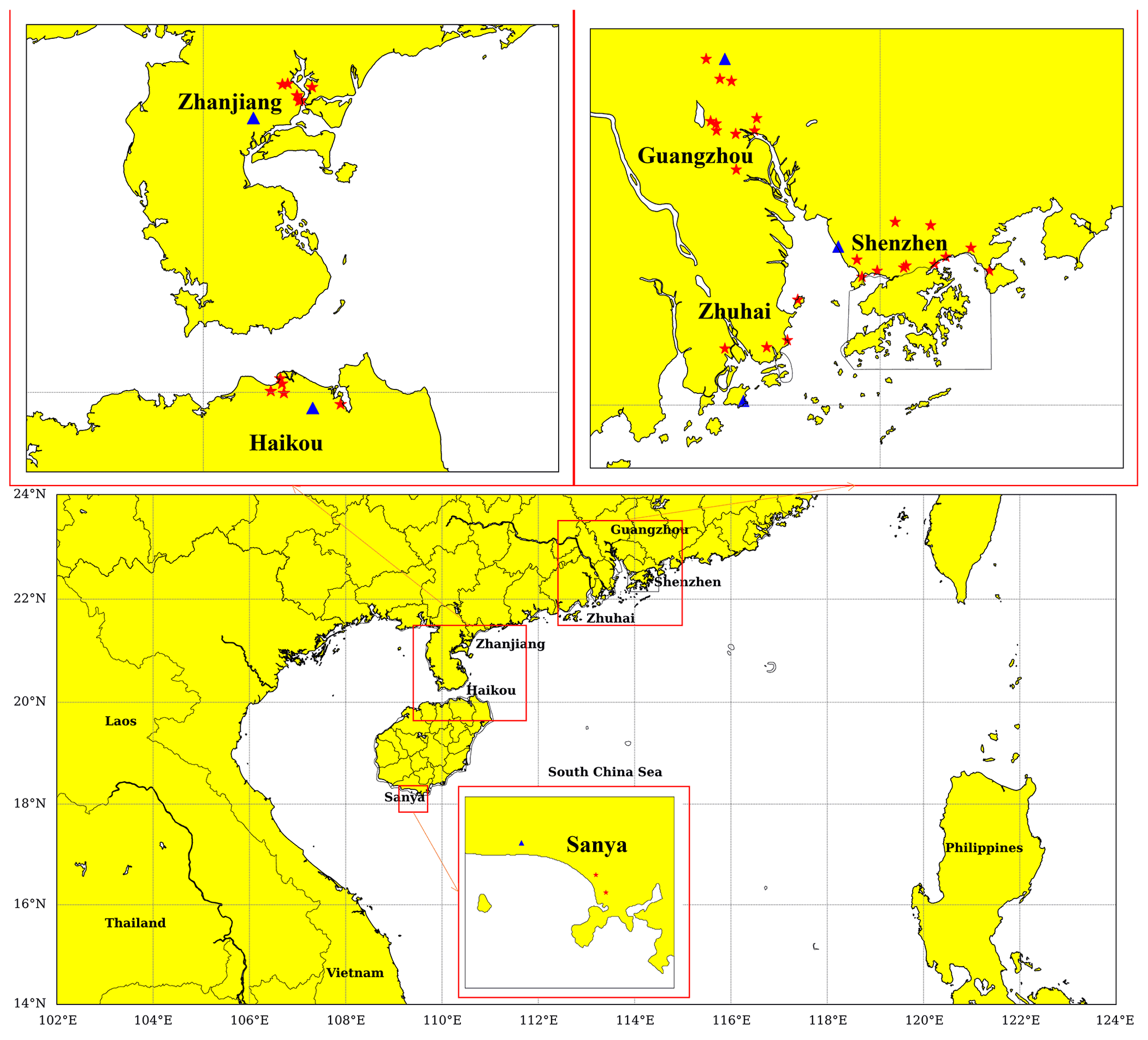
Figure 1Maps of the study areas and locations of air quality monitoring stations (red star) and one meteorological station (blue triangle) in each city.
2.1 Monitoring stations and monitored air pollutant concentrations and meteorological data
Six cities in South China, including Haikou and Sanya in Hainan Province and Guangzhou, Shenzhen, Zhuhai and Zhanjiang in Guangdong Province, were selected in the present study (Fig. 1). There are 2 monitoring stations in Sanya, 4 in Zhuhai, 5 in Haikou, 6 in Zhanjiang and 11 in both Guangzhou and Shenzhen (Fig. 1 and Table S1 in the Supplement). The hourly average air quality data for six criteria pollutants (PM2.5, PM10, O3, NO2, CO and SO2) were downloaded from the China National Environmental Monitoring Centre (CNEMC, http://www.cnemc.cn/sssj/, last access: 13 December 2022) for every monitoring station. The city-specific hourly air quality data represent the average of all the stations in the same city. Data before May 2014 were incomplete, and thus only the data after May 2014 were used for the analysis. One whole-year datum covered May to the next April; e.g., the first-year annual average (referred to as the 2014 annual average in the discussion below) covered May 2014 to April 2015, and the last-year average (referred to as the annual average in 2020 below) covered May 2020 to April 2021. For a pollutant in a city, 52204–58695 hourly data were available in 7 years (Table S2). Note that all concentrations were converted to the values under the standard conditions (273.15 K, 1 atm) for consistency. The sum of NO2 and O3 was also analyzed together with the six pollutants mentioned above, and their sum was calculated by considering their different molecular weights, i.e., [NO2 + O3] = [NO2] × 48 46 + [O3]. Note that concentrations of volatile organic carbons (VOCs) were not reported by CNEMC, and this group of pollutants is not considered in the present study. Thus, a total of 42 cases (seven pollutants in six cities) were analyzed for deweathered trends.
Hourly meteorological data including wind speed (ws), wind direction (wd), air temperature (at), relative humidity (rh) and dew point (dp) were obtained from the meteorological observational station at a nearby airport (Fig. 1 and Table S1), which are accessible from the NOAA Integrated Surface Database (ISD) by using the “worldmet” R package (Carslaw, 2021). To improve the performance of machine learning models (Hou et al., 2022; Shi et al., 2021), other meteorological parameters, including boundary layer height (blh), total cloud cover (tcc), surface net solar radiation (ssr), surface pressure (sp), and total precipitation (tp), which were extracted from the European Centre for Medium-Range Weather Forecasts' Reanalysis-5 (ERA5) hourly data (https://cds.climate.copernicus.eu/, last access: 13 December 2022), and air mass clusters based on the Hybrid Single-Particle Lagrangian Integrated Trajectory (HYSPLIT) 72 h back trajectories at hourly resolution (https://www.ready.noaa.gov/HYSPLIT_traj.php, last access: 13 December 2022) were also used, including for modelling. The meteorological data of each city, ERA5 hourly data and the calculated back trajectories were combined with city-specific hourly air quality data as input for the machine learning analysis.
2.2 Data analysis methods
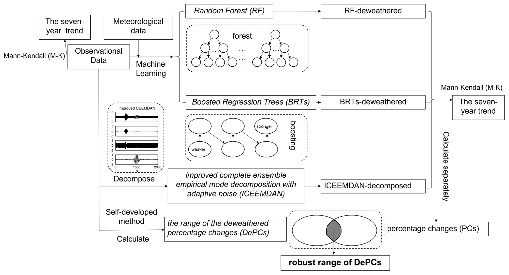
Two machine learning methods, including the RF algorithm and the BRTs, were separately used to calculate the deweathered hourly concentrations. The third method, the ICEEMDAN, was used to decompose hourly residuals of air pollutants. The Mann–Kendall (M–K) method was then applied to the deweathered and decomposed values to extract the trends and calculate the percentage changes (PCs). A self-developed method was further applied to calculate the range of the deweathered percentage changes (DePCs) of air pollutant concentrations on annual scales. The three PCs and DePCs were combined to constrain the uncertainties and generate a robust range of DePCs. Figure 2 shows the framework of this study with the four methods to be applied.
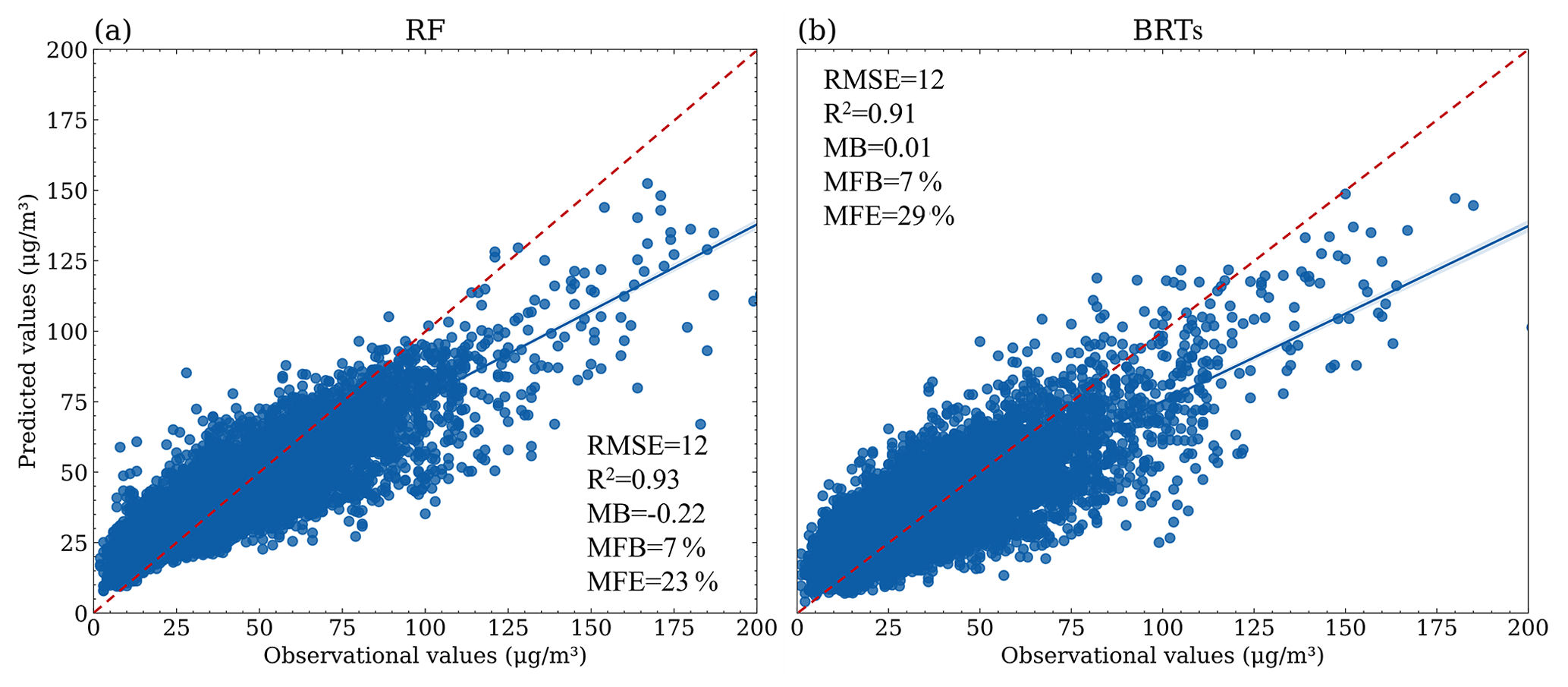
Figure 3The performance of PM2.5 predictions of the two machine learning methods in Guangzhou. (a) RF-deweathered; (b) BRT-deweathered.
The RF algorithm was performed based on the “rmweather” R package (Grange et al., 2018) and the “ranger” R package (Wright and Ziegler, 2017), and the BRTs were performed based on the “deweather” R package (Carslaw et al., 2012; Carslaw and Taylor, 2009). The application of these packages has been well documented in the literature, e.g., analyzing long-term trends in concentrations of air pollutants (Grange and Carslaw, 2019; Ma et al., 2021; Mallet, 2020), assessing the impact of clean-air actions (Vu et al., 2019; Zhang et al., 2020), and evaluating the response of air quality during the COVID-19 lockdown (Dai et al., 2021; Shi and Brasseur, 2020; Wang et al., 2020; Munir et al., 2021; Lovric et al., 2021). The independent input variables to the two machine learning methods include temporal variables (hour, day, weekday, week and month), meteorological parameters (ws, wd, at, rh, dp, blh, tcc, ssr, sp and tp) and monitored pollutant concentrations. The top three most influential meteorological variables in each modeling scenario are listed in Table S3. The inputs were randomly divided into two groups: the training data set that accounts for 80 % of the data and a testing data set that contained the remaining 20 %. The performance was evaluated by statistical metrics, including the correlation coefficient (R2), root mean square error (RMSE), mean bias (MB), mean fractional bias (MFB) and mean fractional error (MFE). The formulas used to calculate RMSE, MB, MFB and MFE are as follows:
in which Pi and Oi represent the ith predicted and observed values, and N represents the number of data used to test. Note that the United States Environmental Protection Agency (USEPA) proposed the criteria and goal values for MFE and MFB to evaluate the air quality modelling performance, which are MFE ≤ 75 % and MFB ≤ ± 60 % for criteria and MFE ≤ 50 % and MFB ≤ ± 30 % for goals (USEPA, 2007). No such criteria value has been set for the other parameters defined in the above equations.
The indices of PM2.5 in Guangzhou are shown as an example in Fig. 3, and the summary of all air pollutants in the six cities can be found in Table S4. In Fig. 3, the minimum RMSE values obtained for the PM2.5 test in Guangzhou and used for the final calculation are 12.1 (RF algorithm) and 12.3 (BRTs), respectively. R2 values are 0.93 (RF algorithm) and 0.91 (BRTs), respectively, implying that the predicted values of PM2.5 by the two methods well reproduce the observations. The MB values are −0.22 (RF algorithm) and 0.01 (BRTs), respectively, implying that the BRTs better reproduced the observations than the RF algorithm in this case. Note that an MB of zero would indicate an ideal prediction. The calculated MB deviating from zero implies that the deweathered hourly concentrations suffer from the errors to some extent, and the errors would automatically transfer into the deweathered trends and PCs. MFB and MFE values were less than 30 % and 50 %, respectively, for both the RF algorithm and BRTs (Fig. 3), satisfying the goal values set by the USEPA. This suggests good performance in reproducing observations using the two methods, as listed in Table S4. Note that the two machine learning methods always underpredicted PM2.5 concentrations in cases with high PM2.5 levels, although such cases occurred infrequently. Such an underprediction has also been reported in air quality model-predicted PM2.5 concentrations, which could be due to missing mechanisms enhancing formation of PM2.5 under poor dispersion conditions (Chang et al., 2020; X. Liu et al., 2021; Zheng et al., 2015; Shen et al., 2022). Under these circumstances, the training for two machine learning methods may not be sufficient to yield good prediction.
In the two machine learning methods, the meteorologically normalized air pollutant concentrations at a particular time were calculated by averaging 1000 model predictions with meteorological variables randomly resampled from the study period (2014–2020), following the approach proposed by Hou et al. (2022).
where xi,pred is the model-predicted concentration for a given meteorological condition at time i, and ydew is the corresponding deweathered hourly concentration at a particular time under an averaged meteorological condition. In this study, the deweathered hourly concentrations by the BRTs contained more spikes than those by the RF method. Some of the spikes may be caused by episodic emissions such as agriculture biomass burning, wild forest fires, holiday fireworks, construction activities (Video S1 in the Supplement) and accidents and associated enhanced secondary pollution (Chen et al., 2017; Dai et al., 2021; Enayati et al., 2021; Chen et al., 2021; Shen et al., 2022). Meteorological data from the nearest airport in every city were used as input for the two machine learning methods, as has been the choice in most existing studies (Vu et al., 2019; Mallet, 2020; Wang et al., 2020; Dai et al., 2021; Ma et al., 2021). The data should reflect synoptic weather conditions and be suitable for modelling hourly pollutant concentrations averaged from multiple sites in a city.
The ICEEMDAN method (Colominas et al., 2014), which is an improved version of the EMD method, overcomes the “end effect” originally existing in EMD, providing modes with less noise and avoiding the spurious modes. The original data can be decomposed and expressed as
where x is the original data, di is the ith intrinsic mode function (IMF), k is the total number of IMFs, and r is the final residual. This method has been applied in various fields, such as financial prediction (Zhou and Chen, 2021) and air quality assessment (Luo et al., 2020). The implementation of the ICEEMDAN method is based on a Python package named PyEMD (Laszuk, 2017). The number of modes needs to be pre-set in this method, which was chosen based on sensitivity test results with the following two criteria: (1) only one oscillation cycle should be kept in the real residual, and (2) combining the real residual and the final mode would end up with two or more oscillation cycles. For example, the decomposed residual plus the last mode was finally used as the real ICEEMDAN-decomposed residual for PM2.5 in Guangzhou, Shenzhen, Zhanjiang and Zhuhai (Fig. S1a–d and f in the Supplement), while the decomposed residual was used directly as the real ICEEMDAN-decomposed residual for PM2.5 in Haikou (Fig. S1e). Note that the ICEEMDAN method requires a complete time series of data. Approximately 5 % of the data were missing for each air pollutant in each city (Table S2), but the missing data did not occur at the identical hour on 2 consecutive days, except for PM10 concentration in Zhanjiang. For the special cases of PM10 in Zhanjiang, the missing data were replaced by the average values of the observed data between the nearest day before and after the identical hour. This approach of replacing missing data may introduce a small uncertainty into the decomposed residuals.
In this study, we also developed a novel method to study emission-driven interannual variations in air pollutant concentrations by calculating the range of DePCs on an annual scale based on an earlier approach proposed by Yao and Zhang (2020) (referring to the self-developed method in the present study). Details of this method are presented in the Supplement, with an example of calculating the range of DePCs of PM2.5 concentration between 2 years (May 2020–April 2021 relative to May 2014–April 2015) in Guangzhou (Table S5 and Fig. S2). There are five steps in this method, including (1) reconstructing the time series of data in any 2 years to the same size, (2) conducting correlation analysis using the reconstructed data in any 2 years and removing outliers after the inflection point (Fig. S2), (3) repeating step (2) to remove more outliers, (4) calculating the range of DePCs and (5) evaluating residual perturbations by varying weather conditions. The main advantages of this method include (1) avoiding the calculation of the deweathered hourly concentrations or decomposed hourly residuals of air pollutants in which their uncertainties are unpredictable, (2) confirming the accuracy of DePCs when the range of DePCs is sufficiently narrow and (3) identifying the large perturbation from varying weather conditions on DePCs when the range of DePCs is broad.
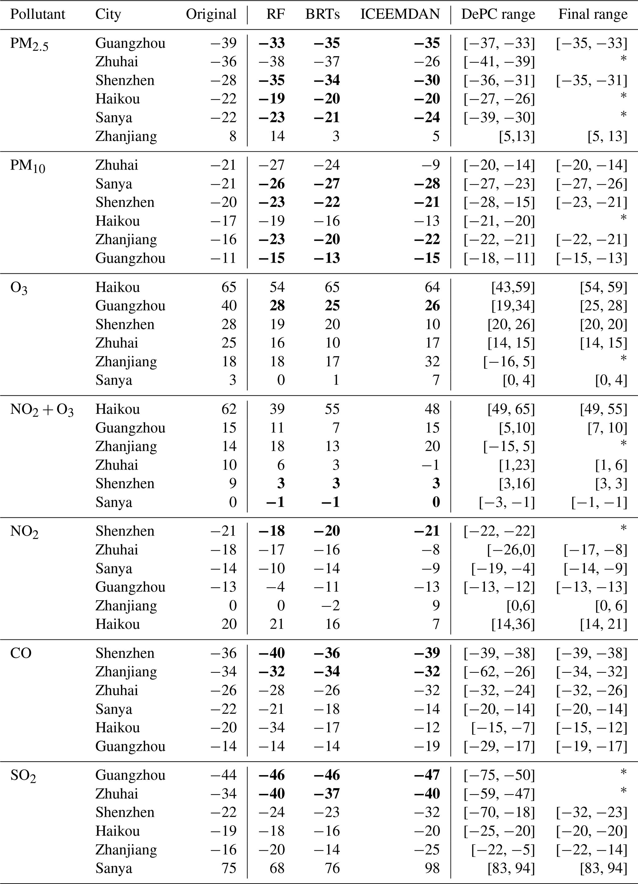
Table 1The original annual average concentrations of six criteria air pollutants and NO2 + O3 and their trends in original annual averages, RF-deweathered and BRT-deweathered concentrations and ICEEMDAN-decomposed residuals in six cities detected by the M–K method. Yellow represents four consistent increasing or decreasing trends, blue represents consistent trends detected only from three methods, green represents consistent trends in original and two machine learning methods.

The M–K analysis is employed to resolve the trends in the time series of the annual average concentration of each pollutant. Qualitative trend results revolved by the M–K method include (1) an increasing/decreasing trend with a P value of < 0.05, (2) a probably increasing/decreasing trend with a P value of 0.05–0.1, (3) a stable trend with a P value of > 0.1 as well as with a ratio of < 1.0 between the standard deviation and the mean of the data set, and (4) no trend for P > 0.1 with all the other conditions (Aziz et al., 2003; Kampata et al., 2008; Yao and Zhang, 2020).
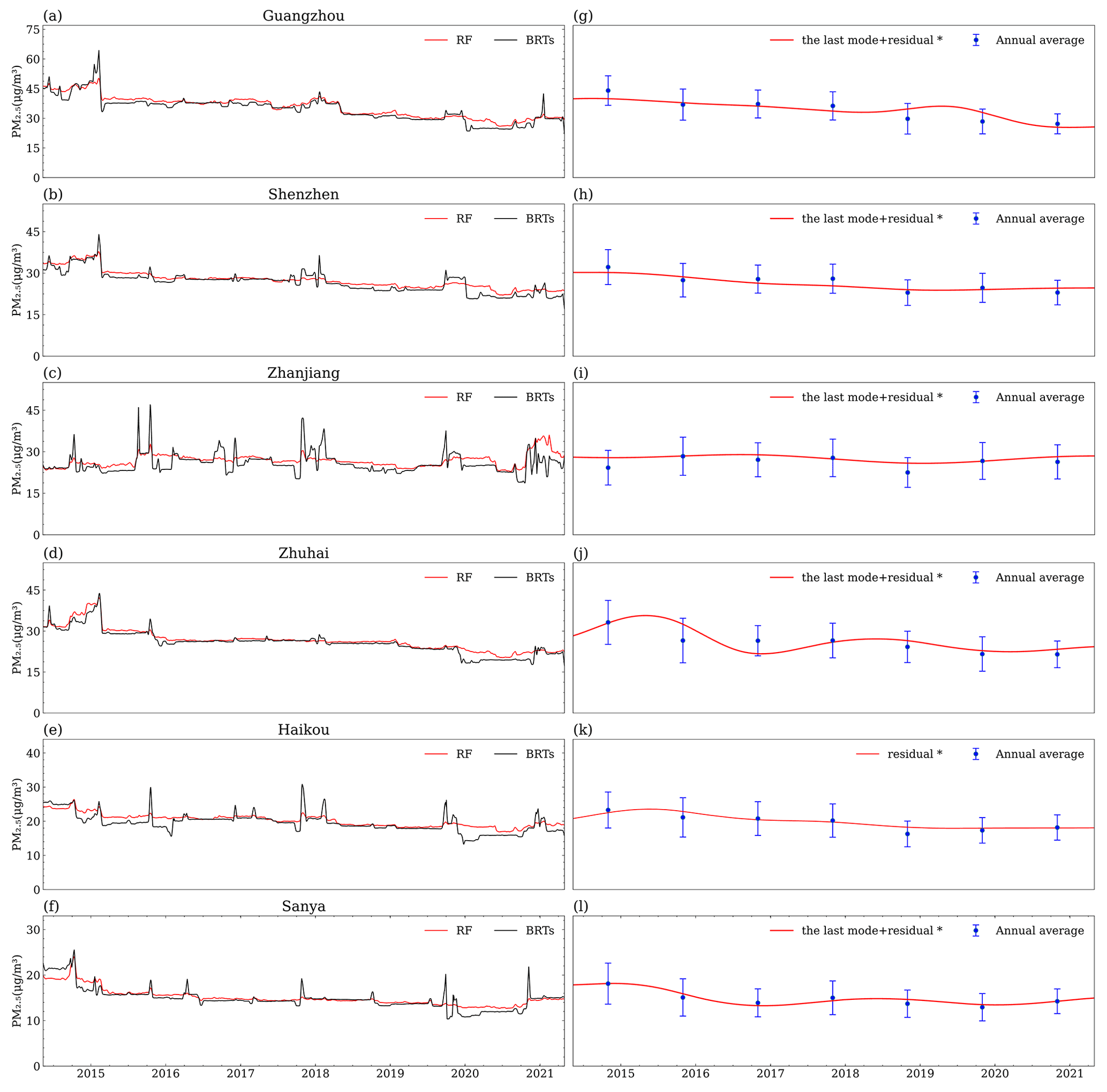
Figure 4The RF-deweathered and BRT-deweathered concentrations and ICEEMDAN-decomposed residuals (or mode + residuals) of PM2.5 and annual averages from May 2014 to April 2021. (a–f) Deweathered concentrations in the six cities (the order of the cities is the same as that listed in Table 1); (g–l) decomposed residual or the last mode + residual and annual averages plus one-third standard deviation in the six cities (∗ represents the time series of values to be used to calculate the trend and PC).
3.1 Trends and PCs of PM2.5 and PM10
The 7-year (2014–2020) average mass concentrations of PM2.5 were the highest in Guangzhou at 34 µg m−3, followed by 27 µg m−3 in Shenzhen, 26 µg m−3 in Zhanjiang and Zhuhai, 20 µg m−3 in Haikou and 15 µg m−3 in Sanya (Table 1). The annual average PM2.5 concentrations in most cities and in nearly all the years (Table S6) exceeded the annual average Class-I level (15 µg m−3) of Ambient Air Quality Standards (AAQS) in China and exceeded the latest WHO air quality guideline values by several times.
The largest decrease in the annual average PM2.5 mass concentration from the first year (2014) to the last year (2020) occurred in Guangzhou, i.e., by 17 µg m−3 (or 39 %) (Table 1 and Fig. 4). A significant decreasing trend was also identified during the 7-year period by the M–K method (p < 0.05). A similar case was also found in Shenzhen with a decrease of 9 µg m−3 (or 28 %) from 2014 to 2020 and a significant decreasing trend (p < 0.05) during the same period. However, a probably decreasing trend (0.05 ≤ p < 0.1) or a stable trend (p ≥ 0.1) was revealed by the M–K method in the other four cities. Note that a 20 %–40 % decrease in PM2.5 annual average concentrations has frequently been observed across China since 2013, e.g., a nationwide decrease by an overall 22 % from 2015 to 2018 (Zhao et al., 2021), an approximately 40 % decrease in Beijing and a 20 % decrease in the Pearl River Delta from 2015 to 2019 (Hu et al., 2021; Xu and Zhang, 2020).
Table 2The PCs of six criteria pollutants and NO2 + O3 calculated from original averages, RF-deweathered and BRT-deweathered concentrations and ICEEMDAN-decomposed residuals and the robust ranges of DePC in six cities (units: %; ∗ represents no robust DePC). The bolded numbers represent consistent PCs calculated from three methods.
To explore the emission-driven trends in PM2.5 concentration in the six cities, the RF-deweathered and BRT-deweathered PM2.5 concentrations and the ICEEMDAN-decomposed residuals of PM2.5 concentrations are examined in Fig. 4a–l. In Guangzhou and Shenzhen, a consistent decreasing trend (p < 0.05) was identified by the M–K method in the deweathered PM2.5 concentrations and the decomposed residuals of PM2.5 concentrations (Table 1 and Fig. 4a and b). The PCs from 2014 to 2020 were also reasonably consistent between the different data sets mentioned above (Table 2), i.e., with the standard deviation of the three PCs being within 10 % of the corresponding mean absolute value. Specifically, the PCs from 2014 to 2020 in Shenzhen calculated from the RF-deweathered and BRT-deweathered PM2.5 concentrations and the ICEEMDAN-decomposed residuals were −35 %, −34 % and −30 %, respectively, which were not much different from that using the original PM2.5 concentration (28 % as discussed above). A combination of these four PC values in Shenzhen allowed us to infer that (1) the reduced air pollutant emissions in Shenzhen and upwind regions likely decreased the PM2.5 concentrations by 33 % ± 3 % (mean ± standard deviation) from 2014 to 2020, and (2) the perturbation from varying weather conditions cancelled out 5 % ± 3 % out of the 33 % ± 3 % decrease. In Guangzhou, the PCs of PM2.5 concentrations from 2014 to 2020 estimated by the three methods were −33 % (RF-deweathered), −35 % (BRT-deweathered) and −35 % (ICEEMDAN-decomposed), while the PCs calculated from the original annual average PM2.5 concentrations was −39 %, as mentioned above. Thus, the reduced emissions of air pollutants in Guangzhou and upwind regions likely decreased the concentrations of PM2.5 by 34 % ± 1 % during the 7-year period, while the perturbation from varying weather conditions caused an additional decrease of 5 % ± 1 %. Gong et al. (2021) also reported an additional 5 % decrease driven by varying meteorological conditions, on top of the 47 % decrease driven by reduced emissions, in the national annual averages of PM2.5 mass concentration from 2013 to 2019 in China.
A decreasing trend (p < 0.05) was also identified in Zhuhai, Haikou and Sanya when using the RF-deweathered and BRT-deweathered concentrations and the ICEEMDAN-decomposed residuals (Table 1 and Fig. 4d, e, and j–l), which are in contrast with probably decreasing trends generated from using the original PM2.5 concentration data. The perturbations from varying weather conditions on PM2.5 mass concentrations likely complicated the effects of reduced air pollutant emissions in the three cities and upwind regions during 2014–2020. It is noted that the PCs estimated from the three different methods (RF-deweathered, BRT-deweathered and ICEEMDAN-decomposed) varied little for Sanya (−23 %, −21 % and −24 %) and Haikou (−19 %, −20 % and −20 %) from 2014 to 2020 but were quite large for Zhuhai (−38 %, −37 % and −26 %); the latter case was likely due to the large uncertainties associated with one or more methods (Table 2). We revealed the most influential meteorological factors in the RF-predicted and BRT-predicted concentrations, which was surface pressure in 7 out of 12 cases, followed by relative humidity in 3 out of 12 cases, dew point in 1 case, and air temperature in 1 case (Table S3). However, the influence of surface pressure on pollutant concentrations was poorly understood, and so is the case of its role in interpreting uncertainties in modelling results.
No trend or a stable trend was identified for Zhanjiang (Table 1, Fig. 4c and i), regardless of which method was used. The PCs from 2014 to 2020 were all positive, i.e., 14 % (RF-deweathered), 3 % (BRT-deweathered), 5 % (ICEEMDAN-decomposed), and 8 % (original data), indicating emission-driven increases in PM2.5 concentration in this city during this period.
A similar analysis to the one discussed above was also conducted on PM10 concentrations (Tables 1 and 2 and Fig. S3a–l), the results of which can be summarized below.
-
The highest 7-year (2014–2020) average PM10 concentrations of 57 µg m−3 occurred in Guangzhou, followed by 45 µg m−3 in Shenzhen, 43 µg m−3 in Zhuhai, 42 µg m−3 in Zhanjiang, 37 µg m−3 in Haikou and 29 µg m−3 in Sanya. The annual average PM10 concentrations exceeded the annual average Class-I level (40 µg m−3) of AAQS in China in most cities and most years and exceeded the latest WHO air quality guideline values by 2–4 times.
-
The M–K analyses showed either no or a stable trend during 2014–2020 when using the original annual average PM10 concentrations in the six cities (Table 1). Inconsistent trends were then obtained by using the three different methods (RF-deweathered, BRT-deweathered and ICEEMDAN-decomposed) in five out of the six cities. The only exception is for Guangzhou, in which a decreasing trend was identified from all three methods, although no trend was extracted from the original annual average concentrations. For Shenzhen, a decreasing trend was obtained using the RF-deweathered method, while a probably decreasing or stable trend was obtained from the BRT-deweathered and ICEEMDAN-decomposed method. For Sanya, a decreasing trend was obtained using the RF-deweathered and ICEEMDAN-decomposed methods, while no trend was obtained using the BRT-deweathered method. The inconsistency between the trends extracted by the three different methods was mostly because the actual interannual changes, and thus the magnitudes of the trends, were small, which are on the same order of magnitude as the methodology uncertainties. Combining all the trends generated using the three different methods and the original data, we concluded a slightly decreasing or stable trend in emission-driven PM10 concentrations for all the cities.
-
The PCs of PM10 concentration from 2014 to 2020 in Guangzhou were consistent between using the three different methods, e.g., −15 % (RF-deweathered), −13 % (BRT-deweathered) and −15 % (ICEEMDAN-decomposed), and that from using the original PM10 concentration data, −11 %. Thus, reduced emissions of air pollutants in Guangzhou and upwind regions likely decreased PM10 concentrations by 14 % ± 1 % during the 7-year period, while the perturbation from varying weather conditions cancelled out 3 % ± 1 %. The reasonably consistent PCs were also obtained for Shenzhen, Zhanjiang and Sanya, although with inconsistent decreasing trends. However, inconsistent PCs were obtained from the three different methods for the other three cities due to methodology uncertainties and the actual small trends, as explained above.
3.2 Trends and PCs of O3, NO2 and NO2 + O3
Among the four gaseous criteria pollutants, O3 concentrations in the six cities exceeded the most, on a percentage basis, the Class-I levels of AAQS in China (Table S6). Trend analyses were conducted for both O3 and NO2 + O3 considering the titration reaction of O3 with NO to form NO2 in ambient air (Chan and Yao, 2008; K. Li et al., 2019; Seinfeld and Pandis, 1998; Sicard et al., 2020; Wang et al., 2017).
The 7-year (2014–2020) average concentrations of O3 were highest at 69 µg m−3 in Zhanjiang and Zhuhai, followed by 62 µg m−3 in Shenzhen, 60 µg m−3 in Haikou, 58 µg m−3 in Sanya (Table 1), and 51 µg m−3 in Guangzhou. The titration reaction of O3 with NO likely decreased O3 concentrations to some extent in Guangzhou, as implied by the highest annual average NO2 concentrations in this city among the six cities (Table 1). In contrast, the highest O3 annual averages occurred in Zhanjiang and Zhuhai. The annual average NO2 concentrations in the two cities were smaller than that in Guangzhou but larger than that in Sanya. Thus, both the reduced depletion of O3 via the titration reaction and the enhanced photochemical formation of O3 likely contributed to the highest annual average O3 concentrations in the two cities (G. He et al., 2021; X. F. Liu et al., 2021; Shen et al., 2021).
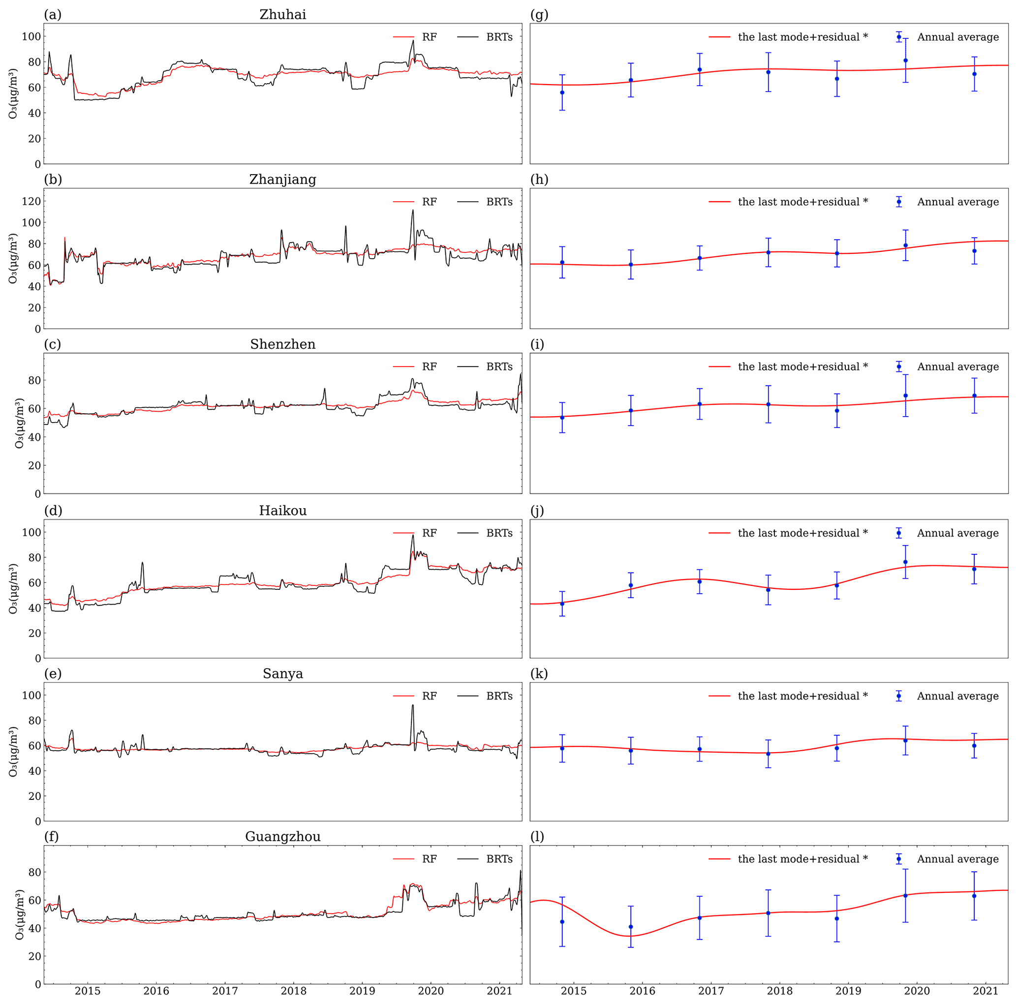
Using the original data of annual average O3 concentrations (Table 1 and Fig. 5a–f), the M–K analysis results showed an increasing trend in Zhanjiang, Shenzhen, Haikou and Guangzhou (p < 0.05) and no trend in Zhuhai and Sanya. Using the RF-deweathered concentrations, the BRT-deweathered concentrations and the ICEEMDAN-decomposed residuals (Figs. 5a–l and S1g–l), M–K analysis results generated the same trend as mentioned above in every city. Thus, the emission-driven increasing trends in O3 concentration from 2014 to 2020 can be firmly confirmed in four cities (Zhanjiang, Shenzhen, Haikou and Guangzhou).
The PCs of the deweathered concentrations, the decomposed residuals, and the original annual average concentrations from 2014 to 2020 in the four cities with increasing trends of O3 concentration were further analyzed and were presented below from the largest to the smallest PCs. In Haikou, the PC from 2014 to 2020 was 65 % based on the original annual average O3 concentrations (Table 2). The corresponding PCs were 54 %, 65 % and 64 % based on the RF-deweathered concentrations, the BRT-deweathered concentrations, and the ICEEMDAN-decomposed residuals, respectively. Combining these numbers together, we concluded that the emission changes in O3 precursors and associated changes in atmospheric chemistry likely increased the O3 concentration by at least 54 % from 2014 to 2020, and the perturbations from varying weather conditions seemingly yielded an additional increase of 0 %–11 %. Similarly, in Guangzhou, Shenzhen and Zhanjiang, the emission changes in O3 precursors likely increased the concentrations of O3 by 26 % ± 1.5 %, > 10 % and > 17 %, respectively, from 2014 to 2020, and the perturbations from varying weather conditions seemingly yielded additional increases of 14 % ± 1.5 %, 8 %–18 % and −1 %–14 %, respectively.
In the case of NO2, Guangzhou is the only city with annual average NO2 concentrations exceeding the annual average Class-I level of AAQS in China (40 µg m−3) in most of the years; the only exception is in 2020, mostly due to reduced emissions as a result of the COVID-19 pandemic (Bauwens et al., 2020; Shi and Brasseur, 2020; Wang et al., 2020; Wang et al., 2021; Zhao et al., 2020). Annual average NO2 concentrations were below 40 µg m−3 in all the other cities during all the years but were far above the latest WHO air quality guideline value of 10 µg m−3. When the 7-year (2014−2020) average NO2 concentrations in six cities were compared, the value of 46 µg m−3 in Guangzhou ranked at the top, followed by 30 µg m−3 in Shenzhen, 29 µg m−3 in Zhuhai, 15 µg m−3 in Zhanjiang and Haikou, and 12 µg m−3 in Sanya (Table 1).
A decreasing trend in NO2 concentration from 2014 to 2020 was obtained in Shenzhen and Zhuhai based on the deweathered concentrations and the decomposed residuals, while a probably decreasing trend was obtained based on the original annual average concentration data (Fig. S5a–l). In Shenzhen, the PCs in NO2 from 2014 to 2020 were mostly consistent between the different methods (Table 2), e.g., −18 % (RF-deweathered), −20 % (BRT-deweathered), −21 % (ICEEMDAN-decomposed) and −21 % (original data). However, this was not the case in Zhuhai, for which the four PCs were −17 % (RF-deweathered), −16 % (BRT-deweathered), −8 % (ICEEMDAN-decomposed) and −18 % (original annual average). A stable trend in NO2 concentration from 2014 to 2020 was obtained in Guangzhou, regardless of the method used. The impact of the reduced NOx emissions in Guangzhou and/or upwind areas could not be detected in the observed NO2 concentrations on the annual scale. Inconsistent trends were obtained between using different methods in Zhanjiang, Haikou and Sanya, similar to the cases of several other pollutants discussed above and below.
Combining NO2 and O3 together, an increasing trend (p < 0.05, Table 2) was obtained from 2014 to 2020 in Haikou, while probably increasing no trend or stable trends were obtained in the other five cities based on the original annual average concentration data (Fig. S4a–l). A consistent increasing trend in NO2 + O3 was obtained in Guangzhou and Zhanjiang based on any of the RF-deweathered concentrations, BRT-deweathered concentrations, and decomposed residuals of NO2 + O3. In Haikou, an increasing trend was obtained based on the RF-deweathered and BRT-deweathered concentrations, while a probably increasing trend was obtained from the decomposed residuals. The increasing trends in NO2 + O3 from 2014 to 2020 in the above-mentioned three cities confirmed the enhanced formation of O3. However, either no or stable trends were obtained in Zhuhai, Shenzhen and Sanya based on the deweathered concentrations or the decomposed residuals of NO2 + O3 (Table 1). The contrasting trends between NO2 + O3 and O3 in Shenzhen, i.e., no trend in the former and an increasing trend in the latter (Table 1), were likely due to the reduced O3 depletion via the titration reaction of O3 by NO.
The PCs in NO2 + O3 from 2014 to 2020 in Haikou, Guangzhou and Zhanjiang were presented below from the largest to the smallest PCs. In Haikou, the PCs were estimated to be 39 %, 55 %, 48 % and 62 % based on the RF-deweathered concentrations, the BRT-deweathered concentrations, the ICEEMDAN-decomposed residual and the original annual average concentrations, respectively. Thus, the 39 %−55 % O3 increases from 2014 to 2020 were likely attributed to the emission-driven enhanced O3 formation. In addition, the first three PC values for NO2 + O3 were smaller than those of O3 by 10 %−16 %, which represented the reduced O3 depletion via the titration reaction (K. Li et al., 2019; Wang et al., 2017). In Guangzhou, the estimated four PCs in NO2 + O3 were 11 % (RF-deweathered), 7 % (BRT-deweathered), 15 % (ICEEMDAN-decomposed) and 15 % (original data). These numbers were smaller than those for O3 by 11 %−25 %, implying similar contributions from the reduced O3 depletion via the titration reaction and the enhanced O3 formation to the total increased O3 concentration. In Zhanjiang, the estimated four PCs in NO2 + O3 were 18 %, 13 %, 20 % and 14 %, which are mostly similar to those for O3 (18 %, 17 %, 32 % and 18 %) (Table 2), implying the dominant contribution of the enhanced O3 formation to the increased O3 concentration.
3.3 Trends and PCs of CO and SO2
The annual average concentrations of CO and SO2 were all below the Class-I levels of AAQS in China during 2014–2020 in all the cities (Table 1). A consistent decreasing trend in annual average CO concentration was obtained, regardless of which method was used, in all the cities except Haikou (Fig. S6a–l). A consistent decreasing trend in annual average SO2 concentration was also obtained using the four different methods in Shenzhen and Zhuhai. In Guangzhou, a decreasing trend in annual average SO2 concentration was obtained based on the deweathered concentrations and decomposed residuals, while a probably decreasing trend was obtained based on the original annual average data (Fig. S7a–l). In Sanya, an increasing trend in annual average SO2 concentration was obtained based on the deweathered concentrations and decomposed residuals, while a probably increasing trend was obtained based on the original annual average data. In Haikou and Zhanjiang, inconsistent trends were obtained between using the deweathered concentrations and decomposed residuals.
The reasonably consistent PCs in annual average CO concentrations from 2014 to 2020 between using different methods were only obtained in Shenzhen and Zhanjiang, i.e., −40 % and −32 % (RF-deweathered), −36 % and −34 % (BRT-deweathered), −39 % and −32 % (ICEEMDAN-decomposed), and −36 % and −34 % (original data), respectively. The PCs in SO2 from 2014 to 2020 were reasonably consistent between using different methods in Guangzhou and Zhuhai; e.g., the four values in Guangzhou were −46 % (RF-deweathered), −46 % (BRT-deweathered), −47 % (ICEEMDAN-decomposed) and −44 % (original average).
3.4 Constraining analysis uncertainties
Of the 42 cases analyzed in this study, approximately 70 % showed consistent trends from 2014 to 2020 between using the RF-deweathered concentrations, the BRT-deweathered concentrations and the ICEEMDAN-decomposed residuals as input to the M–K analysis. The remaining 30 % with inconsistent trends were apparently caused by methodology uncertainties in some or all of the three methods (RF, BRTs and ICEEMDAN). The PCs from 2014 to 2020 using the same three data sets, although mostly comparable, were only absolutely consistent in approximately 30 % of the cases. Thus, the PCs calculated from the above three methods were further assessed using the range of DePCs using the self-developed method introduced in Sect. 2. Even for the consistent cases, additional examination using an independent method is still valuable for excluding potential coincidence.
The PCs of PM2.5 from 2014 to 2020 varied from −35 % to −33 % in Guangzhou and from −35 % to −30 % in Shenzhen as discussed in Sect. 3. After applying the self-developed method, the corresponding DePCs were estimated to be in the ranges of −37 % to −33 % in Guangzhou and −36 % to −31 % in Shenzhen. The overlap portion between the range of PCs and the range of DePCs in each city was thereby set up as the robust range of DePCs, i.e., −35 % to −33 % in Guangzhou and −35 % to −31 % in Shenzhen (Table 2). The robust ranges of DePCs were almost the same as those of PCs in both cities, further confirming the emission-driven PCs and the perturbation from varying weather conditions presented in Sect. 3. These cases were referred to as Category 1-a below.
The PCs of PM2.5 from 2014 to 2020 were from −20 % to −19 % in Haikou and from −24 % to −21 % in Sanya. The corresponding DePCs had no overlap with these PC ranges in these cities, implying the non-existence of a robust range of DePCs. These cases were referred to as Category 1-b below. Note that the self-developed method would not introduce additional observational variables in the calculation process as shown in Sect. S1 in the Supplement and Fig. S2, and the true DePC should be within the range of DePCs calculated using the self-developed method. The consistent results obtained from the deweathered concentrations and decomposed residuals in Category 1-b were likely ascribed to a coincidence and may be invalid.
The PCs of PM2.5 from 2014 to 2020 were in a relatively large range in Zhuhai and Zhanjiang, implying a certain extent of inconsistency between the three methods (RF, BRTs, and ICEEMDAN). The PCs in Zhuhai varied from −38 % to −26 %, and the corresponding DePC had no overlap with this range, implying the non-existence of a robust range of DePC. This case was referred to as Category 2-a below. Similar to Category 1-b, the deweathered and decomposed methods cannot reasonably estimate the perturbation from varying weather conditions in Category 2-a. The PCs in Zhanjiang ranged from 3 % to 14 %, and the corresponding DePC completely overlapped this range, again confirming the emission-driven PCs and the perturbation from varying weather conditions presented in Sect. 3. This case was referred to as Category 2-b below.
The PCs of PM10 from 2014 to 2020 were inconsistent between using the RF-deweathered concentrations, the BRT-deweathered concentrations and the ICEEMDAN-decomposed residuals of PM10 in Zhuhai. Nevertheless, a robust range of DePCs was obtained in Zhuhai (−20 % to −14 %). Comparing the robust range of DePCs with the range of PCs calculated using the original annual average data (−21 %), the perturbation from varying weather conditions yielded an additional decrease in PM10 concentration by 1 %–7 % in Zhuhai. This case was referred to as Category 2-c below, featuring a narrower robust range of DePCs than that of PCs calculated from the deweathered concentrations and decomposed residuals. PM10 in Sanya, Shenzhen, Zhanjiang and Guangzhou followed into Category 1-a, confirming the emission-driven PCs and the perturbation from varying weather conditions. PM10 in Haikou followed into Category 2-a with no robust range of DePCs.
O3 in Haikou, Shenzhen and Zhuhai followed into Category 2-c, and that in Guangzhou, Zhanjiang and Sanya followed into Categories 1-a, 2-a and 2-b, respectively. Results of NO2 + O3, NO2, CO and SO2 also followed into some of the five categories (Table 2), and the above interpretation for PM2.5, PM10 and O3 in each category on the emission-driven PCs and the perturbation from varying weather conditions are also applicable to NO2 + O3, NO2, CO and SO2.
In this study, we first applied separately the RF algorithm, the BRT algorithm, and the ICEEMDAN to obtain time series of the deweathered concentrations or decomposed residuals of criteria air pollutants and NO2 + O3 from May 2014 to April 2021 in the six cities in South China. We found that the RF-deweathered and BRT-deweathered concentrations and the ICEEMDAN-decomposed residuals yielded consistent trends in approximately 70 % of the cases. We then calculated the PCs between the first and last years using the above-mentioned deweathered concentrations and residuals. Only in approximately 30 % of the cases were the PCs reasonably consistent between the three methods, indicating large methodology uncertainties in one or more methods. The self-developed method was further used to calculate the range of DePCs, and a robust range of DePCs was identified in approximately 70 % of the cases.
Based on those consistent trends obtained from the different methods and the robust range of DePCs, we finally generated the following findings.
-
Significant decreasing trends in PM2.5 concentration during 2014–2020 were identified in Guangzhou and Shenzhen, which were mainly caused by the reduced air pollutant emissions and to a much lesser extent by weather perturbations. A stable or no trend in PM2.5 was identified in Zhanjiang, implying no detectable effects of the reduced air pollutant emissions on the monitored PM2.5. Decreasing or probably decreasing emission-driven trends were obtained in the remaining cities. The emission-driven effects likely took the lead in the overall changes, although uncertainties associated with one or more methods still existed on the basis of inconsistent PCs.
-
Increasing trends in O3 concentration during 2014–2020 were identified in Zhanjiang, Shenzhen, Guangzhou and Haikou. The emission changes in O3 precursors played a more dominant role than did the perturbations from varying weather conditions. However, increasing trends in NO2 + O3 were only identified in Zhanjiang, Guangzhou and Haikou with increasing and probably increasing trends obtained from different methods, which also confirmed the different contribution ratios of the reduced O3 depletion via the titration reaction and the enhanced formation of O3.
This study demonstrates the necessity of combining multiple decoupling and/or trend analysis methods in order to constrain the uncertainties in trend analysis results inherent in any individual method. Interpretation of trend analysis results presented in this study could be strengthened if detailed discussions of atmospheric processes and chemistry mechanisms were provided, which unfortunately could not be accommodated here due to the lack of reliable long-term data on the concerned chemical species, such as the major chemical components in PM2.5 and PM10, VOCs and an up-to-date emission inventory of all the involved pollutants. A lack of knowledge of the detailed city-level mitigation measures on air pollutants also limited our capacity to provide a comprehensive assessment of the existing clean-air policies.
The code of DePC calculation can be accessed via https://pypi.org/project/DePC/ (Lin, 2022), and the data used in this paper are downloadable from http://www.cnemc.cn/sssj/ (China National Environmental Monitoring Centre, 2010).
The supplement related to this article is available online at: https://doi.org/10.5194/acp-22-16073-2022-supplement.
XY and LZ designed the research. YL and QF carried out the measurement and analyzed the data. All the authors provided comments and contributed to the text.
At least one of the (co-)authors is a member of the editorial board of Atmospheric Chemistry and Physics. The peer-review process was guided by an independent editor, and the authors also have no other competing interests to declare.
Publisher's note: Copernicus Publications remains neutral with regard to jurisdictional claims in published maps and institutional affiliations.
This work was supported by the Hainan Provincial Natural Science Foundation of China (grant no. 422MS098), the Natural Science Foundation of China (grant no. 41776086) and the Hainan Provincial Postgraduate Innovative Research Project (grant no. Yhys2021-5).
This research has been supported by the Hainan Provincial Natural Science Foundation of China (grant no. 422MS098), the Natural Science Foundation of China (grant no. 41776086) and the Hainan Provincial Postgraduate Innovative Research Project (grant no. Yhys2021-5).
This paper was edited by Rob MacKenzie and reviewed by Zongbo Shi and one anonymous referee.
Astitha, M., Luo, H., Rao, S. T., Hogrefe, C., Mathur, R., and Kumar, N.: Dynamic evaluation of two decades of WRF-CMAQ ozone simulations over the contiguous United States, Atmos. Environ., 164, 102–116, https://doi.org/10.1016/j.atmosenv.2017.05.020, 2017.
Aziz, J. J., Ling, M., Rifai, H. S., Newell, C. J., and Gonzales, J. R.: MAROS: a decision support system for optimizing monitoring plans, Ground Water, 41, 355–367, https://doi.org/10.1111/j.1745-6584.2003.tb02605.x, 2003.
Bauwens, M., Compernolle, S., Stavrakou, T., Muller, J. F., van Gent, J., Eskes, H., Levelt, P. F., van der, A. R., Veefkind, J. P., Vlietinck, J., Yu, H., and Zehner, C.: Impact of coronavirus outbreak on NO2 pollution assessed using TROPOMI and OMI observations, Geophys. Res. Lett., 47, e2020GL087978, https://doi.org/10.1029/2020GL087978, 2020.
Borlaza, L. J., Weber, S., Marsal, A., Uzu, G., Jacob, V., Besombes, J.-L., Chatain, M., Conil, S., and Jaffrezo, J.-L.: Nine-year trends of PM10 sources and oxidative potential in a rural background site in France, Atmos. Chem. Phys., 22, 8701–8723, https://doi.org/10.5194/acp-22-8701-2022, 2022.
Carslaw, D. C.: Worldmet: Import Surface Meteorological Data from NOAA Integrated Surface Database (ISD), R package version 0.9.5, https://cran.r-project.org/package=worldmet (last access: 13 December 2022), 2021.
Carslaw, D. C. and Taylor, P. J.: Analysis of air pollution data at a mixed source location using boosted regression trees, Atmos. Environ., 43, 3563–3570, https://doi.org/10.1016/j.atmosenv.2009.04.001, 2009.
Carslaw, D. C., Williams, M. L., and Barratt, B.: A short-term intervention study — Impact of airport closure due to the eruption of Eyjafjallajökull on near-field air quality, Atmos. Environ., 54, 328–336, https://doi.org/10.1016/j.atmosenv.2012.02.020, 2012.
Chan, C. K. and Yao, X. H.: Air pollution in mega cities in China, Atmos. Environ., 42, 1–42, https://doi.org/10.1016/j.atmosenv.2007.09.003, 2008.
Chang, Y., Huang, R. J., Ge, X., Huang, X., Hu, J., Duan, Y., Zou, Z., Liu, X., and Lehmann, M. F.: Puzzling Haze Events in China During the Coronavirus (COVID-19) Shutdown, Geophys. Res. Lett., 47, e2020GL088533, https://doi.org/10.1029/2020GL088533, 2020.
Chen, J., Li, C., Ristovski, Z., Milic, A., Gu, Y., Islam, M. S., Wang, S., Hao, J., Zhang, H., He, C., Guo, H., Fu, H., Miljevic, B., Morawska, L., Thai, P., Lam, Y. F., Pereira, G., Ding, A., Huang, X., and Dumka, U. C.: A review of biomass burning: Emissions and impacts on air quality, health and climate in China, Sci. Total Environ., 579, 1000–1034, https://doi.org/10.1016/j.scitotenv.2016.11.025, 2017.
Chen, L., Zhu, J., Liao, H., Yang, Y., and Yue, X.: Meteorological influences on PM2.5 and O3 trends and associated health burden since China's clean air actions, Sci. Total Environ., 744, 140837, https://doi.org/10.1016/j.scitotenv.2020.140837, 2020.
Chen, X. K., Jiang, Z., Shen, Y. N., Li, R., Fu, Y. F., Liu, J., Han, H., Liao, H., Cheng, X. G., Jones, D. B. A., Worden, H., and González Abad, G.: Chinese regulations are working – why is surface ozone over industrialized areas still high? Applying lessons from Northeast US air quality evolution, Geophys. Res. Lett., 48, e2021GL092816, https://doi.org/10.1029/2021gl092816, 2021.
China National Environmental Monitoring Centre: Real time data of urban air quality, CNEMC [data set], http://www.cnemc.cn/sssj/ (last access: 13 December 2022), 2010.
Colominas, M. A., Schlotthauer, G., and Torres, M. E.: Improved complete ensemble EMD: A suitable tool for biomedical signal processing, Biomed. Signal Proces., 14, 19–29, https://doi.org/10.1016/j.bspc.2014.06.009, 2014.
Dai, Q. L., Hou, L. L., Liu, B. W., Zhang, Y. F., Song, C. B., Shi, Z. B., Hopke, P. K., and Feng, Y. C.: Spring Festival and COVID-19 lockdown:disentangling PM sources in major Chinese cities, Geophys. Res. Lett., 48, e2021GL093403, https://doi.org/10.1029/2021gl093403, 2021.
Dang, R. J., Liao, H., and Fu, Y.: Quantifying the anthropogenic and meteorological influences on summertime surface ozone in China over 2012–2017, Sci. Total Environ., 754, 142394, https://doi.org/10.1016/j.scitotenv.2020.142394, 2021.
Enayati, A. F., Pakbin, P., Hasheminassab, S., Epstein, S. A., Li, X., Polidori, A., and Low, J.: Long-term trends of PM2.5 and its carbon content in the South Coast Air Basin: A focus on the impact of wildfires, Atmos. Environ., 255, 118431, https://doi.org/10.1016/j.atmosenv.2021.118431, 2021.
Foley, K. M., Hogrefe, C., Pouliot, G., Possiel, N., Roselle, S. J., Simon, H., and Timin, B.: Dynamic evaluation of CMAQ part I: Separating the effects of changing emissions and changing meteorology on ozone levels between 2002 and 2005 in the eastern US, Atmos. Environ., 103, 247–255, https://doi.org/10.1016/j.atmosenv.2014.12.038, 2015.
Fu, H. Y., Zhang, Y. T., Liao, C., Mao, L., Wang, Z. Y., and Hong, N. N.: Investigating PM2.5 responses to other air pollutants and meteorological factors across multiple temporal scales, Sci. Rep.-UK, 10, 15639, https://doi.org/10.1038/s41598-020-72722-z, 2020.
Gong, S., Liu, H., Zhang, B., He, J., Zhang, H., Wang, Y., Wang, S., Zhang, L., and Wang, J.: Assessment of meteorology vs. control measures in the China fine particular matter trend from 2013 to 2019 by an environmental meteorology index, Atmos. Chem. Phys., 21, 2999–3013, https://doi.org/10.5194/acp-21-2999-2021, 2021.
Grange, S. K. and Carslaw, D. C.: Using meteorological normalisation to detect interventions in air quality time series, Sci. Total Environ., 653, 578–588, https://doi.org/10.1016/j.scitotenv.2018.10.344, 2019.
Grange, S. K., Carslaw, D. C., Lewis, A. C., Boleti, E., and Hueglin, C.: Random forest meteorological normalisation models for Swiss PM10 trend analysis, Atmos. Chem. Phys., 18, 6223–6239, https://doi.org/10.5194/acp-18-6223-2018, 2018.
He, G., Deng, T., Wu, D., Wu, C., Huang, X. F., Li, Z. N., Yin, C. Q., Zou, Y., Song, L., Ouyang, S. S., Tao, L. P., and Zhang, X.: Characteristics of boundary layer ozone and its effect on surface ozone concentration in Shenzhen, China: A case study, Sci. Total Environ., 791, 148044, https://doi.org/10.1016/j.scitotenv.2021.148044, 2021.
He, J. J., Gong, S. L., Yu, Y., Yu, L. J., Wu, L., Mao, H. J., Song, C. B., Zhao, S. P., Liu, H. L., Li, X. Y., and Li, R. P.: Air pollution characteristics and their relation to meteorological conditions during 2014-2015 in major Chinese cities, Environ. Pollut., 223, 484–496, https://doi.org/10.1016/j.envpol.2017.01.050, 2017.
He, K. B., Huo, H., and Zhang, Q.: Urban Air Pollution in China: Current Status, Characteristics, and Progress, Annu. Rev. Energ. Env., 27, 397–431, https://doi.org/10.1146/annurev.energy.27.122001.083421, 2002.
He, Y. X., Pan, Y. P., Gu, M. N., Sun, Q., Zhang, Q. Q., Zhang, R. J., and Wang, Y. S.: Changes of ammonia concentrations in wintertime on the North China Plain from 2018 to 2020, Atmos. Res., 253, 105490, https://doi.org/10.1016/j.atmosres.2021.105490, 2021.
Henneman, L. R. F., Holmes, H. A., Mulholland, J. A., and Russell, A. G.: Meteorological detrending of primary and secondary pollutant concentrations: Method application and evaluation using long-term (2000–2012) data in Atlanta, Atmos. Environ., 119, 201–210, https://doi.org/10.1016/j.atmosenv.2015.08.007, 2015.
Hogrefe, C., Rao, S. T., Zurbenko, I. G., and Porter, P. S.: Interpreting the Information in Ozone Observations and Model Predictions Relevant to Regulatory Policies in the Eastern United States, B. Am. Meteorol. Soc., 81, 2083–2106, https://doi.org/10.1175/1520-0477(2000)081<2083:itiioo>2.3.co;2, 2000.
Hogrefe, C., Vempaty, S., Rao, S. T., and Porter, P. S.: A comparison of four techniques for separating different time scales in atmospheric variables, Atmos. Environ., 37, 313–325, https://doi.org/10.1016/S1352-2310(02)00897-X, 2002.
Hou, L. L., Dai, Q. L., Song, C. B., Liu, B. W., Guo, F. Z., Dai, T. J., Li, L. X., Liu, B. S., Bi, X. H., Zhang, Y. F., and Feng, Y. C.: Revealing Drivers of Haze Pollution by Explainable Machine Learning, Environ. Sci. Tech. Let., 9, 112–119, https://doi.org/10.1021/acs.estlett.1c00865, 2022.
Hu, M. M., Wang, Y. F., Wang, S., Jiao, M. Y., Huang, G. H., and Xia, B. C.: Spatial-temporal heterogeneity of air pollution and its relationship with meteorological factors in the Pearl River Delta, China, Atmos. Environ., 254, 118415, https://doi.org/10.1016/j.atmosenv.2021.118415, 2021.
Kampata, J. M., Parida, B. P., and Moalafhi, D. B.: Trend analysis of rainfall in the headstreams of the Zambezi River Basin in Zambia, Phys. Chem. Earth, 33, 621–625, https://doi.org/10.1016/j.pce.2008.06.012, 2008.
Laszuk, D.: PyEMD: Python implementation of Empirical Mode Decomposition algorithm, Python package version 1.2.0, https://pypi.org/project/EMD-signal/ (last access: 13 December 2022), 2017.
Li, K., Jacob, D. J., Liao, H., Shen, L., Zhang, Q., and Bates, K. H.: Anthropogenic drivers of 2013–2017 trends in summer surface ozone in China, P. Natl. Acad. Sci. USA, 116, 422–427, https://doi.org/10.1073/pnas.1812168116, 2019.
Li, R., Wang, Z. Z., Cui, L. L., Fu, H. B., Zhang, L. W., Kong, L. D., Chen, W. D., and Chen, J. M.: Air pollution characteristics in China during 2015-2016: Spatiotemporal variations and key meteorological factors, Sci. Total Environ., 648, 902–915, https://doi.org/10.1016/j.scitotenv.2018.08.181, 2019.
Li, R., Cui, L. L., Hongbo, F., Li, J. L., Zhao, Y. L., and Chen, J. M.: Satellite-based estimation of full-coverage ozone (O3) concentration and health effect assessment across Hainan Island, J. Clean. Prod., 244, 118773, https://doi.org/10.1016/j.jclepro.2019.118773, 2020.
Lin, C. Q., Lau, A. K. H., Fung, J. C. H., Song, Y. S., Li, Y., Tao, M. H., Lu, X. C., Ma, J., and Lao, X. Q.: Removing the effects of meteorological factors on changes in nitrogen dioxide and ozone concentrations in China from 2013 to 2020, Sci. Total Environ., 793, 148575, https://doi.org/10.1016/j.scitotenv.2021.148575, 2021.
Lin, Y.: A function for calculating deweathered percentage changes, PyPI [code], https://pypi.org/project/DePC/, last access: 13 December 2022.
Liu, X., Chang, M., Zhang, J., Wang, J., Gao, H., Gao, Y., and Yao, X.: Rethinking the causes of extreme heavy winter PM2.5 pollution events in northern China, Sci. Total Environ., 794, 148637, https://doi.org/10.1016/j.scitotenv.2021.148637, 2021.
Liu, X. F., Guo, H., Zeng, L. W., Lyu, X. P., Wang, Y., Zeren, Y. Z., Yang, J., Zhang, L. Y., Zhao, S. Z., Li, J., and Zhang, G.: Photochemical ozone pollution in five Chinese megacities in summer 2018, Sci. Total Environ., 801, 149603, https://doi.org/10.1016/j.scitotenv.2021.149603, 2021.
Lovric, M., Pavlovic, K., Vukovic, M., Grange, S. K., Haberl, M., and Kern, R.: Understanding the true effects of the COVID-19 lockdown on air pollution by means of machine learning, Environ. Pollut., 274, 115900, https://doi.org/10.1016/j.envpol.2020.115900, 2021.
Luo, H., Astitha, M., Hogrefe, C., Mathur, R., and Rao, S. T.: Evaluating trends and seasonality in modeled PM2.5 concentrations using empirical mode decomposition, Atmos. Chem. Phys., 20, 13801–13815, https://doi.org/10.5194/acp-20-13801-2020, 2020.
Ma, R. M., Ban, J., Wang, Q., Zhang, Y. Y., Yang, Y., He, M. Z., Li, S. S., Shi, W. J., and Li, T. T.: Random forest model based fine scale spatiotemporal O3 trends in the Beijing–Tianjin–Hebei region in China, 2010 to 2017, Environ. Pollut., 276, 116635, https://doi.org/10.1016/j.envpol.2021.116635, 2021.
Mallet, M. D.: Meteorological normalisation of PM10 using machine learning reveals distinct increases of nearby source emissions in the Australian mining town of Moranbah, Atmos. Pollut. Res., 12, 23–35, https://doi.org/10.1016/j.apr.2020.08.001, 2020.
Munir, S., Luo, Z., and Dixon, T.: Comparing different approaches for assessing the impact of COVID-19 lockdown on urban air quality in Reading, UK, Atmos. Res., 261, 105730, https://doi.org/10.1016/j.atmosres.2021.105730, 2021.
Otero, N., Sillmann, J., Mar, K. A., Rust, H. W., Solberg, S., Andersson, C., Engardt, M., Bergström, R., Bessagnet, B., Colette, A., Couvidat, F., Cuvelier, C., Tsyro, S., Fagerli, H., Schaap, M., Manders, A., Mircea, M., Briganti, G., Cappelletti, A., Adani, M., D'Isidoro, M., Pay, M.-T., Theobald, M., Vivanco, M. G., Wind, P., Ojha, N., Raffort, V., and Butler, T.: A multi-model comparison of meteorological drivers of surface ozone over Europe, Atmos. Chem. Phys., 18, 12269–12288, https://doi.org/10.5194/acp-18-12269-2018, 2018.
Qiu, M., Zigler, C., and Selin, N. E.: Statistical and machine learning methods for evaluating trends in air quality under changing meteorological conditions, Atmos. Chem. Phys., 22, 10551–10566, https://doi.org/10.5194/acp-22-10551-2022, 2022.
Qu, L. L., Liu, S. J., Ma, L. L., Zhang, Z. Z., Du, J. H., Zhou, Y. H., and Meng, F.: Evaluating the meteorological normalized PM2.5 trend (2014-2019) in the “2 + 26” region of China using an ensemble learning technique, Environ. Pollut., 266, 115346, https://doi.org/10.1016/j.envpol.2020.115346, 2020.
Rao, S. T., Zurbenko, I. G., Neagu, R., Porter, P. S., Ku, J. Y., and Henry, R. F.: Space and Time Scales in Ambient Ozone Data, B. Am. Meteorol. Soc., 78, 2153–2166, https://doi.org/10.1175/1520-0477(1997)078<2153:satsia>2.0.co;2, 1997.
Seinfeld, J. H. and Pandis, S. N.: Atmospheric Chemistry and Physics: From Air Pollution to Climate Change, Wiley, ISBN 9780471720188, 1998.
Shen, H. Q., Liu, Y. H., Zhao, M., Li, J., Zhang, Y. N., Yang, J., Jiang, Y., Chen, T. S., Chen, M., Huang, X. B., Li, C. L., Guo, D. L., Sun, X. Y., Xue, L. K., and Wang, W. X.: Significance of carbonyl compounds to photochemical ozone formation in a coastal city (Shantou) in eastern China, Sci. Total Environ., 764, 144031, https://doi.org/10.1016/j.scitotenv.2020.144031, 2021.
Shen, Y., Meng, H., Yao, X., Peng, Z., Sun, Y., Zhang, J., Gao, Y., Feng, L., Liu, X., and Gao, H.: Does Ambient Secondary Conversion or the Prolonged Fast Conversion in Combustion Plumes Cause Severe PM2.5 Air Pollution in China?, Atmosphere, 13, 673, https://doi.org/10.3390/atmos13050673, 2022.
Shi, X. Q. and Brasseur, G. P.: The Response in Air Quality to the Reduction of Chinese Economic Activities During the COVID-19 Outbreak, Geophys. Res. Lett., 47, e2020GL088070, https://doi.org/10.1029/2020GL088070, 2020.
Shi, Z. B., Song, C. B., Liu, B. W., Lu, G. D., Xu, J. S., Vu, T. V., Elliott, R. J. R., Li, W. J., Bloss, W. J., and Harrison, R. M.: Abrupt but smaller than expected changes in surface air quality attributable to COVID-19 lockdowns, Sci. Adv., 7, eabd6696, https://doi.org/10.1126/sciadv.abd6696, 2021.
Sicard, P., De Marco, A., Agathokleous, E., Feng, Z., Xu, X., Paoletti, E., Rodriguez, J. J. D., and Calatayud, V.: Amplified ozone pollution in cities during the COVID-19 lockdown, Sci. Total Environ., 735, 139542, https://doi.org/10.1016/j.scitotenv.2020.139542, 2020.
USEPA: Guidance on the Use of Models and Other Analyses for Demonstrating Attainment of Air Quality Goals for Ozone, PM2.5, and Regional Haze, EPA-454/B-07-002, https://nepis.epa.gov/Exe/ZyPURL.cgi?Dockey=P1009OL1.txt (last access: 13 December 2022), 2007.
Vu, T. V., Shi, Z., Cheng, J., Zhang, Q., He, K., Wang, S., and Harrison, R. M.: Assessing the impact of clean air action on air quality trends in Beijing using a machine learning technique, Atmos. Chem. Phys., 19, 11303–11314, https://doi.org/10.5194/acp-19-11303-2019, 2019.
Wang, N., Xu, J. W., Pei, C. L., Tang, R., Zhou, D. R., Chen, Y. N., Li, M., Deng, X. J., Deng, T., Huang, X., and Ding, A. J.: Air Quality During COVID-19 Lockdown in the Yangtze River Delta and the Pearl River Delta: Two Different Responsive Mechanisms to Emission Reductions in China, Environ. Sci. Technol., 55, 5721–5730, https://doi.org/10.1021/acs.est.0c08383, 2021.
Wang, T., Xue, L. K., Brimblecombe, P., Lam, Y. F., Li, L., and Zhang, L.: Ozone pollution in China: A review of concentrations, meteorological influences, chemical precursors, and effects, Sci. Total Environ., 575, 1582–1596, https://doi.org/10.1016/j.scitotenv.2016.10.081, 2017.
Wang, Y. J., Wen, Y. F., Wang, Y., Zhang, S. J., Zhang, K. M., Zheng, H. T., Xing, J., Wu, Y., and Hao, J. M.: Four-Month Changes in Air Quality during and after the COVID-19 Lockdown in Six Megacities in China, Environ. Sci. Tech. Let., 7, 802–808, https://doi.org/10.1021/acs.estlett.0c00605, 2020.
Wright, M. N. and Ziegler, A.: ranger: A Fast Implementation of Random Forests for High Dimensional Data in C and R, J. Stat. Softw., 77, 1–17, https://doi.org/10.18637/jss.v077.i01, 2017.
Xiao, Q., Zheng, Y., Geng, G., Chen, C., Huang, X., Che, H., Zhang, X., He, K., and Zhang, Q.: Separating emission and meteorological contributions to long-term PM2.5 trends over eastern China during 2000–2018, Atmos. Chem. Phys., 21, 9475–9496, https://doi.org/10.5194/acp-21-9475-2021, 2021.
Xu, X. H. and Zhang, T. C.: Spatial-temporal variability of PM2.5 air quality in Beijing, China during 2013-2018, J. Environ. Manage., 262, 110263, https://doi.org/10.1016/j.jenvman.2020.110263, 2020.
Xue, T., Zheng, Y. X., Geng, G. N., Xiao, Q. Y., Meng, X., Wang, M., Li, X., Wu, N. N., Zhang, Q., and Zhu, T.: Estimating Spatiotemporal Variation in Ambient Ozone Exposure during 2013-2017 Using a Data-Fusion Model, Environ. Sci. Technol., 54, 14877–14888, https://doi.org/10.1021/acs.est.0c03098, 2020.
Yao, X. and Zhang, L.: Decoding long-term trends in the wet deposition of sulfate, nitrate, and ammonium after reducing the perturbation from climate anomalies, Atmos. Chem. Phys., 20, 721–733, https://doi.org/10.5194/acp-20-721-2020, 2020.
Yao, X. H., Xu, X. H., Sabaliauskas, K., and Fang, M.: Comment on “Atmospheric particulate matter pollution during the 2008 Beijing Olympics”, Environ. Sci. Technol., 43, 7589; author reply 7590–7581, https://doi.org/10.1021/es902276p, 2009.
Zhai, S., Jacob, D. J., Wang, X., Shen, L., Li, K., Zhang, Y., Gui, K., Zhao, T., and Liao, H.: Fine particulate matter (PM2.5) trends in China, 2013–2018: separating contributions from anthropogenic emissions and meteorology, Atmos. Chem. Phys., 19, 11031–11041, https://doi.org/10.5194/acp-19-11031-2019, 2019.
Zhang, G., Gao, Y., Cai, W., Leung, L. R., Wang, S., Zhao, B., Wang, M., Shan, H., Yao, X., and Gao, H.: Seesaw haze pollution in North China modulated by the sub-seasonal variability of atmospheric circulation, Atmos. Chem. Phys., 19, 565–576, https://doi.org/10.5194/acp-19-565-2019, 2019.
Zhang, X. Y., Xu, X. D., Ding, Y. H., Liu, Y. J., Zhang, H. D., Wang, Y. Q., and Zhong, J. T.: The impact of meteorological changes from 2013 to 2017 on PM2.5 mass reduction in key regions in China, Sci. China Earth Sci., 62, 1885–1902, https://doi.org/10.1007/s11430-019-9343-3, 2019.
Zhang, Y. M., Vu, T. V., Sun, J. Y., He, J. J., Shen, X. J., Lin, W. L., Zhang, X. Y., Zhong, J. T., Gao, W. K., Wang, Y. Q., Fu, T. M., Ma, Y. P., Li, W. J., and Shi, Z. B.: Significant Changes in Chemistry of Fine Particles in Wintertime Beijing from 2007 to 2017: Impact of Clean Air Actions, Environ. Sci. Technol., 54, 1344–1352, https://doi.org/10.1021/acs.est.9b04678, 2020.
Zhao, H., Chen, K. Y., Liu, Z., Zhang, Y. X., Shao, T., and Zhang, H. L.: Coordinated control of PM2.5 and O3 is urgently needed in China after implementation of the “Air pollution prevention and control action plan”, Chemosphere, 270, 129441, https://doi.org/10.1016/j.chemosphere.2020.129441, 2021.
Zhao, Y. B., Zhang, K., Xu, X. T., Shen, H. Z., Zhu, X., Zhang, Y. X., Hu, Y. T., and Shen, G. F.: Substantial Changes in Nitrogen Dioxide and Ozone after Excluding Meteorological Impacts during the COVID-19 Outbreak in Mainland China, Environ. Sci. Tech. Let., 7, 402–408, https://doi.org/10.1021/acs.estlett.0c00304, 2020.
Zheng, B., Zhang, Q., Zhang, Y., He, K. B., Wang, K., Zheng, G. J., Duan, F. K., Ma, Y. L., and Kimoto, T.: Heterogeneous chemistry: a mechanism missing in current models to explain secondary inorganic aerosol formation during the January 2013 haze episode in North China, Atmos. Chem. Phys., 15, 2031–2049, https://doi.org/10.5194/acp-15-2031-2015, 2015.
Zhou, J. G. and Chen, D. F.: Carbon Price Forecasting Based on Improved CEEMDAN and Extreme Learning Machine Optimized by Sparrow Search Algorithm, Sustainability-Basel, 13, 4896, https://doi.org/10.3390/su13094896, 2021.