Emission factors and evolution of SO₂ measured from biomass burning in wildfires and agricultural fires

Fires emit sufficient sulfur to affect local and regional air quality and climate. This study analyzes SO₂ emission factors and variability in smoke plumes from US wildfires and agricultural fires, as well as their relationship to sulfate and hydroxymethanesulfonate (HMS) formation. Observed SO₂ emission factors for various fuel types show good agreement with the latest reviews of biomass burning emission factors, producing an emission factor range of 0.47–1.2 g SO₂ kg⁻¹ C. These emission factors vary with geographic location in a way that suggests that deposition of coal burning emissions and application of sulfur-containing fertilizers likely play a role in the larger observed values, which are primarily associated with agricultural burning. A 0-D box model generally reproduces the observed trends of SO₂ and total sulfate (inorganic + organic) in aging wildfire plumes. In many cases, modeled HMS is consistent with the observed organosulfur concentrations. However, a comparison of observed organosulfur and modeled HMS suggests that multiple organosulfur compounds are likely responsible for the observations but that the chemistry of these compounds yields similar production and loss rates as that of HMS, resulting in good agreement with the modeled results. We provide suggestions for constraining the organosulfur compounds observed during these flights, and we show that the chemistry of HMS can allow organosulfur to act as an S(IV) reservoir under conditions of pH > 6 and liquid water content >10⁻⁷ g sm⁻³. This can facilitate long-range transport of sulfur emissions, resulting in increased SO₂ and eventually sulfate in transported smoke.

1 Introduction

Sulfate is a major component of PM_2.5 significantly contributing to adverse air quality and severe haze events (Chan and Yao, 2008). A severe haze event in Beijing, China, showed PM_2.5 sulfur concentrations reaching 100 μg m⁻³ with aerosol optical depths over 1 (Moch et al., 2018). Sulfate aerosols are produced through the oxidation of sulfur dioxide (SO₂), which was estimated to have a global emission rate of approximately 113 Tg S yr⁻¹ in 2014 (Hoesly et al., 2018). Approximately 67 % of global SO₂ emissions are due to anthropogenic sources, primarily fossil fuel combustion and smelting (Lee et al., 2011; Smith et al., 2011; Feinberg et al., 2019).

While biomass burning is expected to contribute a smaller portion to global sulfur emissions (1.22 Tg S yr⁻¹), the effects of climate change and land use change are expected to increase biomass burning events in both frequency and duration (Westerling et al., 2006; Heyerdahl et al., 2002; Lee et al., 2011). Biomass burning SO₂ emissions can influence air quality through sulfate aerosol production in regions thousands of kilometers away from the burn site due to meteorological long-range transport (Fiedler et al., 2011). In extreme cases, pyro-cumulonimbus formation injects biomass burning aerosol – including sulfate – into the upper troposphere and lower stratosphere (Fromm et al., 2005).

Biomass burning produces both primary and secondary aerosols, with sulfate aerosols resulting mostly from secondary production, but with a smaller primary component in some cases (Lewis et al., 2009). The chemical composition of aerosols produced during biomass burning is highly dependent on the environmental conditions and type of combustion occurring: flaming or smoldering. For example, elemental carbon and NO_x are mainly emitted during the flaming stage, while emissions of VOCs and (mainly organic) PM_2.5 are larger during the smoldering phase (Pandis et al., 1995; Lobert et al., 1991; Burling et al., 2010). Fuel composition also influences SO₂ emissions. This is demonstrated in a recently published compilation of biomass burning emission factors utilizing only data from young smoke to limit conversion during chemical aging, reducing the variability within the published measurements (Andreae, 2019). This compilation shows savanna and grassland SO₂ emission factors to be 0.47 ± 0.44SO₂ kg⁻¹ C and those for agricultural residues to be 0.80 ± 0.71 g SO₂ kg⁻¹ C with a full fuel type range of 0.2 to 0.87 g SO₂ kg⁻¹ C.

Oxidation of SO₂ in both the gas and aqueous phase produces sulfate, with a typical SO₂ lifetime of 0.6–2.6 d (Pham et al., 1995; Koch et al., 1999). However, the importance of some conversion mechanisms of SO₂ to sulfate remains poorly understood, resulting in the frequent underprediction of sulfate concentrations by up to a factor of 2 for regional atmospheric models (Wang et al., 2016; Shao et al., 2019; Wang et al., 2014). This underprediction has been reported for industrialized pollution with limited photochemistry observed as a result of aerosol dimming (Cheng et al., 2016; Shao et al., 2019). While no known studies have reported on the modeling of SO₂ and sulfate chemistry in biomass burning smoke plumes, it is possible that similar phenomena could occur because biomass burning plumes can have very high aerosol loading and thus dimming. However, the chemistry is likely to be different as a result of differing emissions. In addition, it has been suggested that unaccounted for hydroxymethanesulfonate (HMS) formation may explain the discrepancy between measured and modeled sulfate values (Dovrou et al., 2019; Song et al., 2021).

In this study, we quantify SO₂ emissions and examine the production of sulfate using airborne observations within a variety of smoke plumes. These measurements provide insight into the variable emission factors observed during biomass burning and allow for a comprehensive analysis of the conversion of SO₂ to sulfate and HMS including both gas- and aqueous-phase conditions. Smoke is a highly dynamic environment, and we examine how sulfur chemistry is affected by radiation attenuation, enhanced aerosol liquid water content (LWC), and variable pH.

2 Methods

2.1 Mission and measurements

FIREX-AQ was a joint NASA–NOAA mission to study multiple aspects of fire emissions, chemistry, and impacts. Here we utilize observations from the NASA DC-8. The base locations for this aircraft campaign were Boise, ID, from 21 July to 17 August and Salina, KS, from 18 August to 5 September 2019. The Boise location allowed for the measurement of western US wildfires, with sampling occurring in the late afternoon through evening. Salina-based flights focused on prescribed burns, primarily of croplands, within the midwestern and southern regions of the US with measurements typically occurring in the afternoon. A subset of these measurements including seven different fuel types from over 80 fires is reported here.

Flight paths differed between the wildfire and cropland measurements. A typical flight path through the wildfire smoke plumes consisted of two “lawnmower”-patterned passes consisting of about 10 staggered downwind transects perpendicular to the plume (Fig. 1). The closest transects were generally 10–15 km downwind due to flight restrictions, with the pattern extending as far as 200 km downwind, resulting in smoke ages (based on Lagrangian trajectory analysis) ranging from tens of minutes to several hours. In contrast, sampling of smaller agricultural fires typically involved one to two plume transects per fire.

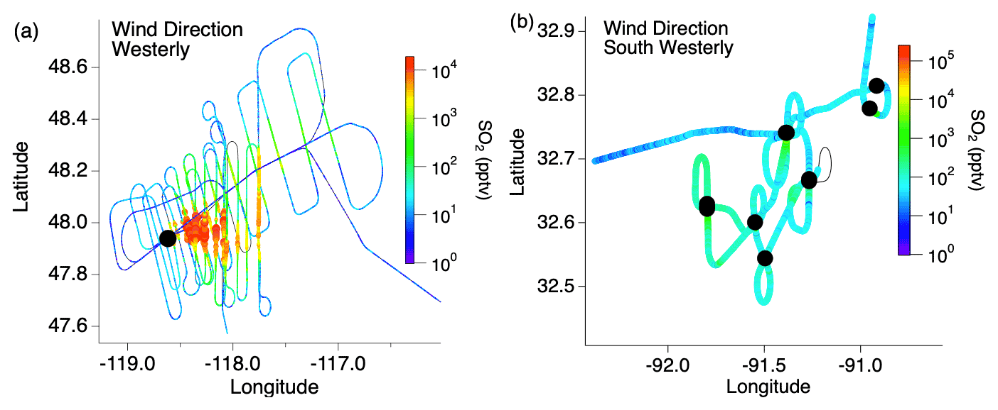
Figure 1 Typical flight path through (a) wildfire and (b) agricultural fire smoke plumes with the color and size of the markers indicating the SO₂ mixing ratio and the black markers indicating the fire locations.

In situ measurements of SO₂ were performed using laser-induced fluorescence (LIF SO₂) in which SO₂ was excited at 216.9 nm by a custom-built fiber laser system with the red-shifted fluorescence detected between 240 and 400 nm. An intercomparison performed between the LIF SO₂ and Caltech chemical ionization mass spectrometer (CIMS) during FIREX-AQ showed good agreement between the two measurement techniques (Rickly et al., 2021). The accuracy of the LIF SO₂ measurements is ±9 % +2 pptv, primarily dictated by uncertainty in the calibration standard concentration and spectroscopic background.

Sulfate measurements were performed by a suite of in situ instruments: an Aerodyne high-resolution time-of-flight aerosol mass spectrometer (AMS) (DeCarlo et al., 2006; Canagaratna et al., 2007) with a sampling rate of 1–5 Hz, the online soluble acidic gases and aerosol mist chamber (SAGA-MC) coupled with an ion chromatograph (IC) (Scheuer et al., 2003; Dibb et al., 2002) with a sampling interval of 75 s, and a SAGA filter collector with subsequent offline IC analysis (Dibb et al., 1999, 2000), with typical sampling intervals of 3 min in the large fires. Both SAGA-MC and AMS sample submicron particles, while the SAGA filter collects both submicron and supermicron particles up to 4.1 µm with 50 % transmission (McNaughton et al., 2007; van Donkelaar et al., 2008; Guo et al., 2021). The AMS instrument allows for the speciation of submicron non-refractory particulate mass and the direct separation of inorganic and organic species having the same nominal mass-to-charge ratio (DeCarlo et al., 2006; Canagaratna et al., 2007). Both inorganic sulfate and organic sulfate fragment similarly in the AMS, mostly to H_xSO${}_y^{+}$ ions without carbon. For AMS total nitrate, for which the fragmentation pattern is similar (Farmer et al., 2010), techniques for rapid assignment of organic nitrate based on its fragmentation pattern have been successfully developed (Fry et al., 2013; Day et al., 2022). While there are some differences in fragmentation between organic and inorganic sulfur that have been used in some cases to separate organic from inorganic sulfate (Chen et al., 2022; Dovrou et al., 2019), the sulfate fragmentation pattern is overall much more variable compared to nitrate, and hence such approaches will work only in very specific instances (Schueneman et al., 2021). In this work, we found the ion fragmentation method to produce reasonable results based on the consistency with the results using positive matrix factorization (PMF, Paatero et al., 1994; Ulbrich et al., 2009) and the measurements of submicron sulfate aerosol from SAGA-MC, which quantifies only inorganic sulfate. The correlation between the AMS inorganic sulfate and SAGA-MC sulfate shows overall good agreement (Fig. S8), which adds confidence to the AMS apportionment. However, as discussed in Sect. 4.2.2, for certain types of organosulfur compounds, hydrolysis in the liquid phase after capture into the instrument and before analysis might lead to SAGA-MC detecting these as well, and hence the SAGA-MC sulfate measurements are likely more uncertain under FIREX-AQ conditions based on the default accuracy estimates for this instrument (Dibb et al., 2002; Scheuer et al., 2003).

Both IC (SAGA) instruments detect HMS as S(IV) and the signal interfered with sulfite and bisulfite. There is no unambiguous detection of HMS specifically in either the IC or the AMS.

In situ CO concentrations were measured via wavelength modulation spectroscopy (Sachse et al., 1991), with an uncertainty of 2 %–7 % over the dynamic range of the measurements. In situ CO₂ concentrations were measured with non-dispersive infrared spectrometry using a modified commercial spectrometer (model 7000, LI-COR) similar to Vay et al. (2009), with uncertainties varying between 0.25 ppm and 2 % of the measurements (whichever is larger) over the range of the measurements.

2.2 Emission factor calculation

Emission factors (EFs) are defined as the mass of compound X relative to the mass of fuel burned; however, this can be substituted with the mass balance method, which approximates the fuel mass by the sum of emitted carbon (Andreae, 2019). In accordance, the emission factors for SO₂ and sulfate were calculated as the enhancement ratio of each compound relative to the enhancement ratio of total carbon emitted per fire in units of grams per kilogram (g kg⁻¹) (Eq. 1). Because CO and CO₂ comprise approximately 95 % of total carbon emissions, the summation of these values was used to represent total carbon.

$$\begin{array}{}\text{(1)}& \mathrm{EF}\left(\mathrm{X}\right)={\displaystyle \frac{\mathrm{X}}{\mathrm{CO}+{\mathrm{CO}}_{\mathrm{2}}}}\cdot {\displaystyle \frac{{\mathrm{MM}}_{\mathrm{X}}}{{\mathrm{MM}}_{\mathrm{C}}}}\cdot F_{\mathrm{C}}\cdot \mathrm{1000}\end{array}$$

The orthogonal distance regression slope of compound X to total carbon $\left(\frac{\mathrm{X}}{\mathrm{CO}+{\mathrm{CO}}_{\mathrm{2}}}\right)$ was determined for each transect through the smoke plume with a smoke age <1 h to limit the influence of chemical processing due to atmospheric aging. Only emission ratio values with R²>0.5 were included in the EF analysis. It is shown in Sect. 3.3 and 3.7 that no significant aging of SO₂ occurs within this length of time. In addition, only measurements ≥25 % enhanced from the background were used, which allowed the background mixing ratios to be neglected. MM_X and MM_C represent the molar mass of compound X and the summation of CO and CO₂, respectively. The approximated value of 45 % is used to represent the carbon fraction (F_C) of the fuel emitted during these biomass burning events as outlined by Susott et al. (1996) and allows for a more direct comparison to the compilation of EF data prepared by Andreae (2019).

2.3 Modified combustion efficiency

The modified combustion efficiency (MCE) is a metric for combustion stage. The MCE is defined as the enhancement of CO₂ from the background in relation to the summation of the enhanced CO and CO₂ mixing ratios (Eq. 2). Traditionally, MCE > 0.9 is indicative of the flaming stage and an MCE < 0.9 is representative of the smoldering stage (Ferek et al., 1998; Sinha et al., 2003; Zhang et al., 2018). In reality, smoke sampled from large wildfires likely reflects a combination of variable fractions of flaming and smoldering combustion.

$$\begin{array}{}\text{(2)}& \mathrm{MCE}={\displaystyle \frac{{\mathrm{CO}}_{\mathrm{2}}}{\mathrm{CO}+{\mathrm{CO}}_{\mathrm{2}}}}\end{array}$$

2.4 Box model

The Framework for 0-D Atmospheric Modeling (F0AM, Wolfe et al., 2016) was used to evaluate the evolution of SO₂ downwind of the fire location (Wolfe et al., 2016). Within F0AM, the Master Chemical Mechanism (MCM) version 3.3.1 was used to describe the evolution and chemistry of the gas-phase SO₂ and oxidant species. An additional mechanism describing the conversion of SO₂ to sulfate was implemented to address aerosol oxidation processes of sulfur compounds based on an establishment of equilibrium of the S(IV) compounds and oxidant species with relation to pH (Tang et al., 2014; D'Ambro et al., 2016; Seinfeld and Pandis, 2006). A complete list of the aqueous-phase reactions and measurements used for model input is included in Tables S1 and S2 and the mechanism code is provided in Supplement Sect. 2.

The model was implemented to investigate the chemistry that occurred during the Williams Flats fire, which started 2 August 2019 by lightning ignition of timber and/or slash fuels in Keller, WA. Two separate flight days, 3 and 7 August, were modeled here using measurements acquired by the DC-8 in which two passes of lawnmower patterns were completed. These flights were analyzed by applying a Lagrangian model approach. The measurements were corrected for dilution by normalizing to CO (Müller et al., 2016) as follows:

$$\begin{array}{}\text{(3)}& {\mathrm{\Delta }}_{\mathrm{dil}}\mathrm{X}={\displaystyle \frac{(\mathrm{X}-{\mathrm{X}}_{\mathrm{b}})}{(\mathrm{CO}-{\mathrm{CO}}_{\mathrm{b}})}}\cdot {\mathrm{CO}}_i,\end{array}$$

in which $\frac{\mathrm{X}}{\mathrm{CO}}$ represents the ratio of compound X at each transect with respect to CO, X_b and CO_b are the background concentrations, and CO_i represents the carbon monoxide mixing ratio at the source of the fire determined from the extrapolation of the transect average CO values. This extrapolation method was also applied to the dilution-normalized mixing ratios in order to initialize the model back to the fire source (t=0). The model was constrained to these initial concentrations, then allowed to run freely through the remainder of the flight time. The dilution rate was determined by matching the modeled CO to the measured CO decay using a Gaussian fit. However, CO_i, used to determine the dilution-normalized mixing ratio values, was based on the extrapolated CO initial value based on all transect CO values (core and edge).

Measurements were acquired through aircraft smoke plume penetration, which provided pseudo-Lagrangian observations by not entirely following the same air parcel. Comparison to a Lagrangian simulation is challenging because the aircraft measured different parts of the plume (core vs. edge) and at different emission times. As a result, an exponential fit applied to the SO₂ and sulfate dilution-normalized mixing ratios against plume age is used to represent the measurement trend for comparison to the model results. While the model is not expected to precisely reproduce the measurements based on plume age due to variations in altitude between transects and subsequently varied pressures and temperatures, it does allow for the comparison of the overall trends of SO₂ and sulfate downwind of the source using averaged meteorological constraints.

Uptake of SO₂ and the oxidant species (O₃, NO₂, H₂O₂, and HCHO) to aerosol was represented within the model mechanism as a first-order loss (Seinfeld and Pandis, 2006):

$$\begin{array}{}\text{(4)}& k_{\mathrm{het}}=\mathrm{0.25}\cdot \mathit{\gamma }\cdot c\cdot \mathit{\nu },\end{array}$$

where γ represents the uptake coefficient, c is the mean molecular speed of SO₂, and ν is the aerosol surface area based on average dry particle size distributions measured by a laser aerosol spectrometer (model 3340). To account for the gas-phase diffusion limitation, γ was calculated by the following equation:

$$\begin{array}{}\text{(5)}& \mathit{\gamma }={\displaystyle \frac{\mathrm{1}}{\mathit{\alpha }}}+{{\displaystyle \frac{\mathrm{0.75}+\mathrm{0.286}Kn}{Kn\cdot (Kn+\mathrm{1})}}}^{-\mathrm{1}},\end{array}$$

where α represents the mass accommodation coefficient and Kn is the Knudsen number. Mass accommodation and gas diffusion coefficients used for deriving Kn and γ are listed in Table S3.

To represent equilibrium partitioning between the gas and aqueous phases, rates of condensation and evaporation were applied as described by D'Ambro et al. (2016):

$$\begin{array}{}\text{(6)}& {\displaystyle }{k}_{\mathrm{cond}}=k_{\mathrm{het}},\text{(7)}& {\displaystyle }{k}_{\mathrm{evap}}={\displaystyle \frac{k_{\mathrm{het}}}{H\cdot \mathrm{LWC}}},\end{array}$$

where H represents the Henry's law constant of the species being adsorbed and LWC is the liquid water content of the cloud or aerosol. The dry particle size (not ambient particle size) is incorporated into k_het through Eq. (4). This k_het value is then applied to Eq. (7) as a ratio to the LWC and ability of uptake (H), allowing for calculation of the gas–particle equilibrium. Therefore, as the particle size increases, greater condensation is able to occur, but this also allows for increased evaporation. However, with an increase in LWC and H, less evaporation will be expected. Using this method of uptake and evaporation does not allow equilibrium of all processes to be assumed as is done in the ISORROPIA calculations. Because S(IV) production is pH-dependent, individual equilibrium constants in relation to the H⁺ produced by each reaction are required as an additional factor in the k_evap denominator as described by Seinfeld and Pandis (2006). As a result, the model accurately reproduces the S(IV) pH dependence (Fig. S1a) in which HSO${}_{\mathrm{3}}^{-}$ is the dominant form in the pH range of 2–7 and SO${}_{\mathrm{3}}^{\mathrm{2}-}$ becomes the dominant form at pH > 7. Table S1 lists all aqueous-phase reactions.

The rate of S(IV) oxidation exhibits a pH dependence based on the available oxidant species (Table S1) (Cheng et al., 2016). Using our model and the initial conditions from Guo et al. (2017b), we reproduced pH-dependent oxidation rates very similar to those shown in that study. However, initializing the model with the higher concentrations observed during FIREX-AQ increases the rates of oxidation as shown in Fig. S1b. This results in S(IV) oxidation being dominated by reaction with hydrogen peroxide at pH values < 5, which is within the range that aerosol sulfate production most commonly occurs in the US. For pH values approaching 5, there may be some competition amongst H₂O₂, O₃, and HCHO depending on the oxidant concentrations. As pH values increase above 5, O₃, NO₂, and HCHO become the dominant oxidants with H₂O₂ and NO₂ oxidation declining rapidly. Although the reaction of HCHO with S(IV) results in HMS production rather than inorganic sulfate, it has been included here to demonstrate its impact on S(IV) oxidation. HCHO adduct formation follows a very similar trend as O₃ oxidation, becoming a major S(IV) reactant at higher pH. Further discussion of the HMS reactions listed in Table S1 can be found in the Supplement.

In this study, aerosol LWC and pH were determined via ISORROPIA-II thermodynamic modeling (Fountoukis and Nenes, 2007) in forward mode based on the AMS-measured aerosol composition (SO₄, NO₃, NH₄, Cl) and collocated gas-phase measurements of NH₃ and HNO₃ from proton transfer reaction–mass spectrometry (PTR-MS) and CIMS, respectively. NH₃–NH₄ is the most important species pair for constraining pH because it was not completely in either the gas or particle phase in the fire plumes or the background air mass. To improve the accuracy in thermodynamic modeling predictions, we removed the outliers when the predicted particle-phase fraction of the NH₃–NH₄ partitioning is off by > 40 % compared to the observation (4.6 % of the data). The gas–particle partitioning is reproduced with ISORROPIA-II, with the regression slopes of predicted NH₃, NH₄, and NO₃ close to 1 compared to the observations and highly correlated (slopes: 0.949, 1.116, and 1.002; r²: 0.991, 0.96, and 0.99996, respectively). This also supports the assumption of equilibrium, as the characteristic time for fine particle water equilibrium is very short (<1 s) (Pilinis et al., 1989) and ranges from 20 min or less (Dassios and Pandis, 1999; Cruz et al., 2000; Fountoukis et al., 2009; Guo et al., 2018) up to 10 h for semivolatile components, NH₃, HNO₃, and HCl (Meng and Seinfeld, 1996; Fridlind and Jacobson, 2000; Shingler et al., 2016). The uncertainty in particle pH is estimated to be within 0.5–1 units based on the sensitivity of pH to NH₃–NH₄ partitioning and varies from point to point depending on the model reproduction of the partitioning (Guo et al., 2017a). Because these calculations are based on the inorganic aerosol concentrations, the LWC could potentially be up to several times greater due to the dominant organic portion in the fire plumes despite the lower hygroscopicity compared to the inorganics (Kreidenweis et al., 2008; Guo et al., 2015; Brock et al., 2016). The mixing state of inorganic and organic for the particles in the early-phase plumes remains to be investigated but is likely to be phase-separated given the low oxidation state of the organics (Sullivan et al., 2020). The current modeling can be interpreted as assuming a phase separation of inorganic vs. organics, with the chemistry studied occurring only in the inorganic-dominated phase and its associated water, with no kinetic limitations due to potential core–shell or micelle-like structures present in the particles. Propagating the uncertainties of AMS inorganics (34 %, 2σ) (Bahreini et al., 2009)) and DC-8 total water measurement (3 % based on the observed RH) gives an LWC uncertainty of 39 % (Guo et al., 2015). Due to the dominant organic fraction of sulfate signals in the fire plumes investigated in this study, additional bias and uncertainty derive from using the total AMS SO₄ signals and zero non-volatile cations (e.g., not accounting for the potential contribution of soluble ions from ash, Adachi et al., 2022) in estimating LWC and pH. This is of particular concern when the uncertainties are larger than the estimated free acidity based on ion balance, as often happens near the neutralization point. The potential bias is estimated to be $-\mathrm{0.96}\pm \mathrm{0.95}$ units for pH (i.e., biased low).

Most importantly, the modeling work presented in this study assumes an ideal solution. Given the relatively high ionic strength conditions observed for the 3 August (89.5 ± 19.3 M) and 7 August (83.2 ± 25.3 M) flights due to the overall rather low RH, this can potentially lead to high deviations in the actual gas uptake coefficients, aqueous-phase rate coefficients, and, to a lesser extent, pH (calculation of which does account for ionic strength but is fairly under-constrained under these conditions).

3 Results and discussion

3.1 Emission factors

The elemental sulfur EFs calculated for FIREX-AQ are comparable to previous reports. As described in Sect. 2.33, flaming and smoldering delineation was determined by an MCE value of 0.9. For consistency with other FIREX-AQ reports, the fuel types listed remain as subcategories but are combined for comparison to the comprehensive biomass burning fuel types listed by Andreae (2019). The FIREX-AQ agriculture category comprises measurements of residual burns of rice, corn, and soybean fields. Across the fuel types measured during FIREX-AQ (Fig. 2), we find that SO₂ is consistently larger than sulfate when calculated as EFs of elemental sulfur, indicating that, at most, a minor fraction of SO₂ (20 %–25 %) is converted to sulfate within 1 h downwind (or emitted directly as primary sulfate). Where data are not reported, this is due to either missing data or a low correlation with total carbon (R² < 0.5). The total sulfur EFs agree reasonably well with those reported by Andreae et al. (1988), which were measured in the Amazon basin, in the range of 0.24–0.66 g S kg⁻¹ C.

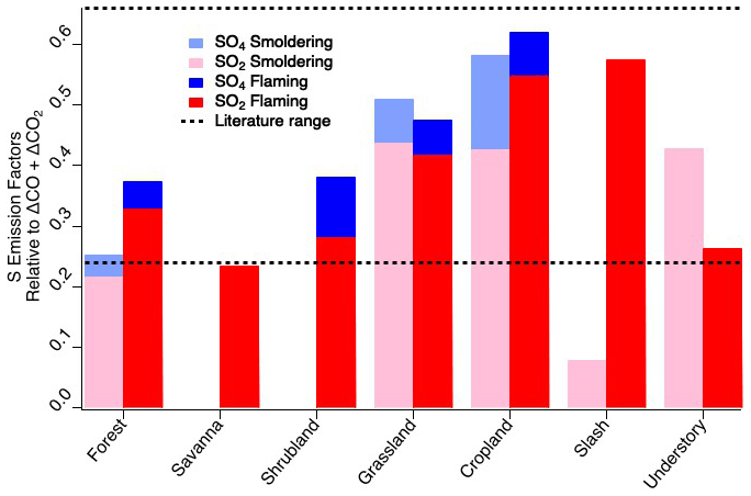
Figure 2 Elemental sulfur emission factors of SO₂ and sulfate by fuel type and combustion stage within 1 h downwind compared to literature values of total sulfur emission factors.

No trend with MCE is observed for SO₂ EFs when separated by the various fuel types for smoldering and flaming conditions above MCE 0.85 for SO₂ and sulfate (Fig. 3). It has previously been suggested that EFs can be calculated based on MCE for use by the global climate modeling community. There have been conflicting opinions around this suggestion, with some species showing relevant correlations, while other species do not (Yokelson et al., 1996; Burling et al., 2011; Akagi et al., 2013). Considering all the EFs for SO₂, sulfate, and the ratio of SO₂ to sulfate under 1 h shows that, individually, SO₂ and sulfate do not show strong correlations with MCE (Fig. 3). However, the ratio of the two produces a stronger correlation, suggesting there may be a relationship in which more sulfate may be produced during smoldering combustion and more SO₂ emitted during flaming combustion. One possibility is that the smoke plumes from smoldering fires are more conducive to rapid conversion of SO₂ to sulfate such that the ratio of SO₂ and sulfate has significantly decreased by the time it is sampled. This could be due to a number of factors, including higher aerosol EF, which, depending on the aerosol composition, could allow for more rapid aqueous-phase oxidation. It is also possible that more primary sulfate is emitted from those plumes.

Figure 3 Scatter plots of EFs for SO₂ (a), sulfate (b), and the ratio of SO₂ to sulfate (c) (within 1 h downwind of each fire source) vs. MCE based on combined fuel types.

Averaging the flaming and smoldering EFs produces an overall SO₂ EF of 0.73 ± 0.43 g SO₂ kg⁻¹ C. This is within the combined variability of the Andreae (2019) compilation of flaming and smoldering EFs of 0.62 ± 0.75 g kg⁻¹ C, which excludes peat and laboratory fires. Separating the SO₂ EFs by combustion stage results in a flaming stage value of 0.80 ± 0.46 g kg⁻¹ C (0.62 ± 0.61 g kg⁻¹ C from Andreae, 2019) and a smoldering stage value of 0.62 ± 0.36 g kg⁻¹ C (0.61 ± 0.27 g kg⁻¹ C from Andreae, 2019). While the FIREX-AQ flaming stage value is considerably higher than the Andreae (2019) compilation, the two are within the combined variability of the observations. However, this higher average EF for the flaming stage FIREX-AQ measurements is strongly influenced by the large number of measurements of longleaf pine and agricultural fuels, which had high EF values.

Looking more closely at the different fuel types in comparison to the categories compiled by Andreae (2019), we see good agreement within the combined variability (Table 1 and Fig. 4). While the fuel types are categorized differently in this study, many still fit the characteristics of the categories listed in the compilation report, allowing for comparison. Of the FIREX-AQ categories that allow for comparison with Andreae (2019), all EF data available are for the flaming stage.

Table 1 Comparison of the flaming stage SO₂ EFs (g kg⁻¹ C) by fuel type as measured during FIREX-AQ (left) to the compiled values reported in Andreae (2019) (right).

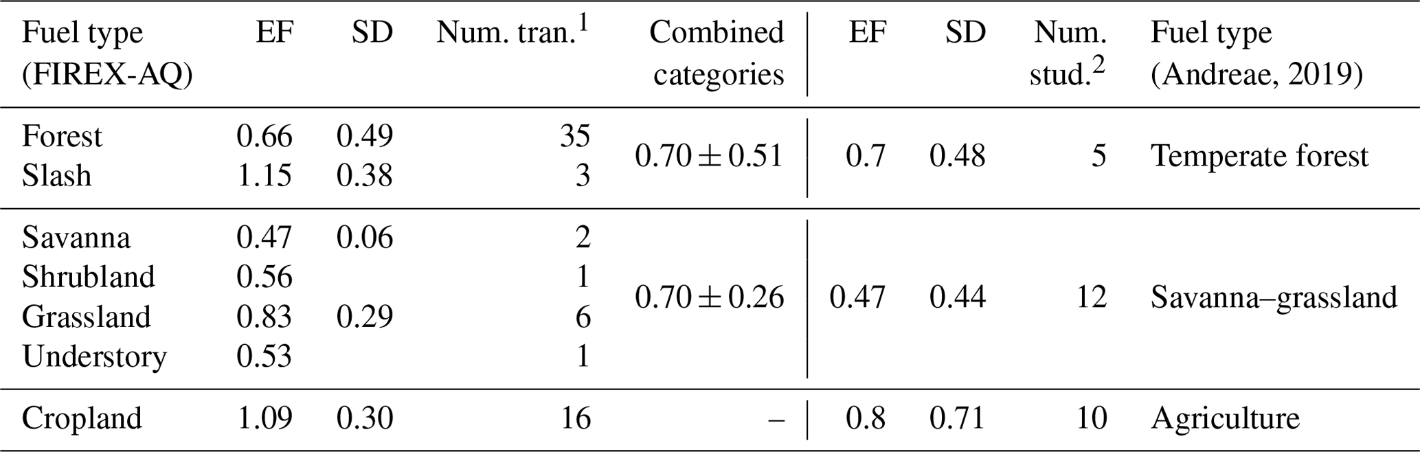
¹ “Num. tran.” indicates the number of transects measured within 1 h downwind of the fire source measured during FIREX-AQ.
² “Num. stud.” indicates the number of studies included in the Andreae (2019) compilation.

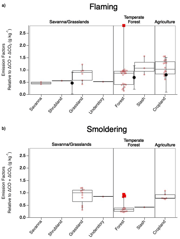
Figure 4 Comparison of SO₂ EF values observed during flaming (a) and smoldering (b) combustion across fuel types sampled during FIREX-AQ. The box upper edge represents the 75th percentile and the lower edge the 25th percentile with the median shown by the middle line. The whiskers represent the minimum and maximum observed values with the open circles representing each observation and the solid red circle representing a potential outlier. The large solid black circles with error bars depicting 1 standard deviation in (a) show corresponding average Andreae (2019) values.

The generally strong agreement between FIREX-AQ EFs and those in published inventories lends confidence to the quality of EFs underlying model emissions. Agricultural burns exhibit the highest EFs. This was reported by Andreae (2019) as 0.80 ± 0.71 g kg⁻¹ C in the flaming stage, similar to 1.1 ± 0.30 g kg⁻¹ C reported here. The temperate forest category, comprised here of forest and slash, produces a combined EF of 0.70 ± 0.51 g kg⁻¹ C, which is in excellent agreement with the Andreae (2019) value of 0.7 ± 0.48 g kg⁻¹ C. Combining savanna, shrubland, grassland, and understory into the savanna–grassland category produces the largest difference in which the FIREX-AQ value of these combined fuels is 0.70 ± 0.26 g kg⁻¹ C, whereas Andreae (2019) reported a value of 0.47 ± 0.44 g kg⁻¹ C; however, these values fit within the standard deviation.

The categories measured during FIREX-AQ that do not overlap with the Andreae (2019) compilation reflect smoldering conditions. For the most part, the majority of the smoldering stage SO₂ EFs exhibit lower values than the flaming stage by approximately 21 %–63 % (Fig. 4). The two FIREX-AQ categories (grassland and understory) which show smoldering SO₂ EFs to be larger than the flaming stage suggest the need for additional measurements to build statistical confidence.

3.2 Emission factor variability

The variability observed amongst the different fuel types may partly reflect variability in surface S content stemming from wet and dry deposition. Although this source of sulfur has significantly decreased in the US over the last 2 decades, the highest emission factors during FIREX-AQ were observed within the regions of the US that typically experience the largest sulfur deposition rates as reported by the National Atmospheric Deposition Program (2022) (Fig. 5).

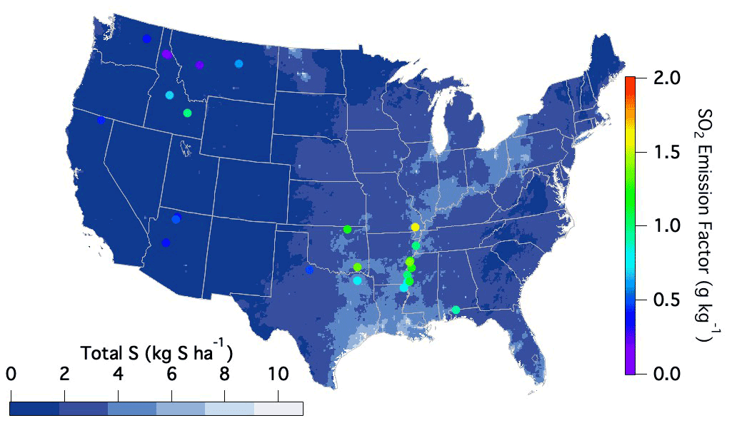
Figure 5 National Atmospheric Deposition Program (2022) reported sulfur deposition rates (https://nadp.slh.wisc.edu/committees/tdep/#tdep-maps, last access: 1 May 2021) compared to SO₂ EFs (closed circles) by geographical location as measured during FIREX-AQ for all fuel types.

Sulfur-containing fertilizers may also enhance S content in smoke. Sulfur aids plant uptake of nitrogen, and decreasing sulfur deposition over the last 2 decades has led to increased use of sulfur additives in fertilizers (Hinckley et al., 2020). Hinckley et al. (2020) report this sulfur application to range from around 20–300 kg S ha⁻¹ yr⁻¹, which occurs in the form of inorganic sulfate or elemental sulfur (Solberg et al., 2011). Given that the average yield of corn within the US is 168 bushels per acre, a sulfur application of 20 kg S ha⁻¹ yr⁻¹ would result in 12 g S kg⁻¹ C in its composition. Assuming 10 % of this added sulfur remains after harvest and runoff and is present in the residual material that is burned, the remaining 1.2 g S kg⁻¹ could in part explain the enhanced emission factors in those regions (US Department of Agriculture, 2020). Therefore, the observed variability in emission factors throughout the US may in part be explained by the sulfur availability to the plants and soils from either deposition or fertilizer use, resulting in larger emission factors from certain locations when burned.

4 Chemical evolution of sulfur

After emission, SO₂ oxidizes to sulfate via both gas- and condensed-phase processes. Discrepancies reported by previous studies of modeled sulfate compared to measurements suggest that the conversion chemistry of SO₂ to sulfate is not fully understood. In this section, we combine FIREX-AQ observations with a detailed chemical box model to evaluate the chemical mechanisms of SO₂ to sulfate conversion.

4.1 Temperature dependence of sulfate production efficiency

The balance of gas- and particle-phase sulfur between SO₂ and sulfate exhibits a marked temperature dependence amongst the cumulative flights while remaining generally constant during individual flights (Fig. 6). The fewer observations at temperatures below 265 K are the result of the range of aircraft altitude sampled during this study. However, the decreasing trend shown by the numerous measurements between 265 and 283 K supports the suggestion of lower SO₂ concentrations compared to sulfate at the lower temperatures. Sulfate is > 90 % of the sum at temperatures below 265 K, while above 285 K SO₂ and sulfate are equally balanced, which is likely due to the quasi-second-order process of heterogeneous oxidation in a plume (Freiberg, 1978). The noisy but overall positive trend between 265 and 283 K suggests rapid chemistry after emission. Conversion of SO₂ to sulfate generally increases with decreasing temperature due to increased aerosol water content as well as SO₂ and oxidant solubility, but the rapid change observed in this temperature regime also requires aqueous-phase sulfur oxidation (Pattantyus et al., 2018).

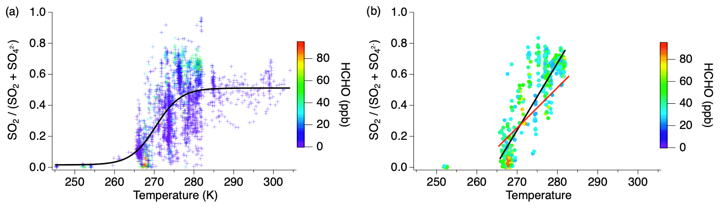
Figure 6 Fractional sulfur conversion as a function of temperature (a) including all smoke ages with a sigmoid fit and (b) only measurements with HCHO > 25 ppb with the black line indicating the linear fit through the data at all ages between 265–283 K and the red line indicating the linear fit through the measurements within 1 h of emission in the same temperature regime.

The majority of sulfur oxidation occurs in the aqueous phase. As observed during the 3 August flight, calculation of the contribution of OH to the decrease in SO₂ by applying an OH concentration of 2×10⁶ cm⁻³ (Liao et al., 2021) produces a negligible SO₂ decay compared to the dilution-normalized mixing ratio of SO₂ (Fig. S2). Similar behavior is expected for other flights due to similar conditions of limited photolysis near the center of the smoke plume.

Recent studies have suggested HCHO to be an important aqueous-phase oxidant at reduced temperatures (Moch et al., 2018; Song et al., 2021). However, HCHO is also an indicator of smoke age, with mixing ratios typically being largest nearest to the fire source (Liao et al., 2021). Considering measurements acquired when the HCHO mixing ratio is high (>25 ppb) and implicitly filtering out aged smoke, the slope of the SO₂ to total sulfate ratio over the 265–283 K temperature regime (0.04) shows a stronger correlation with temperature (R²=0.74) (Fig. 6b, black line). Further limiting the effect of chemical aging by analyzing only those measurements within 1 h of the fire source, the conversion of SO₂ to sulfate is observed to be approximately 65 % slower (Fig. 6b, red line) in the 265–283 K temperature range. This is consistent with heterogeneous chemistry in that aging occurs more rapidly at higher temperatures. While sulfate measurements within 1 h of the fire source could be due to primary emission, this is expected to be a small fraction compared to SO₂, as shown in Fig. 2, and primary emission would not exhibit the temperature dependence observed here.

Other sulfate species contribute to sulfur conversion during this temperature regime. There were several periods identified during these flights in which organosulfur species were recognized to be a significant fraction of the AMS sulfate measurement. These measurements only occurred within the temperature range 270–285 K. When organosulfur was present in plume transects within 1 h downwind of the fire source, the SO₂ to total S ratio decreased with decreasing temperature 23 % faster than in transects of fresh plumes when organosulfur was not present.

These findings emphasize the importance of temperature in combination with smoke age and organosulfur production for the conversion of SO₂ to sulfate and are further investigated in Sect. 4.2.1.

4.2 Model results

4.2.1 Williams Flats 3 August 2019 flight

Select time series relating to the conversion of SO₂ to sulfate for the 3 August 2019 flight are shown in Fig. S3. Altitude and temperature were constant at around 3 km and 280 K for both passes of about 10 transects each. Actinic fluxes trended downward for the second pass as dusk approached. Thermodynamic modeling suggests an average pH value of 5.3 (range of −2 to 8) over the length of the plume transects, but a possible increase in LWC by a factor of 2–3 during the second pass with an average of $\mathrm{2}\times {\mathrm{10}}^{-\mathrm{6}}$ g sm⁻³. Because the conditions of this flight are relatively consistent between passes, the measurements of both passes are combined for comparison to the model with pH and LWC held constant. Modeling results of this flight with the inclusion of all known gas- and aqueous-phase S(IV) pathways (Table S1) are shown in Fig. 7 with a conservatively assumed 30 % uncertainty. This range encompasses the uncertainties associated with the mechanism of aqueous-phase uptake and chemical rate constants occurring at the specified LWC and pH.

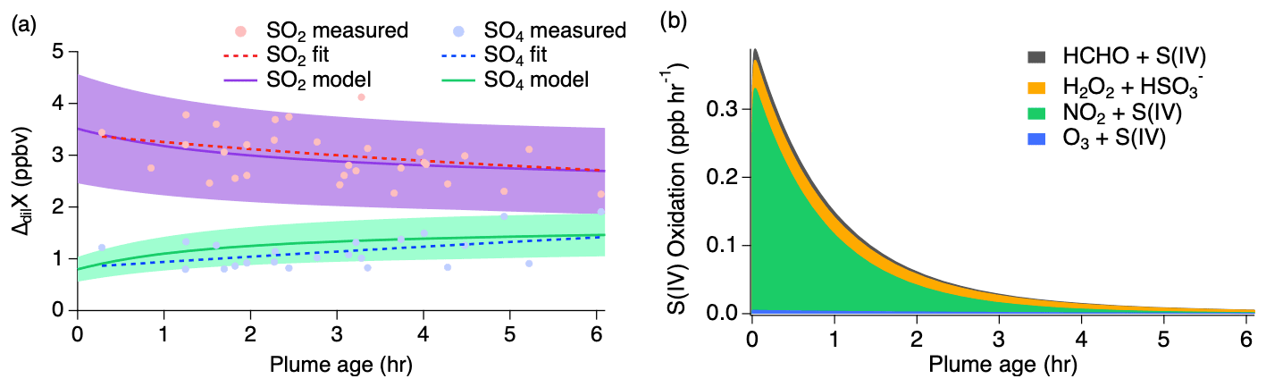
Figure 7 (a) Dilution-corrected (Δ_dilX) measurements of 3 August 2019 shown by the markers and measurement fits shown by the dashed lines compared to the SO₂ and sulfate model results represented by the solid lines, with shading denoting an estimated 30 % model uncertainty. The sulfate (SO₄) measurements represent total sulfate which potentially includes organosulfur. (b) Stacked modeled S(IV) oxidation rates leading to sulfate and HMS production.

The model reproduces the general measurement trend of the 3 August flight for both SO₂ and sulfate (Fig. 7a). Model results for NO, NO₂, $\mathrm{NO}/{\mathrm{NO}}_{\mathrm{2}}$, O₃, HCHO, and H₂O₂ are compared to the measurements for each model in Fig. S4, showing good agreement for the 3 August flight. In accordance with the sulfate measurements, the modeled sulfate represents the sum of sulfate and HMS (the latter representing OS). A small, yet important, change is observed for the SO₂ and sulfate measurements with SO₂ decreasing by a linear slope of 0.15 ppb h⁻¹ and sulfate increasing by a linear slope of 0.26 ppb h⁻¹. The decrease in the S(IV) reactions (Fig. 7b) further demonstrates this. The largest increase in these reactions is observed within the first 15 min, but the decrease in these reactions over the remaining 6 h indicates a slowing of this conversion. Under the conditions of this flight, the model indicates that aqueous-phase oxidation by NO₂ and H₂O₂ is the dominant pathway leading to inorganic sulfate formation with little S(IV) reaction by HCHO and O₃ (Fig. 7b). This is in contrast to what has been previously expected of aerosol S(IV) oxidation, which has been thought to be dominated by ozone oxidation. However, the higher NO₂ oxidation rate constant with increased pH reported by Liu and Abbatt (2021) for nonideal solutions increases the significance of this reaction.

4.2.2 Williams Flats 7 August 2019 flight

The 7 August 2019 flight shows distinct differences between the two passes (Fig. S5); therefore, the flight has been differentiated into the first pass (first full set of transects) and second pass (second full set of transects). It is also during this flight that the largest OS contribution has been reported for the AMS measurements during the FIREX-AQ wildfire flights.

The first pass was measured around 4 km and 276 K with an estimated dilution factor of approximately $\mathrm{8}\times {\mathrm{10}}^{-\mathrm{5}}$ s⁻¹ and limited cloud presence. A pH of around 7.2 was estimated for this flight with an aerosol LWC of approximately $\mathrm{1}\times {\mathrm{10}}^{-\mathrm{7}}$ g sm⁻³. Both NO₂ and CO decrease at similar rates, while HCHO remains relatively stable around 40 ppb and O₃ shows a decrease compared to the air outside the plume for the first six transects (Fig. S6). SO₂ and sulfate are fairly similar, with a few instances of sulfate surpassing SO₂ in addition to a moderate fraction of OS observed during this pass.

The increased altitude of the second pass is associated with an 8 K decrease in temperature relative to the first pass. The dilution factor for this pass was determined to be slower at around $\mathrm{3}\times {\mathrm{10}}^{-\mathrm{5}}$ s⁻¹. The difference in these dilution factors could be due to measuring at different altitudes or the result of a sampling artifact due to measuring in different sections of the plume; however, there is not enough information available to determine the exact cause. NO₂ appears to decrease more slowly in comparison to CO, which remains relatively constant after the plume has moved away from the clouds. In addition, ozone, which shows the same trend as O_x, appears to be consumed more quickly in transects in which clouds were observed, suggesting rapid uptake within the clouds, in addition to the fast reaction with NO producing the additional NO₂. This additional NO₂ in combination with limited photochemistry as a result of decreasing actinic flux (Fig. S7) due to approaching dusk conditions slows the decreasing NO₂ trend observed during this pass. Furthermore, ISORROPIA calculations indicate a 10-fold increase in aerosol LWC in the presence of clouds compared to the first pass. This is likely due to the decrease in temperature (268 K) and larger relative humidity. The presence of clouds decreases downwind concurrently with a decrease in relative humidity, but aerosol LWC remains high. Lastly, this pass shows that SO₂ is nearly depleted in the center of the plume (Fig. S5), while sulfate increases substantially with a rather significant fraction of OS being observed (Fig. S8).

Due to these distinct differences between passes, each pass was modeled separately with the OS contribution reported independently from the sulfate measurements and model results. The modeled oxidation compounds (Fig. S4) show generally good agreement with the measurements for these passes; however, some discrepancies are observed due to measuring different parts of the plume. Results of the first pass are shown in Fig. 8 and the second pass shown in Fig. 9; both show good agreement between the model and measurements with ozone and NO₂ as the largest contributors to sulfate production during this flight. However, the majority of modeled S(IV)reaction occurs through the HCHO pathway rapidly producing HMS.

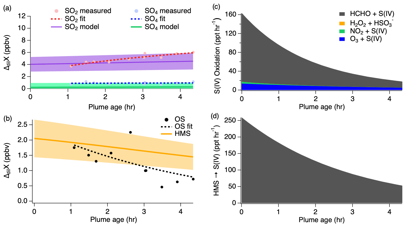
Figure 8 First pass dilution-corrected (Δ_dilX) measurements shown by the markers and measurement fits shown by the dashed lines compared to the model results represented by the solid lines, with shading denoting an estimated 30 % model uncertainty for SO₂ and sulfate (a) as well as OS (b). Stacked modeled S(IV) oxidation rates (c) leading to sulfate and HMS production. HMS reverse reaction rate (d) reproducing S(IV).

The first pass shows SO₂ increasing downwind, which is unexpected because SO₂ is considered to be a primary emission which typically decreases downwind as it is removed through oxidation. In addition, the measurements show a large OS mixing ratio following the first hour after emission before gradually decreasing downwind. This suggests that OS is either directly emitted from the fire source or very rapidly produced.

Clouds and large LWC were present throughout the majority of the second pass measurements (Figs. S5 and S6), significantly shifting the chemistry from that of the first pass. Figure 9 shows that modeled SO₂ is quickly taken up into the aqueous phase under higher LWC conditions $(\mathrm{6}\times {\mathrm{10}}^{-\mathrm{5}}$ g sm⁻³) and pH (7.2) with approximately 1.5 ppb going directly into sulfate production and the remaining 3 ppb of the initial SO₂ concentration being converted into HMS. These reaction processes occur promptly after emission, but they rapidly slow once all of the available initial SO₂ is depleted within the first 1–2 min. The exponential trends of the sulfate and OS measurements agree with the model results to within approximately 40 %.

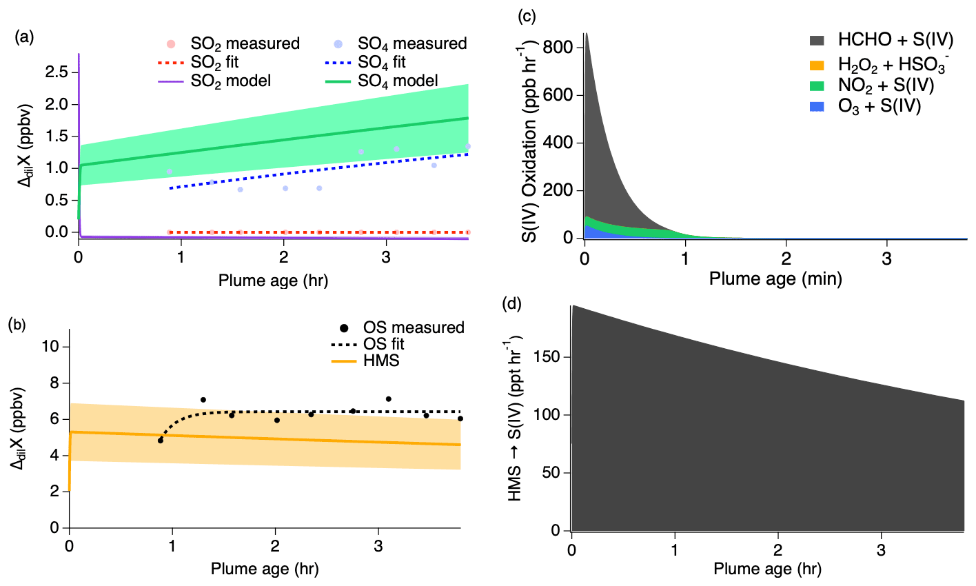
Figure 9 Second pass dilution-corrected (Δ_dilX) measurements shown by the markers and measurement fits shown by the dashed lines compared to the model results represented by the solid lines, with shading denoting an estimated 30 % model uncertainty for SO₂ and sulfate (a) as well as OS (b). Stacked modeled S(IV) oxidation rates (c) leading to sulfate and HMS production. HMS reverse reaction rate (d) reproducing S(IV).

Comparing the 3 and 7 August flights, the main differences leading to the different S(IV) reaction pathways are the pH and HCHO mixing ratios. Average pH on the 3 August flight was 5.3, whereas the 7 August flight experienced neutral conditions with a pH around 7.2. The initial HCHO mixing ratio was estimated to be 30 ppb for the 3 August flight and 50 ppb for the 7 August flight. While liquid water content plays a significant role in affecting the HMS reversal rate, each of these flights remained within the wet aerosol characterization with a calculated LWC of $\mathrm{2}\times {\mathrm{10}}^{-\mathrm{6}}$ g sm⁻³ for the 3 August flight and $\mathrm{66}\times {\mathrm{10}}^{-\mathrm{6}}$ g sm⁻³ (4 km) and $\mathrm{66}\times {\mathrm{10}}^{-\mathrm{5}}$ g sm⁻³ (5 km) for the 7 August flight. The total S observed for these flights in terms of SO₂ and sulfate shows values of 2–10 ppb on average above the background; however, in the presence of organosulfates, this total S can increase to up to 15 ppb on average above the background.

The importance of HMS as an S(IV) reservoir and its conversion into sulfate or into gas-phase SO₂ largely depends on the varying conditions of LWC. Under neutralized conditions (7.2), the model reproduces the observed trends of all three compounds under these wet aerosol conditions. As discussed further in Sect. 4.2.3, the higher pH of this flight increases the rate of HMS reversal back into S(IV) by a factor of 6. Because of the low LWC of the first pass, heterogeneous uptake is limited and causes the rates of S(IV) reaction to significantly decrease. S(IV) evaporation then enhances gas-phase SO₂ in transported smoke, consistent with similar rates of HMS decay and SO₂ growth. As a result, very little sulfate is produced during this pass at a rate of approximately 4 ppt h⁻¹ primarily due to S(IV) oxidation by ozone. However, the higher LWC conditions of the second pass allow S to remain in the aqueous phase. The small increase in sulfate of approximately 500 ppt over the course of the flight can be explained by a small fraction of HMS on the order of 120–190 ppt h⁻¹, which undergoes a reverse reaction decomposing back into S(IV) before being oxidized to produce sulfate (Fig. 9d).

The SAGA-MC instrument detects HMS as S(IV), which cannot be separated from HSO${}_{\mathrm{3}}^{-}$ and SO${}_{\mathrm{3}}^{\mathrm{22}-}$ and is therefore subject to interference from high concentrations of gas-phase SO₂. However, the S(IV) from the SAGA-MC is comparable to the SAGA filter samples, which are unaffected by ambient SO₂, and hence suggests that a large fraction of the S(IV) in the SAGA-MC was present in the aerosol and that the contribution of the SO₂ artifact to the S(IV) signal is small. This observation further suggests that most of the S(IV) was present in submicron particles, as supermicron particles are not quantified by the SAGA-MC (Guo et al., 2021). As shown in Fig. S9, SAGA-MC sulfate measurements show concentrations similar to the AMS inorganic sulfate measurements during both passes. The AMS total sulfate is slightly larger than the SAGA-MC sulfate in the first pass but considerably larger during the second pass. The SAGA-MC S(IV) (reported as SO₃) was similar to AMS SO_4,org on the first pass but did not increase with AMS SO_4,org during the second pass, suggesting that HMS may have constituted the majority of the organosulfur concentrations measured during the first pass but that an additional unknown organosulfur was much more abundant than HMS during the second pass. Therefore, it appears that the modeled HMS exceeds measurements on the second pass.

There are two potential explanations for the good agreement between the observed organosulfur concentration from the second pass and the modeled HMS. It is possible that during the very rapid uptake of SO₂ into the aqueous phase, (1) additional organosulfur species may be produced or (2) the additional organosulfur species are the result of further reactions of HMS, suggesting that the model is correctly reproducing the HMS formation chemistry but indicating that the model aqueous-phase chemistry is incomplete. Both of these potential explanations require the measured organosulfur species to behave similarly to HMS in their rates of formation and termination in order to explain the good agreement between the modeled HMS and measured organosulfur concentrations. In addition, these explanations would require the organosulfur species to not be identified as S(IV) in ion chromatography measurements. It is a potential possibility with the large mixing ratios of HCHO and H₂O₂ observed in these fire plumes that the chemistry of hydroxymethyl hydroperoxide as a result of HCHO and H₂O₂ reaction could be influencing the organosulfur production and should be considered in future studies (Dovrou et al., 2022). While the modeling allows significant insight into the identity and formation mechanisms of aerosol sulfur, there is not enough evidence available from these measurements to conclusively explain all of the AMS and SAGA-MC sulfur observations.

4.2.3 Model HMS sensitivity analysis

We performed a model sensitivity analysis to investigate the relevance of organosulfur behavior under the conditions of the HMS rates of production and termination in different environments by varying the model LWC (10⁻⁶–1 g sm⁻³), pH (1–8), temperature (260–280 K), and HCHO (10–90 ppb) individually while holding the other parameters constant at the 3 August flight conditions (T=280 K, pH = 5.3, and LWC = $\mathrm{2}\times {\mathrm{10}}^{-\mathrm{4}}$ g sm⁻³) due to the more simplified chemistry occurring during this flight.

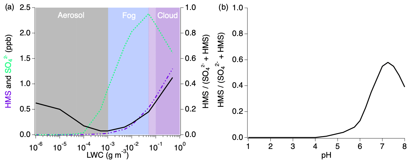
Figure 10 Sensitivity analysis of HMS formation under individually varied LWC and pH conditions. The black line in each figure represents the ratio of the modeled HMS mixing ratio to the sum of the modeled inorganic sulfate and HMS.

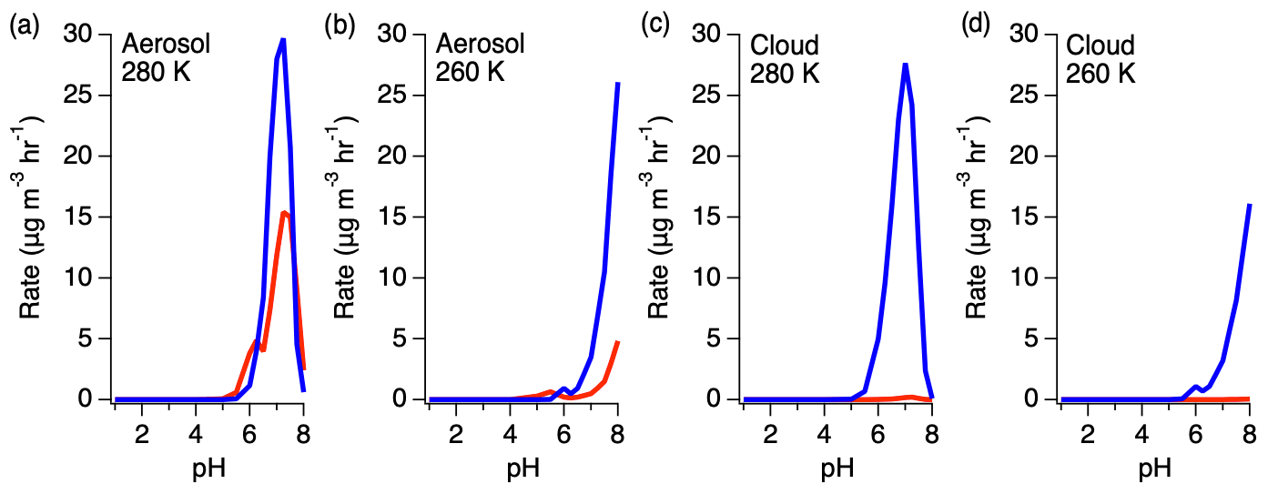
Figure 11 Rates of HMS production (red) and reversal (blue) under aerosol and cloud conditions at 280 and 260 K.

Variations in LWC (Fig. 10a) show that aerosols with less LWC produce minimal amounts of sulfate and HMS but that HMS makes up between 5 % and 45 % of the combined concentrations. The HMS fraction shows the largest contribution as LWC increases into the cloud regime at which point sulfate production begins to decrease with a rapid increase in HMS. While the typical LWC range estimated for these fires is 10⁻⁷–10⁻² g sm⁻³, this indicates that the chemistry of the smoke will change substantially with cloud interactions. LWC is shown to be an important variable in the ratio of the formation of HMS to sulfate; however, this ratio trend is indicative of conditions at pH 5.3 and will vary under differing pH conditions.

The pH dependence of the ratio of $\mathrm{HMS}/({\mathrm{SO}}_{\mathrm{4}}+\mathrm{HMS})$ is shown in Fig. 10b in which HMS formation is more active as the acidity decreases. At acidic pH values representative of typical tropospheric aerosol (Nault et al., 2021), a negligible amount of HMS contributes to the combined concentrations. Above pH 4, the HMS contribution begins to increase, followed by a more rapid increase after pH 6. The maximum HMS contribution is reached around pH 7.3 before rapidly decreasing at higher values.

The ratio of HMS production and reverse reactions varies with pH, with the reverse reaction becoming more substantial at higher pH (Fig. 11). Under aerosol LWC conditions, the rate of the HMS reverse reaction is up to 3 times larger than the rate of HMS production. As LWC increases into the cloud regime, the rate of the HMS reverse reaction increases further to approximately 2 orders of magnitude larger than HMS production around pH 7. However, a reduction in temperature shifts this dependence to higher pH, decreasing the rate of HMS reversal at the same pH.

While temperature and HCHO concentration are key factors controlling HMS production, these factors alone under low LWC and pH result in minimal HMS (Fig. S10). HMS production increases with decreasing temperature; however, under the conditions of the 3 August flight, HMS only reaches a maximum value of 5 ppt at 260 K, which is approximately 5 % of the modeled sulfate. Similarly, a minimal amount of HMS is produced with varied HCHO, but the ratio of HMS to the sum of HMS and sulfate increases linearly with HCHO at a rate of 1.5 ppt ppb⁻¹ HCHO.

The conditions that most largely affect HMS are LWC and pH. Due to the significance of LWC to HMS production and reversal, it is likely that aqueous aerosols, fog, cloud droplets, and possibly ice crystals will be most impactful on HMS production. Because the rainwater pH of areas such as the western US and eastern China can reach much less acidic pH levels due to increased ammonia emissions, it is likely that these areas will be more susceptible to HMS production (Keresztesi et al., 2020; Qu and Han, 2021). Together, these conditions indicate that highly polluted areas which experience higher pH and greater LWC will likely be influenced by this chemistry. Therefore, the production of HMS should be an important consideration for air quality in areas such as agricultural regions which experience enhanced emissions of ammonia, likely increasing the pH, as well as geographical locations which may promote fog formation. This would include areas such as Beijing, the Uinta Basin, and Bakersfield, CA, which have observed severe haze formation and have the potential to be affected by HMS.

5 Conclusions

SO₂ plays an important role in sulfate aerosol formation and thus air quality and climate forcing. Therefore, understanding the sources and evolution of SO₂ emissions in a changing climate is essential. The emission factors determined from the FIREX-AQ mission under flaming conditions show good agreement with the compilation reported by Andreae (2019). This provides confidence for the same categories under smoldering conditions for which there are no reported measurements from previous studies. No distinct correlation is observed for SO₂ emission factors based on MCE; however, it remains unclear if fire MCE influences the ratio of SO₂ and sulfate emission factors. With biomass burning events increasing worldwide, this study suggests that the resulting SO₂ emission factors will be more dependent on geographical location and land use and less dependent on combustion phase and fuel type. Areas that incur more sulfur deposition from coal burning or application through fertilizer use will likely produce larger SO₂ emission factors.

Modeling with inclusion of the HCHO reaction chemistry (producing HMS) shows good agreement with the measurements. However, the differentiation of HMS from sulfate through the SAGA-MC measurements indicates that HMS can be overpredicted. While HMS is potentially directly emitted from the fire source, a large organosulfur concentration is observed that has not yet been identified. Because the modeled HMS is similar to the measured organosulfur fraction, it is expected that the additional organosulfur species likely exhibit similar rates of production and termination as HMS. The importance of the HMS, or similar species, reverse reaction is also made apparent by the ability to act as an S(IV) reservoir. This allows these species to produce sulfate or SO₂ further downwind depending on the LWC and pH.

Environments that experience high LWC and pH are expected to be the most influenced by this chemistry. This includes regions that experience higher ammonia emissions and are geographically or meteorologically subject to greater cloud or fog formation. As a result, this chemistry should be considered when assessing severe haze events as a result of either biomass burning or industrial pollution.