Water vapour and ozone in the upper troposphere–lower stratosphere: global climatologies from three Canadian limb-viewing instruments

This study presents upper troposphere–lower stratosphere (UTLS) water vapour and ozone climatologies generated from 14 years (June 2004 to May 2018) of measurements made by three Canadian limb-viewing satellite instruments: the Atmospheric Chemistry Experiment Fourier Transform Spectrometer (ACE-FTS), the Measurement of Aerosol Extinction in the Stratosphere and Troposphere Retrieved by Occultation (MAESTRO), and the Optical Spectrograph and InfraRed Imaging System (OSIRIS; ozone only). This selection of instruments was chosen to explore the capability of these Canadian instruments in representing the UTLS and to enable analysis of the impact of different measurement sampling patterns. The water vapour and ozone climatologies have been constructed using tropopause-relative potential temperature and equivalent-latitude coordinates in an effort to best represent the distribution of these two gases in the UTLS, which is characterized by a high degree of dynamic and geophysical variability. Zonal-mean multiyear-mean climatologies are provided with 5^∘ equivalent latitude and 10 K potential temperature spacing and have been constructed on a monthly, seasonal (3-month), and yearly basis. These climatologies are examined in-depth for two 3-month periods, December–January–February and June–July–August, and are compared to reference climatologies constructed from the Canadian Middle Atmosphere Model 39-year specified dynamics (CMAM39-SD) run, subsampled to the times and locations of the satellite measurements, in order to evaluate the consistency of water vapour and ozone between the datasets. Specifically, this method of using a subsampled model addresses the impact of each instrument's measuring pattern and allows for the quantification of the influence of different measurement patterns on multiyear climatologies. This in turn permits a more consistent evaluation of the distributions of these two gas species, as assessed through the differences between the model and measurement climatologies. For water vapour, the average absolute relative difference between CMAM39-SD and ACE-FTS differed between the two versions of ACE-FTS by less than 8 %, while the MAESTRO climatologies were found to differ by 15 %–41 % from ACE-FTS, depending on the version of ACE-FTS and the season. When considering the ozone climatologies, those constructed from the two ACE-FTS versions agreed to within 2 % overall, and the OSIRIS ozone climatologies agreed with these to within 10 %. The MAESTRO ozone climatologies differ from those from ACE-FTS and OSIRIS by 30 %–35 % and 25 %, respectively, albeit with regions of better agreement within the UTLS. These findings indicate that this set of Canadian limb sounders yields generally similar water vapour and ozone distributions in the UTLS, with some exceptions for MAESTRO depending on the season and gas species.

1 Introduction

Long-term observational and model-derived climatologies are widely used to represent the zonal-mean state of atmospheric constituents for a specific period as a function of altitude and geolocation coordinates. These climatologies provide information on the atmospheric environment and permit investigations into the distribution of trace gases and the patterns resulting from circulation and transport processes (e.g., Randel et al., 1998; Jones et al., 2012; Koo et al., 2017). Additional uses of climatologies include evaluating systematic differences between model or observational datasets (e.g., Eckstein et al., 2017; Kolonjari et al., 2018), evaluating trends (e.g., Deeter et al., 2018), and acting as a priori information for the retrieval of trace gas profiles from measurements (e.g., Vigouroux et al., 2008; Sofieva et al., 2014). In recent years, there has been a push to expand the database of climatologies focused on one of the most challenging regions of the atmosphere to study, the upper troposphere–lower stratosphere (UTLS), in order to better constrain the role the UTLS plays in climate processes through the detailed characterization of the constituents of the region (SPARC-CCMVal, 2010; SPARC, 2017; Kunkel et al., 2018).

The UTLS is a crucial region of chemical, radiative, and dynamical activity in the atmosphere, spanning from approximately 300 to 30 hPa (e.g., Holton et al., 1995; Gettelman et al., 2011). The tropopause, a dynamic barrier to transport that acts to separate the vertical transport regimes of the troposphere and stratosphere, strongly influences the chemical structure of the UTLS (Holton et al., 1995; Hoor et al., 2002; Pan et al., 2004). Stratosphere–troposphere exchange via localized processes, such as tropopause folds and components of the Brewer–Dobson circulation, permits some chemical transport between the underlying and overlying regions, but overall the tropopause greatly restricts trace gas transport, giving rise to strong gradients in the horizontal and vertical (e.g., Holton et al., 1995; Roelofs and Lelieveld, 1997; Hoor et al., 2002; Pan et al., 2004; Hoor et al., 2010). Many of these mixing processes are variable in nature, leading to rapidly changing small-scale gas features that further impact the trace gas distributions around the UTLS (Holton et al., 1995; Roelofs and Lelieveld, 1997; Hoor et al., 2002; Pan et al., 2004; Hoor et al., 2010). The frequency of these localized mixing processes around the tropopause, along with the inherent variability of the tropopause and the large vertical and horizontal trace gas gradients at the tropopause, leads to the high degree of variability characteristic of the UTLS (Holton et al., 1995; Pan et al., 2004).

As a result of radiative effects arising from the thermal structure of the UTLS, knowledge of the distribution of trace gases within this region is critical in the development of an accurate understanding of climate forcing. Atmospheric temperatures are at a local minimum in the UTLS, maximizing the thermal contrast of the upwelling infrared radiation absorbed as compared to that emitted, which in turn maximizes the influence of gases that absorb in the infrared on the atmospheric forcing of surface temperature (Forster and Shine, 1997, 2002; Gettelman et al., 2011; Riese et al., 2012). This holds for water vapour and ozone, which this effect makes two of the most important greenhouse gases (Lacis et al., 1990; Forster and Shine, 1997; Solomon et al., 2010). Outside of their role as greenhouse gases, these two species collectively influence the chemical composition of the UTLS by providing ice surfaces for heterogeneous chemical reactions (water vapour; Brasseur and Solomon, 2005), producing hydroxyl radicals that rapidly react with other gases (Brasseur and Solomon, 2005), and by absorbing ultraviolet and infrared light to moderate the energy balance of the UTLS (Lacis et al., 1990; Brasseur and Solomon, 2005). Water vapour is primarily concentrated near the surface, with a strong negative gradient extending upwards to the tropopause following the lapse rate, while ozone is mainly concentrated in the stratosphere, with a gradient extending polewards from its maximum concentration in the tropical middle stratosphere where the majority of ozone production occurs. The limited stratospheric water vapour arises mainly from upward transport at the Equator, though these air parcels are largely dehydrated when passing through the cold tropical tropopause region, with the oxidation of methane, largely in the middle and upper stratosphere, serving as a smaller secondary source (Holton et al., 1995; Brasseur and Solomon, 2005; Lossow et al., 2017). In the free troposphere, ozone is enhanced by stratosphere–troposphere processes that move air parcels rich in ozone down into the troposphere, including the seasonally varying Brewer–Dobson circulation (Roelofs and Lelieveld, 1997; Lelieveld and Dentener, 2000; Pan et al., 2004).

Despite the large impact the UTLS has on climate, it remains one of the least well characterized regions of the atmosphere because of the challenging measurement conditions posed by the region. Included in this are the relatively low chemical concentrations of many of the trace gas constituents compared to their concentrations elsewhere in the troposphere or stratosphere, the presence of clouds that can inhibit remote observations over widely employed measurement frequencies, and the frequent localized mixing processes around the tropopause, which, along with the inherent variability of the tropopause itself, lead to the high degree of variability characteristic of the UTLS (Holton et al., 1995; Pan et al., 2004). Many UTLS-focused studies use aircraft and balloon-borne instruments, including ozonesondes and frost-point hygrometers, to make highly vertically resolved measurements of water vapour and ozone (e.g., Kunz et al., 2011; Hurst et al., 2011; Zahn et al., 2014; Eckstein et al., 2017). The detail provided by these measurements facilitates process studies; however analysis of temporal and spatial variations is restricted as measurements are often regionally focused, performed as part of discontinuous measurement campaigns, or both (Kunz et al., 2008; Zahn et al., 2014). Detailed analysis of UTLS composition, including long-term trends in trace gases, requires decadal global observational datasets, which satellite instruments are capable of providing (e.g., Hegglin et al., 2010, 2021). However, satellite instruments can still encounter difficulties making measurements in the UTLS because of, for example, the coarse vertical sensitivity of nadir-viewing instruments, which can prevent vertical UTLS features from being well resolved, or because of the long path lengths of limb-viewing instruments, which can smear out finer structures in UTLS gas distributions. Chemistry–climate models can aid investigations into climate forcers, such as greenhouse gases, by providing detailed simulations of chemical and transport processes; however, these must be evaluated against measurements to ensure their veracity (e.g., Pendlebury et al., 2015; Kolonjari et al., 2018).

The need for well-characterized trace gas climatologies that can serve towards the parallel goals of analyzing gas distributions and trends and of evaluating model datasets is emphasized in the reports produced as a part of the Stratosphere-troposphere Processes And their Role in Climate (SPARC) Chemistry-Climate Model Validation Activity (SPARC-CCMVal, 2010) and the SPARC Data Initiative (SPARC, 2017) projects. Key recommendations for future work from this latter activity highlighted the need to study the UTLS in greater detail to address outstanding questions concerning the behaviour of trace gases (SPARC, 2017). Specifically, the climatologies analyzed in the SPARC Data Initiative included the UTLS, but emphasis was on the stratosphere as a whole and only a small subset of associated activities (e.g., Neu et al., 2014) focused on the UTLS in particular. To fully characterize the differences between instruments in the UTLS, this report stressed the need for climatologies to be constructed in ways that best minimize the effects of geophysical variability on the diagnostics compared (SPARC, 2017).

In recent years, many major activities and individual studies have considered water vapour and ozone as measured by a variety of satellite instruments. Included in this list of activities is the SPARC Water Vapour Assessment II (WAVAS II), the SPARC Long-term Ozone Trends and Uncertainties in the Stratosphere (LOTUS), the Stratospheric Water and Ozone Satellite Homogenized (SWOOSH) climate data record, and the European Space Agency's Water Vapour Climate Change Initiative (WV_cci) and Ozone Climate Change Initiative (Ozone_cci), with some projects employing well over a dozen instrument datasets (e.g., Davis et al., 2016; Lossow et al., 2019; SPARC/IO3C/GAW, 2019; Hegglin et al., 2021; Read et al., 2022). While many of these activities have a UTLS component, the majority of recent studies are not focused on climatologies, or in cases where they are, these are not made with a focus on the UTLS, such as the recent update to the SPARC Data Initiative (Hegglin et al., 2021). One of the driving principles of the ongoing SPARC Observed Composition Trends And Variability in the Upper Troposphere and Lower Stratosphere (OCTAV-UTLS) activity is to address the need for UTLS-focused climatologies, produced with an aim to minimize the effects of geophysical variability by accounting for geophysical conditions (Kunkel et al., 2018). Additionally, this activity aims to address the influence of disparate sampling patterns in this region to maximize the use of available datasets. As reported by Toohey and von Clarmann (2013) and Millán et al. (2016), nonuniform sampling by instruments due to their measurement patterns can introduce significant systematic errors when comparing datasets, which is not accounted for in many comparison studies of climatologies. Toohey et al. (2013), as part of the SPARC Data Initiative, found that sampling biases can lead to differences around the UTLS in excess of 10 % between water vapour measurement climatologies and in excess of 20 % between ozone climatologies, emphasizing the need to better constrain this error in future climatology comparisons.

With this in mind, the aim of this study is to produce, analyze, and compare zonal-mean multiyear-mean water vapour and ozone climatologies that utilize data from three Canadian limb-viewing satellite instruments, the Atmospheric Chemistry Experiment Fourier Transform Spectrometer (ACE-FTS), the Measurement of Aerosol Extinction in the Stratosphere and Troposphere Retrieved by Occultation (MAESTRO), and the Optical Spectrograph and InfraRed Imaging System (OSIRIS; ozone only), in support of the OCTAV-UTLS activity. All three instruments measure down into the UTLS with high vertical resolution, have long data records, and provide global coverage over the course of the year, making them good fits to study this highly variable region (Bernath et al., 2005; McElroy et al., 2007; Haley et al., 2004, respectively). While data from these instruments have been used in previous climatology studies (e.g., Neu et al., 2014; SPARC, 2017; Hegglin et al., 2021), the climatologies produced here use tropopause-referenced vertical coordinates, which can reduce differences in climatologies arising from different sampling of geophysical variability by parcelling the data based on the processes which drive some of this variability, thereby ensuring only data driven by similar geophysical processes are assessed or compared (e.g., Pan et al., 2004; Hoor et al., 2004; Hegglin et al., 2008; Manney et al., 2011). Specifically, tropopause-referenced potential temperature is employed because of its ability to account for the role of the tropopause as a transport barrier, which enables it to represent the large trace gas gradients that arise around the tropopause, leading to improved partitioning of data (e.g., Pan et al., 2004; Manney et al., 2011). The meridional coordinate used in these climatologies is potential-vorticity-derived equivalent latitude, which can group air masses based on dynamical conditions, thereby reducing the effect of sporadic meridional transport in the UTLS on comparisons (e.g., Hoor et al., 2004; Hegglin et al., 2006). However, this coordinate possesses limitations, such as in representing tropospheric transport processes, as shown in Manney et al. (2011) and Pan et al. (2012). In spite of these limitations, through the combination of these coordinates the inherent variability in the UTLS can be constrained better in the resulting climatologies.

The climatologies presented here cover the 14-year period between 1 June 2004 and 31 May 2018 and are intended to both provide a well-characterized representation of water vapour and ozone, as measured by the three instruments involved in this study, and provide a source of data for future work including intercomparison studies and model evaluation. To characterize the differences between the datasets, the Canadian Middle Atmosphere Model 39-year specified dynamics (CMAM39-SD) model output dataset is used as a consistent comparison reference for this analysis, though it should be noted that this does not imply that the model output serves as a standard outside of this. Adapting the methods of Kolonjari et al. (2018), the model is sampled at the times and locations of the instrument measurements in order to generate subsampled model climatologies of ozone and water vapour, which permits the sampling-related differences between the datasets to be explored free from the influence of any retrieval biases between the instruments. In addition to the multiyear-mean climatologies, these equivalent-latitude zonal-mean climatologies are also produced on a monthly basis for the same 14-year period, detailed examination of which is outside of the scope of this study.

The rest of the paper is organized as follows; Sect. 2 addresses the satellite and model simulation datasets used, along with the means by which the tropopause height and equivalent latitude are determined for the datasets. Section 3 addresses the method used to generate water vapour and ozone climatologies, as well as the approach taken to comparing these climatologies using a set of subsampled model climatologies. Sections 4 and 5 explore the resulting climatologies of water vapour and ozone, along with an intercomparison between the climatologies for each gas generated from each dataset. Finally, a summary is presented in Sect. 6.

2 Datasets

This section outlines the datasets used in this study. Section 2.1 through 2.3 cover the satellite instruments used, one of which contributes two data versions to this study, while Sect. 2.4 addresses the reanalysis products that provide auxiliary data about atmospheric conditions for these measurement products. Section 2.5 describes the model output employed in this study.

2.1 ACE-FTS

The Canadian satellite SCISAT-1 was launched into a circular low-Earth orbit (650 km altitude, 74^∘ inclination) on 12 August 2003 (Bernath et al., 2005). A primary objective of the Atmospheric Chemistry Experiment (ACE) mission aboard SCISAT-1 is to study chemical and dynamical processes impacting ozone distributions in the upper troposphere and stratosphere, using the solar occultation measurement technique (Bernath et al., 2005). Scientific operations of the ACE instruments commenced in February 2004 and are ongoing.

A Fourier transform spectrometer, ACE-FTS, makes measurements covering the spectral range 750–4400 cm⁻¹ with 0.02 cm⁻¹ spectral resolution (Bernath et al., 2005; Boone et al., 2005, 2013, 2020). Operating in a limb-viewing geometry, ACE-FTS records absorption spectra twice per orbit, corresponding to sunrise and sunset occultations as seen by the instrument. Measurements are made at tangent heights spanning from the cloud tops to 150 km, with vertical spacing between 1.5 and 6 km and a vertical field of view of 3–4 km (Bernath et al., 2005). In the UTLS, the vertical resolution of ACE-FTS combined with oversampling throughout the region leads to an effective resolution of about 1 km, making it ideal for studying gases in this region (Hegglin et al., 2008; Kolonjari et al., 2018). Under typical conditions, up to 15 sunrise and 15 sunset measurements can be made per day. Over the course of the year the latitudinal coverage of ACE-FTS spans from 85^∘ N to 85^∘ S, with a focus on the polar regions; however, due to the orbital inclination of SCISAT-1, it takes approximately 3 months to cover this range (Bernath, 2017).

Vertical profile information about temperature, pressure, and concentration as the volume mixing ratio (VMR) for several dozen trace gas species comes from inversions of the solar occultation measurements made by ACE-FTS. The retrieval process is described fully in Boone et al. (2005, 2013, 2020), but in brief it begins with a CO₂ analysis through which pressure and temperature profiles are established. Using these temperature and pressure profiles, a global Levenberg–Marquardt nonlinear least-squares-fitting algorithm is applied to the measured spectra to yield VMR profiles for the desired gas species. As part of the retrieval, the profiles are made available on a uniform 1 km grid (Boone et al., 2005, 2013).

In this work both version 3.6 (v3.6) and version 4.2 (v4.2) profiles of water vapour and ozone are used. While v3.6 (and its predecessor version 3.5, which uses an identical algorithm but in a different computational environment) ozone and water vapour profiles have been extensively validated and studied (e.g., Sheese et al., 2017; Bognar et al., 2019; Lossow et al., 2019), v4.2 is still undergoing validation (e.g., Sheese et al., 2022). As described in Boone et al. (2020), a key difference between these versions is that v4.2 retrievals use a CO₂ input for the temperature and pressure retrievals that explicitly accounts for seasonal and latitudinal variations and has an improved temporal variation compared to the v3.6 CO₂ input, as well as consideration of the age of air in the stratospheric distribution of CO₂. Additionally, CO₂ is retrieved below 18 km in v4.2, necessitating that temperature and pressure information below this altitude is obtained from operational outputs from a global weather assimilation and forecasting system. A consequence of retrieving CO₂ is that in the v4.2 retrieval, the instrument pointing information is determined through analysis of the N₂ continuum, as opposed to analysis of CO₂ lines as done in the v3.6 retrieval (Boone et al., 2020). A set of quality control flags have been developed for the ACE-FTS v3.6 and v4.2 products (Sheese et al., 2015). These are applied to the ACE-FTS data used in this work to filter extreme outliers from the data, with all flagged outlier measurements removed as recommended in Sheese et al. (2015). This method was found to reject 3.0 % of v3.6 H₂O, 1.8 % of v3.6 O₃, 1.6 % of v4.2 H₂O, and 1.0 % of v4.2 O₃ profiles used in this study. ACE-FTS data products have been used previously for a variety of applications, including for climatology development (e.g., Jones et al., 2012; Koo et al., 2017; SPARC, 2017; Hegglin et al., 2021), trend analysis (e.g., Fernando et al., 2020), and model studies and validation (e.g., Pendlebury et al., 2015; Kolonjari et al., 2018).

Recent work by Sheese et al. (2022) found that one of the key impacts on the trace gas products from the change from ACE-FTS v3.6 to v4.2 is that the newer version corrects a systematic drift in the former. Specifically, in comparing coincident measurements of ozone from ACE-FTS v3.6 and v4.2 against an ensemble of five different instruments, the ACE-FTS v3.6 product was found to experience a significant drift of −1.0 ± 0.4 % per decade between 20 and 35 km, whereas no drift of any significance was detected in the ACE-FTS v4.2 product (Sheese et al., 2022). The observed drift in the ACE-FTS v3.6 ozone product arose from inaccurate CO₂ modelling, which would likewise impact the v3.6 water vapour product (Sheese et al., 2022). Below 21 km, Sheese et al. (2022) found that neither ACE-FTS version displayed a significant drift.

Global coincident measurement comparisons by Sheese et al. (2017) showed that ACE-FTS v3.5 water vapour concentrations are about 5 % lower than those measured by the Michelson Interferometer for Passive Atmospheric Sounding (MIPAS) and 5 %–20 % lower than the Aura Microwave Limb Sounder (Aura-MLS) measurements in the lower stratosphere. In the upper troposphere, the bias with MIPAS is between −5 % and +15 % and Aura-MLS yields larger concentrations of water vapour, in particular near the lower bound of sensitivity where the difference exceeds 50 %. Further comparisons of the ACE-FTS v3.5 water vapour dataset by Lossow et al. (2019) against an ensemble of coincident global satellite instruments indicated that ACE-FTS v3.5 water vapour in the lower stratosphere is about 3 %–8 % drier than other measurements, while in the upper troposphere ACE-FTS is drier by approximately 10 %–40 %. However, comparisons with the Stratospheric Aerosol and Gas Experiment III instrument on the International Space Station (SAGE III/ISS) by Davis et al. (2021) showed a wet bias for ACE-FTS v3.6 exceeding 20 % in the upper troposphere and at about 5 % in the lower stratosphere. Comparisons of coincident measurements made by ACE-FTS v3.6 against the Polar Environment Atmospheric Research Laboratory Fourier transform infrared spectrometer (PEARL FTIR) in the Canadian high Arctic indicated that ACE-FTS has a wet bias compared to this instrument of 7 %–10 % in the UTLS. Further comparisons against in situ radiosondes contrasted this by yielding a slight dry bias in ACE-FTS v3.6, of about 0 %–9 %, in the upper troposphere and a slight wet bias, of less than 2 %, in the lower stratosphere (Weaver et al., 2019).

Sheese et al. (2017) also examined ACE-FTS v3.5 ozone and found it to be within ±5 % of both Aura-MLS and MIPAS in the lower stratosphere, while in the upper troposphere these differences reached as high as 30 % for MIPAS and 40 % for Aura-MLS, with ACE-FTS biased low at these lower altitudes. McCormick et al. (2020) compared the v3.6 ozone profiles to SAGE III/ISS and found similar agreement, to within ±5 %, as did Sheese et al. (2017) over the lower stratosphere. Bognar et al. (2019) found ACE-FTS v3.6 ozone over the high Arctic to be about 5 % larger in the upper troposphere and 5 % smaller in the lower stratosphere than OSIRIS and 5 %–10 % larger than MAESTRO throughout the UTLS. In addition to their work in evaluating the drift in the ACE-FTS products, Sheese et al. (2022) determined that ACE-FTS v3.6 ozone is biased high by 3 %–5 % between 15 and 25 km, while the ACE-FTS v4.2 ozone bias ranged from −1 % to +5 % over this same altitude range, as determined from a weighted comparison to MAESTRO, OSIRIS, the Sounding of the Atmosphere using Broadband Emission Radiometry (SABER) instrument on the NASA TIMED satellite, Aura-MLS, and the Odin Sub-Millimetre Radiometer (Odin-SMR).

Climatologies have also been compared as done in Hegglin et al. (2021), the update to the SPARC (2017), which compared water vapour and ozone climatologies to multi-instrument mean climatologies. They found ACE-FTS v3.6 has a high bias for ozone in the upper troposphere by about 10 %–20 % that transitions to a roughly 3 %–5 % high bias in the lower stratosphere, with an exception for the southern polar region, which is biased low by about 20 %. ACE-FTS v3.6 water vapour was found to be biased high over the upper troposphere by 20 %–50 % and generally biased low in the lower stratosphere, by 0 %–10 %, with an exception for the southern polar region where differences can approach 50 % (Hegglin et al., 2021). These findings agree with recent work for ACE-FTS water vapour (Lossow et al., 2019), as do the lower stratospheric differences for ozone (Sheese et al., 2022), but some disagreement is noted between climatological and profile comparisons in the upper troposphere for ozone. Part of this discrepancy is the result of nonuniform temporal sampling of ACE-FTS, which can lead to larger biases when comparing climatologies than when comparing coincident profiles between datasets due to variations in trace gas distributions over time. This holds for climatological comparisons made with other measurement datasets and spurs the use of subsampled model comparisons in this work.

2.2 ACE-MAESTRO

The second instrument aboard SCISAT-1 is MAESTRO, a dual spectrograph designed to measure between 285 and 1030 nm, with the two grating spectrophotometers recording spectra with a wavelength-dependent resolution of 1–2 nm (McElroy et al., 2007). MAESTRO operates in a limb-viewing solar occultation mode, sharing the same suntracker and optical bore as ACE-FTS and making measurements during sunrise and sunset. One measurement sequence consists of 60 spectra taken between the cloud tops and 100 km above the surface, as well as 20 spectra taken between 100 and 150 km for use as reference spectra. Measurements are made with a vertical resolution of 1–2 km (McElroy et al., 2007). Over time, MAESTRO has been affected by the gradual buildup of an unknown contaminant, and since 2015 no light with a wavelength shorter than 500 nm has been transmitted through the instrument; however, the water vapour and ozone retrievals remain operational (Sioris et al., 2016; Bernath, 2017).

Currently measurements made by MAESTRO are used to retrieve profiles of ozone, water vapour, aerosols, and optical depth. Herein we use the MAESTRO version 3.13 (v3.13) ozone and version 31 (v31) water vapour products. The ozone retrieval is detailed in McElroy et al. (2007) and Bognar et al. (2019), and the water vapour retrieval is described in detail in Sioris et al. (2010, 2016). Both inversions use the ACE-FTS v3.6 pressure and temperature profiles, so profiles can only be retrieved when there is a successful coincident ACE-FTS retrieval. This reliance on the ACE-FTS v3.6 pressure and temperature introduces the possibility of a drift into the MAESTRO products because of the systematic CO₂ modelling error discussed above and in Sheese et al. (2022). The ozone retrievals are based on a two-step approach wherein a modified differential optical absorption spectroscopy technique is used to obtain line-of-sight slant column densities at each measurement tangent height, which are then used to derive vertical profiles of the ozone VMR using a nonlinear Chahine relaxation inversion (McElroy et al., 2007; Kar et al., 2007; Bognar et al., 2019). The water vapour retrieval uses a variation of this technique, with VMR profiles retrieved directly from a Chahine relaxation inversion of the observed differential optical depth rather than from derived slant column amounts (Sioris et al., 2010, 2016). This technique relies upon using the retrieved MAESTRO ozone profile as input for the inversion. MAESTRO water vapour is primarily a tropospheric product as an upper altitude limit of approximately 17–22 km is imposed, stemming from the lower detection limit for spectrally averaged differential optical depth (Sioris et al., 2010, 2016). The altitude of this limit varies with the water vapour content in the lower stratosphere, with drier conditions leading to a lower upper-altitude limit. MAESTRO ozone and water vapour products have been used in prior studies for purposes including climatology comparisons (e.g., SPARC, 2017; Hegglin et al., 2021), drift analysis (e.g., Hubert et al., 2016; Lossow et al., 2019), and analysis of dynamical variability (Sioris et al., 2016).

Quality control flags have been calculated for the MAESTRO v3.13 ozone and v31 water vapour products following the method of Sheese et al. (2015), and in this work all measurements flagged as outliers were removed. This method was found to reject 2.5 % of v31 H₂O and 8.9 % of v3.13 O₃ profiles. Despite a large number of ozone profiles being removed, large variability is still observed in the MAESTRO ozone product, as will be discussed in Sect. 5.1. This is influenced by the underlying philosophy of the quality flags (which prioritizes retaining all potentially valid measurements) coupled with the extremely high variability in the MAESTRO ozone product. A consequence of this is that it is not possible to reliably identify all outliers in the MAESTRO ozone dataset using these quality flags.

Bognar et al. (2019) compared profiles from OSIRIS, ACE-FTS, and MAESTRO over the Canadian high Arctic and found MAESTRO v3.13 ozone concentrations to be about 10 % smaller than in data from the other two instruments in the lower stratosphere. This low bias is further reflected in climatological studies involving MAESTRO ozone, such as that of Hegglin et al. (2021), who found low biases of around 50 % in the upper troposphere and 10 %–20 % in the lower stratosphere, except for the tropics where it had a high bias of about 20 % compared to a multi-instrument mean ozone climatology. In terms of water vapour, Weaver et al. (2019) found that the previous version of MAESTRO water vapour, v30, was biased low by 6 %–12 % in the upper troposphere and by less than 2 % in the lower stratosphere as compared to measurements from the PEARL FTIR. As compared to radiosondes, MAESTRO had a mean upper tropospheric bias of between 16 % and 64 % but a lower stratosphere bias of less than 3 % (Weaver et al., 2019). The global comparisons of MAESTRO v31 water vapour against an ensemble of instruments, as performed by Lossow et al. (2019), indicate that the MAESTRO bias is roughly parabolic with altitude. Specifically, around the tropopause there is an approximately 10 % dry bias, while into the troposphere and lower stratosphere this bias flips, approaching a 50 % wet bias (Lossow et al., 2019). The exception to this is for MAESTRO measurements in the tropics, which are generally biased high by about 25 % over the entire UTLS. Climatologies constructed from the MAESTRO v31 water vapour are compared in Hegglin et al. (2021), where they show a generally positive bias, by 20 %–50 %, with regions of negative bias in the southern polar region, southern midlatitudes, and the northern polar region, with differences of about 50 %.

2.3 Odin-OSIRIS

The Odin satellite was launched on 20 February 2001 into a near-circular Sun-synchronous low-Earth (600 km) orbit at 98^∘ inclination (Murtagh et al., 2002). The ascending (descending) node of Odin was originally at 18:00 (06:00) local time, but a slight procession in its orbit has shifted this over time to an hour later and subsequently back to only half an hour later than its original time (Llewellyn et al., 2004; Bourassa et al., 2014). Odin was designed for a mixed aeronomy–astronomy mission, with the aeronomy objective of studying anthropogenically derived atmospheric changes with a focus on ozone-related science in the middle atmosphere (Murtagh et al., 2002). Routine operation of Odin began in November 2001 and continues through to the present. Focus was split between the aeronomy and astronomy observation modes, with daily changeover between the two, until May 2007, after which Odin has made solely atmospheric observations.

OSIRIS is one of two aeronomy instruments aboard Odin. It consists of a grating optical spectrograph (OS) that records Rayleigh- and Mie-scattered sunlight spectra from 280–810 nm with 1–2 nm resolution and an infrared imager (IRI) measuring airglow (Llewellyn et al., 2004). Operating in a limb-viewing geometry, OSIRIS is swept through tangent heights spanning from 7 to 70 km under its typical operation mode, with 30–60 of these vertical scans taken every orbit and one orbit completed every 96 min (Haley et al., 2004). The measured limb-radiance profiles have an altitude-dependent vertical resolution of 1–2 km, with approximately 1 km vertical resolution near the tropopause (Haley et al., 2004). A result of Odin's orbital geometry relative to the position of the illuminated portion of the planet is that coverage focuses on the Southern Hemisphere between October and February and the Northern Hemisphere between March and September. In October and February, near-global coverage, from 82^∘ N to 82^∘ S, is attained (Haley et al., 2004).

Ozone profiles are retrieved using the SaskMART algorithm described in detail in Degenstein et al. (2009). This algorithm is an iterative multiplicative algebraic reconstruction technique (MART) that uses limb-radiance spectra to retrieve ozone number density profiles from the cloud tops to 60 km. The inversion requires aerosol and nitrogen dioxide profiles, pre-retrieved from the same OSIRIS data, as well as temperature and air density profiles from the European Centre for Medium-Range Weather Forecasts (ECMWF) ERA-Interim reanalysis (Bourassa et al., 2018). Version 5.10 (v5.10) OSIRIS ozone data are used in this study, in which a pointing error that affected data above 20 km in the previous version 5.07 product has been corrected (Bourassa et al., 2018). The reported ozone number density values are converted into VMRs using the ERA-Interim reanalysis temperature and pressure information used in the retrievals. OSIRIS ozone products have been used in a variety of prior studies, including climatology development (e.g., SPARC, 2017; Hegglin et al., 2021), trend analysis (e.g., Sioris et al., 2014; Bourassa et al., 2014; SPARC/IO3C/GAW, 2019), and model evaluation (e.g., Pendlebury et al., 2015).

Adams et al. (2013) found that the previous OSIRIS ozone product, v5.07, is within ±5 % of SAGE II satellite measurements, and similar results were found by Adams et al. (2014) when comparing the same product to ozonesondes. However, this latter study found that this ozone product is generally biased low by about 10 % in the lower stratosphere and biased high in the upper troposphere by up to 20 %, as compared to Aura-MLS. Further analysis of the v5.07 product by Hubert et al. (2016) found low biases of 5 %–10 % in the UTLS outside of the tropics and a larger low bias in the tropics of more than 15 % when compared to coincident ground-based ozonesonde and lidar measurements. Bourassa et al. (2018) noted that the v5.07 OSIRIS ozone product was subject to a gradual drift, but comparisons of this and the corrected v5.10 product indicated that this drift was only significant above 20 km, so the v5.07 UTLS comparisons should be generally comparable to what would be found for the v5.10 data used in this work. Comparisons by Bognar et al. (2019) in the Canadian high Arctic found that OSIRIS v5.10 ozone is within ±5 % of the v3.6 ACE-FTS ozone and about 10 % larger than MAESTRO over the lower stratosphere. Finally, climatology comparisons by Hegglin et al. (2021) found the v5.10 ozone product to be biased low compared to the multi-instrument mean by about 10 %–20 % in the UTLS, except for a region of high bias in the tropical upper troposphere where it displayed ozone values approximately 20 % larger than the mean.

2.4 JETPAC

Analysis of these satellite measurement products requires additional information concerning dynamical conditions of the atmosphere that must be derived from meteorological reanalyses (Manney et al., 2007). These properties include potential vorticity, wind speeds, and tropopause locations, which enable the characterization of atmospheric transport. In this study, auxiliary data products for the satellite datasets come from the Jet and Tropopause Products for Analysis and Characterization (JETPAC) software package, described in Manney et al. (2011, 2014, 2017) and Manney and Hegglin (2018). The JETPAC algorithms identify and characterize atmospheric features and fields from reanalysis datasets, including three products relevant to this study: tropopause location, equivalent latitude, and potential temperature. For tropopause properties, dynamical tropopauses are identified using potential vorticity isopleths with values ranging between 1.5 potential vorticity units (PVU, 1 PVU = 10⁻⁶ K m² kg⁻¹ s⁻¹) and 6.0 PVU with an upper constraint provided in the tropics by the 380 K potential temperature contour (Manney et al., 2011). As many as four tropopauses can be identified for each of the tropopause definitions during each reanalysis time step, and, once identified, location information, including altitude, potential temperature, and pressure, is determined for each. The potential temperature is calculated from air temperature and pressure, and equivalent latitude is determined by mapping the potential vorticity (PV) of an isentrope to a latitude field using the area enclosed by the PV isopleths on this surface (Butchart and Remsberg, 1986).

The JETPAC products used here are derived from the Modern-Era Retrospective Analysis for Research and Applications, version 2 (MERRA-2), reanalysis dataset, which is described in Gelaro et al. (2017). MERRA-2 is an atmospheric reanalysis produced using the Goddard Earth Observing System (GEOS) version 5.12.4 atmospheric data assimilation system, which in turn uses the GEOS atmospheric model and the Gridpoint Statistical Interpolation analysis three-dimensional variational (3DVAR) scheme (Gelaro et al., 2017, and the references therein). The reanalysis is provided at 0.5^∘ by 0.625^∘ resolution, the same spatial resolution as the GEOS model, with 72 vertical levels spanning from the surface to 0.01 hPa (Gelaro et al., 2017). The JETPAC products have been calculated at the locations and times of each measurement made in the ACE-FTS v3.6, ACE-FTS v4.2, and OSIRIS v5.10 datasets. The geolocation information for the ACE-FTS datasets covers the entire profile, while for OSIRIS only the position of the tangent point of one measurement altitude is available, at approximately 35 km above the surface, and so this position is assumed for the entire OSIRIS profile. MAESTRO profiles need an associated successful ACE-FTS retrieval to provide temperature and pressure information, and as the current MAESTRO products use the ACE-FTS v3.6 information for these fields, the JETPAC product for ACE-FTS v3.6 has also been used for the MAESTRO datasets.

2.5 CMAM39-SD

The free-running extension of the Canadian Centre for Climate Modelling and Analysis (CCCma) third-generation atmospheric general circulation model (AGCM3) is the Canadian Middle Atmosphere Model (CMAM), which uses AGCM3 as the underlying basis for its middle atmosphere dynamical and chemistry–climate modelling components (de Grandpré et al., 2000; Scinocca et al., 2008). The photochemistry component of CMAM incorporates fields for several dozen trace gases, with notable species including water vapour, methane, ozone, and species related to catalytic ozone loss (de Grandpré et al., 2000; Jonsson et al., 2004). CMAM39-SD is the nudged specified dynamics run of CMAM that aims to estimate the chemical and dynamical state of the atmosphere between 1980 and 2018. Free-running models are incapable of reproducing day-to-day variations in meteorology, which hinders direct comparisons between observed and simulated trace gas concentrations because of the inherently chaotic nature of atmospheric circulation (McLandress et al., 2014). To address this deficiency, Newtonian relaxation, known as nudging, can be applied to constrain temperature and circulation fields to a reanalysis dataset, pushing the model conditions towards those of the observed atmosphere and allowing for more direct comparisons (McLandress et al., 2014; Shepherd et al., 2014). The nudging for CMAM39-SD is implemented by relaxing the horizontal wind fields and temperature to the ERA-Interim reanalysis for the 1980 to 2018 period, with nudging applied at large spatial scales (< T21) from the surface to 1 hPa with a relaxation time constant of 24 h (McLandress et al., 2014). The temperature fields from the ERA-Interim reanalysis at and above 5 hPa are adjusted to remove discontinuities in the system (McLandress et al., 2014). Prior nudged specified dynamics runs of CMAM, such as CMAM30-SD, which focused on 1980 to 2010, agree well with Aura-MLS observations of meteorological fields (McLandress et al., 2013).

For CMAM39-SD, CMAM was run at 3.75^∘ by 3.75^∘ (T47) resolution, with 71 hybrid-sigma vertical pressure coordinate levels extending to approximately 95 km (Scinocca et al., 2008). The vertical resolution, which coarsens with altitude, ranges from approximately 900 m at 300 hPa to 1500 m at 30 hPa (Scinocca et al., 2008). Fields from CMAM39-SD are sampled every 6 h, starting at midnight UTC, and are provided on their native hybrid-sigma pressure coordinate grid. This vertical grid is converted into pressure using prescribed atmospheric pressure changes and the model surface pressure. In contrast to the satellite datasets, the potential temperature, equivalent latitude, and tropopause locations for CMAM39-SD are calculated from the simulation fields directly. Modified versions of the JETPAC algorithms are used for these fields for consistency, and hence these products are referred to as JETPAC-like in this study. Prior comparisons of the CMAM30-SD water vapour and ozone simulations have found good agreement in the stratosphere with satellite datasets (e.g., Pendlebury et al., 2015) and in the UTLS with other model datasets (e.g., SPARC-CCMVal, 2010).

While the use of CMAM39-SD in this study is principally to account for sampling differences, it is useful to be aware of any biases known to affect its water vapour and ozone. Pendlebury et al. (2015) studied the representation of these two gases in CMAM30-SD between 2004 and 2010, as compared to OSIRIS v5.07 ozone and ACE-FTS v3.5 ozone and water vapour. For the former, they found that CMAM30-SD ozone is biased high compared to OSIRIS by 10 %–50 % in the upper troposphere of the polar and midlatitude regions but biased low by about 20 % in the tropics. In the lower stratosphere the difference varied, but CMAM30-SD was found to be within ±10 % of OSIRIS ozone. Upper tropospheric biases were found to be less extreme when compared to the ACE-FTS v3.5 ozone, with differences generally peaking at 30 %, but a low bias of about 30 % was noted in October and April in the tropics. Lower stratospheric differences were found to be about 10 %, with CMAM30-SD yielding larger ozone concentrations. For water vapour, CMAM30-SD was found to be generally too dry in the UTLS, by about 10 %–20 % on average, with values in the tropics closer to 30 % smaller than those from ACE-FTS v3.5 (Pendlebury et al., 2015).

3 Methodology

To analyze the distribution of water vapour and ozone in the UTLS, equivalent-latitude zonal-mean climatologies are generated. Section 3.1 outlines the method used to generate these climatologies, followed by the comparison methodology in Sect. 3.2.

3.1 Climatology generation

Before zonal-mean multiyear-mean UTLS climatologies can be generated from the datasets outlined in Sect. 2, the data are restricted to the same period to permit the most direct comparisons of the trace gas climatologies. The chosen 14-year period, covering 1 June 2004 to 31 May 2018, spans from shortly after the ACE instruments began scientific operation to shortly before the end of the CMAM39-SD model run. As many of the climatologies constructed in this study are on a 3-month (seasonal) or 12-month (full year; not shown) basis, with the former corresponding to the time required to ensure that all satellite datasets can provide near-global coverage, the 14-year period analyzed was chosen to ensure equal numbers of each month are present in each of these climatologies. This is done to prevent over- or under-represented months from influencing these climatologies. It should be noted that changes in the operation of each satellite instrument over time may still have an effect on the climatologies; however correcting this factor would require inherently biased data handling, paring datasets down to imitate consistent sampling, and is thus avoided.

In an effort to best represent atmospheric parameters by accounting for factors that may influence the distribution of trace gases, the coordinates chosen for the climatologies are tropopause-relative potential temperature and equivalent latitude. The grid for the resulting climatologies spans from 50 K below to 100 K above the tropopause over 10 K intervals in the vertical, and 5^∘ equivalent-latitude intervals are employed to span the globe in the meridional direction (e.g., 90–85^∘ N). The upper and lower vertical bounds are chosen to minimize the contributions of middle stratospheric and lower tropospheric ozone and water vapour to the generated climatologies.

Having established the grid for the climatologies, the grid boxes are populated with data by first interpolating the measurement and model VMR data for ozone and water vapour from their native vertical coordinates (altitude for the satellite datasets, pressure for CMAM39-SD) onto the uniform tropopause-relative potential temperature grid. To do so, the potential temperature of the lowermost 2 PVU tropopause is first subtracted from the potential temperature field for each measurement, and then the resulting VMR data are interpolated onto the uniform vertical grid. The data are then divided into 5^∘ equivalent-latitude bins at each vertical level. Both the tropopause information and the equivalent-latitude information come from the JETPAC, or JETPAC-like for CMAM39-SD, products generated for each dataset. Data are grouped in 1-month (not shown), 3-month, or 12-month (not shown) periods, and then for each 5^∘ and 10 K climatology bin, the zonal-mean, median, standard deviation, median average deviation, maximum, and minimum VMR are calculated. Calculations are only performed if there are a minimum of five data points available for the calculation in order to lend a level of statistical robustness to the climatological values (e.g., Jones et al., 2012). Along with the calculated climatological fields, the total number of data points used in each bin is also provided in the derived climatologies. To evaluate the variability in the climatologies, the relative standard deviation (σ_rel) is used (e.g., Eckstein et al., 2017). This metric is calculated for each climatology bin as in Eq. (1):

$$\begin{array}{}\text{(1)}& {\mathit{\sigma }}_{\mathrm{rel}}=\mathit{\sigma }/\mathit{\mu },\end{array}$$

where σ is the standard deviation and μ is the mean of the bin. This value is employed because of its independence from the magnitude of the mean concentration, which permits comparisons over the entire climatology. In addition to the multiyear-mean climatologies, climatologies have also been constructed for each individual year in the period examined.

3.2 Comparison of climatologies

To evaluate the consistency of the trace gas climatologies, the relative difference between the climatologies and a consistent reference can be used as a metric to quantify their agreement. In doing so, the relative difference (δr_i,j) between a dataset and the reference is calculated for each grid point as in Eq. (2):

$$\begin{array}{}\text{(2)}& \mathit{\delta }{r}_{i,j}=\mathrm{100}\mathit{\%}\cdot {\displaystyle \frac{\left[X_{i,j}-Y_{i,j}\right]}{X_{i,j}}},\end{array}$$

where X_i,j and Y_i,j denote the VMR of the (ith, jth) grid cell of climatologies X and Y, with the former serving as the reference. Relative difference is used rather than absolute difference to account for the strong dependence of the VMR on altitude displayed by both trace gas distributions, by serving as a metric removed from the magnitude of the VMR gas distribution at a particular point. As the CMAM39-SD model simulation has the highest spatial density and most global coverage, climatologies derived from it are chosen as the reference, with all other climatologies being compared to them. This choice permits an extremely robust comparison as it avoids the need to subsample the satellite datasets by limiting the data to only coincident pairs of measurements in order to account for differences in the instruments' sampling patterns, and so the maximum number of comparisons can be made. It should be reinforced that the choice of CMAM39-SD as the reference does not purport that its trace gas simulations are more accurate than the measurements.

As previously noted in a variety of studies (e.g., Toohey and von Clarmann, 2013; Millán et al., 2016; Kolonjari et al., 2018), nonuniform sampling can lead to discrepancies in the climatological values calculated from different datasets. To account for the impact of this sampling bias, comparisons are made between the satellite climatologies and climatologies generated from model data sampled along measurement profile pathways through the atmosphere. Following the advanced sampling method of Kolonjari et al. (2018), for each satellite measurement profile, the temporally nearest three-dimensional CMAM39-SD output, which was always within 3 h of the measurement due to the data being made available on 6 h intervals, was identified. Without temporal interpolation, the model output was then interpolated to the potential temperature levels of the matching measurement profile, using the full geolocation of the profile for the ACE instruments and the 35 km tangent measurement position for the OSIRIS profiles. The VMRs of the four nearest CMAM39-SD grid points were bilinearly interpolated to the location of the measurement profile at each vertical level to generate a model profile. The resulting sets of model VMR profiles, with one set for each gas of interest measured by each satellite instrument, were then used to generate sets of climatologies in an identical fashion to those from the satellite datasets employed in this study. The relative difference was then calculated between these subsampled CMAM39-SD datasets and the instrument datasets. Additionally, the relative difference was calculated between pairs of subsampled model climatologies in order to explore where differences in the sampling patterns have the most pronounced impacts. For these latter comparisons, the mean of the two subsampled model climatologies was used for the term in the denominator of Eq. (2) to avoid biasing the calculated relative differences.

4 Water vapour

In this section, the UTLS water vapour climatologies generated from the ACE-FTS, MAESTRO, and CMAM39-SD datasets are examined. Results shown are for the 3-month equivalent-latitude zonal-mean multiyear-mean climatologies corresponding to December–January–February (DJF) and June–July–August (JJA) in order to examine and contrast the seasonal enhancement in these two gases during summer and winter.

4.1 Climatologies

The zonal-mean multiyear-mean climatologies from the measurement datasets (first and second columns in Fig. 1) show a roughly 2-orders-of-magnitude decrease in the water vapour VMR with altitude, indicating a strong vertical gradient between the upper troposphere and lower stratosphere. This gradient arises from two effects. The first is a decrease in moisture with altitude in the troposphere, resulting from the decrease in saturation vapour pressure associated with the decrease in temperatures with altitude in the troposphere. The second influence is the somewhat permeable barrier represented by the tropopause, which decouples moisture-rich tropospheric air from the overlying regions outside of sporadic synoptic wave-driven mixing processes and vertical transport near the Equator associated with the Brewer–Dobson circulation (e.g., Holton et al., 1995; Pan et al., 2004; Hoor et al., 2010). Methane oxidation provides a secondary source of water vapour in the stratosphere, but this effect is largest in the upper stratosphere and the water vapour produced by this is on the order of a few parts per million by volume (ppmv), several orders of magnitude smaller than that observed in the troposphere; hence it has no clearly identifiable influence on the distribution of water vapour over much of the UTLS (e.g., Noël et al., 2018).

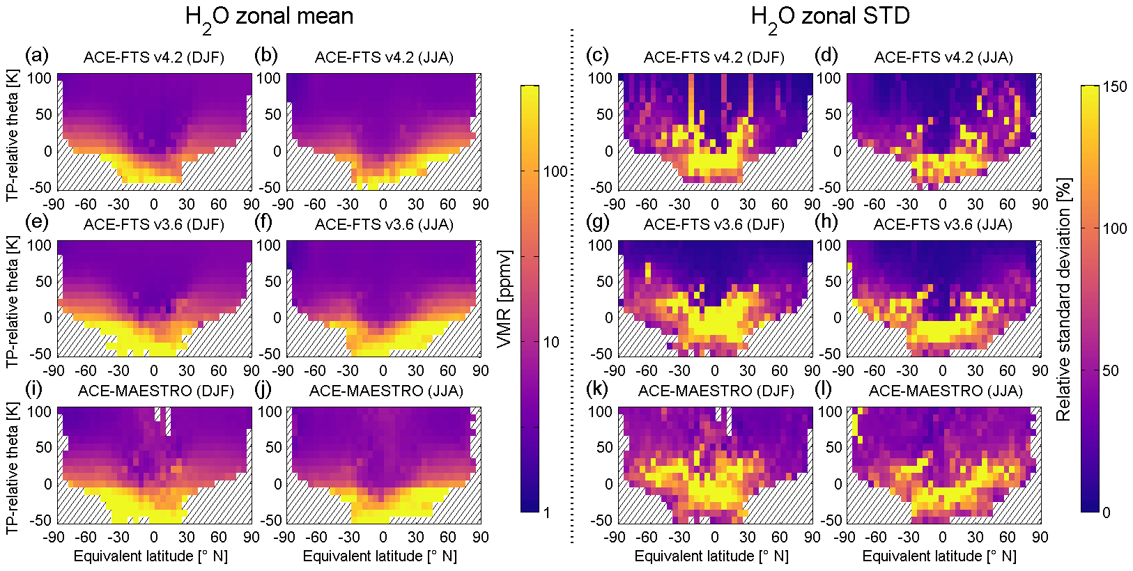
Figure 1 The 3-month zonal-mean multiyear-mean (June 2004 to May 2018) water vapour climatologies constructed from the ACE-FTS v4.2 (a–b), v3.6 (e–f), and MAESTRO (i–j) datasets for DJF (a, e, i) and JJA (b, f, j) in tropopause-relative potential temperature and equivalent-latitude coordinates. Also shown is the relative standard deviation for DJF (c, g, k) and JJA (d, h, l). Gaps in the data occur when there are either no observations made or fewer than five observations available for a given bin. Note the addition of hatching to the plots where there are no data available.

The meridional discontinuities in the vertical water vapour gradient, confined primarily to 10 K below to 50 K above the tropical tropopause, arise from a combination of transport effects. The regions of elevated water vapour in the midlatitudes and polar regions result from transport of water by the Brewer–Dobson circulation, while the comparatively reduced concentrations centered around the equatorial tropopause result from dehydration of air through the cold-point tropopause and subsequent transport of constituents away from the tropical UTLS region. The branches of the Brewer–Dobson circulation involved here are the lowermost branches, the transition and shallow branches, which propagate up to 70 and 30 hPa, respectively (Holton et al., 1995; Randel et al., 2006; Lin and Fu, 2013). Because tropopause-relative coordinates are used, the result of this dehydration and transport appears as a discontinuity in the VMR gradient in both sets of seasonal climatologies for all satellite datasets. Seasonal enhancement of water vapour, predominately in the troposphere but also over the lowermost 20–30 K of the stratosphere, is evident between the two sets of seasonal climatologies, with the summer hemisphere showing elevated water vapour concentrations compared to the winter hemisphere. This is influenced by the seasonal cycle in tropical cold-point temperatures and the decrease in saturation vapour pressure associated with lower temperatures in the winter that result in a reduced carrying capacity for water vapour in the winter hemisphere.

Some differences in variability are seen between the datasets (third and fourth columns in Fig. 1). The MAESTRO datasets show a larger relative standard deviation over much of the stratosphere than those from the two versions of ACE-FTS data, by over 50 % in the 50–100 K region in the summer hemisphere. ACE-FTS v3.6 has the largest region of high variability around the tropical tropopause, with a similar meridional extent to the high-variability region in the other datasets but a greater vertical extent in these features. It also displays the greatest variability in the approximately 30 K span directly above the tropopause in the winter hemisphere in the JJA climatologies. ACE-FTS v4.2 climatologies show some prominent features that are absent in the other datasets, namely the vertical lines near 30^∘ N/S in the DJF climatology and near 70^∘ N in JJA. This dataset also has the most tightly confined region of elevated variability near the tropical tropopause in both seasons. Despite these differences, broad consistency is seen in the distributions of relative standard deviation. In the area of greatest variability, centered around the tropical tropopause where there is vertical transport into the stratosphere, the consistency between measurement sets indicates that the source of this observed variability is related to underlying variations in vertical transport. Some regions of high variability extend from this region to higher latitudes in the extratropics, which is a consequence of wave-driven mixing, with asymmetry potentially stemming from hemispheric differences in the strength of this mixing. The appearance of these protrusions varies between the three datasets, indicating the potential influence of sampling biases related to the differences in the number and location of successful retrievals from each dataset. This will be explored further in the following section. Finally, the DJF climatologies show overall larger variability than that in the JJA climatologies.

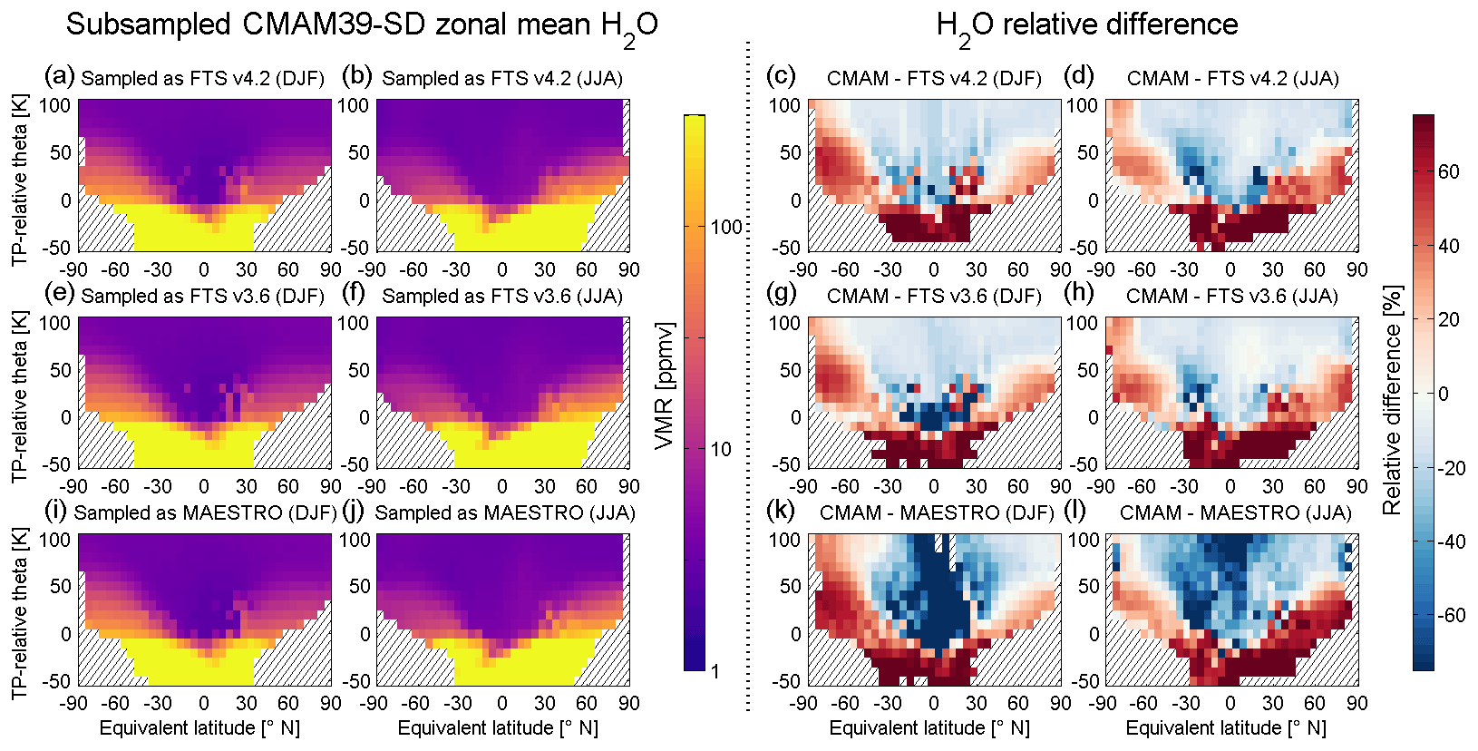
Figure 2 Comparisons between the CMAM39-SD model simulation, subsampled to the times and locations of the ACE-FTS v4.2 (a–d), ACE-FTS v3.6 (e–h), and MAESTRO (i–l) measurements and the satellite datasets. The zonal-mean multiyear-mean subsampled climatologies used for the comparisons are shown for DJF (a, e, i) and JJA (b, f, j), with the label in each plot giving the instrument measurement pattern the model is sampled with. Water vapour relative differences (%) between measurement climatologies and the CMAM39-SD reference climatologies calculated using Eq. (2), as outlined in Sect. 3.2, are shown in the third (DJF) and fourth (JJA) columns. The colour scale of the third and fourth columns is chosen to maximize visibility; however some extreme differences can be obscured by this choice. Note the addition of hatching to the plots where there are no data available.

4.2 Comparison

While many of the prominent features are present in the climatologies constructed from each dataset, they can vary, as shown in Fig. 2, which compares the climatologies constructed from CMAM39-SD, subsampled to the times and locations of the ACE-FTS v4.2, ACE-FTS v3.6, and MAESTRO measurements. The subsampled CMAM39-SD climatologies (Fig. 2, first and second columns) generally show patterns of water vapour that are consistent with the measurement climatologies, but there are large relative differences between the measurement and subsampled model climatologies (Fig. 2, third and fourth columns). Specifically, examining Figs. 1 and 2 shows significantly enhanced water vapour concentrations in CMAM39-SD over almost all of the troposphere and in the polar regions, as well as smaller water vapour concentrations near the tropical tropopause and over much of the stratosphere. The larger concentrations of CMAM39-SD water vapour in the polar regions are most prominent in the summer hemisphere and extend further into the stratosphere in the Southern Hemisphere during both seasons. These differences between the model and measurement climatologies ultimately play only a minor role in this study as the main use of CMAM39-SD is to compare the measurement datasets in a consistent fashion by accounting for sampling differences.

The CMAM39-SD subsampled model climatologies can be used to evaluate the influence of sampling on the measurement climatologies. To assess the portion of the differences between the measurement climatologies that arises from differences in sampling, whether from the measurement pattern or from the spatial and temporal distribution of successful retrievals, the sampling difference is evaluated by comparing the subsampled CMAM39-SD reference climatologies against each other, as shown in Fig. 3. Comparing these for water vapour shows that, over most of the UTLS, differences in the sampling pattern of ACE-FTS v3.6, ACE-FTS v4.2, and MAESTRO lead to only small differences in the climatologies for both periods, of approximately 4.2 % between the two ACE-FTS versions, 6.2 % between ACE-FTS v4.2 and MAESTRO, and 4.8 % between ACE-FTS v3.6 and MAESTRO, based on the average magnitude of the relative difference ($\left|\mathit{\delta }{r}_{i,j}\right|$, where the absolute value is taken to avoid oppositely signed differences cancelling each other out over the entire UTLS). These differences are heavily influenced by a few areas of poor agreement in the tropical upper troposphere and lower stratosphere, outside of which the agreement is typically found to be within 2 %. This is expected as the two instruments make simultaneous measurements, so their sampling patterns should only differ because of differences in their retrieval processes and success rate; however, the natural variability in water vapour can emphasize small differences in this, as seen around the tropics. DJF and JJA comparisons show similar results, with the JJA comparisons having slightly better agreement, by about 0.2 %–1.0 %. The upper troposphere shows larger absolute differences than those in the lower stratosphere, by about 3 %–5 % as averaged over the two regions. This comparison is influenced by the small differences previously noted near 50 K above the tropopause, which decreases the lower stratospheric average difference. Where large differences are observed, the greatest differences occur in the region spanning 0–20 K above the tropopause and approximately 15–30^∘ N. Over this small span, differences are mostly on the order of about 70 %, with one to two grid cells per comparison yielding differences in excess of 100 %, with these latter differences likely resulting from outlier measurements. Note that differences in excess of 40 % are not visible as the colour scale was chosen to emphasize differences over the entire UTLS at the cost of these large differences blending together. However, outside these few grid cells the subsampled model climatologies show overall excellent agreement, with differences of less than 5 %, indicating only a small sampling difference between the three water vapour datasets, as expected from their shared measurement pattern. Furthermore, the regions of greatest differences are coincident with the regions of highest variability, as shown in Fig. 1, a consequence of the range of VMR values observed in these regions and the impact of sampling on their averages.

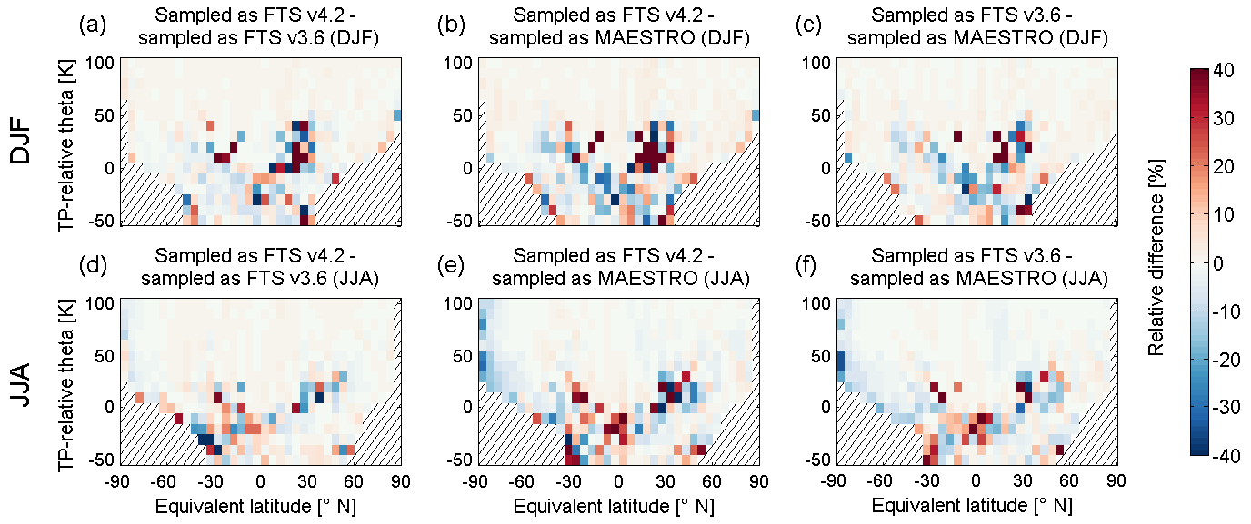
Figure 3 Intercomparisons of the CMAM39-SD model water vapour simulation, subsampled to the times and locations of the ACE-FTS v4.2, ACE-FTS v3.6, and MAESTRO measurements in order to assess the regions where the impact of the instruments' sampling pattern is largest. Panels (a–c) correspond to the comparisons for DJF, while panels (d–f) show comparisons for JJA. Each plot title gives the two subsampled climatologies compared, with differences given as a relative difference (%). These differences are calculated as the first subsampled model climatology minus the second and divided by the average of the two. Note the addition of hatching to the plots where there are no data available.

Table 1 Average magnitude of the relative differences ($\left|\mathit{\delta }{r}_{i,j}\right|$) in water vapour between the model and measurement climatologies over select regions of the UTLS. The approximate vertical region is denoted alongside the vertical range, with UT standing for upper troposphere and LS for lower stratosphere. The regions reflect where the model displays consistently higher or lower water vapour than the instruments. Values are bold if the instrument climatology yields more water vapour than CMAM39-SD for that period. In addition, the last row shows the average magnitude of the relative difference averaged over the entire UTLS but is not presented in bold to reflect the differing behaviour over the entire region. Differences are provided for DJF and JJA.

Having quantified the influence of the instruments' sampling patterns, focus can turn to comparing the measurement climatologies using the subsampled CMAM39-SD climatologies, in Fig. 2, as a reference. The average differences between the measurement and model differences are summarized in Table 1, separated by instrument and the regions discussed below, with the regions corresponding to swaths of the UTLS where the measurement–model comparisons display generally consistent behaviour. Over most of the upper troposphere, the subsampled CMAM39-SD climatologies yield elevated levels of water vapour compared to the three instrument climatologies, with differences of 65 % or greater. The three measurement climatologies were found to agree to within 4 % in DJF and 7 % in JJA, with better agreement found between ACE-FTS v3.6 and both other datasets than between ACE-FTS v4.2 and MAESTRO. The other regions in which CMAM39-SD has higher water vapour than the measurement datasets are the ranges polewards of approximately 45^∘ in each hemisphere and from 0–70 K above the tropopause. Over these two regions and periods, the agreement is variable, with agreement ranging from within 5 % in DJF to as large as 17 % in JJA (e.g., in the northern lower stratosphere). Altogether, these findings indicate that the satellite datasets are in generally good agreement across these regions. Note that there is a seasonal influence on the differences, with the measurements showing better agreement with CMAM39-SD and each other during the winter season in each hemisphere.

In the tropical lower stratosphere, the model-derived climatologies display smaller water vapour concentrations than those derived from the measurement datasets; this region also corresponds to where the poorest agreement is found between the satellite datasets. While the model–measurement differences for the ACE-FTS comparisons are between 15 %–25 %, the comparison with MAESTRO yields differences 2–4 times greater. The cause of this difference in the MAESTRO dataset is tied to the upper altitude bound of the MAESTRO water vapour retrieval, which is lower when the lower stratosphere is drier and vice versa, leading to observations of wetter conditions primarily populating higher-altitude locations, such as the tropical lower stratosphere. For ACE-FTS, the model–measurement comparison differences in the stratosphere during JJA are greatest over a region approximately 25^∘ wide, spanning 40 K in the vertical centered near 30^∘ S and 40–50 K above the tropopause. In DJF, the greatest difference between ACE-FTS v3.6 and the model occurs over an approximately 45^∘ and 30 K region centered around the tropical tropopause, while for ACE-FTS v4.2 only a few grid cells in this region show large differences. Because of the greater consistency in JJA than in DJF, the two versions of ACE-FTS are in better agreement in the former period than in the latter, with the former agreeing to within 5 %, while the latter shows differences of 8 %. In contrast, the large model–measurement differences displayed in the MAESTRO comparisons are not nearly as spatially limited and align poorly with the two versions of ACE-FTS studied. This apparent overabundance of MAESTRO water vapour in the tropical lower stratosphere, as compared to both CMAM39-SD and ACE-FTS, varies between the two seasons shown, with more extreme differences observed over a larger portion of the lower stratosphere in DJF than in JJA. Thus poor agreement, with differences of 22 %–66 %, is found between the two versions of ACE-FTS and MAESTRO over this region, but within this large range of differences the agreement in the JJA climatologies is significantly better than that in the DJF climatologies by about 40 %.

In spite of the discrepancy between water vapour in the model and satellite datasets, the subsampled CMAM39-SD model climatologies are valuable for assessing the impact of sampling. In this assessment, the measurement datasets show mixed relative performance, with the two ACE-FTS versions showing very good agreement throughout most of the UTLS, with differences of less than 10 %, while the MAESTRO climatologies show varied agreement with the two ACE-FTS versions, with differences ranging from less than 5 % to over 80 %, varying based on location and season. Part of the large difference seen in the MAESTRO comparisons results from the upper bound of the MAESTRO water vapour measurements near 22 km, where measurements tend to possess a high degree of uncertainty due to the worsening quality of MAESTRO water vapour retrievals with altitude. The altitudes included in these tropopause-relative climatologies are higher in the tropics than at the poles because the tropical tropopause is at higher altitude, so the lower-quality MAESTRO measurements from near its upper bound would have a larger influence in the tropics than at the poles in the lower stratosphere. The wet bias in MAESTRO water vapour found here agrees with estimates by Lossow et al. (2019) and Hegglin et al. (2021). In considering the entire UTLS, from 50 K below to 100 K above the tropopause, there is overall poor agreement between MAESTRO and ACE-FTS climatologies in DJF, with differences of approximately 40 %, but in JJA the overall difference is about 16 %, which is in much better agreement. Some regions of the UTLS show even better agreement, namely the upper troposphere and extratropical lower stratosphere, where the influence of the upper limit on the MAESTRO water vapour product is less impactful. Thus the MAESTRO dataset still provides valuable insight into water vapour in the UTLS, a finding supported by prior validation efforts (e.g., Lossow et al., 2019).

5 Ozone

In this section, the UTLS ozone climatologies generated from the ACE-FTS, MAESTRO, OSIRIS, and CMAM39-SD datasets are examined. The results shown are based on seasonal (3-month) climatologies for DJF and JJA.

5.1 Climatologies

Many features of the ozone measurement climatologies (first and second columns in Fig. 4) are broadly consistent, most notably the large gradient in the ozone VMR from a relatively uniform 0.05–0.1 ppmv below the tropopause to values nearly an order of magnitude greater above 70 K. This gradient arises because the tropopause acts as a transport barrier, largely confining higher ozone values to the stratosphere, while the reactivity of ozone as an oxidizing agent prevents it from becoming well mixed over time (Lelieveld and Dentener, 2000; Brasseur and Solomon, 2005). The observed vertical gradient in UTLS ozone is steepest in the tropics and the winter polar region, the two regions where the concentration of UTLS ozone is largest at the upper limit of the climatologies. These two local maxima arise from different processes, discussed in further detail below, with the underlying difference leading to the seasonal dependence of the polar ozone maximum location, as compared to the fairly static tropical feature.

Figure 4 Same as Fig. 1 but for ozone and including an additional row (m–p) for climatologies constructed from the OSIRIS dataset. The MAESTRO relative standard deviation is shown on a logarithmic colour scale in Fig. 7 to better illustrate the large values observed.

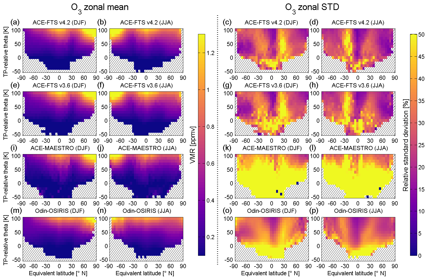
The tropical ozone peak is associated with the relative proximity of the tropical tropopause to the ozone concentration maximum in the tropical middle and upper stratosphere. Outside of the winter pole, the altitude of the ozone maximum in the mid-stratosphere somewhat mimics the shape of the tropopause, appearing lower in altitude near the poles as compared to the tropics; however this curvature is less pronounced than that of the tropopause. As such, outside of the winter pole, there is a greater difference in altitude between the ozone maximum and the tropopause at the poles than in the tropics. The result of this is the inclusion of air from nearer to the stratospheric ozone maximum within the upper bounds of the UTLS in the tropics but not to the same extent outside of this region. This directly leads to the larger concentration of ozone observed in Fig. 4 at higher altitudes in the tropics. The other key feature of these climatologies is the season-dependent stratospheric maximum over the winter pole, which extends further into the lower stratosphere than the tropical peak. Ozone is transported throughout the stratosphere via circulation processes, including those associated with the Brewer–Dobson circulation, with seasonal variations in these patterns leading to the observed enhanced ozone feature over the winter pole. Specifically, within the winter stratospheric polar vortex, the diabatic descent of cold air masses as part of the meridional overturning circulation carries ozone downwards from higher in the stratosphere, enhancing the ozone concentration in the lower stratosphere during the winter months.

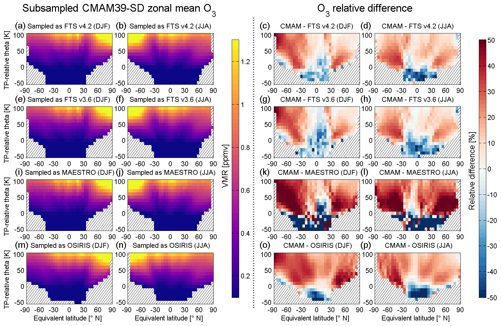
Figure 5 Same as Fig. 2 but for ozone and including an additional row (m–p) for climatologies constructed from the CMAM39-SD simulation subsampled to the location and time of the OSIRIS measurements and for the comparisons between these and the OSIRIS ozone climatologies.

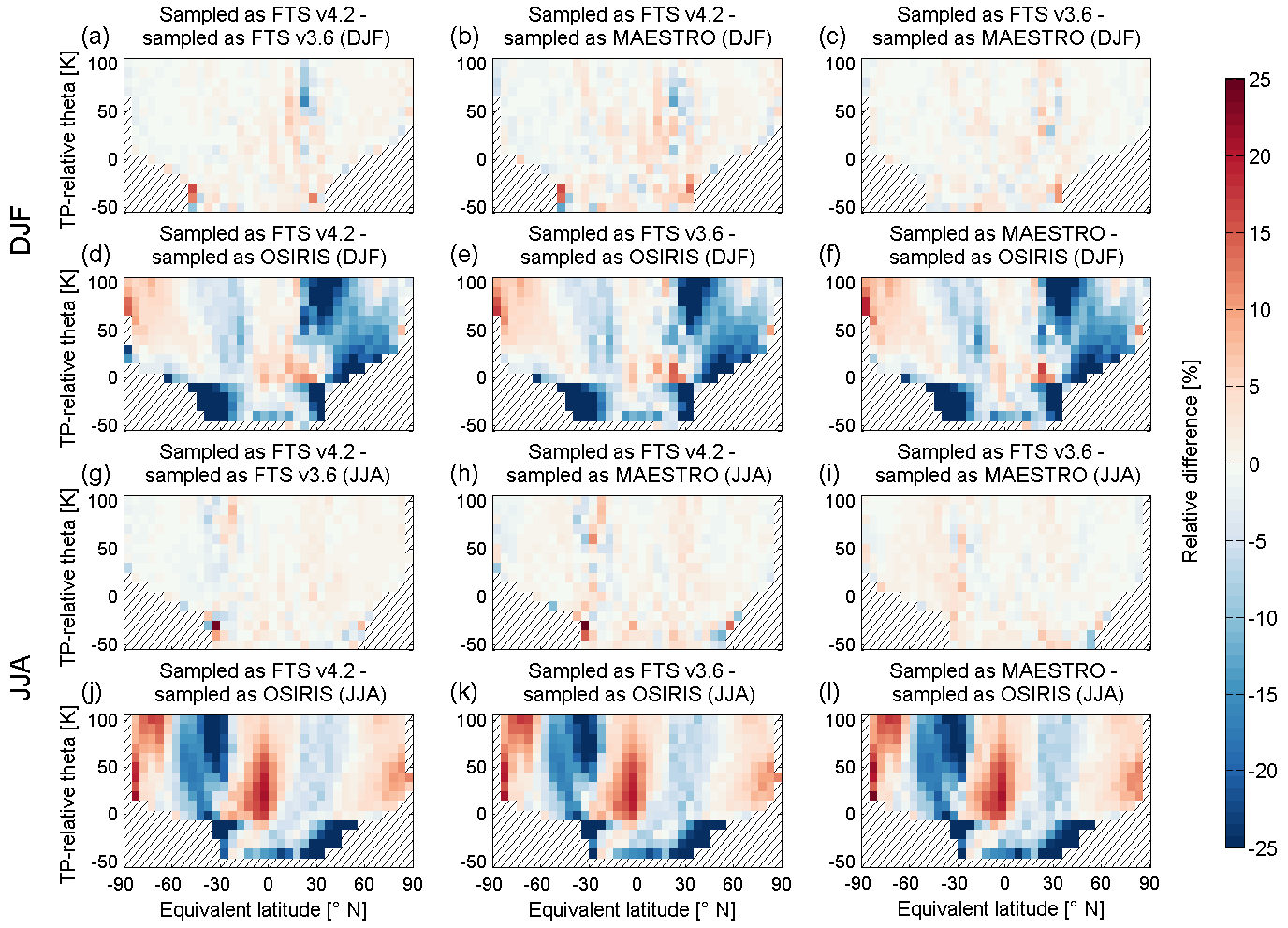
Figure 6 Same as Fig. 3 but for ozone and including an additional two rows for comparisons involving climatologies constructed from the OSIRIS measurement pattern. Note that the DJF and JJA comparisons are now spread over two rows each, with the top two rows corresponding to the former and the bottom two to the latter.

The aforementioned ozone features are present in all of the satellite climatology datasets, but there is variation between their appearance in each. Polar ozone is similarly distributed for the two ACE-FTS climatologies, but the MAESTRO distributions display a somewhat reduced feature and OSIRIS a still smaller feature. These features in the MAESTRO and OSIRIS climatologies are found to both cover a narrower meridional swath and extend less deeply into the UTLS. As shown in the subsampled CMAM39-SD climatologies in Fig. 5 (first and second columns) and the comparison of the subsampled CMAM39-SD climatologies in Fig. 6, there is little variation in ACE-FTS and MAESTRO sampling of this feature, indicating that this difference is most likely related to the ozone products themselves. Part of the product difference might be attributable to the higher vertical resolution of the MAESTRO instrument compared to that of ACE-FTS, but this cannot be disentangled from other potential sources for this discrepancy. The OSIRIS sampling pattern, in contrast, does lead to changes in the appearance of the polar ozone distribution, likely accounting for at least a portion of the reduced size observed for this feature. The tropical maximum also varies between the climatologies, appearing largest for ACE-FTS v3.6 and progressively smaller for ACE-FTS v4.2 and MAESTRO. The OSIRIS feature covers a smaller vertical range than that in the two ACE-FTS versions and a similar range to that from MAESTRO, but it extends further polewards than the other datasets and merges with the maximum over the polar region. While the depth of the tropical feature appears to be fairly consistent between the four sets of subsampled CMAM39-SD climatologies in Fig. 5, the extension of the high-ozone feature across the midlatitudes and into the polar region is seen only in the one set of subsampled CMAM39-SD climatologies, those subsampled to the OSIRIS measurement pattern, indicating that the feature is associated with sampling differences, which is supported by the comparisons shown in Fig. 6.

As with the distribution of mean ozone, the variability displayed by each set of climatologies (columns three and four in Fig. 4) is characterized by a series of broadly consistent features but with quantitative differences between the datasets. The general patterns of variability include two lower stratospheric regions of high variability, one in each hemisphere around 35^∘ N and 35^∘ S, that extend from the tropopause to the top of the UTLS climatologies and show more variability in the winter than in the summer hemisphere. These regions roughly border the edge between the upwelling and downwelling portions of the Brewer–Dobson circulation, so variable wave activity is a likely source of this variability as air parcels are sporadically mixed along isopleths (Plumb, 2002; Lin and Fu, 2013; Butchart, 2014). The appearance of the regions of highest variability is generally consistent between the two versions of ACE-FTS, but in the OSIRIS climatologies these regions are distributed over a larger meridional swath. In addition, the maximum values in these regions are smaller for the OSIRIS climatologies than for those derived from the two versions of ACE-FTS. Differences in the sampling patterns of each instrument are a likely cause of this difference between the datasets. High relative standard deviation values are also found in the troposphere for the ACE-FTS and OSIRIS climatologies, which may be influenced by there being fewer successful measurements by either instrument in this low-altitude region. This tropospheric variability extends to cover the entire troposphere in the OSIRIS climatologies while remaining concentrated near the tropics for ACE-FTS. The MAESTRO climatologies presented in Fig. 4 do not clearly display any of these relative standard deviation features; instead their variability distributions appear to be almost uniformly large throughout most of the UTLS when plotted using the same colour scale as for ACE-FTS and OSIRIS. Examining the distribution of MAESTRO variability in further detail on a logarithmic scale, as done in Fig. 7, reveals that it appears as a general gradient that decreases with altitude without much of the structure observed for other instruments, with the exception of the highest variability occurring near the tropical tropopause. As noted in Sect. 2.2, despite the filtering applied to the MAESTRO ozone dataset removing 8.9 % of the available profiles, the variability in the retrievals is too great to reliably identify all outliers. While this does not inhibit the use of MAESTRO in evaluating the consistency of these Canadian limb sounders, this does indicate that this v3.13 MAESTRO ozone product should be used with caution, in spite of the apparent agreement between most features of the ozone distributions derived from it and those from the other datasets employed in this study.

5.2 Comparison

The CMAM39-SD model dataset is used to evaluate the consistency between these measurement datasets as done for water vapour. Figure 5 shows DJF and JJA ozone climatologies generated from CMAM39-SD sampled to the times and locations of the ACE-FTS v4.2, ACE-FTS v3.6, MAESTRO, and OSIRIS measurements, as well as the comparison between these and the associated satellite climatologies. The subsampled model climatologies display very similar patterns in their ozone distributions to those in the measurement climatologies in Fig. 4, with the largest differences occurring in the summer hemisphere over the polar region where the model yields greater ozone VMRs above 60–70 K above the tropopause. The set of model–measurement comparisons (Fig. 5, third and fourth columns) further reveals that CMAM39-SD yields larger ozone concentrations than the measurement datasets outside the tropical lower stratosphere and smaller ozone concentrations than those datasets over the upper troposphere and in some instances in the tropical lower stratosphere. As with the water vapour comparisons, these differences between the model simulation and measurements do not limit the use of the model to evaluate the consistency of the measurement datasets.

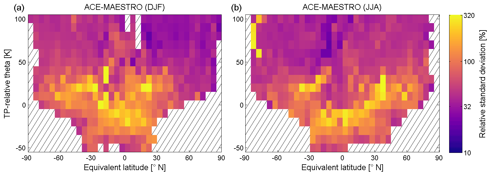
Figure 7 Alternative view of the MAESTRO ozone relative standard deviation, as first presented in Fig. 4k and l, with panel (a) here corresponding to Fig. 4k and likewise panel (b) corresponding to Fig. 4l. Note the shift to a logarithmic colour scale to better display the variability and the addition of hatching to the plots where there are no data available.

The subsampled CMAM39-SD climatologies in Fig. 6 aid in evaluating sampling effects. In evaluating the differences between the subsampled CMAM39-SD ozone climatologies, the average magnitude of the difference between the model climatologies generated using the times and locations of the ACE-FTS v4.2, ACE-FTS v3.6, and MAESTRO measurements is 1 %–2 %. The closest agreement for these three datasets, of 1.2 %, was found between the climatologies generated from the ACE-FTS v3.6 and MAESTRO measurement patterns, while the worst agreement, 1.7 %, was noted between the climatologies for ACE-FTS v4.2 and MAESTRO. Agreement is similar in the two seasons shown, with less than a 0.3 % change in the average comparisons between seasons. Thus their measurement patterns lead to negligible differences between the three datasets, with excellent agreement to better than 2 %, as expected for two instruments that share a line of sight for measurements of a gas that does not vary as extremely as water vapour. The subsampled model climatologies constructed using the OSIRIS sampling pattern were found to differ more greatly from those constructed using the sampling patterns of the other instruments, with differences on average of 9 % but as large as 76 % in the upper troposphere. The OSIRIS measurement pattern leads to alternating regions of larger and smaller concentrations, but the majority of these differences are constrained to the ±25 % range with better agreement found between the measurement patterns in the summer hemisphere. This generally fits with the finding of Sheese et al. (2021), where the 2σ geophysical variability in O₃ between coincident ACE-FTS and OSIRIS measurements was estimated to be on the order of about 5 %–50 % in the lower stratosphere, depending on latitude and coincidence criteria. Based on these comparisons, the OSIRIS measurement pattern leads to generally smaller concentrations of ozone in the upper troposphere. Overall, the OSIRIS measurement pattern leads to subsampled model climatologies that generally agree with the other three subsampled climatologies. In contrast to the results for water vapour, the ozone variability observed in Fig. 4 does not correspond to the regions of disagreement between the subsampled climatologies, indicating that the difference is mostly due to the sampling pattern rather than variability in ozone itself. Thus, this disagreement arises from differences between the two ACE instruments and OSIRIS in their latitudinal coverage and the timing of their observations throughout the two seasons analyzed.

Table 2 As in Table 1 but for ozone and with additional columns for the OSIRIS comparisons. Note that the regions marked with an asterisk (*) exclude the span from 5^∘ S–25^∘ N and 0–50 K.

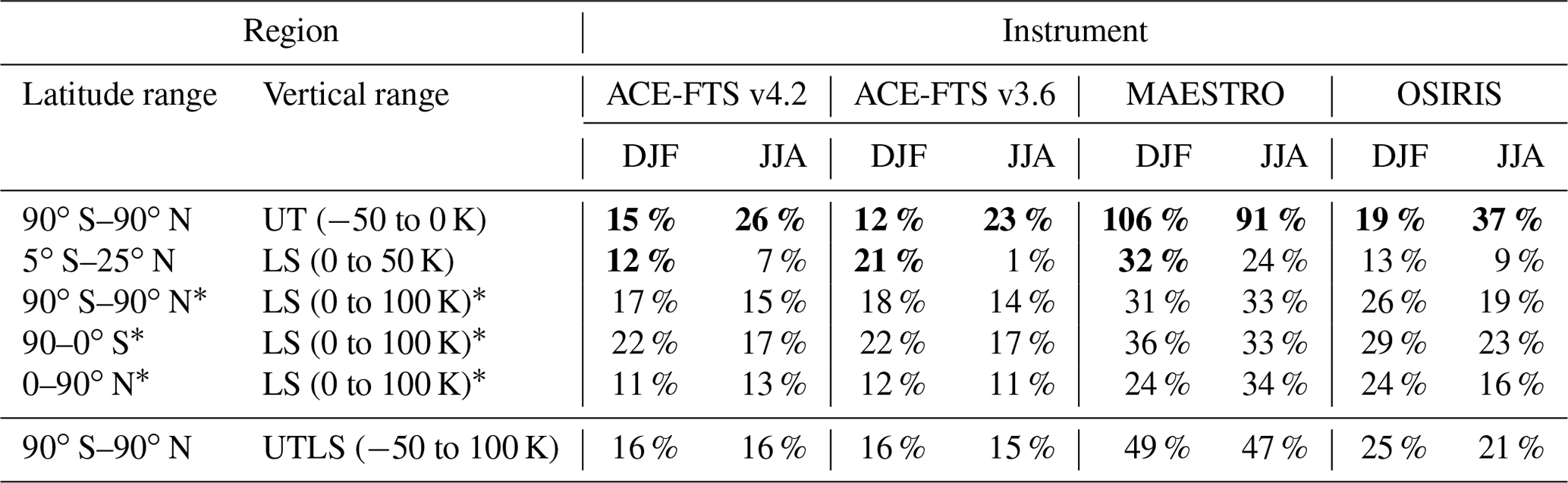
Focus can now turn to the comparisons between the instrument and the subsampled CMAM39-SD climatologies, shown in Fig. 5. The average differences between the measurement and model climatologies for regions of interest are presented in Table 2. It is immediately evident that the subsampled model yields smaller ozone concentrations than the measurements in the upper troposphere and larger concentrations in the lower stratosphere outside of the tropics. Below the tropopause, the model–measurement differences are largest for comparisons with MAESTRO and smallest for comparisons with the two sets of ACE-FTS climatologies, with the two versions of ACE-FTS agreeing to within 3 %, and OSIRIS agrees to within 11 % of ACE-FTS v4.2 and 14 % of ACE-FTS v3.6. In JJA the agreement between ACE-FTS and OSIRIS worsens, such that the differences are approximately twice as large as those in DJF. In contrast to this general agreement, MAESTRO ozone agrees poorly with the others below the tropopause, with the smallest difference being 54 %.

In the lower stratosphere, the subsampled model climatologies show generally larger ozone concentrations than the four measurement datasets, with exceptions within the tropics during DJF. Specifically, the subsampled model climatologies show smaller ozone VMRs than the ACE-FTS v4.2 and MAESTRO climatologies in DJF in the tropics between the tropopause and approximately 50 K above the tropopause, as well as with the ACE-FTS v3.6 DJF climatology up to about 100 K above the tropopause; however this difference is largest between the tropopause and about 50 K above the tropopause. For these three datasets, the differences occur primarily between about 5^∘ S and 25^∘ N, and successively greater ozone concentrations are seen in the ACE-FTS v4.2, ACE-FTS v3.6, and MAESTRO climatologies. The average model–measurement differences translate to ACE-FTS v3.6 agreeing with ACE-FTS v4.2 and MAESTRO to within 11 %, while the MAESTRO and ACE-FTS v4.2 climatologies show a 20 % general difference. The model comparison with the OSIRIS DJF climatology over this region leads to an oppositely signed difference, and thus the OSIRIS climatologies are in poor agreement with those from the other instruments, with the closest agreement, of 25 %, found between OSIRIS and ACE-FTS v4.2. In JJA the model yields generally greater ozone VMRs than the three ACE datasets, outside of a few grid cells, as it does in both seasons as compared to OSIRIS.

Outside the tropical lower stratosphere in DJF, the subsampled model climatologies generally display more ozone than the four measurement datasets in the lower stratosphere, with an exception for the region 0–20 K above the tropopause south of 60^∘ S, where the model exhibits less ozone than the measurements. For the regions where there is greater model ozone, model–measurement differences are larger in the Southern Hemisphere than in the Northern Hemisphere, with the MAESTRO comparisons showing the largest difference from the model while the two ACE-FTS versions show the smallest differences, in agreement with Hegglin et al. (2021). When averaged over the lower stratosphere, with the exception of the span between 5^∘ S and 25^∘ N noted above, the model–measurement comparisons imply agreement to within 2 % for the two ACE-FTS versions. The MAESTRO comparisons with the two versions of ACE-FTS yield differences of 13 %–23 %, with better agreement in DJF than in JJA by 2 %–10 %. OSIRIS typically agrees better with MAESTRO in DJF and with ACE-FTS in JJA; the DJF differences between MAESTRO and OSIRIS are less than 5 %, and those between OSIRIS and ACE-FTS are 8 %–13 %, while in JJA these differences are 10 %–18 % and 3 %–6 %, respectively.

In summary, the ozone climatologies from the satellite datasets show similar features, but there are moderate differences in their comparisons to CMAM39-SD and to each other. In the upper troposphere, the subsampled CMAM39-SD climatologies used for comparisons yield smaller ozone VMRs than those for the instrument climatologies, with the two versions of ACE-FTS displaying the least ozone, followed by the OSIRIS and then the MAESTRO climatologies, which yield the greatest VMRs. This is reversed over much of the stratosphere, except for a portion of the tropics where the model shows less ozone than three of the measurement datasets in DJF. Over the entire UTLS, from 50 K below to 100 K above the tropopause, with few exceptions, good agreement is found to within 10 % between the OSIRIS and ACE-FTS climatologies, while the MAESTRO ozone climatologies were found to agree fairly poorly with those from ACE-FTS and only somewhat better with those from OSIRIS, showing differences of between 31 %–33 % from ACE-FTS and of between 24 %–26 % from OSIRIS. While this disagreement is influenced by the large differences in the upper troposphere, MAESTRO is overall in the poorest agreement with the other datasets. This disagreement, coupled with the large variability observed for this product, supports the conclusion that the v3.13 MAESTRO dataset should be used with caution as it shows the least consistency with other instruments. In contrast, the results for the other three datasets demonstrate their value for UTLS ozone studies.

6 Summary

To meet the need for UTLS-focused climatologies, generated with the goal of minimizing the effects of geophysical variability and in support of the OCTAV-UTLS project, new climatologies have been constructed for water vapour and ozone from 14 years of data measured by three Canadian limb-sounding instruments: ACE-FTS (v3.6 and v4.2 water vapour and ozone), MAESTRO (v31 water vapour, v3.13 ozone), and OSIRIS (v5.10 ozone only). These climatologies use tropopause-relative potential temperature and equivalent-latitude coordinates in an effort to best represent the distribution of these two gases in the UTLS by accounting for some sources of variability (Pan et al., 2004; Hoor et al., 2004; Hegglin et al., 2008). The distributions of these two gases and their variability have been examined for two seasons, DJF and JJA. To evaluate their consistency in representing UTLS water vapour and ozone, these measurement climatologies have been compared to reference climatologies generated from the CMAM39-SD model, subsampled to the times and locations of the measurements made by each instrument. These subsampled model climatologies provide a consistent comparison reference to assess the agreement of the instrumental datasets, as well as to explore the influence of different measurement patterns on the datasets, but should not be considered to be a standard beyond this use.

In comparing the water vapour climatologies, overall differences of better than 8 % were found between the two versions of ACE-FTS. Agreement with MAESTRO was more varied, with comparisons against the two versions of ACE-FTS showing agreement ranging from less than 5 % to over 60 %, with the DJF climatologies showing typically poorer agreement than those for JJA. These comparisons are influenced by the upper bound of the MAESTRO water vapour product around 17–22 km and the large uncertainty associated with its measurements near this boundary. It should be noted that ACE-FTS v3.6 showed better agreement with MAESTRO than ACE-FTS v4.2 did; but this is influenced by the MAESTRO product using the v3.6 temperature and pressure information, which has been found to be the source of a drift in the ACE-FTS v3.6 data, thus leading to an expected drift in the MAESTRO data similarly to in the v3.6 data (Sheese et al., 2022).

Comparisons of the ozone climatologies yielded typically better agreement between the four measurement datasets than seen for water vapour. The two versions of ACE-FTS agree closely with differences of typically less than 2 %, and results for OSIRIS agreed with those from the two ACE-FTS climatologies with an overall difference of less than 10 %. As with water vapour, MAESTRO ozone was found to differ from the other datasets more significantly. MAESTRO showed the best agreement with OSIRIS, but overall differences were on the order of 25 %, and comparisons to ACE-FTS yielded agreement that was somewhat worse, by about 5 %–10 %, than with OSIRIS. Part of this disagreement stems from the MAESTRO ozone product displaying significantly higher variability than the other ozone datasets, preventing statistical filtering from reliably removing all outlier measurements using the method of Sheese et al. (2015), but overall the large disagreement suggests that the v3.13 MAESTRO ozone product should be used with caution.

In addition to assessing the agreement of the measurement climatologies, the subsampled model climatologies permit investigation into the influence of sampling patterns on the representation of water vapour and ozone in the UTLS. These subsampled model climatologies can be directly compared in order to determine where differences in sampling, whether from the measurement patterns or from the spatial and temporal distribution of successful retrievals, lead to differences in the climatologies. It was found that the high variability in upper tropospheric water vapour can lead to large differences even when comparing subsampled model climatologies generated from nearly identical sampling patterns, such as those for the two versions of ACE-FTS. Thus, even relatively small differences in sampling patterns can have a large effect on water vapour measurement climatologies in the UTLS. Contrasting this, the close agreement observed for the subsampled ozone model climatologies produced with similar sampling patterns indicates that mean ozone VMRs are less sensitive to underlying variability in ozone. However, differences in sampling patterns can still have a noticeable effect, such as the difference observed between the subsampled OSIRIS climatologies and those from ACE-FTS and MAESTRO. Overall, the choice of instruments employed in this study allows for the evaluation of key factors, namely atmospheric variability and sampling differences, that can influence differences in UTLS-focused climatologies of these species.