the Creative Commons Attribution 4.0 License.
the Creative Commons Attribution 4.0 License.
 | 01 Nov 2022
Exploring the link between austral stratospheric polar vortex anomalies and surface climate in chemistry-climate models
Nora Bergner
Marina Friedel
Daniela I. V. Domeisen
Darryn Waugh
Gabriel Chiodo
Extreme events in the stratospheric polar vortex can lead to changes in the tropospheric circulation and impact the surface climate on a wide range of timescales. The austral stratospheric vortex shows its largest variability in spring, and a weakened polar vortex is associated with changes in the spring to summer surface climate, including hot and dry extremes in Australia. However, the robustness and extent of the connection between polar vortex strength and surface climate on interannual timescales remain unclear. We assess this relationship by using reanalysis data and time-slice simulations from two chemistry-climate models (CCMs), building on previous work that is mainly based on observations. The CCMs show a similar downward propagation of anomalies in the polar vortex strength to the reanalysis data: a weak polar vortex is on average followed by a negative tropospheric Southern Annular Mode (SAM) in spring to summer, while a strong polar vortex is on average followed by a positive SAM. The signature in the surface climate following polar vortex weakenings is characterized by high surface pressure and warm temperature anomalies over Antarctica, the region where surface signals are most robust across all model and observational datasets. However, the tropospheric SAM response in the two CCMs considered is inconsistent with observations. In one CCM, the SAM is more negative compared to the reanalysis after weak polar vortex events, whereas in the other CCM, it is less negative. In addition, neither model reproduces all the regional changes in midlatitudes, such as the warm and dry anomalies over Australia. We find that these inconsistencies are linked to model biases in the basic state, such as the latitude of the eddy-driven jet and the persistence of the SAM. These results are largely corroborated by models that participated in the Chemistry-Climate Model Initiative (CCMI). Furthermore, bootstrapping of the data reveals sizable uncertainty in the magnitude of the surface signals in both models and observations due to internal variability. Our results demonstrate that anomalies of the austral stratospheric vortex have significant impacts on surface climate, although the ability of models to capture regional effects across the Southern Hemisphere is limited by biases in their representation of the stratospheric and tropospheric circulation.
- Article
(9051 KB) - Full-text XML
- BibTeX
- EndNote


Variability in the stratospheric polar vortex can influence surface climate on timescales of weeks to months (Baldwin and Dunkerton, 1999, 2001). For example, circulation anomalies during sudden stratospheric warmings (SSWs), events where upwardly propagating and dissipating waves rapidly decelerate the stratospheric zonal flow, can descend to the lower stratosphere and impact the tropospheric circulation. In the Northern Hemisphere (NH), where SSWs occur approximately every other year, these events are linked to surface extremes in midlatitude regions, for example cold-air outbreaks in North America and Eurasia (Scaife et al., 2008; Kolstad et al., 2010; Domeisen and Butler, 2020). In the Southern Hemisphere (SH), the polar vortex is stronger, less variable, and persists further into spring than its NH counterpart, and SSWs are very rare (2002 was the only recorded major SSW). These hemispheric differences are due to differing distributions of land surface and topography, resulting in weaker tropospheric wave disturbances in the SH (Plumb, 1989).
Despite major SSWs being extremely rare, the austral polar vortex shows some interannual variability, especially in late winter and spring, when increased insolation paired with stronger wave forcing lead to a more disturbed vortex. These polar vortex weakenings are similar to minor SSWs that also occur regularly in the Northern Hemisphere, where the zonal flow is weakened but complete wind reversal does not take place. Stratospheric polar vortex anomalies can influence the polarity of the Southern Annular Mode (SAM) in the troposphere (Thompson et al., 2005) and, as a result, can also affect SH surface climate. This influence is long lasting and extends to the entire late spring to summer season between October and January (Lim et al., 2018). For example, austral polar vortex weakenings have been suggested as drivers of surface extremes in southern and eastern Australia, enhancing the probability of hot and dry extremes and fire risk, with severe impacts for humans and ecosystems (Lim et al., 2019). This connection between perturbations in the wintertime to springtime polar vortex and subsequent surface climate shows the potential for the skillful seasonal prediction of both stratospheric and tropospheric conditions between August and February (Byrne and Shepherd, 2018; Lim et al., 2018; Domeisen et al., 2020). Enhanced predictability could improve early adaptation to reduce the negative impacts of extreme heat and drought on people and ecosystems. These vortex weakenings have also been linked to surface climate in Antarctica, with cooling over the Antarctic peninsula and warming over the rest of Antarctica (Kwon et al., 2020) that have potential knock-on effects on the ice sheet mass balance.
The vast majority of previous studies on SH stratosphere–troposphere coupling on interannual timescales have been based on station and reanalysis data. Even though some of the regional signals, such as the hot and dry extremes over Australia, have been extensively studied, the statistical uncertainty is large given the relatively short observational record in the SH and the small sample size of anomalous polar vortex events (depending on the definition, between 10–15 events; Lim et al., 2018, 2019; Byrne and Shepherd, 2018; Kwon et al., 2020). The robustness and spatial extent of the downward impact of the stratosphere in the SH thus remains unclear. Another observation-based method to investigate the robustness of a surface composite to sampling variability was applied by Oehrlein et al. (2021) for the NH SSW surface impacts. This method, based on bootstrapping, has been previously used to examine the extratropical response to the El Nino Southern Oscillation (ENSO) in the NH (Deser et al., 2017). Oehrlein et al. (2021) randomly resample observed SSW events to create synthetic bootstrapped surface composites that could have plausibly occurred with a different sequence of atmospheric variability unrelated to the polar vortex. They find that the pattern of synthetic composites is consistent with the known surface response to SSW's, but that the magnitude and spatial pattern is highly variable. They further find that the uncertainty in the SSW surface composite is largely independent from the strength of the stratospheric perturbation and results instead from internal tropospheric variability. Similarly, tropospheric variability may also play a role in regional signals observed after weak vortex events in the SH, but this is still unclear.
In contrast to observational data, climate model simulations offer the possibility to minimize the influence of internal tropospheric variability by using long ensemble simulations. Yet, models need to be able to simulate both a realistic mean state and variability to be valid tools. However, typical biases in climate models are a stratospheric “cold bias” in the SH and the resulting excessively strong and persistent stratospheric polar vortex (e.g., Butchart et al., 2011; Charlton-Perez et al., 2013; Lawrence et al., 2022). Models also have biases in the representation of the tropospheric circulation, such as in the position of the midlatitude jet; this may have consequences for the simulated tropospheric response to stratospheric perturbations, including those induced by ozone depletion and/or climate change (Gerber et al., 2008a; Wilcox et al., 2012; Simpson and Polvani, 2016). However, the implications of these biases for the downward impacts of stratospheric polar vortex anomalies in models are not yet fully understood.
In this study, we aim to explore the connection between polar vortex anomalies and the surface response to them in the SH in reanalysis data and chemistry-climate models (CCMs). In particular, we investigate the sensitivity of stratosphere–troposphere coupling and linkages to surface climate to internal variability and model biases. More specifically, we address the following questions. Can CCMs reproduce the surface climate response to polar vortex anomalies in the SH? Can CCMs help us to assess the robustness of the downward impacts of polar vortex anomalies, given the limited observational record? Which model biases can affect the representation of the tropospheric response?
We structure the analysis as follows: after presenting our data and methods in Sect. 2, we show and discuss the results of the stratospheric and surface signals of polar vortex anomalies in Sect. 3.1 and 3.2. We address the variability of the surface signal using bootstrapped surface composites in Sect. 3.3. Given the differences in surface signals across the midlatitudes between reanalysis data and our two CCMs, we address model biases in Sect. 3.4, revealing opposite biases in terms of the eddy-driven jet latitude and SAM timescales between the two models employed in this study. In Sect. 3.5, we compare our two CCMs with other simulations from the Chemistry-Climate Model Initiative (CCMI). Finally, we draw conclusions about our results in Sect. 4.
2.1 Data
For our analysis, we use the reanalysis Modern-Era Retrospective Analysis for Research and Applications version 2 (MERRA-2; Gelaro et al., 2017) for the time period 1980–2020, and time-slice simulations with two CCMs: the Whole Atmosphere Community Climate Model (WACCM) and the SOlar Climate Ozone Links model (SOCOL).
The variables of interest are the zonal mean geopotential height and zonal mean zonal wind, as well as surface variables: the sea-level pressure, 2 m temperature, and total precipitation. All data have been linearly detrended. When averaging over several latitudes, the data are weighted with the cosine of the latitude.
MERRA-2 is a global reanalysis dataset produced with the GEOS (Goddard Earth Observing System) atmospheric data analysis system using a three-dimensional variational algorithm with a 6 h update cycle. It spans the time frame from 1980 to the present and uses a finite-volume dynamical core at a resolution of 0.5∘ × 0.625∘ and 72 hybrid-eta levels from the surface to 0.01 hPa (Gelaro et al., 2017).
SOCOL is a coupled CCM that consists of the middle-atmosphere general circulation model MA-ECHAM (Middle Atmosphere European Centre/Hamburg Model) and the chemistry-transport model MEZON (Model for Evaluation of oZONe trends) (Stenke et al., 2013) and is coupled to the ocean–sea-ice model MPIOM (Max Planck Institute Ocean Model) by the OASIS3 (Ocean Atmosphere Sea Ice Soil) coupler (Muthers et al., 2014). It extends from the earth's surface to 0.01 hPa (approximately 80 km, has 39 vertical levels, and has a horizontal resolution of spectral truncation T31 (3.75∘ × 3.75∘). The chemistry-transport model includes 41 chemical species, determined by 140 gas-phase reactions, 46 photolysis reactions, and 16 heterogeneous reactions. Chemistry–climate interactions can be disabled by deactivating the coupling between chemistry and dynamics (Muthers et al., 2014). The model captures stratospheric variability reasonably well but shows a cold temperature bias at the pole and overestimates Antarctic total ozone loss during springtime (Stenke et al., 2013).
WACCM version 4 is a version of the National Center of Atmospheric Research (NCAR) Community Earth System Model (CESM1) that resolves the stratosphere and includes interactive chemistry (Marsh et al., 2013). It has 66 vertical levels, a model top at hPa (approximately 140 km), and a horizontal resolution of 1.9∘ latitude × 2.5∘ longitude. The model includes an active ocean and sea ice component with a nominal latitude–longitude resolution of 1∘. The chemistry module is based on the Model for Ozone and Related Chemical Tracers version 3 (Kinnison et al., 2007), and includes a total of 59 chemical species, 217 gas-phase reactions, and 17 heterogeneous reactions on 3 aerosol types. Like SOCOL, it can be run in a specified chemistry mode with prescribed instead of interactive chemistry (Smith et al., 2014). Stratospheric variability and the development of the ozone hole agree reasonably well with observations, but the model shows a cold pole bias (Marsh et al., 2013). The model has been used in several studies analyzing stratospheric variability and trends (e.g., Gillett et al., 2019; Haase and Matthes, 2019; Rieder et al., 2019; Oehrlein et al., 2020).
We use 200-year time-slice simulations from each model that are forced with constant boundary conditions of the year 2000. Seasonally varying greenhouse gas concentrations and ozone-depleting substances are fixed to this year. The quasi-biennial oscillation is nudged according to Stenke et al. (2013) in SOCOL and following Brönnimann et al. (2007) in WACCM. Both models have fully coupled dynamics, radiation, and chemistry, include ozone-circulation feedbacks and an interactive ocean, and therefore include various ENSO states and their impacts on the SAM, as in the reanalysis data. As our time-slice simulations contain neither climate change nor ozone depletion trends, they are well suited to investigating interannual variability. Hence, our simulations offer an unprecedented opportunity to investigate stratosphere–troposphere coupling under near-present-day conditions with a larger sample size than in the observations.
Additionally, we analyze ref-C2 simulations of CCMI models (Morgenstern et al., 2017) to corroborate the results obtained from the time-slice simulations. From the CCMI ref-C2 simulations, we use the models Community Earth System Model version 1 – Whole Atmosphere Community Climate Model (CESM1-WACCM), the Canadian Middle Atmosphere Model (CMAM), the ECHAM/Modular Earth Submodel System with 47 vertical levels (EMAC-L47MA) and 90 vertical levels (EMAC-L90MA), the Hadley Centre Global Environment Model, version 3 – Earth System (HadGEM3-ES), the L'Institut Pierre-Simon Laplace Coupled Model (IPSL), the Centre for Climate System Research National Institute for Environmental Studies Model for Interdisciplinary Research on Climate version 3.2 (CCSRNIES-MIROC3.2, two-member ensemble), the Meteorological Research Institute Earth System Model version 1 (MRI-ESM 1r1), the New Zealand National Institute of Water and Atmospheric Research – United Kingdom Chemistry and Aerosol model (NIWA-UKCA, five-member ensemble), and SOCOL3. These simulations are seamless simulations from 1960–2100, with ozone-depleting substances following the World Meteorological Organization (2011) A1 scenario and greenhouse gases following RCP 6.0 (Meinshausen et al., 2011). We only use the time period from 1980–2020 to be consistent with the time period of the reanalysis data. The models CESM1-WACCM, HadGEM3-ES, MRI-ESM 1r1, and NIWA-UKCA are coupled interactively to an ocean module, whereas, for the rest of the models, sea surface temperatures (SSTs) are prescribed from separate climate model simulations. More detailed descriptions of the models and simulations can be found in Morgenstern et al. (2017). We note that the design of the CCMI experiments (different SSTs across models, limited ensemble size, transient forcings, etc.) makes them less suitable to use to achieve the aim of this paper. Thus, the primary focus of our analysis is our time-slice simulations.
2.2 Methods
In the Southern Hemisphere, different methods have been used to identify strong and weak polar vortex events in previous studies. We choose a similar detection method to that in Thompson et al. (2005), based on the 10 hPa SAM. The SAM index is defined according to method 3 in Baldwin and Thompson (2009) as the principal component time series normalized to unit variance from the first empirical orthogonal function of daily, zonal mean geopotential height anomalies south of 20∘ S. Latitudinal weighting is applied as the square root of the cosine of latitude. The SAM index is calculated separately for all pressure levels and, by convention, a negative SAM index corresponds to positive geopotential height anomalies over the polar cap and weaker westerly zonal flow, and vice versa for a positive SAM index.
As the SAM variance peaks in austral spring, we detect the largest and smallest daily 10 hPa SAM index values between August and November each year. This method only allows for one weak or strong vortex event per year, which is reasonable as the dynamical timescales in the SH are long enough that the westerly flow remains weak/strong after a perturbation (Gerber et al., 2010). From these values, we define the highest and lowest 25 % as the strong and weak polar vortex events, respectively. Therefore, we obtain 10 strong/weak polar vortex events in the reanalysis data and 50 strong/weak events in the CCMs. We do not define a minimum temporal distance to the final stratospheric warming. For strong and weak polar vortex composites, we define onset dates as the time when the SAM value crosses +2 and −2 standard deviations, respectively, prior to the peak magnitude of the event (Thompson et al., 2005). The onset, peak timing, and magnitudes of the SAM index are documented for MERRA-2 in Table A1 in the Appendix.
The annular mode timescale is an integrated measure of annular mode variability and serves as an estimate of the persistence of annular mode anomalies (Gerber et al., 2010). We compute the SAM timescale as a function of season and height to quantify the persistence of SAM anomalies in the stratosphere and troposphere. SAM timescales are measured by the lag time (in days) that the SAM autocorrelation function takes to drop to . For the calculation, we use the methods described in Gerber et al. (2008b) and Simpson et al. (2011) for the SAM index by performing the following steps at all pressure levels:
-
The autocorrelation function (ACF) of the SAM is calculated for every day of the year d and lag l using the function
where y is the year and Ny is the number of years.
-
The ACFs are then smoothed with a Gaussian filter with standard deviation σ=18.
-
The e-folding timescale τ is estimated by applying a least-squares fit of the exponential function to the ACF up to lag l=50 (Gerber et al., 2008a).
We define the daily jet latitude index of the tropospheric eddy-driven jet as the location of the maximum 850 hPa zonal mean zonal wind between 35 and 70∘ S (Byrne et al., 2019) interpolated to a latitudinal grid of 0.1∘. Note that we use the terms “midlatitude jet” and “eddy-driven jet” interchangeably.
Daily anomalies are calculated by subtracting the climatology of each day of the year, which is computed by averaging over all available years for each calendar day. The climatology is therefore calculated for the period 1980–2020 in the reanalysis data and over the 200 model years in the CCM simulations.
We perform a one-sample bootstrapping test to estimate the significance of the time–height and surface composites. The composites based on the detected polar vortex events are compared to a distribution of 1000 random composites. These are created by sampling random years for the central dates in the time–height composites and random October-to-January periods for the surface composites, respectively. The actual composite is significantly different from 0 when it differs more than 2 standard deviations from the mean of the random distribution, which corresponds to a significance level of 95.5 %.
To estimate the uncertainty of the surface signal and to what extent it is affected by sampling variability, we use the bootstrapping method of Deser et al. (2017) and Oehrlein et al. (2021). The observed composite consists of 10 events with tropospheric states that are unrelated to the stratospheric signal. We randomly resample the 10 observed events with replacement to form 500 synthetic composites consisting of different combinations of the observed events, by necessity repeating some events and leaving other events out. In the synthetic composites, we allow an individual event to be repeated a maximum of three times. We thereby estimate how much the surface signal varies between the synthetic composites and how it relates to the strength of the polar vortex anomaly. Similarly, we generate 500 synthetic composites from the CCM data, randomly sampling 10 out of the 50 weak polar vortex years to obtain composites of the same size as in the observations, and also assess their relationship to the strength of the stratospheric anomalies.
We focus on the regional surface signals in Australia and Antarctica, as these are shown to be affected by polar vortex anomalies. We assess the variability across composites in these regions and calculate the area-weighted averages for:
-
The surface temperature in Antarctica: 65–90∘ S, excluding the Antarctic Peninsula region: 30–100∘ W
-
The surface temperature in Australia: 20–40∘ S, 113–154∘ E.
3.1 Stratospheric signal
To explore the range of the SH polar vortex variability in spring, we analyze the 10 hPa SAM. The SAM is directly related to zonal mean wind and is thus a valid metric of the polar vortex strength. The 10 hPa SAM distributions of the largest 25 % of the positive and negative daily polar vortex anomalies from August to November are shown in Fig. 1. The strongest polar vortex in the observations occurred in 2020, when the SAM index exceeded 4 standard deviations. The weakest polar vortex events in the observations occurred in 2002 and 2019, with SAM values below −9 standard deviations. Neither model reproduces the two most negative SAM events in the reanalysis, although the SAM anomalies in the models get reasonably close (−7 in WACCM and −8 in SOCOL). The inability of the models to capture extremes beyond 9 standard deviations may be due to the strong polar vortex bias in both CCMs. In WACCM, part of the reason may also be the weaker tropospheric wave forcing, as revealed by the smaller 100 hPa eddy heat flux anomalies near the onset date in this CCM (Fig. A3). An inability to reproduce the most extreme negative SAM events is a common feature of CCMI models (Fig. A6). However, the two models used in this study are among the CCMs that best capture extreme stratospheric SAM anomalies. Notably, both our CCMs reproduce the stratospheric SAM anomalies reasonably well, namely the asymmetry in SAM anomalies, with larger negative anomalies, and the bulk of the weak events overlap with the observations, similar to other CCMI models (Fig. A6).
We create composites of the SAM indices to compare the time and height evolutions of the weak and strong polar vortex events between the reanalysis and CCMs, as shown in Fig. 2. The anomalies peak in the mid- to upper stratosphere following the onset date (by construction) and persist in the lower stratosphere for up to 90 d (Fig. 2a, b), consistent with similar previous observational analyses (Thompson et al., 2005; Byrne and Shepherd, 2018). Stratosphere–troposphere coupling is apparent in all datasets, as the tropospheric signal after the onset of the peak stratospheric vortex anomaly tends to be of the same sign as the lower stratospheric anomaly. The time period of statistically significant downward impact is intermittent and does not exactly match between the datasets. While for weak vortex events, for example, the tropospheric signal peaks at days 30–60 in MERRA-2, the stratosphere–troposphere coupling is stronger and longer lived in SOCOL, resulting in a tropospheric signal that is more significant and persistent. Conversely, WACCM exhibits weaker and shorter-lived tropospheric anomalies.
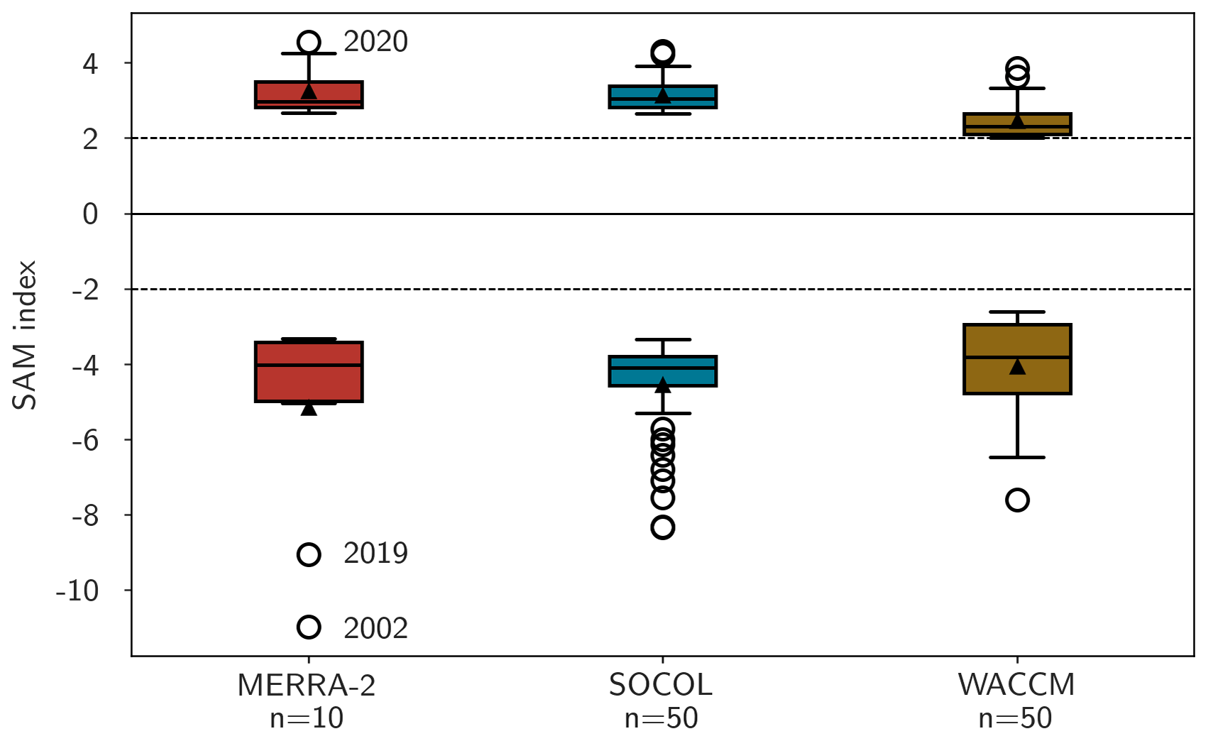
Figure 1The 10 hPa SAM index values of the lowest and highest 25 % of the springtime SAM indices in MERRA-2 (10 events per weak/strong category) and in the CCMs WACCM and SOCOL (50 events per weak/strong category). The most anomalous events in the observations are annotated with the year of occurrence.

Figure 2Time–height development of the SAM index following weak and strong polar vortex events for the reanalysis MERRA-2 (a, b), and the CCMs SOCOL (c, d) and WACCM (e, f). The central date (lag 0) refers to the first day when the 10 hPa SAM values have fallen below −2 and above +2, respectively. The indices are nondimensional and stippling refers to significance at the 4.5 % level assessed with a bootstrapping test.
3.2 Tropospheric SAM and surface climate
By exploring the time–height development of weak and strong polar vortex events, we have established that the persistent weak and strong anomalies in the lower stratosphere are associated with a tropospheric SAM of the same sign in the reanalysis and CCMs. We now further investigate the impact of the polar vortex anomalies on the troposphere and surface climate in the austral spring–summer season from October to January, as in Lim et al. (2018, 2019). We use the term “regime” to refer to the tropospheric pattern emerging after the weak and strong polar vortex events.
To examine how the tropospheric SAM differs between weak and strong polar vortex events, we compare the distribution of the average October to January SAM index at 500 hPa between models and the reanalysis (Fig. 3). The tropospheric SAM is on average negative following weak polar vortex events, in contrast to the positive SAM index that follows strong polar vortex events. In all datasets, the distributions of weak and strong polar vortex regimes are significantly different from each other based on a two-sided Student’s t-test at the 5 % level. However, the magnitude of the SAM response for both weak and strong polar vortex regimes differs among datasets. In the reanalysis, there is an asymmetry in the response, with a more strongly negative average SAM index during weak polar vortex regimes as compared to the magnitude of the SAM anomalies for strong polar vortex regimes, which is consistent with the asymmetry in stratospheric anomalies and therefore downward coupling (Fig. 1). In SOCOL, the average tropospheric SAM response for weak and strong regimes is more symmetric and of higher amplitude than in the reanalysis. The tropospheric SAM response in WACCM is much smaller for both weak and strong polar vortex years. The larger shift in the tropospheric SAM distributions in SOCOL compared to all other datasets is consistent with the stronger stratosphere–troposphere coupling in this model, as seen in the time–height development in Fig. 2. Conversely, the smaller shift in WACCM is consistent with the weaker stratosphere–troposphere coupling in this model.
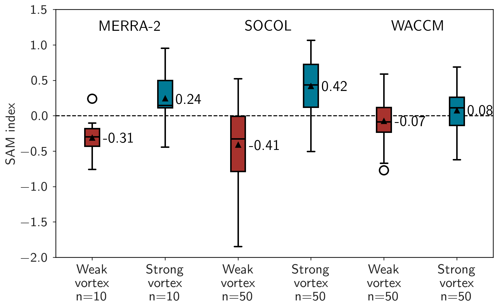
Figure 3Distribution of the mean 500 hPa SAM index averaged over the October–January period following weak and strong polar vortex anomalies for MERRA-2, SOCOL, and WACCM. Each box extends from the lower to the upper quartile of the data, and its whiskers extend from the lower quartile −1.5 IQR to the upper quartile +1.5 IQR. Data points outside of the whiskers are shown as circles. The horizontal line marks the median value and the triangle indicates the mean of the distribution, which is annotated next to the box.
Since the tropospheric SAM is known to modulate the surface climate in the SH midlatitude and polar regions (e.g., Hendon et al., 2007), we examine the surface patterns in October–January following stratospheric anomalies in the reanalysis and the CCMs. We primarily focus on weak polar vortex events, for which the observed tropospheric SAM response is larger than for strong polar vortex events, and which are associated with surface extremes in Australia in the following spring to summer (Lim et al., 2019). Anomalies associated with weak polar vortex regimes in sea level pressure (SLP), surface temperature, and precipitation are shown in Fig. 4 (strong polar vortex regimes are shown in Fig. A4 in the Appendix). The SLP composites show a large-scale pattern with positive pressure anomalies over Antarctica and negative pressure anomalies in midlatitude regions, consistent with the negative phase of the SAM displayed in Fig. 3. However, the magnitude and spatial extent of the SLP signal differ among the reanalysis data and model simulations, with WACCM showing a much weaker signal than SOCOL, consistent with the differences among these models in their tropospheric SAM responses (Fig. 3). Despite these differences, it is remarkable that both models and observations are consistent in exhibiting warm anomalies of up to 1 K over Antarctica.
In the midlatitudes, the surface signature of weak polar vortex events in temperature, SLP, and precipitation in MERRA-2 is remarkably similar to that seen in previous studies (Lim et al., 2018, 2019), despite the use of a simpler methodology in this paper (note that, in our study, we calculate the SAM index at every level independently and thus do not take the vertical covariance into account). However, MERRA-2 and the CCMs differ in both the magnitude and sign of the anomalies. For example, the CCMs do not show the warm and dry anomalies over southern and eastern Australia that are visible in MERRA-2. On the contrary, SOCOL shows cold temperature anomalies in southern Australia, while no significant signal is visible in WACCM over Australia and generally in the midlatitudes.
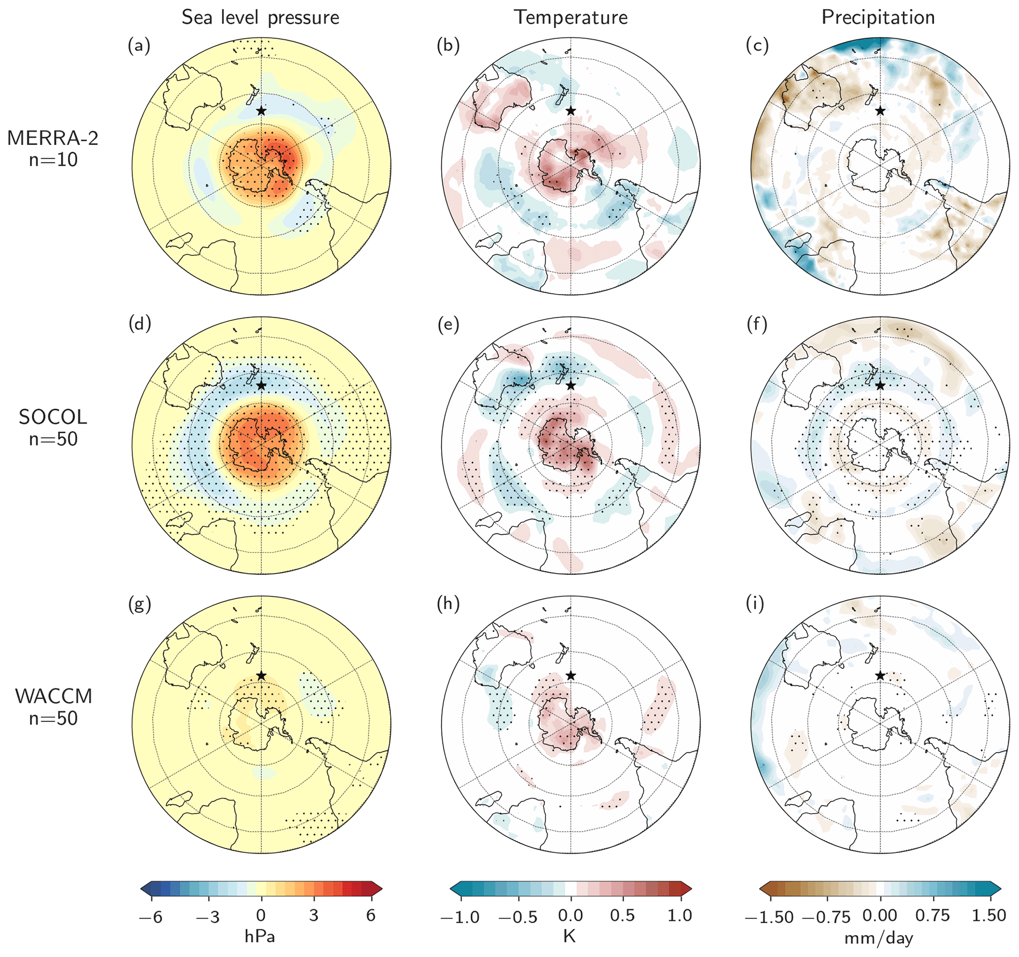
Figure 4Surface climate composites for weak polar vortex regimes of October–January SLP anomalies (a, d, g), 2 m temperature anomalies (b, e, h), and precipitation anomalies (c, f, i). The reanalysis data MERRA-2 (a–c) includes 10 weak vortex regimes, and the CCMs SOCOL (d–f) and WACCM (g–i) each include 50 weak vortex regimes. Stippling refers to significance at the 4.5 % level, assessed with a bootstrapping test.
3.3 Uncertainty in the surface climate response
In the previous sections, we have shown that some features of the modeled tropospheric and surface signals following weak polar vortex events do not resemble observations, especially in the midlatitudes. However, these signals may also be influenced by internal variability unrelated to the stratosphere. The question arises of how robust the observed tropospheric signal is, given the small number of observed events (n=10); hence, inconsistencies between reanalysis and CCMs could be due to a sampling issue. Figure 5 shows selected examples of surface temperature composites of random subsamples with 10 out of the 50 weak polar vortex regimes from the CCMs to be consistent with the sample size in reanalysis. In these subsamples, it becomes evident that the more zonally symmetric surface temperature anomalies in the CCM composites depicted in Fig. 4 arise from averaging over a larger sample size in the models. In the two examples shown in Fig. 5, the warming anomaly over Antarctica is robust across reanalysis and models. Conversely, the temperature anomaly over Australia varies among subsamples; in some of these subsamples, both models reproduce the observed warm anomaly (panels d, e), whereas in others, the models show cooling instead of warming (panels b, c).

Figure 5Examples of subsampled (n=10) temperature anomaly composites of weak polar vortex regimes for October to January for SOCOL (b, d) and WACCM (c, e), with the MERRA-2 (n=10) composite (a) shown for comparison.
We further examine the robustness of the observed and simulated surface responses to sampling variability in targeted regions (Australia and Antarctica, as marked in Fig. 5) and construct synthetic composites by randomly sampling 10 of the observed composites with replacement and by subsampling 10 of the 50 simulated weak polar vortex composites, following the same procedure as in Oehrlein et al. (2021). Figure 6 shows scatterplots of Australian and Antarctic temperatures and the stratospheric polar vortex strength (in terms of SAM anomalies at 10 hPa) in the 500 bootstrapped composites (n=10) in the reanalysis and CCMs. To the right of the scatterplot panels, the PDFs of the temperature distributions are shown for all 500 bootstrapped composites and all datasets.
We begin with the Antarctic temperature anomaly in Fig. 6a–d. In the reanalysis data, the sign of the Antarctic temperature anomaly in weak polar vortex regimes is robust, with 99 % of resampled composites showing warming, but there is a large spread in magnitude (Fig. 6b). The mean of the resampled composites is 0.3 K, with a standard deviation of 0.12 K. In the models, most subsampled composites also show Antarctic warming as a response to polar vortex weakening (95 % in SOCOL and 85 % in WACCM), highlighting the robustness of the warming signal over Antarctica after weak vortex events. Yet, the magnitude of this positive anomaly is subject to uncertainty, given the large spread in the magnitude of the subsamples in the reanalysis data as well as in the CCMs.
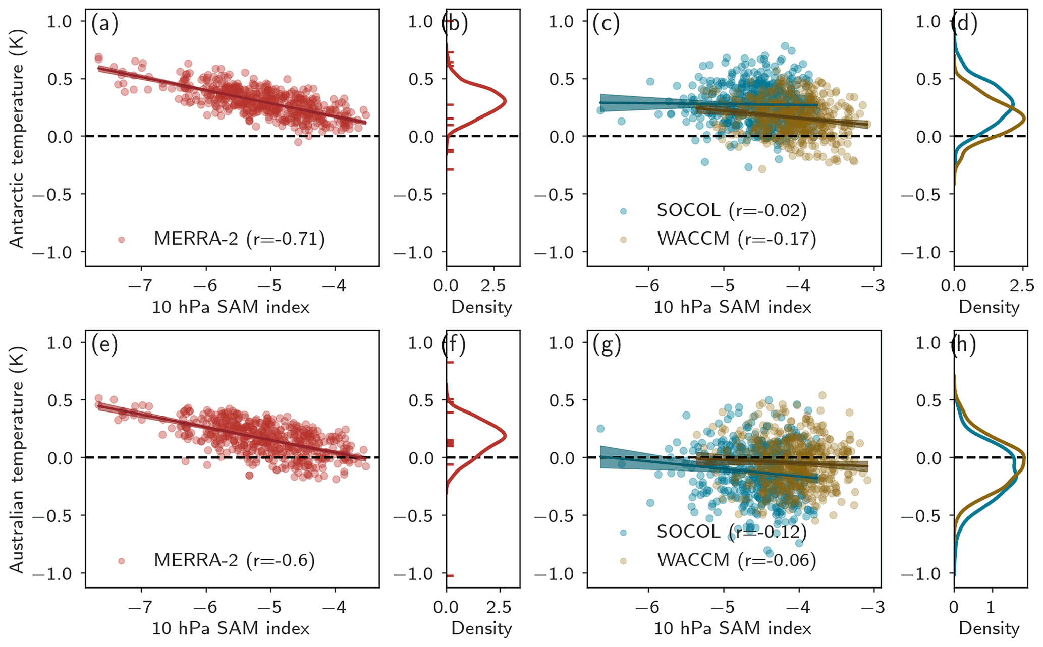
Figure 6Scatterplots of 500 synthetic bootstrapped composites (n=10) for Antarctic (a, c) and Australian (e, g) 2 m temperature anomalies in weak polar vortex regimes vs. the composite stratospheric 10 hPa SAM peak anomaly. The r value refers to the Pearson correlation coefficient between the two quantities. The line refers to the fitted linear regression and the 95 % confidence interval of the slope is shown as shading. The kernel density estimation (KDE) values of the temperature composites are shown on the right of the scatterplots (b, d, f, h), and the mean 2 m temperature values for the 10 weak polar vortex regimes are marked with red dashes for the reanalysis datasets.
In Australia, where 86 % of the bootstrapped composites in MERRA-2 show warming as a response to polar vortex weakenings, there are a wide variety of temperature responses in the CCMs. The average signal in WACCM is 0.05 K, with a standard deviation of 0.2 K. In SOCOL, the average of the synthetic composites is negative, with a mean of −0.13 K and a similar spread to that in WACCM with a standard deviation of 0.22 K. While the sign of the temperature response over Australia is largely robust in the reanalysis, the two models, on average, do not reproduce the observed warming following SH vortex weakenings.
The negative correlation between the Antarctic and Australian temperature anomalies and the stratospheric SAM in MERRA-2 shows that a good fraction of the variability in the surface temperature response is explained by the strength of the stratospheric perturbation. The correlation between surface signals and the magnitude of the stratospheric anomaly raises the question of how much the surface and bootstrapped composites are influenced by the two most extreme events, namely 2002 and 2019. When excluding these events, 95 % of the bootstrapped composites for the Antarctic surface signal still show a positive anomaly. This confirms the robustness of the sign of the Antarctic temperature response. Moreover, the uncertainty in the magnitude is related to the strength of the stratospheric anomalies, confirming a downward influence in the observations. Conversely, the magnitude of the stratospheric SAM anomalies is only very weakly correlated with the tropospheric signal in both CCMs, which suggests that internal (tropospheric) variability unrelated to polar vortex conditions accounts for most of the spread in the magnitude of the modeled signal.
In summary, the bootstrapped composites reveal a large uncertainty in the magnitude of the surface temperature response over Antarctica and Australia in both reanalysis and CCMs. However, while the Antarctic warming is evident in both observations and CCMs, the sign of the Australian temperature signal is only robust in the reanalysis, while there is no robust Australian temperature signal in the models. This suggests that the large differences in surface patterns between observations and models, as shown in Fig. 4, are unlikely to solely result from the short observational record and the limited number of observed SH vortex weakenings. Rather, differences between the PDFs of the bootstrapped temperature composites over Australia in Fig. 6 indicate systematic differences between the reanalysis data and the CCMs. One possible reason for these disagreements between models and observations is model biases, as assessed in the next sections.
3.4 Role of model biases in the simulated surface climate response
Given the differing surface impacts in both magnitude and regional extent between reanalysis data and CCMs, we first examine metrics characterizing the background state that are relevant for stratosphere–troposphere coupling.
We start with the climatology of the polar vortex and use 10 hPa zonal mean zonal wind at 60∘ S as a representation of the vortex strength. The mean annual cycle of the polar vortex is shown in Fig. 7a for MERRA-2 and the two CCMs. In both CCMs, the polar vortex shows a bias towards stronger zonal mean zonal winds and a later transition of westerly to easterly winds in spring. The strong polar vortex bias is particularly pronounced from June to January in WACCM. In this model, we even find years with year-round westerlies and no transition to easterly winds. The stronger westerly wind velocities in the models are likely one of the reasons for the inability of the models in capturing the most extreme weak vortex events (Fig. 1), as fewer planetary waves can propagate upward (Charney and Drazin, 1961).
Consistent with a strong vortex bias, the CCMs show very low stratospheric ozone variability (Fig. A2). Ozone feedbacks have also been suggested to be relevant for surface impacts (Hendon et al., 2020). In our models, the inclusion of interactive ozone has a significant impact on the evolution of the stratospheric SAM (not shown), but does not lead to significant differences in the troposphere (Fig. A1), suggesting that stratospheric ozone feedbacks are not critical for the representation of the surface response following stratospheric vortex anomalies in these two CCMs (see Sect. A1 in the Appendix). The smaller ozone variability in the models is thus unlikely to explain the inability of the models to reproduce some of the observed surface signals reported above.
The SAM in the troposphere is characterized by meridional vacillations of the midlatitude jet location (Thompson and Wallace, 2000), and is influenced by stratospheric variability (Fig. 2 and, e.g., Thompson et al., 2005). Moreover, the latitude of the tropospheric eddy-driven jet can also affect the strength of stratosphere–troposphere coupling, as shown in idealized model experiments (Garfinkel et al., 2013). By inspecting the climatological latitude of the eddy-driven jet in Fig. 7b, we seek to find reasons for the disagreement between modeled and observed surface patterns following weak polar vortex events (as seen in Fig. 4). It is readily apparent that there are opposite biases in the two models: in WACCM, the midlatitude jet is biased south, in contrast to a northward bias in SOCOL. While SOCOL deviates more from the reanalysis in the winter months than WACCM, it agrees better in the spring–summer season, which is the relevant time period for stratosphere–troposphere coupling in the SH. The jet in WACCM barely shows equatorward migration in the summer season, which is better represented in SOCOL.
Model biases in the jet position are consistent with the CCMs' tropospheric SAM surface patterns (Fig. A5). For example, as a northward shift of the eddy-driven jet implies a northward shift of the temperature patterns (and thus a northward shift of the warming signal over Australia, as in, e.g., SOCOL). Nevertheless, despite the CCMs' biases, the polar vortex perturbations project onto the tropospheric SAM, which is in line with the SAM response in very simple models (e.g., Domeisen et al., 2013).
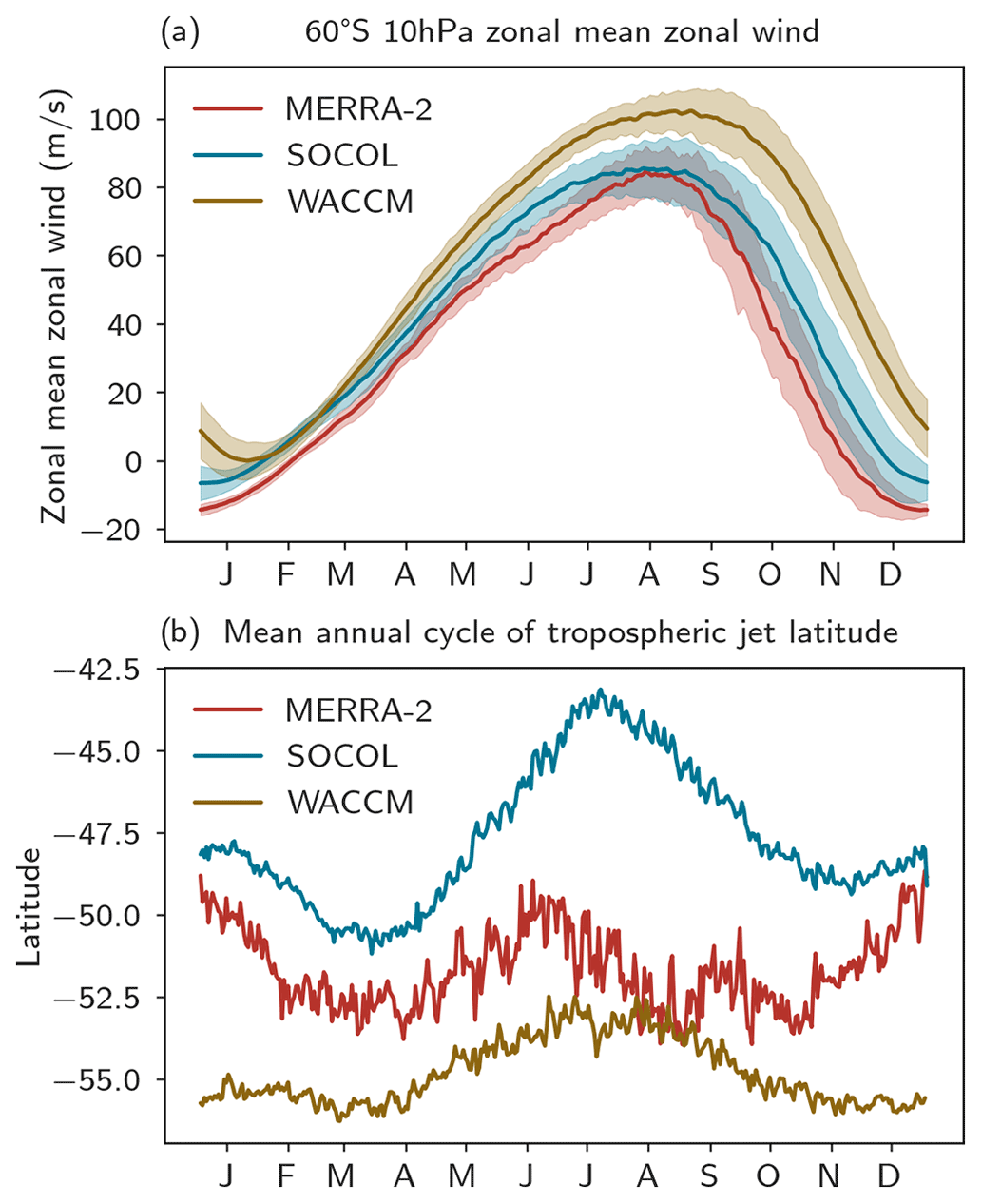
Figure 7Mean annual cycle of the 10 hPa zonal mean zonal wind at 60∘ S with the standard deviation (shading) (a), and the mean annual cycle of the daily jet latitude index, defined as the location of the maximum 850 hPa zonal mean zonal wind between 35 and 70∘ S for MERRA-2 and the CCMs WACCM and SOCOL (b).
Another indicator that tropospheric biases affect the downward response from the stratosphere is the persistence of the SAM, which is represented by the SAM timescales. This metric provides useful insights into the model's skill in representing low-frequency variability in the atmospheric circulation (Gerber et al., 2008b). An overestimated annular mode timescale implies that the modeled circulation may be overly sensitive to external forcings. Conversely, a short annular mode timescale in the troposphere is related to a small downward influence of the stratosphere (Gerber et al., 2008a; Chan and Plumb, 2009; Son et al., 2010). We show the SAM timescales as a function of season and pressure level in Fig. 8. Generally, anomalies in the SAM decay more slowly (and thus the timescale is longer) in the stratosphere than in the troposphere. While our two CCMs capture the general seasonal cycle of the SAM timescale, the stratospheric and tropospheric maxima are delayed compared to the reanalysis. The delayed seasonal cycle likely results from the strong vortex bias. Additionally, both models show a late spring polar vortex breakup compared to the observations, as seen in Fig. 7a, which might delay the seasonal cycle in the troposphere. Most remarkably, the SAM timescales in the CCMs differ in opposite ways with respect to the observations in the troposphere, with SAM timescales strongly overestimated in SOCOL – a typical bias of climate models in the SH (Gerber et al., 2010). In contrast, tropospheric SAM timescales in WACCM are shorter than in the reanalysis, particularly in spring to summer.
The opposite biases of tropospheric SAM timescales in the CCMs are consistent with their different eddy-driven jet locations (Fig. 7b). Climatological jet locations and SAM timescales are shown to be highly correlated, with lower SAM timescales for jet locations at higher latitudes (Son et al., 2010; Kidston and Gerber, 2010). The differing SAM timescales are related to eddy–mean flow feedbacks that are sensitive to the latitude of the eddy-driven jet (Son et al., 2007; Gerber and Vallis, 2007; Simpson et al., 2010). For example, eddy activity is confined to a relatively small latitudinal band of high baroclinicity at the edge of the Hadley cell for a more equatorward jet, which can make zonal mean flow anomalies more persistent.
Taken together, we have identified model biases in the tropospheric circulation, which are likely the reason for the disagreement between models and observations, namely the overestimation in the tropospheric response in SOCOL and the underestimation in WACCM in comparison with reanalysis data.
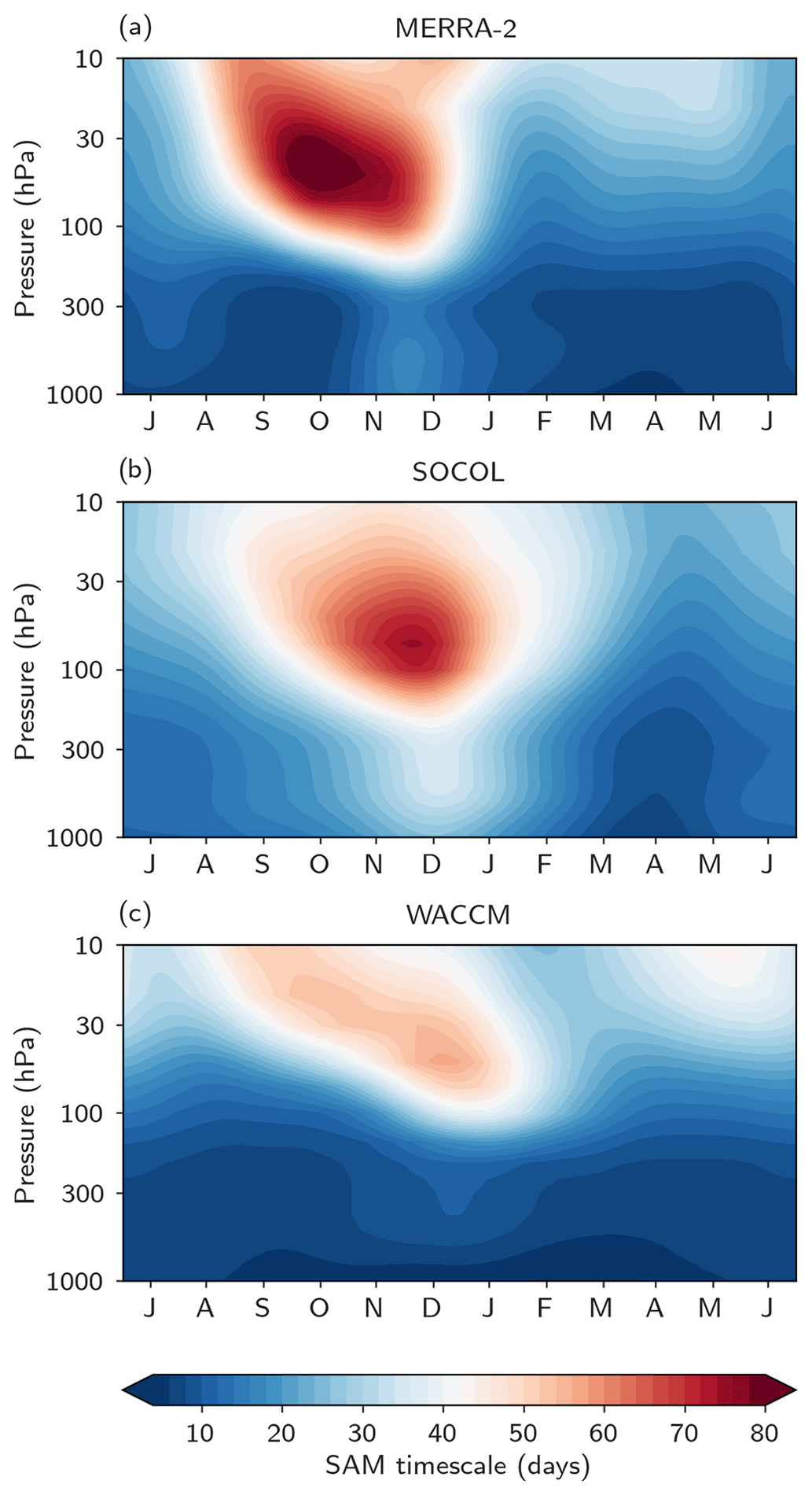
Figure 8The SAM timescale τ (in days) as a function of season and height in the reanalysis MERRA-2 (a) and the models SOCOL (b) and WACCM (c).
3.5 Comparison with CCMI simulations
To gain a better understanding of the relationship between model climatologies and stratosphere–troposphere coupling, we examine CCMI ref-C2 simulations over the historical period (1980–2020). The CCMI models show a similar spread of polar vortex events to the time-slice simulations from WACCM and SOCOL and reproduce the bulk of the observed composites, except for the two most extreme years (2002 and 2019) (Fig. A6). From Fig. A7, we can conclude that the CCMI models also show a clear tropospheric response in the October–January tropospheric SAM following weak polar vortex events (panel a), and most models show warm anomalies over Antarctica and Australia.
With the addition of the CCMI models, we confirm that the SAM timescale, particularly in the lower stratosphere, affects the magnitude of the tropospheric SAM following weak polar vortex events, as seen in the significant negative correlation between the mean October–January 50 hPa SAM timescale and the October–January 500 hPa SAM response (Fig. A7a). Also, the October–January surface temperature anomalies following weak polar vortex events in Australia and Antarctica are positively correlated with the lower stratospheric (50 hPa) SAM timescale (Fig. A7b and c), meaning that models with longer timescales tend to show a stronger warm anomaly in these regions. This is in line with previous findings in the Northern Hemisphere, showing that the persistence of circulation anomalies in the lower stratosphere is an important indicator of the magnitude of the surface response to SSW's (Runde et al., 2016; Karpechko et al., 2017).
On the other hand, the CCMI models do not clearly show any influence of the climatological jet latitude on the resulting surface temperature patterns (Fig. A7d). Some models show sizable warming over Australia (0.3–0.4 K) despite an even more biased midlatitude jet position than in our time-slice SOCOL experiments (e.g., CMAM, CCSRNIES-MIROC3.2). We note, however, that differences among CCMI models in their SSTs (some models used prescribed SSTs, while others used modeled SSTs) make direct comparisons difficult, as these likely influence the surface impacts as well. The model simulations that show reasonably similar surface responses compared to the reanalysis data are also closer to the reanalysis in terms of both jet latitude and SAM timescales (e.g., MRI-ESM1r1, NIWA-UKCA), even though there is substantial internal variability, as can be seen from the different NIWA-UKCA ensemble members. Overall, the CCMI models support our conclusion that a clear shift towards a negative surface SAM following weak polar vortex events can be seen, but that the magnitude of this signal is influenced by the model's representation of the SH stratospheric and tropospheric circulation.
In this study, we assess the role of interannual austral stratospheric vortex variability in forcing SH spring- and summertime surface climate. Based on the analysis of observational data and targeted CCM simulations, we have examined the downward impact of polar vortex anomalies on interannual timescales in the spring–summer season (October–January), confirming previous findings (e.g., Thompson et al., 2005; Lim et al., 2018, 2019; Kwon et al., 2020) and expanding on them as follows. The main results are:
-
The downward impact of the polar vortex can be seen in the subsequent shift of the tropospheric SAM to its negative/positive phase in weak/strong polar vortex regimes. Further, our observational analysis shows that the surface response to weak polar vortex events includes warming and dry conditions over Antarctica and Australia, confirming earlier studies. However, our results also show that while models robustly capture the warming signal over Antarctica, they struggle to reproduce the observed surface signal in the midlatitudes, especially over Australia.
-
An “observational large ensemble” analysis based on a bootstrapping method reveals that the observed warming signal over Antarctica and Australia is robust, although the magnitude of the signal is uncertain. In the model experiments, we find that the Australian temperature signal is very uncertain, with equal likelihoods of warming and cooling. Despite the short observational record and thus limited number of observed vortex weakenings in the SH, the reanalysis data reveal a surface signal that is more robust in its sign and more correlated to the stratospheric forcing than in the long-term modeling experiments. Thus, we exclude internal variability and any differences in the stratospheric variability as reasons for differences in surface signals between models and observations.
-
Biases in the polar vortex strength, eddy-driven jet location, and SAM timescales limit the models' ability to capture observed signals in midlatitudes. The bias in the surface impact of stratospheric circulation anomalies differs between models, with WACCM possibly underestimating and SOCOL overestimating the downward stratospheric impacts. We suggest that this is due to biases in the latitudinal location of the tropospheric jet and the SAM timescale, with WACCM having a poleward bias in the jet and a timescale that is too short, whereas the jet is biased equatorward and the SAM timescale is too long in SOCOL. The relationship between SAM timescale and surface signal is further confirmed by the CCMI models.
While the understanding of stratosphere–troposphere coupling and associated surface impacts has advanced in recent times, further research is necessary to gain a better understanding of the relevant processes and their representation in numerical models. Improving the representation of SH large-scale dynamics in the stratosphere and troposphere in models, as well as dynamical and ozone variability, is important for further investigating surface climate impacts associated with stratospheric forcings. Considering the ongoing changes in the stratosphere, with ozone recovery and increasing greenhouse gas concentrations, further work is necessary to better understand stratosphere–troposphere coupling and how it may change in the future on both long-term and interannual timescales.
A1 Ozone feedbacks
The SH tropospheric circulation is known to be sensitive to stratospheric ozone variations. Long-term ozone depletion has driven widespread surface climate changes (e.g., Thompson and Solomon, 2002; Thompson et al., 2011; Previdi and Polvani, 2014). Aside from long-term changes, a downward influence from the interannual variability of stratospheric ozone on spring to summertime surface climate has also been suggested (Son et al., 2013; Bandoro et al., 2014; Gillett et al., 2019; Damiani et al., 2020). However, dynamical and ozone variability are strongly linked and separating ozone feedbacks from dynamical variability is difficult. Including ozone feedbacks in weather and climate models may result in more accurate results, as has been shown for example for the 2002 SSW in the SH (Hendon et al., 2020). However, interactive ozone is also computationally expensive.

Figure A1Distribution of the mean 500 hPa SAM index averaged over the October–January time period following weak and strong polar vortex anomalies for MERRA-2 (a), SOCOL INT-O3 and CLIM-O3 (b), and WACCM INT-O3 and CLIM-O3 (c). Each box extends from the lower to the upper quartile values of the data, and its whiskers extend from the lower quartile −1.5 IQR to the upper quartile +1.5 IQR. Data points outside the whiskers are shown as circles. The horizontal line marks the median value and the triangle marks the mean of the distribution, which is annotated next to the box.
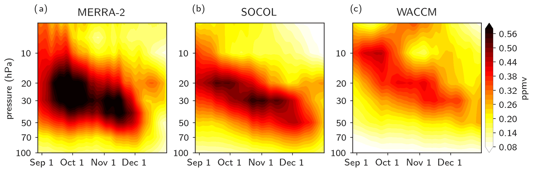
Figure A2Ozone standard deviation in austral spring in MERRA-2 (a), SOCOL (b), and WACCM (c).
To isolate the influence of ozone-circulation feedbacks, we compare simulations with fully interactive ozone to those with specified ozone chemistry. In the fully interactive ozone simulations (INT-O3), the free running models interactively calculate ozone concentrations, which allows direct feedbacks with radiation and dynamics. The runs with specified ozone chemistry (CLIM-O3) still interactively calculate ozone in the background, but ozone is decoupled from the radiation scheme and replaced with monthly mean zonal mean ozone climatologies derived from the 200-year long INT-O3 runs. For both models, the INT-O3 and CLIM-O3 simulations have 200 model years each.
In Fig. A1, we show the average tropospheric SAM in weak and strong polar vortex regimes from the simulations with interactive (as in Fig. 3) as well as climatological ozone. On average, model simulations with climatological ozone (which, by definition, do not include radiative/dynamical feedbacks from ozone) also show a negative tropospheric SAM during weak polar vortex regimes and a positive SAM during strong polar vortex regimes in October–January, similar to simulations including fully interactive ozone chemistry. We find small but significant differences in the magnitude and persistence of SAM anomalies between simulations including and excluding ozone feedbacks in the stratosphere (not shown). Conversely, ozone feedbacks have little effect on the tropospheric SAM signal and surface climate.
Taken together, these results suggest a dominant role of dynamical variability for stratospheric polar vortex extremes and their downward influence on tropospheric and surface climate, while ozone feedbacks only play a minor role in the downward coupling. However, the CCMs underestimate ozone variability, as shown in Fig. A2, possibly resulting in an underestimation of ozone feedbacks. Hendon et al. (2020) show the importance of stratospheric ozone for accurately simulating anomalies in the stratosphere and at the surface for the 2002 SSW. However, 2002 is the most extreme event in the observations and the absence of such high-amplitude perturbations in the CCMs may explain the missing contribution of ozone feedbacks to surface climate in the two CCMs considered.
A2 Additional information
Here we show the onset and peak dates as well as the peak amplitudes of polar vortex events in MERRA-2 (Table A1). Additional figures include the eddy heat flux composite for MERRA-2 and the two CCMs in Fig. A3, the surface climate composites of strong polar vortex regimes for surface pressure, temperature, and precipitation anomalies in Fig. A4, the regression of 2 m temperature on the 1000 hPa SAM in Fig. A5, the anomalous stratospheric SAM indices in the CCMI models in Fig. A6, and relationships between the SAM timescale, latitudinal jet locations of CCMI models, and surface climate following weak polar vortex events in Fig. A7.
Table A1Details on the timing and magnitudes of the detected weak and strong polar vortex events in MERRA-2 used in this study. Peak amplitudes are in standard deviations and refer to the SAM index at 10 hPa.
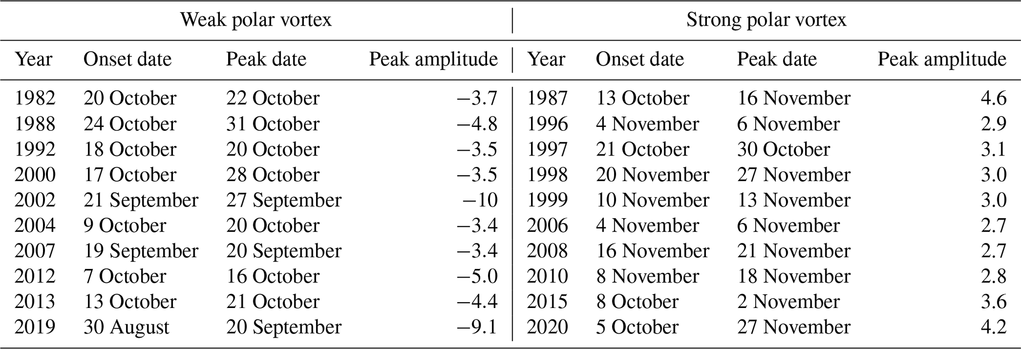

Figure A3Composites of eddy heat flux anomalies (K m s−1) averaged over 45–75∘ S at 100 hPa for strong and weak polar vortex events for MERRA-2 and the CCMs SOCOL and WACCM. The central date (lag 0) refers to the onset day of the polar vortex anomaly.

Figure A4Surface climate composites for strong polar vortex regimes for October–January SLP anomalies (a, d, g), 2 m temperature anomalies (b, e, h), and precipitation anomalies (c, f, i). The reanalysis data MERRA-2 (a–c) includes 10 weak vortex regimes, and the CCMs SOCOL (d–f) and WACCM (g–i) each include 50 weak vortex regimes. Stippling refers to significance at the 4.5 % level assessed with a bootstrapping test.

Figure A5Regression of daily 2 m temperature anomalies on the daily 1000 hPa SAM index for the October to January time period for the reanalysis data MERRA-2 (a) for the time period 1980–2020 and the CCMs SOCOL (b) and WACCM (c) for 200 model years each.
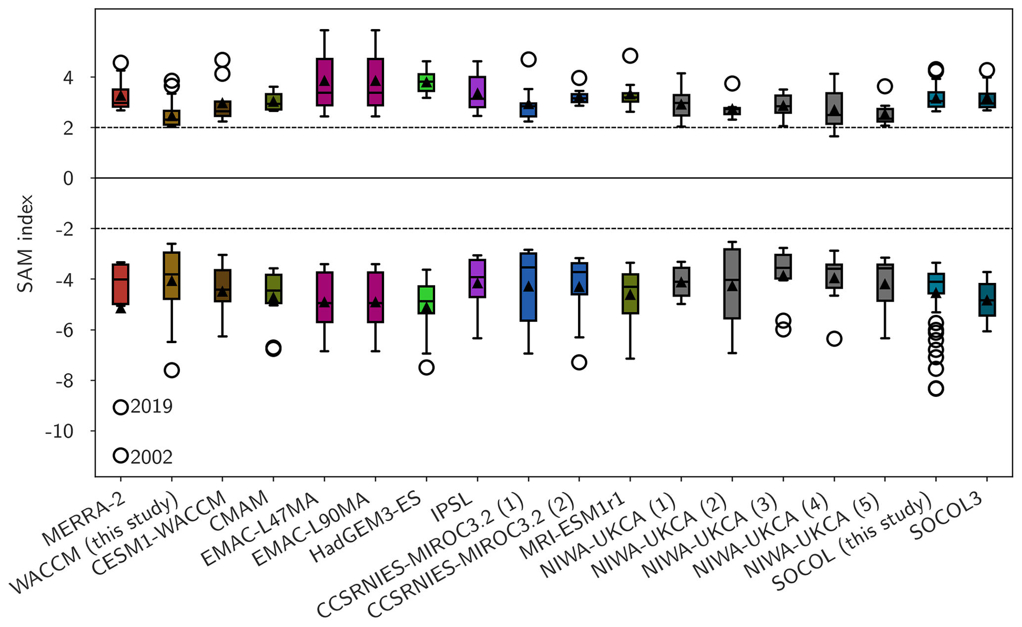
Figure A6The 10 hPa SAM index values of the lowest and highest 25 % of the springtime SAM indices in MERRA-2 and the CCMI models (10 events per weak/strong category) and in the time-slice simulations of WACCM and SOCOL (50 events per weak/strong category).

Figure A7The mean October–January 50 hPa SAM timescale in each model and the reanalysis data versus the mean October–January 500 hPa SAM response (a), Antarctic temperature anomalies (b), Australian temperature anomalies (c) following weak polar vortex events, and the October–January mean tropospheric jet latitude index versus Australian temperature anomalies following weak polar vortex events (d). The Spearman correlation coefficients and p values are annotated in the upper right corner for each relationship.
All codes and scripts used for the analysis in this study are available from the corresponding author upon reasonable request.
The modeling data used in this study is available from the ETH Research Collection. Data for WACCM: https://doi.org/10.3929/ethz-b-000527155 (Friedel and Chiodo, 2022b). Data for SOCOL-MPIOM: https://doi.org/10.3929/ethz-b-000546039 (Friedel and Chiodo, 2022a).
The MERRA2 reanalysis data are available from the Goddard Earth Sciences Data and Information Services Center: https://disc.gsfc.nasa.gov/datasets?project=MERRA-2 (GES DIC, 2022).
GC conceived the modeling experiments, GC and MF conducted the modeling experiments; NB, GC, and MF processed the data; NB, GC, MF, DIVD, and DW analyzed and interpreted the results. NB wrote the paper, with input from all authors.
The contact author has declared that none of the authors has any competing interests.
Publisher’s note: Copernicus Publications remains neutral with regard to jurisdictional claims in published maps and institutional affiliations.
We thank Thomas Peter for very useful discussions and appreciate input from Lorenzo Polvani. We thank the two anonymous referees for helpful comments.
This research has been supported by the Schweizerischer Nationalfonds zur Förderung der Wissenschaftlichen Forschung (grant nos. PZ00P2_180043 and PP00P2_198896).
This paper was edited by Farahnaz Khosrawi and reviewed by two anonymous referees.
Baldwin, M. P. and Dunkerton, T. J.: Propagation of the Arctic Oscillation from the stratosphere to the troposphere, J. Geophys. Res.-Atmos., 104, 30937–30946, https://doi.org/10.1029/1999JD900445, 1999. a
Baldwin, M. P. and Dunkerton, T. J.: Stratospheric harbingers of anomalous weather regimes, Science, 294, 581–584, https://doi.org/10.1126/science.1063315, 2001. a
Baldwin, M. P. and Thompson, D. W.: A critical comparison of stratosphere–troposphere coupling indices, Q. J. Roy. Meteor. Soc., 135, 1661–1672, https://doi.org/10.1002/qj.479, 2009. a
Bandoro, J., Solomon, S., Donohoe, A., Thompson, D. W. J., and Santer, B. D.: Influences of the Antarctic ozone hole on Southern Hemispheric summer climate change, J. Climate, 27, 6245–6264, https://doi.org/10.1175/JCLI-D-13-00698.1, 2014. a
Brönnimann, S., Annis, J. L., Vogler, C., and Jones, P. D.: Reconstructing the quasi-biennial oscillation back to the early 1900s, Geophys. Res. Lett., 34, L22805, https://doi.org/10.1029/2007GL031354, 2007. a
Butchart, N., Charlton-Perez, A. J., Cionni, I., Hardiman, S. C., Haynes, P. H., Krüger, K., Kushner, P. J., Newman, P. A., Osprey, S. M., Perlwitz, J., Sigmond, M., Wang, L., Akiyoshi, H., Austin, J., Bekki, S., Baumgaertner, A., Braesicke, P., Brühl, C., Chipperfield, M., Dameris, M., Dhomse, S., Eyring, V., Garcia, R., Garny, H., Jöckel, P., Lamarque, J.-F., Marchand, M., Michou, M., Morgenstern, O., Nakamura, T., Pawson, S., Plummer, D., Pyle, J., Rozanov, E., Scinocca, J., Shepherd, T. G., Shibata, K., Smale, D., Teyssèdre, H., Tian, W., Waugh, D., and Yamashita, Y.: Multimodel climate and variability of the stratosphere, J. Geophys. Res.-Atmos., 116, D05102, https://doi.org/10.1029/2010JD014995, 2011. a
Byrne, N. J. and Shepherd, T. G.: Seasonal persistence of circulation anomalies in the Southern Hemisphere stratosphere and its implications for the troposphere, J. Climate, 31, 3467–3483, https://doi.org/10.1175/JCLI-D-17-0557.1, 2018. a, b, c
Byrne, N. J., Shepherd, T. G., and Polichtchouk, I.: Subseasonal-to-seasonal predictability of the Southern Hemisphere eddy-driven jet during austral spring and early summer, J. Geophys. Res.-Atmos., 124, 6841–6855, https://doi.org/10.1029/2018JD030173, 2019. a
Chan, C. J. and Plumb, R. A.: The response to stratospheric forcing and its dependence on the state of the troposphere, J. Atmos. Sci., 66, 2107–2115, https://doi.org/10.1175/2009JAS2937.1, 2009. a
Charlton-Perez, A. J., Baldwin, M. P., Birner, T., Black, R. X., Butler, A. H., Calvo, N., Davis, N. A., Gerber, E. P., Gillett, N., Hardiman, S., Kim, J., Krüger, K., Lee, Y.-Y., Manzini, E., McDaniel, B. A., Polvani, L., Reichler, T., Shaw, T. A., Sigmond, M., Son, S.-W., Toohey, M., Wilcox, L., Yoden, S., Christiansen, B., Lott, F., Shindell, D., Yukimoto, S., and Watanabe, S.: On the lack of stratospheric dynamical variability in low-top versions of the CMIP5 models, J. Geophys. Res.-Atmos., 118, 2494–2505, https://doi.org/10.1002/jgrd.50125, 2013. a
Charney, J. G. and Drazin, P. G.: Propagation of planetary-scale disturbances from the lower into the upper atmosphere, J. Geophys. Res., 66, 83–109, https://doi.org/10.1029/JZ066i001p00083, 1961. a
Damiani, A., Cordero, R. R., Llanillo, P. J., Feron, S., Boisier, J. P., Garreaud, R., Rondanelli, R., Irie, H., and Watanabe, S.: Connection between Antarctic ozone and climate: interannual precipitation changes in the Southern Hemisphere, Atmosphere, 11, 579, https://doi.org/10.3390/atmos11060579, 2020. a
Deser, C., Simpson, I. R., McKinnon, K. A., and Phillips, A. S.: The Northern Hemisphere extratropical atmospheric circulation response to ENSO: How well do we know it and how do we evaluate models accordingly?, J. Climate, 30, 5059–5082, https://doi.org/10.1175/JCLI-D-16-0844.1, 2017. a, b
Domeisen, D. I. V. and Butler, A. H.: Stratospheric drivers of extreme events at the Earth's surface, Communications Earth & Environment, 1, 1–8, https://doi.org/10.1038/s43247-020-00060-z, 2020. a
Domeisen, D. I. V., Sun, L., and Chen, G.: The role of synoptic eddies in the tropospheric response to stratospheric variability, Geophys. Res. Lett., 40, 4933–4937, https://doi.org/10.1002/grl.50943, 2013. a
Domeisen, D. I. V., Butler, A. H., Charlton-Perez, A. J., Ayarzagüena, B., Baldwin, M. P., Dunn-Sigouin, E., Furtado, J. C., Garfinkel, C. I., Hitchcock, P., Karpechko, A. Y., Kim, H., Knight, J., Lang, A. L., Lim, E.-P., Marshall, A., Roff, G., Schwartz, C., Simpson, I. R., Son, S.-W., and Taguchi, M.: The role of the stratosphere in subseasonal to seasonal prediction: 1. predictability of the stratosphere, J. Geophys. Res.-Atmos., 125, e2019JD030920, https://doi.org/10.1029/2019JD030920, 2020. a
Friedel, M. and Chiodo, G.: Model results for “Robust effect of springtime Arctic ozone depletion on surface climate”, part 2. Data for SOCOL-MPIOM, ETH Zürich [data set], https://doi.org/10.3929/ethz-b-000546039, 2022a. a
Friedel, M. and Chiodo, G.: Model results for “Robust effect of springtime Arctic ozone depletion on surface climate”, ETH Zürich [data set], https://doi.org/10.3929/ethz-b-000527155, 2022b. a
Garfinkel, C. I., Waugh, D. W., and Gerber, E. P.: The effect of tropospheric jet latitude on coupling between the stratospheric polar vortex and the troposphere, J. Climate, 26, 2077–2095, https://doi.org/10.1175/JCLI-D-12-00301.1, 2013. a
Gelaro, R., McCarty, W., Suárez, M. J., Todling, R., Molod, A., Takacs, L., Randles, C. A., Darmenov, A., Bosilovich, M. G., Reichle, R., Wargan, K., Coy, L., Cullather, R., Draper, C., Akella, S., Buchard, V., Conaty, A., da Silva, A. M., Gu, W., Kim, G.-K., Koster, R., Lucchesi, R., Merkova, D., Nielsen, J. E., Partyka, G., Pawson, S., Putman, W., Rienecker, M., Schubert, S. D., Sienkiewicz, M., and Zhao, B.: The Modern-Era Retrospective Analysis for Research and Applications, Version 2 (MERRA-2), J. Climate, 30, 5419–5454, https://doi.org/10.1175/JCLI-D-16-0758.1, 2017. a, b
Gerber, E. P. and Vallis, G. K.: Eddy–zonal flow interactions and the persistence of the zonal index, J. Atmos. Sci., 64, 3296–3311, https://doi.org/10.1175/JAS4006.1, 2007. a
Gerber, E. P., Polvani, L. M., and Ancukiewicz, D.: Annular mode time scales in the Intergovernmental Panel on Climate Change Fourth Assessment Report models, Geophys. Res. Lett., 35, L22707, https://doi.org/10.1029/2008GL035712, 2008a. a, b, c
Gerber, E. P., Voronin, S., and Polvani, L. M.: Testing the annular mode autocorrelation time scale in simple atmospheric general circulation models, Mon. Weather Rev., 136, 1523–1536, https://doi.org/10.1175/2007MWR2211.1, 2008b. a, b
Gerber, E. P., Baldwin, M. P., Akiyoshi, H., Austin, J., Bekki, S., Braesicke, P., Butchart, N., Chipperfield, M., Dameris, M., Dhomse, S., Frith, S. M., Garcia, R. R., Garny, H., Gettelman, A., Hardiman, S. C., Karpechko, A., Marchand, M., Morgenstern, O., Nielsen, J. E., Pawson, S., Peter, T., Plummer, D. A., Pyle, J. A., Rozanov, E., Scinocca, J. F., Shepherd, T. G., and Smale, D.: Stratosphere-troposphere coupling and annular mode variability in chemistry-climate models, J. Geophys. Res.-Atmos., 115, D00M06, https://doi.org/10.1029/2009JD013770, 2010. a, b, c
GES DIC (Goddard Earth Sciences Data and Information Services Center): MERRA2 reanalysis data, GES DIC [data set] https://disc.gsfc.nasa.gov/datasets?project=MERRA-2, last access: 31 August 2022. a
Gillett, Z. E., Arblaster, J. M., Dittus, A. J., Deushi, M., Jöckel, P., Kinnison, D. E., Morgenstern, O., Plummer, D. A., Revell, L. E., Rozanov, E., Schofield, R., Stenke, A., Stone, K. A., and Tilmes, S.: Evaluating the relationship between interannual variations in the Antarctic ozone hole and Southern Hemisphere surface climate in chemistry–climate models, J. Climate, 32, 3131–3151, https://doi.org/10.1175/JCLI-D-18-0273.1, 2019. a, b
Haase, S. and Matthes, K.: The importance of interactive chemistry for stratosphere–troposphere coupling, Atmos. Chem. Phys., 19, 3417–3432, https://doi.org/10.5194/acp-19-3417-2019, 2019. a
Hendon, H. H., Thompson, D. W. J., and Wheeler, M. C.: Australian rainfall and surface temperature variations associated with the Southern Hemisphere annular mode, J. Climate, 20, 2452–2467, https://doi.org/10.1175/JCLI4134.1, 2007. a
Hendon, H. H., Lim, E., and Abhik, S.: Impact of interannual ozone variations on the downward coupling of the 2002 Southern Hemisphere stratospheric warming, J. Geophys. Res.-Atmos., 125, e2020JD032952, https://doi.org/10.1029/2020JD032952, 2020. a, b, c
Karpechko, A. Y., Hitchcock, P., Peters, D. H. W., and Schneidereit, A.: Predictability of downward propagation of major sudden stratospheric warmings, Q. J. Roy. Meteor. Soc., 143, 1459–1470, https://doi.org/10.1002/qj.3017, 2017. a
Kidston, J. and Gerber, E. P.: Intermodel variability of the poleward shift of the austral jet stream in the CMIP3 integrations linked to biases in 20th century climatology, Geophys. Res. Lett., 37, L09708, https://doi.org/10.1029/2010GL042873, 2010. a
Kinnison, D. E., Brasseur, G. P., Walters, S., Garcia, R. R., Marsh, D. R., Sassi, F., Harvey, V. L., Randall, C. E., Emmons, L., Lamarque, J. F., Hess, P., Orlando, J. J., Tie, X. X., Randel, W., Pan, L. L., Gettelman, A., Granier, C., Diehl, T., Niemeier, U., and Simmons, A. J.: Sensitivity of chemical tracers to meteorological parameters in the MOZART-3 chemical transport model, J. Geophys. Res.-Atmos., 112, D20302, https://doi.org/10.1029/2006JD007879, 2007. a
Kolstad, E. W., Breiteig, T., and Scaife, A. A.: The association between stratospheric weak polar vortex events and cold air outbreaks in the Northern Hemisphere, Q. J. Roy. Meteor. Soc., 136, 886–893, https://doi.org/10.1002/qj.620, 2010. a
Kwon, H., Choi, H., Kim, B.-M., Kim, S.-W., and Kim, S.-J.: Recent weakening of the southern stratospheric polar vortex and its impact on the surface climate over Antarctica, Environ. Res. Lett., 15, 094072, https://doi.org/10.1088/1748-9326/ab9d3d, 2020. a, b, c
Lawrence, Z. D., Abalos, M., Ayarzagüena, B., Barriopedro, D., Butler, A. H., Calvo, N., de la Cámara, A., Charlton-Perez, A., Domeisen, D. I. V., Dunn-Sigouin, E., García-Serrano, J., Garfinkel, C. I., Hindley, N. P., Jia, L., Jucker, M., Karpechko, A. Y., Kim, H., Lang, A. L., Lee, S. H., Lin, P., Osman, M., Palmeiro, F. M., Perlwitz, J., Polichtchouk, I., Richter, J. H., Schwartz, C., Son, S.-W., Statnaia, I., Taguchi, M., Tyrrell, N. L., Wright, C. J., and Wu, R. W.-Y.: Quantifying stratospheric biases and identifying their potential sources in subseasonal forecast systems, Weather and Climate Dynamics, 3, 977–1001, https://doi.org/10.5194/wcd-3-977-2022, 2022. a
Lim, E., Hendon, H. H., and Thompson, D. W. J.: Seasonal evolution of stratosphere‐troposphere coupling in the Southern Hemisphere and implications for the predictability of surface climate, J. Geophys. Res.-Atmos., 123, 12002–12016, https://doi.org/10.1029/2018JD029321, 2018. a, b, c, d, e, f
Lim, E.-P., Hendon, H. H., Boschat, G., Hudson, D., Thompson, D. W. J., Dowdy, A. J., and Arblaster, J. M.: Australian hot and dry extremes induced by weakenings of the stratospheric polar vortex, Nat. Geosci., 12, 896–901, https://doi.org/10.1038/s41561-019-0456-x, 2019. a, b, c, d, e, f
Marsh, D. R., Mills, M. J., Kinnison, D. E., Lamarque, J.-F., Calvo, N., and Polvani, L. M.: Climate Change from 1850 to 2005 Simulated in CESM1(WACCM), J. Climate, 26, 7372–7391, https://doi.org/10.1175/JCLI-D-12-00558.1, 2013. a, b
Meinshausen, M., Smith, S. J., Calvin, K., Daniel, J. S., Kainuma, M. L. T., Lamarque, J.-F., Matsumoto, K., Montzka, S. A., Raper, S. C. B., Riahi, K., Thomson, A., Velders, G. J. M., and van Vuuren, D. P.: The RCP greenhouse gas concentrations and their extensions from 1765 to 2300, Climatic Change, 109, 213, https://doi.org/10.1007/s10584-011-0156-z, 2011. a
Morgenstern, O., Hegglin, M. I., Rozanov, E., O'Connor, F. M., Abraham, N. L., Akiyoshi, H., Archibald, A. T., Bekki, S., Butchart, N., Chipperfield, M. P., Deushi, M., Dhomse, S. S., Garcia, R. R., Hardiman, S. C., Horowitz, L. W., Jöckel, P., Josse, B., Kinnison, D., Lin, M., Mancini, E., Manyin, M. E., Marchand, M., Marécal, V., Michou, M., Oman, L. D., Pitari, G., Plummer, D. A., Revell, L. E., Saint-Martin, D., Schofield, R., Stenke, A., Stone, K., Sudo, K., Tanaka, T. Y., Tilmes, S., Yamashita, Y., Yoshida, K., and Zeng, G.: Review of the global models used within phase 1 of the Chemistry–Climate Model Initiative (CCMI), Geosci. Model Dev., 10, 639–671, https://doi.org/10.5194/gmd-10-639-2017, 2017. a, b
Muthers, S., Anet, J. G., Stenke, A., Raible, C. C., Rozanov, E., Brönnimann, S., Peter, T., Arfeuille, F. X., Shapiro, A. I., Beer, J., Steinhilber, F., Brugnara, Y., and Schmutz, W.: The coupled atmosphere–chemistry–ocean model SOCOL-MPIOM, Geosci. Model Dev., 7, 2157–2179, https://doi.org/10.5194/gmd-7-2157-2014, 2014. a, b
Oehrlein, J., Chiodo, G., and Polvani, L. M.: The effect of interactive ozone chemistry on weak and strong stratospheric polar vortex events, Atmos. Chem. Phys., 20, 10531–10544, https://doi.org/10.5194/acp-20-10531-2020, 2020. a
Oehrlein, J., Polvani, L. M., Sun, L., and Deser, C.: How well do we know the surface impact of sudden stratospheric warmings?, Geophys. Res. Lett., 48, e2021GL095493, https://doi.org/10.1029/2021GL095493, 2021. a, b, c, d
Plumb, R. A.: On the seasonal cycle of stratospheric planetary waves, Pure Appl. Geophys., 130, 233–242, https://doi.org/10.1007/BF00874457, 1989. a
Previdi, M. and Polvani, L. M.: Climate system response to stratospheric ozone depletion and recovery, Q. J. Roy. Meteor. Soc., 140, 2401–2419, https://doi.org/10.1002/qj.2330, 2014. a
Rieder, H. E., Chiodo, G., Fritzer, J., Wienerroither, C., and Polvani, L. M.: Is interactive ozone chemistry important to represent polar cap stratospheric temperature variability in Earth-System Models?, Environ. Res. Lett., 14, 044026, https://doi.org/10.1088/1748-9326/ab07ff, 2019. a
Runde, T., Dameris, M., Garny, H., and Kinnison, D. E.: Classification of stratospheric extreme events according to their downward propagation to the troposphere, Geophys. Res. Lett., 43, 6665–6672, https://doi.org/10.1002/2016GL069569, 2016. a
Scaife, A., Folland, C., Alexander, L., Moberg, L., Brown, and Knight, J.: European climate extremes and the North Atlantic oscillation, J. Climate, 21, 72–83, https://doi.org/10.1175/2007JCLI1631.1, 2008. a
Simpson, I. R. and Polvani, L. M.: Revisiting the relationship between jet position, forced response, and annular mode variability in the southern midlatitudes, Geophys. Res. Lett., 43, 2896–2903, https://doi.org/10.1002/2016GL067989, 2016. a
Simpson, I. R., Blackburn, M., Haigh, J. D., and Sparrow, S. N.: The impact of the state of the troposphere on the response to stratospheric heating in a simplified GCM, J. Climate, 23, 6166–6185, https://doi.org/10.1175/2010JCLI3792.1, 2010. a
Simpson, I. R., Hitchcock, P., Shepherd, T. G., and Scinocca, J. F.: Stratospheric variability and tropospheric annular-mode timescales, Geophys. Res. Lett., 38, L20806, https://doi.org/10.1029/2011GL049304, 2011. a
Smith, K. L., Neely, R. R., Marsh, D. R., and Polvani, L. M.: The Specified Chemistry Whole Atmosphere Community Climate Model (SC-WACCM), J. Adv. Model Earth Sy., 6, 883–901, https://doi.org/10.1002/2014MS000346, 2014. a
Son, S.-W., Lee, S., and Feldstein, S. B.: Intraseasonal variability of the zonal-mean extratropical tropopause height, J. Atmos. Sci., 64, 608–620, https://doi.org/10.1175/JAS3855.1, 2007. a
Son, S.-W., Gerber, E. P., Perlwitz, J., Polvani, L. M., Gillett, N. P., Seo, K.-H., Eyring, V., Shepherd, T. G., Waugh, D., Akiyoshi, H., Austin, J., Baumgaertner, A., Bekki, S., Braesicke, P., Brühl, C., Butchart, N., Chipperfield, M. P., Cugnet, D., Dameris, M., Dhomse, S., Frith, S., Garny, H., Garcia, R., Hardiman, S. C., Jöckel, P., Lamarque, J. F., Mancini, E., Marchand, M., Michou, M., Nakamura, T., Morgenstern, O., Pitari, G., Plummer, D. A., Pyle, J., Rozanov, E., Scinocca, J. F., Shibata, K., Smale, D., Teyssèdre, H., Tian, W., and Yamashita, Y.: Impact of stratospheric ozone on Southern Hemisphere circulation change: A multimodel assessment, J. Geophys. Res.-Atmos., 115, D00M07, https://doi.org/10.1029/2010JD014271, 2010. a, b
Son, S.-W., Purich, A., Hendon, H. H., Kim, B.-M., and Polvani, L. M.: Improved seasonal forecast using ozone hole variability?, Geophys. Res. Lett., 40, 6231–6235, https://doi.org/10.1002/2013GL057731, 2013. a
Stenke, A., Schraner, M., Rozanov, E., Egorova, T., Luo, B., and Peter, T.: The SOCOL version 3.0 chemistry–climate model: description, evaluation, and implications from an advanced transport algorithm, Geosci. Model Dev., 6, 1407–1427, https://doi.org/10.5194/gmd-6-1407-2013, 2013. a, b, c
Thompson, D. W. J. and Solomon, S.: Interpretation of recent Southern Hemisphere climate change, Science, 296, 895–899, https://doi.org/10.1126/science.1069270, 2002. a
Thompson, D. W. J. and Wallace, J. M.: Annular modes in the extratropical circulation. Part I: Month-to-month variability, J. Climate, 13, 1000–1016, https://doi.org/10.1175/1520-0442(2000)013<1000:AMITEC>2.0.CO;2, 2000. a
Thompson, D. W. J., Baldwin, M. P., and Solomon, S.: Stratosphere–troposphere coupling in the Southern Hemisphere, J. Atmos. Sci., 62, 708–715, https://doi.org/10.1175/JAS-3321.1, 2005. a, b, c, d, e, f
Thompson, D. W. J., Solomon, S., Kushner, P. J., England, M. H., Grise, K. M., and Karoly, D. J.: Signatures of the Antarctic ozone hole in Southern Hemisphere surface climate change, Nat. Geosci., 4, 741–749, https://doi.org/10.1038/ngeo1296, 2011. a
Wilcox, L. J., Charlton-Perez, A. J., and Gray, L. J.: Trends in austral jet position in ensembles of high- and low-top CMIP5 models, J. Geophys. Res.-Atmos., 117, D13115, https://doi.org/10.1029/2012JD017597, 2012. a
World Meteorological Organization: Scientific Assessment of Ozone Depletion: 2010, Global Ozone Research and Monitoring Project, Report No. 52, ISBN 978-9966-7319-6-2, 2011. a