Retrieving CH₄-emission rates from coal mine ventilation shafts using UAV-based AirCore observations and the genetic algorithm–interior point penalty function (GA-IPPF) model

There are plenty of monitoring methods to quantify gas emission rates based on gas concentration measurements around the strong sources. However, there is a lack of quantitative models to evaluate methane emission rates from coal mines with less prior information. In this study, we develop a genetic algorithm–interior point penalty function (GA-IPPF) model to calculate the emission rates of large point sources of CH₄ based on concentration samples. This model can provide optimized dispersion parameters and self-calibration, thus lowering the requirements for auxiliary data accuracy. During the Carbon Dioxide and Methane Mission (CoMet) pre-campaign, we retrieve CH₄-emission rates from a ventilation shaft in Pniówek coal mine (Silesia coal mining region, Poland) based on the data collected by an unmanned aerial vehicle (UAV)-based AirCore system and a GA-IPPF model. The concerned CH₄-emission rates are variable even on a single day, ranging from 621.3 ± 19.8 to 1452.4 ± 60.5 kg h⁻¹ on 18 August 2017 and from 348.4 ± 12.1 to 1478.4 ± 50.3 kg h⁻¹ on 21 August 2017. Results show that CH₄ concentration data reconstructed by the retrieved parameters are highly consistent with the measured ones. Meanwhile, we demonstrate the application of GA-IPPF in three gas control release experiments, and the accuracies of retrieved gas emission rates are better than 95.0 %. This study indicates that the GA-IPPF model can quantify the CH₄-emission rates from strong point sources with high accuracy.

1 Introduction

The release of CH₄ into the atmosphere during coal mining is very concerning because it contributes to increased atmospheric concentrations of CH₄, one of the most important greenhouse gases, and is a waste of resources (Cardoso-Saldana and Allen, 2020; Zhang et al., 2020). However, CH₄ emissions during coal mining are not always stable, owing to different collection modes, manufacturing processes, weather fluctuations, as well as terrain effects (Nathan et al., 2015b). Bottom-up inventories can provide us with CH₄-emission rates from strong point sources or gridded CH₄ fluxes with different spatial resolutions, which play a great role in statistical analysis. However, the low temporal resolution of inventory data does not allow us to obtain emission intensity from target sources instantaneously (Pan et al., 2021; Liu et al., 2020). With the development of different atmospheric CH₄ concentration measurement techniques, like Fourier spectrometers, differential absorption lidar, the AirCore system, and in situ sensors, CH₄-emission rates from strong emission sources can be quickly quantified by top-down methods with high accuracy.

The Greenhouse Gases Observing Satellite (GOSAT) and TROPOspheric Monitoring Instrument (TROPOMI) are capable of obtaining the column concentration of CH₄ (XCH₄, ppb) with spatial resolutions of 10 km × 10 km and 5 km × 7.5 km, respectively. The regional CH₄ flux can be retrieved by assimilating the measured XCH₄ into an atmospheric dispersion model (Tu et al., 2022; Feng et al., 2017). The Hyperspectral Precursor of the Application Mission (PRISMA) hyperspectral imaging satellite and GHGsat can detect increased CH₄ caused by strong emission sources with high spatial resolutions, and the comprehensive CH₄ emission can be quantified by integrated mass enhancement or the cross-sectional flux method (Guanter et al., 2021; Varon et al., 2020). It plays a huge role in analyzing methane emission rates from strong sources, but it has high requirements for satellite detection tracks, that is, to monitor the methane distribution in the target area within the coverage range (Schneising et al., 2020; Varon et al., 2019). Airborne sensors can fly at low altitudes to improve the acquisition of CH₄ concentration data and estimate CH₄ emissions from strong sources by the cross-sectional flux method or the Gaussian dispersion method (Elder et al., 2020; Wolff et al., 2021; Krautwurst et al., 2021). It enables repeated monitoring of emission sources in a large area in a short period of time; however, airborne experiment costs are high, and the flight tracks may be restricted by aviation control policies. Ground-based eddy covariance sites can monitor agriculture and forestry ecology methane flux with high temporal resolution, such as mangrove ecosystems (Jha et al., 2014) or larch forest in eastern Siberia (Nakai et al., 2020). Its accuracy is very high, but there is currently less monitoring of methane emissions from strong point sources using eddy covariance. When ground-based concentration sensors are fixed in an appropriate position, they have the advantage of continuously sampling gas concentrations in the downwind direction from the source. It will provide important dispersion data for methane emission quantification models at the enterprise level, but these sensors usually need to be carried on a vehicle platform to obtain methane concentrations at different locations (Zhou et al., 2021; Robertson et al., 2017; Caulton et al., 2018). Ground-based differential absorption lidar can obtain the CH₄ profile concentrations at different altitudes, whose data is suitable as the input of the emission-retrieval model (T. Shi et al., 2020), but it has high requirements in terms of hardware performance and system stability (T. Q. Shi et al., 2020). An unmanned aerial vehicle (UAV) can reach any location rapidly around the CH₄ sources, which can sample CH₄ concentrations with location information (Nathan et al., 2015; Iwaszenko et al., 2021) when equipped with concentration sensors. It can acquire the distribution characteristics when sufficient concentration data are collected, which is beneficial for retrieving the emission rate. The cost of the UAV-based AirCore system is low, and the processing of its sample data is relatively simple, but the diffusion of methane emitted from strong sources may be sampled incompletely.

In 2017, we developed the UAV-based active AirCore system, which could sample spatial atmospheric CO₂, CH₄, and CO with high accuracy (Andersen et al., 2018), aiming to retrieve greenhouse gas emissions from strong sources. The most urgent issue we need to address is developing an emission quantification model to make use of the advantage of AirCore, namely, to collect data at different locations with a high degree of flexibility. This model should have less uncertainty in retrieved results and conform to the actual emission dispersion characteristics of the studied emission sources. The mass-balance method has been applied in determining CH₄ emissions based on UAV-based samples (Allen et al., 2019). Emission rates calculated by this method contain large uncertainty because the main kernel is kriging interpolation (Nathan et al., 2015), which can cause obvious uncertainty in representing the actual feature of diffusion. The Gaussian dispersion model has also been applied in retrieving gas emissions from strong sources (Ma and Zhang, 2016), and it is also used to model CH₄ diffusion in this study. However, existing emission-retrieval methods based on Gaussian dispersion models need prior information on key diffusion parameters (Nassar et al., 2021), which cannot be regarded as certain values in different conditions. Moreover, the measurement accuracy of auxiliary meteorological data also has a great impact on CH₄-emission calculation.

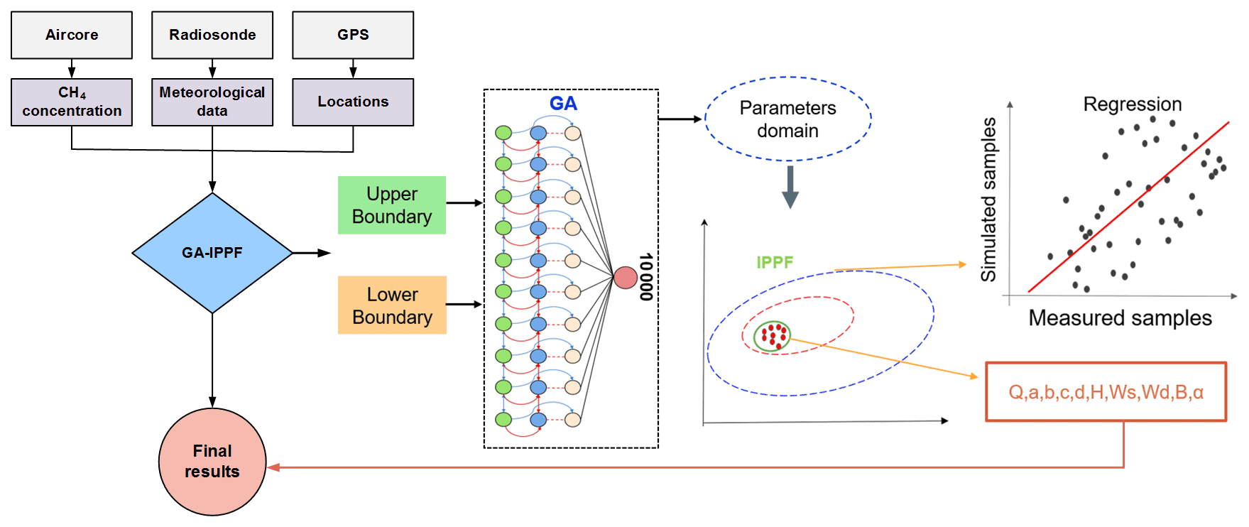
Therefore, we develop herein a model to overcome these shortcomings, named GA-IPPF, which combines the advantages of the genetic algorithm (GA) and an interior point penalty function (IPPF). The GA can model the fitness function as a process of biological evolution (Yuan and Qian, 2010), which can be used to calculate the potential solutions in a Gaussian dispersion model. IPPFs can find the minimum of the criteria in setting a domain (Kuhlmann and Buskens, 2018), which can help us achieve global optimal solutions for concerned parameters. Finally, GA-IPPF can calculate the diffusion parameters without prior information and reduce the impact of meteorological data on the calculated CH₄-emission rate.

We introduce the structure of our developed GA-IPPF in detail in Sect. 2. In Sect. 3, we evaluate the performance of GA-IPPF in a field campaign around a coal mine ventilation shaft by using the AirCore system on eight flights. Then, we discuss the comparisons between different quantification methods for CH₄ emission and evaluate the performance of GA-IPPF when the meteorological data are acquired from the fifth generation of European Centre for Medium-Range Weather Forecasts (ECMWF) atmospheric reanalysis of the global climate (ERA5) database. In Sect. 4, we validate the accuracy of GA-IPPF in observing system simulation experiments (OSSEs) and evaluate the uncertainty in the retrieved emission rate of CH₄. Furthermore, we test the performance of GA-IPPF in quantifying the emission rate based on three gas control release databases.

2 Data and methods

2.1 Active AirCore system

The active AirCore system comprises a ∼ 50 m coiled stainless-steel tube that works in conjunction with a micropump and a small pinhole orifice (45 µm) to sample air along the trajectory of a drone. If the pressure downstream of the orifice is more than half of that of the upstream (ambient) pressure, a critical flow through the orifice is obtained. This means that the flow rate depends only on two variables, namely, the air temperature and the upstream (ambient) pressure, both of which are monitored during the flight. After obtaining air samples during field campaigns, CO₂, CH₄, and CO collected by the AirCore system would be analyzed by a ground-based cavity ring-down spectrometer model, G2401-m (Picarro). For CH₄, the accuracy of samples is ±0.02 parts per million (ppm). The active AirCore system is controlled using an Arduino-built data logger, which records the temperature inside the carbon fiber housing. It also records the ambient temperature, ambient pressure, relative humidity, and pressure downstream of the pinhole orifice to ensure that critical flow is achieved. The data logger also logs the GPS coordinates. The weight of the active AirCore system is ∼ 1 kg. The active AirCore system is attached to a DJI Inspire Pro 1, which is capable of providing flights of ∼ 12 min.

2.2 Meteorological measurements

A radiosonde (Sparv Embedded AB, Sweden, model S1H2-R) measures ambient temperature, ambient pressure, ambient relative humidity, wind speed, and wind direction. The detection range of the temperature sensor is −40–+80 ^∘C, with an accuracy of 0.3^∘. The pressure sensor has a detection range of 300–1100 mbar, with an accuracy of 1 mbar. The relative humidity sensor measures in the range of 0 %–100 %, with an accuracy of approximately 2 %. Owing to the good connection between the radiosonde and satellites, we assume that the uncertainty in the wind direction is low. The wind speed can be estimated within a range of 0–150 m s⁻¹, with an uncertainty of approximately 5 %. If the wind-speed reading is less than 4 m s⁻¹, a minimum uncertainty of 0.2 m s⁻¹ is given. The radiosonde is lifted by a ∼ 30 L helium-filled balloon and is tethered onto a fishing line for easier retrieval after making a vertical profile.

2.3 Measurement site

The Pniówek coal mine (49.975^∘ N, 18.735^∘ E) is a large mine in Pniówek, Silesian Voivodeship, Poland, which is 190 km southwest of the capital Warsaw; see Fig. 1. It has a large coal reserve estimated to be about 101.3 million tons, and coal production is about 5.16 million tons per year.

Figure 1 Pniówek coal mine. (a) Red marks represent the location of Pniówek coal mine in Poland. (b) The surrounding area of Pniówek coal mine; blue marks represent Pniówek coal mine. (c) Detailed layout of Pniówek coal mine; deep mine with shaft.

2.4 Emission retrieval model

2.4.1 Gaussian dispersion model

The Gaussian dispersion model was used to analyze the CH₄ fugitive from the coal mine in this work. The location of an emission source is regarded as the coordinate origin; the x axis is the direction of the downwind, the y axis is the cross-wind direction, and the z axis is the altitude above the ground. Based on the established coordinate system, the Gaussian plume can be modeled by Eq. (1):

$$\begin{array}{}\text{(1)}& {\displaystyle }\begin{array}{rl}& C(x,y,z)={\displaystyle \frac{q}{\mathrm{2}\mathit{\pi }u{\mathit{\sigma }}_y{\mathit{\sigma }}_z}}\exp \left({\displaystyle \frac{-(y{)}^{\mathrm{2}}}{\mathrm{2}{\mathit{\sigma }}_y^{\mathrm{2}}}}\right)\\ & \left\{\exp \left({\displaystyle \frac{-(z-H{)}^{\mathrm{2}}}{\mathrm{2}{\mathit{\sigma }}_z^{\mathrm{2}}}}\right)+\mathit{\alpha }\cdot \exp \left({\displaystyle \frac{-(z+H{)}^{\mathrm{2}}}{\mathrm{2}{\mathit{\sigma }}_z^{\mathrm{2}}}}\right)\right\}+B,\end{array}\text{(2)}& {\displaystyle }{\mathit{\sigma }}_y=a\cdot x^b,\text{(3)}& {\displaystyle }{\mathit{\sigma }}_z=c\cdot x^d,\end{array}$$

where C is the concentration of CH₄ (g m⁻³), q (g s⁻¹) is the emission rate of CH₄ from the coal mine, u is the mean wind speed around the stack (m s⁻¹), H is the effective stack height, σ_y is the dispersion coefficient in the horizontal direction, σ_z is the dispersion coefficient in the vertical direction, u is the wind speed (m s⁻¹), and B is the background concentration of CH₄. Moreover, α is the reflection index of the measurement phenomenon, and x, y, and z are the positions of the samples in the determined coordinate system.

2.4.2 GA-IPPF model

First, the GA kernel calculates Q and other dispersion parameters with a first guess (Liu and Michalski, 2016). It guarantees that the unknown parameters are retrieved through the global optimum solution, as shown in Fig. 2. Then, the results calculated by the GA serve as initial input parameters and constraints in the IPPF model, and actual values of the concerned parameters are retrieved by IPPF. Detailed information can be found in Sect. S1 (Supplement).

Based on the Gaussian dispersion model, auxiliary meteorological data, location information, and CH₄ samples, we determine the unknown parameters in Eqs. (1) to (3) by using GA, including q, H, a, b, c, d, and α, in a logical range constrained by the lower boundary and upper boundary. First, the locations and concentrations of CH₄ samples and wind serve as the initial input of Eq. (1). Then, the fitness value evaluates the applicability of the calculated parameters in each step. We define the fitness value as

$$\begin{array}{}\text{(4)}& {\displaystyle }F=\sum _{i=\mathrm{1}}^n(C_{\mathrm{m}}^i-C_{\mathrm{s}}^i{)}^{\mathrm{2}},\text{(5)}& {\displaystyle }\begin{array}{rl}& C_{\mathrm{s}}^i(x,y,z)=\sum _{i=\mathrm{1}}^n{\displaystyle \frac{q^{\prime }}{\mathrm{2}\mathit{\pi }{u}^{\prime }{\mathit{\sigma }}_y^{\prime }{\mathit{\sigma }}_z^{\prime }}}\exp \left({\displaystyle \frac{-(y{)}^{\mathrm{2}}}{({\mathit{\sigma }}_y^{\prime }{)}^{\mathrm{2}}}}\right)\\ & \mathit{\{}\exp \left({\displaystyle \frac{-{\left(z-H^{\prime }\right)}^{\mathrm{2}}}{{\left({\mathit{\sigma }}_z^{\prime }\right)}^{\mathrm{2}}}}\right)+{\mathit{\alpha }}^{\prime }\cdot \exp \left({\displaystyle \frac{-(z+H^{\prime }{)}^{\mathrm{2}}}{({\mathit{\sigma }}_z^{\prime }{)}^{\mathrm{2}}}}r\right)\mathit{\}}\\ & +B^{\prime },\end{array}\end{array}$$

where F is the fitness value, n is the total number of concentration samples, $C_{\mathrm{m}}^i$ is the sample CH₄ concentration, i is the number of samples, $C_{\mathrm{s}}^i$ is the simulated concentration of CH₄ in the location of samples calculated by Eq. (5), and q^′, u^′, σ_y, σ_z, H^′, α^′, and B^′ are the calculated CH₄-emission rate, wind speed, diffusion parameters, emission height, reflection index, and background CH₄ concentration, respectively, acquired from the “Mutation” in Fig. 2. When f is less than the threshold value ($\mathrm{1}\times {\mathrm{10}}^{-\mathrm{5}}$) of the fitness value, the corresponding parameters are treated as the results of output.

IPPF rebuilds the inequality constraint conditions to the unconstrained solution process. It forces the start point to satisfy the constraints, as shown in Eq. (6).

$$\begin{array}{}\text{(6)}& minF\left(x,r_k\right)=f\left(x\right)+r_{k}B\left(x\right),\end{array}$$

where f(x) is the unconstrained equation, and r_k is the coefficient of the constrained equation B(x). When the solution parameters are out of the constraints, r_kB(x) is large, thereby ensuring that the final solution is feasible under the inequality constraint conditions.

To obtain the inequality constraints, the GA is repeated 10 000 times, and the mean values of the calculated wind speed, wind direction, H, a, b, c, d, and α are treated as the initial input of the IPPF model. The domains of H, a, b, c, d, and α are determined by 2 times the standard deviation of the corresponding results in the GA. The constraint values of wind speed (W_s) and direction (W_d) are set according to the precision of actual measurements, m±σ, whereas m is the measured value of wind speed or wind direction, and σ is their measured precision. Actual B values are considered to be within 1800–2500 ppb. Then, the Pearson correlation coefficient (R) values of the actual samples and simulated values work as the criteria in the solution process of Eq. (7).

$$\begin{array}{}\text{(7)}& R={\displaystyle \frac{{\sum }_{i=\mathrm{1}}^n\left(C_{\mathrm{s}}^i-\stackrel{\mathrm{‾}}{C_{\mathrm{s}}}\right)\left(C_{\mathrm{m}}^i-\stackrel{\mathrm{‾}}{C_{\mathrm{m}}}\right)}{\sqrt{{\sum }_{i=\mathrm{1}}^n{\left(C_{\mathrm{s}}^i-\stackrel{\mathrm{‾}}{C_{\mathrm{s}}}\right)}^{\mathrm{2}}}\sqrt{{\sum }_{i=\mathrm{1}}^n{\left(C_{\mathrm{m}}^i-\stackrel{\mathrm{‾}}{C_{\mathrm{m}}}\right)}^{\mathrm{2}}}}}\end{array}$$

The results are treated as the final retrieved values of the concerned parameters when R reaches the maximum.

Figure 2 Flow chart of the GA-IPPF model, including data inputs and processes in each step.

2.4.3 Uncertainty analyses

The GA-IPPF model will be calculated 1000 times repeatedly based on the collected samples of CH₄ concentrations; then, the uncertainty and final retrieved emission rate could be defined by

$$\begin{array}{}\text{(8)}& {\displaystyle }\mathit{\sigma }=\sqrt{{\displaystyle \frac{\sum _{i=\mathrm{1}}^N(q_i-\stackrel{\mathrm{‾}}{q}{)}^{\mathrm{2}}}{N}}},\text{(9)}& {\displaystyle }{q}_{\mathrm{r}}=\stackrel{\mathrm{‾}}{q}={\displaystyle \frac{\mathrm{1}}{N}}\sum _{i=\mathrm{1}}^N{q}_i.\end{array}$$

σ is the uncertainty of the retrieved emission rate, q_i is the ith retrieved emission rate, $i=\mathrm{1},\mathrm{2},\mathrm{3}\mathrm{\dots }\mathrm{1000}$, $\stackrel{\mathrm{‾}}{q}$ is the mean value of q_i, N is 1000, and q_r is regarded as the value of the retrieved emission rate. The values of other parameters ($a,b,c,d,H,W_{\mathrm{s}},W_{\mathrm{d}},B,\mathit{\alpha }$) calculated by GA-IPPF are also defined according to the same principle.

3 Results

3.1 Actual experiments

As part of the Carbon Dioxide and Methane Mission (CoMet) pre-campaign, 15 active AirCore flights successfully collected data around a ventilation shaft of Pniówek coal mine on 18 and 21 August 2017. The sample data on Flight 6 (18 August 2017) and Flight 15 (21 August 2017) were used to evaluate the GA-IPPF model in detail, as shown in Fig. 3. Retrieved results of data collected by other flights are presented in Sect. S2 (Supplement).

Figure 3 Samples of CH₄ concentrations on two flights: (a) Flight 6 and (b) Flight 15.

On Flight 6, the AirCore system collected CH₄ from 0 to 98 m around the ventilation shaft in a spiral pattern, with a total of 376 samples, ranging from 1980.1 to 49 113.9 ppb, and a measurement period of 7 min. On Flight 15, the AirCore system collected CH₄ with a total of 400 samples, ranging from 2131.7 to 57 265.3 ppb, and a measurement period of 9 min. Both flights show high spatial variability in CH₄ exhaust from the ventilation shaft. Subsequently, we inputted the wind speed, wind direction, location information, and CH₄ samples collected from flights into the GA-IPPF model. To express the final retrieved emission (Q) (g s⁻¹), the dry-air mixing ratio of CH₄ (ppb) is transformed into mass concentration m (mg m⁻³) as follows:

$$\begin{array}{}\text{(10)}& m=C\cdot {\displaystyle \frac{M_{{\mathrm{CH}}_{\mathrm{4}}}}{M_{\mathrm{Air}}}}\times {\mathrm{10}}^{-\mathrm{3}},\end{array}$$

where $M_{{\mathrm{CH}}_{\mathrm{4}}}$ is the molar mass of CH₄, and M_air is the molar mass of air.

The retrieved results are shown in Table 1, and the uncertainty is presented in the discussion in detail. Notably, the emission height on Flight 15 was larger than that of Flight 6, which might be caused by the difference in thermal energy and vertical wind speed of the two flights. The background concentrations of CH₄ were 1.43 and 1.41 mg m⁻³ on Flights 6 and 15, respectively, which show little difference. The dates of the two flights were very close, so the background concentration of CH₄ in 2 d had nearly the same seasonal characteristics. The exhaust gases of the coal mine were emitted through the ventilation shaft with effective emission heights of 58.4 and 35.5 m, respectively.

To evaluate the rationality of the retrieved results, these parameters are used to simulate CH₄ diffusion from the ventilation shaft according to Eq. (1). The comparison between simulated CH₄ concentration data and actual samples in the same locations is shown in Fig. 4.

Table 1 Results calculated by the GA-IPPF model.

Then, we also calculate the difference between the actual measured samples and simulated ones as

$$\begin{array}{}\text{(11)}& D_{\mathrm{c}}=C_{\mathrm{s}}-C_{\mathrm{m}},\end{array}$$

where D_c is the difference in CH₄ concentration data between actual measured and simulated ones, C_s is the simulated CH₄ concentration (mg m⁻³), and C_m is the measured CH₄ concentration (mg m⁻³).

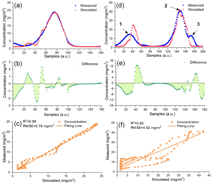
Figure 4 Comparison between the measured samples and the simulated ones based on the parameters in Table 1: (a) Flight 6 and (d) Flight 15. The difference in simulated CH₄ concentration data and actual measured ones: (b) Flight 6 and (e) Flight 15. Correlation analysis: (c) Flight 6 and (f) Flight 15.

Figure 4 shows that the simulated CH₄ concentration is very consistent with actual sampled ones on two flights. On Flight 6, the largest value of the sampled CH₄ concentration is 23.92 mg m⁻³, while the corresponding simulated one is 22.45 mg m⁻³, and the relative error is only 0.2 %. It is worth noting that there exist three peaks on Flight 15, mainly occurring at the altitudes of about 16, 25 and 40 m; see Sect. S3 in the Supplement. Figure 4d shows that the simulated CH₄ concentration data around the first and third peaks are not better than those around the second peak, because the GA-IPPF method can assign more weights to the samples with higher concentrations (nos. 120 to 180 on Flight 15) to get the global optimal solution of the unknown parameters, which leads to lower fitness in the simulated CH₄ concentration around the first and third peaks. Values of D_c range from −2.50 to 2.35 mg m⁻³ on Flight 6, which are lower than that on Flight 15. R² values between the simulated CH₄ concentration and actual sampled ones are larger than 0.8 on two flights, and root mean square errors (RMSEs) are 0.79 and 4.52 mg m⁻³, respectively. The simulated CH₄ concentrations on the other flights are seen in Sect. S2. In summary, the tendency of the simulated CH₄ concentration data remains consistent with that of the actual samples on the flights.

3.2 Comparison with other methods

To investigate the difference between our proposed emission model and the others, three methods were applied to estimate CH₄ emissions on all the flights, including a mass-balance approach, nonlinear least square fit (NLSF), and facility emission.

The mass-balance approach quantifies CH₄ emissions by calculating the cross-sectional flux perpendicular to the wind direction (Krings et al., 2018). First, a two-dimensional plane is selected according to the number of CH₄ samples. Second, the two-dimensional plane is divided into a grid of equal spatial resolution. Third, CH₄ samples are regarded as original points to interpolate full grids defined by the kriging interpolation scheme (Mays et al., 2009). Finally, the emission rate of the CH₄ source is calculated by

$$\begin{array}{}\text{(12)}& F_{\left({\mathrm{CH}}_{\mathrm{4}}\right)}=\int \int v\sin \left(\mathit{\alpha }\right)\cdot (C_{(x,z)}-C_{\mathrm{bg}})\mathrm{d}x\mathrm{d}z,\end{array}$$

where v is the wind speed, α is the angle between wind direction and the two-dimensional plane, C_(x,z) is the density of CH₄ in each grid, and C_bg is the background of CH₄ in each grid. The uncertainty analyses of this method are detailed in Nathan et al. (2015).

NLSF and the combination of NLSF with the Gaussian diffusion model are also extensively used for point-source emission retrieval (Zheng et al., 2020; Wolff et al., 2021). In this study, NLSF is used to estimate Q on each flight by fitting the unknown parameters in Eq. (1).

Andersen et al. (2021) also developed an inverse Gaussian approach to quantify CH₄ emissions from coal mine ventilation shafts based on the same flights. Firstly, the Gaussian dispersion is built as

$$\begin{array}{}\text{(13)}& \begin{array}{rl}C(x,y,z)& ={\displaystyle \frac{q}{\mathrm{2}\mathit{\pi }u{\mathit{\sigma }}_y{\mathit{\sigma }}_z\cos \left(\mathit{\theta }\right)}}\exp \left({\displaystyle \frac{-(y{)}^{\mathrm{2}}}{\mathrm{2}{\mathit{\sigma }}_y^{\mathrm{2}}}}\right)\\ & \left\{\exp \left({\displaystyle \frac{-(z-H{)}^{\mathrm{2}}}{\mathrm{2}{\mathit{\sigma }}_z^{\mathrm{2}}}}\right)+\exp \left({\displaystyle \frac{-(z+H{)}^{\mathrm{2}}}{\mathrm{2}{\mathit{\sigma }}_z^{\mathrm{2}}}}\right)\right\},\end{array}\end{array}$$

where θ is the angle between the wind direction and the perpendicular line of the flight trajectory. This model does not include the item of the background of CH₄. Furthermore, σ_y and σ_z are treated as certain values in Eq. (11).

Facility-emission data and hourly CH₄ emission from the shaft are calculated by measuring raw CH₄ concentration and air flux through the shafts, following the equation below:

$$\begin{array}{}\text{(14)}& Q_{\mathrm{inventory}}={\displaystyle \frac{P\cdot V_{\mathrm{flow}}}{R\cdot T}}\mathit{\rho },\end{array}$$

where V_flow is the volumetric flow rate of CH₄ (m³ s⁻¹), given by the air flow rate (scaled by a constant factor of 0.95 to account for the ∼ 5 % additional air flow not coming from the ventilation shaft) multiplied by the CH₄ concentration, and P, R, T, and ρ are the atmospheric pressure (Pa), the universal gas constant (J mol⁻¹ K⁻¹), the ambient temperature (K), and the molar density of CH₄ (g mol⁻¹) (16.043 g mol⁻¹), respectively.

CH₄-emission rates from ventilation shafts estimated by hourly facility-emission data for 18 and 21 August 2017 are 1655.3 ± 479.45 and 913.2 ± 285.4 kg h⁻¹, respectively, as shown in Fig. 5.

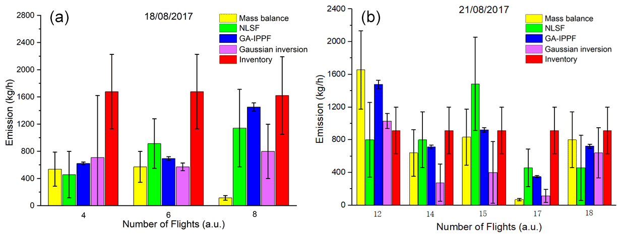
Figure 5 Quantified CH₄ emission by different methods based on the collected data: (a) 18 August 2017 and (b) 21 August 2017. CH₄-emission rates from ventilation shafts calculated by mass balance and inverse Gaussian refer to Andersen et al. (2021).

As shown in Fig. 5, Flights 4, 6, and 8 were measured on 18 August 2017, whereas Flights 12, 14, 15, 17, and 18 were measured on 21 August 2017. Figure 5a shows that the CH₄-emission rates calculated by mass balance are smaller than the inventory estimation on all of the flights. On Flight 8, q retrieved by mass balance is far lower than those quantified by the other methods, whereas q retrieved by the GA-IPPF model (1478.4 ± 50.3 kg h⁻¹) shows only a slight difference from the inventory. As shown in Fig. 5b, CH₄ emissions retrieved by the mass-balance, inverse Gaussian, and GA-IPPF models are overestimated compared with the inventory on Flight 12. The mass-balance and inverse Gaussian methods also show an obviously underestimated q on Flight 17. Estimations of retrieved CH₄ emissions on Flight 18 show consistency among the methods of mass balance, GA-IPPF, and inverse Gaussian. The CH₄-emission rate of coal generally has significant variability in each measurement, even on the same day. Mass balance is very sensitive to the size settings of grids, and both height and length settings can affect the concentration distribution across the cross section. NLSF has a high-accuracy requirement for wind measurements, and errors in these measurements have a linear influence on the final emission estimation. Notably, the standard errors of q quantified by GA-IPPF are always the lowest among these methods, indicating the stability of the model we developed, and we also simulated a 2-D CH₄ plume from the ventilation shaft on Flight 6 and Flight 15 based on different methods, as seen in Sect. S4.

3.3 Application of the reanalysis meteorological database in the GA-IPPF model

Wind speed and wind direction acquired by the radiosonde or weather station are the two main parameters in GA-IPPF. However, additional sensors are bound to increase the cost and difficulty during actual CH₄-emission measurements. To explore the possibility of weather reanalysis data instead of actual wind measurement by sensors, we use 10 m U and V wind components from the ERA5 meteorological reanalysis database (spatial resolution is 0.1^∘ × 0.1^∘, and temporal resolution is 1 h) developed by the ECMWF (Hersbach et al., 2020) to evaluate the GA-IPPF model. However, the wind directions from ERA obviously differed from the actual measurements during the flights. Hence, we determine the wind direction by using the CH₄ samples; for example, the line between the shaft and the location of the maximum values of samples at the same heights was treated as the downwind direction, whose uncertainty was set to 50^∘. Wind speed from ERA is used for the CH₄-emission calculation, and the uncertainty was supposed to be 2 m s⁻¹. Even if the initial wind speed and wind direction obviously differed between the two sources, the GA-IPPF model adjusted them into reasonable ranges. The results of q retrieved by two meteorological data sources during all flights were evaluated, as shown in Table 2.

Table 2 CH₄ emission retrieved by two meteorological data sources.

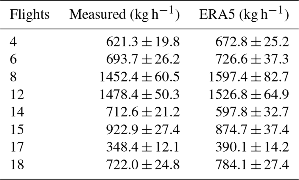
Table 2 shows that the values of quantified q between the two meteorological sources are within 20 % on the same flight. The standard errors of q retrieved by the ERA5 database are larger than those from actual measurements, wind data acquired from the ERA5 database perhaps being treated as alternative input parameters in the GA-IPPF model if no meteorological instruments are equipped in field experiments. We also explore the reason for little difference in the calculated emission rates by the two different sources of meteorological data. The concerned parameters on Flight 6 and Flight 15 calculated based on ERA5 meteorological data are presented in Table 3.

Table 3 Parameters retrieved by GA-IPPF through the ERA5 database.

The initial wind speed and wind direction in Table 3 are obviously different from those in Table 1. However, the retrieved wind directions are nearly the same based on the two sources of meteorological data. Retrieved diffusion parameters and emission heights also show less difference in two tables (Tables 1 and 3). It is worth noting that the wind speed and reflection index can be adjusted to reach the global solution by the GA-IPPF model, which leads to little bias in retrieving the emission rate.

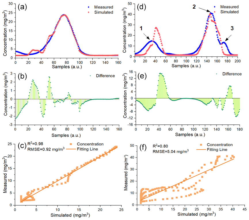
Figure 6 Comparison between the measured samples and the simulated ones based on the ERA5 meteorological data: (a) Flight 6 and (d) Flight 15. The difference between simulated CH₄ concentration data and actual measured ones: (b) Flight 6 and (e) Flight 15. Correlation analysis: (c) Flight 6 and (f) Flight 15.

The tendencies of simulated CH₄ concentration data on the two flights are similar to that in Fig. 4. What is more, both R² and RMSE between simulated CH₄ concentration data and actual measured ones on both flights show less difference with that in Fig. 4. Values of D_c shown in Fig. 6b range from −2.25 to 2.62 mg m⁻³, which is nearly the same as the result in Fig. 4b. Values of D_c shown in Fig. 6e range from −11.04 to 15.21 mg m⁻³ and from −11.3 to 12.85 mg m⁻³ in Fig. 4e. The difference between the actual measured wind speed and the ERA5 speed is 0.8 m s⁻¹ on Flight 15, which is larger than that on Flight 6 (0.3 m s⁻¹). In summary, GA-IPPF can still simulate reasonable diffusion of CH₄ through ERA5 wind data.

4 Discussion

4.1 Validation of the performance of the GA-IPPF model through OSSEs

Firstly, the dispersion of CH₄ emission from a strong point source was simulated by Eq. (1) using the dispersion parameters shown in Table 4. To make the simulations close to the actual measurement scenarios, random errors were added to the CH₄ concentration samples (0.5 %), wind speed (±0.3 m s⁻¹), and wind direction (±20^∘). Then, the simulated flight track of the UAV was conducted in the cross section (300 m to a strong source) in Fig. 7. The spatial resolution of the supposed samples is set to 10 m, and 99 samples are selected from the simulated dispersion to represent the data acquired by the UAV-based AirCore. Then, the concerned parameters are retrieved by the GA-IPPF method based on the above assumptions. Simulations are repeated 10 000 times, and the average values of the corresponding parameters were treated as the “Retrieved” results in Table 4.

Figure 7 Rectangle represents the transect perpendicular to the wind direction, covering a distance of 300 m near the point source. Red line represents the simulated flight track of the UAV-based AirCore system. Colored points represent the CH₄ concentration samples in OSSEs (99 in total).

Table 4 The parameter settings in the dispersion simulation and the retrieved results by GA-IPPF.

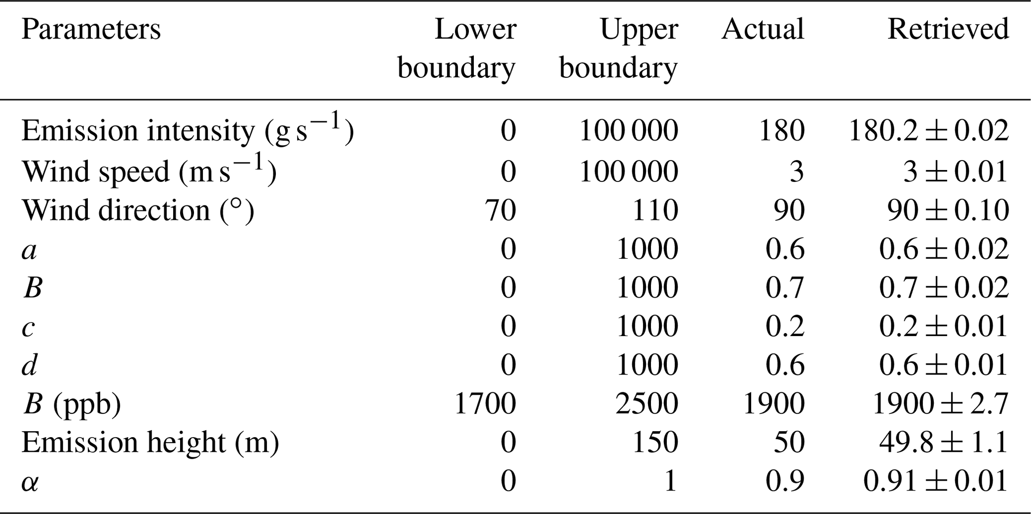
“Actual” means the set values of parameters, and “Retrieved” means the average values of parameters retrieved by the GA-IPPF model through 10 000 times of simulation.

As shown in Table 1, q retrieved by GA-IPPF has only a 0.11 % bias compared with the set values. Emission height only has 0.2 m bias in terms of the set one, and the uncertainty is only 0.4 % to 50 m. Other retrieved parameters also show high consistency with the original settings.

4.2 Stability analyses

The necessary input parameters in GA-IPPF contain the meteorological data (wind speed and wind direction), accuracy of CH₄ samples, and number of CH₄ samples. In Eq. (1), wind speed has a nearly linear relationship with the emission estimation. Wind speed is also an important factor that determines atmospheric stability according to the Pasquill–Gifford method (Venkatram, 1996) as it affects the diffusion parameters of σ_y and σ_z. The coordinate is built according to the wind direction, which is defined as the plane coordinates of CH₄ samples. According to Eqs. (2) to (3), errors in wind-direction measurement led to wrong σ_y and σ_z in each position of the samples. CH₄ samples are the most important factors in determining the Gaussian diffusion. The accuracy of samples influences the judgment of “fitness” in the GA process. More samples collected in different positions help rebuild the spatial-distribution characteristics of the plume, because this provides a larger possibility for the fitting process in IPPF and helps determine the optimum solution. To evaluate the influence of errors in the measurements of necessary parameters on the final retrieved results, the same settings in Table 4 are used as actual results. The performance of the GA-IPPF model with additional random errors in each parameter was simulated 10 000 times, as shown in Fig. 8.

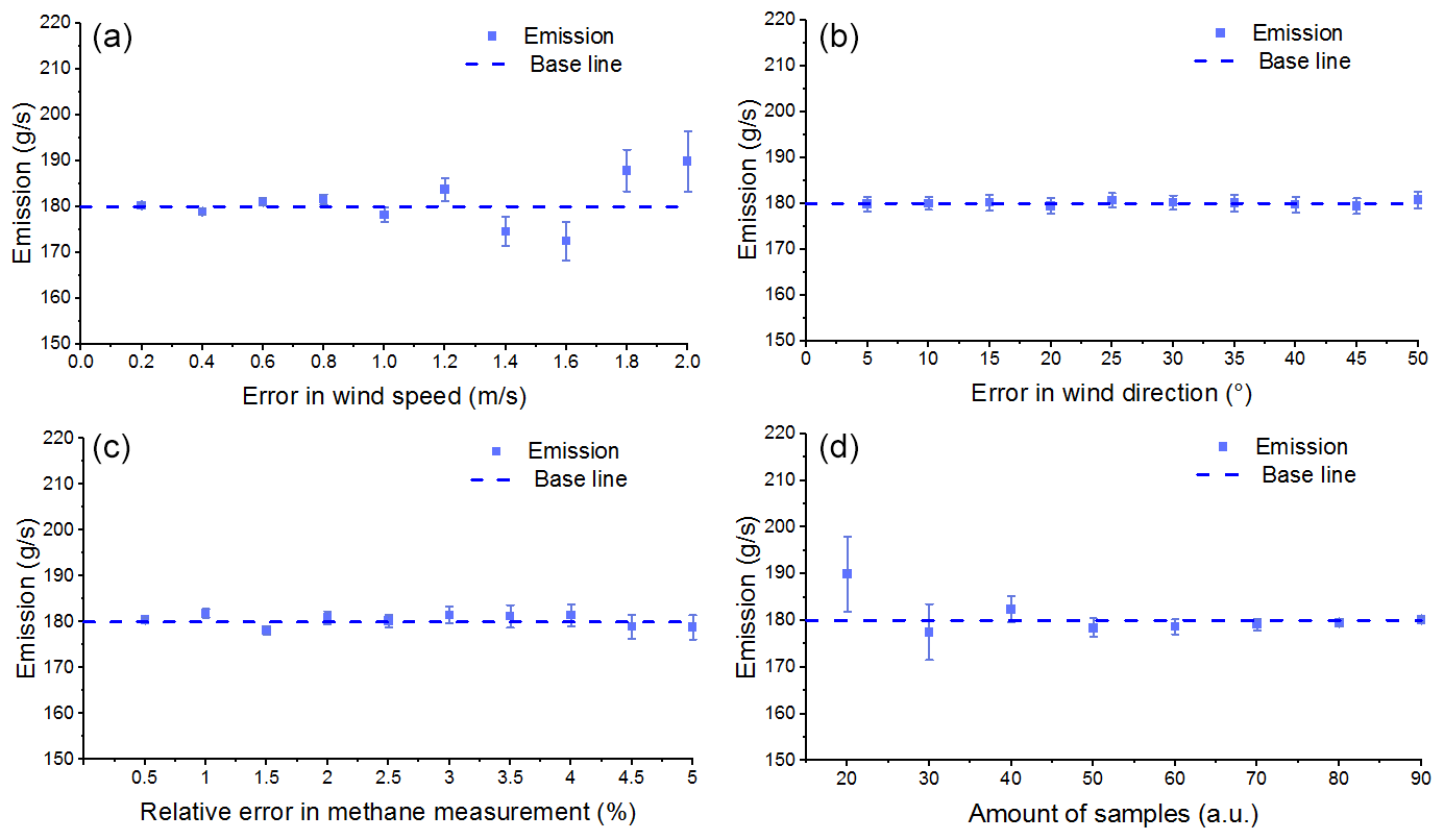
Figure 8 Influence of accuracy of parameters on retrieved emission results. The baseline represents the emission rate setting of CH₄, 300 g s⁻¹: (a) wind speed, with additional error ranging within 0.2–2 m s⁻¹ and an interval of 0.1 m s⁻¹, (b) wind direction, with additional error ranging within 5–50^∘ and an interval of 5^∘, (c) accuracy of CH₄ samples, with additional error ranging within 0.5 %–5.0 % and an interval of 0.5 %, and (d) number of CH₄ samples, randomly selected as 20–90 among the defined 99 samples.

In Fig. 8a, the mean value of q retrieved by GA-IPPF is nearly the same as the baseline if the error in wind speed is less than 0.4 m s⁻¹. It occurs in the maximum retrieved emission bias (10.2 g s⁻¹) to the baseline with a 2 m s⁻¹ error in wind speed. Fluctuation of q occurs obviously if the error in wind speed exceeds 0.4 m s⁻¹. The standard errors of q are positively correlated with the values of errors in wind speed, indicating that the accuracy of wind speed measurements largely influences the stability of the GA-IPPF model. This model has a self-adjustment function for wind speed; for example, when the initial wind speed is 3 m s⁻¹, the maximum standard error of q is only 6.6 g s⁻¹ (3.7 % to 180.0 g s⁻¹) when the additional error in wind is 2.0 m s⁻¹ (66.7 % to 3.0 m s⁻¹).

The retrieved q shows less sensitivity to errors in wind direction (see Fig. 8b). When errors in wind direction are 5 to 40^∘, all biases of q are within 0.7 g s⁻¹, and the standard errors are around 1.6 g s⁻¹. Wind direction determines the spatial location of the sampling point, and wrong location information leads to distinct errors in emission estimation. GA-IPPF shows a highly accurate ability to obtain the global optimum solution in wind direction.

Sampling accuracy has a small impact on the retrieved q within different settings in CH₄ sample accuracy; see Fig. 8c. Standard deviation is positively correlated with errors in CH₄ measurements. The standard deviation is 2.6 g s⁻¹ when the measurement error reaches 5.0 %. Notably, the uncertainty of CH₄ samples measured by the UAV-based AirCore system is far less than 5.0 %. The UAV-based AirCore system can acquire more than 99 CH₄ samples in actual feasible measurements; therefore, it is believed that the accuracy of CH₄ samples (> 95.0 %) collected by the AirCore system brings less influence in theory.

The number of measurement points obviously influences the final accuracy of q by the GA-IPPF model (see Fig. 8d). It has a bias of 9.7 to 180.0 g s⁻¹ when n is 20. The accuracy of q and the standard error are negatively correlated with n, which provides the number of criteria for the fitting process in the retrieval model. Hence, n directly influences the retrieved results. The AirCore system has the advantage of continuous sampling during flight, which integrates the atmospheric signals along the flight path and helps reduce the uncertainty in the retrieved q. Besides, the smoothing of the atmospheric signal also reduces the spatial resolution of the measurements, which needs to be considered during the optimization.

IPPF can suitably solve the problem of inequality constraints, and the calculated solution guarantees the calculated parameters will be within the feasible region. In this section, the performance of the GA-IPPF model and the influence of the four key input parameters are discussed.

4.3 Suggestions for quantifying emission rates through the UAV-based AirCore system

1. Meteorological instruments should be equipped when collecting concentration samples to acquire wind speed, wind direction, humidity, and atmosphere pressure.

2. The wind speed should be greater than 2.0 m s⁻¹.

3. During actual experiments, after the stable wind speed and wind direction are measured, the UAV-based AirCore system will start its concentration collection, and the system should try to fly along the cross section perpendicular to the wind direction.

These criteria were used to select the analyzed 8 flights from the total of 15 flights.

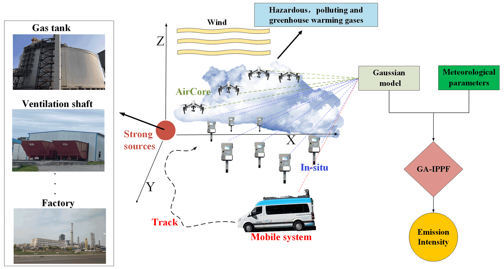
Figure 9 Application of GA-IPPF in quantifying emission sources of gases through different sample systems, including the UAV-based AirCore system, ground-based in situ network, and mobile collection system.

4.4 Application of GA-IPPF

GA-IPPF works as an emission gas quantification method, which can achieve rapid real-time monitoring of methane leakage caused by landfills, chemical plants, and other strong sources. In theory, the recommended model is applicable not only to the UAV-based AirCore system, but also to other sample systems which can measure gas concentration and location information. Each country's environmental monitoring department may have built gas sample equipment based on different platforms, including the UAV, vehicles, and ground-based in situ stations. These systems may monitor greenhouse gases like CO₂ and CH₄ as well as polluting and harmful gases. Therefore, we demonstrate the application of GA-IPPF in quantifying gas emissions based on different gas concentration measurement systems in actual experiments.

4.5 Emission estimates in control release experiments

To evaluate the performance of GA-IPPF in control release experiments, we quantify the gas emission rates in release experiments through different gas sample systems, including the UAV-based AirCore system, mobile sampling system, and ground-based in situ network. A detailed introduction of the concerned release experiment is as follows.

4.6 Agrar Hauser control release

This CH₄ release experiment was conducted on Agrar Hauser field near Dübendorf, Switzerland (Morales et al., 2022). The controlled CH₄ was released from an artificial-source 50 L high-pressure cylinder with a height of 1.5 m. Meteorological information was acquired by 3-D anemometers around the emission source. UAV-based sample systems used in these release experiments contained two sensors, a quantum cascade laser spectrometer (QCLAS) and the active AirCore. The release experiments were performed from 23 February to 14 March 2020. There was no other CH₄ source around Agrar Hauser field, and the topography was flat. In this section, active AirCore CH₄ samples on 12 March 2020 (312_01) were chosen to use GA-IPPF to quantify the methane release rate.

4.7 EPA methane control release

The Environmental Protection Agency (EPA), USA, developed the OTM 33A method to quantify oil and gas leakage based on mobile measurement platforms (Brantley et al., 2014), which consisted of a CH₄ in situ sensor (G1301-fc cavity ring-down spectrometer; Picarro), a co-located compact weather station, and a Hemisphere Crescent R100 Series GPS system. The accuracy of the in situ sample was within ±5 %, and the in situ sensor was implemented at a height of 2.7 m based on the vehicle. The weather station provided atmospheric temperature, pressure, and humidity as well as 3-D wind direction and wind speed. A 99.9 % CH₄ high-pressure cylinder was used as the gas supply to simulate the CH₄ leakage source. The EPA published a total of 20 experiments of control releases to evaluate the OTM 33A method.

Table 5 Performance of the GA-IPPF model in different control release experiments.

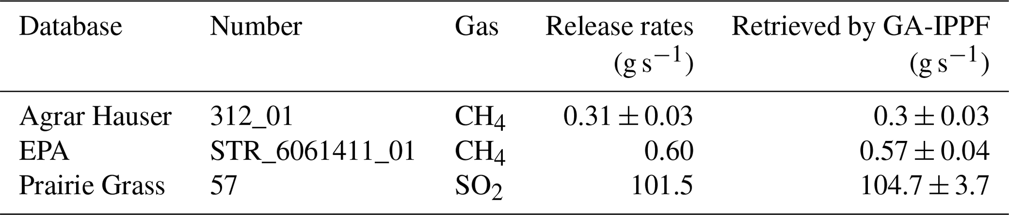
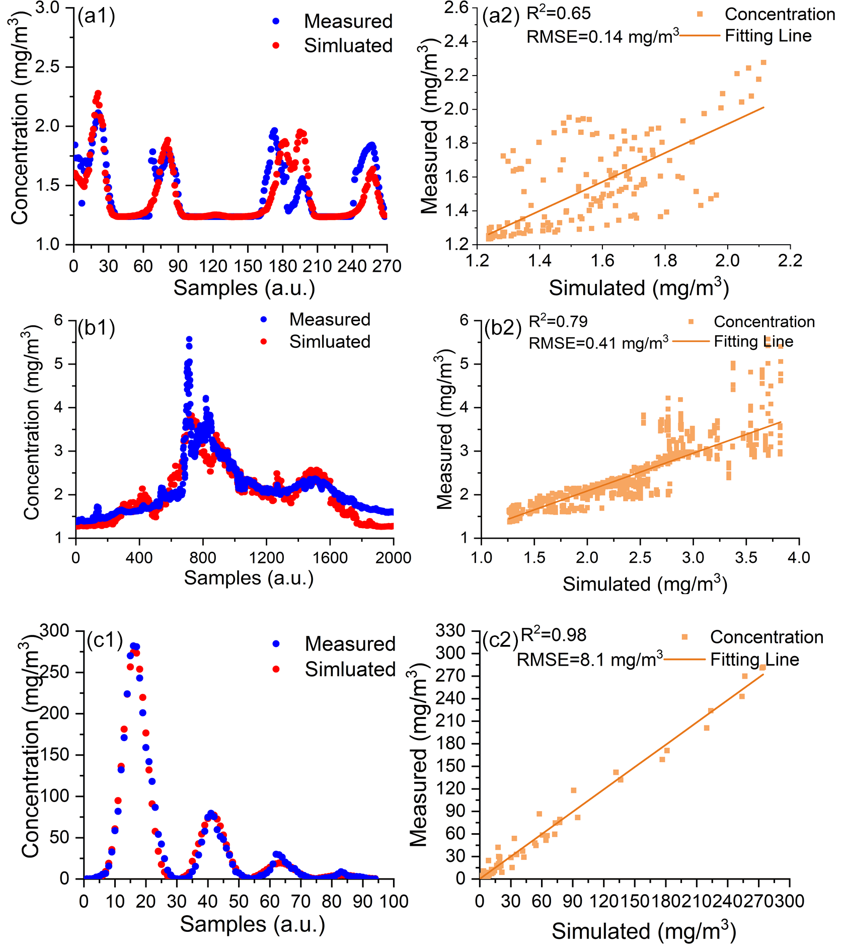
Figure 10 The simulated gas diffusions based on retrieved parameters in control release experiments. Panels (a1) and (a2) are comparisons between simulated diffusion and actual samples in Agrar Hauser. Panels (b1) and (b2) are comparisons between simulated diffusion and actual samples in the EPA control release. Panels (c1) and (c2) are comparisons between simulated diffusion and actual samples in the Prairie Grass experiment.

4.8 Prairie Grass emission experiment

The Prairie Grass emission experiment was mainly conducted to evaluate the diffusion of SO₂ from a point source under different meteorological conditions (Barad, 1958). The height of the emission source was 0.46, and all in situ sensors were set at a height of 1.5 m. SO₂ concentration was sampled by the in situ network at radii of 50, 100, 200, 400, and 800 m around the source. Samples in the R57 release (10 min sampling periods), totaling 94, were selected to quantify the SO₂ emission rate from the release instrument. The reported emission rate of SO₂ in R57 was 105.1 g s⁻¹, and the samples collected at the radius of 800 m were neglected in this discussion because of their very small quantity. The reported wind speed was 4.85 ± 1 m s⁻¹, and the wind direction was 184 ± 10^∘.

Table 4 shows the emission rates and uncertainties through GA-IPPF in control release experiments and the reported emission rates. The average difference between retrieved emission rates and reported ones is 3.8 %, which indicates the high accuracy of GA-IPPF in quantification estimation.

As shown in Fig. 10, the gas diffusions simulated by GA-IPPF in the three control release experiments conform to logic. Simulated gas concentrations are in good agreement with actual samples (see Fig. 10a1, b1, and c1,), and each peak of the samples in the control release experiments can be reconstructed. The correlations between simulated gas concentrations and actual samples are larger than 0.65, and the RMSEs are within 2.7 % (relative to the mean value of the selected samples' concentration).

In general, reconstructions of gas concentrations based on both mobile platforms and UAV are worse than that based on the in situ network. Collected data by the in situ network are usually the mean value of a certain time, like 10 min in the Prairie Grass emission experiment, which provides stable input data for GA-IPPF, especially concentration samples, while the concentrations sampled by the mobile-platform- and UAV-based AirCore experiments are instantaneous, which may not capture the temporal variability of emissions. The advantage of vehicle-based and UAV-based sample systems is flexibility; that is, they can freely acquire the distribution of gases around the target monitoring sources. In situ network implementation is complicated by a high cost, and the wind direction should be considered during deployment. However, its high stability and accuracy can help us to quantify the emission source. Therefore, environmental protection departments can choose detection systems according to actual emission monitoring needs.

5 Conclusions

In this study, we present a quantified model for a strong point emission source based on concentration sampling data, named GA-IPPF. During the CoMet campaign in 2017, we successfully monitor methane emissions from a ventilation shaft in Pniówek coal mine through the concentration data measured by the UAV-based AirCore system. Results show that CH₄-emission rates from ventilation shafts are not consistent even in a short time.

GA-IPPF can reconstruct the concentration dispersion around the point emission source, and the largest R² between the measured CH₄ concentration and the reconstructed concentration on the selected flights around Pniówek coal mine can reach 0.99.

In observing system simulation experiments (OSSEs), we discussed the sensitivity analysis of different parameter settings to the final retrieved emission rate by GA-IPPF. We demonstrate that GA-IPPF has a self-adjust function to achieve an optimal solution for the emission rate, which will reduce the requirements for hardware performance in the actual emission quantification experiment.

We also tested the performance of GA-IPPF in three control release experiments with different sampling platforms, including the vehicle-mounted in situ system, UAV-based AirCore system, and ground-based in situ network observation, and the biases between retrieved emission rates and reported ones are within 5.0 %.

In future, GA-IPPF has great potential in point-source quantification based on the mobile concentration sampling system, which can help to renew and enrich the gas emission inventories on strong point sources.