Significant enhancements of the mesospheric Na layer bottom below 75 km observed by a full-diurnal-cycle lidar at Beijing (40.41° N, 116.01° E), China

Based on the full-diurnal-cycle sodium (Na) lidar observations at Beijing (40.41^∘ N, 116.01^∘ E), we report pronounced downward extensions of the Na layer bottomside to below 75 km near mid-December 2014. Considerable Na atoms were observed even as low as ∼ 72 km, where Na atoms are short-lived. More interestingly, an unprecedented Na density of ∼ 2500 atoms cm⁻³ around 75 km was observed on 17 December 2014. Such high Na atoms concentration was 2 orders of magnitude larger than that normally observed at the similar altitude region. The variations of Na density on the layer bottom were found to be accompanied by warming temperature anomalies and considerable perturbations of minor chemical species (H, O, O₃) in the upper mesosphere. Different from the previous reported metal layer bottom enhancements mainly contributed by photolysis after sunrise, these observational results suggest more critical contributions were made by the Na neutral chemical reactions to the Na layer bottom extensions reported here. The time–longitudinal variations of background atmospheric parameters in the upper mesosphere and stratosphere from global satellite observations and ERA reanalysis data indicated that the anomalous structures observed near the lidar site in mid-December 2014 were associated with planetary wave (PW) activities. The anomalies of temperature and O₃ perturbation showed opposite phase in the altitude range of 70–75 and 35–45 km. This implied that the vertical coupling between the mesosphere and stratosphere, possibly driven by the interactions of PW activities with background atmosphere and modulation of gravity wave (GW) filtering by stratospheric wind, contributed to the perturbations of background atmosphere. Furthermore, the bottom enhancement on 17 December 2014 was also accompanied by clear wavy signatures in the main layer. The strong downwelling regions are likely due to the superposition of tide and GW, suggesting the wave-induced adiabatic vertical motion of the air parcel contributed greatly to the formation of the much stronger Na layer bottom enhancement on 17 December 2014. These results provide a clear observational evidence for the Na layer bottom response to the planetary-scale atmospheric perturbations in addition to tide and GW through affecting the chemical balance. The results of this paper also have implications for the response of the metal layer to vertical coupling between the lower atmosphere and the mesosphere.

1 Introduction

Metallic layers in the mesosphere and lower thermosphere (MLT) region are good tracers for studying atmospheric dynamics and photochemistry. The neutral sodium (Na) layer is generally observed in altitude range of 80–110 km. Different from the usually gentle upper edge, the absolute value of Na density vertical gradient around the lower edge is relatively large, and Na atoms concentration sharply decreases below 80 km where Na atoms are extremely short-lived (Xu and Smith, 2003). This is mainly because most of the neutral metal atoms below 80 km are oxidized by O₃ and finally converted to reservoir species (mainly NaHCO₃) through a series of chemical reactions (Plane, 2004; Plane et al., 2015). NaHCO₃ is eventually removed mainly through dimerization and the permanent attachment of the Na species onto meteoric smoke particles.

Na layer observations over a full diurnal cycle enable the investigations on the diurnal variation of Na density and the role of tidal wave modulations in the Na diurnal and semidiurnal variations (States and Gardner, 1999; Clemesha et al., 2002; Yuan et al., 2012b, 2014). On the bottom side of the Na layer, photochemical reactions are recognized as playing important roles in the Na diurnal variation (Plane et al., 1999; Yuan et al., 2019). Photolysis and neutral chemical reactions can convert NaHCO₃ back to Na atoms on the Na layer bottom, but the latter are greatly decelerated by the sharp drop of the concentrations of atomic O and H below 80 km (Plane et al., 2015).

Considerable increases in Na density on the layer underside near 80 km after sunrise were previously reported by Yuan et al. (2019). The dominant contribution of solar radiation-induced photolysis of the major reservoir species NaHCO₃ on the daytime Na layer bottom enhancement was suggested by combining with simulation by Whole Atmosphere Community Climate Model with Na chemistry (WACCM–Na) (Marsh et al., 2013). It is worth mentioning that the diurnal variation on the Na layer bottom is generally not as pronounced as observed on the Fe layer bottom. For instance, daytime Na density below 80 km is generally 2 orders of magnitudes lower than that around the main layer peak (States and Gardner, 1999; Yuan et al., 2019), while Fe density around its daytime lower edge below 75 km can reach to more than 10 % of the layer peak density, as reported in Yu et al. (2012) and Viehl et al. (2016). Besides, during daytime, considerable Fe atoms were observed as low as ∼ 72 km, several kilometers lower than the generally observed lower edge of Na layer. Sometimes, the increase of Na density around 80 km is even within its natural variability on the layer bottom. Yuan et al. (2019) suggested that faster density increase of Fe than Na on the layer bottom after sunrise is mainly due to the much higher rate coefficients of photolysis of FeOH (determined to be J(FeOH) = (6 ± 3) × 10⁻³ s⁻¹ by Viehl et al., 2016) compared with that of NaHCO₃ (J(NaHCO₃) = 1.3 × 10⁻⁴ s⁻¹ according to Self and Plane, 2002). In addition, Na atoms have a higher rate of oxidation by O₃ and a lower rate of liberation from the main reservoir species by reaction with H than Fe atoms (Plane et al., 2015), which could further contribute to the less significant diurnal variation on the Na layer underside.

In this paper, we report significant enhancements of the Na layer below 75 km observed in mid-December 2014 by a full-diurnal-cycle Na lidar at Beijing (40.41^∘ N, 116.01^∘ E). Na atoms concentration was greatly enhanced in the altitude range of 70–75 km, where Na atoms generally have an extremely short lifetime. Of greater interest is the observation of an unprecedented Na bottom enhancement with ∼ 2500 atoms cm⁻³ around 75 km on 17 December 2014. Such large Na density is comparable to the peak density of the normal main layer between 80 and 105 km. The variation of the Na layer bottom is inconsistent with that of solar zenith angle, implying that other mechanisms, instead of photolysis, make a more critical contribution. The possible formation mechanisms for the significant Na density enhancements on the layer bottom between 70 and 75 km are discussed combined with the results of background atmospheric parameters from global satellite observations, a nearby meteor radar, and reanalysis data.

2 Instrument and data

2.1 Na lidar

The broadband Na resonant fluorescence lidar of the Chinese Meridian Project in Yanqing, Beijing (40.41^∘ N, 116.01^∘ E) permits full-diurnal continuous observation of the Na layer when weather is permitted. By utilizing narrowband Faraday anomalous dispersion optical filters (FADOFs) in the lidar receivers, the strong background light during the daytime can be effectively suppressed (Chen et al., 1996). The spatial and temporal resolution of raw data were 96 m and 33.3 s (corresponding to 1000 laser pulses integrated to produce a profile), respectively. The raw data were further integrated within 15 min and a Hanning window filtering with 960 m full width at half maximum (FWHM) was employed in height. The main parameters of the lidar system can be found in the published papers (Wang, 2010; Jiao et al., 2015; Xia et al., 2020). The diurnal operations of Na lidar have been conducted from April 2014, and more than 4500 h of observational data were collected covering four seasons. In this study, the Na lidar observational data in December 2014 were used.

2.2 TIMED/SABER satellite, meteor radar, and reanalysis data

In order to investigate possible mechanisms for the unusual Na layer bottom enhancements below 75 km, we used the measurement results of atmospheric temperature and Na-chemistry-related atmospheric minor species (e.g., H, O, O₃) from the Sounding of Atmosphere using Broadband Emission Radiometry (SABER) onboard Thermosphere, Ionosphere, and Mesosphere Energetics Dynamics (TIMED) satellite (Russell et al., 1999). TIMED satellite was launched on December 2001, and SABER instrument measurements can provide vertical profiles of atmospheric parameters, e.g., temperature, pressure, geopotential height, volume mixing ratios (VMRs) of the trace species O₃, CO₂, H₂O, O, and H with an interval of ∼ 0.4 km. In general, two sampling profiles can be obtained in 1 d for a given site. In this study, we analyzed the SABER data (H, O, and O₃) in December 2014 within ∼ ±5^∘ latitude (35–45^∘ N) and longitude (110–120^∘ E) of the Na lidar location, and compared to the zonal mean values within the latitude range of 35–45^∘ N. The atmospheric parameters in different longitudes within 35–45^∘ N were also used to analyze their longitudinal variations (data source: http://saber.gats-inc.com, last access: 15 May 2022; v2.0; Level 2A).

The zonal wind data in MLT region (70–110 km) from a meteor radar (40.3^∘ N, 116.2^∘ E) near the lidar site as well as the stratospheric zonal wind from ERA-Interim reanalysis data of the European Center for Medium-Range Weather Forecasts (ECMWF) were also used. The meteor radar is operated by the Institute of Geology and Geophysics, Chinese Academy of Sciences (IGGCAS) (Yu et al., 2013). The zonal wind data obtained from meteor radar have a resolution of 2 km in altitude and 1 h in time. ERA-Interim is a global atmospheric reanalysis that is available from 1 January 1979 to 31 August 2019. It covers 37 pressure levels from 1000 to 1 hPa and can provide four time points with a step of 6 h. In this study, we selected a grid with a resolution of 3^∘ (latitude) × 3^∘ (longitude). ERA-Interim data were downloaded through ECMWF at https://www.ecmwf.int/en/forecasts/datasets/archive-datasets/ (last access: 15 May 2022).

3 Observational results

Figure 1a and c shows the local time and height evolution of Na density at logarithmic scale with temporal resolution of 1 h and height resolution of 960 m. The x axis represents the date in December 2014. The white sectors represent that there are no valid observational data. The red dotted curves represent the variations of solar zenith angle. From the contour plots in Fig. 1, we can clearly see nearly regular daytime extensions near 80 km during almost all the available observational days. As the daytime increase of Na atoms density on the layer bottom is relatively low, it could be easily overlooked when plotted with a linear scale (States and Gardner, 1999). Compared to the results observed in autumn from a similar middle latitude (41.8^∘ N, 111.8^∘ W) by Yuan et al. (2019), the bottom enhancements of Na layer around 80 km presented in Fig. 1 are more apparent. This is most likely due to the warmer mesopause in winter months, which can accelerate the neutral chemical reactions converting the metal reservoirs back to the metal atoms.

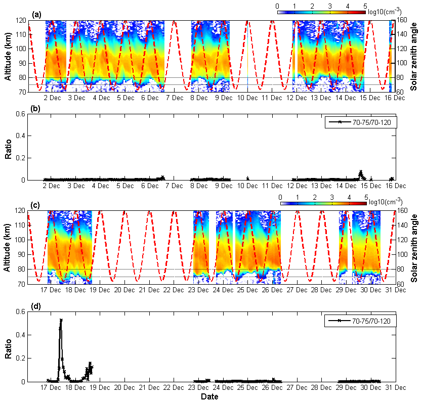
Figure 1 (a, b) The time–height evolution of Na density and the corresponding temporal variation of the ratio of Na density averaged in the altitude range of 70–75 km to that within 70–120 km on 3–9 December 2014. (c, d) The same but on 12–18 December 2014. The solar zenith angle is plotted with red dotted curves in (a) and (c). The two black dashed lines in (a) and (c) denote 80 and 75 km, respectively.

Noteworthy is the much more significant bottom enhancements below 75 km observed in mid-December (i.e., on 14, 17, and 18 December; there are data gaps during 15–16 December), as can be seen in Fig. 1a and c. The pronounced Na bottom enhancements between 70 and 75 km on 14, 17, and 18 December are also shown in Fig. 1b and d by the temporal variation of the ratio of Na density averaged within 70–75 km to that within 70–120 km. The most intriguing result appears in the early morning of 17 December when Na atom density around 75 km even reaches up to the same order of magnitude as the peak density of the Na main layer.

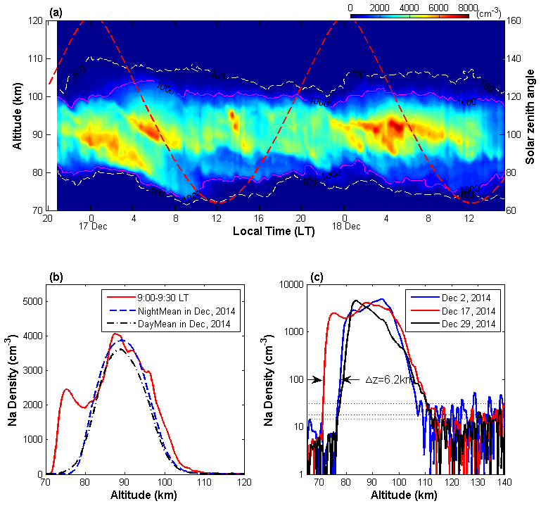
Figure 2 (a) Contours of Na density versus local time and altitude observed from ∼ 21:00 LT on 16 December to ∼ 16:00 LT on 18 December 2014. The time resolution is 15 min, and altitude resolution is 960 m. (b) Comparison of Na density profiles averaged at 09:00–09:30 LT on 17 December (red solid line), and averaged during daytime (07:00–17:00 LT, black dotted line) and nighttime (17:00–07:00 LT, blue dashed line) in December 2014. (c) Comparison of Na density profiles on 17 December (red curve) with those on 2 December (blue curve) and 29 December (black curve). The horizontal dotted lines are their respective detection limits, whose values from small to large are ∼ 15, 19, 31 cm⁻³.

Figure 2a shows the Na density contour in time–altitude over about 43 h from ∼ 21:00 LT on 16 December to ∼ 16:00 LT on 18 December 2014 in a linear scale. The variation of the solar zenith angle is also plotted with a red dashed line. It can be seen that the constant density line of 100 cm⁻³ (white dashed line) on the Na layer bottom moves downward from ∼ 80 km before 04:00 LT to ∼ 71.5 km around 09:15 LT on 17 December then it oscillates at this lower altitude until ∼ 17:00 LT when it begins to recover upward to above 75 km. The constant density line of 1000 cm⁻³ (pink solid line) on the layer bottom shows a similar downward movement in the early morning of 17 December and reached its lowest altitude at ∼ 72 km around 09:15 LT, however it rapidly recovered upward by over 5 km at around 11:00 LT. Figure 2b displays the vertical profile of Na number density averaged at 09:00–09:30 LT on 17 December (red solid line), along with the averaged nocturnal and daytime Na profiles in December 2014 (blue dashed and black dotted lines, respectively). It clearly shows the pronounced Na density enhancement below 80 km on 17 December. The Na density around 75 km reaches to ∼ 2500 cm⁻³, which is nearly 2 orders of magnitude larger than the daytime mean value of this month at a similar altitude. This implies interesting and complicated atmospheric physical and chemical processes. In order to further clarify the very significant bottom enhancement on 17 December in Fig. 2c, we also compared the Na density profile on 17 December (red curve) with those on 2 December (blue curve) and 29 December (black curve), which can represent the cases in early and late December, respectively. The Na density profiles in Fig. 2c are also the results averaged at 09:00–09:30 LT for each day and plotted in logarithmic coordinates. The dotted lines are their respective detection limits that are given by 1.5 times of the standard deviation of the background noise (Gao et al., 2015). The detection limit for the density profile on 17 December is ∼ 15 cm⁻³. The altitude difference between 17 December and the other 2 d is as large as ∼ 6.2 km for the density of 100 cm⁻³.

In the early morning of December 18, Na density increase on the layer underside below 75 km can also be seen, but it is evident from Fig. 2a that the bottom enhancement is less intense as compared to the previous day (17 December). It is noted that the Na main layer is also very different between the two adjacent days. The Na layer observations between 22:00 LT on 16 December and 12:00 LT on 17 December shows an apparent double-peak structure with downward phase propagation. The first peak which appears around 22:00 LT near 92 km descends at a rate of ∼ 0.5 m s⁻¹. The second peak appears around 04:00 LT and 95 km, and also shows a similar downward propagation phase speed. The strong bottom extension in the morning of 17 December follows well the downward propagation trend of the first peak in the main layer, but its peak density rapidly decreases below 80 km.

4 Discussion

The Na layer observational results presented in Sect. 3 reveal more significant bottom extensions as low as ∼ 72 km in mid-December 2014 (i.e., 14, 17, and 18 December, as shown in Fig. 1) compared to the normal results observed on other days in December. Another noteworthy feature is the striking bottom enhancement with an unprecedented density of ∼ 2500 cm⁻³ around 75 km in the morning of 17 December.

Theories and model simulations of the metal layer (Cox et al., 2001; Plane, 2004; Plane et al., 2015) indicated that the chemical lifetime of Na atoms near the Na layer peak is much longer than the timescale of vertical transport, thus the dynamical processes dominate the Na density variation between 85 and 95 km (Xu and Smith, 2003), while near the bottom of Na layer, Na chemistry plays a more significant role (Self and Plane, 2002). According to Plane et al. (2015), here we simply describe the main Na chemical reactions that determine the Na variations on the bottom side of the layer:

$$\begin{array}{}\text{(R1)}& {\displaystyle }\mathrm{Na}+{\mathrm{O}}_{\mathrm{3}}\to \mathrm{NaO}+{\mathrm{O}}_{\mathrm{2}}\mathrm{1.1}\times {\mathrm{10}}^{-\mathrm{9}}\exp (-\mathrm{116}/T)\text{(R2)}& {\displaystyle }{\mathrm{NaHCO}}_{\mathrm{3}}+h\mathit{\nu }\to \mathrm{Na}+{\mathrm{HCO}}_{\mathrm{3}}\mathrm{1.3}\times {\mathrm{10}}^{-\mathrm{4}}\text{(R3)}& {\displaystyle }\begin{array}{rl}& {\mathrm{NaHCO}}_{\mathrm{3}}+\mathrm{H}\to \mathrm{Na}+{\mathrm{H}}_{\mathrm{2}}{\mathrm{CO}}_{\mathrm{3}}\\ & \left(\mathrm{1.84}\times {\mathrm{10}}^{-\mathrm{13}}\right)T^{\mathrm{0.777}}\exp (-\mathrm{1014}/T).\end{array}\end{array}$$

Units: unimolecular, s⁻¹; bimolecular, cm³ molecule⁻¹ s⁻¹.

The neutral Na chemistry on the underside of the Na layer is mainly controlled by odd oxygen (O and O₃) and hydrogen (H) chemistry. Through oxidation reaction of Na with O₃, Na is converted to NaO (or further oxidized to NaO₂, NaO₃) (Reaction R1), which can further react with H₂O or H₂ and CO₂ (and O₂) to form the relatively stable NaHCO₃, which is believed to be the major reservoir species for Na (Plane et al., 2015; Gomez Martin et al., 2016). The oxidation reaction of Na atoms (Reaction R1) is greatly accelerated with altitude decrease as it is sensitive to pressure (Yuan et al., 2019). NaO and NaO₂ produced by the oxidation are short-lived according to Self and Plane (2002). They can also be recycled back to Na by atomic O. As atomic O has a large positive vertical gradient near the mesopause region, the chemical lifetime of Na atoms is extremely short (only several seconds) on the underside of the Na layer around and below 80 km (Xu and Smith, 2005), and most of Na is in the form of NaHCO₃. This also results in a sharp lower edge of Na layer near 80 km.

During daytime, solar radiation will significantly accelerate the photolysis reaction of NaHCO₃, thus a part of NaHCO₃ can be converted back to Na atoms (Reaction R2). NaHCO₃ can also be recycled back to Na by reaction with H (Reaction R3). The reaction rate of NaHCO₃ with H positively depends on background temperature. The photolysis of O_2, O₃ and H₂O during the day can greatly increase the concentrations of atomic O and H around and below 80 km (Plane, 2003), thus further promoting the release of Na atoms from NaHCO₃ or NaO and NaO₂. Generally, the typical daytime H concentration is ∼ 2–5 × 10⁷ cm⁻³ between 75 and 80 km (Plane et al., 2015; Yuan et al., 2019), and mesopause temperature is ∼ 200 K, resulting in that the first-order rate of Reaction (R3) is dozens of times slower than that of Reaction (R2). Thus, photolysis reaction of NaHCO₃ is often considered to dominate the increase in Na concentration on the layer bottom after sunrise (Yuan et al., 2019). Photolysis of other Na species can also contribute to Na density increase. However, the bottom extensions downward to ∼ 72 km are not seen in early and late December even though the variation of solar illumination with local time is similar in the same month. Moreover, the variations of Na layer bottom on 17 December are inconsistent with that of solar zenith angle. For example, the constant density line of 1000 cm⁻³ on the layer bottom rapidly recovers upward before midday when there is still solar illumination. This implies that the photolysis reactions driven by solar radiation is not the most critical factor responsible for the significant bottom extensions and enhancements of Na layer below 75 km observed in mid-December 2014.

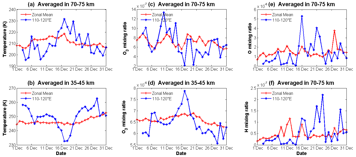
Figure 3 (a, b) Temperature variations in December 2014 from the SABER instrument onboard TIMED satellite, averaged in the altitude range of 70–75 and 35–45 km, respectively. (c, d) The same as (a)–(b) but for mixing ratio of O₃. (e, f) The variations of mixing ratio of atomic H and O in December 2014 from SABER, averaged in the altitude range of 70–75 km. The red lines with pluses in each plot represent the daily and zonal mean results averaged between 35 and 45^∘ N, and the blue lines with asterisks represent the daily mean results averaged near the lidar site (35–45^∘ N, 110–120^∘ E).

According to the Na neutral chemical reactions (Reactions R1, R3), Na density evolution on the layer bottom are strongly dependent on temperature and the concentrations of background minor chemical constituents (e.g., O₃, H and O). Thus we analyze their variations in December 2014, which are shown in Fig. 3a–f, respectively. Figure 3a–b plots the daily mean temperature variation averaged in the altitude range of 70–75 and 35–45 km, respectively, in December 2014 from the SABER instrument. The red dotted lines represent the zonal mean (35–45^∘ N) results, and the blue solid lines represent the results averaged over latitudes of 35–45^∘ N and longitudes of 110–120^∘ E, i.e., taking the averaged measurement profiles of the lidar site overpasses within a range of ∼ ±5^∘ in latitude and ∼ ±5^∘ in longitude. As can be seen, there are apparent temperature anomalies with opposite phase between upper stratosphere and upper mesosphere in mid-December over the lidar site (blue solid lines with asterisks), when compared to the zonal mean temperature (red solid lines with pluses). The temperature in the altitude region of 70–75 km over the lidar site is increased by nearly 30 K within 1 week. During the same period (15–20 December), the local stratosphere shows ∼ 15–20 K cooler than the zonal mean temperatures between 35 and 45 km.

The variations of Na chemistry-related background atmospheric species (e.g., O₃, H and O) can also be obtained from TIMED–SABER instrument (Fig. 3c–f). Compared to the temporal variation of zonal mean value, the averaged O₃ mixing ratio near the lidar site (35–45^∘ N, 110–120^∘ E) shows weak negative perturbation between 70 and 75 km, while showing positive perturbation between 35 and 45 km in mid-December. Clear positive perturbations of the mixing ratios of atomic H and O averaged between 70 and 75 km over the lidar site are also observed in mid-December. For example, the mixing ratio of atomic H is increased by over 5 times on 17 December (from less than 0.2 × 10⁻⁷ to over 1 × 10⁻⁷), as shown in Fig. 3f. It is intriguing that the duration of background atmospheric anomalies over the lidar site (Fig. 3a–f) coincides well with that of the significant Na density enhancement below 75 km shown in Fig. 1. This implies that the neutral chemistry reaction (Reaction R3) makes a critical contribution to the observed Na enhancements on the layer bottom in mid-December. With a temperature of T = 230 K (corresponding to a rate of R₃≈1.6 × 10⁻¹³ cm³ molecule⁻¹ s⁻¹) and H density of 1 × 10⁸ cm⁻³ (estimated according to the mixing ratio of atomic H and atmospheric density in the region between 70 and 75 km), the production rate of Na via reaction of NaHCO₃ with H is estimated to be increased by nearly 10 times compared with that under the typical mesopause atmospheric condition in winter of middle latitude in the Northern Hemisphere (T = 200 K, R₃≈7.2 × 10⁻¹⁴ cm³ molecule⁻¹ s⁻¹, and assuming atomic H concentration to be 2 × 10⁷ cm⁻³ between 70 and 75 km). Furthermore, considering the contribution by increase in atomic O and decrease in O₃ concentration near the mesopause region, which facilitate the liberation of Na atoms and restrict the removal of Na atoms via oxidation reaction respectively (Plane et al., 2015), the net production rate of atomic Na through neutral chemical reactions is expected to be faster than the estimation. Therefore, the neutral chemical reactions, accelerated by warming of upper mesosphere and increase of atomic H and O concentrations, play a critical role in the significant bottom extensions and enhancements of the Na layer below 75 km in mid-December. Undoubtedly, the photolysis of NaHCO₃ also contributes to the intense bottom extension of the Na layer after sunrise.

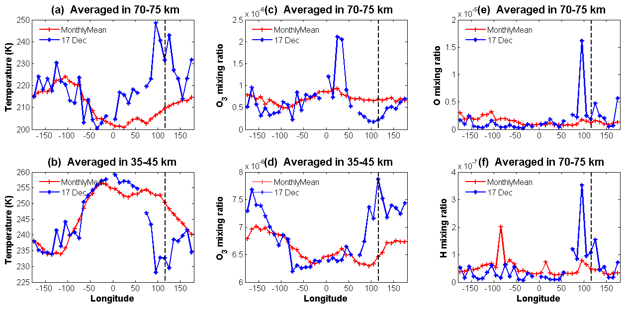
Figure 4 (a, b) Temperature variation with longitude, averaged between 35–45^∘ N in the altitude range of 70–75 and 35–45 km, respectively. (c, d) The same as (a)–(b) but for mixing ratio of O₃. (e, f) The variations of mixing ratio of atomic H and O with longitude, averaged between 35–45^∘ N in the altitude range of 70–75 km. The red lines with pluses represent the monthly mean results in December 2014, and the blue lines with asterisks represent the daily mean results on 17 December. The black dotted lines in each plot indicate the longitude of the lidar site. Each data point is obtained by averaging within a longitude range of 10^∘.

These anomalous structures in background atmosphere over the lidar site appearing in mid-December 2014 can be further verified in Fig. 4. Figure 4a–b shows the longitudinal variations of temperature averaged between 35–45^∘ N in the altitude range of 70–75 and 35–45 km, respectively. The red lines with pluses and blue lines with asterisks represent the monthly and daily (taking 17 December for example) mean results, respectively. The monthly mean temperatures in both the upper mesosphere and stratosphere regions show a wavy structure of zonal wavenumber 1. In Fig. 4a–b, apparent anomalous temperature structures with opposite phase between the upper mesosphere and the stratosphere are seen on 17 December compared to the monthly mean results, and this extends across a longitude range of nearly 100^∘, covering the lidar site (116.01^∘ E). The longitudinal variations of minor chemical constituents averaged between 35–45^∘ N are plotted in Fig. 4c–f, respectively. Similarly, negative perturbations of O₃, and positive perturbations of atomic H and O averaged in the altitude range of 70–75 km near the lidar site can be clearly seen in the daily mean results on 17 December.

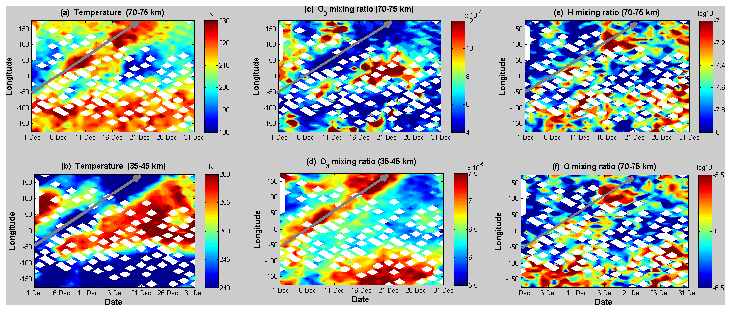
Figure 5 (a–d) The temporal variations of temperature and O₃ with longitude averaged over 35–45^∘ N and in the altitude range of 70–75 and 35–45 km, respectively. (e–f) The daily variations of atomic H and O with longitude, averaged over 35–45^∘ N and in the altitude range of 70–75 km, respectively.

The synchronous and out-of-phase atmosphere anomalies between the upper stratosphere and mesosphere over the lidar site in mid-December, together with the fact that these anomalies lasted for several days, imply that they are most likely linked to PW activities. Figure 5 shows the temporal–longitudinal variations in temperature and neutral chemical species averaged in 35–45^∘ N in the upper stratosphere (35–45 km) and the upper mesosphere (70–75 km) in December 2014 observed by SABER/TIMED. Figure 5a–f shows clear eastward planetary-scale perturbations in these background atmospheric parameters, and the atmospheric anomalies appearing in mid-December near the Na lidar site are shown to be the result of the zonal shifting perturbation structure transporting from west to east.

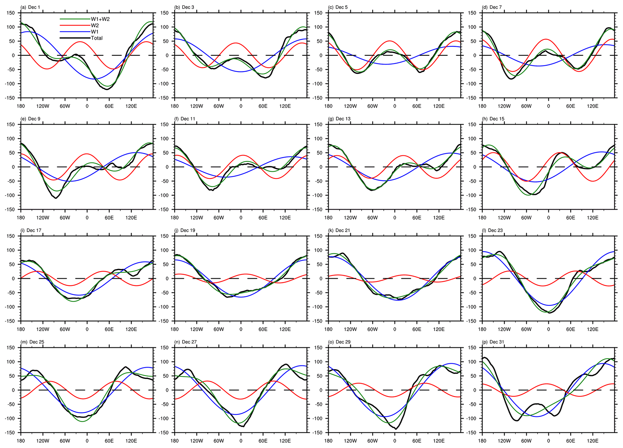
Figure 6 Longitudinal distributions of geopotential amplitudes of PWs for 1–31 December 2014 (shown on every other day; black: total; blue: PW1; red: PW2; and green: PW1+PW2).

It is worth mentioning that the cooling anomaly in the stratosphere and warming anomaly in the mesosphere are exactly the opposite of the temperature anomalies observed during the well-known sudden stratosphere warming (SSW) event appearing in high latitudes. Yuan et al. (2012a) reported that a significant decrease in Na abundance below 90 km was observed at 41^∘ N during the 2009 SSW event, which is consistent with the dramatic cooling in this region. Feng et al. (2017) also investigated the responses of metal layers to the 2009 major SSW, and substantial depletions of the Na and Fe layers were seen both from the lidar measurements and model simulations mainly due to the mesospheric cooling. Sudden enhancement of PWs and their interactions with the mean flow are widely accepted as the cause of SSWs (Matsuno, 1971). We further use ERA-Interim reanalysis to calculate the longitudinal distributions of geopotential amplitudes of PWs in the stratosphere. Figure 6 shows the zonal distribution of geopotential height amplitudes (unit: gpm) at 10 hPa (∼ 32 km) and 45^∘ N in December 2014. It can be seen that before mid-December, planetary wave number 2 (PW2) is unusually strong and the amplitude of PW2 is even larger than that of PW1. The PW2 trough (low geopotential height associated with cold air) moves eastward to the longitude of the lidar site (∼ 116^∘ E) near 15 December, resulting that this region was dominated by cold air mass. After 17 December, the amplitude of PW2 significantly decreases and PW1 increases. PW1 ridge (high geopotential height associated with warm air) starts to dominate the region near the lidar site. This demonstrated that the atmospheric temperature anomalies in the stratosphere in mid-December 2014 around the lidar region was indeed related to the unusual PW activity. According to Smith (1996), the planetary-scale disturbances might be generated in situ by longitudinal variations of gravity wave (GW) forcing in the mesosphere due to the GW filtering by PWs in the stratosphere. The opposite phase of anomalies between the stratosphere and mesosphere are likely caused by the interaction with gravity waves (GWs) (Limpasuvan et al., 2012). It is noted that indeed a minor SSW occurred about half a month later (in early January 2015). However, a detailed investigation on this aspect is beyond the scope of the present work.

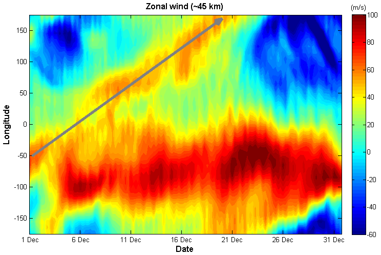
Figure 7 The temporal variation of zonal wind with longitude, averaged over 35–45^∘ N near 45 km obtained from ERA-Interim global atmospheric reanalysis data.

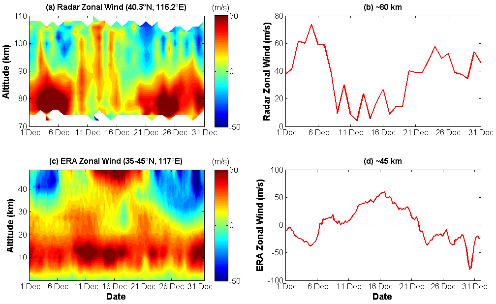
Figure 8 (a, c) The temporal variations of zonal wind with altitude near the lidar site in December 2014 obtained from meteor radar (70–110 km, 40.3^∘ N, 116.2^∘ E) and ERA reanalysis data (0–48 km, 35–45^∘ N, 117^∘ E), respectively; (b, d) the temporal variations of zonal wind near 80 and 45 km, respectively (red lines). The blue dashed lines indicate zero wind.

The stratosphere zonal wind, averaged over 35–45^∘ N near 45 km obtained from ERA-Interim global atmospheric reanalysis also exhibit eastward transporting structure of westerly wind, which is consistent with the temporal–longitudinal variation of temperature and minor constituents in December 2014 (as indicated by the gray arrow in Figs. 5 and 7). As shown in Fig. 8a–b, the zonal wind results observed by a meteor radar located near the lidar site reveal apparent westerly wind deceleration of over 50 m s⁻¹ in the upper mesosphere region near 80 km, and simultaneous easterly wind reversal above 90 km in mid-December. During almost the same time period, the zonal wind in the upper stratosphere changes direction from easterly to westerly (Fig. 8c–d). In late December, the zonal wind in the upper mesosphere and the upper stratosphere recovers to the large westerly wind and easterly wind, respectively. The zonal wind reversal from westward to eastward in the upper stratosphere and deceleration of eastward zonal wind in the upper mesosphere in mid-December are close in time to the appearance of the anomalies of temperature and minor chemical constituents over the lidar site.

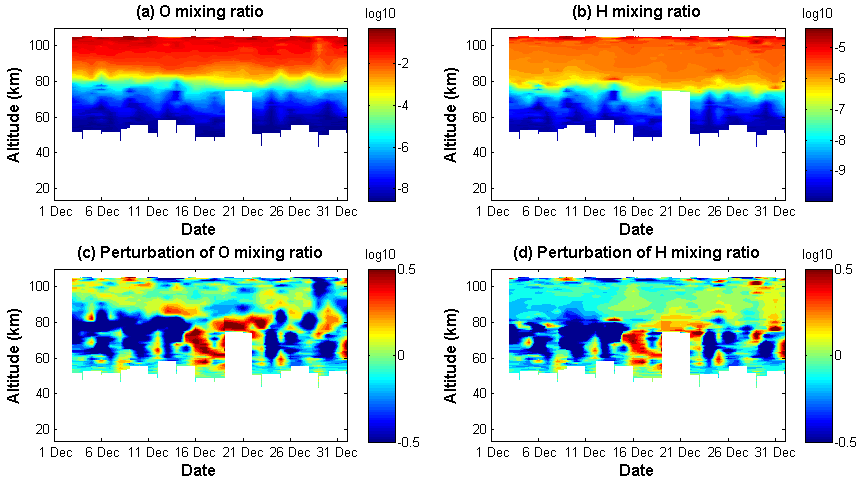
Figure 9 (a, b) The temporal and altitude variations of mixing ratio (in logarithm coordinates) of atomic O and H obtained from SABER/TIMED. The data within 35–45^∘ N and 110–120^∘ E were averaged. (c, d) Their perturbations obtained by subtracting the monthly mean vertical profiles.

Previous works have demonstrated the importance of the stratosphere wind filtering in controlling the propagation of atmospheric waves to the upper mesosphere region (e.g., Siskind et al., 2010). The out-of-phase temperature anomalies in the upper stratosphere and upper mesosphere in mid-December hint at their coupling likely through interaction of PW with mean flow and changing the GW filtering by the stratospheric wind. The westerly zonal wind in the stratosphere (as shown in Figs. 7 and 8c) can induce filtering of eastward-propagating GWs and penetration of westward-propagating GWs into the mesosphere (Chandran et al., 2011). The westward-propagating GWs induce a downward circulation in the mesosphere causing adiabatic heating (Liu and Roble, 2002, 2005; Yamashita et al., 2010). Therefore, the dramatic cooling and heating in the stratosphere and the mesosphere in mid-December are likely caused by the perturbations of PWs and their interaction with GWs (Marsh, 2011; Marsh et al., 2013; Limpasuvan et al., 2012 and references therein). The strong perturbations of O₃ with zonal shift in the stratosphere and upper mesosphere (Fig. 5c–d) are likely to be linked to the consistent temperature perturbations (Fig. 5a–b). The reaction rate of O₃ production ($\mathrm{O}+{\mathrm{O}}_{\mathrm{2}}+\mathrm{M}\to {\mathrm{O}}_{\mathrm{3}}+\mathrm{M}$) increases with decreasing temperature (Smith and Marsh, 2005), thus the decrease of temperature in the stratosphere shifts the O $/$ O₃ ratio towards O₃, resulting in the increase of O₃. And then the upper mesosphere becomes the opposite situation to that in the stratosphere. The temporal variation of atomic H and O with longitude (Fig. 5e–f) did not show as obvious zonal shifting structures as seen in O₃. The strong positive perturbations of atomic H and O in the upper mesosphere over the lidar site in mid-December might be also partly associated to the downwelling in the upper mesosphere, which could force H- and O-rich air downward and increase the concentrations of H and O below 80 km as their mixing ratios increase with altitude near 80 km (Marsh et al., 2013; Narayanan et al., 2021). Near 80 km, the vertical gradients of both atomic O and H are very large (as shown in Fig. 9a–b). The positive perturbations in H and O below 80 km in mid-December are also clearly seen in Fig. 9c–d, which was obtained by subtracting the monthly mean vertical profiles from the temporal and altitude variations of mixing ratios of H and O.

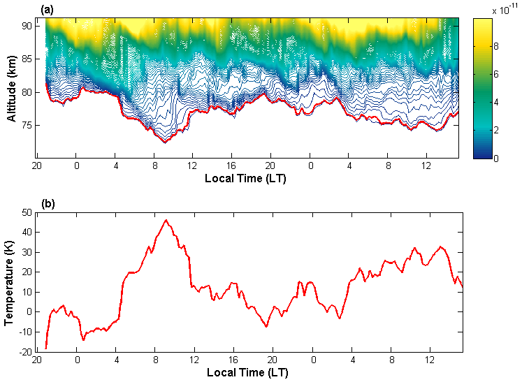
Figure 10 (a) Na mixing ratio corresponding to Fig. 2a; (b) adiabatic vertical motion-induced temperature perturbations calculated from the highlighted Na mixing ratio isopleth (1 × 10⁻¹²) in (a).

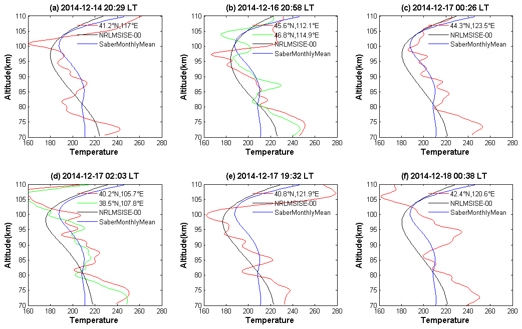
Figure 11 SABER temperature profiles obtained near the lidar location. Blue and black lines in each subplot represent the temperature profiles from the empirical atmospheric model NRLMSISE-00 (Naval Research Laboratory Mass Spectrometer and Incoherent Scatter Radar Exosphere 2000) and monthly average SABER results near the lidar location, respectively.

Comparing the behavior of Na layer on 17 December to that on 14 and 18 December, the most striking feature for the former is the more apparent wavy structures with downward propagation phase. It is worth mentioning that the aircraft Na lidar during the Deep Propagating Gravity Wave Experiment (DEEPWAVE) measurement program observed multiple Na layers descending to 70–72 km over New Zealand in 2014 due to mountain waves (MWs) (Bossert et al., 2015, 2018; Fritts et al., 2016, 2018). The downwelling regions in Fig. 2a seem to repeat on multiple days and are likely due to the superposition of tide and GW. The waves can induce adiabatic vertical motion of the air parcel, leading to adiabatic heating and thereby contributing to the much stronger Na layer bottom enhancement on 17 December. In the absence of chemistry, the GW/tide-induced temperature perturbation due to adiabatic expansion and compression of the air parcel can be approximately calculated according to the vertical displacements of Na mixing ratio isopleths based on the approach in Bossert et al. (2015, 2018). Figure 10a shows the Na mixing ratio contours corresponding to Fig. 2a. The isopleth highlighted in red corresponds to 1 × 10⁻¹² and an average altitude of 77.01 km. In Bossert et al. (2018), the average altitude of each isopleth was used as the undisturbed equilibrium altitude for the temperature perturbation calculation. However, it is unreasonable to use the average altitude (∼ 77.01 km) of the highlighted isopleth here because the observation is diurnal (nearly 44 h), and the Na mixing ratio is largely affected by photochemistry. If we choose the isopleth between 22:00 and 24:00 LT (before the descending layer formation) on 17 December, the average altitude is calculated to be 78.74 km, and the corresponding temperature perturbation for the highlighted isopleth in Fig. 10a is shown in Fig. 10b. Taking into account the chemistry which depends strongly on temperature, Bossert et al. (2018) employed a model of Na chemistry to determine the chemical amplification factor (CAF) of atomic Na. The CAF was then used to correct the calculated temperature perturbations from Na mixing ratio. For a mean height of 81.5 km and a wave with period of 20 min turned on 1 h after sunset, the largest CAF of atomic Na is ∼ 1.6 within 4 h after sunset. However, the effect of chemistry on the underside of the Na layer would be greater during daytime. After sunrise, solar radiation will significantly accelerate the photolysis reaction of NaHCO₃, and convert NaHCO₃ back to Na atoms (Reaction R2). In addition, the photolysis of O₂, O₃, and H₂O during the day can greatly increase the concentrations of atomic O and H around and below 80 km (Plane, 2003), thus further promoting the release of Na atoms from NaHCO₃ (Reaction R3) or NaO and NaO₂. Therefore the CAF will increases significantly and be much larger than 1.6 after sunrise, especially at lower altitudes (i.e., below 80 km). The GW-induced adiabatic temperature perturbations on 17 December would be much smaller than the roughly estimated values shown in Fig. 10b. In order to properly estimate the adiabatic temperature change associated with the downwelling forced by the superposition of GW and tide, a more comprehensive model investigation may be needed.

Actually, before the strong downwelling regions appear, the SABER sampling profile obtained at ∼ 20:58 LT on 16 December around the lidar site already shows considerable positive perturbations (∼ 30 K) at around 75 km, as shown in Fig. 11b. The temperature profiles obtained at ∼ 00:26 and 02:03 LT on 17 December (Fig. 11c–d) also have warming anomalies around 75 km. However, the Na mixing ratio isopleths moved down to below 80 km after ∼ 04:00 LT. The temperature anomalies also appeared on other days near mid-December (e.g., 14, 18 December, as shown in Fig. 11a, f). These imply that the temperature perturbations near 75 km observed by SABER are more likely linked to the GW filtering by PW rather than the strong downwelling caused by the superposition of tide and GW.

Given all of that, we suggest two causes for inducing adiabatic heating and contributing to the observed more significant bottom enhancement on 17 December. One is the interaction of PW with mean flow which could change GW filtering properties by the stratospheric wind (Yamashita et al., 2010; Liu and Roble, 2002). This occurs over a relatively large horizontal area as seen in Figs. 4 and 5 (covering nearly 50^∘ in longitude around the lidar site and lasting several days in mid-December, i.e., on 14, 18 December, in addition to 17 December). The other is the superposition of tide and GW, which induces the stronger downwelling on 17 December as shown in Fig. 2. The effect of the latter is more significant than the former as we see the bottom enhancement on 17 December is much more pronounced than that observed on 14 and 18 December.

5 Conclusions

In this study, we report the observations of significant extension of Na layer bottom by a diurnal Na lidar in mid-December 2014 at Beijing (40.41^∘ N, 116.01^∘ E), China. Considerable Na atoms are observed even as low as ∼ 72 km. Liberation of Na atoms from its reservoir (e.g., NaHCO₃) near the Na layer bottom via neutral chemical reactions, which are accelerated by the largely increased temperature and concentrations of atomic H and O, is suggested to be the critical production mechanism of the enhanced Na layer below 75 km. The diurnal lidar measurements of the Na layer, zonal wind results from a nearby meteor radar, global satellite observations, and reanalysis data presented here reveal the close correlation between the variation of Na layer bottom and planetary-scale atmospheric processes. The longitudinal distributions of geopotential amplitudes of PW show that there exists unusual development of the amplitude of PW2, and the stratosphere near the lidar location is dominated by PW2 trough in mid-December. The out-of-phase temperature anomalies in the upper stratosphere and upper mesosphere are likely due to the modulation of GW filtering by stratosphere wind. The strong eastward wind in the upper stratosphere provides a favorable condition for the vertical propagation of westward GWs. Westward forcing could induce a poleward flow and drive downward circulation in the mesosphere, leading to adiabatic heating. The unprecedented Na density of ∼ 2500 cm⁻³ near 75 km observed on 17 December 2014 is also greatly contributed by the adiabatic vertical motion of air parcel forced by the superposition of tide and GW.

The results of this paper provide direct observational evidence for the role of PWs in the perturbations of metal layers in the upper mesosphere region. These results also have implications for the response of the metal layers (especially the layer bottom) to perturbations in the lower atmosphere (i.e., stratosphere). Modeling studies are desirable to investigate the complicated interactions of dynamical and chemical processes and their effects on the variations of metal layer in more depth.