A new method for inferring city emissions and lifetimes of nitrogen oxides from high-resolution nitrogen dioxide observations: a model study

We present a new method to infer emissions and lifetimes of nitrogen oxides (NO_x) based on tropospheric nitrogen dioxide (NO₂) observations together with reanalysis wind fields for cities located in polluted backgrounds. Since the accuracy of the method is difficult to assess due to lack of “true values” that can be used as a benchmark, we apply the method to synthetic NO₂ observations derived from the NASA-Unified Weather Research and Forecasting (NU-WRF) model at a high horizontal spatial resolution of 4 km × 4 km for cities over the continental United States. We compare the inferred emissions and lifetimes with the values given by the NU-WRF model to evaluate the method. The method is applicable to 26 US cities. The derived results are generally in good agreement with the values given by the model, with the relative differences of 2 % ± 17 % (mean ± standard deviation) and 15 % ± 25 % for lifetimes and emissions, respectively. Our investigation suggests that the use of wind data prior to the satellite overpass time improves the performance of the method. The correlation coefficients between inferred and NU-WRF lifetimes increase from 0.56 to 0.79 and for emissions increase from 0.88 to 0.96 when comparing results based on wind fields sampled simultaneously with satellite observations and averaged over 9 h data prior to satellite observations, respectively. We estimate that uncertainties in NO_x lifetime and emissions arising from the method are approximately 15 % and 20 %, respectively, for typical (US) cities. The total uncertainties reach up to 43 % (lifetimes) and 45 % (emissions) by considering the additional uncertainties associated with satellite NO₂ observations and wind data. We expect this new method to be applicable to NO₂ observations from the TROPOspheric Monitoring Instrument (TROPOMI) and geostationary satellites, such as Geostationary Environment Monitoring Spectrometer (GEMS) or the Tropospheric Emissions: Monitoring Pollution (TEMPO) instrument, to estimate urban NO_x emissions and lifetimes globally.

1 Introduction

Nitrogen oxides (NO_x), consisting of nitrogen dioxide (NO₂) and nitric oxide (NO), are important atmospheric trace gases that actively participate in the formation of tropospheric ozone and secondary aerosols and accordingly have a significant effect on human health and climate (Seinfeld and Pandis, 2006). NO_x emission sources include anthropogenic activities, biomass burning, soil emissions, and lightning. Fossil-fuel burning from mobile and industrial emitters represents the largest source of anthropogenic NO_x emissions; these sources are usually clustered near densely populated urban areas (Crippa et al., 2018).

We traditionally rely on a bottom-up method to estimate anthropogenic NO_x emissions for a country or a region based on their total fuel use and averaged emission factors, which are subject to uncertainties due to incomplete understanding of real-world operating conditions and spatial distributions (Butler et al., 2008). Some sources may be missing from bottom-up emission inventories (McLinden et al., 2016). Additionally, estimates of NO_x emissions may become outdated when fuel consumption and emission factors change dramatically. For instance, NO_x emissions from China decreased by 21 % from 2011 to 2015 due to wide deployment of denitration devices (Liu et al., 2016a). Inferring emissions for individual cities is even more challenging, due to the difficulties in acquiring a complete and reliable database for fuel consumptions and emission factors at city level. Proxies such as population density, industrial productivity, and road network maps are often used to downscale national/regional emissions to finer scales, which may incorrectly allocate emission sources spatially (Butler et al., 2008).

Satellite observations of tropospheric NO₂ have been widely used to infer the strength of NO_x emissions. Satellite instruments, e.g., the Ozone Monitoring Instrument (OMI; Levelt et al., 2006, 2018) and TROPOspheric Monitoring Instrument (TROPOMI; Veefkind et al., 2012), are used to retrieve the column density of NO₂ in a vertical column of air. These data can then be related to NO_x emissions by considering chemical conversion and transport. Chemical transport models (CTMs) were initially employed to use NO₂ measured from space as a constraint to improve NO_x emission inventories based on mass balance (e.g., Martin et al., 2003; Kim et al., 2009; Lamsal et al., 2011). Techniques such as the four-dimensional variational (4D-Var) method (e.g., Henze et al., 2007, 2009), extended Kalman filter (e.g., Ding et al., 2017), ensemble Kalman filter (e.g., Miyazaki et al., 2017), and hybrid mass balance/4D-Var (e.g., Qu et al., 2019) have also been used to improve emissions estimates within CTMs.

Several studies have inferred emissions independent of CTMs (e.g., Beirle et al., 2011; Liu et al., 2017; Laughner and Cohen, 2019). Such investigations were inspired by a pioneering study that used the downwind decay of NO₂ in continental outflow regions to estimate the global NO_x lifetime and total emissions (Leue et al., 2001). Beirle et al. (2011) first proposed an empirical function to describe the plume distribution around an isolated city without inputs from CTMs. Follow-up studies have adopted this function to provide estimates of NO_x emissions from power plants and cities based on OMI (e.g., de Foy et al., 2015 and Lu et al., 2015) and TROPOMI (e.g., Goldberg et al., 2019) observations. Additional methods, such as the plume rotation technique (Pommier et al., 2013; Valin et al., 2013) and the divergence approach (Beirle et al., 2019), were developed to refine the approach of Beirle et al. (2011). More recent studies explored additional constraints for the empirical function using simulated atmospheric composition from models (e.g., Lorente et al., 2019; Lange et al., 2021). For sources with a polluted background, Liu et al. (2016b) proposed a different fitting function to consider the interferences from surrounding sources; this approach has been used to estimate NO_x emissions for European cities (Verstraeten et al., 2018).

The uncertainties in satellite-derived emissions inferred from CTM-independent approaches have rarely been investigated. Field campaigns, e.g., Deriving Information on Surface Conditions from Column and Vertically Resolved Observations Relevant to Air Quality (DISCOVER-AQ), Korea–United States Air Quality Study (KORUS-AQ), and Cabauw Intercomparison of Nitrogen Dioxide Measuring Instruments 2 (CINDI-2), have been performed to better quantify errors in the NO₂ observations (e.g., Choi et al., 2020) and therefore improve knowledge about uncertainties in satellite-derived emissions. Existing studies usually quantify the uncertainties based on results from sensitivity analyses (e.g., Beirle et al., 2011), since we usually lack “true values” that can be used as a benchmark for validation. De Foy et al. (2014) tested CTM-independent approaches using simulated NO₂ column densities from a single-point source with a specified emission and chemical lifetime. The good consistency between the derived values and the specified values given to drive the simulation suggests that the uncertainty of the Beirle et al. (2011) approach is small for an ideal, isolated source. However, the performance of the approach in the real world with complex source distributions has not yet been evaluated.

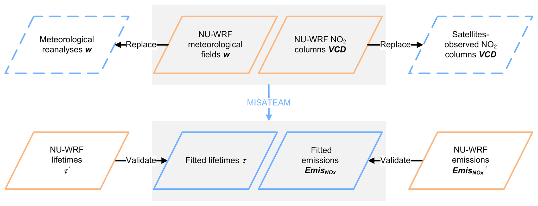
Figure 1 Schematic of our evaluation system to assess the accuracy of the inferring NO_x lifetimes and emissions derived from MISATEAM. The blue symbols represent the inputs (dashed line) and outputs (solid line) of MISATEAM. The orange symbols represent the information derived from NU-WRF.

Here, on the basis of previous approaches (Beirle et al., 2011; Liu et al., 2016b), we develop a new CTM-independent approach for inferring NO_x lifetimes and emissions for cities with polluted backgrounds and complex spatial distribution of interfering emissions. We use synthetic NO₂ observations derived from a model simulation to evaluate the performance of the new approach and to estimate its uncertainties. An overview of the synthetic observations, the methodology and features of the new CTM-independent approach is provided in Sect. 2. We evaluate results by comparing the inferred emissions and lifetimes with values from the model simulation in Sect. 3.1. Section 3.2 compares the performance of the method developed in this work with previous approaches (Beirle et al., 2011; Liu et al., 2016b). Section 3.3 discusses the uncertainties of NO_x lifetimes and emissions derived from the new approach. Section 4 presents a summary of the performance of the new method and future work plans for applying the method to satellite observations.

2 Data and method

In this section, we develop an evaluation system to assess the performance of our newly developed CTM-Independent SATellite-derived Emission estimation Algorithm for Mixed-sources (MISATEAM). Figure 1 displays the schematic of the evaluation system. MISATEAM uses satellite retrievals of tropospheric NO₂ vertical column densities (VCDs), together with wind information from a meteorological reanalysis, to infer NO_x lifetimes and emissions for cities. Cities are usually non-isolated sources with polluted backgrounds (Fig. S1 in the Supplement). Additionally, emissions from cities may spread out and make cities not (quasi) point sources, even at the footprint of satellite observations (a few kilometers; Fig. 3). We refer to these cities as mixed sources.

To evaluate MISATEAM, we replace satellite observations with synthetic NO₂ VCDs derived from the NASA-Unified Weather Research and Forecasting (NU-WRF) model (Tao et al., 2013; Peters-Lidard et al., 2015) (Sect. 2.1). We then apply MISATEAM to the synthetic NO₂ VCDs and NU-WRF meteorological fields to infer urban NO_x lifetimes and emissions (Sect. 2.2). We investigate the impact of temporal variations in wind fields on derived NO_x lifetimes and emissions (Sect. 2.3). In Sect. 2.4, we describe the benchmark NO_x emissions directly given by NU-WRF and NO_x lifetimes deduced from known NO_x emissions and concentrations (hereafter referred to as “given emissions and NU-WRF lifetimes”) that we will compare with the MISATEAM-derived lifetimes and emissions. Analysis of the uncertainties in these datasets, including satellite observations and wind fields, is outside the scope of the study. We briefly discuss the potential impact of ignoring systematic errors in Sect. 3.3.2.

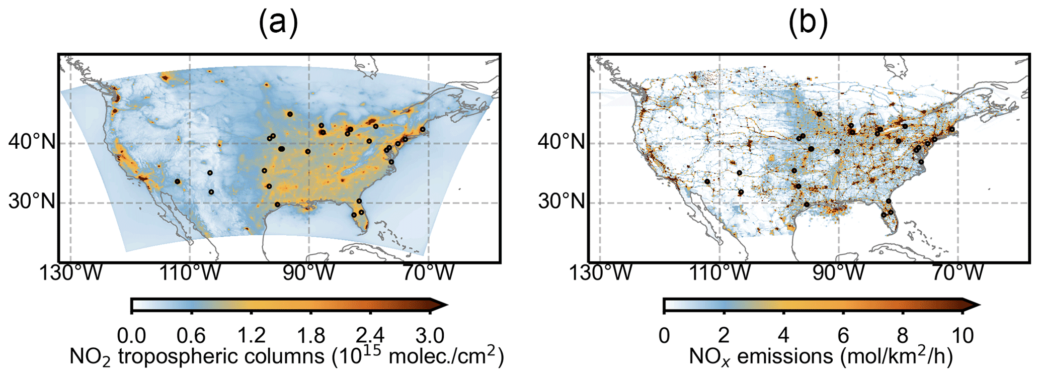
Figure 2 Domain used for simulation. (a) Mean NU-WRF tropospheric NO₂ vertical column densities. (b) Mean NEI NO_x emissions fluxes used to drive the NU-WRF simulation. Hourly mean data at 14:00 LT are averaged from April through September 2016. Locations of the 26 cities investigated in this study are shown by circles (see Sect. 3).

2.1 Synthetic NO₂ VCDs: NU-WRF simulations

We use a regional modeling system, NU-WRF (Tao et al., 2013; Peters-Lidard et al., 2015), to simulate tropospheric NO₂ VCDs over the continental United States. NU-WRF was developed from the advanced research versions of WRF (Michalakes et al., 2001) and WRF-Chem (Grell et al., 2005) with the addition of several NASA-developed components (e.g., Chou and Suarez, 1999; Chin et al., 2002, 2007; Kumar et al., 2006; Peters-Lidard et al., 2007; Shi et al., 2010). The gas-phase chemical mechanism in NU-WRF is the second-generation regional acid deposition model (RADM2; Gross and Stockwell, 2003). The aerosol module is the Goddard Chemistry Aerosol Radiation and Transport (GOCART) model (Chin et al., 2002). We use the anthropogenic emissions based on the 2011 National Emissions Inventory (NEI) compiled by the US Environmental Protection Agency (US EPA, NEI 2011) but with a few modifications, in which the measurements from OMI, the ground-based Air Quality System (AQS), the in situ continuous emissions monitoring in power plants, and the Air Pollutant Emissions Trends Data compiled by the US EPA (https://www.epa.gov/air-emissions-inventories/air-pollutant-emissions-trends-data, last access: 1 December 2021) have been employed to adjust the baseline emissions to the simulation year of 2016 (Tong et al., 2015; Tao et al., 2020). As such, the total anthropogenic NO_x emissions in 2016 were approximately 72 % of those in 2011, the baseline NEI year. The simulation also includes the fire emissions from the Global Fire Data version 4 with small fires (GFED v4s; van der Werf et al., 2017; Randerson et al., 2015); biogenic emissions from the online calculation using the Model of Emissions of Gases and Aerosols from Nature version 2 (MEGAN2; Guenther et al., 2006); dust emissions from the online estimation based on the surface wind speed, soil moisture, and soil erodibility (Ginoux et al., 2001; Kim et al., 2017); and sea salt emissions from the online computation based on the method by Gong (2003).

We run NU-WRF for 2016 at a high horizontal spatial resolution of 4 km × 4 km and 40 vertical layers extending from the surface to 50 hPa in this study. Figure 2 illustrates the domain of the simulation, which covers the continental United States. We integrate NO₂ concentrations from the surface to the tropopause to calculate tropospheric NO₂ VCDs. We assume a consistent tropopause height of 10 km over the model domain to accelerate the data process because NU-WRF outputs do not include tropopause height, and NO₂ VCDs integrated above 10 km increase slightly. We have performed a sensitivity analysis by integrating NO₂ concentrations from the surface to altitudes ranging from 8 to 16 km, where the seasonal mean tropopause heights may occur over the United States (Pan et al., 2011; Rieckh et al., 2014). The derived NO₂ VCDs over the fit domain of individual cities vary slightly above 10 km, with the relative difference of 3 % ± 2 % when increasing the integration altitude from 10 to 12 km, since most NO₂ stays near the surface over the polluted urban areas. The meteorological initial and lateral boundary conditions are derived from the Modern Era Retrospective-Analysis for Research and Applications version 2 (MERRA-2; Rienecker et al., 2011; Gelaro et al., 2017). The chemical initial and lateral boundary conditions are derived from the results of the Community Atmosphere Model with chemistry (CAM-chem; Lamarque et al., 2012). A 7 d model spin-up following the recommendation by Berge et al. (2001) is used.

Figure 2a illustrates the 6-month average of the simulated hourly mean tropospheric NO₂ VCDs sampled at 14:00 LT, which approximately corresponds to the early afternoon overpass time of OMI and TROPOMI. The NO_x emissions used to drive NU-WRF over the model domain for the same time period are presented in Fig. 2b. We focus on cities with populations > 200 000, which have been defined as medium-size urban areas in Organisation for Economic Co-operation and Development (OECD) countries. Nearby cities (located within 50 km of the largest city in a given urban area) are considered as one city cluster when applying MISATEAM to infer lifetimes and emissions. Cities on the boundary of the model domain, e.g., Seattle and San Francisco, are excluded from the following analysis because the data for their inflow/outflow plumes are partially missing from the model output and thus do not meet the requirements of MISATEAM (see details of the fit interval in Sect. 2.2). This filtering results in a total of 60 cities and urban conglomerations (see Table S1 in the Supplement) as the candidates for applying MISATEAM, of which 26 have valid results. The locations of the 26 cities are shown in Fig. 2. Cities without valid results either lack observations under calm wind conditions or are associated with large fitting errors (see details in Sect. 3.1).

2.2 Emission estimation algorithm

We develop MISATEAM based on the methods of Beirle et al. (2011) and Liu et al. (2016b). We develop a new model function aiming for determining emissions for mixed sources, instead of isolated sources, within a clean background considered by Beirle et al. (2011). It is also different from that of Liu et al. (2016b), which was developed for complex sources but adapted an additional model function to fit emissions in a separate step. More comparisons with those two previous methods will be discussed in Sect. 3.2.

We adapt the basic approach of Liu et al. (2016b) that estimates NO₂ emission rates, E(x), using NO₂ observations, LD_calm(x), following

$$\begin{array}{}\text{(1)}& E\left(x\right)={\displaystyle \frac{R_{{\mathrm{NO}}_{\mathit{\text{x}}}:{\mathrm{NO}}_{\mathrm{2}}}\cdot \left[{\text{LD}}_{\text{calm}}\right(x)-b]}{\mathit{\tau }}},\end{array}$$

where E(x) is a function of distance from the city center (denoted by x) in a particular direction and integrated over a given distance in a direction y (perpendicular to that of x). The mean emission maps (two-dimensional, 2D) are reduced to 1D along the respective direction x by integration across the direction y. LD_calm(x) is the so-called NO₂ line densities, defined as the observed NO₂ VCDs (units $\mathrm{molec}.{\mathrm{cm}}^{-\mathrm{2}}$) under calm wind conditions (wind speed < 2 m s⁻¹), integrated in the same way as E(x) to give units of molecules per centimeter ($\mathrm{molec}.{\mathrm{cm}}^{-\mathrm{1}}$) as in Beirle et al. (2011).

$R_{{\mathrm{NO}}_{\mathit{\text{x}}}:{\mathrm{NO}}_{\mathrm{2}}}$ is the ratio of NO_x to NO₂. We use $R_{{\mathrm{NO}}_{\mathit{\text{x}}}:{\mathrm{NO}}_{\mathrm{2}}}$ of 1.32 to represent “typical urban conditions and noontime sun” (Seinfeld and Pandis, 2006). We investigate the effect of using a constant value of $R_{{\mathrm{NO}}_{\mathit{\text{x}}}:{\mathrm{NO}}_{\mathrm{2}}}$ on derived emissions in Sect. 3.1; it is found to be insignificant.

b represents the NO₂ background for each city, which is derived by analyzing the distribution of NO₂ VCDs. We first calculate the mean NO₂ VCD under calm wind conditions for grid cells within the lowest 5th percentile of NO₂ VCDs for each city. This produces a good approximation of the mean NO₂ VCD for grid cells with low NO_x emissions (i.e., the lowest 5th percentile of NO_x emissions). We then multiply this mean VCD value by the spatial width of the across-wind integration interval to derive b.

τ is the NO_x lifetime. Note that τ is assumed to be an effective mean dispersion lifetime (i.e., the result of the effect of deposition, chemical conversion, and wind advection) because we do not consider downwind changes in the fitting functions, such as due to variations in wind speeds or $R_{{\mathrm{NO}}_{\mathit{\text{x}}}:{\mathrm{NO}}_{\mathrm{2}}}$ or lifetime itself.

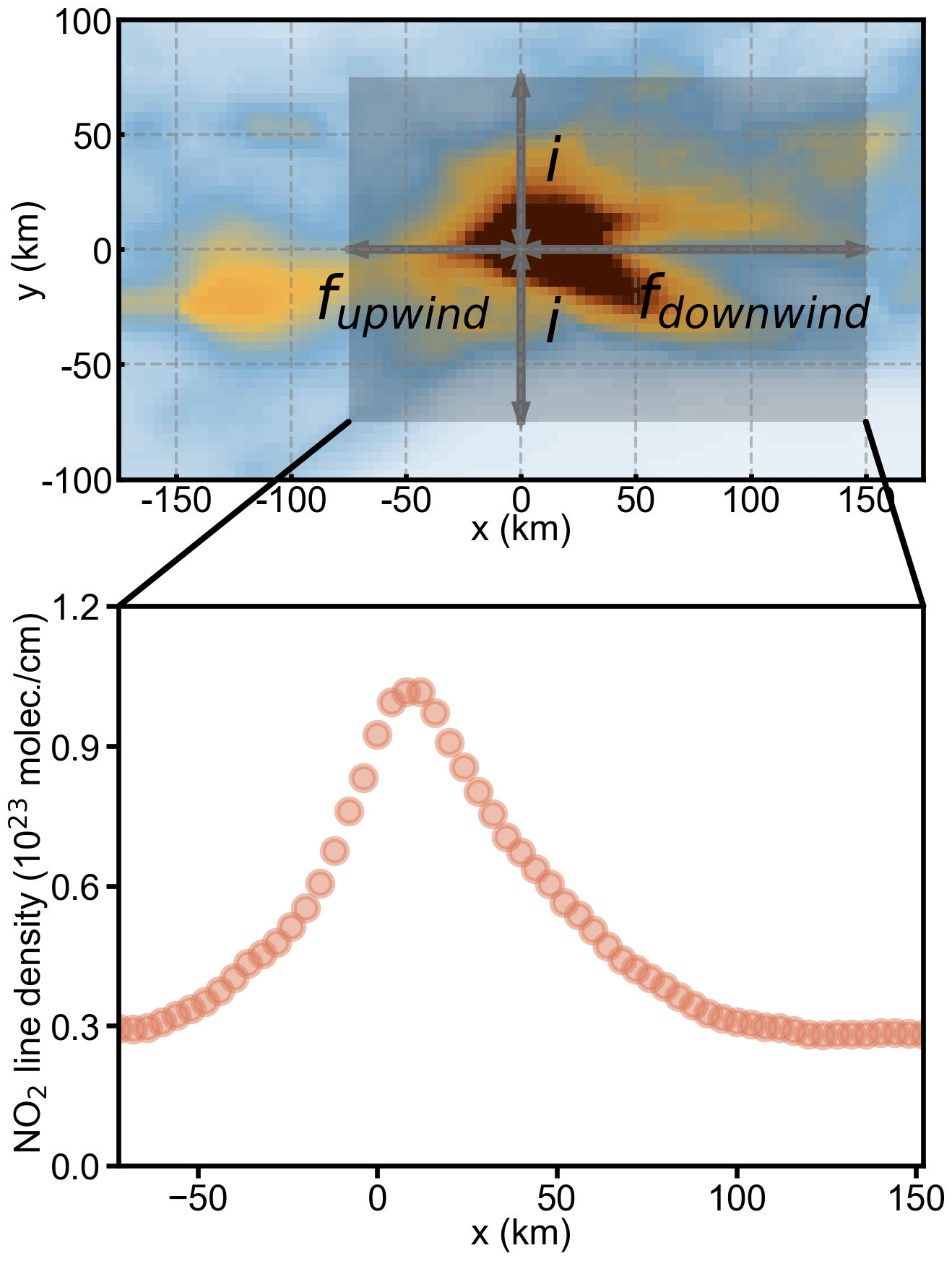
Figure 3 Sketch of the definition of line densities. For each wind direction, mean NO₂ VCDs are integrated in across-wind direction y over the interval i, resulting in line densities LD(x). The fit is performed over the entire upwind interval (f_upwind) and downwind interval (f_downwind). The city center is the coordinate origin. The top panel shows the NU-WRF tropospheric NO₂ VCDs around New York City under southwesterly wind; however the image is rotated by 45^∘ in the clockwise direction to present NO₂ VCDs in an upwind–downwind direction. The city of Philadelphia and Long Island are located in the upwind and downwind direction, respectively.

We then use the following model function, f(x), to describe NO₂ line densities under windy conditions (wind speed > 2 m s⁻¹) LD_windy(x):

$$\begin{array}{}\text{(2)}& \begin{array}{rl}f\left(x\right)& ={\displaystyle \frac{E\left(x\right)}{R_{{\mathrm{NO}}_{\mathit{\text{x}}}:{\mathrm{NO}}_{\mathrm{2}}}\cdot w}}\ast e^{-\frac{x}{w\cdot \mathit{\tau }}}+b\\ & ={\displaystyle \frac{\left[{\text{LD}}_{\text{calm}}\right(x)-b]}{\mathit{\tau }\cdot w}}\ast e^{-\frac{x}{w\cdot \mathit{\tau }}}+b,\end{array}\end{array}$$

where w is the mean wind speed at the emission level in a given direction x, and ∗ denotes convolution. Figure 3 illustrates the calculation of LD_windy(x). Additional technical details of the model function f(x) and its differences compared to those proposed by Liu et al. (2016b) are given in Appendix A.

Finally, we use estimates of b and $R_{{\mathrm{NO}}_{\mathit{\text{x}}}:{\mathrm{NO}}_{\mathrm{2}}}$ in Eq. (2), along with values of w, LD_calm(x), and LD_windy(x) from the model simulation to infer τ and E(x). As displayed in Fig. 1, we use the NU-WRF high-resolution tropospheric NO₂ VCDs sampled at 14:00 LT as the synthetic NO₂ VCD observations, together with the NU-WRF meteorological wind information, to estimate urban NO_x emissions. In other words, here we assume perfect knowledge of the winds and do not further consider the impact of errors in w. As in previous studies, we only analyze data from April to September, in order to exclude winter data that have larger uncertainties and longer NO_x lifetimes. We also investigate the impact of the inclusion of winter data in Sect. 3.3.1; it is found to be associated with a larger uncertainty. We further compute total emissions for each city, ${\text{Emis}}_{{\mathrm{NO}}_{\mathit{\text{x}}}}$, by summing E(x).

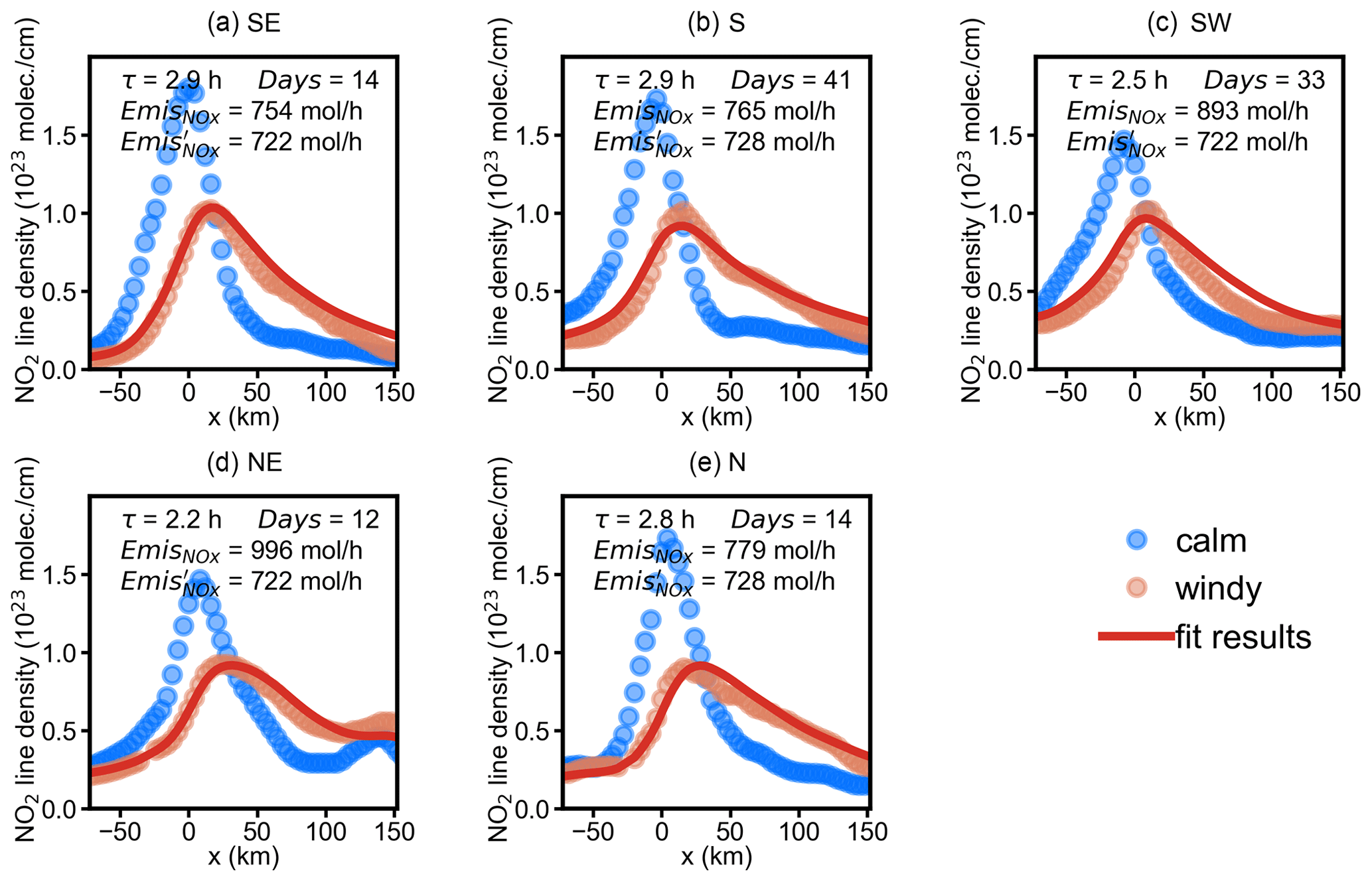
Figure 4 NO₂ line densities around New York for different wind direction sectors. Circles: NO₂ line densities for calm (blue circles) and (a) southeasterly, (b) southerly, (c) southwesterly, (d) northeasterly, and (e) northerly winds (red circles) as a function of the distance x to the center of New York. Red line: the fit result f(x). The numbers indicate the fitted NO_x lifetime (τ), average days of data used for calculating NO₂ line densities (days), derived emissions (${\text{Emis}}_{{\mathrm{NO}}_{\mathit{\text{x}}}}$), and given emissions (${\text{Emis}}_{{\mathrm{NO}}_{\mathit{\text{x}}}}^{\prime }$). NO₂ line densities are derived from NO₂ VCDs averaged from April through September 2016. NO₂ line densities for the remaining wind direction sectors are discarded due to the fitting results having insufficient quality.

We perform a nonlinear least-squares fit of f(x) to the observed line densities under windy conditions, LD_windy(x), with τ as the single fitting parameter. We use the package of scipy.optimize.curve_fit from the Python software library to perform the fitting. We set the fit interval to 150 km in the downwind direction, which corresponds to the e-folding distance for τ = 6 h and w = 7 m s⁻¹. The fit intervals in the upwind direction and the y direction are set to half the e-folding distance (75 km); the resulting area is large enough to cover a highly populated and spread-out metropolitan region such as New York City. The definitions of the fit interval in the upwind and downwind direction and the across-wind integration interval are illustrated in Fig. 3. Note that we use LD_calm(x) over a larger horizontal interval of 450 km to calculate the convolution in Eq. (2), in order to eliminate the edge effect of convolution. Fitting results of insufficient quality (i.e., the correlation coefficient R between the fitted and observed NO₂ LD < 0.9 and 1 standard deviation error of τ > 10 %) are discarded. We infer emissions simultaneously by summing E(x) in Eq. (1). We perform the fit for all wind direction sectors and then average the fitted τ and corresponding total emission ${\text{Emis}}_{{\mathrm{NO}}_{\mathit{\text{x}}}}$ with good quality, using the fit residuals as inverse weights, to yield a best estimate of 〈τ〉 and $\langle {\text{Emis}}_{{\mathrm{NO}}_{\mathit{\text{x}}}}\rangle$ for a given city. The standard deviation of the fit results for different wind directions has been used to quantify uncertainties in Sect. 3.3.2.

We use the city of New York as a case study to demonstrate our approach. This city is well suited for illustrating the strength of MISATEAM to estimate emissions for mixed sources because it is a large city with multiple point and areal sources and is surrounded by many other large sources. Figure 3 displays the complex spatial distribution of sources around New York. Under southwesterly wind, the city of Philadelphia is located in the upwind direction, and Long Island is located in the downwind direction, both of which are significant NO_x sources. Note that we do not exclude cloudy days from our analysis to make the most of the NU-WRF NO₂ simulations and to avoid additional uncertainties arising from the inconsistent definitions of cloud fractions in the NU-WRF and satellite NO₂ products. The uncertainty of the presence of clouds is discussed in Sect. 3.3.2.

We use wind fields averaged from the surface to 1000 m altitude for w in this study. The synthetic NO₂ VCDs around New York are sorted by wind direction (Fig. S1). Figure 4a displays the observed line densities for calm (blue circles) and southeasterly winds (red circles) around New York and the fitted model function f(x) (red lines). Generally, f(x) describes the observed downwind patterns very well; the coefficients of determination (R²) between observation and fit are 0.90–0.98 for different wind directions. The resulting lifetimes show a range of 2.2–2.9 h, which result in emissions of 754–996 mol h⁻¹ for different wind directions, as shown in Fig. 4a–e. Results for other wind direction sectors are discarded due to the fitting results being of insufficient quality (westerly and northwesterly winds; Fig. S2 in the Supplement) or a lack of observations (easterly wind).

2.3 Impact of temporal variations in wind fields

CTM-independent emission estimation algorithms usually assume a steady wind field over the duration of NO_x lifetime. In the demonstration in Sect. 2.2, we use the wind fields sampled at the satellite overpass time to drive MISATEAM, consistent with previous studies (e.g., Beirle et al., 2011; Valin et al., 2013; Lu et al., 2015; Liu et al., 2017, 2020; Goldberg et al., 2019). This is expected to be reasonable for species with a short lifetime of a few hours such as NO_x near noon of non-winter seasons. In reality, wind fields are variable over the NO_x lifetime. Consequently, NO_x emitted at a time prior to the satellite overpass may be transported under different wind conditions than those at the overpass time.

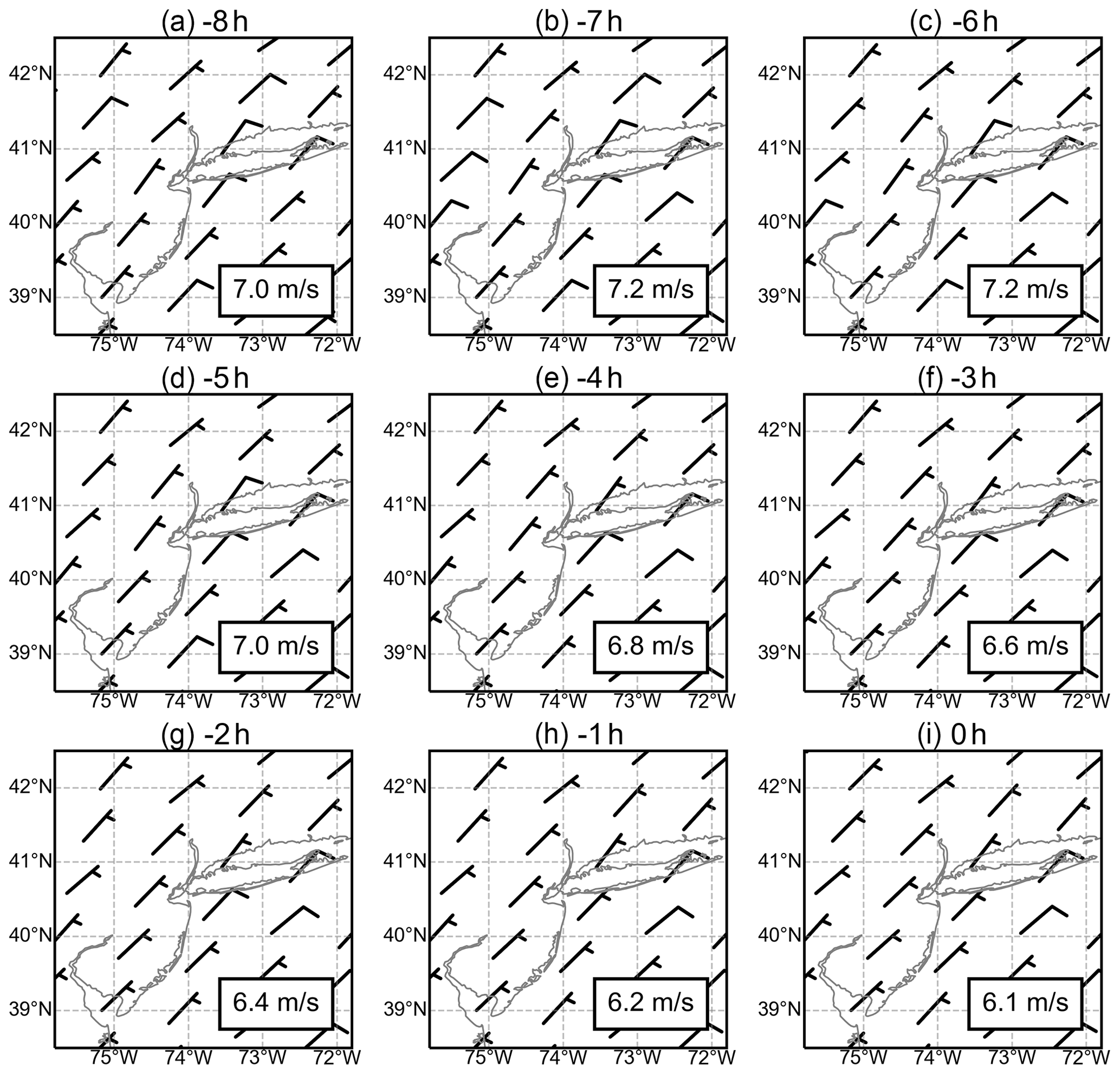
Figure 5 Wind barbs around New York City for different times of the day. All northeasterly winds at 14:00 LT from April to September of 2016 are averaged and shown in (i). Wind barbs for the northeasterly winds backward trajectories from 8 to 1 h prior to 14:00 LT are displayed in (a–h). Wind speed is given in units of knots, which is equivalent to nautical miles per hour (1.9 km h⁻¹). Each short and long barb represents 5 knots (9.3 km h⁻¹) and 10 knots (18.5 km h⁻¹), respectively. The average wind speed is displayed in the grey box.

Figure 5 illustrates the temporal variations in wind fields around New York. We use the northeasterly wind direction (with a good fitting result) for demonstration. We select northeasterly winds observed at 14:00 LT as the baseline and find their backward trajectories for up to 8 h. The backward trajectories are given at a time step of 1 h. Not surprisingly, winds are not constant during the 9 h from 8 h before the baseline to the exact hour of the baseline. However, the temporal variations in wind directions are rather small for the northeasterly wind; wind directions are almost constant over time. For wind directions without good fit results, we observe larger variations. For instance, for the westerly wind with a poor correlation coefficient R of 0.76, the wind directions deviate from the west direction gradually for the time prior to the baseline (Fig. S3 in the Supplement). These results shed light on the robustness of MISATEAM's steady-wind assumption. It is most likely that the fit fails when the assumption of steady wind is not satisfied. In other words, the inherent fitting assumption is robust when the fit results have sufficient quality as defined in Sect. 2.2.

We perform sensitivity analyses to investigate the potential impact of temporal variations in winds on the fit results. We extend the time windows used for calculating averaged wind fields from 1 h (i.e., at the overpass time of 14:00 LT) to 3 h (i.e., starting from the overpass time and extending into the past 2 h), 6, 9, and 12 h. We weight the winds based on their temporal proximity; i.e., the wind closer to the overpass time is given larger weight, following Eq. (3).

$$\begin{array}{}\text{(3)}& \stackrel{\mathrm{‾}}{w_{i,d}}={\displaystyle \frac{{\sum }_{h=\mathrm{0}}^N{w}_{h,i,d}\cdot e^{-h/t\mathrm{0}}}{{\sum }_{h=\mathrm{0}}^N{e}^{-h/t\mathrm{0}}}},\end{array}$$

where h represents the number of hours prior to the overpass time. i and d denote an individual grid cell and day, respectively. $w_{h,i,d}$ is the wind for a specific grid cell i on day d at the time of h hours prior to the overpass time. N is the length of the time window used (units of hour). The weighted average winds $\stackrel{\mathrm{‾}}{w_{i,d}}$ are further applied with MISATEAM to infer NO_x lifetimes and emissions for investigated cities. We set t₀ to a constant value of 3 derived from rounding the average NU-WRF lifetimes for all investigated cities (see details in Sect. 2.4). The fitting results are found to be relatively insensitive to the choice of t₀. The differences of the fitted lifetimes and emissions are −2 ± 15 % and 3 ± 16 %, respectively, when we increase t₀ by a factor of 2. This is significantly smaller than the difference between the fit results based on weighted average winds and the winds at the overpass time (shown in Sect. 3.1).

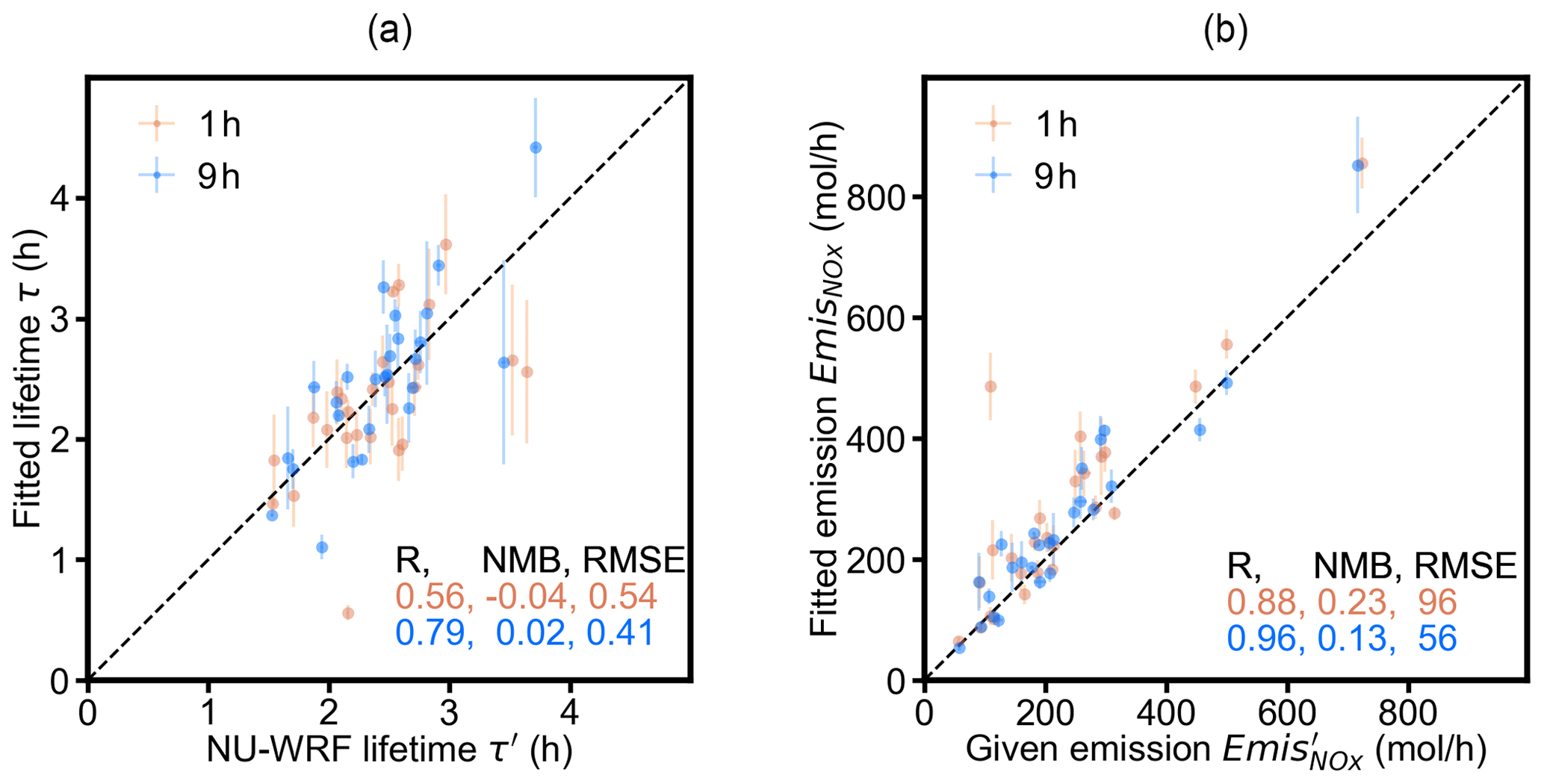
Figure 6 Scatterplots of (a) the fitted NO_x lifetime τ as compared to the NU-WRF lifetime τ^′ and (b) the fitted NO_x emissions ${\text{Emis}}_{{\mathrm{NO}}_{\mathit{\text{x}}}}$ as compared to the given emissions ${\text{Emis}}_{{\mathrm{NO}}_{\mathit{\text{x}}}}^{\prime }$. Error bars show the standard error of the fitted results for all available wind directions. Standard error is defined as standard deviation divided by $\sqrt{n}$, with n being the number of available wind directions. The results deriving from the wind fields sampled at 14:00 LT (“1 h”) and the weighted average of 9 h wind fields (“9 h”) are displayed by red and blue dots, respectively. The dashed line represents the 1:1 line.

2.4 Performance evaluation

In order to evaluate the fitting results, we infer given emissions and NU-WRF lifetimes from the NU-WRF inputs/outputs. The given emission ${\text{Emis}}_{{\mathrm{NO}}_{\mathit{\text{x}}}}^{\prime }$ is derived by summing NU-WRF NO_x emissions from all grid cells within the fit interval. The NU-WRF lifetime τ^′ can be computed by solving Eq. (1); i.e.,

$$\begin{array}{}\text{(4)}& {\mathit{\tau }}^{\prime }={\displaystyle \frac{\sum R_{{\mathrm{NO}}_{\mathit{\text{x}}}:{\mathrm{NO}}_{\mathrm{2}}}\cdot \left[{\text{LD}}_{\text{calm}}\right(x)-b]}{\sum E^{\prime }\left(x\right)}},\end{array}$$

where E^′(x) is the given NO_x emission line densities under calm wind conditions, as a function of distance x from the city center. For evaluation, we compute the correlation coefficient (R), the normalized mean bias (NMB), and the root mean squared error (RMSE) of the fitted emissions and the given emissions for all investigated cities. The model performance metrics of NMB and RMSE for the emission (${\text{Emis}}_{{\mathrm{NO}}_{\mathit{\text{x}}}}$) evaluation are defined as

$$\begin{array}{}\text{(5)}& \mathrm{NMB}={\displaystyle \frac{{\sum }_{i=\mathrm{1}}^n({\text{Emis}}_{{\mathrm{NO}}_{\mathit{\text{x}}},i}-{\text{Emis}}_{{\mathrm{NO}}_{\mathit{\text{x}}},i}^{\prime })}{{\sum }_{i=\mathrm{1}}^n{\text{Emis}}_{{\mathrm{NO}}_{\mathit{\text{x}}},i}^{\prime }}}\end{array}$$

and

$$\begin{array}{}\text{(6)}& \text{RMSE}=\sqrt{{\displaystyle \frac{{\sum }_{i=\mathrm{1}}^n({\text{Emis}}_{{\mathrm{NO}}_{\mathit{\text{x}}},i}-{\text{Emis}}_{{\mathrm{NO}}_{\mathit{\text{x}}},i}^{\prime }{)}^{\mathrm{2}}}{n}}}\end{array}$$

respectively, where i represents the individual city, and n is the total number of cities used for evaluation. The metrics for lifetime evaluation are consistent with Eqs. (5) and (6) when replacing ${\text{Emis}}_{{\mathrm{NO}}_{\mathit{\text{x}}}}$ with τ and ${\text{Emis}}_{{\mathrm{NO}}_{\mathit{\text{x}}}}^{\prime }$ with τ^′. A good method should have a large R, a near-zero NMB, and a small RMSE.

3 Results and discussion

3.1 Evaluation

We apply MISATEAM to 60 large cities over the United States (see the selection criteria of cities in Sect. 2.1). For five cities, we are not able to initiate the fitting procedure, due to a lack of observations under calm wind conditions to calculate LD_calm(x). We derive valid fitting results for 26 cities. The locations of the 26 cities are shown in Fig. 2. The other 29 cities without valid results either had small correlation coefficients (< 0.9) or large fitting errors (standard deviation error of τ > 10 %); those cities tend to have larger temporal variations in winds (similar to Fig. S3), which do not satisfy MISATEAM's requirement for steady winds prior to the satellite overpass.

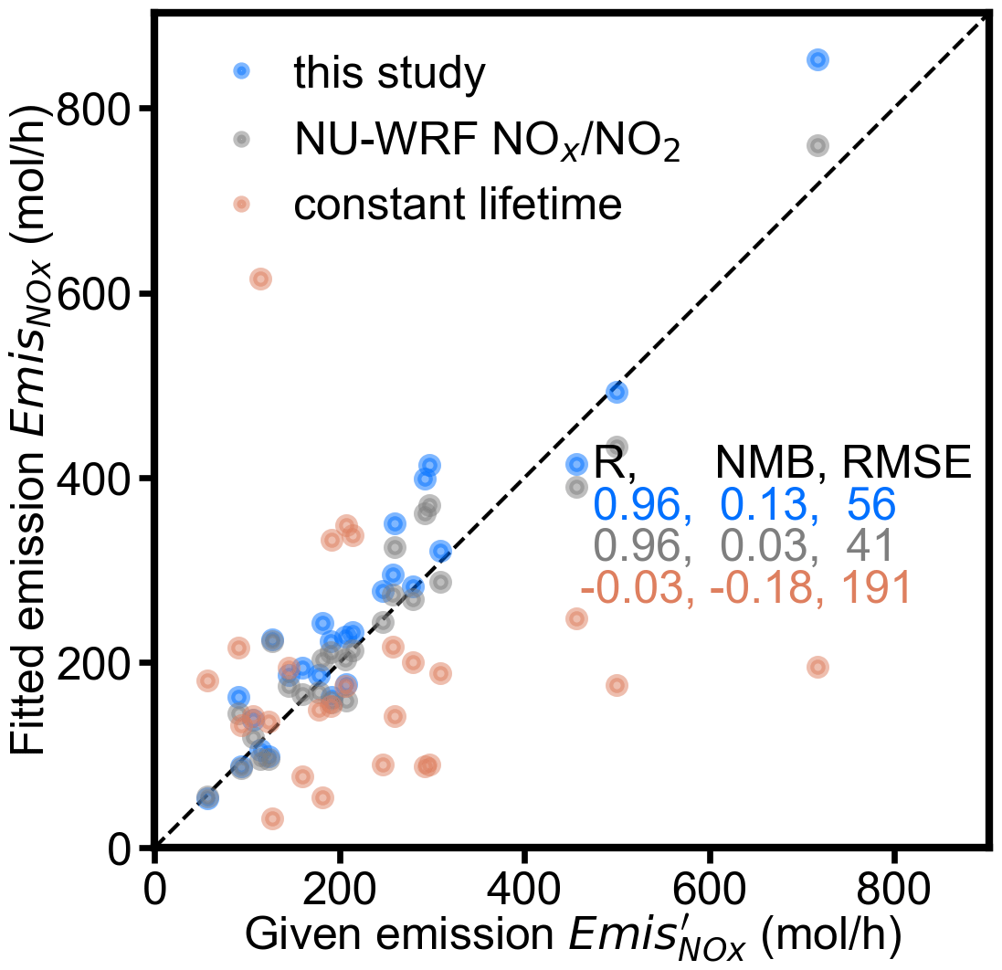
Figure 7 Scatterplot of the fitted total NO_x emissions ${\text{Emis}}_{{\mathrm{NO}}_{\mathit{\text{x}}}}$ as compared to the given total emissions ${\text{Emis}}_{{\mathrm{NO}}_{\mathit{\text{x}}}}^{\prime }$ under different scenarios. The blue, grey, and red dots represent the scenarios based on the fitted lifetime τ and a constant NO_x to NO₂ ratio of 1.32 (“this study”), the fitted lifetime τ and the NO_x to NO₂ ratio given by the NU-WRF model (“NU-WRF ${\mathrm{NO}}_{\mathit{\text{x}}}/{\mathrm{NO}}_{\mathrm{2}}$”), and a constant lifetime of 2.5 h and a constant NO_x to NO₂ ratio of 1.32 (“constant lifetime”), respectively. The dashed line represents the 1:1 line. Statistics are provided in the inset table.

Figure 6 compares MISATEAM estimated lifetimes and emissions with the NU-WRF lifetimes and given emissions for the 26 cities. The comparison shows good consistency in general. For results derived from the wind data sampled at the overpass time (hereafter referred to as “1 h wind”; red dots), values of R are 0.56 and 0.88 for lifetimes and emissions, respectively. The bias is rather small for the lifetime comparison with NMB of −0.04 and RMSE of 0.54. The bias is larger for emissions, primarily caused by the assumption of a constant NO_x to NO₂ ratio ($R_{{\mathrm{NO}}_{\mathit{\text{x}}}:{\mathrm{NO}}_{\mathrm{2}}}$). The errors arising from the differences between $R_{{\mathrm{NO}}_{\mathit{\text{x}}}:{\mathrm{NO}}_{\mathrm{2}}}$ for individual cities and a constant value of 1.32 will be propagated into the resulting emissions. The impact of the prescribed $R_{{\mathrm{NO}}_{\mathit{\text{x}}}:{\mathrm{NO}}_{\mathrm{2}}}$ on inferring emissions will be discussed in more detail in this section (Fig. 7).

The use of wind data over 9 h prior to the overpass time improves the performance of MISATEAM. Figure 6 compares the inferred lifetimes and emissions based on the 9 h weighted average of wind data (hereafter referred to as “9 h wind”; blue dots). The results derived from the weighted average wind data show larger correlations with R increasing from 0.56 to 0.79 for lifetimes and from 0.88 to 0.96 for emissions and a smaller bias with NMB decreasing from −0.04 to 0.02 for lifetimes and from 0.23 to 0.13 for emissions, when comparing with results derived from the 1 h wind. We have performed the comparison using results based on the weighted averages of 3, 6, and 12 h wind data as well. The use of wind information prior to the satellite overpass time succeeds in improving the performance of MISATEAM in all these cases (Fig. S4 in the Supplement). Note that the correlation between the inferred and the NU-WRF lifetimes based on 12 h wind (R= 0.64) is not as good as that based on 3 h (R= 0.74), 6 h (R= 0.78), and 9 h (R= 0.79) wind, which is most likely caused by the inclusion of overnight wind information.

The importance of applying wind information prior to the satellite overpass time should not be overinterpreted. The fitting function Eq. (2) by definition is not capable of describing the NO₂ plumes under significantly varying wind directions because such temporal variations are not considered in the fitting function. In this way, wind directions and the results inferred from different wind scenarios are not expected to vary significantly, as far as fits with sufficient quality are yielded. Only 6 out of 26 cities show relative differences larger than 20 % when comparing results derived from 1 h wind to those derived from 9 h wind.

We examine a scenario, namely “NU-WRF ${\mathrm{NO}}_{\mathit{\text{x}}}/{\mathrm{NO}}_{\mathrm{2}}$”, to investigate possible errors from the assumption of a constant $R_{{\mathrm{NO}}_{\mathit{\text{x}}}:{\mathrm{NO}}_{\mathrm{2}}}$. We replace $R_{{\mathrm{NO}}_{\mathit{\text{x}}}:{\mathrm{NO}}_{\mathrm{2}}}$ with the ratio of NO_x and NO₂ calculated directly from NO₂ and NO VCDs per grid cell by NU-WRF outputs and then use MISATEAM for inferring NO_x emissions. Any difference in the inferred emissions compared to the emissions based on the prescribed ratio of 1.32 (“this study”) can then be assumed to originate from errors in the assumption of $R_{{\mathrm{NO}}_{\mathit{\text{x}}}:{\mathrm{NO}}_{\mathrm{2}}}$. Figure 7 compares the results using a prescribed ratio (blue dots) with those using NU-WRF ${\mathrm{NO}}_{\mathit{\text{x}}}/{\mathrm{NO}}_{\mathrm{2}}$ (grey dots). The comparison shows nearly the same correlations to the given emissions but a smaller bias for results based on NU-WRF ${\mathrm{NO}}_{\mathit{\text{x}}}/{\mathrm{NO}}_{\mathrm{2}}$, with NMB dropping from 0.13 to almost zero (0.03). The comparison suggests that the influence of changing ratio on derived emissions is limited because its spatial variation is significantly smaller than that of NO_x lifetime and NO₂ columns (τ and LD_calm(x) in Eq. 1). Considering the investigated cities are located all over the country and have a wide range of geographic features, we conclude that a constant ratio is a reasonable assumption without resulting in significant bias to the derived emissions for typical US cities. The error associated with the assumption is estimated to be 10 %, consistent with our previous estimates based on literature reviews (Beirle et al., 2011; Liu et al., 2016b). However, for applications based on geostationary satellites with changing local observation time, the approach using a constant value for $R_{{\mathrm{NO}}_{\mathit{\text{x}}}:{\mathrm{NO}}_{\mathrm{2}}}$ is subject to larger uncertainties arising from the diurnal cycle of $R_{{\mathrm{NO}}_{\mathit{\text{x}}}:{\mathrm{NO}}_{\mathrm{2}}}$(Han et al., 2011).

We examine an additional scenario, namely “constant lifetime”, to show the necessity of deriving lifetimes for individual cities. Instead of individually fitted lifetimes for each city, we use the mean NU-WRF lifetime of all cities (2.5 h) for the calculation of emissions in the constant lifetime scenario. The emissions correlation drops to −0.03 (Fig. 7), showing that individually fitted lifetimes are critical for this method. The bias is also larger, with RMSE increasing by a factor of 3 compared to results based on the individually fitted lifetimes. This further improves our confidence that the derived variation of the fitted lifetimes carries important information on local variability of the oxidizing capacity of urban plumes. The individual lifetimes are well suited for the determination of emissions, suggested by the significantly improved consistency with given emissions.

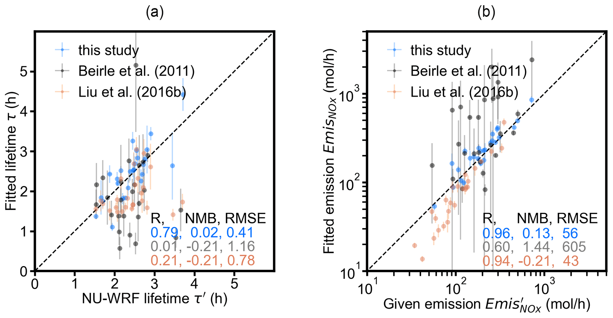
Figure 8 Scatterplots of (a) the fitted NO_x lifetime τ as compared to the NU-WRF lifetime τ^′ and (b) the fitted NO_x emissions ${\text{Emis}}_{{\mathrm{NO}}_{\mathit{\text{x}}}}$ as compared to the given emissions ${\text{Emis}}_{{\mathrm{NO}}_{\mathit{\text{x}}}}^{\prime }$. Error bars show the standard error of the fitted results for all available wind directions. Standard error is defined as standard deviation divided by $\sqrt{n}$, with n being the number of available wind directions. The results derived from MISATEAM, the approach of Beirle et al. (2011), and the approach of Liu et al. (2016b) are displayed by blue, grey, and red dots, respectively. The dashed line represents the 1:1 line. Note that (b) is plotted on a logarithmic scale.

3.2 Comparison with previous methods

We further evaluate MISATEAM by comparing the results with those derived from two previous approaches, including Beirle et al. (2011) and Liu et al. (2016b). The comparison of the technical details between MISATEAM and these two previous approaches is given by Fig. S5 in the Supplement. We apply all three approaches to fit lifetimes and emissions for all 26 cities investigated by this study. Note that we use the 9 h wind for all approaches for best performance and consistency.

Figure 8a illustrates the comparison for inferring lifetimes. The approach of Beirle et al. (2011) does not predict lifetimes well, with a poor correlation (R= 0.01). The correlation improves (R= 0.36) when eliminating the data for seven cities with large (> 5 h) or small (< 1 h) fitted lifetimes, assuming the NO_x emission distributions around these cities do not meet the requirements of the Beirle et al. method. The poor correlation is not surprising because by definition the method can only represent a single-point source convolved with a Gaussian function and was not intended to be applied to mixed sources with interfering emissions from nearby cities or industrial areas. For instance, it is capable of giving an accurate estimate for the isolated city of St. Louis in Missouri, with a relative difference of less than 10 % compared to the NU-WRF lifetime. However, for most cities with a polluted background, the fitted lifetimes are biased significantly due to the interference from surroundings. This is consistent with the previous findings for this approach: an additional source at 100 km with only 10 % of the emissions of the source under investigation causes a lifetime bias of 20 %; for an interfering source of the same order as the source of interest, the method fails completely (Liu et al., 2016b). Several studies adopted a plume rotation technique (Pommier et al., 2013; Valin et al., 2013) to advance the approach of Beirle et al. (2011), which is not applicable to mixed sources as well. These techniques rotate NO₂ measurements centered over the city center so that NO₂ columns under different wind directions are aligned in a common upwind-to-downwind direction. This increases the number of observations used for analysis without introducing additional errors for (quasi) point sources, compared with individually analyzing observations by wind directions as done in this study. However, for mixed sources investigated in this study, the use of such rotation techniques may result in significant bias by allocating the NO₂ from interfering sources into a ring of elevated NO₂ values around the source of the interest and thus amplifying the NO₂ signal of the source. An illustration of this amplification can be found in Fig. S2 of Fioletov et al. (2015).

We note that the performance of MISATEAM is also better than that of the approach reported in Liu et al. (2016b), although they share the same concept of using the NO₂ patterns observed under calm wind conditions as a proxy for emission patterns instead of assuming a single-point source as in Beirle et al. (2011). It is most likely that Liu et al. (2016b) overfit the model by introducing too many degrees of freedom. As suggested by Fig. 8a, the model function of Liu et al. (2016b) occasionally tries to “explain” changes of scaling factors by a shorter lifetime, resulting in a small R of 0.21. In MISATEAM, we decrease the number of fitting parameters from three in Liu et al. (2016b) to only one (see details in Eq. A4 of Appendix A), which improves the robustness of the fit results.

Table 1 The mean relative change of lifetimes and emissions for different choices of fit and integration intervals and wind fields.

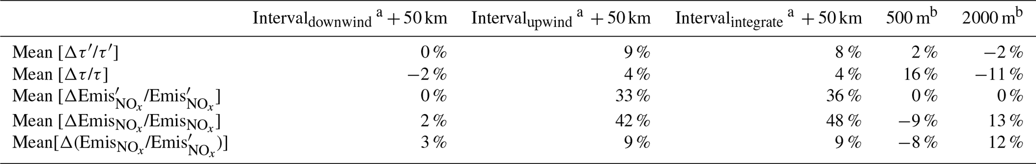
^a Interval_downwind = 150 km. Interval_upwind = 75 km. Interval_integrate = 150 km. ^b The wind fields are averaged from the surface up to this height.

Emission comparisons in Fig. 8b show better agreement than lifetime comparisons in Fig. 8a for all approaches. MISATEAM-derived emissions show the best consistency with the given emissions. According to mass balance, the magnitude of emissions equals the total mass of NO_x divided by lifetime. In the evaluation for MISATEAM, the given emissions range from 57 to 717 mol h⁻¹ for all investigated cities, the variation in which is significantly larger than that in lifetimes ranging from 1.5 to 3.7 h. This finding also holds for the other two approaches. The other two approaches can achieve a good correlation with the given emissions by providing reasonable estimates for the magnitude of the total NO_x mass, even though they fail to predict variations in lifetimes between cities. For instance, the results derived from the approach of Liu et al. (2016b) show a small R of 0.21 to the NU-WRF lifetimes but a significantly stronger correlation to the given emissions of 0.94, which is comparable to that of MISATEAM-derived emissions. But Liu et al. (2016b)-derived emissions are still associated with larger biases arising from the estimates for lifetimes. The values of NMB are 0.13 and −0.21 for emissions derived from MISATEAM and the approach of Liu et al. (2016b), respectively, when comparing against the given emissions. Note that the derived and given emissions from the approach of Liu et al. (2016b) are smaller than the two other approaches but do not indicate a smaller bias. Liu et al. (2016b) only aim to estimate emissions from the city center, considered as a (quasi) point source, instead of all sources in the urban area. In this way, ${\text{Emis}}_{{\mathrm{NO}}_{\mathit{\text{x}}}}$ and ${\text{Emis}}_{{\mathrm{NO}}_{\mathit{\text{x}}}}^{\prime }$, and thus RMSE, are smaller than those for MISATEAM.

3.3 Uncertainty analysis

The good consistency in Sect. 3.1 increases our confidence that the fitted lifetimes and emissions represent the real-world characteristics well. We investigate their uncertainties in this section.

3.3.1 Sensitivity analysis

Analogous to Beirle et al. (2011) and Liu et al. (2016b), we investigate the impact of the a priori choice of fit and integration intervals and wind layer height. The dependency of the fit results for τ and ${\text{Emis}}_{{\mathrm{NO}}_{\mathit{\text{x}}}}$ on these three choices is tabulated in Table 1.

The fitted lifetimes are generally robust with respect to changes of the fit and integration intervals because the NO₂ distribution under calm wind conditions, LD_calm(x), is a good representation of the emission pattern in any case. An increase of the fit interval in the downwind direction by 50 km affects the resulting lifetimes by about −2 ± 11 %. The changes of derived lifetimes are also small when increasing the fit interval in the upwind direction (4 ± 12 %) or the integration interval (interval i + 25 km in Fig. 3; 4 ± 18 %) by 50 km. MISATEAM succeeds in avoiding choosing intervals city by city manually, which has been done in previous studies in order to minimize the influence of other nearby sources.

We use the change of the ratio of fitted emissions ${\text{Emis}}_{{\mathrm{NO}}_{\mathit{\text{x}}}}$ to given emissions ${\text{Emis}}_{{\mathrm{NO}}_{\mathit{\text{x}}}}^{\prime }$, $\mathrm{\Delta }({\text{Emis}}_{{\mathrm{NO}}_{\mathit{\text{x}}}}/{\text{Emis}}_{{\mathrm{NO}}_{\mathit{\text{x}}}}^{\prime }$), to show the impact of the enlarged fit and integration intervals on emissions. We do not focus on the change of emissions, $\mathrm{\Delta }{\text{Emis}}_{{\mathrm{NO}}_{\mathit{\text{x}}}}/{\text{Emis}}_{{\mathrm{NO}}_{\mathit{\text{x}}}}$ because the fitted emissions are expected to be sensitive to the enlarged intervals, which include additional sources and thus more emissions. The fitted emissions show an average growth of 48 % associated with extending the integration interval by 50 km to increase the given emissions by 36 %. The rise in emissions is similar to increasing the fit interval in the upwind direction by 50 km with 33 % for the given emissions and 42 % for the fitted emissions. However, for the scenario of a larger downwind-direction, upwind-direction, and integration interval, the change of the ratio of ${\text{Emis}}_{{\mathrm{NO}}_{\mathit{\text{x}}}}$ to ${\text{Emis}}_{{\mathrm{NO}}_{\mathit{\text{x}}}}^{\prime }$ is rather small, which is 3 %, 9 %, and 9 % on average, respectively; the fitted emissions show good consistency with the given emissions, reporting correlation coefficients of 0.95, 0.92, and 0.86, respectively. It is interesting to note that the fitted emissions are rather insensitive to the extension of the fit interval in downwind direction. Neither the given nor the fitted emissions are significantly changed by increasing the downwind-direction interval from 150 to 200 km. It suggests that we succeed in capturing the complete downwind plume and reaching the background areas by the default setting of 150 km for the investigated cities in this study.

Uncertainties associated with the choice of top wind layer height (e.g., 500, 1000, or 2000 m) are relatively small. The resulting lifetimes and emissions change about 16 % and −9 % on average when averaging the wind fields from the surface to up to 500 m. The average changes are −11 % and 13 % for inferring lifetimes and emissions, respectively, when adopting the wind layer height of 2000 m. This is consistent with the findings in the previous studies (e.g., Beirle et al., 2011 and Liu et al., 2016b).

We also apply MISATEAM to year-round NO₂ data to investigate the impact of including winter data on the performance of the method. We keep default settings of MISATEAM as described in Sect. 2.2 for the fit. As expected, the fitted results differ more significantly from given values compared with results based on using only non-winter data. The bias is larger with NMB changing from 0.02 to −0.14 for lifetimes and from 0.13 to 0.27 for emissions. This indicates that MISATEAM, most likely its inherent steady-wind assumption, is less accurate during the winter season with longer NO_x lifetimes.

3.3.2 Uncertainty quantification

We calculate the uncertainties of inferred results based on the fitting metrics (Figs. 6 and 7) and the dependencies on the a priori settings as investigated in the above sensitivity studies. We attribute uncertainties of 15 % and 20 % to the derived lifetimes and emissions, respectively, based on the mean of relative differences for all 26 cities (14 % for lifetimes and 21 % for emissions). The derived emissions have higher uncertainties arising from uncertainty in the NO_x to NO₂ scaling factor. The derived emissions in terms of NO₂ are upscaled to NO_x based on a constant ${\mathrm{NO}}_{\mathit{\text{x}}}/{\mathrm{NO}}_{\mathrm{2}}$ ratio of 1.32, representing typical urban conditions at noon (Seinfeld and Pandis, 2006). Since MISATEAM aims to provide estimates for cloud-free satellite observations at the overpass time close to noon of non-winter seasons, and it focuses on polluted regions with generally high tropospheric ozone, this value is reasonably accurate. However, the ${\mathrm{NO}}_{\mathit{\text{x}}}/{\mathrm{NO}}_{\mathrm{2}}$ ratio might vary locally. NU-WRF reports 1.4 ± 0.1 with a range of 1.2–1.6. The overall impact of variations in this ratio is shown to be relatively small (see Sect. 3.1).

We can identify additional uncertainties that would be present when applying MISATEAM to “real” data instead of synthetic data. The uncertainty of satellite NO₂ observations propagates into the uncertainty of emissions. The uncertainty of satellite NO₂ observations has less impact on the lifetime estimation and only results in errors for lifetimes when satellite observations have systematic errors depending on the distance from the source. The total uncertainty of NO₂ VCDs results from uncertainties in the spectral fit in the retrieval, the stratospheric and tropospheric separation, and the tropospheric air mass factor (AMF). In the model function of MISATEAM, a possible bias associated with the stratospheric and tropospheric separation is eliminated by use of the background term b. The uncertainty in the spectral fit in the retrieval is rather small compared to that associated with AMF (Boersma et al., 2007). We estimated the overall uncertainty primarily arising from the uncertainty in the tropospheric AMF is about 25 % based on validation of TROPOMI NO₂ products with ground-based measurements (e.g., Griffin et al., 2019; Ialongo et al., 2020; Zhao et al., 2020). Since the random uncertainty of the tropospheric NO₂ observations could be suppressed due to the consideration of long-term means, this estimate may be conservative.

The presence of clouds is an additional source of uncertainties. We are required to exclude satellite observations with significant cloud fractions in the instrument's field of view. For TROPOMI NO₂ products, we usually remove data with cloud radiance fraction ≥ 0.5. A bias is observed in NO₂ VCD averages as a result of removing the data during cloudy conditions (Geddes et al., 2012). The bias is associated with changing photochemistry, meteorology, and pollutant transport, which may also have impacts on the ${\mathrm{NO}}_{\mathit{\text{x}}}/{\mathrm{NO}}_{\mathrm{2}}$ ratio and NO_x lifetime. NO_x lifetime on a sunny day with valid satellite observations will likely be shorter than that on a cloudy day since faster photolysis rates are expected for NO_x reactions on sunny days. The magnitude of a bias is expected to vary from city to city. We calculate the fraction of cloudy scenes to total scenes over the fit domain of individual cities based on TROPOMI NO₂ products from April through September, 2020. The fractions range from 16 %–56 % for the considered cities. For cities with heavy cloud cover, like New York, Philadelphia, and Washington D.C., with a fraction > 50 %, the impact associated with cloud selection criteria is expected to be larger than cities with more clear sky. We estimated an uncertainty of 10 % arising from cloud selection criteria based on the evaluation performed at urban sites (Geddes et al., 2012).

Additionally, the accuracy of wind fields contributes to the uncertainties of both lifetimes and emissions. It can affect the sorting of the NO₂ VCDs according to wind direction as well as the conversion of the downwind decay from a function of distance into a function of time in Eq. (2). We estimate the uncertainties associated with the wind data to be approximately 30 % based on the comparison of wind information between the reanalysis product and sounding measurements (see Table S3 in Liu et al., 2016b).

We define total uncertainties of the resulting lifetimes and emissions as the root of the quadratic sum of the above-mentioned error contributions that are assumed to be independent. We estimated that total uncertainties of NO_x lifetime and emissions for a US city are 43 % and 45 %, respectively.

4 Conclusions and future work

In this work we developed a CTM-independent approach, MISATEAM, to infer NO_x lifetimes and emissions from satellite NO₂ observations. As in Liu et al. (2016b), MISATEAM is developed for sources with polluted backgrounds. It adopts the approach of using NO₂ spatial patterns under calm wind conditions as a proxy for the spatial patterns of emission sources to account for interferences from neighboring strong sources. MISATEAM improves upon Liu et al. (2016b) by advancing the fitting function to reduce the number of parameters and to provide estimations of NO_x lifetimes and emissions simultaneously.

We applied MISATEAM to synthetic tropospheric NO₂ VCDs over the continental United States provided by a NU-WRF high-resolution model simulation. We found that our new method for determining NO_x lifetimes and emissions was applicable to 26 cities. The derived results were generally in good agreement with the NU-WRF given values. In existing studies, wind fields sampled simultaneously with satellite observations were used to drive the CTM-independent approach. We investigated the impact of temporal variations in winds on fitted results and found the use of wind data prior to the satellite overpass time improves performance of our approach. R between inferred and NU-WRF lifetimes increased from 0.56 to 0.79 and for emissions increased from 0.88 to 0.96 when comparing results based on 1 and 9 h winds, respectively. The comparison between MISATEAM and the approaches of Beirle et al. (2011) and Liu et al. (2016b) suggests that MISATEAM is more suitable for non-isolated sources, particularly for lifetime estimation. Lifetimes inferred from the previous approaches showed rather weak correlations with respect to NU-WRF lifetimes (0.01 for Beirle et al., 2011 and 0.21 for Liu et al., 2016b) as compared with those from MISATEAM (0.79).

We plan to apply MISATEAM to observations from TROPOMI and geostationary satellite instruments including the Korean Geostationary Environmental Monitoring Spectrometer (GEMS; Kim et al., 2012), NASA Tropospheric Emissions: Monitoring of Pollution (TEMPO; Chance et al., 2012), and ESA Sentinel-4 (Ingmann et al., 2012). These instruments have spatial resolutions similar to the NU-WRF simulation (4 km) used in this study. For applications based on geostationary satellites with local observation time outside of the early afternoon time frame, additional investigation about the impact of the diurnal cycle of NO₂ lifetime is required, since MISATEAM is expected to have a larger uncertainty when the lifetime is longer. We estimate that uncertainties in NO_x lifetime and emissions arising from MISATEAM are approximately 15 % and 20 %, respectively, for typical (US) cities. Additional uncertainties are associated with wind errors in the reanalysis dataset as well as errors in the satellite NO₂ retrievals, increasing the total uncertainties of NO_x lifetime and emissions to 43 % and 45 %, respectively. The general low bias of NO₂ tropospheric VCDs from TROPOMI for polluted sites (Verhoelst et al. 2021) is directly transferred into the inferred NO_x emissions if no correction is performed. We will attempt to reconcile bottom-up and satellite-derived urban emissions to generate a merged inventory (e.g., Liu et al., 2018) to provide timely NO_x emissions estimation for air quality and climate modeling communities.

Appendix A: Derivation of the model function f(x)

We derive Eq. (1) based on the continuity equation for a steady state, following Eqs. (A1) and (A2) given by

$$\begin{array}{}\text{(A1)}& {\displaystyle }& {\displaystyle }E\left(x\right)=S\left(x\right)+D\left(x\right),\text{(A2)}& {\displaystyle }& {\displaystyle }S\left(x\right)={\displaystyle \frac{R_{{\mathrm{NO}}_{\mathit{\text{x}}}:{\mathrm{NO}}_{\mathrm{2}}}\cdot \text{LD}\left(x\right)}{\mathit{\tau }}},\end{array}$$

where E(s), S(x), and D(x) represent the line densities of NO_x emission, sink, and divergence, respectively. As the NO_x sinks are dominated by the chemical loss due to reaction of NO₂ with OH at the local overpass time of TROPOMI (13:30 LT), sink S(x) can be described by a first-order time constant τ and thus is proportional to the NO₂ line density LD(x) itself as shown in Eq. (A2). Beirle et al. (2019) provided further details.

We use NO₂ line densities under calm wind conditions, LD_calm(x), to simplify Eqs. (A1) and (A2). In principle, there is no NO_x transport under perfect calm wind conditions (i.e., divergence D(x) is zero), and thus the emission E(x) equals the sink S(x) given by $\frac{R_{{\mathrm{NO}}_{\mathit{\text{x}}}:{\mathrm{NO}}_{\mathrm{2}}}\cdot {\text{LD}}_{\text{calm}}\left(x\right)}{\mathit{\tau }}$. However, we use the threshold of 2 m s⁻¹, instead of 0 m s⁻¹, as the criterion for calm wind to get a good compromise between sufficient sample sizes for the calculation of line densities under both calm conditions and windy conditions. In order to account for the error associated with this criterion and possible systemic differences between windy and calm wind conditions (e.g., cloud conditions, vertical profiles, or lifetimes), and to account for the upper tropospheric background column which is not driven by local emissions, we introduce a constant background b in the fitting function, as given by Eq. (A3).

$$\begin{array}{}\text{(A3)}& E\left(x\right)=S\left(x\right)={\displaystyle \frac{R_{{\mathrm{NO}}_{\mathit{\text{x}}}:{\mathrm{NO}}_{\mathrm{2}}}\cdot \left[{\text{LD}}_{\text{calm}}\right(x)-b]}{\mathit{\tau }}}\end{array}$$

We derive Eq. (2) following the concept proposed by Liu et al. (2016b). We use LD_calm(x) as a proxy for emissions instead of assuming a single-point source as in previous studies (e.g., Beirle et al., 2011; Laughner et al., 2019). The NO₂ line density without considering the chemical decay is given by $\frac{E\left(x\right)}{R_{{\mathrm{NO}}_{\mathit{\text{x}}}:{\mathrm{NO}}_{\mathrm{2}}}\cdot w}$ based on a Gaussian plume model. This formulation is different from the model functionf(x)' originally proposed by Liu et al. (2016b), which was given by

$$\begin{array}{}\text{(A4)}& f(x{)}^{\prime }=a\cdot {\text{LD}}_{\text{calm}}(x)\ast e^{-\frac{x}{w\cdot \mathit{\tau }}}+b.\end{array}$$

We replaced one fitting parameter, the scaling factor a in f(x)^′, with variables that have physical meanings in the new model function f(x). The new formulation was shown to improve the model performance in Sect. 3.2. We then convolved $\frac{E\left(x\right)}{R_{{\mathrm{NO}}_{\mathit{\text{x}}}:{\mathrm{NO}}_{\mathrm{2}}}\cdot w}$ with an exponential function $e^{-\frac{x}{w\cdot \mathit{\tau }}}$ describing the chemical decay to form the new model function f(x)), implicitly assuming a constant effective lifetime τ.